The one-dimensional monatomic solid - WordPress.com · The one-dimensional monatomic solid In the ﬁrst few chapters we found that our simple models of solids, and electrons in solids,

Chapter 5

The one-dimensional monatomic

solid

In the first few chapters we found that our simple models of solids, and electrons in solids, wereinsufficient in several ways. In order to improve our understanding, we now need to take theperiodic microstructure of crystals more seriously. To get a qualitative understanding of the effectsof the periodic lattice, it is frequently sufficient to think in terms of simple one dimensional systems.

5.1 Forces between atoms: Compressibility, Sound, and Ther-

mal Expansion

In the last chapter we discussed bonding between atoms. We found, particularly in the discussionof covalent bonding, that the lowest energy configuration would have the atoms at some optimaldistance between (See figure 4.7, for example). Given this shape of the energy as a function ofdistance between atoms we will be able to come to some interesting conclusions.

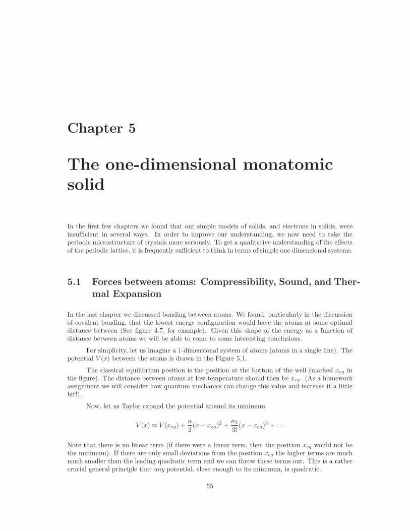
For simplicity, let us imagine a 1-dimensional system of atoms (atoms in a single line). Thepotential V (x) between the atoms is drawn in the Figure 5.1.

The classical equilibrium position is the position at the bottom of the well (marked xeq inthe figure). The distance between atoms at low temperature should then be xeq . (As a homeworkassignment we will consider how quantum mechanics can change this value and increase it a littlebit!).

Now, let us Taylor expand the potential around its minimum.

V (x) ≈ V (xeq) +κ

2(x− xeq)

2 +κ3

3!(x− xeq)

3 + . . .

Note that there is no linear term (if there were a linear term, then the position xeq would not bethe minimum). If there are only small deviations from the position xeq the higher terms are muchmuch smaller than the leading quadratic term and we can throw these terms out. This is a rathercrucial general principle that any potential, close enough to its minimum, is quadratic.

55

56 CHAPTER 5. THE ONE-DIMENSIONAL MONATOMIC SOLID

6

?

xmin

?

xmax

-?6kbT

V (x)

xxeq

Figure 5.1: Potential Between Neighboring Atoms (black). The red curve is a quadratic approx-imation to the minimum (it may look crooked but in fact the red curve is symmetric and theblack curve is asymmetric). The equilibrium position is xeq . At finite temperature T , the systemcan oscillate between xmax and xmin which are not symmetric around the minimum. Thus as Tincreases the average position moves out to larger distance and the system expands.

Compressibility (or Elasticity)

We thus have a simple Hooke’s law quadratic potential around the minimum. If we apply a forceto compress the system (i.e., apply a pressure to our model one dimensional solid) we find

−κ(δxeq) = F

where the sign is so that a positive (compressive) pressure reduces the distance between atoms.This is obviously just a description of the compressibility (or elasticity) of a solid. The usualdescription of compressibility is

β = −1

V

∂V

∂P

(one should ideally specify if this is measured at fixed T or at fixed S. Here, we are working atT = S = 0 for simplicity). In the 1d case, we write the compressibility as

β = −1

L

∂L

∂F=

1

κxeq=

1

κ a(5.1)

with L the length of the system and xeq is the spacing between atoms. Here we make the conven-tional definition that the equilibrium distance between identical atoms in a system (the so-calledlattice constant) is written as a.

Sound

You may recall from your fluids course that in an isotropic compressible fluid, one predicts soundwaves with velocity

v =

√

B

ρ=

√

1

ρβ(5.2)

5.2. MICOSCOPIC MODEL OF VIBRATIONS IN 1D 57

Here ρ is the mass density of the fluid, B is the bulk modulus, which is B = 1/β with β the(adiabatic) compressibility.

While in a real solid the compressibility is anisotropic and the speed of sound depends indetail on the direction of propagation, in our model 1d solid this is not a problem and we cancalculate that the the density is m/a with m the mass of each particle and a the equilibriumspacing between particles.

Thus using our result from above, we predict a sound wave with velocity

v =

√

κa2

m(5.3)

Shortly (in section 5.2.2) we will re-derive this expression from a microscopic equations of motionfor the atoms in the 1d solid.

Thermal Expansion

So far we have been working at zero temperature, but it is worth thinking at least a little bit aboutthermal expansion. This will be fleshed out more completely in a homework assignment. (In facteven in the homework assignment the treatment of thermal expansion will be very crude, but thatshould still be enough to give us the general idea of the phenomenon1).

Let us consider again figure 5.1 but now at finite temperature. We can imagine the potentialas a function of distance between atoms as being like a ball rolling around in a potential. At zeroenergy, the ball sits at the the minimum of the distribution. But if we give the ball some finitetemperature (i.e, some energy) it will oscillate around the minimum. At fixed energy kbT theball rolls back and forth between the points xmin and xmax where V (xmin) = V (xmax) = kbT .But away from the minimum the potential is asymmetric, so |xmax − xeq| > |xmin − xeq| so onaverage the particle has a position 〈x〉 > xeq(T = 0). This is in essence the reason for thermalexpansion! We will obtain positive thermal expansion for any system where κ3 < 0 (i.e., at smallx the potential is steeper) which almost always is true for real solids.

Summary

• Forces between atoms determine ground state structure.

• These same forces, perturbing around the ground state, determine elasticity, sound velocity,and thermal expansion.

• Thermal expansion comes from the non-quadratic part of the interatomic potential.

5.2 Micoscopic Model of Vibrations in 1d

In chapter 2 we considered the Boltzmann, Einstein, and Debye models of vibrations in solids.In this section we will consider a detailed model of vibration in a solid, first classically, andthen quantum mechanically. We will be able to better understand what these early attempts tounderstand vibrations achieved and we will be able to better understand their shortcomings.

1Although this description is an annoyingly crude discussion of thermal expansion, we are mandated by the IOPto teach something on this subject. Explaining it more correctly, is unfortunately, rather messy!


Let us consider a chain of identical atoms of mass m where the equilibrium spacing betweenatoms is a. Let us define the position of the nth atom to be xn and the equilibrium position of thenth atom to be xeq

n = na.

Once we allow motion of the atoms, we will have xn deviating from its equilibrium position,so we define the small variable

δxn = xn − xeqn

Note that in our simple model we are allowing motion of the masses only in one dimension (i.e.,we are allowing longitudinal motion of the chain, not transverse motion).

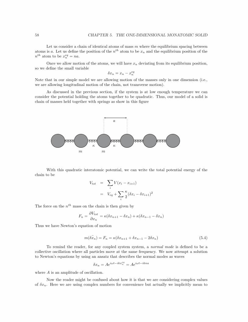
As discussed in the previous section, if the system is at low enough temperature we canconsider the potential holding the atoms together to be quadratic. Thus, our model of a solid ischain of masses held together with springs as show in this figure

a

m m

κ κ

With this quadratic interatomic potential, we can write the total potential energy of thechain to be

Vtot =∑

i

V (xi − xi+1)

= Veq +∑

i

κ

2(δxi − δxi+1)

2

The force on the nth mass on the chain is then given by

Fn =∂Vtot

∂xn= κ(δxn+1 − δxn) + κ(δxn−1 − δxn)

Thus we have Newton’s equation of motion

m( ¨δxn) = Fn = κ(δxn+1 + δxn−1 − 2δxn) (5.4)

To remind the reader, for any coupled system system, a normal mode is defined to be acollective oscillation where all particles move at the same frequency. We now attempt a solutionto Newton’s equations by using an ansatz that describes the normal modes as waves

δxn = Aeiωt−ikxeqn = Aeiωt−ikna

where A is an amplitude of oscillation.

Now the reader might be confused about how it is that we are considering complex valuesof δxn. Here we are using complex numbers for convenience but actually we implicitly mean to


take the real part. (This is analogous to what one does in circuit theory with oscillating currents!).Since we are taking the real part, it is sufficient to consider only ω > 0, however, we must becareful that k can then have either sign, and these are inequivalent once we have specified that ωis positive.

Plugging our ansatz into Eq. 5.4 we obtain

−mω2Aeiωt−ikna = κAeiωt[

e−ika(n+1) + e−ika(n−1) − 2e−ikan]

ormω2 = 2κ[1− cos(ka)] = 4κ sin2(ka/2) (5.5)

We thus obtain the result

ω = 2

√

κ

m

∣

∣

∣

∣

sin

(

ka

2

)∣

∣

∣

∣

(5.6)

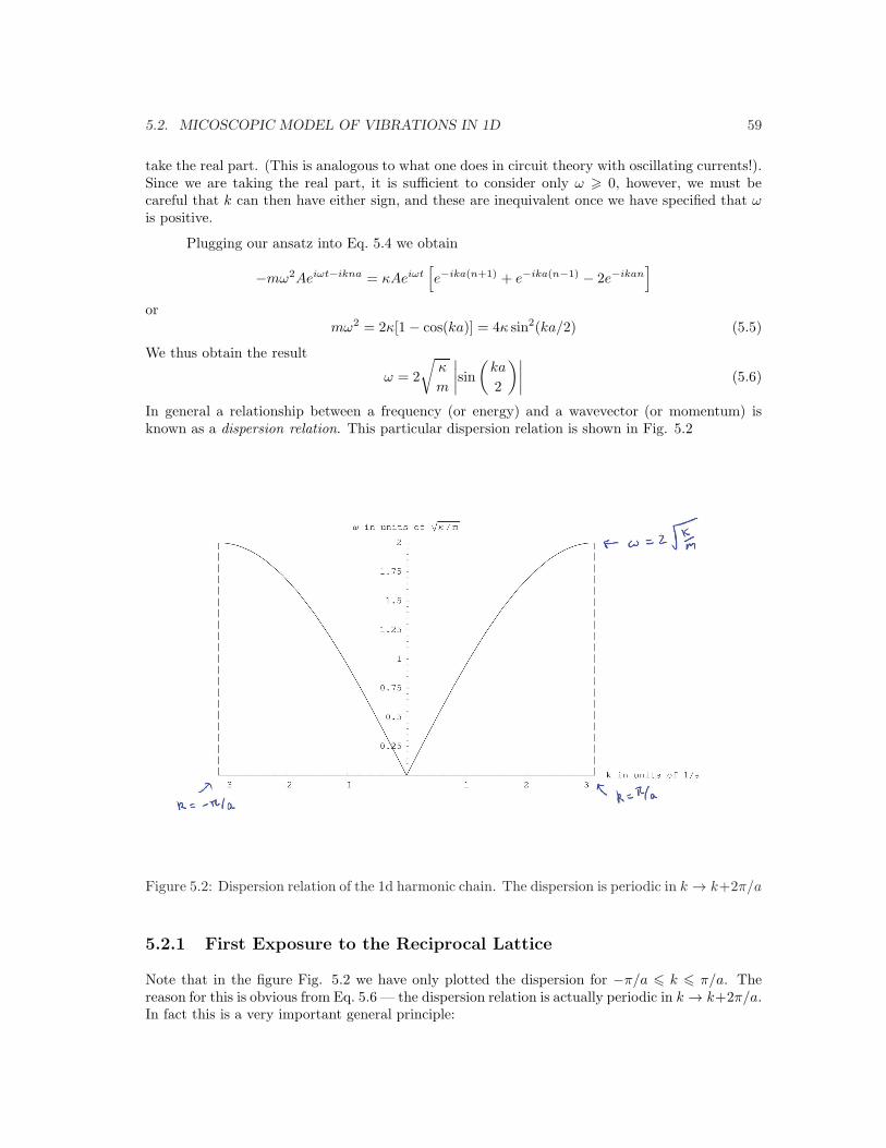
In general a relationship between a frequency (or energy) and a wavevector (or momentum) isknown as a dispersion relation. This particular dispersion relation is shown in Fig. 5.2 ! " # # " ! $%&'&%()*+#,-./"0./0./10##/"0#/0#/10"2%&'&%()*+3444444444445,6Figure 5.2: Dispersion relation of the 1d harmonic chain. The dispersion is periodic in k → k+2π/a

5.2.1 First Exposure to the Reciprocal Lattice

Note that in the figure Fig. 5.2 we have only plotted the dispersion for −π/a 6 k 6 π/a. Thereason for this is obvious from Eq. 5.6 — the dispersion relation is actually periodic in k → k+2π/a.In fact this is a very important general principle:


Principle 5.2.1: A system which is periodic in real space with aperiodicity a will be periodic in reciprocal space with periodicity 2π/a.

In this principle we have used the word reciprocal space which means k-space. In other words thisprinciple tells us that if a system looks the same when x→ x+a then in k-space the dispersion willlook the same when k → k + 2π/a. We will return to this principle many times in later chapters.

The periodic unit (the “unit cell”) in k-space is conventionally known as the Brillouin

Zone2,3. This is your first exposure to the concept of a Brillouin zone, but it again will play avery central role in later chapters. The “First Brillouin Zone” is a unit cell in k-space centeredaround the point k = 0. Thus in Fig. 5.2 we have shown only the first Brillouin zone, with theunderstanding that the dispersion is periodic for higher k. The points k = ±π/a are known as theBrillouin-Zone boundary and are defined in this case as being points which are symmetric aroundk = 0 and are separated by 2π/a.

It is worth pausing for a second and asking why we expect that the dispersion curve shouldbe periodic in k → k + 2π/a. Recall that we defined our vibration mode to be of the form

δxn = Aeiωt−ikna (5.7)

If we take k → k + 2π/a we obtain

δxn = Aeiωt−i(k+2π/a)na = Aeiωt−iknae−i2πn = Aeiωt−ikna

where here we have usede−i2πn = 1

for any integer n. What we have found here is that shifting k → k+2π/a gives us back exactly thesame oscillation mode the we had before we shifted k. The two are physically exactly equivalent!

In fact, it is similarly clear that shifting k by any k + 2πp/a with p an integer since, willgive us back exactly the same wave also since

e−i2πnp = 1

as well. We can thus define a set of points in k-space (reciprocal space) which are all physicallyequivalent to the point k = 0. This set of points is known as the reciprocal lattice. The originalperiodic set of points xn = na is known as the direct lattice or real-space lattice to distinguish itfrom the reciprocal lattice, when necessary.

The concept of the reciprocal lattice will extremely important later on. We can see theanalogy between the direct lattice and the reciprocal lattice as follows:

Direct lattice: xn = . . . − 2a, −a, 0, a, 2a, . . .

Reciprocal lattice: Gn = . . . − 2

(

2π

a

)

, −2π

a, 0,

2π

a, 2

(

2π

a

)

, . . .

Note that the defining property of the reciprocal lattice in terms of the points in the real latticecan be given as

eiGmxn = 1 (5.8)

A point Gm is a member of the reciprocal lattice iff Eq. 5.8 is true for all xn in the real lattice.

2Leon Brillouin was one of Sommerfeld’s students. He is famous for many things including for being the “B” inthe “WKB” approximation. I’m not sure if WKB is on your syllabus, but it really should be if it is not already!

3The pronunciation of “Brillouin” is something that gives English speakers a great deal of difficulty. If you speakFrench you will probably cringe at the way this name is butchered. (I did badly in French in school, so I’m probablyone of the worst offenders.) According to online dictionaries it is properly pronounced somewhere between thefollowing words: brewan, bree-wah, breel-wahn, bree(y)wa(n), and bree-l-(uh)-wahn. At any rate, the “l” and the“n” should both be very weak.


5.2.2 Properties of the Dispersion of the 1d chain

We now return to more carefully examine the properties of the dispersion we calculated (Eq. 5.6).

Sound Waves:

Recall that sound wave4 is a vibration that has a long wavelength (compared to the inter-atomicspacing). In this long wavelength regime, we find the dispersion we just calculated to be linearwith wavevector ω = vsoundk as expected for sound with

vsound = a

√

κ

m.

(To see this, just expand the sin in Eq. 5.6). Note that this sound velocity matches the velocitypredicted from Eq. 5.3.

However, we note that at larger k, the dispersion is no longer linear. This is in disagreementwith what Debye assumed in his calculation in section 2.2. So clearly this is a shortcoming ofthe Debye theory. In reality the dispersion of normal modes of vibration is linear only at longwavelength.

At shorter wavelength (larger k) one typically defines two different velocities: The group

velocity, the speed at which a wavepacket moves, is given by

vgroup = dω/dk

And the phase velocity, the speed at which the individual maxima and minima move, is given by

vphase = ω/k

These two match in the case of a linear dispersion, but otherwise are different. Note that the groupvelocity becomes zero at the Brillouin zone boundaries k = ±π/a (i.e., the dispersion is flat). Aswe will see many times later on, this is a general principle!

Counting Normal Modes:

Let us now ask how many normal modes there are in our system. Naively it would appear thatwe can put any k such that −π/a 6 k < π/a into Eq. 5.6 and obtain a new normal mode withwavevector k and frequency ω(k). However this is not precisely correct.

Let us assume our system has exactly N masses in a row, and for simplicity let us assumethat our system has periodic boundary conditions i.e., particle x0 has particle x1 to its right andparticle xN−1 to its left. Another way to say this is to let, xn+N = xn, i.e., this one dimensionalsystem forms a big circle. In this case we must be careful that the wave ansatz Eq. 5.7 makessense as we go all the way around the circle. We must therefore have

eiωt−ikna = eiωt−ik(N+n)a

Or equivalently we must haveeikNa = 1

4For reference it is good to remember that humans can hear sound wavelengths roughly between 1cm and 10m.Both of these are very long wavelength compared to interatomic spacings.


This requirement restricts the possible values of k to be of the form

k =2πp

Na=

2πp

L

where p is an integer and L is the total length of the system. Thus k becomes quantized ratherthan a continuous variable. This means that the k-axis in Figure 5.2 is actually a discrete set ofmany many individual points; the spacing between two of these consecutive points being 2π/(Na).

Let us now count how many normal modes we have. As mentioned above in our discussionof the Brillouin zone, adding 2π/a to k brings one back to exactly the same physical wave. Thuswe only ever need consider k values within the first Brillouin zone (i.e., −π/a 6 k < pi/a (sinceπ/a is the same as −π/a we choose to count one but not the other). Thus the total number ofnormal modes is

Total Number of Modes =Range of k

Spacing between neigboring k=

2π/a

2π/(Na)= N (5.9)

There is precisely one normal mode per mass in the system — that is, one normal mode per degreeof freedom in the whole system. This is what Debye insightfully predicted in order to cut off hisdivergent integrals in section 2.2.3 above!

5.2.3 Quantum Modes: Phonons

We now make a rather important leap from classical to quantum physics.

Quantum Correspondence: If a classical harmonic system (i.e., anyquadratic hamiltonian) has a normal oscillation mode at frequency ωthe corresponding quantum system will have eigenstates with energy

En = ~ω(n+1

2) (5.10)

Presumably

you know this well in the case of a single harmonic oscillator. The only thing different here is thatthe harmonic oscillator is a collective normal mode not just motion of a single particle. Thisquantum correspondence principle will be the subject of a homework assignment.

Thus at a given wavevector k, there are many possible eigenstates, the ground state beingthe n = 0 eigenstate which has only the zero-point energy ~ω(k)/2. The lowest energy excitationis of energy ~ω(k) greater than the ground state corresponding to the excited n = 1 eigenstate.Generally all excitations at this wavevector occur in energy units of ~ω(k), and the higher valuesof energy correspond classically to oscillations of increasing amplitude.

Each excitation of this “normal mode” by step up the harmonic oscillator excitation ladder(increasing the quantum number n) is known as a “phonon”.

Definition 5.2.1. A phonon is a discrete quanta of vibration5

This is entirely analogous to defining a single quanta of light as a photon. As is the casewith the photon, we may think of the phonon as actually being a particle, or we can think of thephonon as being a quantized wave.

5I do not like the definition of a phonon as “a quanta of vibrational energy” which many books use. The vibrationdoes carry indeed energy, but it carries other quantum numbers (such as crystal momentum) as well, so why specifyenergy only?


If we think about the phonon as being a particle (as with the photon) then we see that wecan put many phonons in the same state (ie., the quantum number n in Eq. 5.10 can be increasedto any value), thus we conclude that phonons, like photons, are bosons. As with photons, at finitetemperature there will be a nonzero number of phonons (i.e., n will be on average nonzero) asgiven by the Bose occupation factor.

nB(βω) =1

eβω − 1

with β = 1/(kbT ) and ω the oscillation frequency.

Thus, the expectation of the phonons at wavevector k is given by

Ek = ~ω(k)

(

nB(βω(k)) +1

2

)

We can use this type of expression to calculate the heat capacity of our 1d model6

Utotal =∑

k

~ω(k)

(

nB(βω(k)) +1

2

)

where the sum over k here is over all possible normal modes, i.e, k = 2πp/(Na) such that −π/a 6

k < π/a. Thus we really mean

∑

k

→

N/2−1∑

p=−N/2

|k=(2πp)/(Na)

Since for a large system, the k points are very close together, we can convert the discrete sum intoan integral (something we should be very familiar with by now) to obtain

∑

k

→Na

2π

∫ π/a

−π/a

dk

Note that we can use this continuum integral to count the total number of modes in the system

Na

2π

∫ π/a

−π/a

dk = N

as predicted by Debye.

Using this integral form of the sum we have the total energy given by

Utotal =N

2π

∫ π/a

−π/a

dk ~ω(k)

(

nB(βω(k)) +1

2

)

from this we could calculate specific heat as dU/dT .

These two previous expressions look exactly like what Debye would have obtained from hiscalculation (for a 1d version of his model)! The only difference lies in our expression for ω(k).Debye only knew about sound where ω = vk, is linear in wavevector. We, on the other hand, have

6The observant reader will note that we are calculating CV = dU/dT the heat capacity at constant volume.Why constant volume? As we saw above when we studied thermal expansion, the crystal does not expand unlesswe include third order (or higher) order terms in the interatomic potential, which are not in this model!


just calculated that for our microscopic ball and spring model ω is not linear in k. In fact, Einstein’scalculation of specific heat can be phrased in exactly the same language. Only for Einstein’s modelω = ω0 is constant for all k. We thus see Einstein’s model, Debye’s model, and our microscopicharmonic model in a very unified light. The only difference between the three is what we use fora dispersion relation.

One final comment is that it is frequently useful to further replace integrals over k withintegrals over frequency (we did this when we studied the Debye model above). We obtain generally

Na

2π

∫ π/a

−π/a

dk =

∫

dωg(ω)

where7

g(ω) = 2Na

2π|dk/dω|

Note that in the (1d) Debye model this density of states is constant from ω = 0 to ω = ωDebye =vπ/a. In our model, as we have calculated above, the density of states is not a constant, butbecomes zero at frequency above the maximum frequency 2

√

κ/m. (In a homework problem wecalculate this density of states explicitly). Finally in the Einstein model, this density of states is adelta-function at frequency ω0.

5.2.4 Comments on Reciprocal Space II: Crystal Momentum

As mentioned above, the wavevector of a phonon is defined only modulo the reciprocal lattice. Inother words, k is the same as k + Gm where Gm = 2πm/a is a point in the reciprocal lattice.Now we are supposed to think of these phonons as particles – and we like to think of our particlesas having energy ~ω and a momentum ~k. But we cannot define a phonon’s momentum thisway because physically it is the same phonon whether we describe it as ~k or ~(k + Gm). Wethus instead define a concept known as the crystal momentum which is the momentum modulothe reciprocal lattice — or equivalently we agree that we must always describe k within the firstBrillouin zone.

In fact, this idea of crystal momentum is extremely powerful. Since we are thinking aboutphonons as being particles, it is actually possible for two (or more) phonons to bump into eachother and scatter from each other — the same way particles do8. In such a collision, energyis conserved and crystal momentum is conserved! For example three phonons each with crystalmomentum ~(2/3)π/a can scatter off of each other to produce three phonons each with crystalmomentum −~(2/3)π/a. This is allowed since the initial and final states have the same energyand

3× (2/3)π/a = 3× (−2/3)π/a mod (2π/a)

During these collisions although momentum ~k is not conserved, crystal momentum is9. In fact,the situation is similar when, for example, phonons scatter from electrons in a periodic lattice –

7The factor of 2 out front comes from the fact that each ω occurs for the two possible values of ±k.8In the harmonic model we have considered phonons do not scatter from each other. We know this because

the phonons are eigenstates of the system, so their occupation does not change with time. However, if we addanharmonic (cubic and higher) terms to the inter-atomic potential, this corresponds to perturbing the phononhamiltonian and can be interpreted as allowing phonons to scatter from each other.

9This thing we have defined ~k has dimensions of momentum, but is not conserved. However, as we will discussbelow in chapter 10, if a particle, like a photon, enters a crystal with a given momentum and undergoes a processthat conserves crystal momentum but not momentum, when the photon exits the crystal we will find that totalmomentum of the system is indeed conserved, with the momentum of the entire crystal accounting for any momentumthat is missing from the photon. See footnote 5 in section 10.1.1

5.3. SUMMARY OF THE ONE-DIMENSIONAL CHAIN 65

crystal momentum becomes the conserved quantity rather than momentum. This is an extremelyimportant principle which we will encounter again and again. In fact, it is a main cornerstone ofsolid-state physics.

Aside: There is a very fundamental reason for the conservation of crystal momentum. Conserved

quantities are results of symmetries (this is a deep and general statement known as Noether’s theorem10). For

example, conservation of momentum is a result of the translational invariance of space. If space is not the

same from point to point, for example if there is a potential V (x) which is different at different places, then

momentum is not conserved. The conservation of crystal momentum correspondingly results from space being

invariant under translations of a, giving us momentum that is conserved modulo 2π/a.

5.3 Summary of the one-dimensional chain

A number of very crucial new ideas have been introduced in this section. Many of these will returnagain and again in later chapters.

• Normal modes are collective oscillations where all particles move at the same frequency.

• If a system is periodic in space with periodicity ∆x = a, then in reciprocal space (k-space)the system is periodic with periodicity ∆k = 2π/a.

• Values of k which differ by multiples of 2π/a are physically equivalent. The set of points ink-space which are equivalent to k = 0 are known as the reciprocal lattice.

• Any values of k is equivalent to some k in the first Brillouin-zone, −π/a 6 k < π/a (in 1d).

• The sound velocity is the slope of the dispersion in the small k limit (group = phase velocityin this limit).

• A classical normal mode of frequency ω gets translated into quantum mechanical eigenstatesEn = ~ω(n + 1

2 ). If the system is in the nth eigenstate, we say that it is occupied by nphonons.

• Phonons can be thought of as particles, like photons, that obey Bose statistics.

References

Sound and compressibility:

• Goodstein, section 3.2b.

• Ibach an Luth, beginning of section 4.5

• Hook and Hall, section 2.2

Thermal Expansion (Most references go into way too much depth on thermal expansion):

• Kittel chapter 5, section on thermal expansion.

10Emmy Noether has been described by Einstein, among others, as the most important woman in the history ofmathematics.


Normal Modes of Monatomic Chain and introduction to phonons:

• Kittel, beginning of chapter 4

• Goodstein, beginning of section 3.3

• Hook and Hall, section 2.3.1

• Burns, section 12.1-12.2

• Ashcroft and Mermin, beginning of chapter 22.

Chapter 6

The one-dimensional diatomic

solid

In the previous chapter we studied in detail a one dimensional model of a solid where every atom isidentical to every other atom. However, in real materials not every atom is the same (for example,in Sodium Chloride, we have two types of atoms!). We thus intend to generalize our previousdiscussion of the one dimension solid to a one dimensional solid with two types of atoms. Much ofthis will follow the outline set in the previous chapter, but we will see that several fundamentallynew features will now emerge.

6.1 Diatomic Crystal Structure: Some useful definitions

Consider the following model system

m1 m2

κ1 κ2

m1 m2

κ1 κ2

Fig. 6.1.1

Which represents a periodic arrangement of two different types of atoms. Here we havegiven them two masses m1 and m2 and the springs which alternate along the 1-dimensional chain.The springs connecting the atoms have spring constants κ1 and κ2 and also alternate.

In this circumstance with more than one type of atom, we first would like to identify theso-called unit cell which is the repeated motif in the arrangement of atoms. In this picture, we haveput a box around the unit cell. The length of the unit cell in 1d is known as the lattice constant

67

68 CHAPTER 6. THE ONE-DIMENSIONAL DIATOMIC SOLID

and it is labeled a.

a

Fig. 6.1.2

Note however, that the definition of the unit cell is extremely non-unique. We could just aswell have chosen (for example) the unit cell to be as follows.

Fig. 6.1.3

a

The important thing in defining a periodic system is to choose some unit cell and thenconstruct the full system by reproducing the same unit cell over and over. (In other words, makea definition of the unit cell and stick with that definition!).

It is sometimes useful to pick some references point inside each unit cell. This set of referencepoints makes a simple lattice (we will define the term “lattice” more closely in later chapters –but for now the point is that a lattice has only one type of point in it – not two different types ofpoints). So in this figure, we have marked our reference point in each unit cell with an X (again,the choice of this reference point is arbitrary).

6.2. NORMAL MODES OF THE DIATOMIC SOLID 69

a

XX X Fig. 6.1.4

7a20

3a40

r1 r2 r3

Given the reference lattice point in the unit cell, the description of all of the atoms in theunit cell with respect to this reference point is known as a basis. In this case we might describeour basis as

light gray atom centered at position 3a/40 to left of reference lattice point

dark gray atom centered at position 7a/20 to right of reference lattice point

Thus if the reference lattice point in unit cell n is called rn (and the spacing between the latticepoints is a) we can set

rn = an

with a the size of the unit cell. Then the (equilibrium) position of the light gray atom in the nth

unit cell isxeqn = an− 3a/40

whereas the (equilibrium) position of the dark gray atom in the nth unit cell is

yeqn = an+ 7a/20

6.2 Normal Modes of the Diatomic Solid

For simplicity, let us focus on the case where all of the masses along our chain are the samem1 = m2 = m but the two spring constants κ1 and κ2 are different. (For homework we willconsider the case where the masses are different, but the spring constants are the same!).

Fig. 6.2.1

x1 y1 x2

κ1 κ2

y2 x3 y3

κ1 κ2

m m m m m m


Given the spring constants in the picture, we can write down Newton’s equations of of motionfor the deviations of the positions of the masses from their equilibrium positions. We obtain

m δxn = κ2(δyn − δxn) + κ1(δyn−1 − δxn) (6.1)

m δyn = κ1(δxn+1 − δyn) + κ2(δxn − δyn) (6.2)

Analogous to the one dimensional case we propose ansatze1 for these quantities that have the formof a wave

δxn = Axeiωt−ikna (6.3)

δyn = Ayeiωt−ikna (6.4)

where, as in the previous chapter, we implicitly mean to take the real part of the complex number.As such, we can always choose to take ω > 0 as long as we consider k to be either positive andnegative

As we saw in the previous chapter, values of k that differ by 2π/a are physically equivalent.We can thus focus our attention to the first Brillouin zone −π/a 6 k < π/a. Note that theimportant length here is the unit cell length or lattice constant a. Any k outside the first Brillouinzone is redundant with some other k inside the zone.

As we found in the previous chapter, if our system has N unit cells, then (putting periodicboundary conditions on the system) k will be is quantized in units of 2π/(Na) = 2π/L. Note thathere the important quantity is N , the number of unit cells, not the number of atoms (2N).

Dividing the range of k in the first Brillouin zone by the spacing between neighboring k’s,we obtain exactly N different possible values of k exactly as we did in Eq. 5.9. In other words, wehave exactly one value of k per unit cell.

We might recall at this point the intuition that Debye used — that there should be exactlyone possible excitation mode per degree of freedom of the system. Here we obviously have twodegrees of freedom per unit cell, but we obtain only one possible value of k per unit cell. Theresolution, as we will see in a moment, is that there will be two possible oscillation modes for eachwavevector k.

We now proceed by plugging in our ansatze (Eq. 6.3 and 6.4) into our equations of motion(Eq. 6.1 and 6.2). We obtain

−ω2mAxeiωt−ikna = κ2Aye

iωt−ikna + κ1Ayeiωt−ik(n−1)a − (κ1 + κ2)Axe

iωt−ikna

−ω2mAyeiωt−ikna = κ1Axe

iωt−ik(n+1)a + κ2Axeiωt−ikna − (κ1 + κ2)Aye

iωt−ikna

which simplifies to

−ω2mAx = κ2Ay + κ1Ayeika − (κ1 + κ2)Ax

−ω2mAy = κ1Axe−ika + κ2Ax − (κ1 + κ2)Ay

This can be rewritten conveniently as an eigenvalue equation

mω2

(

Ax

Ay

)

=

(

(κ1 + κ2) −κ2 − κ1eika

−κ2 − κ1e−ika (κ1 + κ2)

)(

Ax

Ay

)

(6.5)

The solutions of this are obtained by finding the zeros of the secular determinant

0 =

∣

∣

∣

∣

(κ1 + κ2)−mω2 −κ2 − κ1eika

−κ2 − κ1e−ika (κ1 + κ2)−mω2

∣

∣

∣

∣

=∣

∣(κ1 + κ2)−mω2∣

∣

2− |κ2 + κ1e

ika|2

1I believe this is the proper pluralization of ansatz.


The roots of which are clearly given by

mω2 = (κ1 + κ2)± |κ1 + κ2eika|

The second term needs to be simplified

|κ1 + κ2eika| =

√

(κ1 + κ2eika)(κ1 + κ2e−ika) =√

κ21 + κ2

2 + 2κ1κ2 cos(ka)

So we finally obtain

ω± =

√

κ1 + κ2

m±

1

m

√

κ21 + κ2

2 + 2κ1κ2 cos(ka) (6.6)

Note in particular that for each k we find two normal modes — thus since there are N differentk values, we obtain 2N modes total (if there are N unit cells in the entire system). This is inagreement with our above discussion that we should have exactly one normal mode per degree offreedom in our system.

The dispersion of these two modes is shown in Figure 6.1. ! " # # " ! $%&'#&'"&'!&'())'#*+,-,+./01233333333333333333333333333333333#456)76#89:Figure 6.1: Dispersion relation of the 1d diatomic chain. The dispersion is periodic in k → k+2π/a.Here the dispersion is shown for the case of κ2 = 1.4κ1. This scheme of plotting dispersions,putting all normal modes within the first Brillouin zone, is the reduced zone scheme. Compare thisto Fig. 6.2 below.

A few things to note about this dispersion. First of all we note that there is a long wavelengthlow energy mode with linear dispersion (corresponding to ω− in Eq. 6.6). This is the sound wave, oracoustic mode. Generally the definition of an acoustic mode is any mode that has linear dispersionas k → 0. These correspond to sound waves.


By expanding Eq. 6.6 for small k it is easy to check that the sound velocity is

vsound =dω−dk

=

√

a2κ1κ2

2m(κ1 + κ2)(6.7)

In fact, we could have calculated this sound velocity on general principles analogous to what wedid in Eq. 5.2. The density of the chain is 2m/a. The effective spring constant of two springs κ1

and κ2 in series is κ = (κ1 + κ2)/(κ1κ2) so the compressibility of the chain is β = 1/(κa) (See Eq.5.1). Then plugging into Eq. 5.2 gives exactly the same sound velocity as we calculate here in Eq.6.7.

The higher energy branch of excitations is known as the optical mode. It is easy to checkthat in this case the optical mode goes to frequency

√

2(κ1 + κ2)/m at k = 0, and also has zerogroup velocity at k = 0. The reason for the nomenclature “optical” will become clearer later in thecourse when we study scattering of light from solids. However, here is a very simplified descriptionof why it is named this way: Consider a solid being exposed to light. It is possible for the lightto be absorbed by the solid, but energy and momentum must both be conserved. However, lighttravels at a very high velocity c, so ω = ck is a very large number. Since phonons have a maximumfrequency, this means that photons can only be absorbed for very small k. However, for small k,acoustic phonons have energy vk � ck so that energy and momentum cannot be conserved. Onthe other hand, optical phonons have energy ωoptical which is finite for small k so that at somevalue of small k, we have ωoptical = ck and one can match the energy and momentum of the photonto that of the phonon.2 Thus, whenever phonons interact with light, it is inevitably the opticalphonons that are involved.

Let us examine a bit more closely the acoustic and the optical mode as k → 0. Examiningour eigenvalue problem Eq. 6.5, we see that in this limit the matrix to be diagonalized takes thesimple form

ω2

(

Ax

Ay

)

=κ1 + κ2

m

(

1 −1−1 1

)(

Ax

Ay

)

(6.8)

The acoustic mode (which has frequency 0) is solved by the eigenvector

(

Ax

Ay

)

=

(

11

)

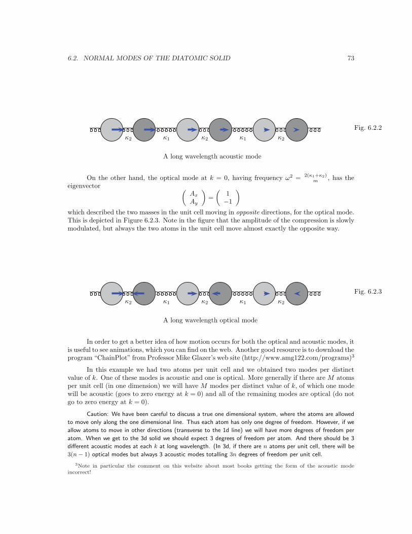
This tells us that the two masses in the unit cell (at positions x and y) move together for thecase of the acoustic mode in the long wavelength limit. This is not surprising considering ourunderstanding of sound waves as being very long wavelength compressions and rarifactions. Thisis depicted in Figure 6.2.2. Note in the figure that the amplitude of the compression is slowlymodulated, but always the two atoms in the unit cell move almost exactly the same way.

2From this naive argument, one might think that the process where one photon with frequency ωoptical isabsorbed while emitting a phonon is an allowed process. This is not true since the photons carry spin and spinmust also be conserved. Much more typically the interaction between photons and phonons is one where a photonis absorbed and then re-emitted. I.e., it is inelastically scattered. We will discuss this later on.


Fig. 6.2.2

κ2 κ1 κ2 κ1 κ2

A long wavelength acoustic mode

On the other hand, the optical mode at k = 0, having frequency ω2 = 2(κ1+κ2)m , has the

eigenvector(

Ax

Ay

)

=

(

1−1

)

which described the two masses in the unit cell moving in opposite directions, for the optical mode.This is depicted in Figure 6.2.3. Note in the figure that the amplitude of the compression is slowlymodulated, but always the two atoms in the unit cell move almost exactly the opposite way.

Fig. 6.2.3

κ2 κ1 κ2 κ1 κ2

A long wavelength optical mode

In order to get a better idea of how motion occurs for both the optical and acoustic modes, itis useful to see animations, which you can find on the web. Another good resource is to download theprogram “ChainPlot” from Professor Mike Glazer’s web site (http://www.amg122.com/programs)3

In this example we had two atoms per unit cell and we obtained two modes per distinctvalue of k. One of these modes is acoustic and one is optical. More generally if there are M atomsper unit cell (in one dimension) we will have M modes per distinct value of k, of which one modewill be acoustic (goes to zero energy at k = 0) and all of the remaining modes are optical (do notgo to zero energy at k = 0).

Caution: We have been careful to discuss a true one dimensional system, where the atoms are allowed

to move only along the one dimensional line. Thus each atom has only one degree of freedom. However, if we

allow atoms to move in other directions (transverse to the 1d line) we will have more degrees of freedom per

atom. When we get to the 3d solid we should expect 3 degrees of freedom per atom. And there should be 3

different acoustic modes at each k at long wavelength. (In 3d, if there are n atoms per unit cell, there will be

3(n− 1) optical modes but always 3 acoustic modes totalling 3n degrees of freedom per unit cell.

3Note in particular the comment on this website about most books getting the form of the acoustic modeincorrect!


One thing that we should study closely is the behavior at the Brillouin zone boundary. Itis also easy to check that the frequencies ω± at the zone boundary (k = ±π/a) are

√

κ1/m and√

κ2/m, the larger of the two being ω+. We can also check that the group velocity dω/dk of bothmodes goes to zero at the zone boundary (Similarly the optical mode has zero group velocity atk = 0).

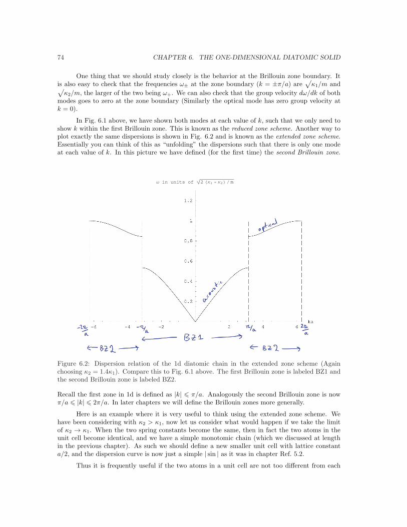
In Fig. 6.1 above, we have shown both modes at each value of k, such that we only need toshow k within the first Brillouin zone. This is known as the reduced zone scheme. Another way toplot exactly the same dispersions is shown in Fig. 6.2 and is known as the extended zone scheme.Essentially you can think of this as “unfolding” the dispersions such that there is only one modeat each value of k. In this picture we have defined (for the first time) the second Brillouin zone. ! " # # " ! $%&'#&'"&'!&'())'#*+,-,+./01233333333333333333333333333333333#456)76#89:Figure 6.2: Dispersion relation of the 1d diatomic chain in the extended zone scheme (Againchoosing κ2 = 1.4κ1). Compare this to Fig. 6.1 above. The first Brillouin zone is labeled BZ1 andthe second Brillouin zone is labeled BZ2.

Recall the first zone in 1d is defined as |k| 6 π/a. Analogously the second Brillouin zone is nowπ/a 6 |k| 6 2π/a. In later chapters we will define the Brillouin zones more generally.

Here is an example where it is very useful to think using the extended zone scheme. Wehave been considering with κ2 > κ1, now let us consider what would happen if we take the limitof κ2 → κ1. When the two spring constants become the same, then in fact the two atoms in theunit cell become identical, and we have a simple monotomic chain (which we discussed at lengthin the previous chapter). As such we should define a new smaller unit cell with lattice constanta/2, and the dispersion curve is now just a simple | sin | as it was in chapter Ref. 5.2.

Thus it is frequently useful if the two atoms in a unit cell are not too different from each

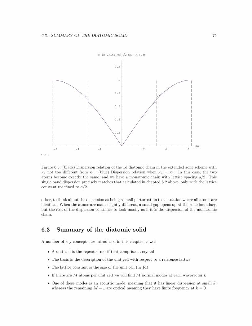
6.3. SUMMARY OF THE DIATOMIC SOLID 75 ! " # # " ! $%&'#&'"&'!&'())'#*+,-,+./01233333333333333333333333333333333#456)76#89:;<=>?@ABCFigure 6.3: (black) Dispersion relation of the 1d diatomic chain in the extended zone scheme withκ2 not too different from κ1. (blue) Dispersion relation when κ2 = κ1. In this case, the twoatoms become exactly the same, and we have a monatomic chain with lattice spacing a/2. Thissingle band dispersion precisely matches that calculated in chapted 5.2 above, only with the latticeconstant redefined to a/2.

other, to think about the dispersion as being a small perturbation to a situation where all atoms areidentical. When the atoms are made slightly different, a small gap opens up at the zone boundary,but the rest of the dispersion continues to look mostly as if it is the dispersion of the monatomicchain.

6.3 Summary of the diatomic solid

A number of key concepts are introduced in this chapter as well

• A unit cell is the repeated motif that comprises a crystal

• The basis is the description of the unit cell with respect to a reference lattice

• The lattice constant is the size of the unit cell (in 1d)

• If there are M atoms per unit cell we will find M normal modes at each wavevector k

• One of these modes is an acoustic mode, meaning that it has linear dispersion at small k,whereas the remaining M − 1 are optical meaning they have finite frequency at k = 0.


• For the acoustic mode, all atoms in the unit cell move in-phase with each other, whereas foroptical modes, they move out of phase with each other

• Except for the acoustic mode, all other excitation branches have zero group velocity fork = nπ/a for any n.

• If all of the dispersion curves are plotted within the first Brillouin zone |k| 6 π/a we call thisthe reduced zone scheme. If we “unfold” the curves such that there is only one excitationplotted per k, but we use more than one Brillouin zone, we call this the extended zone scheme.

• If the two atoms in the unit cell become identical, the new unit cell is half the size of the oldunit cell. It is convenient to describe this limit in the extended zone scheme.

References

• Ashcroft and Mermin, chapter 22 (but not the 3d part)

• Ibach and Luth, section 4.3

• Kittel, chapter 4

• Hook and Hall, sections 2.3.2, 2.4, 2.5

• Burns, section 12.3

Documents

The one-dimensional monatomic solid - WordPress.com · The one-dimensional monatomic solid In the ﬁrst few chapters we found that our simple models of solids, and electrons in solids,