Generated using version 3.0 of the official AMS LATEX template

The Ocean Circulation in Thermohaline1

Coordinates2

Jan D. Zika,∗3

Matthew H. England and Willem P. Sijp

The Climate Change Research Centre, The University of New South Wales, Australia

4

For the Journal of Physical Oceanography5

August 3, 20116

∗Corresponding author address: The Climate Change Research Centre, University of New South Wales,

2037, NSW, Australia.

E-mail: J.Zika@unsw.edu.au

1

ABSTRACT7

The thermohaline streamfunction is presented. The thermohaline streamfunction is the in-8

tegral of transport in temperature - salinity space and represents the net pathway of oceanic9

water parcels in that space. The thermohaline streamfunction is proposed as a diagnostic to10

understand the global oceanic circulation and its role in the global movement of heat and11

freshwater. The coordinate system used is fully Lagrangian. As such, physical pathways12

and ventilation timescales are naturally diagnosed, as are the roles of the mean flow and13

turbulent fluctuations. As potential density is a function of temperature and salinity, the14

framework is naturally isopycnal and is ideal for the diagnosis of water-mass transformations15

and advective diapycnal heat and freshwater transports. Crucially, the thermohaline stream-16

function is computationally and practically trivial to implement as a diagnostic for ocean17

models. Here, the thermohaline streamfunction is computed using the output of an equili-18

brated intermediate complexity climate model. It describes a global cell, a warm tropical19

cell and a bottom water cell. The streamfunction computed from eddy-induced advection is20

equivalent in magnitude to that from the total advection, demonstrating the zero order im-21

portance of parameterised eddy fluxes in oceanic heat and freshwater transports. The global22

cell, being clockwise in thermohaline space, tends to advect both heat and salt towards23

denser (poleward) water-masses in symmetry with the atmosphere’s poleward transport of24

moisture. A re-projection of the global cell, from thermohaline to geographical coordinates25

reveals a thermohaline mean circulation reminiscent of the schematised ‘global conveyor’.26

1

1. Introduction27

It has long been recognised that the ocean displays variability across a large spectrum of28

spatial scales, from global scale oceanic gyres and circumpolar currents to millimetre scale29

turbulent motions, and on a myriad of temporal scales from millennial overturning to waves30

with micro second periods (Davis et al. 1981). All temporal and spatial scales of motion31

contribute to the global ocean circulation and its role in the climate system (Munk and32

Wunsch 1998). Despite this, descriptive oceanographers have identified specific pathways of33

net oceanic motion from observed tracers fields (Wust 1935; Deacon 1937; Gordon 1986).34

These pathways have been schematised in a variety of ways, the ‘global conveyor’ of Broecker35

(1991) being the most universally recognised (see Richardson 2008, for a review of such36

schematics).37

Over the past half century, numerical models have moved to finer and finer resolution38

and have progressively resolved an increasing number of scales. A key challenge remains39

however: distilling the plethora of motions of a numerical model into simplified indices and40

diagrams with minimal loss of information. It is pertinent, also, to test integral metrics of41

the ocean circulation and quantify how they relate to the climate system.42

A common way of understanding the global circulation is to average oceanic velocities43

at constant latitude and depth and look at the circulation in a meridional-vertical coordi-44

nate. The circulation revealed is known as the Meridional Overturning Circulation (MOC,45

Kuhlbrodt et al. 2007). The MOC describes net vertical and meridional motion. it is often46

used to infer how the ocean distributes properties around the globe by transposing the diag-47

nosed MOC onto zonally averaged quantities. This approach is somewhat valid in the North48

2

Atlantic where a strong mean overturning exists and properties are reasonably homogeneous49

at constant depth and latitude. In other regions however, overturning cells in the depth-50

latitude plane do not correspond to property transports at all. In the Southern Ocean, for51

example, a vigorous ‘Deacon Cell’ exists, apparently driving 30-40 Sv of light surface water52

down to the depth of Drake Passage at around 2000m (Manabe et al. 1990). However, when53

the circulation is averaged in density-latitude space, correlations between the meridional54

velocity and the thickness of density layers counter the Deacon Cell (Doos and Webb 1994).55

Thus, by averaging the flow in density, rather than depth space, a complimentary view, more56

consistent with the distribution of tracers, is revealed.57

In the example of the Southern Ocean, the vertical coordinate, density, is used to capture58

meridional exchanges of water-masses. Nycander et al. (2007) and Nurser and Lee (2004)59

propose diagnosing the ocean circulation in density - depth coordinates to capture the vertical60

exchanges of water-masses. Using this approach, Zika (2011) demonstrate that the processes61

which contribute to meridional exchanges of water-masses in the Southern Ocean can be62

very different to those which contribute to vertical exchanges. Boccaletti et al. (2005) and63

Ferrari and Ferreira (2011) have analysed the meridional circulation in temperature-latitude64

coordinates and reveal a different circulation to that in density-latitude coordinates. O65

Observed tracer distributions reveal oceanic exchanges of both heat and salt which are66

not only meridional, but also zonal, between ocean basins, and vertical, between the ocean67

surface and the interior (e.g. Broecker 1991; Gordon 1991; Schmitz 1996). We seek a68

coordinate system which captures this net global circulation.69

Principally, the MOC is considered important in the climate system because of its role70

in transporting heat, freshwater, nutrients and carbon. By transporting heat and freshwater71

3

around the globe the ocean influences global temperatures and plays a key role in the hydro-72

logical cycle. The water-masses through which the global-conveyor is thought to travel are73

each defined by unique temperature and salinity properties. Here we investigate the ocean74

circulation in temperature-salinity (thermohaline) coordinates. By doing so, we are able to75

determine whether a ‘global conveyor’ of the scale previously proposed based on observed76

tracer fields (Gordon 1986; Broecker 1991) exists in a climate model.77

Zika and McDougall (2008); Zika et al. (2009b) use a conservative temperature-neutral78

density coordinate (locally equivalent to a rotated conservative temperature-salinity coordi-79

nate) to understand the balance of advection and mixing in the ocean interior from obser-80

vations. They establish the fundamental link between flow in this coordinate and diabatic81

processes, and have extended this to a general inverse method (Zika et al. 2009a, 2010).82

Some previous studies have analysed numerical model output in a thermohaline coordinate83

(Cuny et al. 2002; Marsh et al. 2005). Indeed, Blanke et al. (2006) compute a streamfunction84

in thermohaline space for a regional model of the North Atlantic using Lagrangian particle85

tracking. Here we compute a streamfunction in thermohaline coordinates from the output86

of a global ocean model using a straight-forward methodology. We then discuss the meaning87

and implications for flow in such a coordinate system.88

Section 2 of this article defines the thermohaline streamfunction (THS) and describes how89

it can be easily diagnosed from a finite volume ocean model. Section 3 describes the THS90

as diagnosed from a climate model. Section 4 discusses the Eulerian mean and fluctuating91

contributions to the THS and in Section 5 the calculation of advective diapycnal heat and92

salt fluxes is discussed. Section 6 describes the diagnosis of a thermohaline transit time while93

Section 7 shows a diagnosis of the THS for different basins and the use of the THS to infer94

4

water-mass pathways. We summarise the main conclusions in Section 8.95

2. The thermohaline streamfunction96

Here we review some standard streamfunction diagnostics used in the literature, then97

describe the computation of a thermohaline streamfunction.98

a. Barotropic and Meridional Overturning Streamfunctions99

Take a flow in the 3 coordinates: longitude, x, latitude, y and height, z bounded by100

[x1, x2], [y1, y2] and [−H(x, y), η(x, y)] respectively with velocity u = [u, v, w]. If we have101

∇ · u = 0; (1)

we can define a streamfunction, ψxy, such that102

∂ψxy∂y

= −∫ η

−Hu dz ;

∂ψxy∂x

=

∫ η

−Hv dz. (2)

So long as v = 0 at y = y1 (in the case of the global ocean, y1 would be a latitude circle103

wholly inside the Antarctic continent), the streamfunction is diagnosed using104

ψxy(x, y) = −∫ y

y1

∫ η

−Hu(x, y′, z) dz dy′. (3)

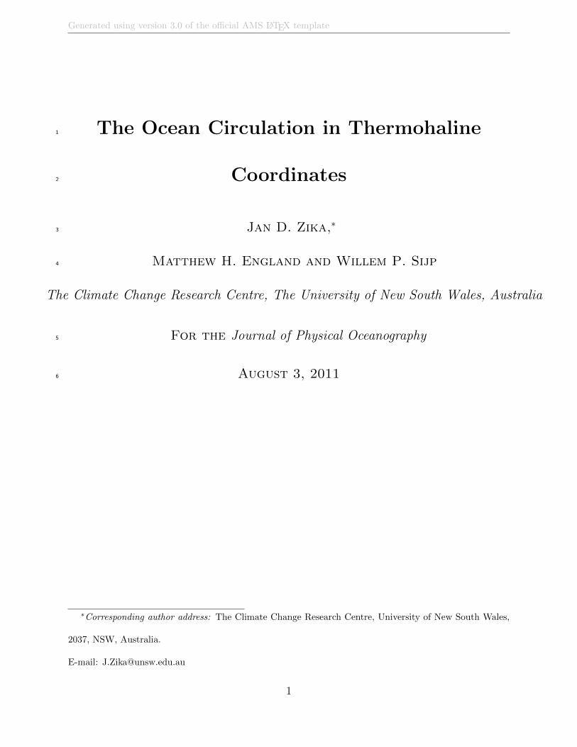
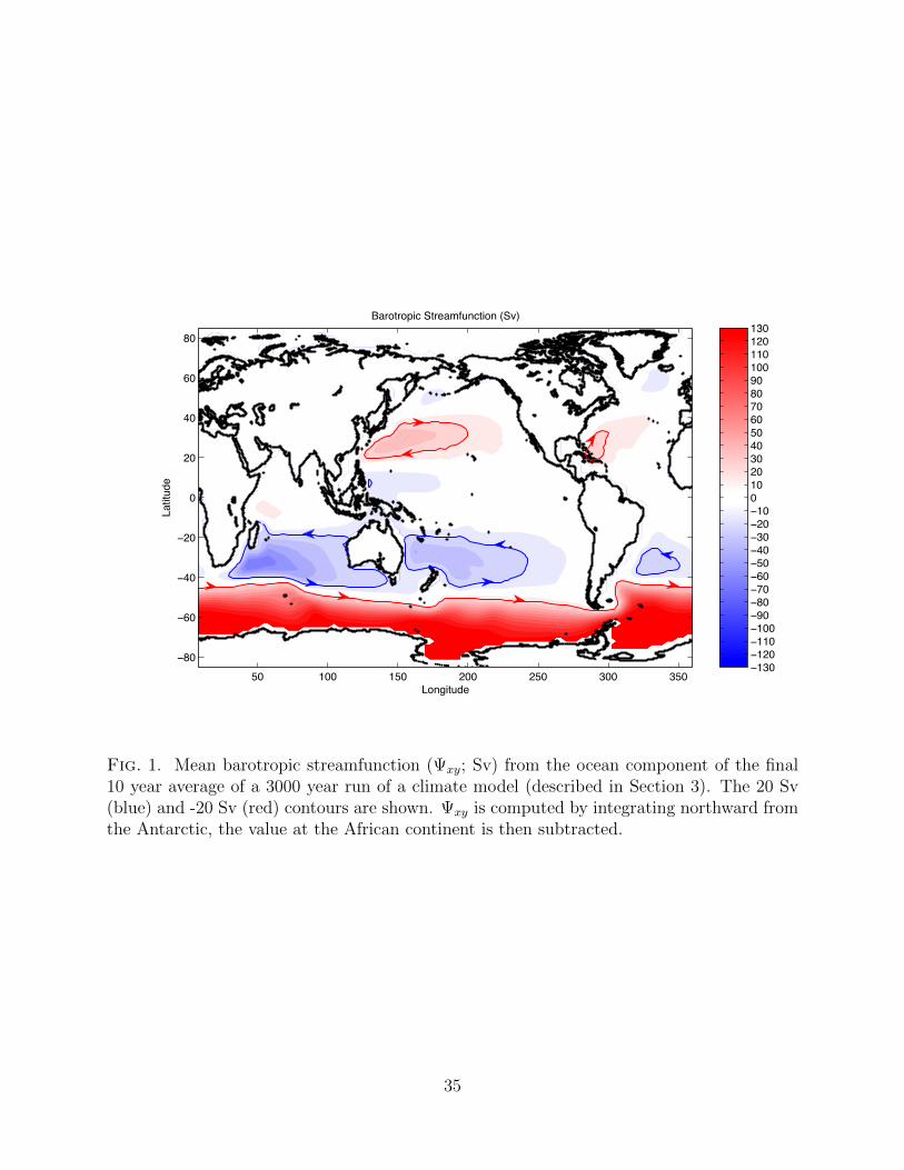
ψxy is commonly known as the barotropic streamfunction. The barotropic streamfunction105

for an intermediate complexity climate model (to be discussed in detail in Section 3) is plotted106

in Fig. 1. The barotropic streamfunction reveals the wind driven basin scale gyres, their107

boundary currents, and the pathway and strength of the Antarctic Circumpolar Current.108

5

Alternatively, integrating at constant depth and latitude, one can derive a meridional109

overturning streamfunction ψzy such that110

∂ψzy∂y

= −∫ x2

x1

w dx ;∂ψzy∂z

=

∫ x2

x1

v dx (4)

and again, so long as w = 0 at z = −H (e.g. below the deepest topography), ψzy can be111

diagnosed as:112

ψzy(y, z) = −∫ z

−H

∫ x2

x1

v(x, y, z′) dx dz′. (5)

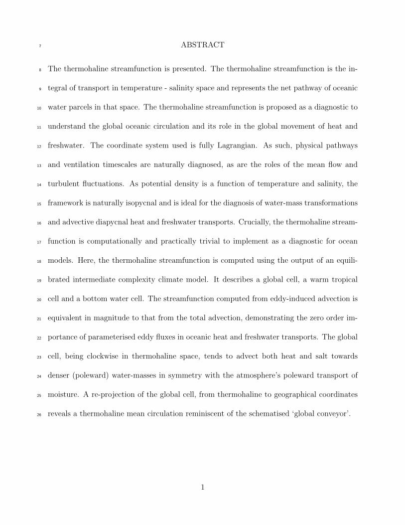
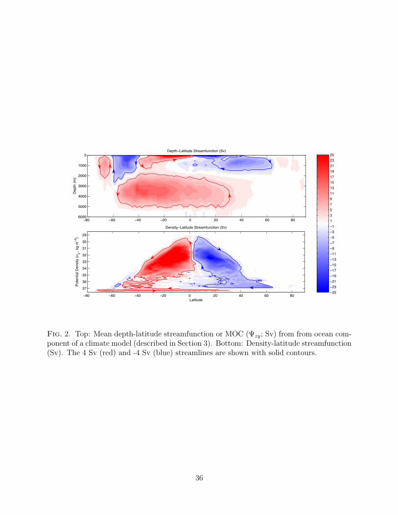
The meridional overturning streamfunction (MOC) for an intermediate complexity climate113

model is plotted in Fig. 2. The MOC reveals meridional cells linking the equatorial and114

poleward waters and the surface and deep waters. As discussed in Section 1, the MOC115

does not accurately represent the meridional exchanges of waters of different densities and116

temperatures. In order to diagnose such exchanges, and infer the processes which contribute117

to those exchanges, it is illuminating to compute a streamfunction as a function of latitude118

and a second, time evolving tracer. Following Ferrari and Ferreira (2011), we define a119

meridional streamfunction ψCy, for an arbitrary tracer C, such that120

ψCy =

∫ ∫C′≤C

v dx dz (6)

where∫ ∫

C′≤C dxdz is the area over a surface of constant latitude, where C ′ ≤ C. The121

streamfunction ψCy can be used to diagnose the advective meridional transport of C and to122

understand which mechanism give rise to that transport (Ferrari and Ferreira 2011).123

Equation (7) applied to an instantaneous velocity field gives an instantaneous streamfunc-124

tion. In this case the streamfunction represents not only the rate at which water parcels move125

from one concentration, C, to another, but also the rate at which iso-surfaces of constant126

6

C move in space. Averaging over some period ∆t we may diagnose a mean streamfunction127

ΨCy such that128

ΨCy =1

∆t

∫ t+∆t

t

∫ ∫C′≤C

v dx dz dt (7)

Here and throughout, time mean streamfunctions will be defined using a capital Ψ. Eule-129

rian mean and fluctuating components will later be distinguished using Ψ and Ψ′ respec-130

tively. As (Ferrari and Ferreira 2011) point out, if C is steady over the period ∆t, (i.e.131 ∫ t+∆t

t(dC/dt)dt = 0), then ΨCy represents the flow of water from one C value to another.132

Whether or not the flow is steady, ΨCy, can still be diagnosed, in the unsteady case it repre-133

sents both the transformation of water parcels and the movement of the tracer (Nurser and134

Marsh 1998).135

Here we compute the Ψyσ2 , that is, a streamfunction in potential density - latitude co-136

ordinates (σ2 being density referenced to 2000m depth; Fig. 2 b). The density-latitude137

streamfunction gives a complementary view of the circulation to the depth-latitude stream-138

function (Fig. 2a). In particular the Deacon Cell is reduced to 3-4 Sv in the density-latitude139

case. The parameterised eddy-induced velocity and zonal asymmetries allow a circulation to140

exist in the Southern Ocean in latitude-depth space without large exchanges of mass (den-141

sity) across latitude circles. In addition, the bottom water cell around Antarctica and the142

deep ’abyssal cell’ below 2000m depth are here linked together in one bottom water cell at143

densities greater than 37 kg m−3.144

What is not clear from the depth-latitude, nor the density latitude streamfunction, is145

the route taken by dense waters after they have sunk in formation regions such as the North146

Atlantic. Both diagnostics show a sinking around 60◦N. Where these waters eventually upwell147

7

and which geographical regions they transit through (either isopycnally or diapycnally) is148

unclear.149

b. A streamfunction in two general coordinates150

We seek a streamfunction which is not solely meridional, but can also encapsulate vertical151

and zonal motions as well. As such, we compute a streamfunction ψC1C2 in terms of two152

tracers, C1 and C2. Hence153

ψC1C2 =

∫C′

1≤C1|C2

u · nC2 dA (8)

where nC1 is the direction normal to a C2 iso-surface and∫C′

1≤C1|C2dA is the area over the154

C2 iso-surface where C ′1 ≤ C1. Again, the instantaneous ψC1C2 represents both the trans-155

formation of water parcels from different tracer concentrations and the adiabatic movement156

of tracer iso-surfaces (see Griffies 2007, pages 138-141 for a discussion of dia-surface flow).157

The mean streamfunction in the C1 − C2 coordinate is then158

ΨC1C2 =1

∆t

∫ t+∆t

t

∫C′

1≤C1|C2

u · nC1 dA dt (9)

In this study we will only consider cases where tracers are statistically steady. Interpretations159

of unsteady streamfunctions are left to future work.160

Note that a streamfunction ΨC1C2 could be formulated for iso-surfaces of constant C1161

where ΨC1C2 = −ΨC2C1 . Replacing C2 with the meridional coordinate y, (9) is equivalent to162

(7) as u ·ny = v. Indeed, one could also replace C1 with the vertical coordinate z and recover163

the mean of the latitude-depth overturning Ψyz (5; i.e. the MOC). Hence (9) represents a164

general equation for a streamfunction in two coordinates, whether in standard geographical165

8

coordinates or coordinates defined by time variable tracers.166

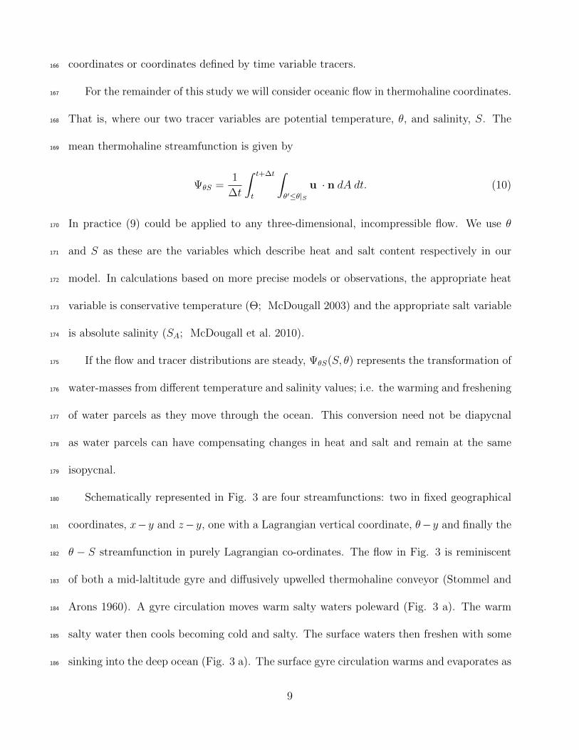
For the remainder of this study we will consider oceanic flow in thermohaline coordinates.167

That is, where our two tracer variables are potential temperature, θ, and salinity, S. The168

mean thermohaline streamfunction is given by169

ΨθS =1

∆t

∫ t+∆t

t

∫θ′≤θ|S

u · n dA dt. (10)

In practice (9) could be applied to any three-dimensional, incompressible flow. We use θ170

and S as these are the variables which describe heat and salt content respectively in our171

model. In calculations based on more precise models or observations, the appropriate heat172

variable is conservative temperature (Θ; McDougall 2003) and the appropriate salt variable173

is absolute salinity (SA; McDougall et al. 2010).174

If the flow and tracer distributions are steady, ΨθS(S, θ) represents the transformation of175

water-masses from different temperature and salinity values; i.e. the warming and freshening176

of water parcels as they move through the ocean. This conversion need not be diapycnal177

as water parcels can have compensating changes in heat and salt and remain at the same178

isopycnal.179

Schematically represented in Fig. 3 are four streamfunctions: two in fixed geographical180

coordinates, x−y and z−y, one with a Lagrangian vertical coordinate, θ−y and finally the181

θ − S streamfunction in purely Lagrangian co-ordinates. The flow in Fig. 3 is reminiscent182

of both a mid-laltitude gyre and diffusively upwelled thermohaline conveyor (Stommel and183

Arons 1960). A gyre circulation moves warm salty waters poleward (Fig. 3 a). The warm184

salty water then cools becoming cold and salty. The surface waters then freshen with some185

sinking into the deep ocean (Fig. 3 a). The surface gyre circulation warms and evaporates as186

9

it moves southward becoming warm and salty again. The deep portion warms and freshens187

via interior mixing as it upwells (Fig. 3 b). Averaging at constant latitude we see that this188

circulation transports warm water northward and cold water southward (Fig. 3 c). Averaging189

in temperature salinity space we see that, in this special case, both the gyre circulation and190

the diffusively upwelled overturning involve a circulation from warm and fresh to warm and191

salty, then to cold and salty, to cold and fresh and back to warm and fresh.192

Ocean models do not describe a continuous flow field and temperature and salinity dis-193

tributions but rather, a discretised approximation of it. The most common discretisation is194

one where the equations of motion and property conservation are solved on a grid defined195

by finite volumes. For each volume, a property concentration is assigned, as are transports196

across grid volume interfaces.197

Here we describe how ΨθS is calculated from a finite volume ocean model. Consider a198

model with 1 : N grid box interfaces and 1 : M discrete time steps. Volume fluxes, Uij,199

across all grid box interfaces, i, at time steps, j, are determined from the interface velocity200

and the interface area (e.g. U = [u∆y∆z; v∆x∆z;w∆x∆y] for longitudinal, latitudinal and201

vertical grid spacing ∆x, ∆y and ∆z respectively); and the respective temperatures at the202

interfaces θij and the salinities of the adjoining grid boxes S+ij and S−ij are stored in computer203

memory. Then, over all time steps the thermohaline streamfunction is computed using204

10

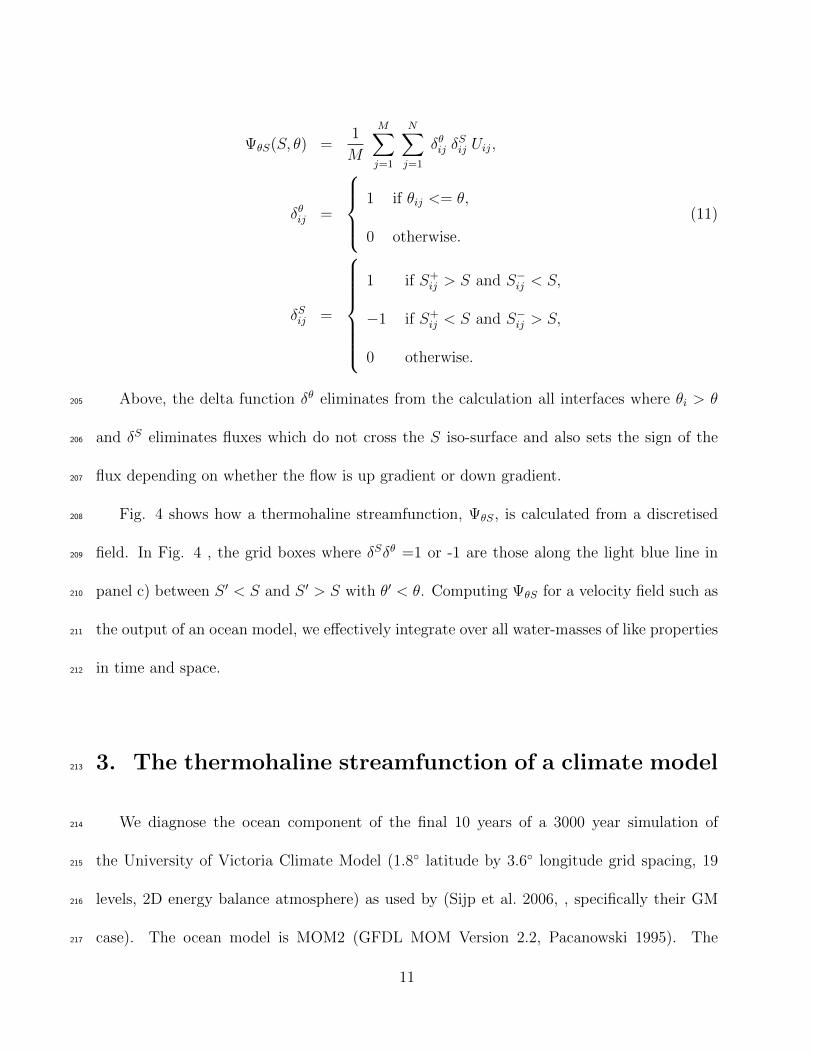
ΨθS(S, θ) =1

M

M∑j=1

N∑j=1

δθij δSij Uij,

δθij =

1 if θij <= θ,

0 otherwise.

(11)

δSij =

1 if S+

ij > S and S−ij < S,

−1 if S+ij < S and S−ij > S,

0 otherwise.

Above, the delta function δθ eliminates from the calculation all interfaces where θi > θ205

and δS eliminates fluxes which do not cross the S iso-surface and also sets the sign of the206

flux depending on whether the flow is up gradient or down gradient.207

Fig. 4 shows how a thermohaline streamfunction, ΨθS, is calculated from a discretised208

field. In Fig. 4 , the grid boxes where δSδθ =1 or -1 are those along the light blue line in209

panel c) between S ′ < S and S ′ > S with θ′ < θ. Computing ΨθS for a velocity field such as210

the output of an ocean model, we effectively integrate over all water-masses of like properties211

in time and space.212

3. The thermohaline streamfunction of a climate model213

We diagnose the ocean component of the final 10 years of a 3000 year simulation of214

the University of Victoria Climate Model (1.8◦ latitude by 3.6◦ longitude grid spacing, 19215

levels, 2D energy balance atmosphere) as used by (Sijp et al. 2006, , specifically their GM216

case). The ocean model is MOM2 (GFDL MOM Version 2.2, Pacanowski 1995). The217

11

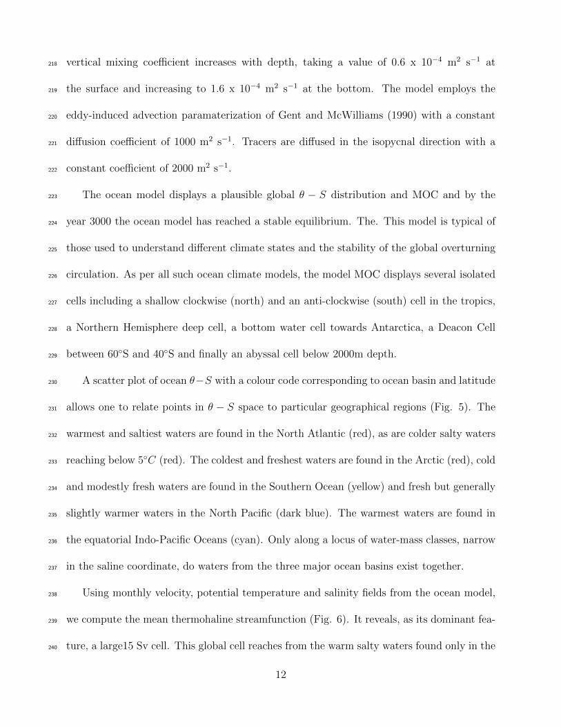
vertical mixing coefficient increases with depth, taking a value of 0.6 x 10−4 m2 s−1 at218

the surface and increasing to 1.6 x 10−4 m2 s−1 at the bottom. The model employs the219

eddy-induced advection paramaterization of Gent and McWilliams (1990) with a constant220

diffusion coefficient of 1000 m2 s−1. Tracers are diffused in the isopycnal direction with a221

constant coefficient of 2000 m2 s−1.222

The ocean model displays a plausible global θ − S distribution and MOC and by the223

year 3000 the ocean model has reached a stable equilibrium. The. This model is typical of224

those used to understand different climate states and the stability of the global overturning225

circulation. As per all such ocean climate models, the model MOC displays several isolated226

cells including a shallow clockwise (north) and an anti-clockwise (south) cell in the tropics,227

a Northern Hemisphere deep cell, a bottom water cell towards Antarctica, a Deacon Cell228

between 60◦S and 40◦S and finally an abyssal cell below 2000m depth.229

A scatter plot of ocean θ−S with a colour code corresponding to ocean basin and latitude230

allows one to relate points in θ − S space to particular geographical regions (Fig. 5). The231

warmest and saltiest waters are found in the North Atlantic (red), as are colder salty waters232

reaching below 5◦C (red). The coldest and freshest waters are found in the Arctic (red), cold233

and modestly fresh waters are found in the Southern Ocean (yellow) and fresh but generally234

slightly warmer waters in the North Pacific (dark blue). The warmest waters are found in235

the equatorial Indo-Pacific Oceans (cyan). Only along a locus of water-mass classes, narrow236

in the saline coordinate, do waters from the three major ocean basins exist together.237

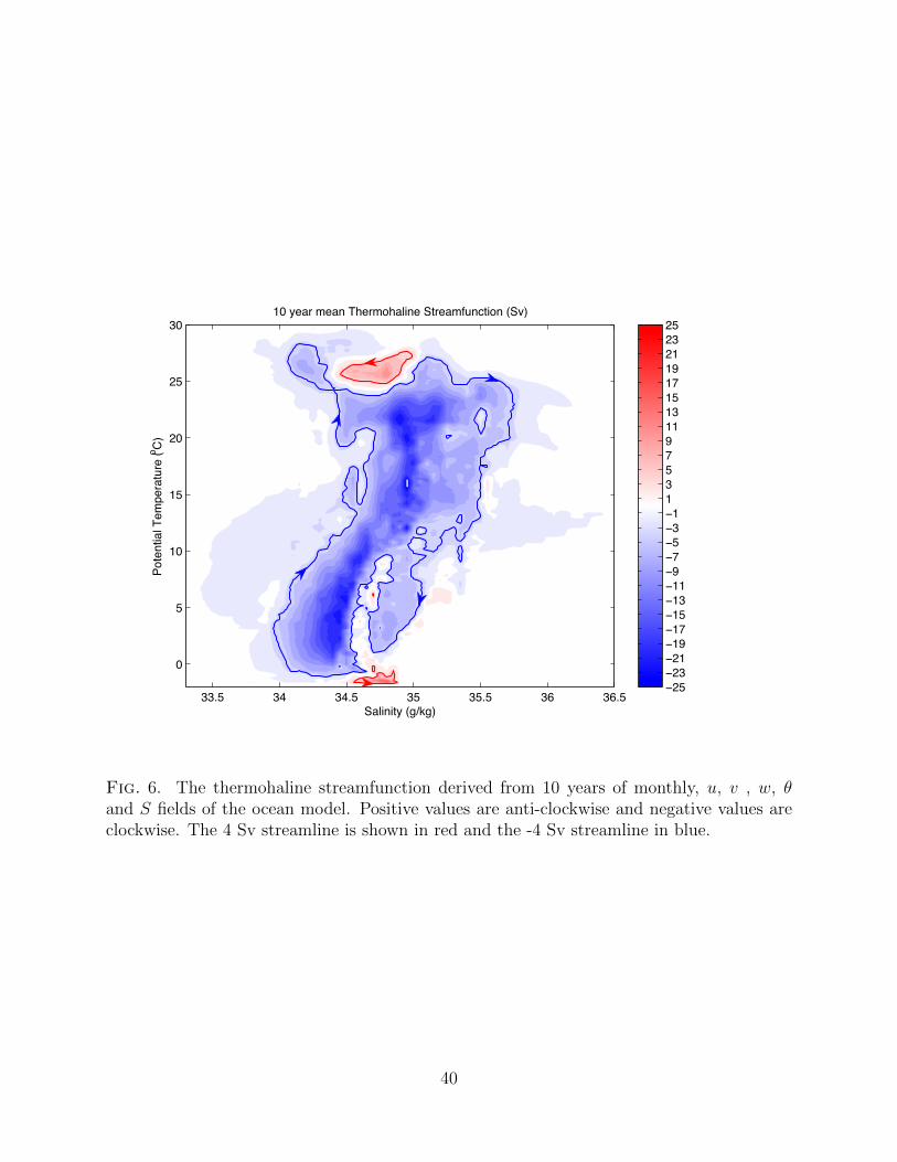
Using monthly velocity, potential temperature and salinity fields from the ocean model,238

we compute the mean thermohaline streamfunction (Fig. 6). It reveals, as its dominant fea-239

ture, a large15 Sv cell. This global cell reaches from the warm salty waters found only in the240

12

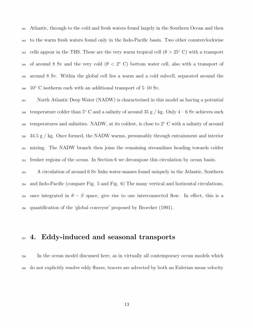
Atlantic, through to the cold and fresh waters found largely in the Southern Ocean and then241

to the warm fresh waters found only in the Indo-Pacific basin. Two other counterclockwise242

cells appear in the THS. These are the very warm tropical cell (θ > 25◦ C) with a transport243

of around 8 Sv and the very cold (θ < 2◦ C) bottom water cell, also with a transport of244

around 8 Sv. Within the global cell lies a warm and a cold subcell, separated around the245

10◦ C isotherm each with an additional transport of 5–10 Sv.246

North Atlantic Deep Water (NADW) is characterised in this model as having a potential247

temperature colder than 5◦ C and a salinity of around 35 g / kg. Only 4 – 6 Sv achieves such248

temperatures and salinities. NADW, at its coldest, is close to 2◦ C with a salinity of around249

34.5 g / kg. Once formed, the NADW warms, presumably through entrainment and interior250

mixing. The NADW branch then joins the remaining streamlines heading towards colder251

fresher regions of the ocean. In Section 6 we decompose this circulation by ocean basin.252

A circulation of around 6 Sv links water-masses found uniquely in the Atlantic, Southern253

and Indo-Pacific (compare Fig. 5 and Fig. 6) The many vertical and horizontal circulations,254

once integrated in θ − S space, give rise to one interconnected flow. In effect, this is a255

quantification of the ‘global conveyor’ proposed by Broecker (1991).256

4. Eddy-induced and seasonal transports257

In the ocean model discussed here, as in virtually all contemporary ocean models which258

do not explicitly resolve eddy fluxes, tracers are advected by both an Eulerian mean velocity259

13

(uEM) and an eddy-induced velocity (uGM) such that260

u = uEM + uGM . (12)

The eddy-induced velocity is prescribed using the scheme of Gent and McWilliams (1990).261

In the MOC, (uGM) is significant mainly in the Southern Ocean and North Atlantic where262

isopycnal slopes are very large. When computing the THS of Fig. 6, we used both the263

eddy-induced and Eulerian velocities and averaged these for each monthly field. We can264

now assess the influence of the Eulerian flow and the eddy-induced flow and the fluctuations265

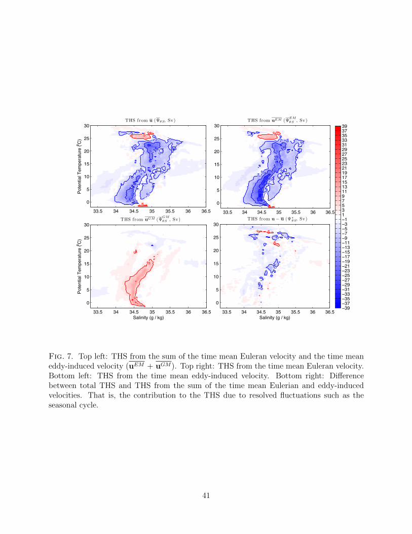
actually resolved by the model by making the following decomposition:266

ΨEM

θS (S, θ) =

∫θ′≤θ|S

uEM · n dA dt,

ΨGM

θS (S, θ) =

∫θ′≤θ|S

uGM · n dA dt (13)

where the overline represents an Eulerian average (i.e. ξ = 1∆t

∫ t+∆t

tξdt for some variable ξ).267

At its peak, the Eulerian mean contribution to the thermohaline streamfunction, ΨEM

θS ,268

is 39 Sv (Fig. 7 b). The global cell of the Eulerian plus eddy-induced THS is 15 Sv and269

peaks at 25 Sv in its sub-cells (Fig. 6). The Eulerian mean THS is compensated by an270

anti-clockwise circulation due to the eddy-induced velocity of around 5 - 10 Sv (Fig. 7b).271

This compensation occurs across a significant fraction of the water-mass classes covered by272

the global THS cell (-1◦C > θ > 15◦C and 34 g / kg > S > 35 g / kg). We find that, while273

uGM is small across most latitudes, it is large where water flows from one water-mass to274

another, particularly in the cooler fresher water-masses associated with the Southern Ocean.275

As above, the eddy-induced velocity is introduced to account for the effect of transient276

eddies not resolved on the 1.8◦ by 3.6◦ grid. The model does however, resolve fluctuations on277

14

seasonal and inter-annual timescales and hence we do expect a difference between ΨθS and278

ΨθS = ΨEM

θS + ΨGM

θS ; the difference being the role played by resolved temporal fluctuations279

(Ψ′θS, Fig. 7d). The major difference between the two is in the tropical waters (θ > 20◦C)280

and in the region linking the warm salty portion and the cold fresh portion of the global281

cell (θ ≈ 15◦C and S ≈ 35g/kg). The ocean model used here is known to display a robust282

seasonal cycle but small interannual fluctuations. It is thus likely that that in this model,283

and perhaps in the real ocean, seasonal fluctuations that contribute around 5 Sv of exchange284

between warm salty and cold fresh waters.285

5. Diapycnal fluxes and the symmetric diapycnal flux286

theorem287

By way of introduction to the idea of diagnosing the advective heat transport from a288

streamfunction, we again revisit Ferrari and Ferreira (2011) where their latitude-θ stream-289

function Ψy−θ can be used to diagnose the advective meridional heat transport (MHT) using290

MHT (y, θ) =

∫ ∞−∞

ρ0 cp Ψyθ dθ (14)

where ρ0 is a reference density and cp is the heat capacity of sea water. Equation (14)291

represents the flux of heat in the meridional direction due to advection, at the latitude y. In292

the case of the thermohaline streamfunction, ΨθS can be used to determine a heat function293

describing the flux of heat across isohalines and a salt function describing the flux of salt294

across isotherms.295

As potential density is a function of temperature and salinity, a heat function and salt296

15

function can also be defined, describing the flux of heat and salt across isopycnals. The total297

heat and salt transports across an isopycnal are given by298

FHeat(σ) = ρ0 cp

∫ ∞−∞

∂ΨθS

∂θθ dθ|σ + ρ0 cp

∫ ∞−∞

∂ΨθS

∂Sθ dS|σ, (15)

FSalt(σ) =

∫ ∞−∞

∂ΨθS

∂θS dθ|σ +

∫ ∞−∞

∂ΨθS

∂SS dS|σ. (16)

The salt transport can be converted into the more tangible ‘freshwater transport’, FFW ,299

in units of Sverdrups simply using FFW = −FSalt/S. Here we use S = 35 g / kg. The300

diapycnal heat and freshwater transports across potential density surfaces (σ0) from the301

ocean model simulation are shown in Fig. 8.302

For most isopycnal ranges, the ocean transports heat towards denser waters and freshwa-303

ter towards lighter waters. This is consistent with a balance between the ocean circulation304

and the atmosphere; the subtropical waters being associated with a heat flux into the ocean305

and a freshwater flux out of the ocean. The denser polar waters are associated with a heat306

flux out of the ocean and a freshwater flux in. Greatbatch and Zhai (1990) used observed307

meridional heat flux estimates and the ocean hydrography to estimate a global heat-function308

in terms of a diffusivity for temperature. Our analysis suggests that accurate estimates of309

atmosphere-ocean heat and freshwater fluxes could be used to estimate the thermohaline310

streamfunction in a similar way. This would effectively be a combination of the surface311

water-mass analysis method of Walin (1982) extended to 2 tracers and the tracer-contour312

framework of Zika et al. (2010) used to relate interior diabatic pathways to mixing.313

The sign of the diapycnal heat and salt flux is evident geometrically from the thermo-314

haline streamfunction itself. Clockwise cells advect heat and salt toward denser waters and315

16

anticlockwise cells advect heat and salt toward lighter waters (Fig. 9). This symmetry316

between downward heat and freshwater fluxes can be formally stated in the following.317

For most θ, S and pressure ranges of the ocean, density increases with increasing salinity318

and reducing temperature, i.e.319

dσ = −α ∂θ + β ∂S (17)

where α is a positive thermal expansion coefficient and β is a positive haline contraction320

coefficient. Here we will make the sole assumption that α/β is constant for each σ. Applying321

the chain rule to (15) we obtain322

FHeat(σ) = ρ0 cp [ΨθSθ]θ=∞θ=−∞ − ρ0 cp

∫ ∞−∞

ΨθS dθ|σ

+ρ0 cp [ΨθSS]S=∞S=−∞ − ρ0 cp

∫ ∞−∞

ΨθS∂θ

∂SdS|σ. (18)

As ΨθS = 0 outside the maximum and minimum salinities and temperatures323

FHeat(σ) = −ρ0 cp

∫ ∞−∞

ΨθS dθ|σ − ρ0 cp

∫ ∞−∞

ΨθS∂θ

∂SdS|σ. (19)

and likewise for the salt flux324

FSalt(σ) = −∫ ∞−∞

ΨθS dS|σ −∫ ∞−∞

ΨθS∂S

∂θdθ|σ. (20)

Now using (17; where dσ = 0) we find325

FHeat(σ) = −ρ0 cp

∫ ∞−∞

ΨθS dθ|σ − ρ0 cp

∫ ∞−∞

ΨθSβ

αdS|σ. (21)

FSalt(σ) = −∫ ∞−∞

ΨθS dS|σ −∫ ∞−∞

ΨθSα

βdθ|σ. (22)

and hence given we are assuming α/β is constant for constant σ the ratio of diapycnal326

advective heat flux to salt flux is simply327

FHeat(σ)

FSalt(σ)= ρ0 cp

β

α. (23)

17

The significance of (23), hereafter the diapycnal flux symmetry theorem, is that where328

there is a net advective heat flux across isopycnals by the statistically steady flow, salinity329

must be advected also. Hence freshwater must be advected in the opposite direction. So330

where the ocean advects heat toward denser water-masses, it must advect freshwater towards331

lighter water-masses.332

In an ongoing study, we are investigating whether the diapycnal flux symmetry theorem333

has broader implications for global heat and freshwater transports. It may be the case that334

this theorem places constraints on the relationship between atmospheric moisture transport335

and ocean heat transport.336

6. Thermohaline transit time337

Given the thermohaline streamfunction and estimates of the mean gradients of temper-338

ature and salinity, it is possible to gain a measure of the time taken for a water parcel to339

make a full circuit in θ − S space. We name this measure the thermohaline transit time,340

TθS(Ψ). As we discuss in the next Section, individual water parcels, even in the absence of341

dispersion, do not complete entire ‘loops’ in θ−S space, as with any three dimensional flow.342

However, the concept of transit time is still insightful as it gives a measure of the minimum343

time for a water parcel to be advected in this fully Lagrangian co-ordinate system.344

For a fluid parcel following streamline in θ − S space, the time increment, dt|Ψ, for a345

given θ and S increments ∂θ|Ψ and ∂S|Ψ is346

dt|Ψ =Dt

Dθ∂θ|Ψ +

Dt

DS∂S|Ψ. (24)

18

That is, the time taken for a a fluid parcel to get between two points along a streamline347

separated by ∂θ|Ψ and ∂S|Ψ, depends on both the rate of change of temperature following the348

the fluid parcel Dθ/Dt, and the rate of change of salinity following the fluid parcel DS/Dt.349

If θ and S are statistically steady, in order for a fluid parcels to change its temperature and350

salinity, it must be advected to somewhere with a different temperature and salinity such351

that352

Dθ

Dt= u · ∇θ ;

DS

Dt= u · ∇S. (25)

By computing ΨθS from (10) we have naturally computed an average of both components of353

the velocity needed in (25) as (10) can be written354

∆Ψ|S =1

∆t

∫ t+∆t

t

∫ θ+∆θ

θ

u · ∇θ|∇θ| dAS; (26)

∆Ψ|θ =1

∆t

∫ t+∆t

t

∫ S+∆S

S

u · ∇S|∇S| dAθ. (27)

Assuming the absolute gradients |∇θ| and |∇S| do not vary greatly in time or across the355

areas dAS and dAθ respectively, we can make the following approximation:356

∆Ψ|S∆AS

=⟨

u·∇θ|∇θ|

⟩≈ < u · ∇θ >

< |∇θ| > (28)

∆Ψ|θ∆Aθ

=⟨

u·∇S|∇S|

⟩≈ < u · ∇S >

< |∇S| > . (29)

Above, the angular brackets (< >) represent the average in time and over an isotherm357

between S and S+ ∆S and the average over an isohaline between θ and θ+ ∆θ respectively.358

From the time mean θ and S fields of the model, we can compute < |∇θ| > and < |∇S| >359

simply by averaging the gradients across the areas dAS and dAΘ. Thus from (25) we have360

Dθ

Dt≈ ∆Ψ|S

∆AS< |∇θ| >;

DS

Dt≈ ∆Ψ|θ

∆Aθ< |∇S| > . (30)

19

Substituting into (24) then yields361

dt|ψ ≈1

∆Ψ|S∆AS

< |∇θ| >∂θ|Ψ +

1∆Ψ|θ∆Aθ

< |∇S| >∂S|Ψ. (31)

One can then estimate the time rate of change following the ΨθS streamline by integrating362

(31) such that the total thermohaline transit time, TθS(Ψ), is363

TθS(Ψ) =

∮dt|Ψ

≈∮

1∆Ψ|S∆AS

< |∇θ| >∂θ|Ψ +

∮1

∆Ψ|θ∆Aθ

< |∇S| >∂S|Ψ. (32)

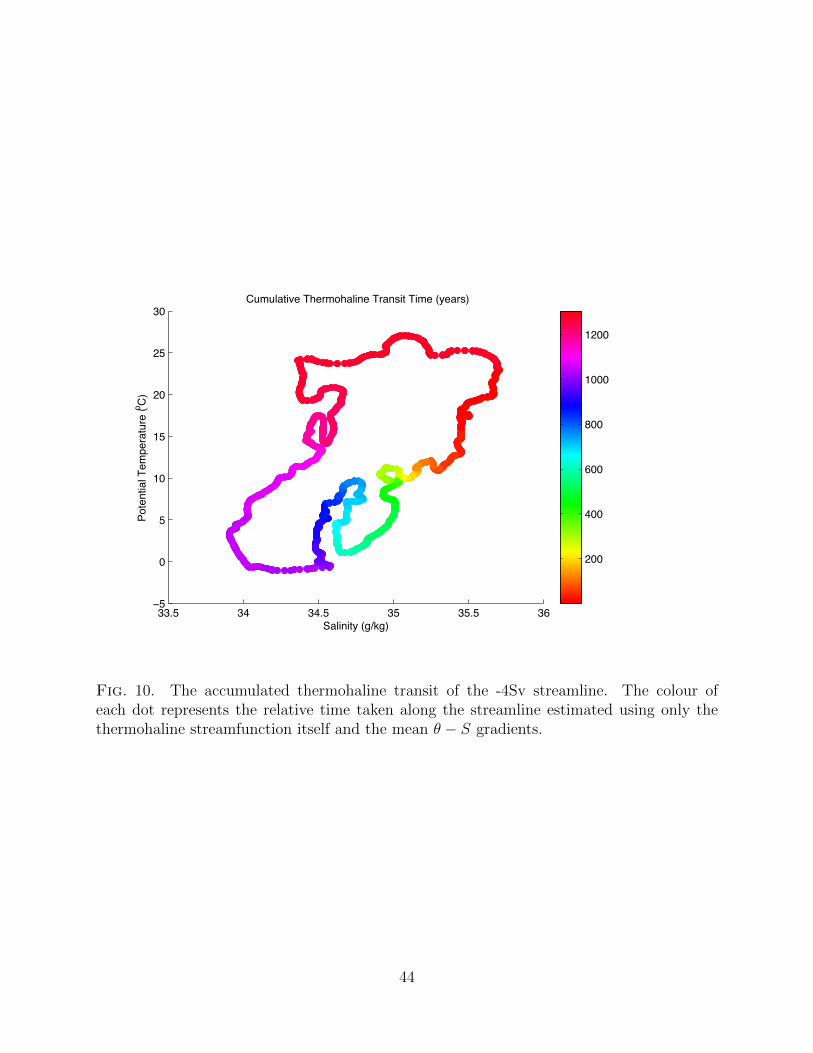
We calculate TθS by following the longest -4 Sv streamline in θ− S space (Fig. 10). The364

full circuit takes 1,350 years using (32). The cumulative time taken along the contour shows365

how the fluid moves from the warmest freshest waters around 25◦ C and 34.4 g / kg to the366

cool high saline waters at 10◦ C and 35.5 g / kg in a relatively short time-scale of 100 years367

or so. This short time-scale is likely to be because of the strong, near surface wind driven368

circulation allowing rapid transitions between different water-masses. The transit from this369

water-mass (NADW) to the cold fresh waters around 0◦ C and 34.5 g / kg, a relative short370

distance in θ − S space, takes the considerable majority of the remaining 1250 year transit.371

These dense water-masses are found only in the deep ocean where advection is weak and372

temperature and salinity gradients are large meaning water-mass transitions occur gradually.373

The thermohaline transit time of THS contours are shown in Fig. 11. In each case we374

take the longest streamline for a given transport value. The tropical cell, defined as anti-375

clockwise cells warmer than 10oC, has the shortest transit times of order 20 years. For the376

global cell and it’s subcells, the transit times range from hundreds of years and asymptote377

20

to around 1500 years for the -2 Sv contour. We do not discern between subcells in the378

warmer or colder portions of the global cell. The longest bottom water cell transit times are379

equivalent to global cell at order 1500 years. Increased resolution of the THS in θ− S space380

may change the bottom water transit times estimated here.381

7. Basin specific flow and water-mass pathways382

Here we address whether streamlines in thermohaline space correspond to pathways of383

individual water parcels or whether this circulation is simply the accumulation of many,384

geographically independent cells. To answer this question we start by investigating the385

nature of the THS in separate geographical regions where such a separation is possible.386

The North Atlantic is generally saltier than the Indian and Pacific basins. However the387

two share waters of like θ−S properties. Looking at the maximum temperatures and salinities388

along the sections which separate the Atlantic from the Indo-Pacific, we can determine θ−S389

ranges which are either ‘wholly’ within the Atlantic or ‘wholly’ within the Indo-Pacific, and390

of course, not in the Southern Ocean. That is, although like θ − S properties may exist in391

both basins, they are not geographically linked at any time. Any volume transport from392

Atlantic water to Indo-Pacific water must occur through some other intermediary θ − S393

range.394

The θ − S ranges we choose for this strictly ’non Southern Oceanwater are S > 35g/kg,395

S > 34.8g/kg and θ > 21.5oC or S < 34.8g/kg and θ > 16oC (i.e. only those regions in θ−S396

space which have green or red contours in Fig. 12) . Any water in that range is either in the397

Atlantic, or in the Indo-Pacific, but not in the Southern Ocean. Hence, a streamfunction can398

21

be defined independently by integrating form θ =∞ back to the edge of this domain in θ−S399

space. The result and the geographical domain of the two water-masses is shown in Fig. 12.400

The streamlines for the Indo-Pacific are shown in green and the Atlantic in red. Clearly the401

wide, anvil shape of the global THS is the result of a combination of a fresher Indo-Pacific402

branch and a saltier Atlantic branch. The warmest saltiest waters only exist in the Atlantic403

and the coldest freshest waters only exist in the the Indo-Pacific. The Indo-Pacific takes404

freshwater from the deep or southern waters and returns them as saltier waters while the405

Atlantic takes intermediate salinity waters and returns them as high salinity waters.406

The same decomposition as is done for the warmest waters by ocean basin can be done407

for the coldest freshest waters by hemisphere. Cold fresh water exists in both the Southern408

Ocean and the Arctic/North Pacific. However, no cold fresh water exists around the Equator.409

Hence we can partition the two. Specifically, we compute a streamfunction only for waters410

with θ < 12oC and S < 34.5g/kg for each hemisphere. The resulting Southern Ocean411

streamfunction is almost the same as that derived from the sum of both the Northern412

and Southern Hemispheres, demonstrating the dominant role of the Southern Ocean in the413

circulation in this θ − S range.414

An interpretation of the global water-mass pathway thus emerges of water moving from415

the Atlantic to the Southern Ocean and into the Pacific. We now attempt to track this416

pathway more precisely by following a streamline from one basin to the next. We take the417

THS plotted in Fig. 12 and follow the θ − S values corresponding to the longest -4 Sv418

streamline. We start with the freshest point in the Atlantic on this contour. This contour is419

tracked until the edge of the Atlantic water-mass is reached at S = 35g/kg. At this point the420

Atlantic streamfunction matches the global one. Continuing along the global streamline to421

22

S = 34.5g/kg the global THS matches almost perfectly with the Southern Ocean and again422

to θ = 12◦C where it matches with the Pacific. Although one could continue indefinitely, we423

stop where this streamline reaches θ = 21.5oC and S > 34.5g/kg. By allowing streamlines424

to transit from one basin to the next, the circulation is no longer closed and no one cell425

exists in a unique sense.426

In order to determine the possible geographical route of water parcels along this ther-427

mohaline pathway we colour water-masses in the ocean according to their location in θ − S428

space. For each point along the contour, a colour is chosen corresponding to the ‘distance’429

along the contour; distance being in θ − S space, not geographical space. The colour is430

then used to label the actual points in the ocean which have that temperature and salinity.431

The resulting analysis is shown in Fig. 13. Following the pathway as it moves from the432

surface Atlantic to the North Atlantic, then down into the deep ocean, and eventually up433

into the Southern Ocean and out into the North Pacific, reveals a pathway reminiscent of434

the schematic diagrams of the thermohaline circulation, first depicted by Gordon (1986).435

An important difference between the conveyor of Gordon (1986) and Broecker (1991)436

and that revealed by Fig. 13 is that the model diagnosed THS transits through the surface437

waters of the Southern Ocean with significant transformation of θ − S properties. This438

is despite the meridional overturning in density space showing North Atlantic Deep Water439

upwelling diapycnally at mid-latitudes (Fig. 2). This suggests that waters are exchanged440

meridionally at constant density, but enter and exit with different temperatures and salinities441

(i.e. different spiciness).442

23

8. Summary and conclusions443

The circulation of a global ocean model has been presented in temperature salinity coor-444

dinates for the first time. The resulting thermohaline streamfunction, the THS, distils the445

ocean circulation into three distinct cells: a tropical warm cell, a global cell and an Antarctic446

Bottom Water cell. Many of the streamlines (around 4-5 Sv) of the global cell link the cold447

and salty waters of the North Atlantic to the warm fresh waters of the Indo-Pacific Ocean,448

providing a quantification of the models ‘global conveyor’. In addition, a number of novel449

advantages of computing a thermohaline streamfunction are revealed.450

First, the THS can be used to diagnose the role of resolved and parameterised transient451

fluxes in water-mass transformation zones. Parameterised transient eddy fluxes are found452

to be leading order across the majority of water-mass classes. Averaging in thermohaline453

space provides a unique Lagrangian framework in which the role of diabatic processes and454

parameterised fluxes are highlighted.455

Second, once the circulation is averaged in thermohaline coordinates, diapycnal heat and456

salt transports are easily quantified. Clockwise cells in thermohaline space flux heat and salt457

towards denser waters and anti-clockwise cells flux heat and salt towards lighter waters. This458

symmetry between diapycnal heat and salt fluxes is formalised with the symmetric diapycnal459

flux theorem (23). In our model, heat and salt are transported from light waters to dense460

waters by the clockwise global cell. Heat and salt are transported from light waters associated461

with sub-tropical latitudes to denser waters associated with polar regions. This poleward462

salt transport is in symmetry with the atmosphere’s poleward transport of freshwater at463

subtropical to subpolar latitudes.464

24

A measure of the transit time of the global conveyor, the thermohaline transit time, is465

easily quantified from the THS. The thermohaline transit time in our model is 1350 years for466

typical streamlines associated with the the conveyor. Such a simple diagnostic may prove467

useful in comparing the ventilation time of various models, especially in cases where the468

incorporation of more involved tracer diagnostics is prohibitive.469

Separating the THS by region, the Southern Ocean is found to dominate the coolest and470

freshest water-masses. The THS trajectory from cool fresh waters to cool and salty waters is471

the sum of both a fresher tropical/subtropical branch in the Indian and Pacific Oceans and472

a saltier tropical to subpolar branch in the Atlantic Ocean. The sum of these three branches473

reveals a globally interconnected circulation.474

A major difference between the global conveyor of this model and the schematic view of475

Gordon (1986) and Broecker (1991) is that most of the diagnosed THS (-5 to -15 Sv; narrow476

core of the THS in Fig. 6) occurs at the surface rather than in deep waters. In addition477

almost all streamlines (0 to -15 Sv) transit through the Southern Ocean. This is despite478

the majority of diapycnal upwelling in the model occurring in the abyssal ocean (Fig. 2).479

This implies that even a density space overturning, driven by interior diapycnal mixing, may480

still transit through the Southern Ocean in order for global balances of heat and salt to be481

maintained.482

9. Acknowledgements483

This work was supported by the Australian Research Council. We thank Steven Griffies484

for providing helpful comments on a draft of this manuscript.485

25

486

REFERENCES487

Blanke, B., M. Arhan, and S. Speich, 2006: Salinity changes along the upper limb of the488

Atlantic thermohaline circulation. Geophysical Research Letters, 33, 6609.489

Boccaletti, G. R., R. Ferrari, A. Adcroft, D. Ferreira, and J. Marshal, 2005: The vertical490

structure of ocean heat transport. Geophysical Research Letters, 32, 10 603–10 606.491

Broecker, W. S., 1991: The Great Ocean Conveyor. Oceanography, 4, 79–89.492

Cuny, J., P. B. Rhines, P. P. Niiler, and S. Bacon, 2002: Labrador sea boundary currents and493

the fate of the irminger sea water. Journal of Physical Oceanography, 32 (2), 627–647.494

Davis, R. E., R. de Szoeke, D. Halpern, and P. Niiler, 1981: Variability in the upper ocean495

during MILE. Part I: The heat and momentum balances. Deep–Sea Research, 28, 1427–496

1452.497

Deacon, G. E. R., 1937: The hydrology of the Southern Ocean, Vol. 15, 3–122. Cambridge498

University Press,.499

Doos, K. and D. Webb, 1994: The Deacon cell and other meridional cells of the Southern500

Ocean. Journal of Physical Oceanography, 24, 429–442.501

Ferrari, R. and D. Ferreira, 2011: What processes drive the ocean heat transport. Ocean502

Modelling, 38, 171–186.503

26

Gent, P. R. and J. C. McWilliams, 1990: Isopycnal mixing in ocean circulation models.504

Journal of Physical Oceanography, 20, 150–155.505

Gordon, A. L., 1986: Interocean exchange of thermocline water. Journal of Geophysical506

Research, 91, 5037–5046.507

Gordon, A. L., 1991: The role of thermohaline circulation in global climate change. In:508

LamontDoherty Geological Observatory 1990 and 1991 Report. Tech. rep., LamontDoherty509

Geological Observatory of Columbia University, Palisades, New York, 44-51 pp.510

Greatbatch, R. J. and X. Zhai, 1990: The generalized heat function. Geophysical Research511

Letters, 34, L21 601.512

Griffies, S., 2007: Fundamentals of ocean climate models. Princeton University Press, 230pp513

pp.514

Kuhlbrodt, T. A., M. Griesel, A. Montoya, A. Levermann, M. Hofmann, and S. Rahmstorf,515

2007: On the driving processes of the Atlantic meridional overturning circulation. Rev.516

Geophys., 45, doi:10.1029/2004RG000166.517

Manabe, S., K. Bryan, and M. J. Spelman, 1990: Transient response of a global ocean-518

atmosphere model to a doubling of atmospheric carbon dioxide. Journal of Physical519

Oceanography, 20 (5), 722–749.520

Marsh, R., S. A. Josey, A. J. G. de Nurser, B. A. Cuevas, and A. C. Coward, 2005: Water521

mass transformation in the north atlantic over 1985-2002 simulated in an eddy-permitting522

model. Ocean Science, 1 (2), 127–144.523

27

McDougall, T. J., 2003: Potential enthalpy: A conservative oceanic variable for evaluating524

heat content and heat fluxes. Journal of Physical Oceanography, 33, 945–963.525

McDougall, T. J., D. R. Jackett, and F. J. Millero, 2010: An algorithm for estimating526

Absolute Salinity in the global ocean. submitted to Ocean Science. Ocean Sci. Discuss.,527

6, 215–242.528

Munk, W. H. and K. Wunsch, 1998: Abyssal recipes II: Energetics of tidal and wind mixing.529

Deep–Sea Research, 45, 1977–2010.530

Nurser, A. J. G. and M.-M. Lee, 2004: Isopycnal averaging at constant height. Part I: The531

Formulation and a case study. Journal of Physical Oceanography, 34, 2721–2739.532

Nurser, A. J. G. and R. Marsh, 1998: Water mass transformation theory and the meridional533

overturning streamfunction. International WOCE newsletter, 31, 36–38.534

Nycander, J., J. Nilsson, K. Doos, and G. Bromstrom, 2007: Thermodynamic analysis of535

Ocean Circulation. Journal of Physical Oceanography, 37, 2038–2052.536

Pacanowski, R., 1995: MOM2 Documentation Users Guide and Reference Manual: GFDL537

Ocean Group Technical Report. Tech. rep., NOAA, GFDL, Princeton., 232 pp.538

Richardson, P. L., 2008: On the history of meridional overturning schematic diagrams.539

Progress in Oceanography, 76, 466–486.540

Schmitz, W. J., Jr., 1996: On the world ocean circulation. Volume I: Some global fea-541

tures/North Atlantic circulation. Tech. Rep. WHOI–96–03, Woods Hole Oceanographic542

Institute, 140 pp.543

28

Sijp, W. P., M. Bates, and M. H. England, 2006: Can isopycnal mixing control the stability544

of the Thermohaline Circulation in ocean climate models? Journal of Climate, 19, 5637–545

5651.546

Stommel, H. and A. B. Arons, 1960: On the abyssal circulation of the worlds ocean– II. An547

idealized model of circulation pattern and amplitude in oceanic basins. Deep–Sea Research,548

6, 140–154.549

Walin, G., 1982: On the relation between sea–surface heat flow and thermal circulation in550

the ocean. Tellus, 34, 187–195.551

Wust, G., 1935: Die stratosphare des Atlantischen Ozeans. Wissenschaftliche Ergebnisse der552

Deutschen Atlantischen Expedition auf dem Forschungs und Vermessungsschiff, Meteor553

1925–1927, Gruyter & Co.,, 109–288.554

Zika, J. D. and T. J. McDougall, 2008: Vertical and lateral mixing processes deduced from the555

Mediterranean Water signature in the North Atlantic. Journal of Physical Oceanography,556

38, 164–176.557

Zika, J. D., T. J. McDougall, and B. M. Sloyan, 2009a: A tracer-contour inverse method for558

estimating ocean circulation and mixing. Journal of Physical Oceanography, 40, 2647.559

Zika, J. D., T. J. McDougall, and B. M. Sloyan, 2010: Weak mixing in the eastern North At-560

lantic: An application of the tracer-contour inverse method. Journal of Physical Oceanog-561

raphy, 40, 1881–1893.562

Zika, J. D., B. M. Sloyan, and T. J. McDougall, 2009b: Diagnosing the Southern Ocean563

Overturning from tracer fields. Journal of Physical Oceanography, 39, 29262940.564

29

Zika, J. D. e. a., 2011: Vertical Eddy Fluxes in the Southern Ocean. Journal of Physi-565

cal Oceanography, Submitted. Preprint available at http://hal.archives–ouvertes.fr/hal–566

00592 075/en/.567

30

List of Figures568

1 Mean barotropic streamfunction (Ψxy; Sv) from the ocean component of the569

final 10 year average of a 3000 year run of a climate model (described in570

Section 3). The 20 Sv (blue) and -20 Sv (red) contours are shown. Ψxy571

is computed by integrating northward from the Antarctic, the value at the572

African continent is then subtracted. 35573

2 Top: Mean depth-latitude streamfunction or MOC (Ψzy; Sv) from from ocean574

component of a climate model (described in Section 3). Bottom: Density-575

latitude streamfunction (Sv). The 4 Sv (red) and -4 Sv (blue) streamlines are576

shown with solid contours. 36577

3 Schematic describing four streamfunction diagnostics: a) barotropic stream-578

funciton showing horizontal motion, b) meridional overturning streamfunction579

showing vertical motion, c) temperature-latitude streamfunction showing net580

effect of horizontal motion in transporting heat meridionally and d) thermo-581

haline streamfunction showing net effect of all motion in transporting water582

from regions of different temperatures and salinities. Overlaid in a), b) and583

d) are schematic isolines of constant potential temperature and salinity (at584

the surface in a) and zonally averaged in b). 37585

31

4 Schematic describing the way the thermohaline streamfunction is computed586

from the output of a finite volume ocean model. Model grid boxes are defined587

on some native coordinate (e.g. x and y, or y and z) by their salinity (a)588

and potential temperature (b). Where potential temperature θ′ < θ all fluxes589

are summed across grid box interfaces from salinity S ′ < S to S ′ > S in the590

native coordinate (c). Summing these fluxes, a thermohaline streamfunction591

at (θ, S) is determined and represented in thermohaline coordinates (d). 38592

5 Scatter plot of potential temperature and salinity from the mean state of the593

ocean model. Each grid box is represented by one dot in θ − S space. The594

colour of each dot corresponds to its latitude and basin using the colour code595

shown in the insert. 39596

6 The thermohaline streamfunction derived from 10 years of monthly, u, v ,597

w, θ and S fields of the ocean model. Positive values are anti-clockwise and598

negative values are clockwise. The 4 Sv streamline is shown in red and the -4599

Sv streamline in blue. 40600

7 Top left: THS from the sum of the time mean Euleran velocity and the time601

mean eddy-induced velocity (uEM + uGM). Top right: THS from the time602

mean Euleran velocity. Bottom left: THS from the time mean eddy-induced603

velocity. Bottom right: Difference between total THS and THS from the604

sum of the time mean Eulerian and eddy-induced velocities. That is, the605

contribution to the THS due to resolved fluctuations such as the seasonal cycle. 41606

32

8 a) Thermohaline Streamfunction (THS, ΨθS) as in Fig 6 but with contours607

of surface referenced potential density (σ0) overlaid. b) Diapycnal heat and608

c) diapycnal freshwater flux from the ocean model computed directly from609

the THS. The freshwater flux is simply computed as Fsalt/35g/kg. The total610

(solid), Eulerian (dashed) and eddy-induced (dotted) components are shown.611

Consistent with the symmetric diapycnal flux theorem (23), a positive heat612

flux corresponds to a negative freshwater flux throughout. 42613

9 Schematic describing the geometric relationship between the THS and diapy-614

cnal heat and salt fluxes. If water is advected toward denser waters on the615

warmer-saltier parts of an isopycnal surface (σ; left) this appears as a clock-616

wise circulation in θ − S space (right). As the same trajectory has different617

temperatures as it crosses the same isopycnal surface it represents a net pos-618

itive diapycnal transport of heat and salt. The circulation shown in physical619

space (left) can be both a horizontal (e.g. gyre in x-y space) circulation where620

this diapycnal transport is balanced by surface heating, cooling and evapo-621

ration minus precipitation and/or a vertical overturning (in z-y space) where622

the transport is balanced by interior mixing or nonlinear processes. 43623

10 The accumulated thermohaline transit of the -4Sv streamline. The colour of624

each dot represents the relative time taken along the streamline estimated625

using only the thermohaline streamfunction itself and the mean θ−S gradients. 44626

33

11 The thermohaline transit time of the longest THS streamlines in θ − S space627

(i.e the longest streamlines in Fig. 6 for each transport). Shown are transit628

times for the global cell (green), the bottom water cell (temperatures below629

10oC), and the tropical cell contours (longest positive streamlines with tem-630

peratures above 10oC). The Antarctic Bottom Water transit times may be631

underestimated due to interpolation onto a coarse θ − S grid. 45632

12 The thermohaline streamfunction (THS) for various oceanic regions. Shown633

are: THS for water-masses found only in the Indian and Pacific basins (green;634

green volume in insert), water-masses found only in the Atlantic (red) and635

finally water-masses found only in the Southern Ocean (blue). 46636

13 A thermohaline pathway projected into physical space. The -4 Sv THS con-637

tour is followed from the Atlantic water-masses (red in Fig. 12) to the South-638

ern Ocean (blue in Fig. 12) and then finally to the Indo-Pacific water-masses639

(bottom right panel). At points equally spaced in θ − S space along the640

contour, a colour is chosen to represent water-masses with those water-mass641

properties (bottom right panel). All grid boxes in the corresponding region642

with potential temperatures and salinities within 0.1◦C and 0.05 g / kg re-643

spectively of that point in θ − S space are then assigned the colour of that644

point. Top panel shows all grid boxes above 300m. Middle panel: all grid645

boxes below 300m. Bottom left panel: only Altantic grid boxes. Bottom646

middle panel: Indo-Pacifc grid boxes. 47647

34

130120110100908070605040302010

0102030405060708090100110120130

Longitude

Latit

ude

Barotropic Streamfunction (Sv)

50 100 150 200 250 300 35080

60

40

20

0

20

40

60

80

Fig. 1. Mean barotropic streamfunction (Ψxy; Sv) from the ocean component of the final10 year average of a 3000 year run of a climate model (described in Section 3). The 20 Sv(blue) and -20 Sv (red) contours are shown. Ψxy is computed by integrating northward fromthe Antarctic, the value at the African continent is then subtracted.

35

Dep

th (m

)

Depth Latitude Streamfunction (Sv)

80 60 40 20 0 20 40 60 80

0

1000

2000

3000

4000

5000

6000

252321191715131197531

135791113151719212325

Latitude

Pote

ntia

l Den

sity

(2 ,

kg m

3 )

Density Latitude Streamfunction (Sv)

80 60 40 20 0 20 40 60 80

29

30

31

32

33

34

35

36

37

Fig. 2. Top: Mean depth-latitude streamfunction or MOC (Ψzy; Sv) from from ocean com-ponent of a climate model (described in Section 3). Bottom: Density-latitude streamfunction(Sv). The 4 Sv (red) and -4 Sv (blue) streamlines are shown with solid contours.

36

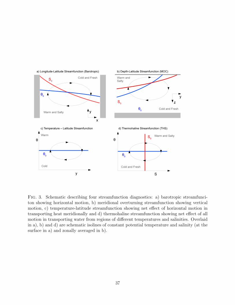
Fig. 3. Schematic describing four streamfunction diagnostics: a) barotropic streamfunci-ton showing horizontal motion, b) meridional overturning streamfunction showing verticalmotion, c) temperature-latitude streamfunction showing net effect of horizontal motion intransporting heat meridionally and d) thermohaline streamfunction showing net effect of allmotion in transporting water from regions of different temperatures and salinities. Overlaidin a), b) and d) are schematic isolines of constant potential temperature and salinity (at thesurface in a) and zonally averaged in b).

37

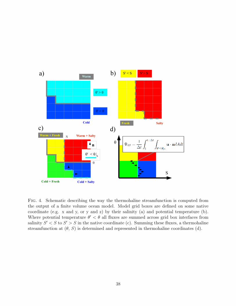
Fig. 4. Schematic describing the way the thermohaline streamfunction is computed fromthe output of a finite volume ocean model. Model grid boxes are defined on some nativecoordinate (e.g. x and y, or y and z) by their salinity (a) and potential temperature (b).Where potential temperature θ′ < θ all fluxes are summed across grid box interfaces fromsalinity S ′ < S to S ′ > S in the native coordinate (c). Summing these fluxes, a thermohalinestreamfunction at (θ, S) is determined and represented in thermohaline coordinates (d).

38

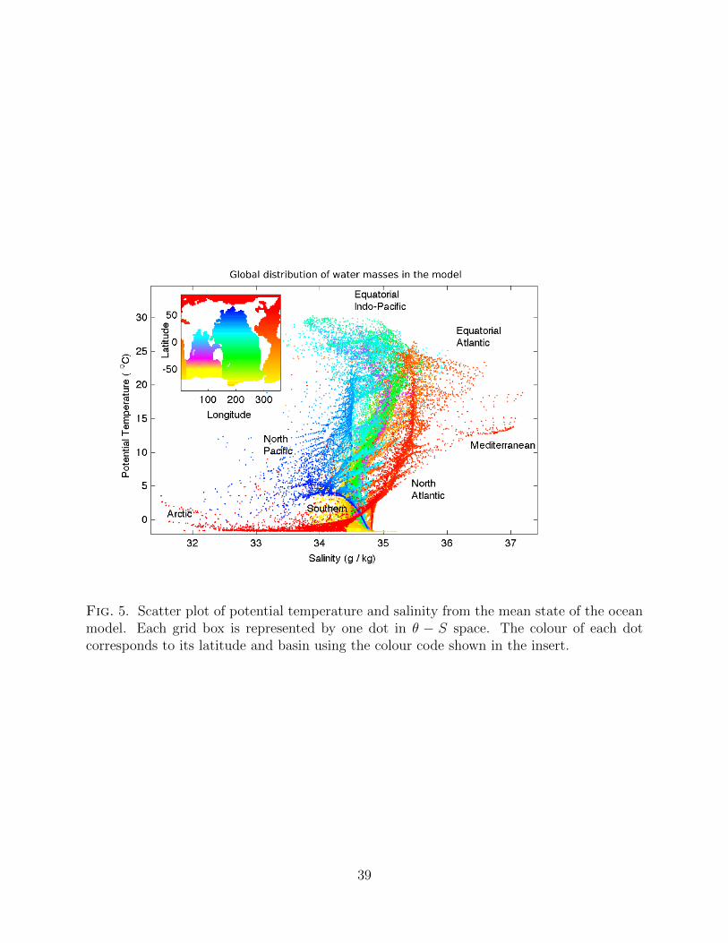
Fig. 5. Scatter plot of potential temperature and salinity from the mean state of the oceanmodel. Each grid box is represented by one dot in θ − S space. The colour of each dotcorresponds to its latitude and basin using the colour code shown in the insert.

39

252321191715131197531

135791113151719212325

Salinity (g/kg)

Pote

ntia

l Tem

pera

ture

(o C)

10 year mean Thermohaline Streamfunction (Sv)

33.5 34 34.5 35 35.5 36 36.5

0

5

10

15

20

25

30

Fig. 6. The thermohaline streamfunction derived from 10 years of monthly, u, v , w, θand S fields of the ocean model. Positive values are anti-clockwise and negative values areclockwise. The 4 Sv streamline is shown in red and the -4 Sv streamline in blue.

40

15

15

5

5

5

5

55

5

5 55

5

Pote

ntia

l Tem

pera

ture

(o C)

THS from u (!! S, Sv)

15

15

5

5

5

5

55

5

5 55

533.5 34 34.5 35 35.5 36 36.5

0

5

10

15

20

25

30

25

15

1515

5

55

5

5

5

5

5 5

5

THS from uEM (!EM

! S , Sv)

25

15

1515

5

55

5

5

5

5

5 5

533.5 34 34.5 35 35.5 36 36.5

0

5

10

15

20

25

30

5

5

5

Salinity (g / kg)

Pote

ntia

l Tem

pera

ture

(o C)

THS from uGM (!GM

!S , Sv)

5

5

5

33.5 34 34.5 35 35.5 36 36.5

0

5

10

15

20

25

30

39373533312927252321191715131197531

13579111315171921232527293133353739

5

55

5

5

5

55

Salinity (g / kg)

THS from u ! u (!!! S, Sv)

5

55

5

5

5

55

33.5 34 34.5 35 35.5 36 36.5

0

5

10

15

20

25

30

Fig. 7. Top left: THS from the sum of the time mean Euleran velocity and the time meaneddy-induced velocity (uEM + uGM). Top right: THS from the time mean Euleran velocity.Bottom left: THS from the time mean eddy-induced velocity. Bottom right: Differencebetween total THS and THS from the sum of the time mean Eulerian and eddy-inducedvelocities. That is, the contribution to the THS due to resolved fluctuations such as theseasonal cycle.

41

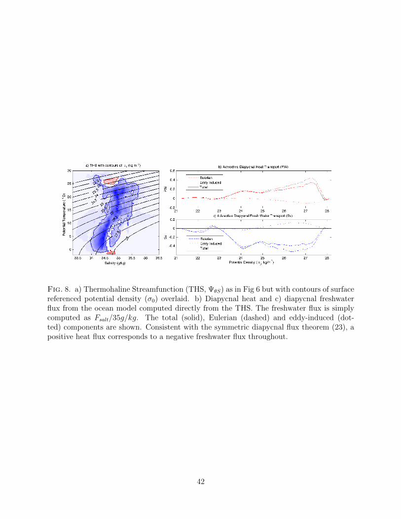
Fig. 8. a) Thermohaline Streamfunction (THS, ΨθS) as in Fig 6 but with contours of surfacereferenced potential density (σ0) overlaid. b) Diapycnal heat and c) diapycnal freshwaterflux from the ocean model computed directly from the THS. The freshwater flux is simplycomputed as Fsalt/35g/kg. The total (solid), Eulerian (dashed) and eddy-induced (dot-ted) components are shown. Consistent with the symmetric diapycnal flux theorem (23), apositive heat flux corresponds to a negative freshwater flux throughout.

42

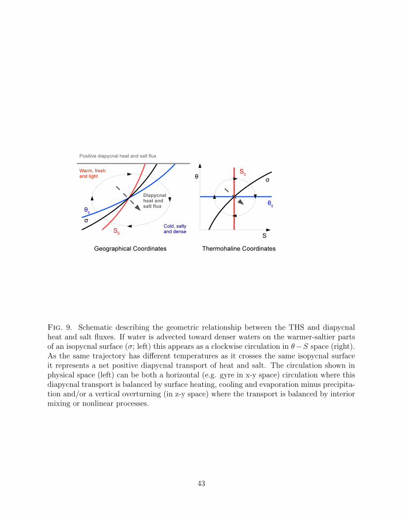
Fig. 9. Schematic describing the geometric relationship between the THS and diapycnalheat and salt fluxes. If water is advected toward denser waters on the warmer-saltier partsof an isopycnal surface (σ; left) this appears as a clockwise circulation in θ−S space (right).As the same trajectory has different temperatures as it crosses the same isopycnal surfaceit represents a net positive diapycnal transport of heat and salt. The circulation shown inphysical space (left) can be both a horizontal (e.g. gyre in x-y space) circulation where thisdiapycnal transport is balanced by surface heating, cooling and evaporation minus precipita-tion and/or a vertical overturning (in z-y space) where the transport is balanced by interiormixing or nonlinear processes.

43

33.5 34 34.5 35 35.5 365

0

5

10

15

20

25

30 Cumulative Thermohaline Transit Time (years)

Salinity (g/kg)

Pote

ntia

l Tem

pera

ture

(o C)

200

400

600

800

1000

1200

Fig. 10. The accumulated thermohaline transit of the -4Sv streamline. The colour ofeach dot represents the relative time taken along the streamline estimated using only thethermohaline streamfunction itself and the mean θ − S gradients.

44

25 20 15 10 5 0 5 10 15 200

500

1000

1500Thermohal ine Transi t Time (T! S)

Thermohaline Streamline (Sv)

Year

s

Global CellBottom Water Cell

0 5 10 15 200

10

20

30

Thermohaline Streamline (Sv)Ye

ars

Tropical Cell

Fig. 11. The thermohaline transit time of the longest THS streamlines in θ − S space (i.ethe longest streamlines in Fig. 6 for each transport). Shown are transit times for the globalcell (green), the bottom water cell (temperatures below 10oC), and the tropical cell contours(longest positive streamlines with temperatures above 10oC). The Antarctic Bottom Watertransit times may be underestimated due to interpolation onto a coarse θ − S grid.

45

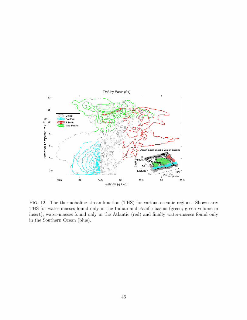
Fig. 12. The thermohaline streamfunction (THS) for various oceanic regions. Shown are:THS for water-masses found only in the Indian and Pacific basins (green; green volume ininsert), water-masses found only in the Atlantic (red) and finally water-masses found onlyin the Southern Ocean (blue).

46

Fig. 13. A thermohaline pathway projected into physical space. The -4 Sv THS contouris followed from the Atlantic water-masses (red in Fig. 12) to the Southern Ocean (blue inFig. 12) and then finally to the Indo-Pacific water-masses (bottom right panel). At pointsequally spaced in θ−S space along the contour, a colour is chosen to represent water-masseswith those water-mass properties (bottom right panel). All grid boxes in the correspondingregion with potential temperatures and salinities within 0.1◦C and 0.05 g / kg respectivelyof that point in θ − S space are then assigned the colour of that point. Top panel shows allgrid boxes above 300m. Middle panel: all grid boxes below 300m. Bottom left panel: onlyAltantic grid boxes. Bottom middle panel: Indo-Pacifc grid boxes.

47