'&

$%

Part (C): The Normal Distribution and Data Summaries

10 The Normal (Gaussian) distribution

(Reading: ‘Chance Encounters’, Seber & Wild, 6.1 - 6.3)

Some historical notes:

The normal curve was developed mathematically in 1733 by DeMoivre as an

approximation to the binomial distribution. His paper was not discovered until 1924

by Karl Pearson. Laplace used the normal curve in 1783 to describe the

distribution of errors. Subsequently, Gauss used the normal curve to analyze

astronomical data in 1809.

95

'&

$%

The normal distribution is the most used statistical distribution. The principal

reasons are:

1. Normally distributed random variables arise naturally in the context of

measurements such as height, weight, blood pressure, etc ...

2. Normality is important in statistical inference.

Often, if we take such a measurement over a large group of subjects, the resulting

histogram has a characteristic shape.

Example :

In 1836, the chest girths of 1516 US soldiers were measured. The distribution of

the measurements is shown in the following histogram.

96

'&

$%

Note:

(i) the symmetry of the histogram about the central value (35”)

(ii) the ‘bell’ shape of the observed distribution.

If we choose a soldier at random from the 1516 they are just as likely to have chest

girth > 3500 as < 3500. [due to (i)]

It is very unlikely to be > 4000 or < 3000. [due to (ii)]

The Normal distribution is often used to represent distributions such as the above.

97

'&

$%

10.1 Probability density function of the Normal distribution

If X is a normal random variable, its p.d.f. is given by

fX(x) =

1p2��e�

12�2(x��)2; �1 < x <1 (20)

�1 < � <1; � > 0:

The p.d.f. depends on the two basic parameters of the distribution, the meanE(X) = �

and the variance

var(X) = �2:

98

'&

$%

For a normal r.v. with mean � and variance �2 we use the notation

X � N(�; �2)

If we superimpose the graph of the normal p.d.f. with � = 35; �2 = 4 on the

chest-girth histogram we obtain a good fit. The density looks like a ‘smoother’

version of the histogram.

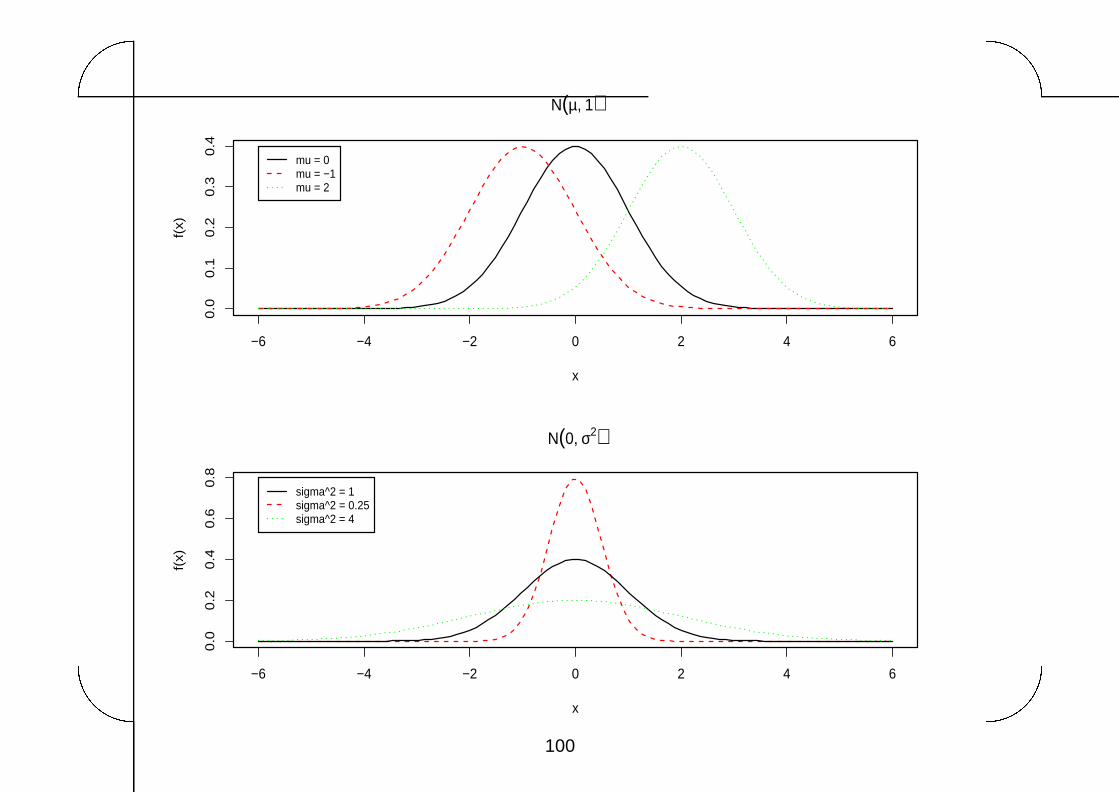
10.2 Important properties

1. The shape of the distribution

All normal densities have a ‘bell-shaped’ graph. They differ only in location (�) and

spread (�).

The graph of the N(�; �2) density is symmetric about the mean �.

If � is large the distribution (‘bell-shape’) will be wide.

If � is small the distribution will be narrow.

99

'&

$%

−6 −4 −2 0 2 4 6

0.0

0.1

0.2

0.3

0.4

x

f(x)

N(µ, 1)

mu = 0mu = −1mu = 2

−6 −4 −2 0 2 4 6

0.0

0.2

0.4

0.6

0.8

x

f(x)

N(0, σ2)

sigma^2 = 1sigma^2 = 0.25sigma^2 = 4

100

'&

$%

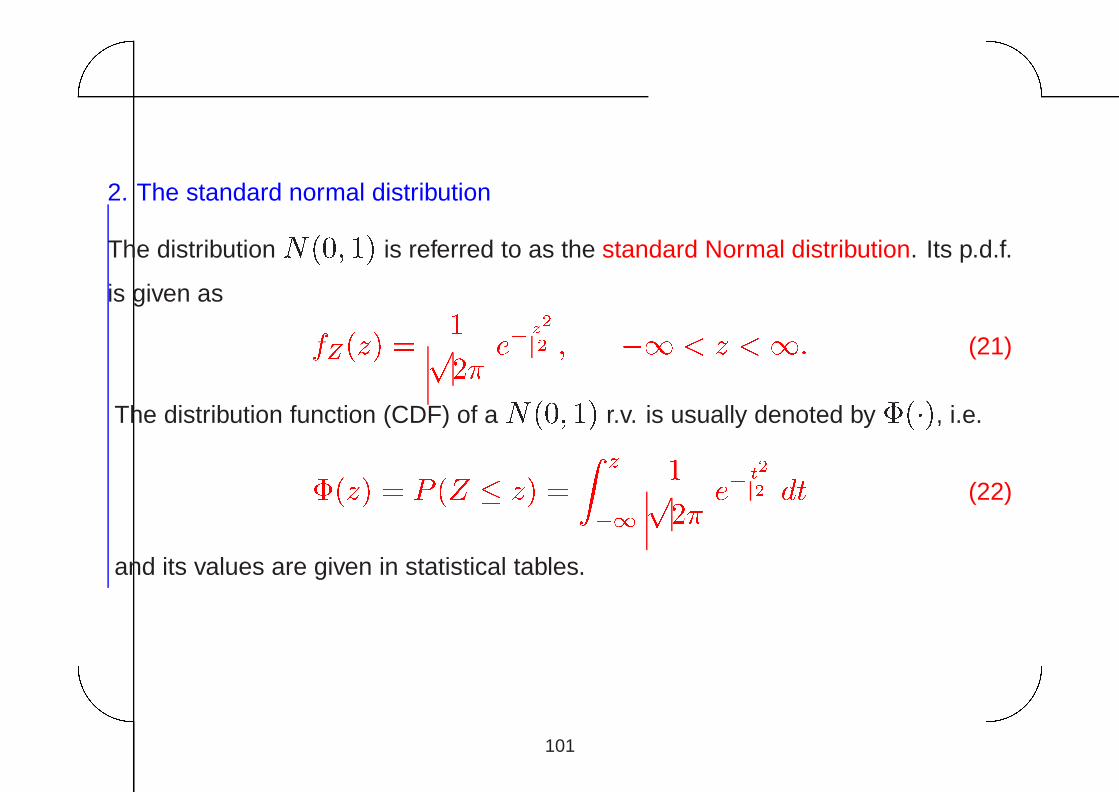
2. The standard normal distribution

The distribution N(0; 1) is referred to as the standard Normal distribution. Its p.d.f.

is given asfZ(z) =

1p2�e�

z

22 ; �1 < z <1: (21)

The distribution function (CDF) of a N(0; 1) r.v. is usually denoted by �(�), i.e.

�(z) = P (Z � z) =Z z

�1

1p2�e�

t2

2 dt (22)

and its values are given in statistical tables.

101

'&

$%

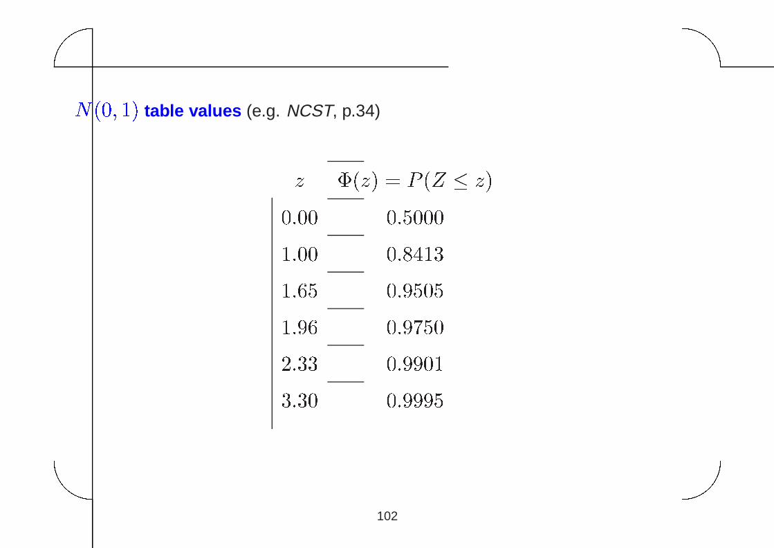
N(0; 1) table values (e.g. NCST, p.34)

z �(z) = P (Z � z)

0:00 0:5000

1:00 0:8413

1:65 0:9505

1:96 0:9750

2:33 0:9901

3:30 0:9995

102

'&

$%

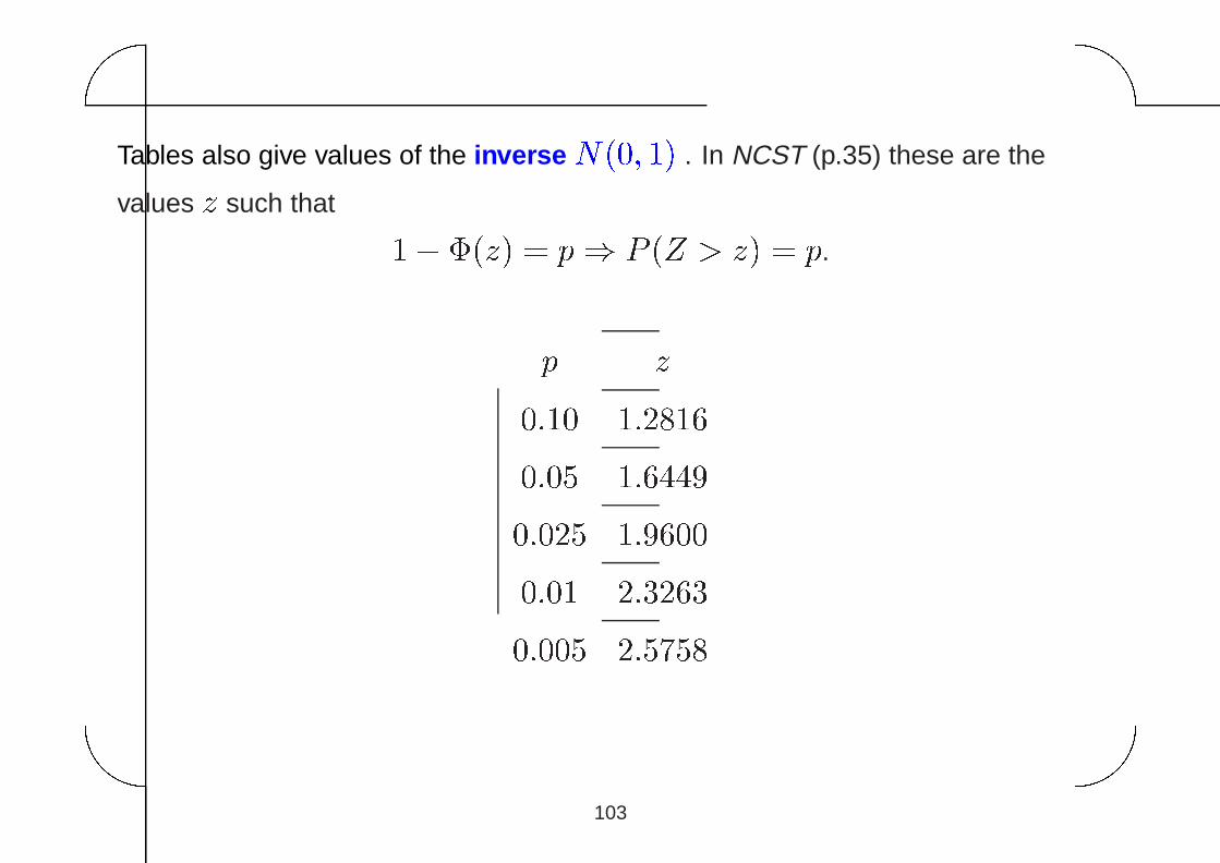
Tables also give values of the inverse N(0; 1) . In NCST (p.35) these are the

values z such that

1� �(z) = p) P (Z > z) = p.

p z

0:10 1:2816

0:05 1:6449

0:025 1:9600

0:01 2:3263

0:005 2:5758

103

'&

$%

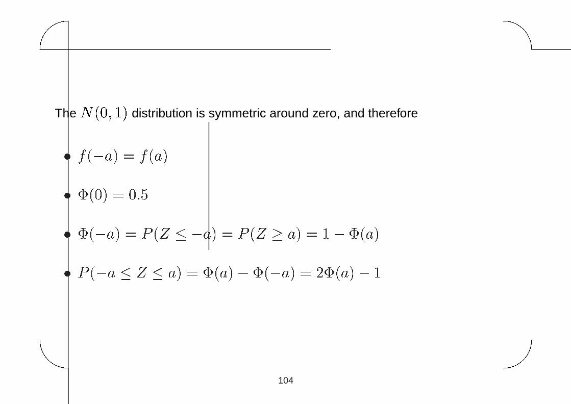
The N(0; 1) distribution is symmetric around zero, and therefore

� f(�a) = f(a)

� �(0) = 0:5

� �(�a) = P (Z � �a) = P (Z � a) = 1� �(a)

� P (�a � Z � a) = �(a)� �(�a) = 2�(a)� 1104

'&

$%

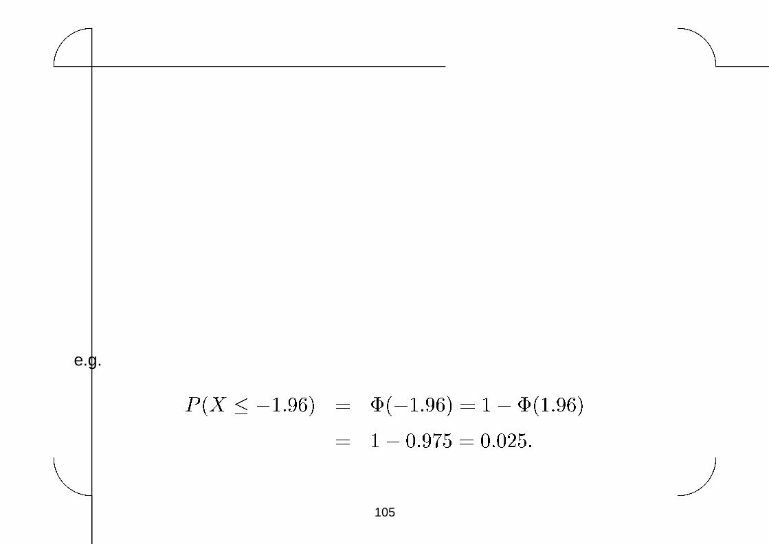
e.g.

P (X � �1:96) = �(�1:96) = 1� �(1:96)

= 1� 0:975 = 0:025:105

'&

$%

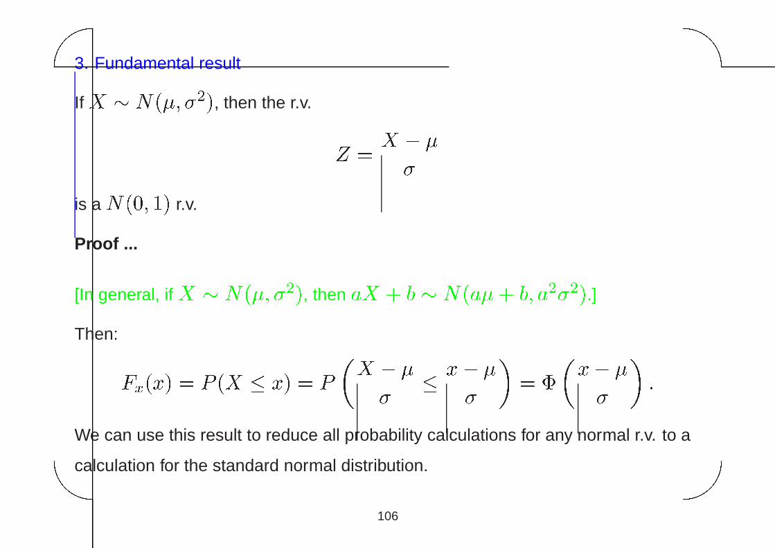
3. Fundamental result

If X � N(�; �2), then the r.v.

Z =

X � ��

is a N(0; 1) r.v.

Proof ...

[In general, if X � N(�; �2), then aX + b � N(a�+ b; a2�2).]

Then:

Fx(x) = P (X � x) = P�

X � ��

� x� ��

�= �

�x� �

�

�:

We can use this result to reduce all probability calculations for any normal r.v. to a

calculation for the standard normal distribution.

106

'&

$%

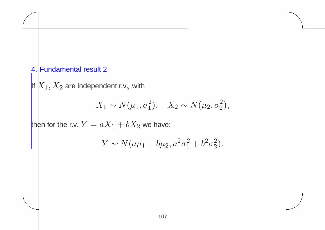
4. Fundamental result 2

If X1;X2 are independent r.vs withX1 � N(�1; �2

1); X2 � N(�2; �2

2);

then for the r.v. Y = aX1 + bX2 we have:

Y � N(a�1 + b�2; a2�21 + b2�22):

107

'&

$%

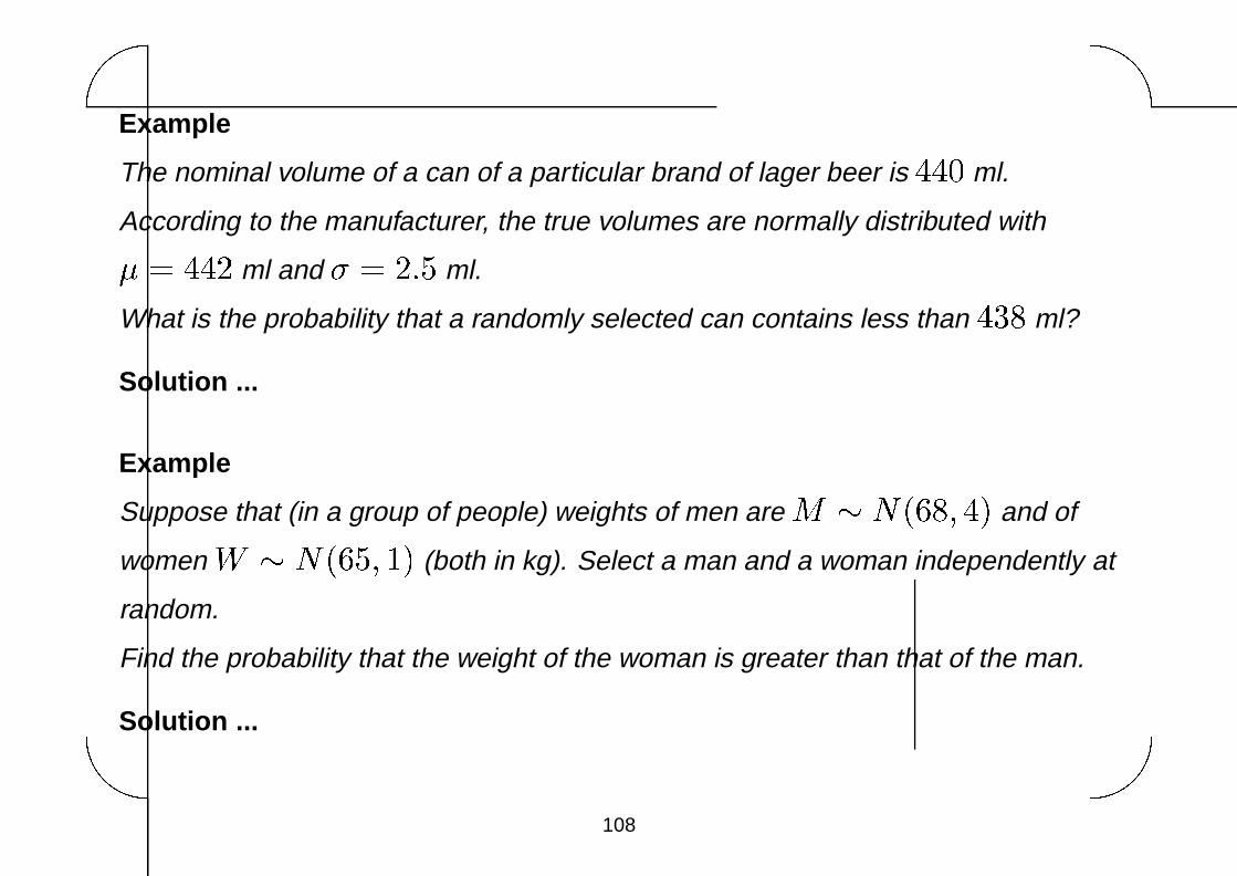
Example

The nominal volume of a can of a particular brand of lager beer is 440 ml.

According to the manufacturer, the true volumes are normally distributed with

� = 442 ml and � = 2:5 ml.

What is the probability that a randomly selected can contains less than 438 ml?

Solution ...

Example

Suppose that (in a group of people) weights of men are M � N(68; 4) and of

women W � N(65; 1) (both in kg). Select a man and a woman independently at

random.

Find the probability that the weight of the woman is greater than that of the man.

Solution ...

108

'&

$%

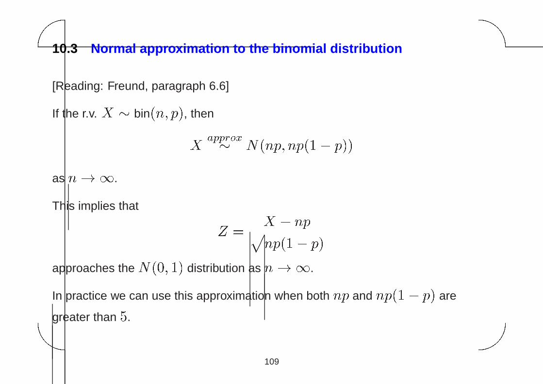
10.3 Normal approximation to the binomial distribution

[Reading: Freund, paragraph 6.6]

If the r.v. X � bin(n; p), then

X

approx� N(np; np(1� p))

as n!1.

This implies thatZ =

X � nppnp(1� p)

approaches the N(0; 1) distribution as n!1.

In practice we can use this approximation when both np and np(1� p) are

greater than 5.

109

'&

$%

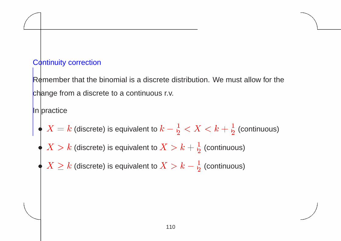
Continuity correction

Remember that the binomial is a discrete distribution. We must allow for the

change from a discrete to a continuous r.v.

In practice

� X = k (discrete) is equivalent to k � 12< X < k + 12

(continuous)

� X > k (discrete) is equivalent to X > k + 12

(continuous)

� X � k (discrete) is equivalent to X > k � 12

(continuous)

110

'&

$%

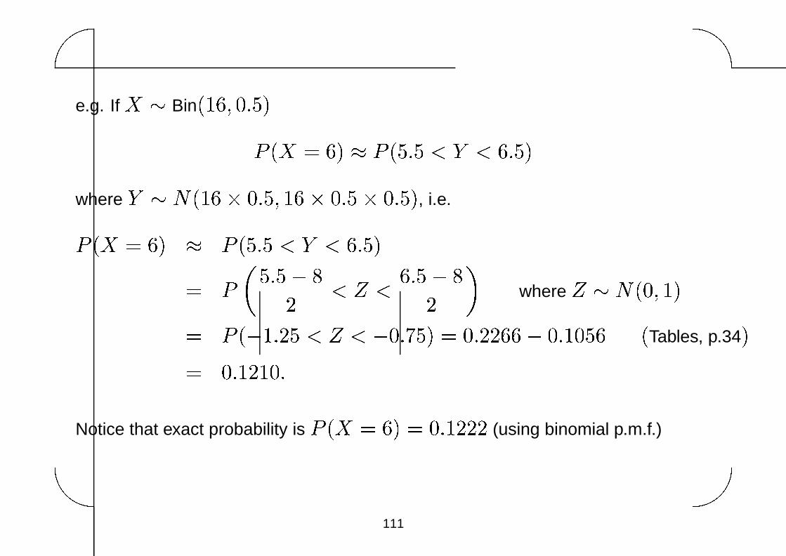
e.g. If X � Bin(16; 0:5)P (X = 6) � P (5:5 < Y < 6:5)

where Y � N(16� 0:5; 16� 0:5� 0:5), i.e.

P (X = 6) � P (5:5 < Y < 6:5)

= P�

5:5� 8

2

< Z <

6:5� 8

2

�

where Z � N(0; 1)

= P (�1:25 < Z < �0:75) = 0:2266� 0:1056 (Tables, p.34)

= 0:1210:

Notice that exact probability is P (X = 6) = 0:1222 (using binomial p.m.f.)

111

'&

$%

Descriptive statistics� Organisation and presentation of data

– tables, frequency distributions

– visual displays: bar charts, histograms, stem-and-leaf plots etc.

� Summary of data

– measures of location: median, mean, mode etc.

– measures of spread: range, standard deviation etc.

– description of shape: e.g. skewness

– outliers (extreme values), transformations

� Overall summaries

– e.g. 5-point summaries, boxplots

112

'&

$%

11 Summarising continuous data: Graphical summaries

This should be the first step to a good statistical analysis.

Graphical summaries help identify the main characteristics of the data, e.g.

whether our data look consistent with a Normal distribution.

All graphs should:

� be reasonably accurate

� be on the correct (appropriate) scale

� have good annotation (title,labels on axes, units etc.)

113

'&

$%

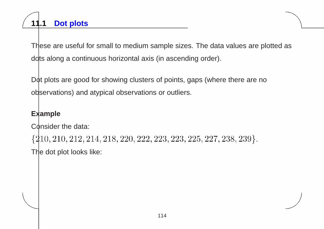
11.1 Dot plots

These are useful for small to medium sample sizes. The data values are plotted as

dots along a continuous horizontal axis (in ascending order).

Dot plots are good for showing clusters of points, gaps (where there are no

observations) and atypical observations or outliers.

Example

Consider the data:

f210; 210; 212; 214; 218; 220; 222; 223; 223; 225; 227; 238; 239g.

The dot plot looks like:

114

'&

$%

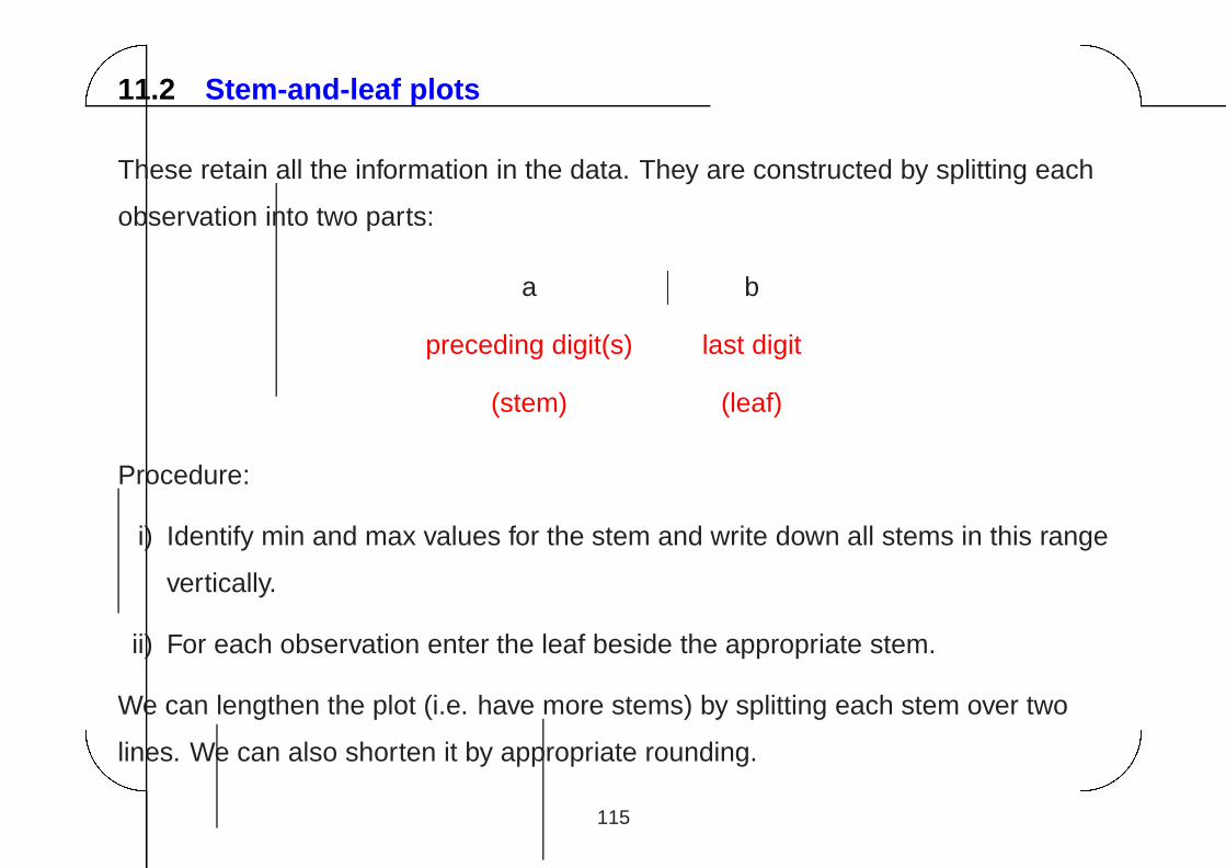
11.2 Stem-and-leaf plots

These retain all the information in the data. They are constructed by splitting each

observation into two parts:

a j b

preceding digit(s) last digit

(stem) (leaf)

Procedure:

i) Identify min and max values for the stem and write down all stems in this range

vertically.

ii) For each observation enter the leaf beside the appropriate stem.

We can lengthen the plot (i.e. have more stems) by splitting each stem over two

lines. We can also shorten it by appropriate rounding.

115

'&

$%

Example

Consider the data from previous example:f210; 210; 212; 214; 218; 220; 222; 223; 223; 225; 227; 238; 239g.

The stem-and-leaf plot looks like:

116

'&

$%

11.3 Histograms

Also very useful for representing continuous data graphically.

To form a histogram from the observations x1; x2; : : : ; xn we simply:

i) Identify min and max observations.

ii) Split the range of the values into equal intervals (bins) (e.g. between 5 and 15

bins).

iii) Count the observations falling in each bin.

iv) Draw a rectangle above each interval with height equal to the number of

observations in that interval.

117

'&

$%

Notice that:� Alternatively we can draw rectangles with height equal to the proportion of

observations falling in each bin.

� The intervals (in step ii. above) can have unequal length (perhaps at the

extremes of the distribution).

In that case the area of the rectangles (not their height) should be equal (or

proportional) to the bin frequencies.

Histograms and stem-and-leaf plots are very useful for checking whether the data

look Normal.

Remember that if this is the case the histogram should look (roughly)

� symmetric

� ‘bell-shaped’

118

'&

$%

Watch out for obvious deviations from this pattern, e.g.� More than one mode (peak)

This pattern can occur when a measurement is taken on a population

consisting of two distinct sub-populations (e.g. males - females)

� Lack of symmetry (skewness)

119

'&

$%

12 Summarising continuous data: Numerical summaries

Numerical summaries provide useful and informative measures of the main

features of the data.

12.1 Measures of location

1. The sample mean

If x1; x2; : : : ; xn constitute a random sample, then the sample mean is given by�x =

1n

nXi=1

xi

120

'&

$%

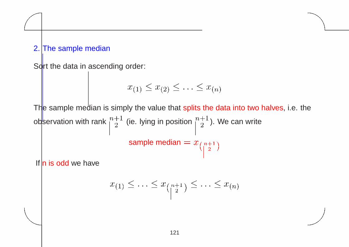
2. The sample median

Sort the data in ascending order:

x(1) � x(2) � : : : � x(n)

The sample median is simply the value that splits the data into two halves, i.e. the

observation with rank n+12

(ie. lying in position n+12

). We can write

sample median = x(n+1

2 )

If n is odd we have

x(1) � : : : � x(n+1

2 )� : : : � x(n)

121

'&

$%

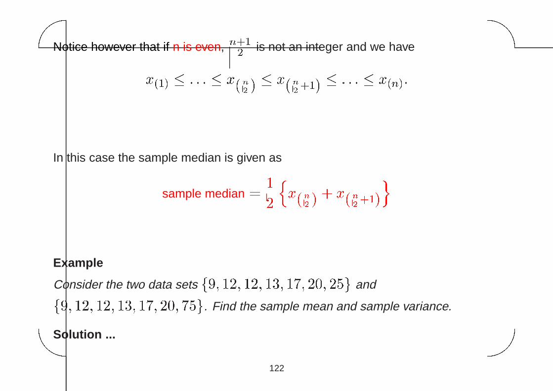
Notice however that if n is even, n+12

is not an integer and we have

x(1) � : : : � x(n

2 )� x(n

2+1)� : : : � x(n):

In this case the sample median is given as

sample median =1

2n

x(n

2 )+ x(n

2+1)o

Example

Consider the two data sets f9; 12; 12; 13; 17; 20; 25g and

f9; 12; 12; 13; 17; 20; 75g. Find the sample mean and sample variance.

Solution ...

122

'&

$%

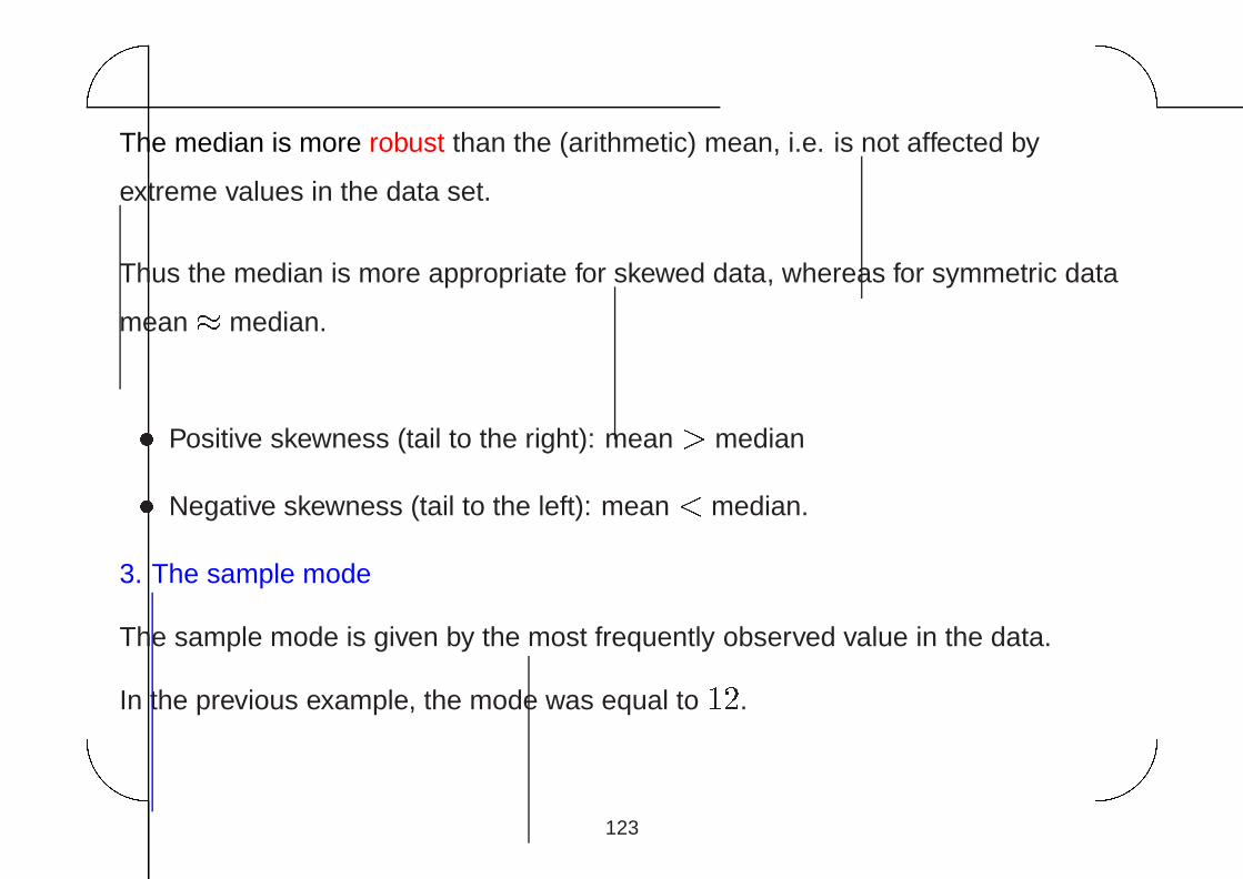
The median is more robust than the (arithmetic) mean, i.e. is not affected by

extreme values in the data set.

Thus the median is more appropriate for skewed data, whereas for symmetric data

mean� median.

� Positive skewness (tail to the right): mean > median

� Negative skewness (tail to the left): mean < median.

3. The sample mode

The sample mode is given by the most frequently observed value in the data.

In the previous example, the mode was equal to 12.

123

'&

$%

12.2 Measures of spread (dispersion, variation)

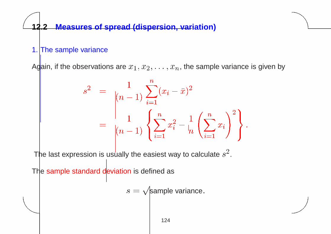
1. The sample variance

Again, if the observations are x1; x2; : : : ; xn, the sample variance is given by

s2 =

1

(n� 1)

nXi=1

(xi � �x)2

=

1

(n� 1)8<

:nX

i=1x2i �1

n

nXi=1xi

!29=

; :

The last expression is usually the easiest way to calculate s2.

The sample standard deviation is defined as

s =p

sample variance:

124

'&

$%

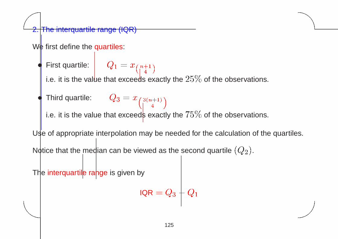
2. The interquartile range (IQR)

We first define the quartiles:

� First quartile: Q1 = x(n+1

4 )

i.e. it is the value that exceeds exactly the 25% of the observations.

� Third quartile: Q3 = x� 3(n+1)

4

�

i.e. it is the value that exceeds exactly the 75% of the observations.

Use of appropriate interpolation may be needed for the calculation of the quartiles.

Notice that the median can be viewed as the second quartile (Q2).

The interquartile range is given by

IQR = Q3 �Q1

125

'&

$%

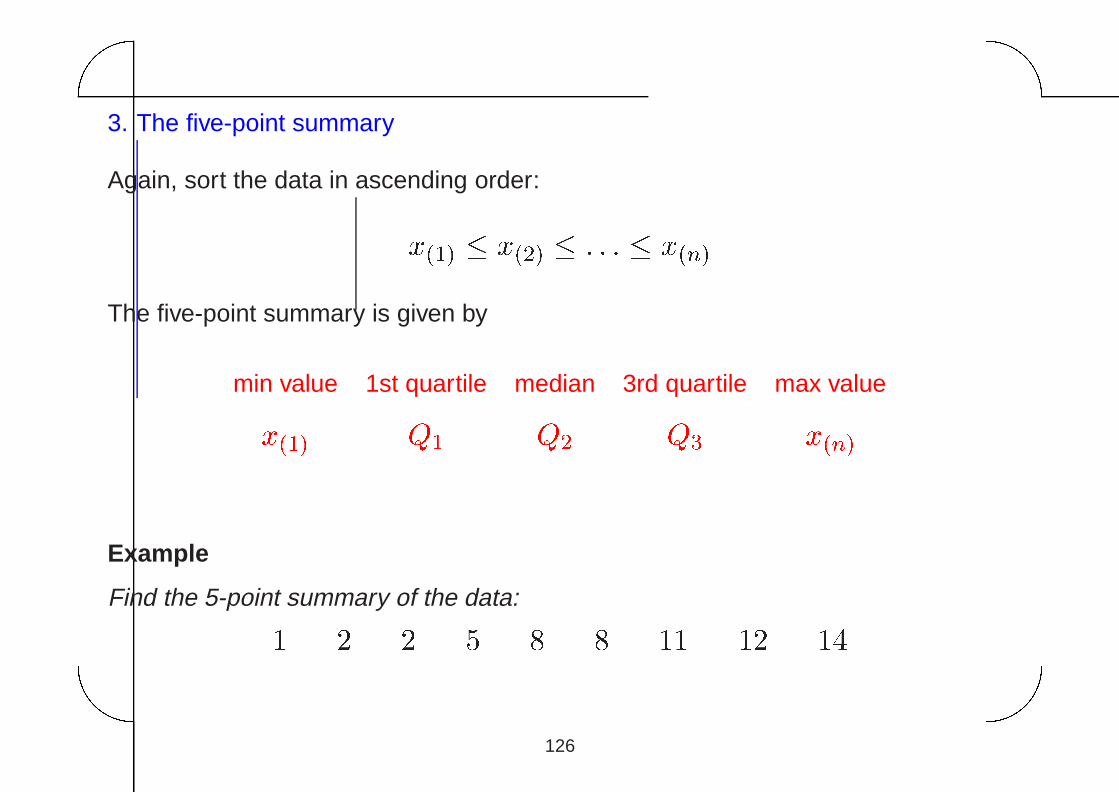
3. The five-point summary

Again, sort the data in ascending order:

x(1) � x(2) � : : : � x(n)

The five-point summary is given by

min value 1st quartile median 3rd quartile max value

x(1) Q1 Q2 Q3 x(n)

Example

Find the 5-point summary of the data:

1 2 2 5 8 8 11 12 14

126

'&

$%

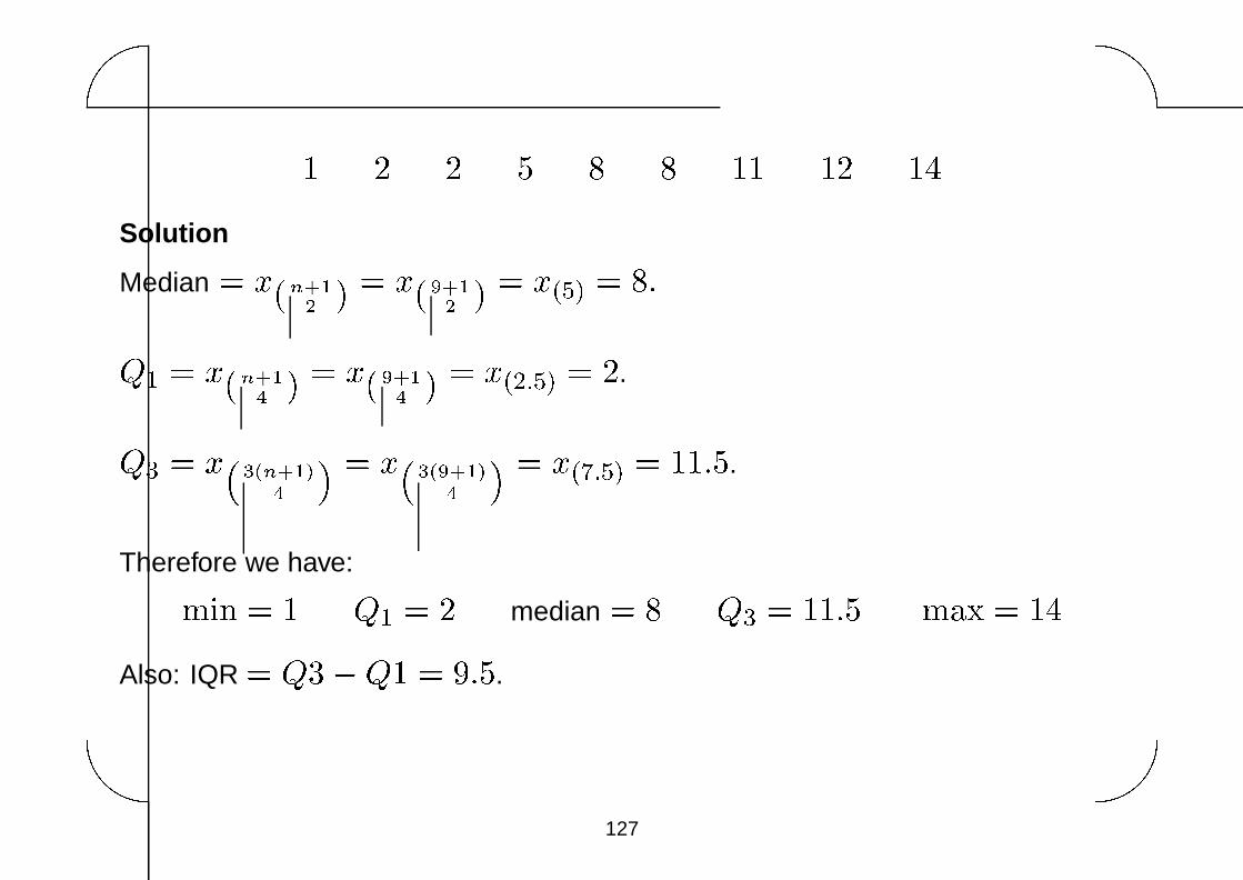
1 2 2 5 8 8 11 12 14

Solution

Median = x(n+1

2 )= x(9+1

2 )= x(5) = 8:

Q1 = x(n+1

4 )= x(9+1

4 )= x(2:5) = 2.

Q3 = x� 3(n+1)

4

� = x� 3(9+1)

4

� = x(7:5) = 11:5.

Therefore we have:

min = 1 Q1 = 2 median = 8 Q3 = 11:5 max = 14

Also: IQR = Q3�Q1 = 9:5.

127

'&

$%

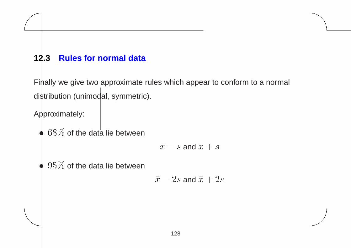
12.3 Rules for normal data

Finally we give two approximate rules which appear to conform to a normal

distribution (unimodal, symmetric).

Approximately:

� 68% of the data lie between

�x� s and �x+ s

� 95% of the data lie between

�x� 2s and �x+ 2s

128