The Nonlinear Dynamical and Shock Mitigation …Army Research Laboratory Aberdeen Proving Ground, MD 21005 ARL-RP-0211 June 2008 The Nonlinear Dynamical and Shock Mitigation Properties

The Nonlinear Dynamical and Shock Mitigation Properties

of Tapered Chains

by Robert Doney

ARL-RP-0211 June 2008 Approved for public release; distribution unlimited.

NOTICES

Disclaimers The findings in this report are not to be construed as an official Department of the Army position unless so designated by other authorized documents. Citation of manufacturer’s or trade names does not constitute an official endorsement or approval of the use thereof. Destroy this report when it is no longer needed. Do not return it to the originator.

Army Research Laboratory Aberdeen Proving Ground, MD 21005

ARL-RP-0211 June 2008 The Nonlinear Dynamical and Shock Mitigation Properties

of Tapered Chains

Robert Doney Weapons & Materials Research Directorate, ARL

Approved for public release; distribution unlimited.

ii

REPORT DOCUMENTATION PAGE Form Approved OMB No. 0704-0188

Public reporting burden for this collection of information is estimated to average 1 hour per response, including the time for reviewing instructions, searching existing data sources, gathering and maintaining the data needed, and completing and reviewing the collection information. Send comments regarding this burden estimate or any other aspect of this collection of information, including suggestions for reducing the burden, to Department of Defense, Washington Headquarters Services, Directorate for Information Operations and Reports (0704-0188), 1215 Jefferson Davis Highway, Suite 1204, Arlington, VA 22202-4302. Respondents should be aware that notwithstanding any other provision of law, no person shall be subject to any penalty for failing to comply with a collection of information if it does not display a currently valid OMB control number. PLEASE DO NOT RETURN YOUR FORM TO THE ABOVE ADDRESS.

1. REPORT DATE (DD-MM-YYYY)

June 2008 2. REPORT TYPE

Progress 3. DATES COVERED (From - To)

January 2004 to January 2007 5a. CONTRACT NUMBER

5b. GRANT NUMBER

4. TITLE AND SUBTITLE

The Nonlinear Dynamical and Shock Mitigation Properties of Tapered Chains

5c. PROGRAM ELEMENT NUMBER

5d. PROJECT NUMBER

5e. TASK NUMBER

6. AUTHOR(S)

Robert Doney

5f. WORK UNIT NUMBER

7. PERFORMING ORGANIZATION NAME(S) AND ADDRESS(ES)

U.S. Army Research Laboratory ATTN: AMSRD-ARL-WM-TA Weapons & Materials Research Directorate Aberdeen Proving Ground, MD 21005

8. PERFORMING ORGANIZATION REPORT NUMBER ARL-RP-0211

10. SPONSOR/MONITOR'S ACRONYM(S)

9. SPONSORING/MONITORING AGENCY NAME(S) AND ADDRESS(ES)

11. SPONSOR/MONITOR'S REPORT NUMBER(S)

12. DISTRIBUTION/AVAILABILITY STATEMENT

Approved for public release; distribution unlimited. 13. SUPPLEMENTARY NOTES 14. ABSTRACT

An analytic and numerical study of the problem of mechanical impulse propagation through a horizontal alignment of progressively shrinking (tapered) elastic spheres that are placed between two rigid end walls is investigated. Particular attention is paid to the shock absorption and nonlinear dynamical properties as they pertain to energy partition. The studies are confined to cases where initial loading between the spheres is zero. The spheres are assumed to interact via the purely repulsive and strongly nonlinear Hertz potential. Propagation of energy is analytically studied in the hard-sphere approximation and parameter space diagrams plotting normalized kinetic energy of the smallest grain at the tapered end are developed for various chain lengths and tapering factors. These details are then compared to congruent diagrams obtained via extensive dynamical simulations. Our figures indicate that the ratios of the kinetic energies of the smallest to largest grains possess a gaussian dependence on tapering and an exponential decay when the number of grains increases. The results demonstrate the capability of these chains to thermalize propagating impulses and thereby act as potential shock absorbing devices.

15. SUBJECT TERMS

16. SECURITY CLASSIFICATION OF: 19a. NAME OF RESPONSIBLE PERSON Robert Doney

a. REPORT

U b. ABSTRACT

U c. THIS PAGE

U

17. LIMITATIONOF ABSTRACT

SAR

18. NUMBEROF PAGES

147 19b. TELEPHONE NUMBER (Include area code) 410-278-7309

Standard Form 298 (Rev. 8/98) Prescribed by ANSI Std. Z39.18

THE NONLINEAR DYNAMICAL AND SHOCK MITIGATIONPROPERTIES OF TAPERED CHAINS

BY

ROBERT L. DONEY III

B.S., George Mason University, 1995M.S., George Mason University, 2001

DISSERTATION

A Dissertation submitted to theFaculty of the Graduate School of

The State University of New York at Bu!aloin partial fulfillment of the requirements for the

degree of

( Doctor of Philosophy )

Department of Physics

For Joey

Joseph Randall Ray

Feb. 27, 1977 - March 12, 2006

Sta! Sgt., 391st Engineer Battalion, U.S. Army Reserve, Asheville, N.C

Last mission: Road clearing operations in Asadabad, Afghanistan

Son :: Brother :: Husband :: Father :: Friend :: Patriot

iii

Acknowledgements

I would like to first thank my advisor, Professor Sen, for introducing me to this intriguing and

relevant problem. He has been a great mentor and friend during the 3 years that I’ve known him

and allowed the flexibility I needed to complete this work in absentia from the University, carry on

with a full-time job, and be a father and husband. Secondly, Im indebted to my committee members,

Professors Bruce Pitman and Richard Gonsalves, for taking time out of their busy schedules to read

and evaluate the research in this dissertation and upcoming defense. Thanks so much to all of you.

I am lucky to be married to such a supportive and devoted wife and best-friend, Stacy, who

also happened to be the babe in my dreams. She has helped me maintain my sanity and focus on

countless occasions, even though I haven’t been able to reciprocate as often due to the commitments

this degree has required. This has gone on through the birth of our two wonderful girls, Sarah and

Cora. I am happy to say that I don’t have to hide in the basement in front of the computer most

every weekend anymore. I love them all and this work could not have been completed without their

strength.

I cannot thank enough my parents, Robert and Mattie, who have supported me in numerous

ways since I started college — just a few of which includes living at home while completing a B.S.

at GMU, financial support, encouragement, and rides back and forth to NVCC when I didn’t have

a car. There’s no way I could have gotten anywhere as far without their love and support. I’d

also like to thank my parents-in-law, Dave and Gina Moore, for their support since they’ve been

through this before. Thanks to my sister, Dawn and her family Brian, Katherine, and Christopher

for their encouragement and rocket scientist jokes. On the latter point, many thanks also to Randy,

Helen, Tyler, and Kimberly Ray for their kind words and hospitality. They know what all the fuss

is about. Thanks to Paw, Grandma (who passed away in my first year at SUNY) and my extended

family — Ruane, Ronda, Lisa, and Rita and their families for their support and love. I’d also like to

thank my posse from Fairfax who have watched all this work from the sidelines and rightfully shaken

their heads. Thanks for the kegs, the parties, the laughter, the movies, the memories, and the +5

iv

Hammer of Thunderbolts and Belt of Giant Strength being worn by a Kobald: Ryan, Leigh, Justin,

C.J., Alex, Dave, Koz, Jason, Matt, Shannon, Neil, Monte, Wojtek, Steve, Tom, Adair, Cindy, Sue,

Mike, and Heather.

This dissertation ends about 473 Megaseconds1 of time spent pursing degrees. During that

period I’ve accumulated that many years of “professional” work experience from a bookstore (where

I met Stacy!), the Radiation Research lab at Ft. Belvoir, NASA, Orbital Sciences, the Institute for

Defense Analyses (IDA), and currently, the U.S. Army Research Laboratory. I have been fortunate

to cross paths with many interesting people. Several of them have steered my career in some way

and I’d like to recognize them — hopefully in chronological order.

To Mr. Runzo at Fairfax High School for getting me really intrigued in Physics. The episodes

of the “Mechanical Universe” were a really cool way to go into the weekend.

Walerian Majewski, professor of Physics at Northern Virginia Community College was a big

force early in my career (fall 90-spring 92). A serious chalkboard jockey, he had boundless energy

in creating and getting us active in the Society of Physics Students. We gave presentations, did

research on the relativistic lifetime extension of cosmic ray muons, built superconducting Meissner

engines, collected data from the GEOS weather satellite, and did public outreach to local schools.

Later I took a course from him in electromagnetics at GMU (fall 93) and his recommendation got

me out of making $5.70 per hour at Supercrown books and into the Radiation Research Lab making

$10.00 per hour. Sweet.

To Ram Bhat, Tim Mikulski, Tom Brown, and Walter Klaus for making work at the Radiation

lab fun and safe. Well almost safe. I did safety surveys of an X-ray machine that must have been

the original prototype. The safety interlock didn’t work on the sampler input and the meter kept

going o! scale on my Geiger counter as I turned up the scale by 10x several times. A urine analysis

later revealed it was just a few chest X-rays worth of dosage — at least they were free. And here’s

to the unsanctioned liquid nitrogen experiments. There’s nothing quite like the yelp from someone

who has had a super-cooled eraser placed on their bald head. How fast does a spider shrivel up

when placed in liquid NO2? Fast. And in regard to the infamous all-you-can-eat student farewell

party, no one...no one I say can eat 14 slices of meat and cheese lover’s pan pizza for lunch and keep

it down.

Thanks are extended to Pepsi for inventing Mountain Dew which kept me wired and vibrating for

hours into the night. Twenty pounds later, I had to switch to Diet Mountain Dew: all the ca!eine

without the calories, who knew?115 years. For a good laugh, check out http://en.wikipedia.org/wiki/Attoparsec

v

I’m indebted to the many talented people at IDA and the role they played in getting me to where

I am today. Gordie Boezer was an outstanding mentor and taught me quite a bit about diplomacy.

Norm Jorstad, Mike Rigdon, and John Frasier also were invaluable in my professional development.

Ira Kohlberg taught me that there is always more to teach somebody about computers. And Jim

Heagy taught me there was someone who loathed microsoft’s bloatware products more than myself.

It was at IDA that I met Jim Sarjeant who invited me to SUNY Bu!alo to work on microdischarge

in insulators. Thanks go to him for introducing me to Bill Bruchey. I’d also like to thank Doug

Hopkins, Harry Gill and Erik Altho! for making the EE experience fun. After a year and loss of

interest there however, I decided to come back to physics where I found new challenges awaiting

me in such treasures as Baym (in particular problem 11.2), Jackson, and Ashcroft and Mermin. I

was lucky to become friends with several people and enjoyed their company around the BBQ grill.

Many thanks go to Joe Helfer and Brian Powell for the awesome racquetball games. It’s great to

see them struggle so much when we play — after all, what dissertation is complete without a little

smack-talk? I’d also like to thank Bill Condit who introduced me to Professor Sen as well as Marlene

Kowalski, Pat Meider, and Joe Helfer for administrative support throughout the years.

Finally, I’m greatly indebted to ARL and the many people there who have fully supported all

my academic ventures. In particular, thanks go to Bill Bruchey for bringing me in and getting me

hired as a government employee; Mike Zoltoski for helping me get reimbursed, and Mike Keele for

mentoring me. Scott Schoenfeld and John Runyeon have both strongly supported my education

and required travel to Bu!alo and APS-sponsored conferences to present the research. Finally, I’m

indebted to John Powell, Chuck Hummer and Carl Krauthauser for their interest and review of this

work for various publications.

vi

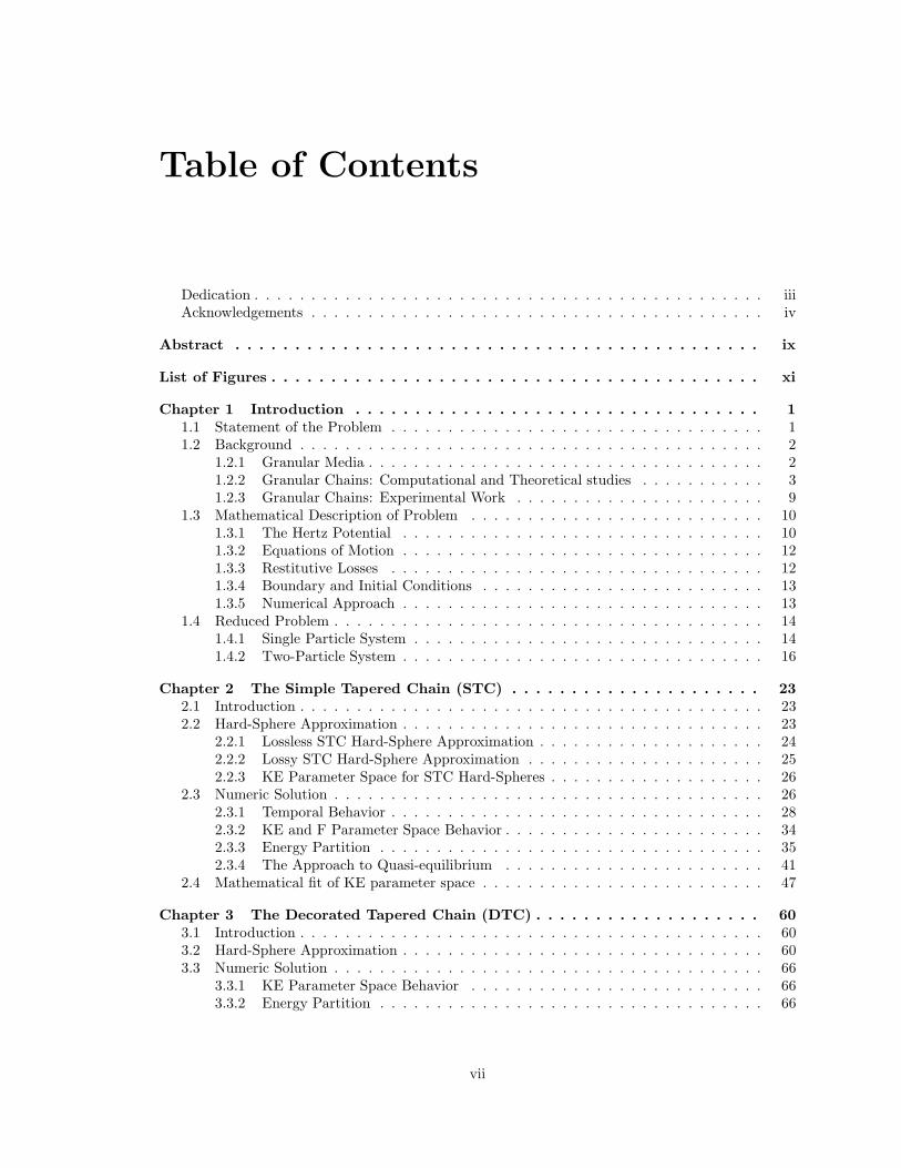
Table of Contents

Dedication . . . . . . . . . . . . . . . . . . . . . . . . . . . . . . . . . . . . . . . . . . . . . iiiAcknowledgements . . . . . . . . . . . . . . . . . . . . . . . . . . . . . . . . . . . . . . . . iv

Abstract . . . . . . . . . . . . . . . . . . . . . . . . . . . . . . . . . . . . . . . . . . . . ix

List of Figures . . . . . . . . . . . . . . . . . . . . . . . . . . . . . . . . . . . . . . . . . xi

Chapter 1 Introduction . . . . . . . . . . . . . . . . . . . . . . . . . . . . . . . . . . 11.1 Statement of the Problem . . . . . . . . . . . . . . . . . . . . . . . . . . . . . . . . . 11.2 Background . . . . . . . . . . . . . . . . . . . . . . . . . . . . . . . . . . . . . . . . . 2

1.2.1 Granular Media . . . . . . . . . . . . . . . . . . . . . . . . . . . . . . . . . . . 21.2.2 Granular Chains: Computational and Theoretical studies . . . . . . . . . . . 31.2.3 Granular Chains: Experimental Work . . . . . . . . . . . . . . . . . . . . . . 9

1.3 Mathematical Description of Problem . . . . . . . . . . . . . . . . . . . . . . . . . . 101.3.1 The Hertz Potential . . . . . . . . . . . . . . . . . . . . . . . . . . . . . . . . 101.3.2 Equations of Motion . . . . . . . . . . . . . . . . . . . . . . . . . . . . . . . . 121.3.3 Restitutive Losses . . . . . . . . . . . . . . . . . . . . . . . . . . . . . . . . . 121.3.4 Boundary and Initial Conditions . . . . . . . . . . . . . . . . . . . . . . . . . 131.3.5 Numerical Approach . . . . . . . . . . . . . . . . . . . . . . . . . . . . . . . . 13

1.4 Reduced Problem . . . . . . . . . . . . . . . . . . . . . . . . . . . . . . . . . . . . . . 141.4.1 Single Particle System . . . . . . . . . . . . . . . . . . . . . . . . . . . . . . . 141.4.2 Two-Particle System . . . . . . . . . . . . . . . . . . . . . . . . . . . . . . . . 16

Chapter 2 The Simple Tapered Chain (STC) . . . . . . . . . . . . . . . . . . . . . 232.1 Introduction . . . . . . . . . . . . . . . . . . . . . . . . . . . . . . . . . . . . . . . . . 232.2 Hard-Sphere Approximation . . . . . . . . . . . . . . . . . . . . . . . . . . . . . . . . 23

2.2.1 Lossless STC Hard-Sphere Approximation . . . . . . . . . . . . . . . . . . . . 242.2.2 Lossy STC Hard-Sphere Approximation . . . . . . . . . . . . . . . . . . . . . 252.2.3 KE Parameter Space for STC Hard-Spheres . . . . . . . . . . . . . . . . . . . 26

2.3 Numeric Solution . . . . . . . . . . . . . . . . . . . . . . . . . . . . . . . . . . . . . . 262.3.1 Temporal Behavior . . . . . . . . . . . . . . . . . . . . . . . . . . . . . . . . . 282.3.2 KE and F Parameter Space Behavior . . . . . . . . . . . . . . . . . . . . . . . 342.3.3 Energy Partition . . . . . . . . . . . . . . . . . . . . . . . . . . . . . . . . . . 352.3.4 The Approach to Quasi-equilibrium . . . . . . . . . . . . . . . . . . . . . . . 41

2.4 Mathematical fit of KE parameter space . . . . . . . . . . . . . . . . . . . . . . . . . 47

Chapter 3 The Decorated Tapered Chain (DTC) . . . . . . . . . . . . . . . . . . . 603.1 Introduction . . . . . . . . . . . . . . . . . . . . . . . . . . . . . . . . . . . . . . . . . 603.2 Hard-Sphere Approximation . . . . . . . . . . . . . . . . . . . . . . . . . . . . . . . . 603.3 Numeric Solution . . . . . . . . . . . . . . . . . . . . . . . . . . . . . . . . . . . . . . 66

3.3.1 KE Parameter Space Behavior . . . . . . . . . . . . . . . . . . . . . . . . . . 663.3.2 Energy Partition . . . . . . . . . . . . . . . . . . . . . . . . . . . . . . . . . . 66

vii

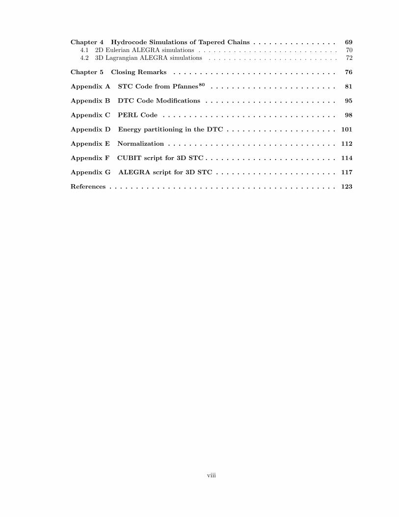
Chapter 4 Hydrocode Simulations of Tapered Chains . . . . . . . . . . . . . . . . 694.1 2D Eulerian ALEGRA simulations . . . . . . . . . . . . . . . . . . . . . . . . . . . . 704.2 3D Lagrangian ALEGRA simulations . . . . . . . . . . . . . . . . . . . . . . . . . . 72

Chapter 5 Closing Remarks . . . . . . . . . . . . . . . . . . . . . . . . . . . . . . . 76

Appendix A STC Code from Pfannes80 . . . . . . . . . . . . . . . . . . . . . . . . 81

Appendix B DTC Code Modifications . . . . . . . . . . . . . . . . . . . . . . . . . 95

Appendix C PERL Code . . . . . . . . . . . . . . . . . . . . . . . . . . . . . . . . . 98

Appendix D Energy partitioning in the DTC . . . . . . . . . . . . . . . . . . . . . 101

Appendix E Normalization . . . . . . . . . . . . . . . . . . . . . . . . . . . . . . . . 112

Appendix F CUBIT script for 3D STC . . . . . . . . . . . . . . . . . . . . . . . . . 114

Appendix G ALEGRA script for 3D STC . . . . . . . . . . . . . . . . . . . . . . . 117

References . . . . . . . . . . . . . . . . . . . . . . . . . . . . . . . . . . . . . . . . . . . 123

viii

Abstract

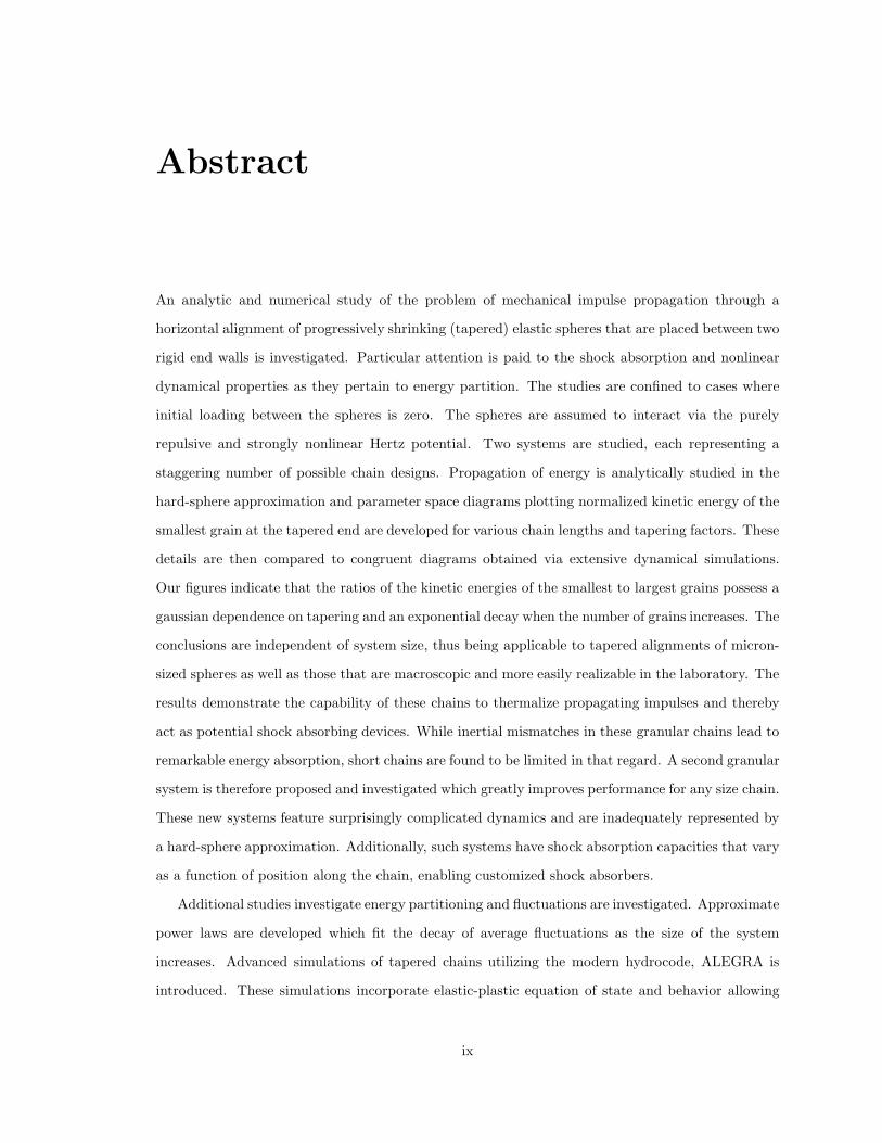
An analytic and numerical study of the problem of mechanical impulse propagation through a

horizontal alignment of progressively shrinking (tapered) elastic spheres that are placed between two

rigid end walls is investigated. Particular attention is paid to the shock absorption and nonlinear

dynamical properties as they pertain to energy partition. The studies are confined to cases where

initial loading between the spheres is zero. The spheres are assumed to interact via the purely

repulsive and strongly nonlinear Hertz potential. Two systems are studied, each representing a

staggering number of possible chain designs. Propagation of energy is analytically studied in the

hard-sphere approximation and parameter space diagrams plotting normalized kinetic energy of the

smallest grain at the tapered end are developed for various chain lengths and tapering factors. These

details are then compared to congruent diagrams obtained via extensive dynamical simulations.

Our figures indicate that the ratios of the kinetic energies of the smallest to largest grains possess a

gaussian dependence on tapering and an exponential decay when the number of grains increases. The

conclusions are independent of system size, thus being applicable to tapered alignments of micron-

sized spheres as well as those that are macroscopic and more easily realizable in the laboratory. The

results demonstrate the capability of these chains to thermalize propagating impulses and thereby

act as potential shock absorbing devices. While inertial mismatches in these granular chains lead to

remarkable energy absorption, short chains are found to be limited in that regard. A second granular

system is therefore proposed and investigated which greatly improves performance for any size chain.

These new systems feature surprisingly complicated dynamics and are inadequately represented by

a hard-sphere approximation. Additionally, such systems have shock absorption capacities that vary

as a function of position along the chain, enabling customized shock absorbers.

Additional studies investigate energy partitioning and fluctuations are investigated. Approximate

power laws are developed which fit the decay of average fluctuations as the size of the system

increases. Advanced simulations of tapered chains utilizing the modern hydrocode, ALEGRA is

introduced. These simulations incorporate elastic-plastic equation of state and behavior allowing

ix

us to probe very large loading of tapered chains. This leads into the discussion of our continuing

work beyond this dissertation including the design of a shock absorbing panel. Historical context is

provided which has lead researchers to begin looking seriously at these alluring properties of granular

or discretized systems.

x

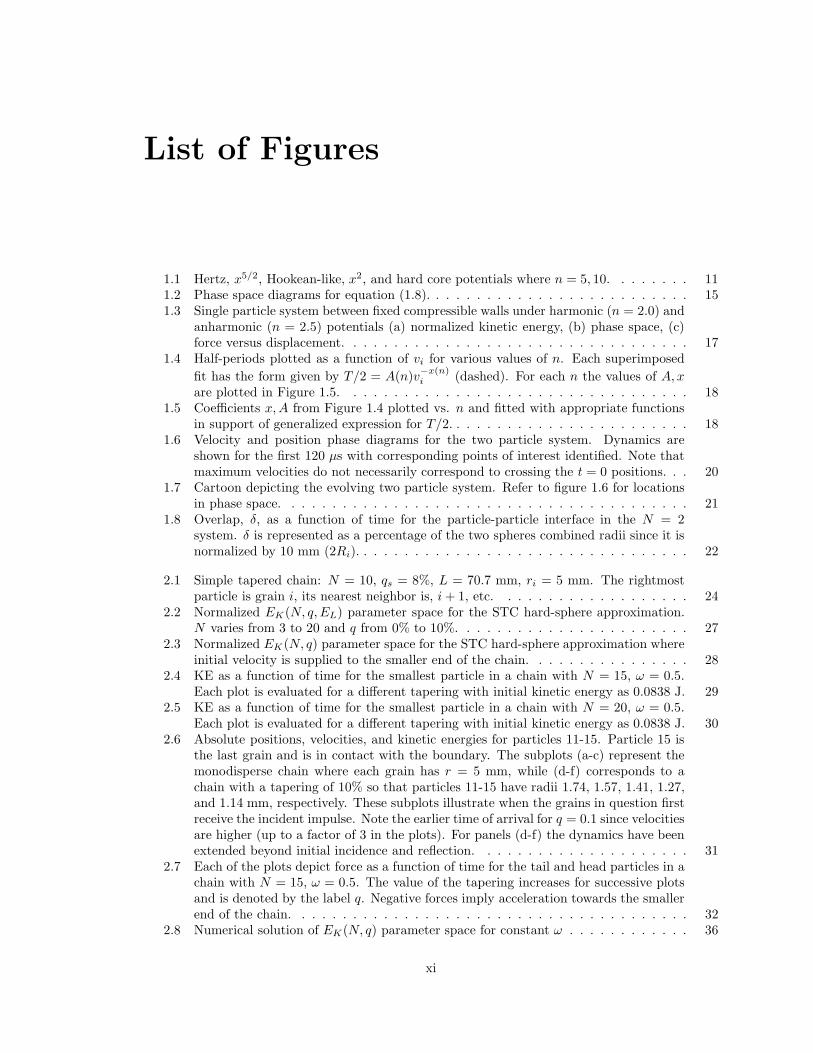
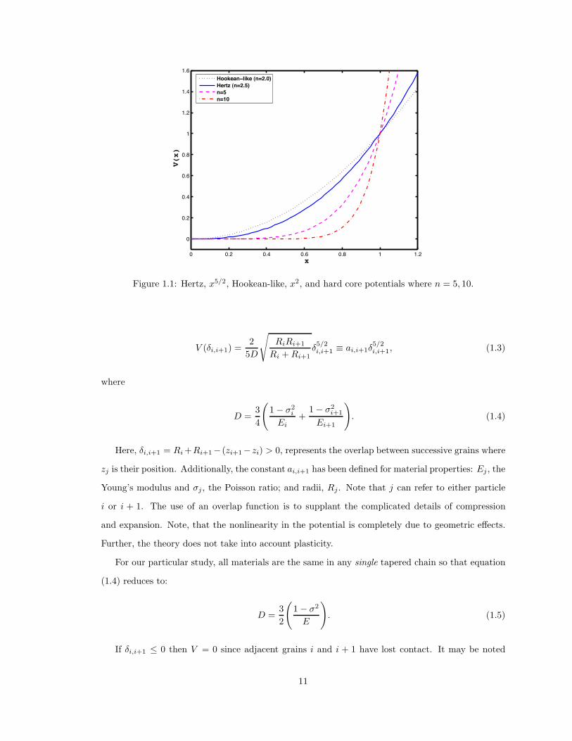
List of Figures

1.1 Hertz, x5/2, Hookean-like, x2, and hard core potentials where n = 5, 10. . . . . . . . 111.2 Phase space diagrams for equation (1.8). . . . . . . . . . . . . . . . . . . . . . . . . . 151.3 Single particle system between fixed compressible walls under harmonic (n = 2.0) and

anharmonic (n = 2.5) potentials (a) normalized kinetic energy, (b) phase space, (c)force versus displacement. . . . . . . . . . . . . . . . . . . . . . . . . . . . . . . . . . 17

1.4 Half-periods plotted as a function of vi for various values of n. Each superimposedfit has the form given by T/2 = A(n)v!x(n)

i (dashed). For each n the values of A, xare plotted in Figure 1.5. . . . . . . . . . . . . . . . . . . . . . . . . . . . . . . . . . 18

1.5 Coe"cients x, A from Figure 1.4 plotted vs. n and fitted with appropriate functionsin support of generalized expression for T/2. . . . . . . . . . . . . . . . . . . . . . . . 18

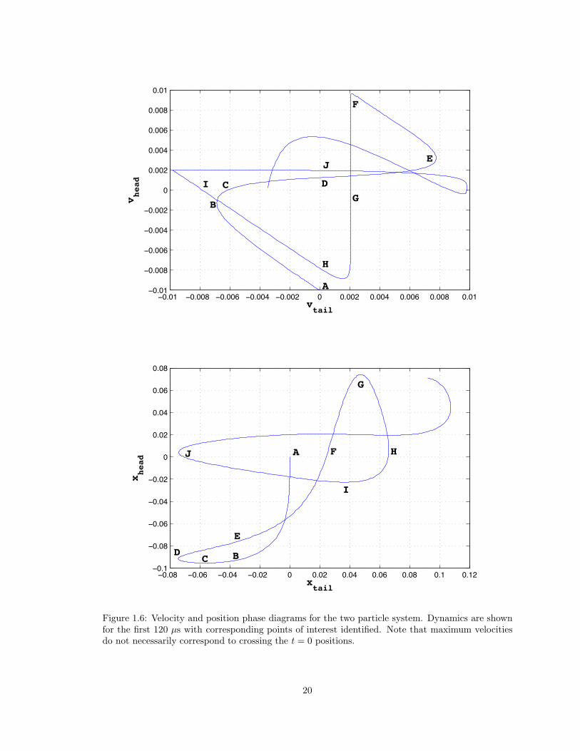
1.6 Velocity and position phase diagrams for the two particle system. Dynamics areshown for the first 120 µs with corresponding points of interest identified. Note thatmaximum velocities do not necessarily correspond to crossing the t = 0 positions. . . 20

1.7 Cartoon depicting the evolving two particle system. Refer to figure 1.6 for locationsin phase space. . . . . . . . . . . . . . . . . . . . . . . . . . . . . . . . . . . . . . . . 21

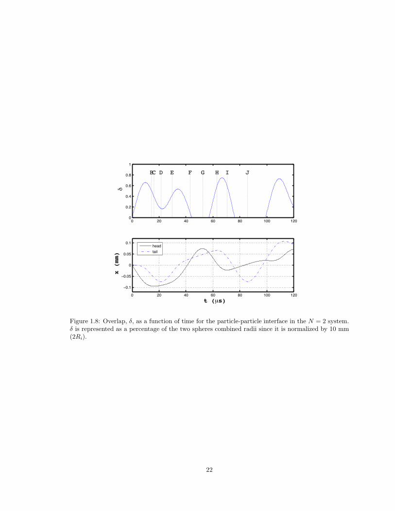
1.8 Overlap, !, as a function of time for the particle-particle interface in the N = 2system. ! is represented as a percentage of the two spheres combined radii since it isnormalized by 10 mm (2Ri). . . . . . . . . . . . . . . . . . . . . . . . . . . . . . . . . 22

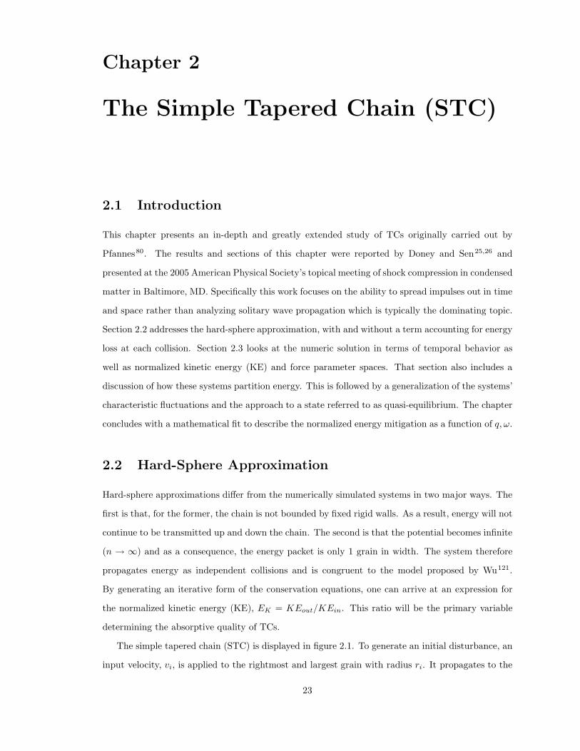
2.1 Simple tapered chain: N = 10, qs = 8%, L = 70.7 mm, ri = 5 mm. The rightmostparticle is grain i, its nearest neighbor is, i + 1, etc. . . . . . . . . . . . . . . . . . . 24

2.2 Normalized EK(N, q, EL) parameter space for the STC hard-sphere approximation.N varies from 3 to 20 and q from 0% to 10%. . . . . . . . . . . . . . . . . . . . . . . 27

2.3 Normalized EK(N, q) parameter space for the STC hard-sphere approximation whereinitial velocity is supplied to the smaller end of the chain. . . . . . . . . . . . . . . . 28

2.4 KE as a function of time for the smallest particle in a chain with N = 15, " = 0.5.Each plot is evaluated for a di!erent tapering with initial kinetic energy as 0.0838 J. 29

2.5 KE as a function of time for the smallest particle in a chain with N = 20, " = 0.5.Each plot is evaluated for a di!erent tapering with initial kinetic energy as 0.0838 J. 30

2.6 Absolute positions, velocities, and kinetic energies for particles 11-15. Particle 15 isthe last grain and is in contact with the boundary. The subplots (a-c) represent themonodisperse chain where each grain has r = 5 mm, while (d-f) corresponds to achain with a tapering of 10% so that particles 11-15 have radii 1.74, 1.57, 1.41, 1.27,and 1.14 mm, respectively. These subplots illustrate when the grains in question firstreceive the incident impulse. Note the earlier time of arrival for q = 0.1 since velocitiesare higher (up to a factor of 3 in the plots). For panels (d-f) the dynamics have beenextended beyond initial incidence and reflection. . . . . . . . . . . . . . . . . . . . . 31

2.7 Each of the plots depict force as a function of time for the tail and head particles in achain with N = 15, " = 0.5. The value of the tapering increases for successive plotsand is denoted by the label q. Negative forces imply acceleration towards the smallerend of the chain. . . . . . . . . . . . . . . . . . . . . . . . . . . . . . . . . . . . . . . 32

2.8 Numerical solution of EK(N, q) parameter space for constant " . . . . . . . . . . . . 36

xi

2.9 Numerical solution of F (N, q) parameter space for constant " . . . . . . . . . . . . . 372.10 Di!erence plot of the lossless KE parameter spaces for the hard-sphere approximation

(Figure 2.2a) and numerical solution (Figure 2.8a). Note that the azimuthal view hasbeen rotated 180 degrees for clarity. . . . . . . . . . . . . . . . . . . . . . . . . . . . 37

2.11 Energy partitioning for STCs where N = {3, 8, 14, 20} represents the number ofspheres and qs = {0.0, 0.05, 0.1} is the tapering. Noisy plots resembling panel l in-dicate shock absorbing systems while those similar to panel j transmits an impulseas a solitary wave — essentially without loss. Panels a-c represent e"cient energyconversion systems. . . . . . . . . . . . . . . . . . . . . . . . . . . . . . . . . . . . . . 38

2.12 Normalized KE for N = 3, qs = 0.05. E1 represents the head of the chain and input;E2 is the central bead; and E3 is the tail. Note the periodicity of the system resultingin a recurrence time of just under 80 µs. . . . . . . . . . . . . . . . . . . . . . . . . . 39

2.13 Instantaneous kinetic energy per grain for N = 15, t = 52µs and selected tapering. . 402.14 Normalized kinetic energy landscape. Vertical axes represents the particle id while

the horizontal axis is time out to 1000 µs. . . . . . . . . . . . . . . . . . . . . . . . . 492.15 Velocity distribution with superimposed Gaussian fit for each particle in a STC with

N = 4, q = 0. Particle 1 represents the end of the chain and particle 4 represents thehead where the initial impulse was applied. . . . . . . . . . . . . . . . . . . . . . . . 50

2.16 Velocity distribution with superimposed Gaussian fit for each particle in a STC withN = 20, q = 0. Particle 1 represents the end of the chain and particle 20 representsthe head where the initial impulse was applied. . . . . . . . . . . . . . . . . . . . . . 51

2.17 Average kinetic energy of the system as a function of n and N . . . . . . . . . . . . . 522.18 Average kinetic energy of the system determined from simulation (circles) and theo-

retical expectation by the Virial Theorem (dashed). . . . . . . . . . . . . . . . . . . 522.19 Partition of energy by grain number for several STCs where N = {3, 8, 14, 20} and

q = {0, 0.05, 0.1} at t = 100µs. The red line indicates the theoretical expectation that< KEn >= n/(n+2)

N . . . . . . . . . . . . . . . . . . . . . . . . . . . . . . . . . . . . . 532.20 Partition of energy by grain number for several STCs where N = {3, 8, 14, 20} and

q = {0, 0.05, 0.1} at t = 500µs. The red line indicates the theoretical expectation that< KEn >= n/(n+2)

N . . . . . . . . . . . . . . . . . . . . . . . . . . . . . . . . . . . . . 532.21 Partition of energy by grain number for several STCs where N = {3, 8, 14, 20} and

q = {0, 0.05, 0.1} at t = 1000µs. The red line indicates the theoretical expectationthat < KEn >= n/(n+2)

N . . . . . . . . . . . . . . . . . . . . . . . . . . . . . . . . . . 542.22 Fluctuations as a function of time and n for N = 100, q = 0. . . . . . . . . . . . . . . 552.23 (a) Variation of < F > with N for various n and fitting function. (b) Variation

(scatter) of k with n. (c) Variation of A with n and corresponding fitting function.(d) Variation of B with n and corresponding fitting function. . . . . . . . . . . . . . 56

2.24 < F > as a function of n for various N determined from simulation (circles). Derivedfitting function < F >=< F (n, N) > is superimposed (dashed) in each panel. n = 2data is excluded as it doesn’t fit the function. . . . . . . . . . . . . . . . . . . . . . . 57

2.25 |vmax| as a function of time for N = 16, 18, 20, 50. . . . . . . . . . . . . . . . . . . . . 582.26 The Simulated and Modeled STC. . . . . . . . . . . . . . . . . . . . . . . . . . . . . 59

3.1 Several example DTCs created by varying f and qd for constant N = 13. . . . . . . . 613.2 Normalized kinetic energy surfaces, EK ! KOUT /KIN , for the decorated chain under

the hard sphere approximation as functions of the number of spheres, N , fractionalsize of interstitial sphere, f , and tapering, qd. . . . . . . . . . . . . . . . . . . . . . . 65

3.3 Numerically-produced normalized kinetic energy surfaces, EK ! KOUT /KIN , for thedecorated chain as functions of the number of spheres, N , fractional size of interstitialsphere, f , and tapering, qd. Several sample chains are identified in panels (d-i). . . . 67

3.4 Instantaneous kinetic energy per grain for various DTC configurations at t = 52µswhere qd = {0, 0.05, 0.1} and f = {1.0, 0.7, 0.3}. . . . . . . . . . . . . . . . . . . . . . 68

4.1 Computational domain and problem setup for the ALEGRA simulation. . . . . . . . 70

xii

4.2 Evolution of |#xx|. Color scale is logarithmic. . . . . . . . . . . . . . . . . . . . . . . 714.3 Basic 3D simulation of a TC. Note that the bulk behavior of the spheres is consistent

with expectation even though dynamics take place on a elemental or nodal basis. Asmall amount of plastic flow is visible. . . . . . . . . . . . . . . . . . . . . . . . . . . 72

4.4 Velocity of the head particle as a function of time for both EOM and ALEGRAsimulations where N = 5, q = 0.07 and restitutive losses are neglected. . . . . . . . . 73

4.5 Time elapsed sequence where the initial velocity of the left-most grain has been in-creased to 500 m/s (red). The remaining spheres are initially stationary (blue). . . . 75

5.1 Schematic of what a tapered chain armor panel might look like. . . . . . . . . . . . . 78

D.1 Instantaneous kinetic energy per grain for various DTC configurations at t = 10µswhere qd = {0, 0.05, 0.1} and f = {1.0, 0.7, 0.3}. . . . . . . . . . . . . . . . . . . . . . 102










xiii

Chapter 1

Introduction

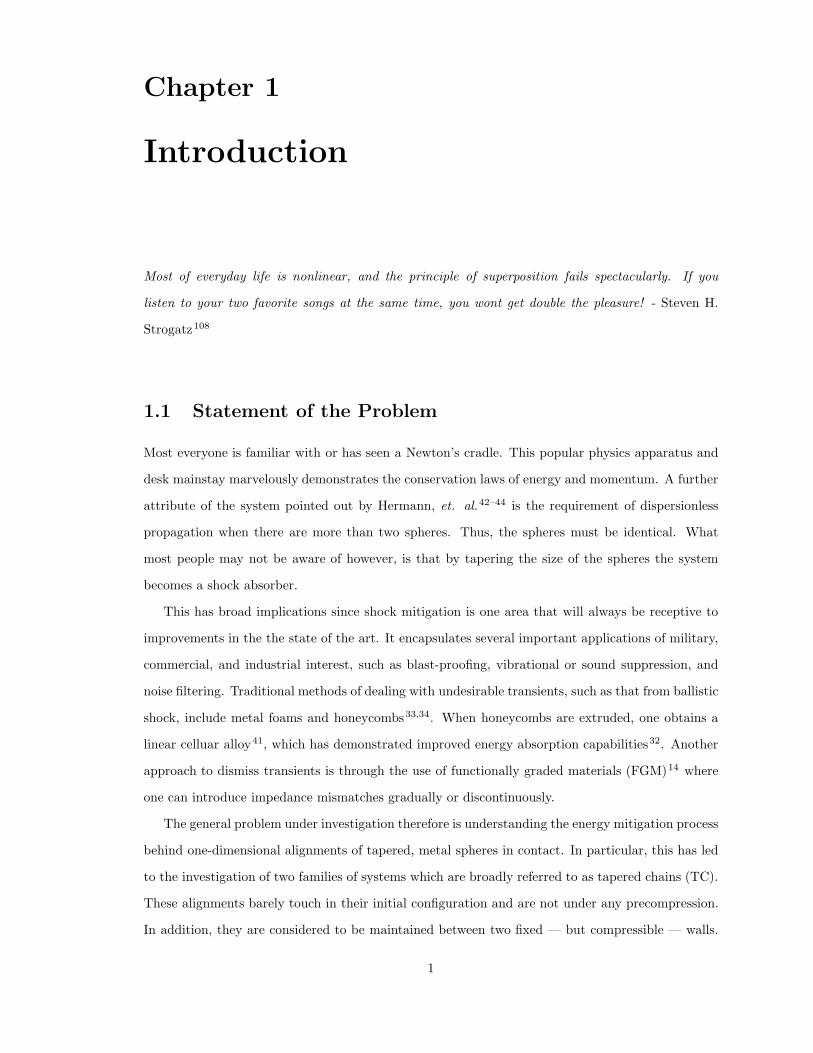
Most of everyday life is nonlinear, and the principle of superposition fails spectacularly. If you

listen to your two favorite songs at the same time, you wont get double the pleasure! - Steven H.

Strogatz108

1.1 Statement of the Problem

Most everyone is familiar with or has seen a Newton’s cradle. This popular physics apparatus and

desk mainstay marvelously demonstrates the conservation laws of energy and momentum. A further

attribute of the system pointed out by Hermann, et. al.42–44 is the requirement of dispersionless

propagation when there are more than two spheres. Thus, the spheres must be identical. What

most people may not be aware of however, is that by tapering the size of the spheres the system

becomes a shock absorber.

This has broad implications since shock mitigation is one area that will always be receptive to

improvements in the the state of the art. It encapsulates several important applications of military,

commercial, and industrial interest, such as blast-proofing, vibrational or sound suppression, and

noise filtering. Traditional methods of dealing with undesirable transients, such as that from ballistic

shock, include metal foams and honeycombs33,34. When honeycombs are extruded, one obtains a

linear celluar alloy41, which has demonstrated improved energy absorption capabilities32. Another

approach to dismiss transients is through the use of functionally graded materials (FGM)14 where

one can introduce impedance mismatches gradually or discontinuously.

The general problem under investigation therefore is understanding the energy mitigation process

behind one-dimensional alignments of tapered, metal spheres in contact. In particular, this has led

to the investigation of two families of systems which are broadly referred to as tapered chains (TC).

These alignments barely touch in their initial configuration and are not under any precompression.

In addition, they are considered to be maintained between two fixed — but compressible — walls.

1

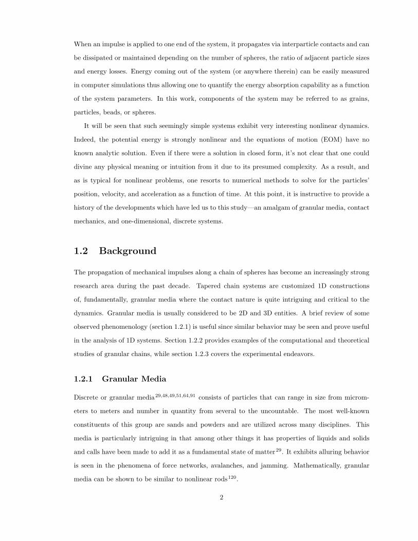
When an impulse is applied to one end of the system, it propagates via interparticle contacts and can

be dissipated or maintained depending on the number of spheres, the ratio of adjacent particle sizes

and energy losses. Energy coming out of the system (or anywhere therein) can be easily measured

in computer simulations thus allowing one to quantify the energy absorption capability as a function

of the system parameters. In this work, components of the system may be referred to as grains,

particles, beads, or spheres.

It will be seen that such seemingly simple systems exhibit very interesting nonlinear dynamics.

Indeed, the potential energy is strongly nonlinear and the equations of motion (EOM) have no

known analytic solution. Even if there were a solution in closed form, it’s not clear that one could

divine any physical meaning or intuition from it due to its presumed complexity. As a result, and

as is typical for nonlinear problems, one resorts to numerical methods to solve for the particles’

position, velocity, and acceleration as a function of time. At this point, it is instructive to provide a

history of the developments which have led us to this study—an amalgam of granular media, contact

mechanics, and one-dimensional, discrete systems.

1.2 Background

The propagation of mechanical impulses along a chain of spheres has become an increasingly strong

research area during the past decade. Tapered chain systems are customized 1D constructions

of, fundamentally, granular media where the contact nature is quite intriguing and critical to the

dynamics. Granular media is usually considered to be 2D and 3D entities. A brief review of some

observed phenomenology (section 1.2.1) is useful since similar behavior may be seen and prove useful

in the analysis of 1D systems. Section 1.2.2 provides examples of the computational and theoretical

studies of granular chains, while section 1.2.3 covers the experimental endeavors.

1.2.1 Granular Media

Discrete or granular media29,48,49,51,64,91 consists of particles that can range in size from microm-

eters to meters and number in quantity from several to the uncountable. The most well-known

constituents of this group are sands and powders and are utilized across many disciplines. This

media is particularly intriguing in that among other things it has properties of liquids and solids

and calls have been made to add it as a fundamental state of matter29. It exhibits alluring behavior

is seen in the phenomena of force networks, avalanches, and jamming. Mathematically, granular

media can be shown to be similar to nonlinear rods120.

2

Granular media (in any number of dimensions) has been intensely investigated for understanding

wave propagation1. Much of this has been in regard to understanding sound propagation. It has

become such a curiosity since, in 2D or 3D, not all grains are under contact so various contact or

force networks are formed. That is, only particles in contact admit mechanical energy propagation

and the identified network visually appears dendritic. However, when one slightly shakes the gran-

ular bed, the network is completely changed. This is important for improving imaging of buried

objects, such as munitions, in various soils. Sinkovits and Sen101,102 presented simulations on the

vertical propagation of weak and strong impulses in deep gravitationally compacted columns. In

such asymmetrically loaded columns, the sound velocity, c, increases with depth as c " z1/6, where

z is the depth. Sen101 extended the study to include voids and mass impurities. The inclusion of

the latter caused backscatter at the defects even though the chains were monodisperse (identically-

sized). This then prompted further study by Sen, et. al.98 to report it as a possible mechanism for

the detection of buried impurities, such as mines, bones, lost treasure, etc. The specific nature of

the propagation59 and backscattering60 was investigated more thoroughly by Manciu who correlated

the results into a dissertation58 on nonlinear acoustics in granular media.

It is intriguing and suggestive that, conceptually, granular media can be envisioned as the inverse

of a porous material. In a porous material, there are gaseous (air) voids within a solid matrix. For

dry granular media, the reverse is true: solid (grains) voids exist within a gaseous matrix. This is

an interesting comparison to draw because the considerable amount of work required to collapse the

voids in a porous material makes it a favorable technology against ballistic shock32.

1.2.2 Granular Chains: Computational and Theoretical studies

Since the Hertz potential is strongly nonlinear, a review of nonlinear methods and waves was in

order. It was believed that such resources would prove valuable in the analysis and approxi-

mation of TCs. While there are an inordinate number of books available on nonlinear dynam-

ics39,40,67,68,73,74,105,106,108,114, they generally focus on perturbation-type solutions and analysis of

the resulting nonlinear and chaotic waves9,70,106,112,118.

In most cases, undamped, damped and forced oscillators, such as the Van der Pol and Du"ng

oscillators, are examined in detail along with the their behaviors in phase space. The behavior of

nonlinear waves is introduced through the simplest forms of dispersive and di!usive equations9,73:

the Korteweg deVries (KdV) equation52,122 and Burgers equation15, respectively. The KdV equation

for example admits solitary wave solutions.

3

A shortcoming of these works is that none of them address fractional power exponents. Mickens67

and Gottlieb38 have the most relevant analytic work on oscillators with fractional power nonlinear-

ities. Their approach uses the so-called Harmonic Balance technique66 for periodic systems which

matches the coe"cients in a truncated Fourier series to determine the frequency of oscillation. A

benefit of the method is that it does not require a perturbation parameter so it is applicable to

strongly nonlinear systems. Harmonic Balance however seems to be limited to specific problems.

Solitary waves (SW) are intriguing because they propagate over very large distances with negligi-

ble dissipation86. The first known observation was reported in 1844 by Russell92 who noticed water

waves in a shallow canal propagate without loss over several miles. Ultimately they were broken

apart by branching of the channel. An exhaustive historical account of the theoretical development

of SWs is expounded by Sander93. It should be noted that when SWs collide and emerge unchanged

they are referred to as solitons because of the similarity to particles83.

SWs were of particular interest in past studies since, for monodisperse chains, they are the

mode of energy transport77,95. Sen and Pfannes demonstrated that it takes about 15 grains for

the SW to form in such a chain. Considerable e!ort has been spent investigating the phenomena

numerically and experimentally. Nesterenko first arrived at an analytic solution of a precompressed,

monodispersed system using anharmonic and long wavelength approximations of the EOM75. The

equations were then reduced to a form similar to the KdV equation52 whereby SWs35 were observed.

Lattice dynamics are dependent on the type of interaction potential chosen. The 1D (atomic)

lattice and coupled oscillators immediately stand out where Morse7, exponential114, and other

nonlinear (pertubative) potentials have been used. A common observable in most cases is the

existence of solitary waves. In point, Toda114 obtained exact (soliton) solutions in a one-dimensional

lattice with exponential interactions in closed form.

Additionally, one of the more curious behaviors in granular chains is that of inelastic collapse63.

This occurs when the separation between particles drops to zero due to a competition between the

number of particles in the system and energy losses. Since the velocity of the particles involved in

the collapse decay, this would be an ideal phenomenon to exploit for shock mitigation purposes. We

have not yet investigated this.

In the following subsections, specific developments of FPU and mixed harmonic-anharmonic

potentials and the overlap potential are discussed. This follows with some review of work focused

on equipartition and equilibrium in such systems.

4

FPU and mixed harmonic-anharmonic potentials

Fermi, Pasta, and Ulam30 (FPU) are credited with the first computational study on energy sharing

between modes where quadratic, cubic, and broken linear potentials were used. As a side note, the

FPU 1D lattice has become a testbed for looking at various physics such as impulse propagation,

defining temperature, and energy sharing among modes. An enormous body of literature is available

on the subject. They noticed that upon the inclusion of such nonlinearities, energy that was initially

fed to the lower mode became mixed among several lower order modes, but then returned to the

lowest mode. Such recurrence can indicate hidden periodicities. These results are in contrast to a

purely linear problem. For example, if one were to excite the lowest mode only in a general solution

to the (linear) wave equation, the energy would stay in the fundamental mode for all time78.

The approach to equilibrium in discrete systems has been a topic of considerable interest for quite

some time and the open literature is replete with examples. In general one wishes to understand

whether the system reaches equilibrium by how energy is shared among the sites in a 1D lattice

and how long it takes to do so. Typically the systems studied have a Hamiltonian of the form,

H = H0 + $H1 where H0 represents the linear portion, H1 represents nonlinear (sin(x), x3, x4,

etc.) terms and $ is a tuning parameter. In this sense, many of the perturbation techniques in

previous references may be applied. An additional benefit is that one can monitor how energy is

shared between normal modes from the linear system and the e!ects of adding a small nonlinear

perturbation.

Fermi addressed the question of energy equipartition30 and Toda114 points out lucidly,

Fermi did some work on the ergodic problem when he was young, and when electronic

computers were developed he came back to this as one of the problems computers might

solve. He thought that if one added a nonlinear term to the force between particles in

a one-dimensional lattice, energy would flow from mode to mode eventually leading the

system to a statistical equilibrium state where the energy is shared equally among the

modes.

This investigation sparked a broad literature base24,85 and a description of some of this work

follows. Ford and Waters have addressed the issue of equipartition of FPU systems in several

exhaustive papers. Ford31 used a perturbation technique to show that the chain originally used

by FPU didn’t equipartition energy because of an inappropriate choice of frequencies. He argues

that for weakly coupled oscillator system — with linear and nonlinear terms — one should expect

(internal) resonance and energy sharing when the sum of harmonic frequencies is approximately

5

zero.

Tobolsky et. al.113 observed equipartition for several lattice models. They commented however

that the probability of a given deviation of kinetic and potential energies from one-half approaches

a limit that decreases with increasing N . For a deviation, x, with probability of 1% being exceeded,

I measure this decay (based on their data) as x = 3/(4#

N), where N is the number of particles.

Boccheri et. al.10 numerically investigate a one dimensional chain of particles with nearest neigh-

bor interactions using a Lennard-Jones potential. They conclude that when the particle vibration

energy exceeds a few percent of the depth of the potential well, equipartition of energy among the

normal modes is satisfied in the time average. This is in contrast to the Toda lattice114 where

exponential interactions were not compatible with equipartition of energy in the time average.

Rosas and Lindenberg89 studied pulse propagation in FPU lattices (where only quartic nonlin-

earities were considered). They varied the input velocity governing whether harmonic or anharmonic

terms dominate (since the velocity of nonlinear waves is amplitude dependent). They concluded that

the pulse width is not an appropriate measure of the way a pulse spreads in a purely anharmonic

lattice but rather it measures the span over which a series of decreasing velocity pulses exist. This

was an extension of an earlier, more comprehensive, study by Sarmiento et. al.94. They measured

pulse propagation in isolated FPU chains and also those coupled to heat baths of zero and finite

temperatures as well as 2d isolated arrays.

Finally, one of the more recent discoveries has been the observation of “breathers” —periodic and

localized nonlinear lattice excitations81. These spontaneous and long-lived localizations of energy

result from competition between nonlinearity and space discreteness81. Another typical requirement

is for the array to be cooled at the boundaries. Essentially, all energy dissipation takes place at the

end points and is equivalent to the physical situation of a surface cooling much faster than the bulk

of the medium. Breathers emerge from such configurations where the lattice is initially thermalized

and is an evolved form of self-excited oscillations—another nonlinear behavior. In this report,

such behavior has not been observed because free-end BCs nor boundary-only cooling have been

considered. Further conclusions of Piazza, et. al. were that breather mobility is impacted if space

discreteness (i.e. weak nearest neighbor interaction or restoration potential) is too large.

Overlap potential

The study of granular columns is dominated by the Hertz potential — see equation (1.3). This is

a special case of the more generalized overlap potential, !n. The overlap potential is quite distinct

from FPU and other lattice potentials. First, they lack a harmonic term — that is, they are strongly

6

nonlinear. Thus, nonlinear perturbation methods fail when looking for a solution. Second, and most

important, is that they lack a restoring term. So even if the overlap potential is considered with a

“harmonic” exponent, !2, the chain is very dissimilar from a simple harmonic system.

Nesterenko is considered to be the pioneer of theoretical, computational, and experimental studies

of SW in Hertzian chains. His work is found compiled in chapter one of his book76 which includes

translations of his Russian publications. He was the first to observe solitons in Hertzian chains75

and also dubbed such granular chains a “sonic vacuum,” since particles can lose contact when

precompression in the chain is not considered.

The phenomenology of SWs in granular chains was addressed specifically in several computa-

tional papers by Sen and Manciu61,95. For long, uncompressed chains—where boundary e!ects

are ignored—they observed that SWs are the mode of energy transport when n > 2. They used

a combination of computational and analytic arguments to guess a form of the SW as, %n(z) =

$(A/2) tanh[fn(z)/2], where the fn(z) represents a series expansion in z and requires calculation of

the coe"cients for each term in the series. Their solution agrees quite well with simulations when

only the first three coe"cients are solved. Thus they were able to obtain displacement, velocity, and

acceleration functions for the SW. This approach di!ers from that of Nesterenko’s long wave, or con-

tinuum, approximation in that zero precompression is considered and the EOM are not linearized.

Their subsequent publication investigates how propagation of the SW is a!ected by dissipation and

disorder for arbitrary power-law repulsive potentials, !n. They conclude that even in the presence of

disorder, a SW propagates—maintaining its width while the amplitude decreases exponentially with

distance. The attenuation is common whether energy loss is caused by restitution or velocity-based

friction, or from multiple backscattering events due to randomly-sized particles in the chain. The

attenuation commonality thus enables one to choose an energy loss mechanism that is convenient.

An additional note of interest is that as the SW propagates in the disordered medium, part of the

energy remains behind the leading edge in the form of noise which doesn’t interfere with the SW.

Since wave velocity is a function of amplitude and noise has a much smaller amplitude, the SW

outpaces noise.

In a subsequent study, Sen et. al.97 inquired as to whether it was possible to convert an impulse

into thermal energy. Based on supporting computational studies they concluded that when particle

radii taper to smaller sizes, the traveling SW must get “squeezed” into a smaller size. The SW

consequently loses its reflective symmetry and is destroyed. More specifically, the SW is rapidly

attenuated and undergoes dispersion due to progressively smaller and faster particle masses. That

the energy transport mechanism was found to be disabled by tapered chains led to many exciting

7

questions and became the foundation for this dissertation. Curiously, Poschel and Brilliantov82

found that by using a constant coe"cient of restitution, one obtains optimum energy transmission

if the mass of each particle is prescribed by an exponentially decreasing function.

Wu121 uses an independent collision or binary collision model to understand wave propagation

in uniform (monodisperse) and tapered chains. In such a system, energy is always confined to a

single particle. This model is analogous to hard-spheres which is derived in sections 2.2 and 3.2.

Rosas and coauthors perform a series of relevant studies with Hertzian chains. In the first work87,

the authors look at how propagation and backscattering between two granules is a!ected by the type

(kinetic or hydrostatic) of friction and its magnitude. Among their conclusions is that friction on

the second granule is responsible for backscattering. And in sum, they found a drastic asymmetry

between backscattering and propagation for various frictional states. This work is followed up88 by

concluding that a binary collision model is quantitatively correct for (hard) potentials where n % 3.

This is because the pulse is so narrow that at any given moment the energy is concentrated in just

a few particles. Indeed they reiterate that in the continuum approximation (N & '), the pulse

width goes as & =!

(6(n $ 2))2/n(n $ 1). Subsequently, the authors investigate frictional e!ects

further for cylindrical and spherical granules90. An interesting result for the cylindrical case is that

the backscatter velocity for finite friction is greater than that when it is neglected. They also find an

exponential decay to the velocity of backscatter velocity as well as energy. The latter is in agreement

with findings in this report (see figure 2.26(a)—T (") decays exponentially)

In more recent work, a new type of steady-state behavior, quasi-equilibrium99,100, has been

observed. The findings of the authors’ are summarized as follows. Without a linear, harmonic term

in the potential, grains do not exhibit simple harmonic motion which produces sound waves —

indeed a restoring term is required. This is the “sonic vacuum” Nesterenko referred to. As such,

information or energy is transmitted by groups of particles rather than individual grains. When

an interaction with a boundary occurs, energy remains nucleated at the site, some of which goes

into recreating an attenuated SW while the rest rattles about, creating secondary SW (SSW)57 of

very small amplitude. Since SW width is controlled by n, the system transmits energy via SW

and SSWs such that (1) large and small SW collisions exchange momenta if parallel114; (2) they

undergo breakdown and reconstruction with attenuation by antiparallel collisions or interaction

with a boundary59. At large times, it was found that the system tends towards a Gaussian velocity

distribution. Apparently in all cases studied, the process of reconstructing a SW is imperfect. There

is attenuation every time a boundary is encountered, the remaining energy goes into making SSW.

Mohan and Sen69 investigated similar questions for mass-spring systems with quartic interactions

8

for both periodic and rigid, perfectly reflecting boundary conditions. They found that for the purely

harmonic mass-spring chain, energy quickly approaches E0/N per particle, thus equipartition was

achieved. In the mixed harmonic/anharmonic case, the presence of harmonicity tends to “wash-

out” nonlinear e!ects. Therefore the comparative strengths of linear and nonlinear terms become

an important factor in determining the relaxation time.

1.2.3 Granular Chains: Experimental Work

Some of the earliest experimental work focused on the establishment of the restitutive coe"cient

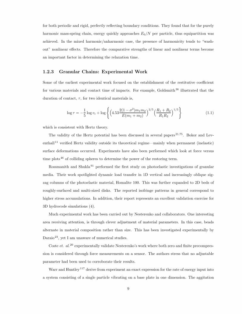
for various materials and contact time of impacts. For example, Goldsmith36 illustrated that the

duration of contact, ' , for two identical materials is,

log ' = $15

log vi + log

"#4.53

2(1 $ #2)m1m2

E(m1 + m2)

$2/5#R1 + R2

R1R2

$1/5%

(1.1)

which is consistent with Hertz theory.

The validity of the Hertz potential has been discussed in several papers21,75. Bokor and Lev-

enthall11 verified Hertz validity outside its theoretical regime—mainly when permanent (inelastic)

surface deformations occurred. Experiments have also been performed which look at force versus

time plots46 of colliding spheres to determine the power of the restoring term.

Rossmanith and Shukla91 performed the first study on photoelastic investigations of granular

media. Their work spotlighted dynamic load transfer in 1D vertical and increasingly oblique zig-

zag columns of the photoelastic material, Homalite 100. This was further expanded to 2D beds of

roughly-surfaced and multi-sized disks. The reported isofringe patterns in general correspond to

higher stress accumulations. In addition, their report represents an excellent validation exercise for

3D hydrocode simulations (4).

Much experimental work has been carried out by Nesterenko and collaborators. One interesting

area receiving attention, is through clever adjustment of material parameters. In this case, beads

alternate in material composition rather than size. This has been investigated experimentally by

Daraio23, yet I am unaware of numerical studies.

Coste et. al.20 experimentally validate Nesterenko’s work where both zero and finite precompres-

sion is considered through force measurements on a sensor. The authors stress that no adjustable

parameter had been used to corroborate their results.

Warr and Huntley117 derive from experiment an exact expression for the rate of energy input into

a system consisting of a single particle vibrating on a base plate in one dimension. The aggitation

9

coupled with the rate of energy dissipation allowed the steady state of the system to be determined

energetically. In particular they found, Ep = 1.7mpV 2/(1 $ $), where V is the base plate velocity,

$ the coe"cient of restitution, and Ep and mp are the particle energy and mass, respectively. Ad-

ditional research56 investigates the phase behavior—fluidization and condensation (also known as

clumping)—of a column of beads under similar vibrating plates.

Nakagawa et. al.72 experimentally confirm impulse dispersion in tapered chains. They further

provide a derived measurement for the coe"cient of restitution of 0.95 and account for discrepancies

in the computational studies by arguing that some of the energy is transferred to rotational degrees

of freedom. Experimental work has also focused on the observation of SWs and their behavior at

boundaries50,65,104. With relevance to chapter 3, a “decorated tapered chain” prototype has very

recently been constructed for empirically testing and validating its shock mitigation capability2.

1.3 Mathematical Description of Problem

We define TCs (see for example figure 2.1) as 1-D granular arrays of elastic spheres that touch at a

single point in their initial state and grow to a disk under compression in the plane perpendicular

to the figure. The chains can be characterized by the number of grains, N , the successive decrease

in size of the grains or tapering, q, and restitutive or energy losses, ".

The Hamiltonian of the system is represented as,

H =12

&

i

mix2i +

&

i

V (!ni,i+1) (1.2)

where V (!ni,i+1) is the overlap potential. When n = 5/2, V is referred to as the Hertz potential and

is described in section 1.3.1. The equations of motion follow in section 1.3.2, resititutive losses in

section 1.3.3, relevant boundary and initial conditions in section 1.3.4, and the numeric approach to

solving the N equations of motion in section 1.3.5.

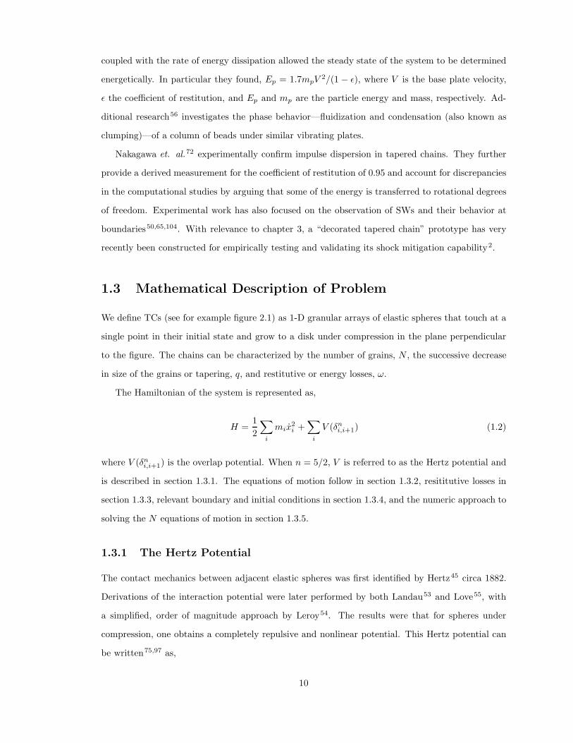
1.3.1 The Hertz Potential

The contact mechanics between adjacent elastic spheres was first identified by Hertz45 circa 1882.

Derivations of the interaction potential were later performed by both Landau53 and Love55, with

a simplified, order of magnitude approach by Leroy54. The results were that for spheres under

compression, one obtains a completely repulsive and nonlinear potential. This Hertz potential can

be written75,97 as,

10

0 0"2 0"4 0"% 0"& 1 1"2

0

0"2

0"4

0"%

0"&

1

1"2

1"4

1"%

x

V(x)

Hookean!like (n=2.0)Hertz (n=2.5)n=5n=10

Figure 1.1: Hertz, x5/2, Hookean-like, x2, and hard core potentials where n = 5, 10.

V (!i,i+1) =2

5D

'RiRi+1

Ri + Ri+1!5/2i,i+1 ! ai,i+1!

5/2i,i+1, (1.3)

where

D =34

(1 $ #2

i

Ei+

1 $ #2i+1

Ei+1

). (1.4)

Here, !i,i+1 = Ri +Ri+1$ (zi+1$zi) > 0, represents the overlap between successive grains where

zj is their position. Additionally, the constant ai,i+1 has been defined for material properties: Ej , the

Young’s modulus and #j , the Poisson ratio; and radii, Rj . Note that j can refer to either particle

i or i + 1. The use of an overlap function is to supplant the complicated details of compression

and expansion. Note, that the nonlinearity in the potential is completely due to geometric e!ects.

Further, the theory does not take into account plasticity.

For our particular study, all materials are the same in any single tapered chain so that equation

(1.4) reduces to:

D =32

(1 $ #2

E

). (1.5)

If !i,i+1 ( 0 then V = 0 since adjacent grains i and i + 1 have lost contact. It may be noted

11

that equation (1.3) describes a repulsive potential that grows faster than a quadratic—or Hookean-

like—form of !2i,i+1. The phrase, “Hookean-like” is used to stress the lack of a restoring term. The

Hertz repulsion is hence a nonlinear force. More specifically, the repulsion is softer than something

harmonic over short distances, but becomes steeper than a harmonic form with increasing compres-

sion. An extreme case would be the hard-sphere potential (n & '). These details are illustrated in

Figure 1.1 where V (x) is plotted for various values of n.

1.3.2 Equations of Motion

The EOM for grain mi at position zi is constructed from equation (1.3) as

mizi =52

*ai!1,i!

3/2i!1,i $ ai,i+1!

3/2i,i+1

+, (1.6)

where the dots imply di!erentiation with respect to time. Recall that !i,i+1 = Ri +Ri+1$(zi+1$zi)

represents the overlap of successive grains where zj is the position of a grain. Results have been

obtained for a large selection of chains consisting entirely of Ti6Al4V and SiC spheres. Arbitrarily,

we have chosen to use Ti6Al4V when restitutive losses are ignored (" = 0), and SiC otherwise. The

following material properties62 were assumed (where D is defined in equation (1.5)):

Table 1.1: Material PropertiesMaterial ((mg/mm3) D(mm2/kN) Occurence

SiC 3.2 0.003266 " )= 0Ti6Al4V 4.42 0.01206 " = 0

Note that the fundamental units of length, time, mass, and force in our simulations are the

millimeter, microsecond, milligram, and kilonewton, respectively. This is to minimize potential

rounding errors from small numbers.

1.3.3 Restitutive Losses

Real systems have various modes of energy dissipation—sliding, rolling, sound, etc. The literature

is replete with methods for invoking restitutive losses5,6,19, many of them velocity based109. For

simplicity, we have utilized the method of Walton and Braun116, where the coe"cient of restitution,

", is defined as Funload/Fload = 1 $ ". Here Funload represents the expansion phase of the contact

event, and Fload is the compression phase. Values of " are constant (thus hydrostatic) throughout

the simulation for each TC and are chosen as 0 ( " ( 0.1. Therefore perfectly elastic collisions

12

correspond to " = 0. The majority of this report however focuses on " = 0 since it establishes an

upper limit or worst case scenario in terms of energy mitigation.

1.3.4 Boundary and Initial Conditions

In our model, the two boundaries consist of fixed, compressible walls. This is equivalent to spheres

of infinite radius. As a result, the potential is adjusted such that R0, RN+1 & '. At an interface

with the boundary, equation (1.3) becomes

VB =2#

R

5D(R $ zi=1,N )5/2,

where R and z represent a particle adjacent to the boundary. One should therefore expect behavior

at the boundary to be much di!erent than that for interior particles.

The initial conditions have been based on a delta impulse applied to a bead at the edge (head)

of the chain. Specifically, the conditions are

xi=N (t = 0) )= 0,

xi=1,2,···,N!1(t = 0) = 0.

Unless otherwise stated, the Nth particle is given an initial velocity of 0.01 mm/µs (10 m/s). This

condition could be compared to a particle being released into a zero-temperature bath of N $ 1

particles.

1.3.5 Numerical Approach

The original code was written by Pfannes80 and is documented in appendix A. Modifications were

needed to support studies in this report. The most significant of those were in regard to the decorated

tapered chain (chapter 3) and is documented in appendix B. In these numerical studies, the velocity-

Verlet algorithm3 is used to solve the di!erential equations. The position and velocity information

are updated according to:

x(t + #t) = x(t) + v(t)#t +#t2

2a(t)

v(t + #t) = v(t) +#t

2[a(t) + a(t + #t)],

13

where #t represents the timestep. Accelerations are calculated from Newton’s law where the force

is evaluated based on the amount of overlap determined by x(i), x(i + 1). Most simulations were

evaluated over a system time of 1 ms where the timestep was set to 10 picoseconds with 108 steps in

the integration loop. In some cases, the simulation time was extended to 10 ms. For each simulation,

a separate data file is written for each particle which contains the position, velocity, acceleration,

kinetic energy, and other variables per timestep. In addition, a global file containing the potential,

kinetic, and total energy of the whole system per time step is also written out.

To handle the thousands of simulations that needed to be run, an automation script using PERL

was written. Appendix C lists the code that iterates through nested loops of the relevant chain

parameters. In each cycle, it creates new subdirectories based on the current value in the loops,

copies a template containing the C++ source listed in appendices A or B to that location, replaces

the parameters with the current values in the loop, compiles the code, and then runs it. This

is iterated 2200 times for simulations comprising chapter 2 and about 1000 times for simulations

comprising chapter 3.

1.4 Reduced Problem

In order to gain an understanding of the more complicated motions for systems where 3 ( N ( 20,

it is useful to look at single and binary systems confined between fixed, but compressible walls. It is

also pedagogical to observe the changes in phase space when one moves from a harmonic-like (n = 2)

to anharmonic (n )= 2) dependence in the overlap potential.

1.4.1 Single Particle System

To highlight the analytical di"culties in dealing with equations such as that in (1.6), consider the

simplified, but general problem,

x + x(n!1) = 0, (1.7)

with initial conditions, x(0) = 0, x(0) = v0, where n > 2 and values may be fractions. Surprisingly,

little work has been done in dealing with solutions to second order di!erential equations where

fractional powers need to be considered. There have been several e!orts by Gottlieb38 and the

poineering work of Mickens67 who have used the method of harmonic balance which uses a truncated

Fourier series to approximate the solution. A great benefit to this method is that is doesn’t require

perturbation of linear terms, so it can — in principle — work with strongly nonlinear equations.

14

0 1 20

0"(

1

1"(

2

2"(

v(mm/µs)

v0=1

0 1 20

0"(

1

1"(

2

2"(

v0=2

0 1 20

0"(

1

1"(

2

2"(

v0=3

0 1 20

0"(

1

1"(

2

2"(

x(mm)

v(mm/µs)

v0=4

0 1 20

0"(

1

1"(

2

2"(

x(mm)

v0=5

0 1 20

0"(

1

1"(

2

2"(

x(mm)

v0=6

n*2"(n*2

Figure 1.2: Phase space diagrams for equation (1.8).

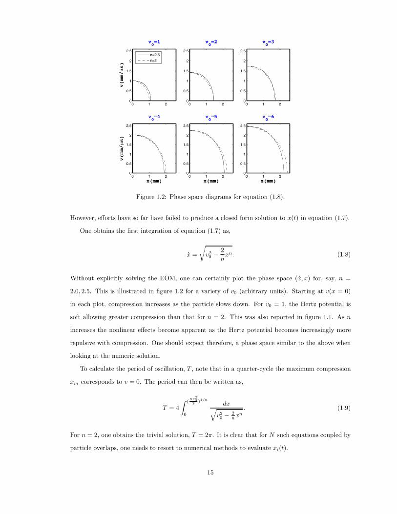
However, e!orts have so far have failed to produce a closed form solution to x(t) in equation (1.7).

One obtains the first integration of equation (1.7) as,

x =,

v20 $ 2

nxn. (1.8)

Without explicitly solving the EOM, one can certainly plot the phase space (x, x) for, say, n =

2.0, 2.5. This is illustrated in figure 1.2 for a variety of v0 (arbitrary units). Starting at v(x = 0)

in each plot, compression increases as the particle slows down. For v0 = 1, the Hertz potential is

soft allowing greater compression than that for n = 2. This was also reported in figure 1.1. As n

increases the nonlinear e!ects become apparent as the Hertz potential becomes increasingly more

repulsive with compression. One should expect therefore, a phase space similar to the above when

looking at the numeric solution.

To calculate the period of oscillation, T , note that in a quarter-cycle the maximum compression

xm corresponds to v = 0. The period can then be written as,

T = 4- (

nv20

2 )1/n

0

dx.v20 $ 2

nxn. (1.9)

For n = 2, one obtains the trivial solution, T = 2). It is clear that for N such equations coupled by

particle overlaps, one needs to resort to numerical methods to evaluate xi(t).

15

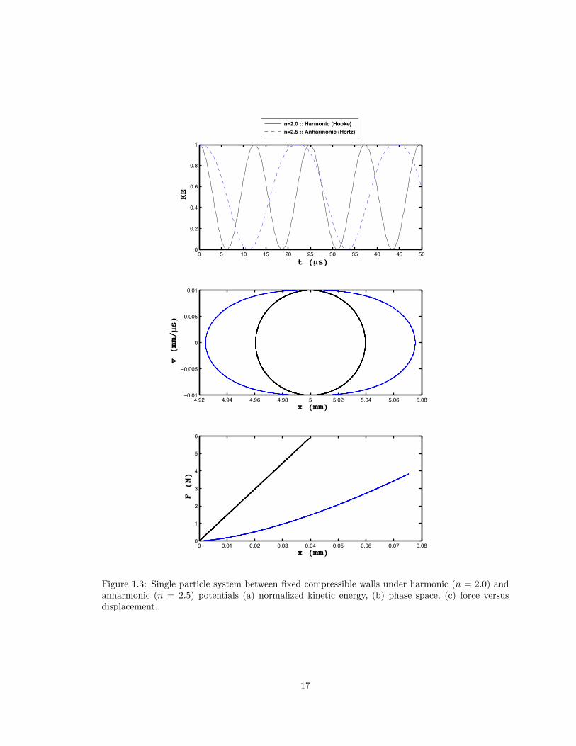
Figure 1.3 highlights the numeric results for the harmonic-like, n = 2 and Hertz, n = 2.5, cases.

Both are oscillators and what stands out immediately is the “softness” of the n = 2.5 potential.

This is visible both in panels (a)—where in the anharmonic case the period is longer—and (b)

where the closed trajectories in the anharmonic case clearly reach larger displacements in x. Panel

(c) demonstrates the relative strengths of F as a function of the displacement. It also appears

that the initial velocity, vi = 10m/s does not cause a compression significant enough for the Hertz

potential to become stronger than a quadratic. As such the sphere always behaves as a soft particle

whose softness increases with n. Note that these results are consistent with expectations from figure

1.2 where v0 = 1.

One can perform a quick study on a single particle in an overlap potential well, !n. In this

particular case, a soft particle—barely touching the boundaries—has an initial velocity, vi. One

can ask various questions such as how does the period of oscillation scale with n and vi? More

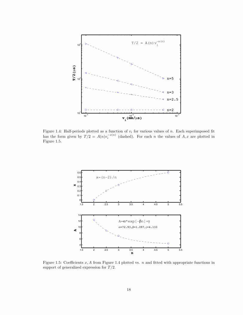
importantly, is it possible to obtain a single expression that evaluates T = T (n, vi)? Figure 1.4

shows the decay in period for increasing vi as well as the relative increase with n. The latter should

be expected since the “hardness” of the potential is proportional to n. Because of the excellent fit

a!orded by a power law, it is suspected that a single formula can describe the solution space. As

such we write,

T (n, vi) = A(n)v!x(n)i , (1.10)

where A(n), x(n) can be fit by some yet-to-be-determined function. It turns out that vi decays

as simply, (n $ 2)/n while the values comprising A decay exponentially with a single phase * and

plateau at +. These conclusions, including the fitting functions and associated coe"cients are plotted

in figure 1.5. This then allows us to write the period of a particle oscillating in an overlap potential

of exponent n with initial velocity vi as,

T/2 =/&e!!n + +

0v!(n!2)/n

i (1.11)

where the coe"cients are identified in the figures and for n = 5/2, T " v!1/5.

1.4.2 Two-Particle System

Figure 1.6 illustrates the velocity and position phase spaces of the binary system for the first 120 µs.

Several points of interest are identified in the velocity phase space—along with their corresponding

location in position space—and represent either a zero crossing or occasional extremum. Figure

16

0 ( 10 1( 20 2( +0 +( 40 4( (00

0"2

0"4

0"%

0"&

1

t (µs)

KE

n=2.0 :: Harmonic (Hooke) n=2.5 :: Anharmonic (Hertz)

4",2 4",4 4",% 4",& ( ("02 ("04 ("0% ("0&!0"01

!0"00(

0

0"00(

0"01

x (mm)

v (mm/µs)

0 0"01 0"02 0"0+ 0"04 0"0( 0"0% 0"0- 0"0&0

1

2

+

4

(

%

x (mm)

F (N)

Figure 1.3: Single particle system between fixed compressible walls under harmonic (n = 2.0) andanharmonic (n = 2.5) potentials (a) normalized kinetic energy, (b) phase space, (c) force versusdisplacement.

17

10!4 10!+ 10!2101

102

10+

vi(mm/µs)

T/2(µs)

n=2

n=2.5

n=3

n=5

T/2 = A(n)vi

−x(n)

Figure 1.4: Half-periods plotted as a function of vi for various values of n. Each superimposed fithas the form given by T/2 = A(n)v!x(n)

i (dashed). For each n the values of A, x are plotted inFigure 1.5.

1"( 2 2"( + +"( 4 4"( ( ("(

0

0"1

0"2

0"+

0"4

0"(

0"%

x=(n−2)/n

i

x

1"( 2 2"( + +"( 4 4"( ( ("(

4

%

&

10

12

14

A=!*exp[−"n]+#

!=72.93,"=1.097,#=4.133

n

A

Figure 1.5: Coe"cients x, A from Figure 1.4 plotted vs. n and fitted with appropriate functions insupport of generalized expression for T/2.

18

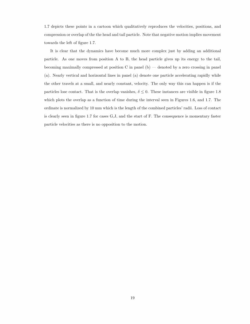
1.7 depicts these points in a cartoon which qualitatively reproduces the velocities, positions, and

compression or overlap of the the head and tail particle. Note that negative motion implies movement

towards the left of figure 1.7.

It is clear that the dynamics have become much more complex just by adding an additional

particle. As one moves from position A to B, the head particle gives up its energy to the tail,

becoming maximally compressed at position C in panel (b) — denoted by a zero crossing in panel

(a). Nearly vertical and horizontal lines in panel (a) denote one particle accelerating rapidly while

the other travels at a small, and nearly constant, velocity. The only way this can happen is if the

particles lose contact. That is the overlap vanishes, ! ( 0. These instances are visible in figure 1.8

which plots the overlap as a function of time during the interval seen in Figures 1.6, and 1.7. The

ordinate is normalized by 10 mm which is the length of the combined particles’ radii. Loss of contact

is clearly seen in figure 1.7 for cases G,J, and the start of F. The consequence is momentary faster

particle velocities as there is no opposition to the motion.

19

!0"01 !0"00& !0"00% !0"004 !0"002 0 0"002 0"004 0"00% 0"00& 0"01!0"01

!0"00&

!0"00%

!0"004

!0"002

0

0"002

0"004

0"00%

0"00&

0"01

vtail

vhead

A

B

C D

E

F

G

H

I

J

!0"0& !0"0% !0"04 !0"02 0 0"02 0"04 0"0% 0"0& 0"1 0"12!0"1

!0"0&

!0"0%

!0"04

!0"02

0

0"02

0"04

0"0%

0"0&

xtail

xhead A

BCD

E

F

G

H

I

J

Figure 1.6: Velocity and position phase diagrams for the two particle system. Dynamics are shownfor the first 120 µs with corresponding points of interest identified. Note that maximum velocitiesdo not necessarily correspond to crossing the t = 0 positions.

20

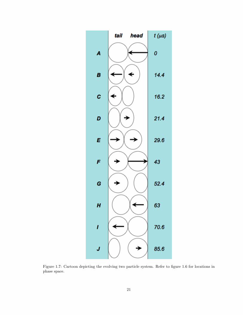
Figure 1.7: Cartoon depicting the evolving two particle system. Refer to figure 1.6 for locations inphase space.

21

0 20 40 %0 &0 100 1200

0"2

0"4

0"%

0"&

1

$

BC D E F G H I J

0 20 40 %0 &0 100 120

!0"1

!0"0(

0

0"0(

0"1

t (µs)

x (mm)

headtail

Figure 1.8: Overlap, !, as a function of time for the particle-particle interface in the N = 2 system.! is represented as a percentage of the two spheres combined radii since it is normalized by 10 mm(2Ri).

22

Chapter 2

The Simple Tapered Chain (STC)

2.1 Introduction

This chapter presents an in-depth and greatly extended study of TCs originally carried out by

Pfannes80. The results and sections of this chapter were reported by Doney and Sen25,26 and

presented at the 2005 American Physical Society’s topical meeting of shock compression in condensed

matter in Baltimore, MD. Specifically this work focuses on the ability to spread impulses out in time

and space rather than analyzing solitary wave propagation which is typically the dominating topic.

Section 2.2 addresses the hard-sphere approximation, with and without a term accounting for energy

loss at each collision. Section 2.3 looks at the numeric solution in terms of temporal behavior as

well as normalized kinetic energy (KE) and force parameter spaces. That section also includes a

discussion of how these systems partition energy. This is followed by a generalization of the systems’

characteristic fluctuations and the approach to a state referred to as quasi-equilibrium. The chapter

concludes with a mathematical fit to describe the normalized energy mitigation as a function of q,".

2.2 Hard-Sphere Approximation

Hard-sphere approximations di!er from the numerically simulated systems in two major ways. The

first is that, for the former, the chain is not bounded by fixed rigid walls. As a result, energy will not

continue to be transmitted up and down the chain. The second is that the potential becomes infinite

(n & ') and as a consequence, the energy packet is only 1 grain in width. The system therefore

propagates energy as independent collisions and is congruent to the model proposed by Wu121.

By generating an iterative form of the conservation equations, one can arrive at an expression for

the normalized kinetic energy (KE), EK = KEout/KEin. This ratio will be the primary variable

determining the absorptive quality of TCs.

The simple tapered chain (STC) is displayed in figure 2.1. To generate an initial disturbance, an

input velocity, vi, is applied to the rightmost and largest grain with radius ri. It propagates to the

23

0 10 20 +0 40 (0 %0 -0!10

!(

0

(

10

5is

tanc

e (m

m)

5istance (mm)

% vin

Figure 2.1: Simple tapered chain: N = 10, qs = 8%, L = 70.7 mm, ri = 5 mm. The rightmostparticle is grain i, its nearest neighbor is, i + 1, etc.

left, encountering an (initially) stationary grain of radius, ri+1. The radius of the (i + 1) particle

may be reduced to (1 $ q)ri. This tapering q will be constant along the entire length of the chain.

During the transmission of the impulse along the chain, there may be energy losses and we consider

two cases described in the following subsections.

2.2.1 Lossless STC Hard-Sphere Approximation

Ignoring any energy loss during a collision, we perform a STC hard-sphere approximation. Masses

and radii are expressed as

ri+1 = ri $ riqs = (1 $ qs)ri = $ri

mi = (Vi =43)r3

i ( = ,r3i (2.1)

mi+1 = ,r3i+1 = ,$3r3

i , (2.2)

where $ = 1 $ qs. Evaluating the conservation of momentum, with a single prime denoting post

collision values and the initial condition that the (i + 1) particle is stationary before a collision

(vi+1 = 0), all , cancel and we obtain

mivi + mi+1vi+1 = miv"i + mi+1v

"i+1

r3i vi = r3

i v"i + $3r3i v"i+1

vi = v"i + $3v"i+1, (2.3)

24

where equations (2.1, 2.2) have been used. Following the same procedure for the conservation of

energy while ignoring the factor of one-half yields,

v2i = v"2i + $3v"2i+1. (2.4)

Letting A = $3v"i+1 we can rewrite equation (2.3) in terms of v"i and substitute the resulting expression

into equation (2.4),

v2i = (vi $ A)2 + Av"i+1

= v2i $ 2Avi + A2 + Av"i+1

2vi = A + v"i+1

v"i+1

vi=

21 + $3

. (2.5)

Note that for one collision

KEout

KEin=

KE"i+1

KEi=

mi+1

mi

1v"i+1

vi

22

= $31

v"i+1

vi

22

∴ KE"i+1

KEi=

4$3

(1 + $3)2. (2.6)

For N particles there will be N $ 1 collisions, each of which have the ratio in equation (2.6).

Therefore, the normalized KE, EK , for the lossless STC hard-sphere approximation is given as

EK =

"4[1 $ q]3

(1 + [1 $ q]3)2

%N!1

. (2.7)

2.2.2 Lossy STC Hard-Sphere Approximation

The same approximation can be performed with some amount of energy loss, EL, per collision.

Consequently, the momentum equation (2.3) is unchanged, but equation (2.4) becomes

v2i = v"2i + $3v"2i+1 + EL. (2.8)

25

One then obtains a more complicated expression replacing equation (2.5):

v"i+1

vi=

2 $ EL"3viv!

i+1

1 + $3. (2.9)

We can make the substitution, EL " viv"i+1 or EL = ELviv"i+1, where EL is the constant of

proportionality. This adjustment yields

v"i+1

vi=

2$3 $ EL

$3(1 + $3).

The corresponding result for the normalized KE for N particles is

EK =

" 32(1 $ q)3 $ EL

42

(1 $ q)331 + (1 $ q)3

42

%N!1

. (2.10)

In the limit EL = 0, equation (2.10) reduces to the lossless case, equation (2.7), as one would expect.

Note that results are independent of initial velocity and size of the grains.

2.2.3 KE Parameter Space for STC Hard-Spheres

Figure 2.2 highlights the behavior of equation (2.10) for 0 ( q ( 0.1, 3 ( N ( 20 and selected EL.

Results indicate a greatly decreasing output of energy for modest values of EL. The decay of N also

takes on an exponential decay. Behavior of the tapering, q, resembles sigmoidal or gaussian decay

and approaches linear behavior with decreasing N . This can be seen in equations (2.7) and (2.10)

and is expected since for N = 1 there are no collisions and q becomes meaningless (it is defined for

a particle and its neighbor).

Interestingly, if the initial velocity is supplied to the smaller end of the TC, one also observes

shock absorption similar to the system in figure 1, albeit with less e"ciency. In this case, subsequent

particles are growing in size, i.e., ri+1 = (1 + q)ri. Equations (2.7) and (2.10) are modified accord-

ingly, and the result for a lossless system is illustrated in figure 2.3. Apparently, both configurations

mitigate a propagating pulse. Note that the range of axes in the figures are di!erent.

2.3 Numeric Solution

Simulations were performed for 3 ( N ( 20 and 0 ( q, " ( 0.1.

26

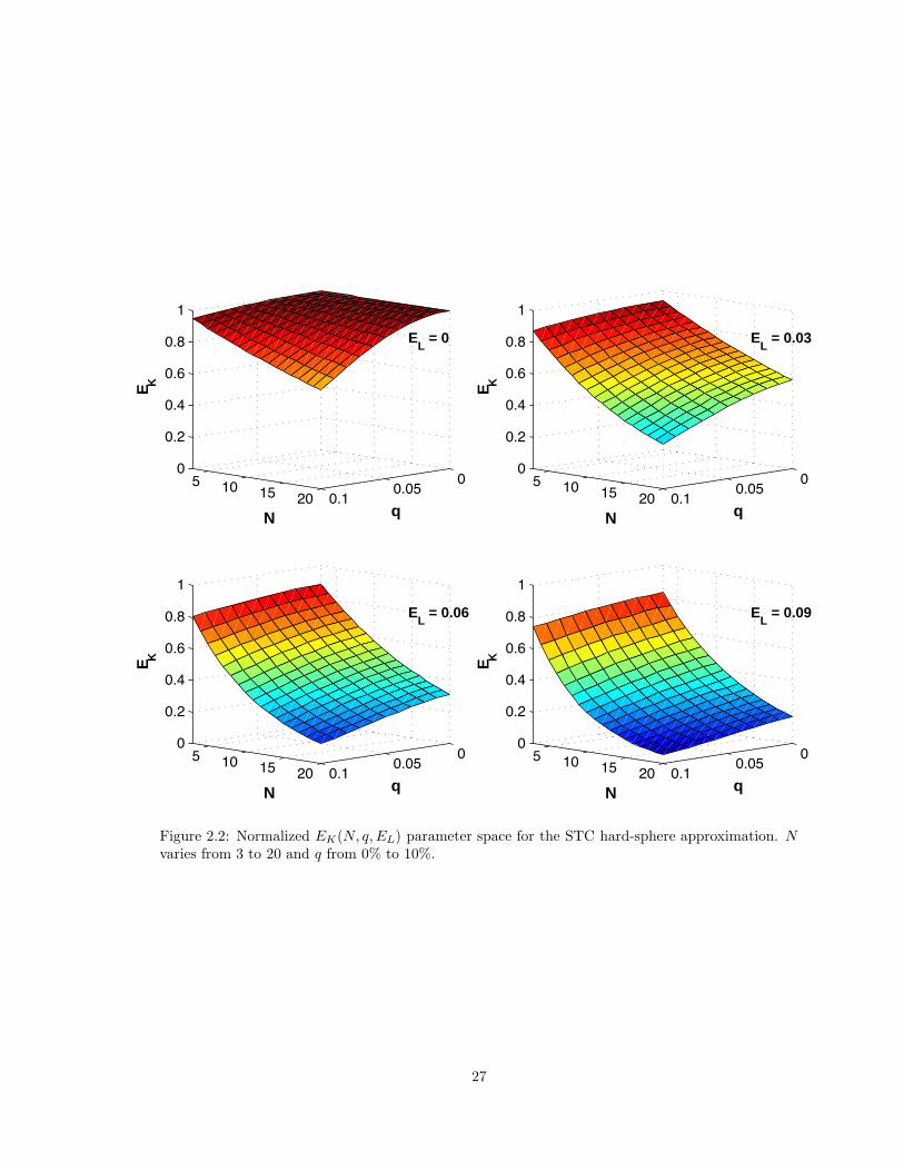
00"0(0"1

( 10 1( 20

0

0"2

0"4

0"%

0"&

1

EL = 0

q N

EK

00"0(0"1

( 10 1( 20

0

0"2

0"4

0"%

0"&

1

EL = 0.03

q N

EK

00"0(0"1

( 10 1( 20

0

0"2

0"4

0"%

0"&

1

EL = 0.06

q N

EK

00"0(0"1

( 10 1( 20

0

0"2

0"4

0"%

0"&

1

EL = 0.09

q N

EK

Figure 2.2: Normalized EK(N, q, EL) parameter space for the STC hard-sphere approximation. Nvaries from 3 to 20 and q from 0% to 10%.

27

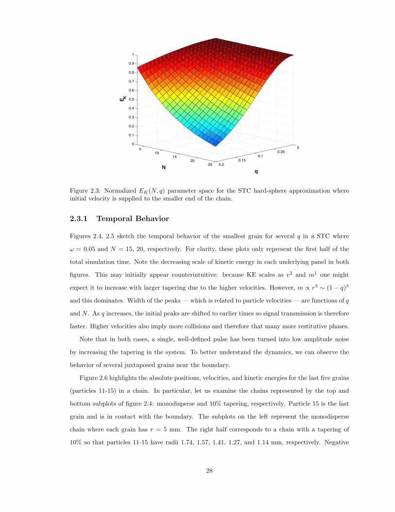
00"0(

0"10"1(

0"2

(10

1(20

2(

0

0"1

0"2

0"+

0"4

0"(

0"%

0"-

0"&

0",

1

q N

EK

Figure 2.3: Normalized EK(N, q) parameter space for the STC hard-sphere approximation whereinitial velocity is supplied to the smaller end of the chain.

2.3.1 Temporal Behavior

Figures 2.4, 2.5 sketch the temporal behavior of the smallest grain for several q in a STC where

" = 0.05 and N = 15, 20, respectively. For clarity, these plots only represent the first half of the

total simulation time. Note the decreasing scale of kinetic energy in each underlying panel in both

figures. This may initially appear counterintuitive: because KE scales as v2 and m1 one might

expect it to increase with larger tapering due to the higher velocities. However, m " r3 * (1 $ q)3

and this dominates. Width of the peaks — which is related to particle velocities — are functions of q

and N . As q increases, the initial peaks are shifted to earlier times so signal transmission is therefore

faster. Higher velocities also imply more collisions and therefore that many more restitutive phases.

Note that in both cases, a single, well-defined pulse has been turned into low amplitude noise

by increasing the tapering in the system. To better understand the dynamics, we can observe the

behavior of several juxtaposed grains near the boundary.

Figure 2.6 highlights the absolute positions, velocities, and kinetic energies for the last five grains

(particles 11-15) in a chain. In particular, let us examine the chains represented by the top and

bottom subplots of figure 2.4: monodisperse and 10% tapering, respectively. Particle 15 is the last

grain and is in contact with the boundary. The subplots on the left represent the monodisperse

chain where each grain has r = 5 mm. The right half corresponds to a chain with a tapering of

10% so that particles 11-15 have radii 1.74, 1.57, 1.41, 1.27, and 1.14 mm, respectively. Negative

28

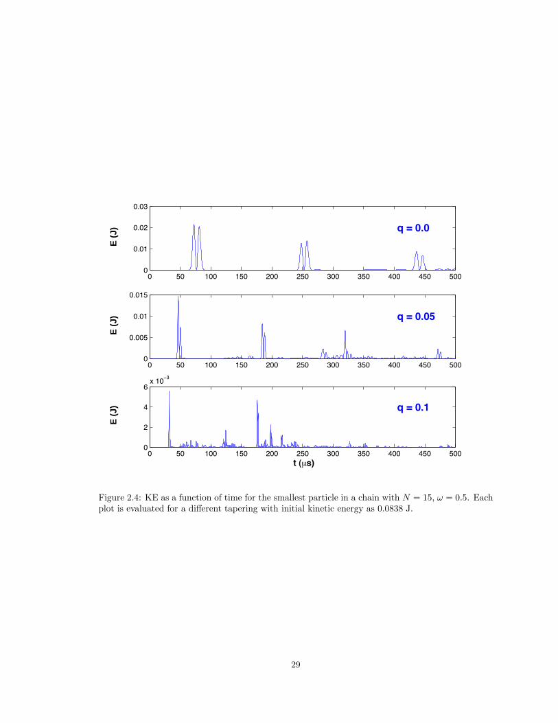
0 (0 100 1(0 200 2(0 +00 +(0 400 4(0 (000

0"01

0"02

0"0+

q = 0.0

E (

J)

0 (0 100 1(0 200 2(0 +00 +(0 400 4(0 (000

0"00(

0"01

0"01(

E (

J) q = 0.05

0 (0 100 1(0 200 2(0 +00 +(0 400 4(0 (000

2

4

%= 10!+

t (µs)

E (

J) q = 0.1

Figure 2.4: KE as a function of time for the smallest particle in a chain with N = 15, " = 0.5. Eachplot is evaluated for a di!erent tapering with initial kinetic energy as 0.0838 J.

29

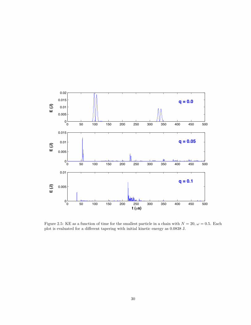
0 (0 100 1(0 200 2(0 +00 +(0 400 4(0 (000

0"00(

0"01

0"01(

0"02

q = 0.0

E (

J)

0 (0 100 1(0 200 2(0 +00 +(0 400 4(0 (000

0"00(

0"01

0"01(

q = 0.05

E (

J)

0 (0 100 1(0 200 2(0 +00 +(0 400 4(0 (000

0"00(

0"01

t (µs)

q = 0.1

E (

J)

Figure 2.5: KE as a function of time for the smallest particle in a chain with N = 20, " = 0.5. Eachplot is evaluated for a di!erent tapering with initial kinetic energy as 0.0838 J.

30

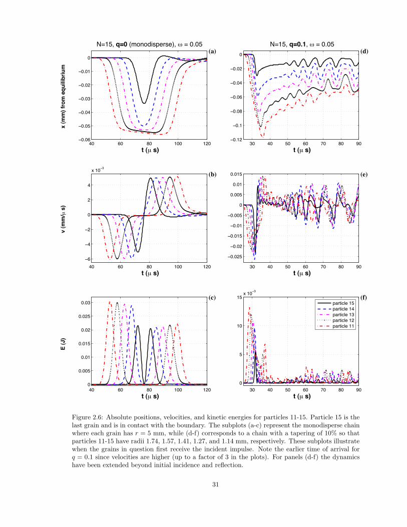
40 %0 &0 100 120!0"0%

!0"0(

!0"04

!0"0+

!0"02

!0"01

0

t (µ s)

x (m

m) f

rom

equ

ilibr

ium

>*1(? q=0 (monodisAerse)? & * 0"0( (a)

+0 40 (0 %0 -0 &0 ,0!0"12

!0"1

!0"0&

!0"0%

!0"04

!0"02

0

t (µ s)

>*1(? q=0.1? & * 0"0( (d)

40 %0 &0 100 120!%

!4

!2

0

2

4

= 10!+

t (µ s)

v (m

m/µ

s)

(b)

+0 40 (0 %0 -0 &0 ,0

!0"02(

!0"02

!0"01(

!0"01

!0"00(

0

0"00(

0"01

0"01(

t (µ s)

(e)

40 %0 &0 100 1200

0"00(

0"01

0"01(

0"02

0"02(

0"0+

t (µ s)

E (J

)

(c)

+0 40 (0 %0 -0 &0 ,00

(

10

1(= 10!+

t (µ s)

(f)Aarticle 1(Aarticle 14Aarticle 1+Aarticle 12Aarticle 11

Figure 2.6: Absolute positions, velocities, and kinetic energies for particles 11-15. Particle 15 is thelast grain and is in contact with the boundary. The subplots (a-c) represent the monodisperse chainwhere each grain has r = 5 mm, while (d-f) corresponds to a chain with a tapering of 10% so thatparticles 11-15 have radii 1.74, 1.57, 1.41, 1.27, and 1.14 mm, respectively. These subplots illustratewhen the grains in question first receive the incident impulse. Note the earlier time of arrival forq = 0.1 since velocities are higher (up to a factor of 3 in the plots). For panels (d-f) the dynamicshave been extended beyond initial incidence and reflection.

31

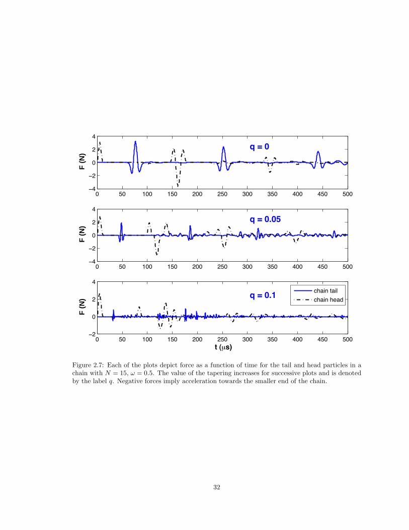
0 (0 100 1(0 200 2(0 +00 +(0 400 4(0 (00!4

!2

0

2

4

q = 0

F (

N)

0 (0 100 1(0 200 2(0 +00 +(0 400 4(0 (00!4

!2

0

2

4

q = 0.05

F (

N)

0 (0 100 1(0 200 2(0 +00 +(0 400 4(0 (00!2

0

2

4

q = 0.1

F (

N)

t (µs)

chain tailchain head

Figure 2.7: Each of the plots depict force as a function of time for the tail and head particles in achain with N = 15, " = 0.5. The value of the tapering increases for successive plots and is denotedby the label q. Negative forces imply acceleration towards the smaller end of the chain.

32

velocities and displacement imply motion towards the end of the chain.

For the monodisperse chain, the last five particles first receive and reflect the propagating impulse

between 40-120 µs. It also appears that for the monodisperse chain, there is about 5 µs of compression

for a given grain before it noticeably responds to the contact force and accelerates away. Observe

particle 11 acting upon particle 12 in panel (b) for example. Note that after another 5 µs particle

11 hits its peak velocity which is just about the time particle 13 starts to respond to the impulse.

When looking at the peak KE of particle 13 occuring at 62.5 µs, energy is primarily shared

among its two nearest neighbors such that most of the kinetic energy of the system is shared among

3 adjacent particles. The actual number, while still contested, is closer to 5 or 7, since there is a

small, but measurable amount of energy in the next layer of nearest neighbors. This is true for any

interior particle and is in agreement with Manciu, et. al.59,60. These solitary waves (SW) — the

“envelope” of the five grains in question — represent localized energy that maintain their width yet

decrease in amplitude after colliding with a boundary. The decrease of the tail particle’s velocity is

a result of the modified potential at the boundary.

At approximately 77 µs, nearly all energy is briefly stored as elastic potential energy. Simulta-

neously, particles 14 and 15 are maximally displaced from their equilibrium position while particles

11-13 are still slowly compressing towards the boundary. A close examination about this time shows

that the fourteenth grain is the first particle to reverse direction due to the restoring force of the

last particle. Acceleration plots indicate more clearly that this happens while the tail particle is still

being compressed with the boundary.

The big picture of energy propagation then consists of several regimes. In the microscopic sense

one could describe the elastic waves emanating from the contact region and reflecting within any

particular grain. Mesoscopic features have been the current focus of these plots and observations —

that is, bulk motion of a grain. And the macroscopic picture would be the solitary (longitudinal)

wave formed by several grains and discussed in previous work.

For the highly tapered chain (q = 0.1) on the right hand side of Figure 2.6, the last five particles

first receive and reflect the propagating impulse in about half the time as the monodisperse case. As

particles 11-14 are accelerated towards the end, their maximum speed increases due to their smaller

masses. Particle 11 accelerates at about 25 µs and compresses particle 12 for nearly 2 µs before it

starts to move. Shortly thereafter, particle 11 slows down at about 28 µs due to the contact force

with its neighbor, particle 12, and additional contact forces with particles 13-15. This is also true

for down range particles 12 and 13; however, the accelerations (not pictured) are enhanced as one

moves closer to the boundary.

33

What stands out dramatically in panel (f) is the absence of complete energy transmission. All

particles shown have a measurable amount of energy when the tail particle rebounds at about 32.5 µs

which is absent in the monodisperse chain. The displacement plot shows all grains biased towards

the tail of the chain from the equilibrium position. Each minima corresponds to a maximum in

their elastic potential energy. Because these occur at slightly skewed times, subsequent collision-

compression oscillations occur which are much more visible in the following 50 µs (not pictured). It

is di"cult to draw many conclusions from such a complicated landscape. However, it is expected

that no solitary wave is present in such chains: the dispersion due to tapering is too great.

When one records the force or energy at the end of the tapered chain with a sensor of some

sort, the patterns recorded vary for N and q as these plots suggest. As the tapering increases, the

pattern changes from a well-defined and periodic pulse to noise. This trend is visible for increasing

q in Figures 2.4, 2.5 and represents the thermalization that we are looking to exploit in various

applications.

2.3.2 KE and F Parameter Space Behavior

The e!ectiveness of TCs can be measured based on the normalized kinetic energy EK and force

surfaces formed by varying N , q, and ", thereby creating many tapered chain configurations. Specif-

ically, we form the ratio, EK = KEout/KEin, where KEout is the first peak felt by the last grain

and KEin is unchanged. Analogously, Fout is the first minimum felt by the last grain since the

direction of a negative force is into the wall or force sensor. The algorithm to pick out the first

turning point for each of these is straightforward. Since KE(t) is a column vector, one can iterate

through each element until the first occurence of (i + 1) < i is true. In that case, i represents the

peak. For force we compare against (i + 1) > i. Actually, normalization is a critical component in

determining the e!ectiveness of TCs and has been given a more thorough discussion in Appendix E.

Figure 2.8 highlights the numerical results for KE(N, q, constant "). The gaussian and exponen-

tial dependence on q and N , respectively stand out immediately. These KE surfaces represent STC

chains that thermalize more than half the incident energy introduced into the system. For example,

the least e!ective shock mitigating geometry that we’ve simulated here reduces the output kinetic

energy to approximately 40% of the input which is shown in panel (a) where N = 3, q = 0. The

“missing” energy is distributed among the other grains as kinetic and potential. Note that results

are independent of initial grain size. For monodisperse chains (q = 0), there is asymptotic behavior

as N increases. That is, when " = 0 for monodisperse chains, KE becomes a constant. This result

34

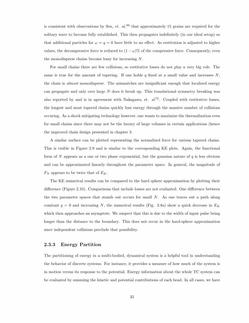
is consistent with observations by Sen, et. al.96 that approximately 15 grains are required for the

solitary wave to become fully established. This then propagates indefinitely (in our ideal setup) so

that additional particles for " = q = 0 have little to no e!ect. As restitution is adjusted to higher

values, the decompressive force is reduced to (1$")% of the compressive force. Consequently, even

the monodisperse chains become lossy for increasing N .

For small chains there are few collisions, so restitutive losses do not play a very big role. The

same is true for the amount of tapering. If one holds q fixed at a small value and increases N ,

the chain is almost monodisperse. The mismatches are insignificant enough that localized energy

can propagate and only over large N does it break up. This translational symmetry breaking was

also reported by and is in agreement with Nakagawa, et. al72. Coupled with restitutive losses,

the longest and most tapered chains quickly lose energy through the massive number of collisions

occuring. As a shock mitigating technology however, one wants to maximize the thermalization even

for small chains since there may not be the luxury of large volumes in certain applications (hence

the improved chain design presented in chapter 3.

A similar surface can be plotted representing the normalized force for various tapered chains.

This is visible in Figure 2.9 and is similar to the corresponding KE plots. Again, the functional

form of N appears as a one or two phase exponential, but the gaussian nature of q is less obvious

and can be approximated linearly throughout the parameter space. In general, the magnitude of

FN appears to be twice that of EK .

The KE numerical results can be compared to the hard sphere approximation by plotting their

di!erence (Figure 2.10). Comparisons that include losses are not evaluated. One di!erence between

the two parameter spaces that stands out occurs for small N . As one traces out a path along

constant q = 0 and increasing N , the numerical results (Fig. 2.8a) show a quick decrease in EK

which then approaches an asymptote. We suspect that this is due to the width of input pulse being

longer than the distance to the boundary. This does not occur in the hard-sphere approximation

since independent collisions preclude that possibility.

2.3.3 Energy Partition

The partitioning of energy in a multi-bodied, dynamical system is a helpful tool in understanding

the behavior of discrete systems. For instance, it provides a measure of how much of the system is

in motion versus its response to the potential. Energy information about the whole TC system can

be evaluated by summing the kinetic and potential contributions of each bead. In all cases, we have

35

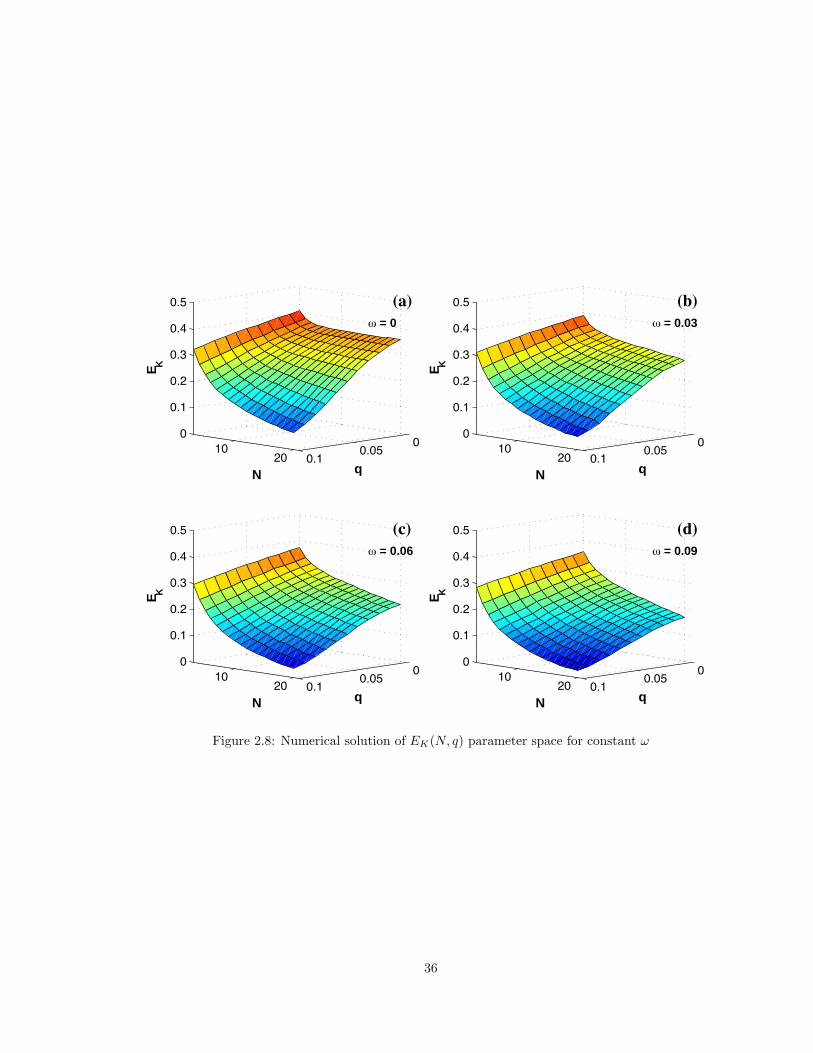
00"0(0"1

1020

0

0"1

0"2

0"+

0"4

0"( (a) & = 0

q N

EK

00"0(0"1

1020

0

0"1

0"2

0"+

0"4

0"( (b) & = 0.03

q N

EK

00"0(0"1

1020

0

0"1

0"2

0"+

0"4

0"( (c) & = 0.06

q N

EK

00"0(0"1

1020

0

0"1

0"2

0"+

0"4

0"( (d) & = 0.09

q N

EK

Figure 2.8: Numerical solution of EK(N, q) parameter space for constant "

36

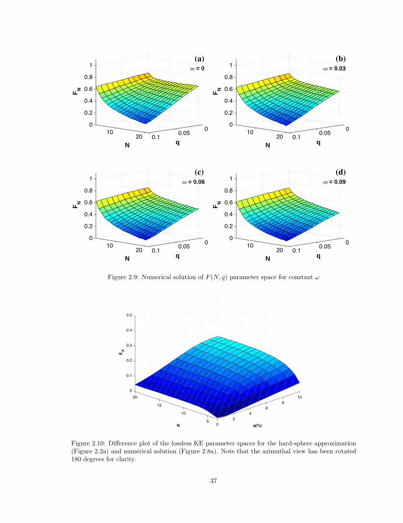
00"0(0"1

1020

0

0"2

0"4

0"%

0"&

1 (a)

& = 0

q N

FN

00"0(0"1

1020

0

0"2

0"4

0"%

0"&

1 (b)

& = 0.03

q N

FN

00"0(0"1

1020

0

0"2

0"4

0"%

0"&

1 (c)

& = 0.06

q N

FN

00"0(0"1

1020

0

0"2

0"4

0"%

0"&

1 (d)

& = 0.09

q N

FN

Figure 2.9: Numerical solution of F (N, q) parameter space for constant "

02

4%

&10

(

10

1(

200

0"1

0"2

0"+

0"4

0"(

q(%) N

E

K

Figure 2.10: Di!erence plot of the lossless KE parameter spaces for the hard-sphere approximation(Figure 2.2a) and numerical solution (Figure 2.8a). Note that the azimuthal view has been rotated180 degrees for clarity.

37

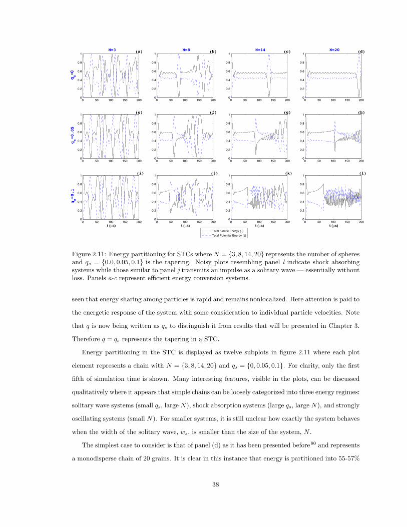
0 (0 100 1(0 2000

0"2

0"4

0"%

0"&

1

qs=0

N=3 (a)

Total Kinetic Energy (J)Total Iotential Energy (J)

0 (0 100 1(0 2000

0"2

0"4

0"%

0"&

1 N=8 (b)

0 (0 100 1(0 2000

0"2

0"4

0"%

0"&

1 N=14 (c)

0 (0 100 1(0 2000

0"2

0"4

0"%

0"&

1 N=20 (d)

0 (0 100 1(0 2000

0"2

0"4

0"%

0"&

1

qs=0.05

(e)

0 (0 100 1(0 2000

0"2

0"4

0"%

0"&

1 (f)

0 (0 100 1(0 2000

0"2

0"4

0"%

0"&

1 (g)

0 (0 100 1(0 2000

0"2

0"4

0"%

0"&

1 (h)

0 (0 100 1(0 2000

0"2

0"4

0"%

0"&

1

qs=0.1

t (µs)

(i)

0 (0 100 1(0 2000

0"2

0"4

0"%

0"&

1

t (µs)

(j)

0 (0 100 1(0 2000

0"2

0"4

0"%

0"&

1

t (µs)

(k)

0 (0 100 1(0 2000

0"2

0"4

0"%

0"&

1

t (µs)

(l)

Figure 2.11: Energy partitioning for STCs where N = {3, 8, 14, 20} represents the number of spheresand qs = {0.0, 0.05, 0.1} is the tapering. Noisy plots resembling panel l indicate shock absorbingsystems while those similar to panel j transmits an impulse as a solitary wave — essentially withoutloss. Panels a-c represent e"cient energy conversion systems.

seen that energy sharing among particles is rapid and remains nonlocalized. Here attention is paid to

the energetic response of the system with some consideration to individual particle velocities. Note

that q is now being written as qs to distinguish it from results that will be presented in Chapter 3.

Therefore q = qs represents the tapering in a STC.

Energy partitioning in the STC is displayed as twelve subplots in figure 2.11 where each plot

element represents a chain with N = {3, 8, 14, 20} and qs = {0, 0.05, 0.1}. For clarity, only the first

fifth of simulation time is shown. Many interesting features, visible in the plots, can be discussed

qualitatively where it appears that simple chains can be loosely categorized into three energy regimes:

solitary wave systems (small qs, large N), shock absorption systems (large qs, large N), and strongly

oscillating systems (small N). For smaller systems, it is still unclear how exactly the system behaves

when the width of the solitary wave, ws, is smaller than the size of the system, N .

The simplest case to consider is that of panel (d) as it has been presented before80 and represents

a monodisperse chain of 20 grains. It is clear in this instance that energy is partitioned into 55-57%

38

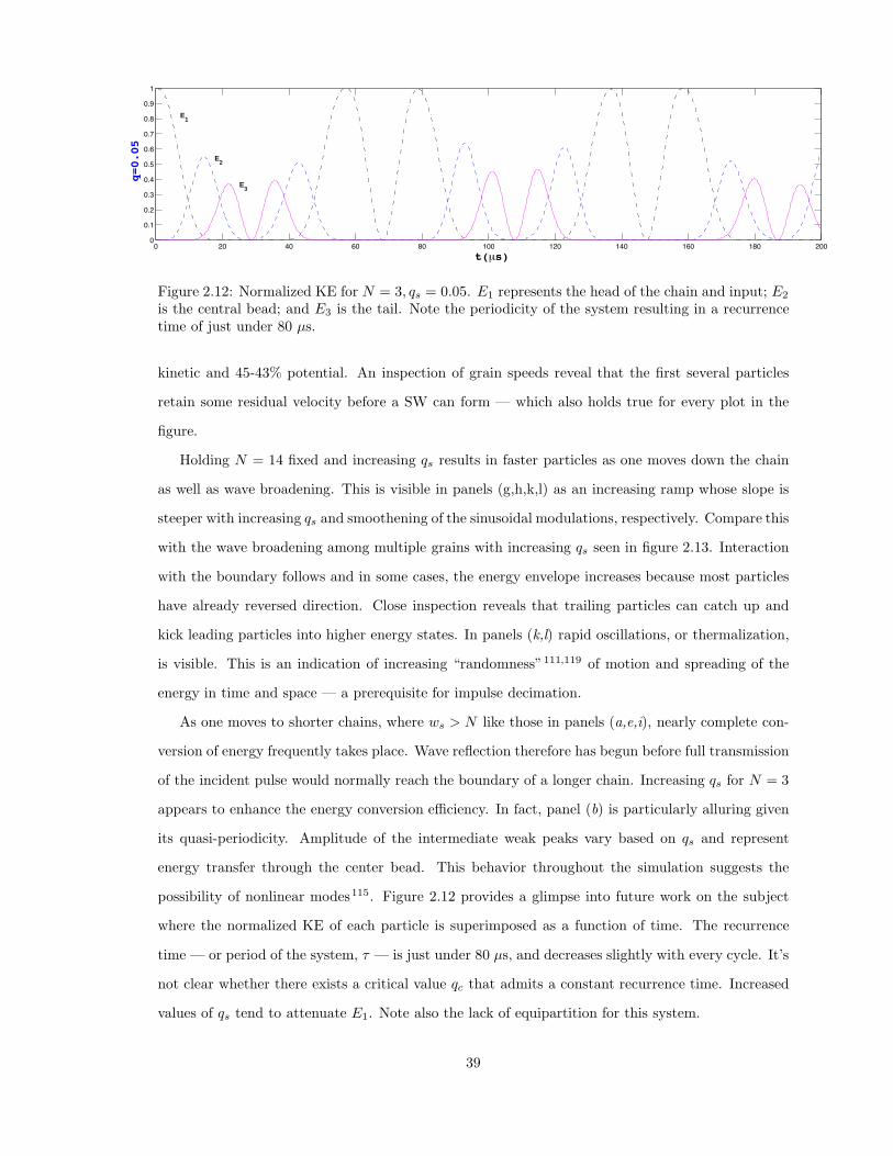
0 20 40 %0 &0 100 120 140 1%0 1&0 2000

0"1

0"2

0"+

0"4

0"(

0"%

0"-

0"&

0",

1

t(µs)

q=0.05

E1

E2

E3

Figure 2.12: Normalized KE for N = 3, qs = 0.05. E1 represents the head of the chain and input; E2

is the central bead; and E3 is the tail. Note the periodicity of the system resulting in a recurrencetime of just under 80 µs.

kinetic and 45-43% potential. An inspection of grain speeds reveal that the first several particles

retain some residual velocity before a SW can form — which also holds true for every plot in the

figure.

Holding N = 14 fixed and increasing qs results in faster particles as one moves down the chain

as well as wave broadening. This is visible in panels (g,h,k,l) as an increasing ramp whose slope is

steeper with increasing qs and smoothening of the sinusoidal modulations, respectively. Compare this

with the wave broadening among multiple grains with increasing qs seen in figure 2.13. Interaction

with the boundary follows and in some cases, the energy envelope increases because most particles

have already reversed direction. Close inspection reveals that trailing particles can catch up and

kick leading particles into higher energy states. In panels (k,l) rapid oscillations, or thermalization,

is visible. This is an indication of increasing “randomness”111,119 of motion and spreading of the

energy in time and space — a prerequisite for impulse decimation.

As one moves to shorter chains, where ws > N like those in panels (a,e,i), nearly complete con-

version of energy frequently takes place. Wave reflection therefore has begun before full transmission

of the incident pulse would normally reach the boundary of a longer chain. Increasing qs for N = 3

appears to enhance the energy conversion e"ciency. In fact, panel (b) is particularly alluring given

its quasi-periodicity. Amplitude of the intermediate weak peaks vary based on qs and represent

energy transfer through the center bead. This behavior throughout the simulation suggests the

possibility of nonlinear modes115. Figure 2.12 provides a glimpse into future work on the subject

where the normalized KE of each particle is superimposed as a function of time. The recurrence

time — or period of the system, ' — is just under 80 µs, and decreases slightly with every cycle. It’s

not clear whether there exists a critical value qc that admits a constant recurrence time. Increased

values of qs tend to attenuate E1. Note also the lack of equipartition for this system.

39

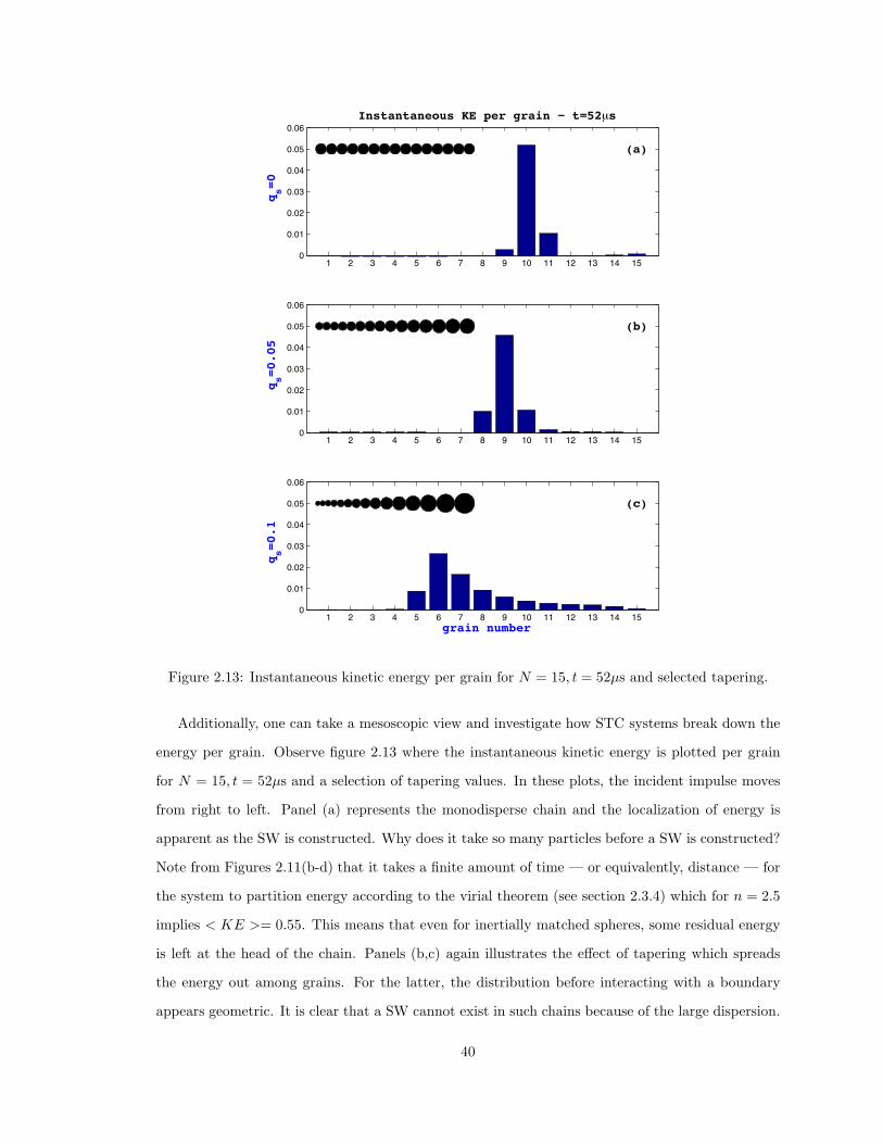
1 2 + 4 ( % - & , 10 11 12 1+ 14 1(0

0"01

0"02

0"0+

0"04

0"0(

0"0%

qs=0

Instantaneous KE per grain − t=52µs

(a)

1 2 + 4 ( % - & , 10 11 12 1+ 14 1(0

0"01

0"02

0"0+

0"04

0"0(

0"0%

qs=0.05

(b)

1 2 + 4 ( % - & , 10 11 12 1+ 14 1(0

0"01

0"02

0"0+

0"04

0"0(

0"0%

qs=0.1

grain number

(c)

Figure 2.13: Instantaneous kinetic energy per grain for N = 15, t = 52µs and selected tapering.

Additionally, one can take a mesoscopic view and investigate how STC systems break down the

energy per grain. Observe figure 2.13 where the instantaneous kinetic energy is plotted per grain

for N = 15, t = 52µs and a selection of tapering values. In these plots, the incident impulse moves

from right to left. Panel (a) represents the monodisperse chain and the localization of energy is

apparent as the SW is constructed. Why does it take so many particles before a SW is constructed?

Note from Figures 2.11(b-d) that it takes a finite amount of time — or equivalently, distance — for

the system to partition energy according to the virial theorem (see section 2.3.4) which for n = 2.5

implies < KE >= 0.55. This means that even for inertially matched spheres, some residual energy

is left at the head of the chain. Panels (b,c) again illustrates the e!ect of tapering which spreads

the energy out among grains. For the latter, the distribution before interacting with a boundary

appears geometric. It is clear that a SW cannot exist in such chains because of the large dispersion.

40

An even more illuminating series of images can be generated which shows the energy landscape

for all particles in the chain at all points in time. This is illustrated in figure 2.14. This series of plots

highlights the propagation of a pulse in time (horizontal axis) through the chain of grains (numbered

vertically) for several values of tapering, qs = {0, 0.02, 0.04, 0.06, 0.08, 0.1}. In each case, N = 20.

Kinetic energy is displayed and has been magnified several times in order to pick out the smaller

amplitude backscattering and wave phenomena. For the monodisperse chain, one can clearly see the

SW propagate, with negligible loss and backscattering for these early times. It is easy to see that

the SW velocity is approximately, 1 mm/µs, this is in contrast to the delta function impulse in grain

number 20 of 10 mm/µs — recall that some residual energy is left over in the first several grains.

This velocity decreases ever so slightly per cycle as the SW is destroyed and recreated imperfectly99

at the boundaries. As q increases, trapped energy is seen by the light horizontal bars in panels

(e,f) preceding 100 µs. What’s also very interesting to note here is the increasing magnitude of

backscattering during the return phase to particle 20. With increasing q, energy transfer is hindered

during the momentum transfer. Starting with panel (d) at 100 µs, many subsequent waves of lower

velocity towards the head of the chain are visible. At 500 µs, organized waves emerge that only

propagate through the smaller half of the chain (top half of panels). This e!ect also occurs for larger

q in panels (e,f) but more quickly — after the first interaction with the boundary. In these last

panels, the emergence of organized additional wave motion was unexpected.

2.3.4 The Approach to Quasi-equilibrium

What is the equilibrium state for a nonlinear system? For that matter, what is it for a strongly

nonlinear system with no restoring terms such as the Hertz potential? These questions have been

addressed by previous researchers with emphasis on FPU systems as discussed in section 1.2.2. Here

we outline an approach that leads to an interesting state referred to as quasi-equilibrium (qeq)

where the system exhibits some traits of being in equilbrium. It is found that (1) the eventual

state of the system appears to be initial condition dependent — this is opposite the expectation

of an equilibrium state; (2) the distribution of velocities of the system is roughly a gaussian - so

a maxwellian distribution of velocities is found — this is expected in an equlibrium phase; (3) TC

systems appear to have sustained fluctuations that deviate significantly from equilibrium.

41

Velocity Distributions

For a dilute gas in equilibrium, constituent particles exhibit a maxwellian (or gaussian) velocity

distribution84. One can therefore measure whether a similar system has reached equilibrium by

binning the velocities of each particle and observing whether the profile is that of a gaussian — as

figures 2.15, 2.16 do for N = 4, 20, respectively. In these panels, there are 50 bins ranging from

-0.01 to 0.01 mm/µs where the vertical axes represents the count per bin. Note that each panel

automatically adjusts the number of counts. In both cases, particle 1 represents the end of the chain

and particle N represents the head where the initial impulse was applied. In addition, simulation

time was extensive: 10 ms. For earlier times, the profiles di!ered markedly from a gaussian. The

plots show that with fewer particles, it is more common to find higher velocities, that is they don’t

decay significantly. For large N however, velocities decay to the point of a super-abundance near

the mean value — note the large increase of counts. It was expected that boundary particles would

stand-out in their profiles; however, interior and boundary particles appear indistinguishable in this

representation. Something that is missing from these plots is the temporal dependence — that is,

how long does it take to reach such profiles?

Equipartition

The next issue that can be addressed is whether or not one has equipartition of energy. The virial

theorem37,47,103 describes the average kinetic and potential energy in a system. If the force can be

derived from a potential of degree, n, then the virial theorem becomes,

12n < PE >=< KE >

< KE >=n

(n + 2)(2.11)

where the normalized total energy, E = 1 =< KE > + < PE >, has been used to eliminate

< PE >. This is the expected mean value of KE for the system. Note that n = 2 is the only case

where the energy is equally divided between potential and kinetic. Thus, is the strictest sense of the

word, equipartition has been achieved. One can compare results from the simulation to the these

expectations. Figure 2.17 illustrates the average KE as a function of N for several values of n. It

should not be surprising that < KE > is independent of N since it has no explicit dependence in

the Hamiltonian. Figure 2.23 demonstrates that the simulational results agree with what one would

expect from equation (2.11).

42

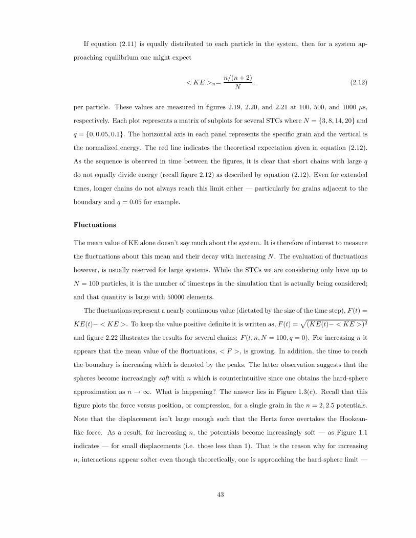
If equation (2.11) is equally distributed to each particle in the system, then for a system ap-

proaching equilibrium one might expect

< KE >n=n/(n + 2)

N, (2.12)

per particle. These values are measured in figures 2.19, 2.20, and 2.21 at 100, 500, and 1000 µs,

respectively. Each plot represents a matrix of subplots for several STCs where N = {3, 8, 14, 20} and

q = {0, 0.05, 0.1}. The horizontal axis in each panel represents the specific grain and the vertical is

the normalized energy. The red line indicates the theoretical expectation given in equation (2.12).

As the sequence is observed in time between the figures, it is clear that short chains with large q

do not equally divide energy (recall figure 2.12) as described by equation (2.12). Even for extended

times, longer chains do not always reach this limit either — particularly for grains adjacent to the

boundary and q = 0.05 for example.

Fluctuations

The mean value of KE alone doesn’t say much about the system. It is therefore of interest to measure

the fluctuations about this mean and their decay with increasing N . The evaluation of fluctuations

however, is usually reserved for large systems. While the STCs we are considering only have up to

N = 100 particles, it is the number of timesteps in the simulation that is actually being considered;

and that quantity is large with 50000 elements.

The fluctuations represent a nearly continuous value (dictated by the size of the time step), F (t) =

KE(t)$ < KE >. To keep the value positive definite it is written as, F (t) =!

(KE(t)$ < KE >)2

and figure 2.22 illustrates the results for several chains: F (t, n, N = 100, q = 0). For increasing n it

appears that the mean value of the fluctuations, < F >, is growing. In addition, the time to reach

the boundary is increasing which is denoted by the peaks. The latter observation suggests that the

spheres become increasingly soft with n which is counterintuitive since one obtains the hard-sphere

approximation as n & '. What is happening? The answer lies in Figure 1.3(c). Recall that this

figure plots the force versus position, or compression, for a single grain in the n = 2, 2.5 potentials.

Note that the displacement isn’t large enough such that the Hertz force overtakes the Hookean-

like force. As a result, for increasing n, the potentials become increasingly soft — as Figure 1.1

indicates — for small displacements (i.e. those less than 1). That is the reason why for increasing

n, interactions appear softer even though theoretically, one is approaching the hard-sphere limit —

43

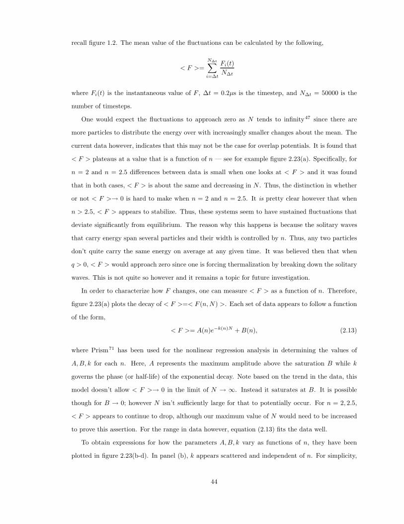
recall figure 1.2. The mean value of the fluctuations can be calculated by the following,

< F >=N∆t&

i=!t

Fi(t)N!t

where Fi(t) is the instantaneous value of F , #t = 0.2µs is the timestep, and N!t = 50000 is the

number of timesteps.

One would expect the fluctuations to approach zero as N tends to infinity47 since there are

more particles to distribute the energy over with increasingly smaller changes about the mean. The

current data however, indicates that this may not be the case for overlap potentials. It is found that

< F > plateaus at a value that is a function of n — see for example figure 2.23(a). Specifically, for

n = 2 and n = 2.5 di!erences between data is small when one looks at < F > and it was found

that in both cases, < F > is about the same and decreasing in N . Thus, the distinction in whether

or not < F >& 0 is hard to make when n = 2 and n = 2.5. It is pretty clear however that when

n > 2.5, < F > appears to stabilize. Thus, these systems seem to have sustained fluctuations that

deviate significantly from equilibrium. The reason why this happens is because the solitary waves

that carry energy span several particles and their width is controlled by n. Thus, any two particles

don’t quite carry the same energy on average at any given time. It was believed then that when

q > 0, < F > would approach zero since one is forcing thermalization by breaking down the solitary

waves. This is not quite so however and it remains a topic for future investigation.

In order to characterize how F changes, one can measure < F > as a function of n. Therefore,

figure 2.23(a) plots the decay of < F >=< F (n, N) >. Each set of data appears to follow a function

of the form,

< F >= A(n)e!k(n)N + B(n), (2.13)

where Prism71 has been used for the nonlinear regression analysis in determining the values of

A, B, k for each n. Here, A represents the maximum amplitude above the saturation B while k

governs the phase (or half-life) of the exponential decay. Note based on the trend in the data, this

model doesn’t allow < F >& 0 in the limit of N & '. Instead it saturates at B. It is possible

though for B & 0; however N isn’t su"ciently large for that to potentially occur. For n = 2, 2.5,

< F > appears to continue to drop, although our maximum value of N would need to be increased

to prove this assertion. For the range in data however, equation (2.13) fits the data well.

To obtain expressions for how the parameters A, B, k vary as functions of n, they have been

plotted in figure 2.23(b-d). In panel (b), k appears scattered and independent of n. For simplicity,

44

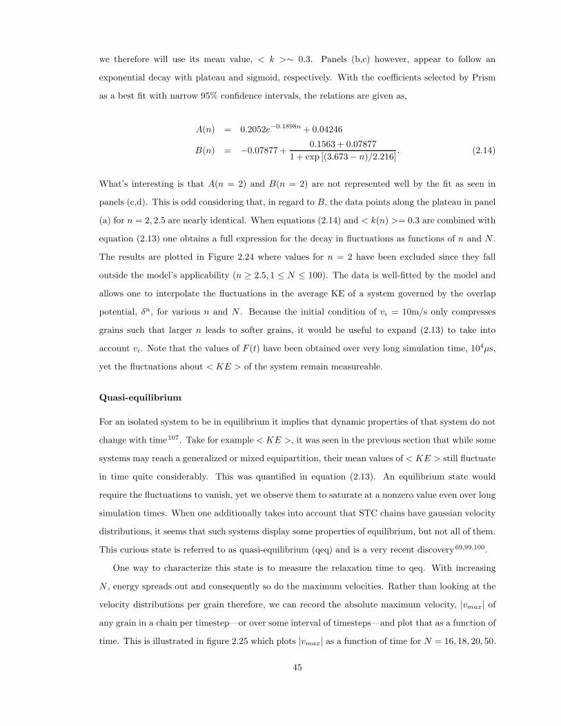
we therefore will use its mean value, < k >* 0.3. Panels (b,c) however, appear to follow an

exponential decay with plateau and sigmoid, respectively. With the coe"cients selected by Prism

as a best fit with narrow 95% confidence intervals, the relations are given as,

A(n) = 0.2052e!0.1898n + 0.04246

B(n) = $0.07877 +0.1563 + 0.07877

1 + exp [(3.673 $ n)/2.216]. (2.14)

What’s interesting is that A(n = 2) and B(n = 2) are not represented well by the fit as seen in

panels (c,d). This is odd considering that, in regard to B, the data points along the plateau in panel

(a) for n = 2, 2.5 are nearly identical. When equations (2.14) and < k(n) >= 0.3 are combined with

equation (2.13) one obtains a full expression for the decay in fluctuations as functions of n and N .

The results are plotted in Figure 2.24 where values for n = 2 have been excluded since they fall

outside the model’s applicability (n % 2.5, 1 ( N ( 100). The data is well-fitted by the model and

allows one to interpolate the fluctuations in the average KE of a system governed by the overlap

potential, !n, for various n and N . Because the initial condition of vi = 10m/s only compresses

grains such that larger n leads to softer grains, it would be useful to expand (2.13) to take into

account vi. Note that the values of F (t) have been obtained over very long simulation time, 104µs,

yet the fluctuations about < KE > of the system remain measureable.

Quasi-equilibrium

For an isolated system to be in equilibrium it implies that dynamic properties of that system do not

change with time107. Take for example < KE >, it was seen in the previous section that while some

systems may reach a generalized or mixed equipartition, their mean values of < KE > still fluctuate

in time quite considerably. This was quantified in equation (2.13). An equilibrium state would

require the fluctuations to vanish, yet we observe them to saturate at a nonzero value even over long

simulation times. When one additionally takes into account that STC chains have gaussian velocity

distributions, it seems that such systems display some properties of equilibrium, but not all of them.

This curious state is referred to as quasi-equilibrium (qeq) and is a very recent discovery69,99,100.

One way to characterize this state is to measure the relaxation time to qeq. With increasing

N , energy spreads out and consequently so do the maximum velocities. Rather than looking at the

velocity distributions per grain therefore, we can record the absolute maximum velocity, |vmax| of

any grain in a chain per timestep—or over some interval of timesteps—and plot that as a function of

time. This is illustrated in figure 2.25 which plots |vmax| as a function of time for N = 16, 18, 20, 50.

45

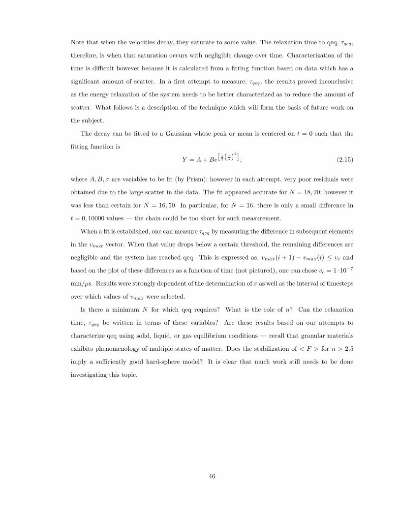
Note that when the velocities decay, they saturate to some value. The relaxation time to qeq, 'qeq ,

therefore, is when that saturation occurs with negligible change over time. Characterization of the

time is di"cult however because it is calculated from a fitting function based on data which has a

significant amount of scatter. In a first attempt to measure, 'qeq , the results proved inconclusive

as the energy relaxation of the system needs to be better characterized as to reduce the amount of

scatter. What follows is a description of the technique which will form the basis of future work on

the subject.

The decay can be fitted to a Gaussian whose peak or mean is centered on t = 0 such that the

fitting function is

Y = A + Be3

12

/tσ

024, (2.15)

where A, B,# are variables to be fit (by Prism); however in each attempt, very poor residuals were

obtained due to the large scatter in the data. The fit appeared accurate for N = 18, 20; however it

was less than certain for N = 16, 50. In particular, for N = 16, there is only a small di!erence in

t = 0, 10000 values — the chain could be too short for such measurement.

When a fit is established, one can measure 'qeq by measuring the di!erence in subsequent elements

in the vmax vector. When that value drops below a certain threshold, the remaining di!erences are

negligible and the system has reached qeq. This is expressed as, vmax(i + 1) $ vmax(i) ( vc and

based on the plot of these di!erences as a function of time (not pictured), one can chose vc = 1 ·10!7

mm/µs. Results were strongly dependent of the determination of # as well as the interval of timesteps

over which values of vmax were selected.

Is there a minimum N for which qeq requires? What is the role of n? Can the relaxation

time, 'qeq be written in terms of these variables? Are these results based on our attempts to

characterize qeq using solid, liquid, or gas equilibrium conditions — recall that granular materials

exhibits phenomenology of multiple states of matter. Does the stabilization of < F > for n > 2.5

imply a su"ciently good hard-sphere model? It is clear that much work still needs to be done

investigating this topic.

46

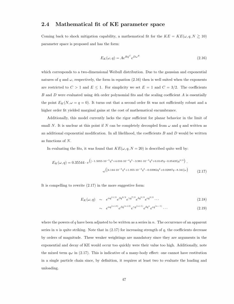
2.4 Mathematical fit of KE parameter space

Coming back to shock mitigation capability, a mathematical fit for the KE = KE(", q, N " 10)

parameter space is proposed and has the form:

EK(", q) = AeBqC

eD#E

(2.16)

which corresponds to a two-dimensional Weibull distribution. Due to the gaussian and exponential

natures of q and ", respectively, the form in equation (2.16) then is well suited when the exponents

are restricted to C > 1 and E ( 1. For simplicity we set E = 1 and C = 3/2. The coe"cients

B and D were evaluated using 4th order polynomial fits and the scaling coe"cient A is essentially

the point EK(N," = q = 0). It turns out that a second order fit was not su"ciently robust and a

higher order fit yielded marginal gains at the cost of mathematical encumbrance.

Additionally, this model currently lacks the rigor su"cient for planar behavior in the limit of

small N . It is unclear at this point if N can be completely decoupled from " and q and written as

an additional exponential modification. In all likelihood, the coe"cients B and D would be written

as functions of N .

In evaluating the fits, it was found that KE(", q, N = 20) is described quite well by:

EK(", q) = 0.35544 · e/[!1.5055·10"5q4+4.016·10"4q3!3.981·10"3q2+0.0147q!0.05435]q3/2

0·

·e/[4.144·10"5q4+1.955·10"3q3!0.03962q2+0.02887q!8.341]#

0(2.17)

It is compelling to rewrite (2.17) in the more suggestive form:

EK(", q) * e$q11/2e!q9/2

e%q7/2e&q

5/2e"q

3/2· · · (2.18)

* e$q(n+3)e!q(n+2)

e%q(n+1)e&q

n

e"q(n"1)

· · · (2.19)

where the powers of q have been adjusted to be written as a series in n. The occurrence of an apparent

series in n is quite striking. Note that in (2.17) for increasing strength of q, the coe"cients decrease

by orders of magnitude. These weaker weightings are mandatory since they are arguments in the

exponential and decay of KE would occur too quickly were their value too high. Additionally, note

the mixed term q" in (2.17). This is indicative of a many-body e!ect: one cannot have restitution

in a single particle chain since, by definition, it requires at least two to evaluate the loading and

unloading.

47

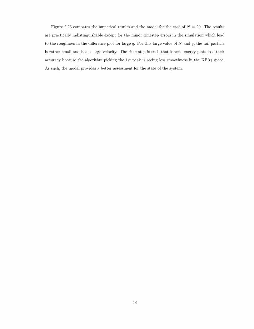
Figure 2.26 compares the numerical results and the model for the case of N = 20. The results

are practically indistinguishable except for the minor timestep errors in the simulation which lead

to the roughness in the di!erence plot for large q. For this large value of N and q, the tail particle

is rather small and has a large velocity. The time step is such that kinetic energy plots lose their

accuracy because the algorithm picking the 1st peak is seeing less smoothness in the KE(t) space.

As such, the model provides a better assessment for the state of the system.

48

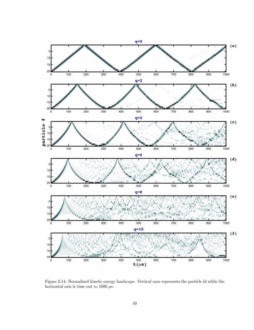
q=0(a)

0 100 200 +00 400 (00 %00 -00 &00 ,00 1000

(

10

1(

20

q=2(b)

0 100 200 +00 400 (00 %00 -00 &00 ,00 1000

(

10

1(

20

q=4(c)

particle #

0 100 200 +00 400 (00 %00 -00 &00 ,00 1000

(

10

1(

20

q=6(d)

0 100 200 +00 400 (00 %00 -00 &00 ,00 1000

(

10

1(

20

q=8(e)

0 100 200 +00 400 (00 %00 -00 &00 ,00 1000

(

10

1(

20

q=10(f)

t(µs)0 100 200 +00 400 (00 %00 -00 &00 ,00 1000

(

10

1(

20

Figure 2.14: Normalized kinetic energy landscape. Vertical axes represents the particle id while thehorizontal axis is time out to 1000 µs.

49

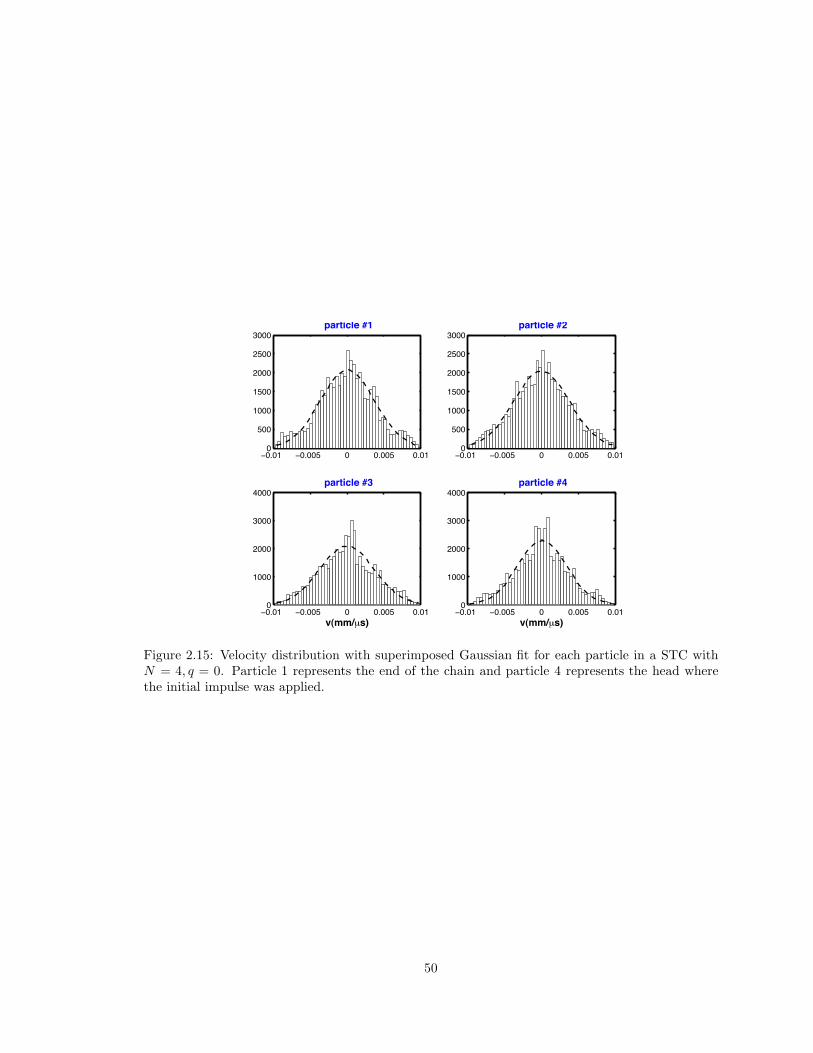
!0"01 !0"00( 0 0"00( 0"010

(00

1000

1(00

2000

2(00

+000 particle #1

!0"01 !0"00( 0 0"00( 0"010

(00

1000

1(00

2000

2(00

+000 particle #2

!0"01 !0"00( 0 0"00( 0"010

1000

2000

+000

4000 particle #3

v(mm/µs)!0"01 !0"00( 0 0"00( 0"01

0

1000

2000

+000

4000 particle #4

v(mm/µs)

Figure 2.15: Velocity distribution with superimposed Gaussian fit for each particle in a STC withN = 4, q = 0. Particle 1 represents the end of the chain and particle 4 represents the head wherethe initial impulse was applied.

50

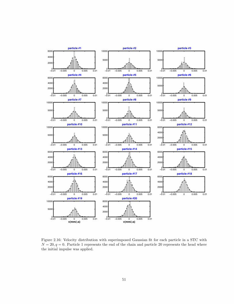
!0"01 !0"00( 0 0"00( 0"010

2000

4000

%000 particle #1

!0"01 !0"00( 0 0"00( 0"010

(000

10000 particle #2

!0"01 !0"00( 0 0"00( 0"010

(000

10000 particle #3

!0"01 !0"00( 0 0"00( 0"010

2000

4000

%000 particle #4

!0"01 !0"00( 0 0"00( 0"010

2000

4000

%000 particle #5

!0"01 !0"00( 0 0"00( 0"010

(000

10000 particle #6

!0"01 !0"00( 0 0"00( 0"010

(000

10000 particle #7

!0"01 !0"00( 0 0"00( 0"010

(000

10000 particle #8

!0"01 !0"00( 0 0"00( 0"010

(000

10000 particle #9

!0"01 !0"00( 0 0"00( 0"010

(000

10000 particle #10

!0"01 !0"00( 0 0"00( 0"010

(000

10000 particle #11

!0"01 !0"00( 0 0"00( 0"010

2000

4000

%000 particle #12

!0"01 !0"00( 0 0"00( 0"010

2000

4000

%000 particle #13

!0"01 !0"00( 0 0"00( 0"010

2000

4000

%000 particle #14

!0"01 !0"00( 0 0"00( 0"010

2000

4000

%000 particle #15

!0"01 !0"00( 0 0"00( 0"010

2000

4000

%000 particle #16

!0"01 !0"00( 0 0"00( 0"010

2000

4000

%000 particle #17

!0"01 !0"00( 0 0"00( 0"010

2000

4000

%000 particle #18

!0"01 !0"00( 0 0"00( 0"010

(000

10000 particle #19

v(mm/µs)!0"01 !0"00( 0 0"00( 0"01

0

2000

4000

%000 particle #20

v(mm/µs)

Figure 2.16: Velocity distribution with superimposed Gaussian fit for each particle in a STC withN = 20, q = 0. Particle 1 represents the end of the chain and particle 20 represents the head wherethe initial impulse was applied.

51

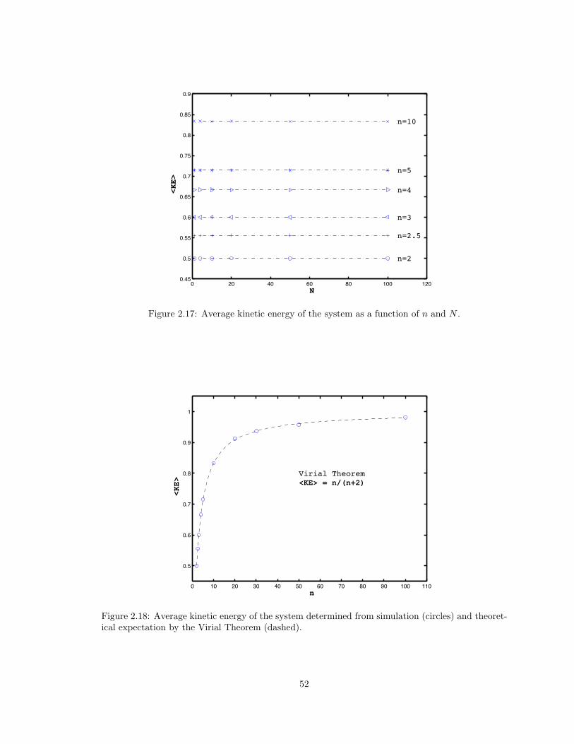
0 20 40 %0 &0 100 1200"4(

0"(

0"((

0"%

0"%(

0"-

0"-(

0"&

0"&(

0",

N

<KE>

n=2

n=2.5

n=3

n=4

n=5

n=10

Figure 2.17: Average kinetic energy of the system as a function of n and N .

0 10 20 +0 40 (0 %0 -0 &0 ,0 100 110

0"(

0"%

0"-

0"&

0",

1

n

<KE>

Virial Theorem<KE> = n/(n+2)

Figure 2.18: Average kinetic energy of the system determined from simulation (circles) and theoret-ical expectation by the Virial Theorem (dashed).

52

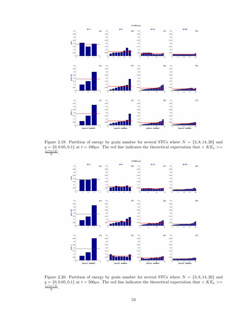
0 1 2 + 40

0"0(

0"1

0"1(

0"2

0"2(

0"+

0"+(

0"4

q=0

N=3(a)

0 2 4 % &0

0"0(

0"1

0"1(

0"2

0"2(

0"+

0"+(

0"4 N=8

(b)

0 ( 10 1(0

0"0(

0"1

0"1(

0"2

0"2(

0"+

0"+(

0"4 N=14

(c)

0 ( 10 1( 200

0"0(

0"1

0"1(

0"2

0"2(

0"+

0"+(

0"4 N=20

(d)

0 1 2 + 40

0"0(

0"1

0"1(

0"2

0"2(

0"+

0"+(

0"4

q=0.05

(e)

0 2 4 % &0

0"0(

0"1

0"1(

0"2

0"2(

0"+

0"+(

0"4 (f)

0 ( 10 1(0

0"0(

0"1

0"1(

0"2

0"2(

0"+

0"+(

0"4 (g)

0 ( 10 1( 200

0"0(

0"1

0"1(

0"2

0"2(

0"+

0"+(

0"4 (h)

0 1 2 + 40

0"0(

0"1

0"1(

0"2

0"2(

0"+

0"+(

0"4

grain number

q=0.1

(i)

0 2 4 % &0

0"0(

0"1

0"1(

0"2

0"2(

0"+

0"+(

0"4

grain number

(j)

0 ( 10 1(0

0"0(

0"1

0"1(

0"2

0"2(

0"+

0"+(

0"4

grain number

(k)

0 ( 10 1( 200

0"0(

0"1

0"1(

0"2

0"2(

0"+

0"+(

0"4

grain number

(l)

t=100(µs)

Figure 2.19: Partition of energy by grain number for several STCs where N = {3, 8, 14, 20} andq = {0, 0.05, 0.1} at t = 100µs. The red line indicates the theoretical expectation that < KEn >=n/(n+2)

N .

0 1 2 + 40

0"0(

0"1

0"1(

0"2

0"2(

0"+

0"+(

0"4

q=0

N=3(a)

0 2 4 % &0

0"0(

0"1

0"1(

0"2

0"2(

0"+

0"+(

0"4 N=8

(b)

0 ( 10 1(0

0"0(

0"1

0"1(

0"2

0"2(

0"+

0"+(

0"4 N=14

(c)

0 ( 10 1( 200

0"0(

0"1

0"1(

0"2

0"2(

0"+

0"+(

0"4 N=20

(d)

0 1 2 + 40

0"0(

0"1

0"1(

0"2

0"2(

0"+

0"+(

0"4

q=0.05

(e)

0 2 4 % &0

0"0(

0"1

0"1(

0"2

0"2(

0"+

0"+(

0"4 (f)

0 ( 10 1(0

0"0(

0"1

0"1(

0"2

0"2(

0"+

0"+(

0"4 (g)

0 ( 10 1( 200

0"0(

0"1

0"1(

0"2

0"2(

0"+

0"+(

0"4 (h)

0 1 2 + 40

0"0(

0"1

0"1(

0"2

0"2(

0"+

0"+(

0"4

grain number

q=0.1

(i)

0 2 4 % &0

0"0(

0"1

0"1(

0"2

0"2(

0"+

0"+(

0"4

grain number

(j)

0 ( 10 1(0

0"0(

0"1

0"1(

0"2

0"2(

0"+

0"+(

0"4

grain number

(k)

0 ( 10 1( 200

0"0(

0"1

0"1(

0"2

0"2(

0"+

0"+(

0"4

grain number

(l)

t=500(µs)


N .

53

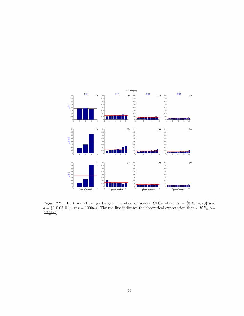
0 1 2 + 40

0"0(

0"1

0"1(

0"2

0"2(

0"+

0"+(

0"4

q=0

N=3(a)

0 2 4 % &0

0"0(

0"1

0"1(

0"2

0"2(

0"+

0"+(

0"4 N=8

(b)

0 ( 10 1(0

0"0(

0"1

0"1(

0"2

0"2(

0"+

0"+(

0"4 N=14

(c)

0 ( 10 1( 200

0"0(

0"1

0"1(

0"2

0"2(

0"+

0"+(

0"4 N=20

(d)

0 1 2 + 40

0"0(

0"1

0"1(

0"2

0"2(

0"+

0"+(

0"4

q=0.05

(e)

0 2 4 % &0

0"0(

0"1

0"1(

0"2

0"2(

0"+

0"+(

0"4 (f)

0 ( 10 1(0

0"0(

0"1

0"1(

0"2

0"2(

0"+

0"+(

0"4 (g)

0 ( 10 1( 200

0"0(

0"1

0"1(

0"2

0"2(

0"+

0"+(

0"4 (h)

0 1 2 + 40

0"0(

0"1

0"1(

0"2

0"2(

0"+

0"+(

0"4

grain number

q=0.1

(i)

0 2 4 % &0

0"0(

0"1

0"1(

0"2

0"2(

0"+

0"+(

0"4

grain number

(j)

0 ( 10 1(0

0"0(

0"1

0"1(

0"2

0"2(

0"+

0"+(

0"4

grain number

(k)

0 ( 10 1( 200

0"0(

0"1

0"1(

0"2

0"2(

0"+

0"+(

0"4

grain number

(l)

t=1000(µs)


N .

54

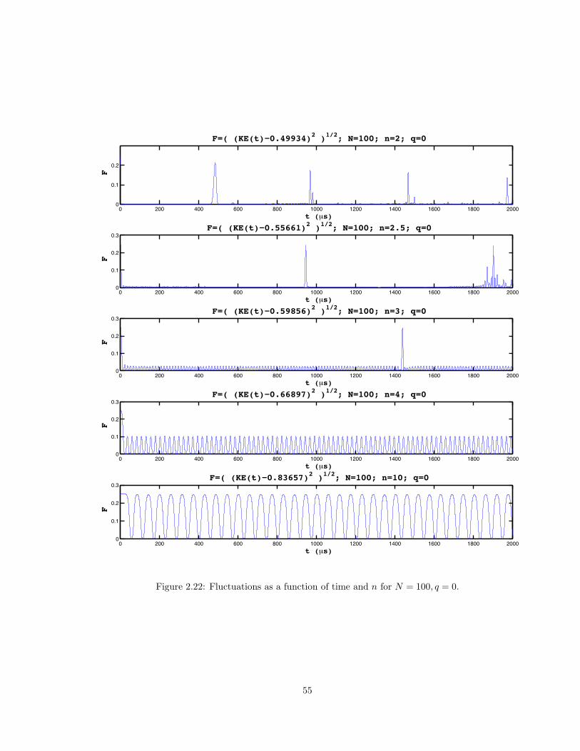
0 200 400 %00 &00 1000 1200 1400 1%00 1&00 20000

0"1

0"2

t (µs)

F

F=( (KE(t)−0.49934)2 )1/2; N=100; n=2; q=0

0 200 400 %00 &00 1000 1200 1400 1%00 1&00 20000

0"1

0"2

0"+

t (µs)

F

F=( (KE(t)−0.55661)2 )1/2; N=100; n=2.5; q=0

0 200 400 %00 &00 1000 1200 1400 1%00 1&00 20000

0"1

0"2

0"+

t (µs)

F

F=( (KE(t)−0.59856)2 )1/2; N=100; n=3; q=0

0 200 400 %00 &00 1000 1200 1400 1%00 1&00 20000

0"1

0"2

0"+

t (µs)

F

F=( (KE(t)−0.66897)2 )1/2; N=100; n=4; q=0

0 200 400 %00 &00 1000 1200 1400 1%00 1&00 20000

0"1

0"2

0"+

t (µs)

F

F=( (KE(t)−0.83657)2 )1/2; N=100; n=10; q=0

Figure 2.22: Fluctuations as a function of time and n for N = 100, q = 0.

55

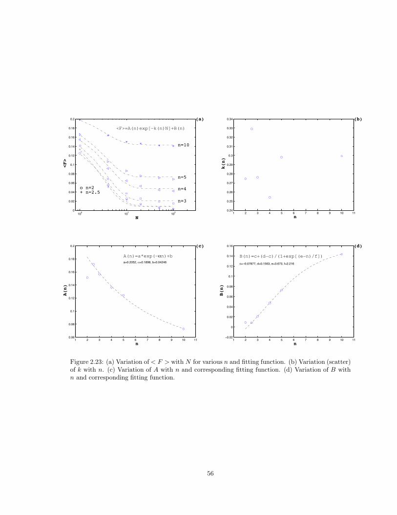
1 2 + 4 ( % - & , 10 110"0%

0"0&

0"1

0"12

0"14

0"1%

0"1&

0"2

n

A(n)

A(n)=a*exp(−!n)+ba*0"20(2? !*0"1&,&? J*0"0424%

(c)

1 2 + 4 ( % - & , 10 11!0"02

0

0"02

0"04

0"0%

0"0&

0"1

0"12

0"14

0"1%

n

B(n)

B(n)=c+(d−c)/(1+exp[(e−n)/f])

c*!0"0-&--? d*0"1(%+? e*+"%-+? K*2"21%

(d)

1 2 + 4 ( % - & , 10 110"24

0"2(

0"2%

0"2-

0"2&

0"2,

0"+

0"+1

0"+2

0"++

0"+4

n k(n)

(b)

100 101 1020

0"02

0"04

0"0%

0"0&

0"1

0"12

0"14

0"1%

0"1&

0"2

N

<F>

o n=2+ n=2.5

n=3

n=4

n=5

n=10

<F>=A(n)exp[−k(n)N]+B(n)

(a)

Figure 2.23: (a) Variation of < F > with N for various n and fitting function. (b) Variation (scatter)of k with n. (c) Variation of A with n and corresponding fitting function. (d) Variation of B withn and corresponding fitting function.

56

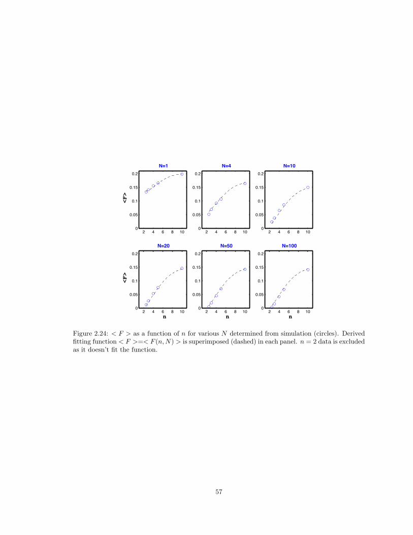
2 4 % & 100

0"0(

0"1

0"1(

0"2

<F>

N=1

2 4 % & 100

0"0(

0"1

0"1(

0"2

N=4

2 4 % & 100

0"0(

0"1

0"1(

0"2

N=10

2 4 % & 100

0"0(

0"1

0"1(

0"2

n

<F>

N=20

2 4 % & 100

0"0(

0"1

0"1(

0"2

n

N=50

2 4 % & 100

0"0(

0"1

0"1(

0"2

n

N=100

Figure 2.24: < F > as a function of n for various N determined from simulation (circles). Derivedfitting function < F >=< F (n, N) > is superimposed (dashed) in each panel. n = 2 data is excludedas it doesn’t fit the function.

57

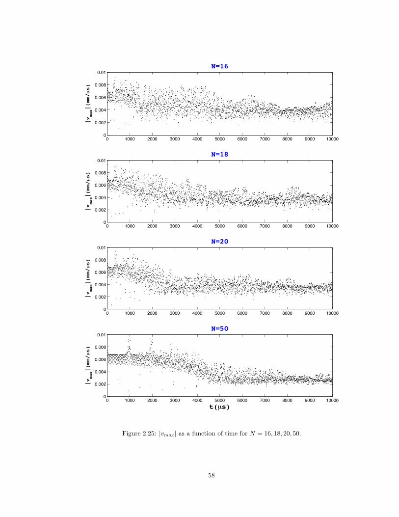
0 1000 2000 +000 4000 (000 %000 -000 &000 ,000 100000

0"002

0"004

0"00%

0"00&

0"01

|vmax|(mm/µs)

N=16

0 1000 2000 +000 4000 (000 %000 -000 &000 ,000 100000

0"002

0"004

0"00%

0"00&

0"01

|vmax|(mm/µs)

N=18

0 1000 2000 +000 4000 (000 %000 -000 &000 ,000 100000

0"002

0"004

0"00%

0"00&

0"01

|vmax|(mm/µs)

N=20

0 1000 2000 +000 4000 (000 %000 -000 &000 ,000 100000

0"002

0"004

0"00%

0"00&

0"01

|vmax|(mm/µs)

N=50

t(µs)

Figure 2.25: |vmax| as a function of time for N = 16, 18, 20, 50.

58

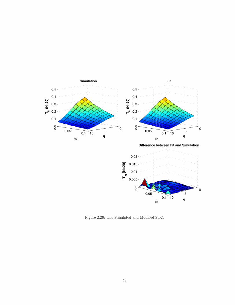
0(10

0 0"0(0"1

0

0"1

0"2

0"+

0"4

0"(

q

Simulation

&

TN

(N

=20)

0(10

00"0( 0"1

0

0"1

0"2

0"+

0"4

0"(

q

Fit

&

TN

(N

=20)

0(

10

00"0(

0"1

0

0"00(

0"01

0"01(

0"02

q

Difference between Fit and Simulation

&

TN (

N=2

0)

Figure 2.26: The Simulated and Modeled STC.

59

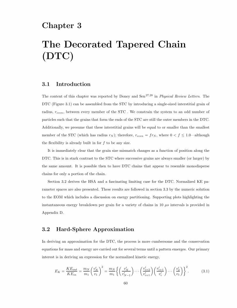
Chapter 3

The Decorated Tapered Chain(DTC)

3.1 Introduction

The content of this chapter was reported by Doney and Sen27,28 in Physical Review Letters. The

DTC (Figure 3.1) can be assembled from the STC by introducing a single-sized interstitial grain of

radius, reven, between every member of the STC . We constrain the system to an odd number of

particles such that the grains that form the ends of the STC are still the outer members in the DTC.

Additionally, we presume that these interstitial grains will be equal to or smaller than the smallest

member of the STC (which has radius rN ); therefore, reven = frN , where 0 < f ( 1.0—although

the flexibility is already built in for f to be any size.

It is immediately clear that the grain size mismatch changes as a function of position along the

DTC. This is in stark contrast to the STC where successive grains are always smaller (or larger) by

the same amount. It is possible then to have DTC chains that appear to resemble monodisperse

chains for only a portion of the chain.

Section 3.2 derives the HSA and a fascinating limiting case for the DTC. Normalized KE pa-

rameter spaces are also presented. These results are followed in section 3.3 by the numeric solution

to the EOM which includes a discussion on energy partitioning. Supporting plots highlighting the

instantaneous energy breakdown per grain for a variety of chains in 10 µs intervals is provided in

Appendix D.

3.2 Hard-Sphere Approximation

In deriving an approximation for the DTC, the process is more cumbersome and the conservation

equations for mass and energy are carried out for several terms until a pattern emerges. Our primary

interest is in deriving an expression for the normalized kinetic energy,

EK =KEout

KEin=

mN

m1

1v"Nv1

22

=mN

m1

51v"N

v"N!1

2· · ·

1v"i+2

v"i+1

21v"i+1

v"i

2· · ·

1v"2v1

262

. (3.1)

60

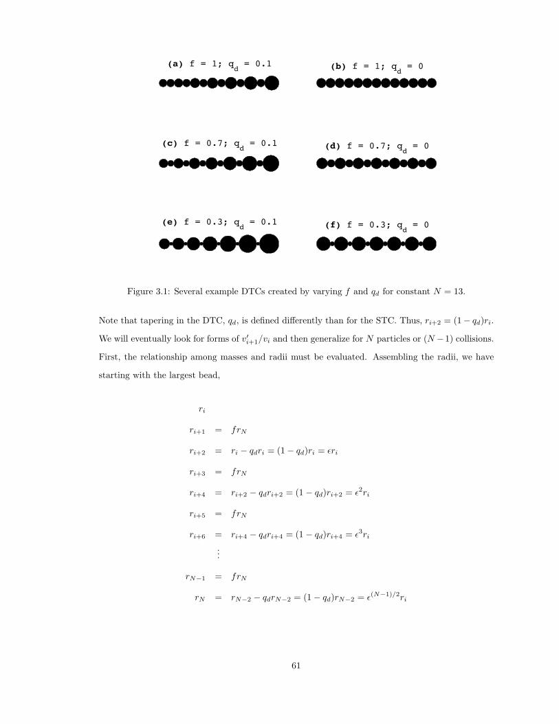
(a) f = 1; qd = 0.1 (b) f = 1; q

d = 0

(c) f = 0.7; qd = 0.1 (d) f = 0.7; q

d = 0

(e) f = 0.3; qd = 0.1 (f) f = 0.3; q

d = 0

Figure 3.1: Several example DTCs created by varying f and qd for constant N = 13.

Note that tapering in the DTC, qd, is defined di!erently than for the STC. Thus, ri+2 = (1$ qd)ri.

We will eventually look for forms of v"i+1/vi and then generalize for N particles or (N $1) collisions.

First, the relationship among masses and radii must be evaluated. Assembling the radii, we have

starting with the largest bead,

ri

ri+1 = frN

ri+2 = ri $ qdri = (1 $ qd)ri = $ri

ri+3 = frN

ri+4 = ri+2 $ qdri+2 = (1 $ qd)ri+2 = $2ri

ri+5 = frN

ri+6 = ri+4 $ qdri+4 = (1 $ qd)ri+4 = $3ri

...

rN!1 = frN

rN = rN!2 $ qdrN!2 = (1 $ qd)rN!2 = $(N!1)/2ri

61

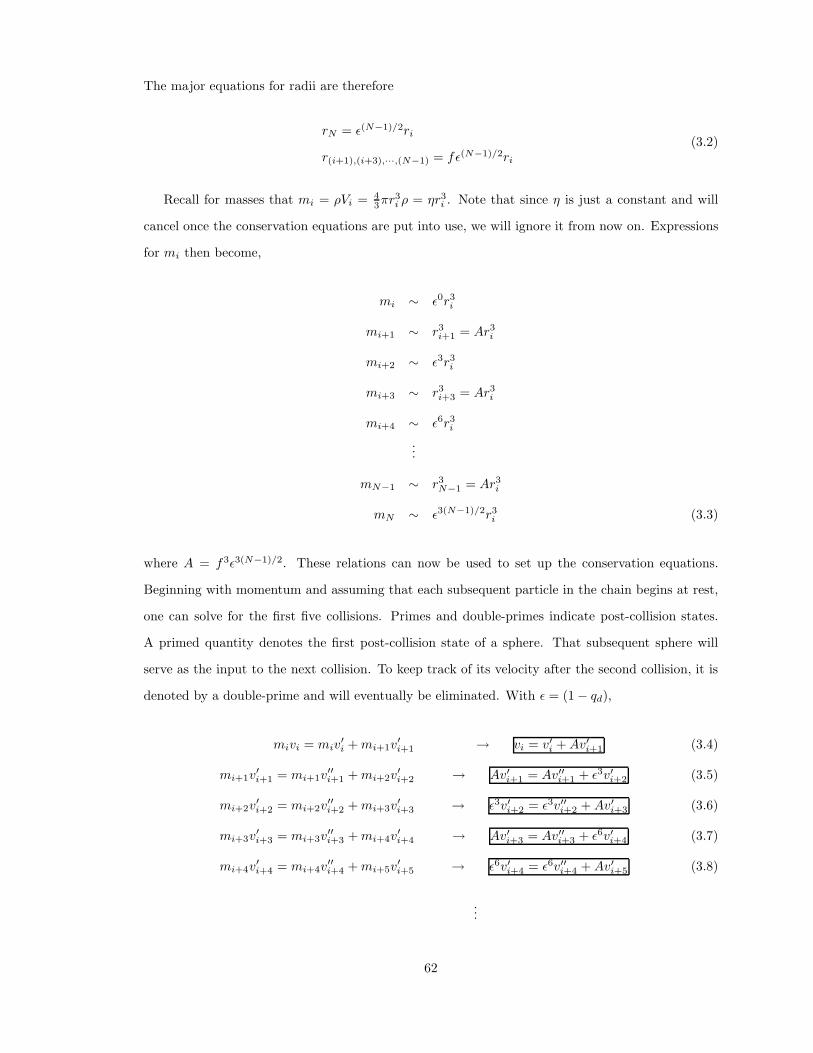
The major equations for radii are therefore

rN = $(N!1)/2ri

r(i+1),(i+3),···,(N!1) = f$(N!1)/2ri

(3.2)

Recall for masses that mi = (Vi = 43)r3

i ( = ,r3i . Note that since , is just a constant and will

cancel once the conservation equations are put into use, we will ignore it from now on. Expressions

for mi then become,

mi * $0r3i

mi+1 * r3i+1 = Ar3

i

mi+2 * $3r3i

mi+3 * r3i+3 = Ar3

i

mi+4 * $6r3i

...

mN!1 * r3N!1 = Ar3

i

mN * $3(N!1)/2r3i (3.3)

where A = f3$3(N!1)/2. These relations can now be used to set up the conservation equations.

Beginning with momentum and assuming that each subsequent particle in the chain begins at rest,

one can solve for the first five collisions. Primes and double-primes indicate post-collision states.

A primed quantity denotes the first post-collision state of a sphere. That subsequent sphere will

serve as the input to the next collision. To keep track of its velocity after the second collision, it is

denoted by a double-prime and will eventually be eliminated. With $ = (1 $ qd),

mivi = miv"i + mi+1v

"i+1 & vi = v"i + Av"i+1 (3.4)

mi+1v"i+1 = mi+1v

""i+1 + mi+2v

"i+2 & Av"i+1 = Av""i+1 + $3v"i+2 (3.5)

mi+2v"i+2 = mi+2v

""i+2 + mi+3v

"i+3 & $3v"i+2 = $3v""i+2 + Av"i+3 (3.6)

mi+3v"i+3 = mi+3v

""i+3 + mi+4v

"i+4 & Av"i+3 = Av""i+3 + $6v"i+4 (3.7)

mi+4v"i+4 = mi+4v

""i+4 + mi+5v

"i+5 & $6v"i+4 = $6v""i+4 + Av"i+5 (3.8)

...

62

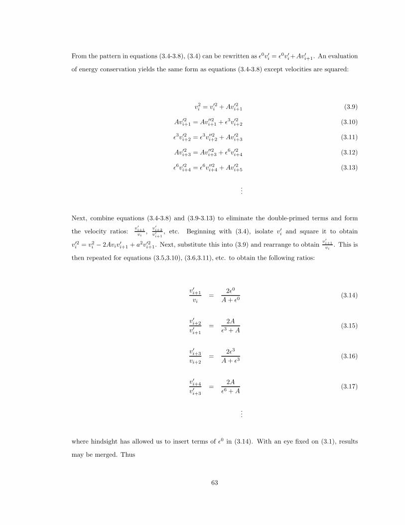
From the pattern in equations (3.4-3.8), (3.4) can be rewritten as $0v"i = $0v"i +Av"i+1. An evaluation

of energy conservation yields the same form as equations (3.4-3.8) except velocities are squared:

v2i = v"2i + Av"2i+1 (3.9)

Av"2i+1 = Av""2i+1 + $3v"2i+2 (3.10)

$3v"2i+2 = $3v""2i+2 + Av"2i+3 (3.11)

Av"2i+3 = Av""2i+3 + $6v"2i+4 (3.12)

$6v"2i+4 = $6v""2i+4 + Av"2i+5 (3.13)

...

Next, combine equations (3.4-3.8) and (3.9-3.13) to eliminate the double-primed terms and form

the velocity ratios: v!i+1vi

, v!i+2

v!i+1

, etc. Beginning with (3.4), isolate v"i and square it to obtain

v"2i = v2i $ 2Aviv"i+1 + a2v"2i+1. Next, substitute this into (3.9) and rearrange to obtain v!

i+1vi

. This is

then repeated for equations (3.5,3.10), (3.6,3.11), etc. to obtain the following ratios:

v"i+1

vi=

2$0

A + $0(3.14)

v"i+2

v"i+1

=2A

$3 + A(3.15)

v"i+3

vi+2=

2$3

A + $3(3.16)

v"i+4

v"i+3

=2A

$6 + A(3.17)

...

where hindsight has allowed us to insert terms of $0 in (3.14). With an eye fixed on (3.1), results

may be merged. Thus

63

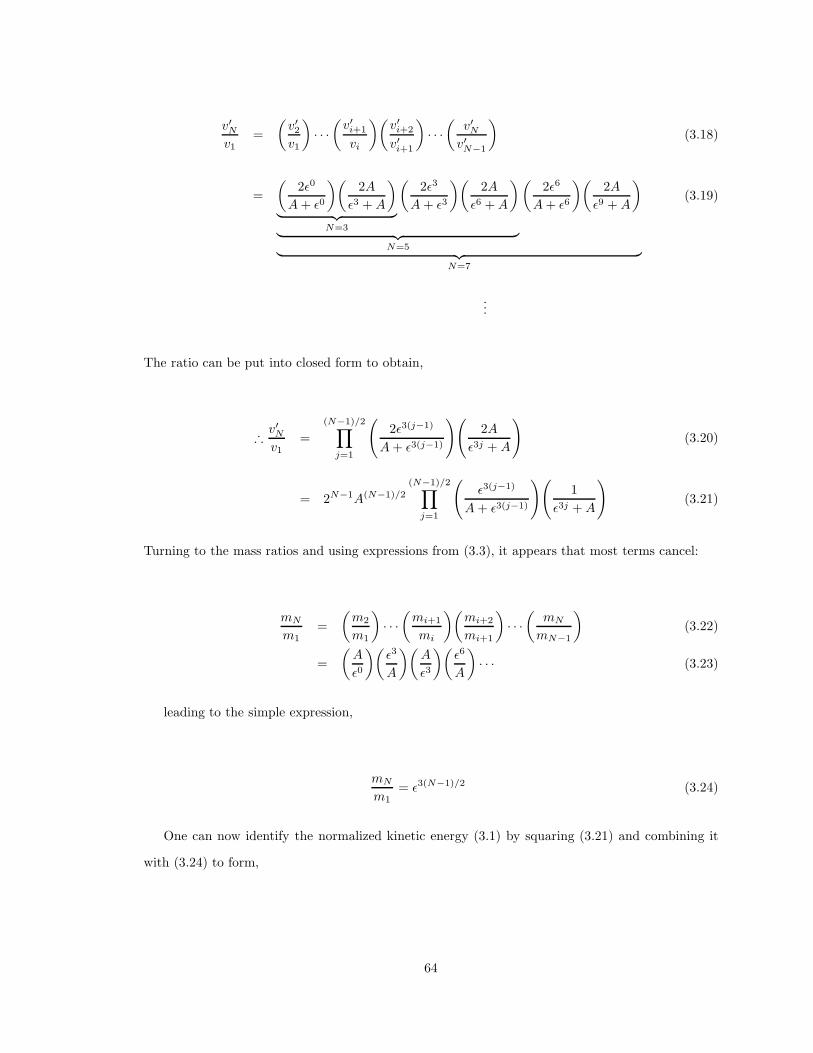
v"Nv1

=1

v"2v1

2· · ·

1v"i+1

vi

21v"i+2

v"i+1

2· · ·

1v"N

v"N!1

2(3.18)

=1

2$0

A + $0

212A

$3 + A

2

7 89 :N=3

12$3

A + $3

212A

$6 + A

2

7 89 :N=5

12$6

A + $6

212A

$9 + A

2

7 89 :N=7

(3.19)

...

The ratio can be put into closed form to obtain,

∴ v"Nv1

=(N!1)/2;

j=1

(2$3(j!1)

A + $3(j!1)

)(2A

$3j + A

)(3.20)

= 2N!1A(N!1)/2(N!1)/2;

j=1

($3(j!1)

A + $3(j!1)

)(1

$3j + A

)(3.21)

Turning to the mass ratios and using expressions from (3.3), it appears that most terms cancel:

mN

m1=

1m2

m1

2· · ·

1mi+1

mi

21mi+2

mi+1

2· · ·

1mN

mN!1

2(3.22)

=1

A

$0

21$3

A

21A

$3

21$6

A

2· · · (3.23)

leading to the simple expression,

mN

m1= $3(N!1)/2 (3.24)

One can now identify the normalized kinetic energy (3.1) by squaring (3.21) and combining it

with (3.24) to form,

64

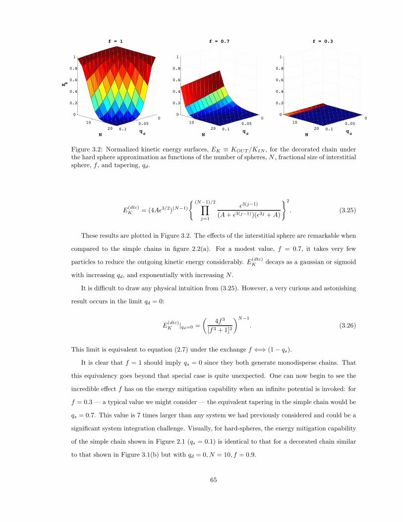
00.05

0.1

1020

0

0.2

0.4

0.6

0.8

1

q d

f = 1

N

E K

00.05

0.1

1020

0

0.2

0.4

0.6

0.8

1

q d

f = 0.7

N

00.05

0.1

1020

0

0.2

0.4

0.6

0.8

1

q d

f = 0.3

N

Figure 3.2: Normalized kinetic energy surfaces, EK ! KOUT /KIN , for the decorated chain underthe hard sphere approximation as functions of the number of spheres, N , fractional size of interstitialsphere, f , and tapering, qd.

E(dtc)K = (4A$3/2)(N!1)

"(N!1)/2;

j=1

$3(j!1)

(A + $3(j!1))($3j + A)

%2

. (3.25)

These results are plotted in Figure 3.2. The e!ects of the interstitial sphere are remarkable when

compared to the simple chains in figure 2.2(a). For a modest value, f = 0.7, it takes very few

particles to reduce the outgoing kinetic energy considerably. E(dtc)K decays as a gaussian or sigmoid

with increasing qd, and exponentially with increasing N .

It is di"cult to draw any physical intuition from (3.25). However, a very curious and astonishing

result occurs in the limit qd = 0:

E(dtc)K |qd=0 =

14f3

[f3 + 1]2

2N!1

. (3.26)

This limit is equivalent to equation (2.7) under the exchange f +, (1 $ qs).

It is clear that f = 1 should imply qs = 0 since they both generate monodisperse chains. That

this equivalency goes beyond that special case is quite unexpected. One can now begin to see the

incredible e!ect f has on the energy mitigation capability when an infinite potential is invoked: for

f = 0.3 — a typical value we might consider — the equivalent tapering in the simple chain would be

qs = 0.7. This value is 7 times larger than any system we had previously considered and could be a

significant system integration challenge. Visually, for hard-spheres, the energy mitigation capability

of the simple chain shown in Figure 2.1 (qs = 0.1) is identical to that for a decorated chain similar

to that shown in Figure 3.1(b) but with qd = 0, N = 10, f = 0.9.

65

3.3 Numeric Solution

3.3.1 KE Parameter Space Behavior

Figure 3.3 highlights the computational results for the decorated chain. Recall that the inertial

mismatch between neighboring grains in decorated chains change as a function of position along

the chain. This is what is believed to be the cause of a ripple in the surface of the EK plots that

propagate toward the origin as f decreases. As one might expect, such behavior is a function of

N, qd, and f . The e!ect vanishes for f ( 0.6, approximately. At about this threshold, the interstitial

grain is not much smaller (less massive) than the grains toward the end of the chain. The explanation

is that as an impulse propagates, energy transmission becomes increasingly e"cient due to smaller

inertial mismatches — a prerequisite for admitting solitary waves. Thus the system changes from a

shock absorber to shock transmitter. This e!ect however must compete with compressive e!ects in

some manner since no such behavior is present for hard spheres even though it too has a position-

dependent inertial mismatch.

The hard sphere approximation grossly exaggerates the shock mitigation capability of the deco-

rated chain. Additionally, it doesn’t pick up the surface feature resulting from a competition between

particle overlap nonlinearity and variable inertial mismatches between neighboring grains. Thus a

hard-sphere analysis is inadequate for the DTC. Simulations suggest that for f = 0.3, N = 5, qd = 0.1

(panel f), one can disperse energy within the chain such that only about 10% of that put into the

system is transmitted to the end with the initial pulse.

3.3.2 Energy Partition

A simple view of energy partitioning in the DTC is not possible given the vast number of possible

chain configurations, belittling those of the STC. Changing N has a much more severe impact on

the results because, by design, it a!ects the results everywhere in the chain. For example, if we take

the mass ratio of interstitial grains for N = 21 and N = 11 chains, with qd and f identical, the

results scale astonishingly: mN=21/mN=11 " (1 $ qd)15! For large tapering, qd = 0.1, interstitial

grains in a chain with N = 21 have about one-fifth the mass as their counterparts where N = 11.

Rather than focusing on the system, it is of interest to probe how a DTC partitions the energy

among particles as an impulse propagates. Figure 3.4 illustrates the instantaneous kinetic energy

per grain for various configurations at t = 52µs where qd = {0, 0.05, 0.1} and f = {1.0, 0.7, 0.3}.

Also included in each panel is a silhouette of the specific chain and the total kinetic energy of the

66

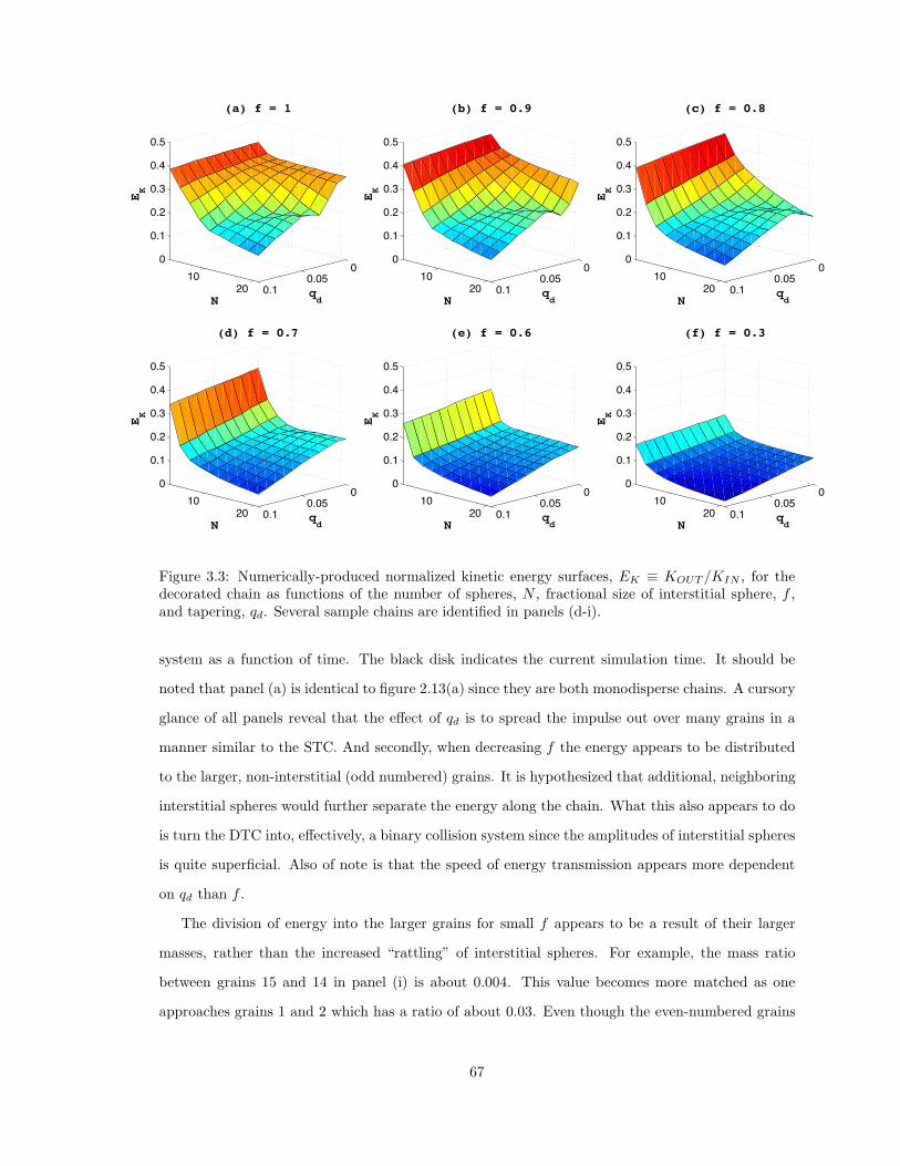
00"0(

0"110

20

0

0"1

0"2

0"+

0"4

0"(

qd

(a) f = 1

N

EK

00"0(

0"110

20

0

0"1

0"2

0"+

0"4

0"(

qd

(b) f = 0.9

N

EK

00"0(

0"110

20

0

0"1

0"2

0"+

0"4

0"(

qd

(c) f = 0.8

N

EK

00"0(

0"110

20

0

0"1

0"2

0"+

0"4

0"(

qd

(d) f = 0.7

N

EK

00"0(

0"110

20

0

0"1

0"2

0"+

0"4

0"(

qd

(e) f = 0.6

N

EK

00"0(

0"110

20

0

0"1

0"2

0"+

0"4

0"(

qd

(f) f = 0.3

N

EK

Figure 3.3: Numerically-produced normalized kinetic energy surfaces, EK ! KOUT /KIN , for thedecorated chain as functions of the number of spheres, N , fractional size of interstitial sphere, f ,and tapering, qd. Several sample chains are identified in panels (d-i).

system as a function of time. The black disk indicates the current simulation time. It should be

noted that panel (a) is identical to figure 2.13(a) since they are both monodisperse chains. A cursory

glance of all panels reveal that the e!ect of qd is to spread the impulse out over many grains in a

manner similar to the STC. And secondly, when decreasing f the energy appears to be distributed

to the larger, non-interstitial (odd numbered) grains. It is hypothesized that additional, neighboring

interstitial spheres would further separate the energy along the chain. What this also appears to do

is turn the DTC into, e!ectively, a binary collision system since the amplitudes of interstitial spheres

is quite superficial. Also of note is that the speed of energy transmission appears more dependent

on qd than f .

The division of energy into the larger grains for small f appears to be a result of their larger

masses, rather than the increased “rattling” of interstitial spheres. For example, the mass ratio

between grains 15 and 14 in panel (i) is about 0.004. This value becomes more matched as one

approaches grains 1 and 2 which has a ratio of about 0.03. Even though the even-numbered grains

67

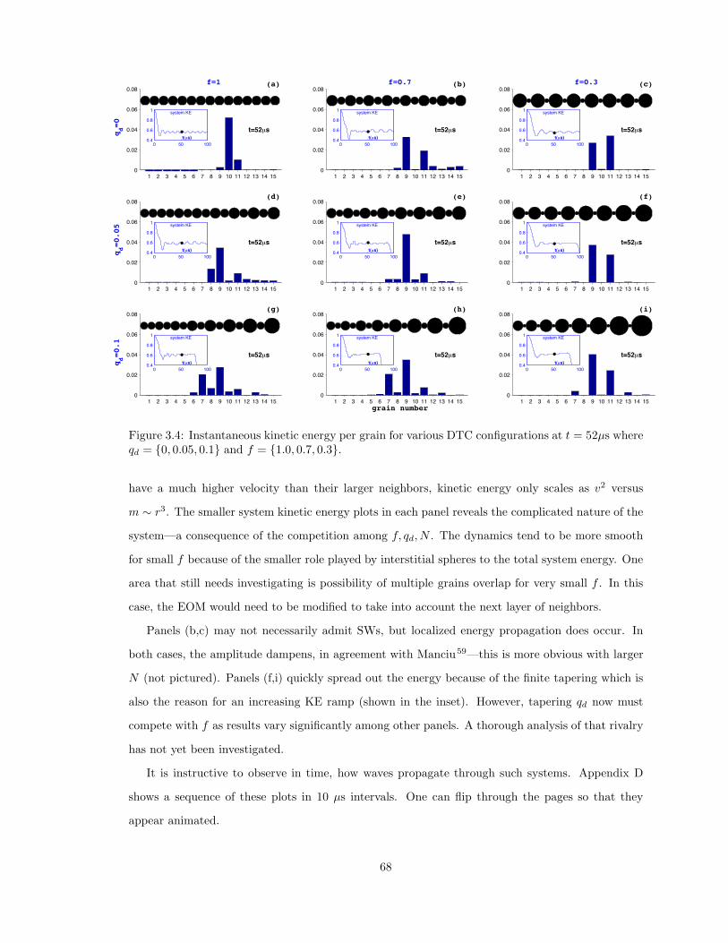
1 2 + 4 ( % - & , 10 11 12 1+ 14 1(0

0"02

0"04

0"0%

0"0&

t=52µs

qd=0

(a) f=1

0 (0 1000"4

0"%

0"&

1

t(µs)

system KE

1 2 + 4 ( % - & , 10 11 12 1+ 14 1(0

0"02

0"04

0"0%

0"0&

t=52µs

(b) f=0.7

0 (0 1000"4

0"%

0"&

1

t(µs)

system KE

1 2 + 4 ( % - & , 10 11 12 1+ 14 1(0

0"02

0"04

0"0%

0"0&

t=52µs

(c) f=0.3

0 (0 1000"4

0"%

0"&

1

t(µs)

system KE

1 2 + 4 ( % - & , 10 11 12 1+ 14 1(0

0"02

0"04

0"0%

0"0&

t=52µs

qd=0.05

(d)

0 (0 1000"4

0"%

0"&

1

t(µs)

system KE

1 2 + 4 ( % - & , 10 11 12 1+ 14 1(0

0"02

0"04

0"0%

0"0&

t=52µs

(e)

0 (0 1000"4

0"%

0"&

1

t(µs)

system KE

1 2 + 4 ( % - & , 10 11 12 1+ 14 1(0

0"02

0"04

0"0%

0"0&

t=52µs

(f)

0 (0 1000"4

0"%

0"&

1

t(µs)

system KE

1 2 + 4 ( % - & , 10 11 12 1+ 14 1(0

0"02

0"04

0"0%

0"0&

t=52µs

qd=0.1

(g)

0 (0 1000"4

0"%

0"&

1

t(µs)

system KE

1 2 + 4 ( % - & , 10 11 12 1+ 14 1(0

0"02

0"04

0"0%

0"0&

t=52µs

grain number

(h)

0 (0 1000"4

0"%

0"&

1

t(µs)

system KE

1 2 + 4 ( % - & , 10 11 12 1+ 14 1(0

0"02

0"04

0"0%

0"0&

t=52µs

(i)

0 (0 1000"4

0"%

0"&

1

t(µs)

system KE

Figure 3.4: Instantaneous kinetic energy per grain for various DTC configurations at t = 52µs whereqd = {0, 0.05, 0.1} and f = {1.0, 0.7, 0.3}.

have a much higher velocity than their larger neighbors, kinetic energy only scales as v2 versus

m * r3. The smaller system kinetic energy plots in each panel reveals the complicated nature of the

system—a consequence of the competition among f, qd, N . The dynamics tend to be more smooth

for small f because of the smaller role played by interstitial spheres to the total system energy. One

area that still needs investigating is possibility of multiple grains overlap for very small f . In this

case, the EOM would need to be modified to take into account the next layer of neighbors.

Panels (b,c) may not necessarily admit SWs, but localized energy propagation does occur. In

both cases, the amplitude dampens, in agreement with Manciu59—this is more obvious with larger

N (not pictured). Panels (f,i) quickly spread out the energy because of the finite tapering which is

also the reason for an increasing KE ramp (shown in the inset). However, tapering qd now must

compete with f as results vary significantly among other panels. A thorough analysis of that rivalry

has not yet been investigated.

It is instructive to observe in time, how waves propagate through such systems. Appendix D

shows a sequence of these plots in 10 µs intervals. One can flip through the pages so that they

appear animated.

68

Chapter 4

Hydrocode Simulations of TaperedChains

There are two reasons that stand out when considering the simulation of TCs in a hydrodynamics

code (hydrocode). The first is in probing the regime where plastic, and therefore permanent, de-

formation can occur. Secondly, it represents the next step towards the development of a potential

TC armor panel. This brief chapter describes preliminary e!orts in running such 2D and 3D simu-

lations. These results were presented at the March 2006 meeting of the American Physical Society

in Baltimore, MD.

ALEGRA18,79,110—or Arbitrary Lagrangian and Eulerian General Research Application—is a

massively parallel, finite element hydrodynamics code with modular physics capability developed

by Sandia National Laboratories. The general procedure for running such simulations consists of

mesh generation, simulation, and post-processing. The first step is performed using CUBIT22 which

discretizes the computational space. At each node, the conservation equations are solved using

ALEGRA. Finally, visualization is performed using Ensight17. While the manuals of the code are

publicly available, the software itself is export-controlled.

Both lagrangian and eulerian meshes have been considered for 3D and 2D meshes, respectively.

In the latter case, material advects through a stationary mesh1. This is in contrast to the Lagrangian

framework where the material is the mesh. An inherent di"culty in running Eulerian calculations,

is that mixed cells are endemic to the mesh. That is, any cell can be occupied by more than 1

material: part air, part water for example. As time progresses and the material advects through

the mesh, a code needs to keep track of that boundary between materials which has to be deter-

mined at a resolution finer than the mesh. This is known as interface tracking (IT) or interface

reconstruction (IR). Currently, ALEGRA supports16 three schemes: SLIC2, SMYRA3 8, and NEW

SMYRA. Results from simulations should be independent of the mesh (“mesh convergence”) as well

as the IT scheme, much in the way that physics is independent of a coordinate system. In Lagrange1More specifically, there is a lagrange step where the mesh deforms to follow the material and then is mapped back

into the eulerian mesh2Simple Line Interface Calculation3Sandia Modified Young’s Reconstruction Algorithm

69

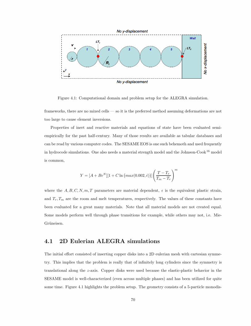
Figure 4.1: Computational domain and problem setup for the ALEGRA simulation.

frameworks, there are no mixed cells — so it is the preferred method assuming deformations are not

too large to cause element inversions.

Properties of inert and reactive materials and equations of state have been evaluated semi-

empirically for the past half-century. Many of those results are available as tabular databases and

can be read by various computer codes. The SESAME EOS is one such behemoth and used frequently

in hydrocode simulations. One also needs a material strength model and the Johnson-Cook16 model

is common,

Y = [A + B$N ][1 + C ln/max(0.002, $)

0]

(T $ Tr

Tm $ Tr

)m

where the A, B, C, N, m, T parameters are material dependent, $ is the equivalent plastic strain,

and Tr, Tm are the room and melt temperatures, respectively. The values of these constants have

been evaluated for a great many materials. Note that all material models are not created equal.

Some models perform well through phase transitions for example, while others may not, i.e. Mie-

Gruneisen.

4.1 2D Eulerian ALEGRA simulations

The initial e!ort consisted of inserting copper disks into a 2D eulerian mesh with cartesian symme-

try. This implies that the problem is really that of infinitely long cylinders since the symmetry is

translational along the z-axis. Copper disks were used because the elastic-plastic behavior in the

SESAME model is well-characterized (even across multiple phases) and has been utilized for quite

some time. Figure 4.1 highlights the problem setup. The geometry consists of a 5-particle monodis-

70

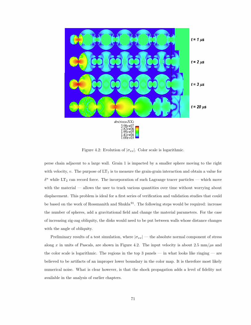
Figure 4.2: Evolution of |#xx|. Color scale is logarithmic.

perse chain adjacent to a large wall. Grain 1 is impacted by a smaller sphere moving to the right

with velocity, v. The purpose of LT1 is to measure the grain-grain interaction and obtain a value for

!n while LT2 can record force. The incorporation of such Lagrange tracer particles — which move

with the material — allows the user to track various quantities over time without worrying about

displacement. This problem is ideal for a first series of verification and validation studies that could

be based on the work of Rossmanith and Shukla91. The following steps would be required: increase

the number of spheres, add a gravitational field and change the material parameters. For the case

of increasing zig-zag obliquity, the disks would need to be put between walls whose distance changes

with the angle of obliquity.

Preliminary results of a test simulation, where |#xx| — the absolute normal component of stress

along x in units of Pascals, are shown in Figure 4.2. The input velocity is about 2.5 mm/µs and

the color scale is logarithmic. The regions in the top 3 panels — in what looks like ringing — are

believed to be artifacts of an improper lower boundary in the color map. It is therefore most likely

numerical noise. What is clear however, is that the shock propagation adds a level of fidelity not

available in the analysis of earlier chapters.

71

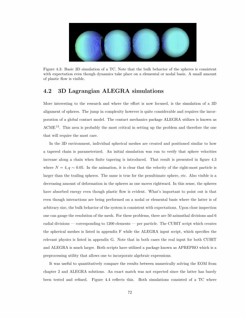
Figure 4.3: Basic 3D simulation of a TC. Note that the bulk behavior of the spheres is consistentwith expectation even though dynamics take place on a elemental or nodal basis. A small amountof plastic flow is visible.

4.2 3D Lagrangian ALEGRA simulations

More interesting to the research and where the e!ort is now focused, is the simulation of a 3D

alignment of spheres. The jump in complexity however is quite considerable and requires the incor-

poration of a global contact model. The contact mechanics package ALEGRA utilizes is known as

ACME13. This area is probably the most critical in setting up the problem and therefore the one

that will require the most care.

In the 3D environment, individual spherical meshes are created and positioned similar to how

a tapered chain is parameterized. An initial simulation was run to verify that sphere velocities

increase along a chain when finite tapering is introduced. That result is presented in figure 4.3

where N = 4, q * 0.05. In the animation, it is clear that the velocity of the right-most particle is

larger than the trailing spheres. The same is true for the penultimate sphere, etc. Also visible is a

decreasing amount of deformation in the spheres as one moves rightward. In this sense, the spheres

have absorbed energy even though plastic flow is evident. What’s important to point out is that

even though interactions are being performed on a nodal or elemental basis where the latter is of

arbitrary size, the bulk behavior of the system is consistent with expectations. Upon close inspection

one can gauge the resolution of the mesh. For these problems, there are 50 azimuthal divisions and 6

radial divisions — corresponding to 1200 elements — per particle. The CUBIT script which creates

the spherical meshes is listed in appendix F while the ALEGRA input script, which specifies the

relevant physics is listed in appendix G. Note that in both cases the real input for both CUBIT

and ALEGRA is much larger. Both scripts have utilized a package known as APREPRO which is a

preprocessing utility that allows one to incorporate algebraic expressions.

It was useful to quantitatively compare the results between numerically solving the EOM from

chapter 2 and ALEGRA solutions. An exact match was not expected since the latter has barely

been tested and refined. Figure 4.4 reflects this. Both simulations consisted of a TC where

72

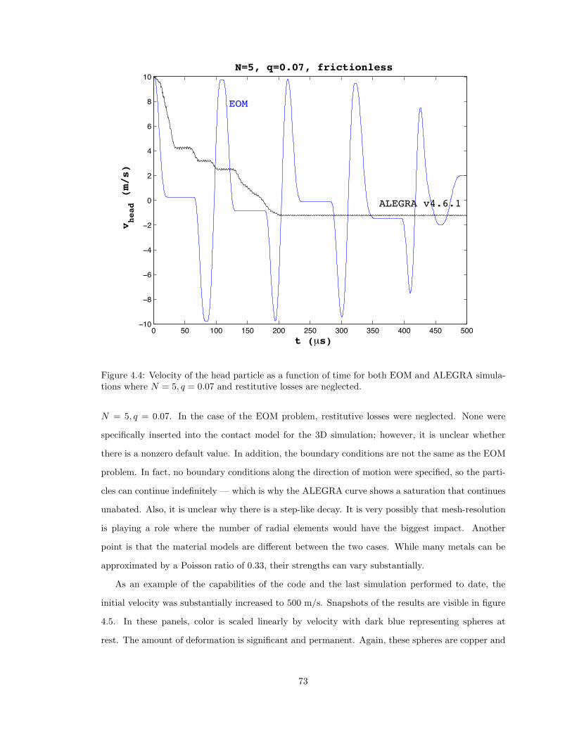
0 (0 100 1(0 200 2(0 +00 +(0 400 4(0 (00!10

!&

!%

!4

!2

0

2

4

%

&

10

t (µs)

vhead (m/s)

ALEGRA v4.6.1

EOM

N=5, q=0.07, frictionless

Figure 4.4: Velocity of the head particle as a function of time for both EOM and ALEGRA simula-tions where N = 5, q = 0.07 and restitutive losses are neglected.

N = 5, q = 0.07. In the case of the EOM problem, restitutive losses were neglected. None were

specifically inserted into the contact model for the 3D simulation; however, it is unclear whether

there is a nonzero default value. In addition, the boundary conditions are not the same as the EOM

problem. In fact, no boundary conditions along the direction of motion were specified, so the parti-

cles can continue indefinitely — which is why the ALEGRA curve shows a saturation that continues

unabated. Also, it is unclear why there is a step-like decay. It is very possibly that mesh-resolution

is playing a role where the number of radial elements would have the biggest impact. Another

point is that the material models are di!erent between the two cases. While many metals can be

approximated by a Poisson ratio of 0.33, their strengths can vary substantially.

As an example of the capabilities of the code and the last simulation performed to date, the

initial velocity was substantially increased to 500 m/s. Snapshots of the results are visible in figure

4.5. In these panels, color is scaled linearly by velocity with dark blue representing spheres at

rest. The amount of deformation is significant and permanent. Again, these spheres are copper and

73

simulations have not yet been performed with other metals. In the last panel, the copper “pancakes”

are still moving at approximately 250 m/s.

As a final note, many interesting questions can now be asked and explored with the use of

ALEGRA. While testing of the systems and proper and careful setup still need to be performed, there

is now the capability to investigate the combined e!ects of many TCs. Antiparallel arrangements

can be inserted into the mesh and surrounded by other metals, insulators, etc. These can be encased

by various alloys of steel and struck with a flyer plate (see figure 5.1. The resulting force can be

measured on the output by surface tools in the visualization software. In addition, (virtual) tracer

particles can be put at arbitrary locations to monitor local e!ects. The possibilities are actually

quite staggering — stay tuned.

74

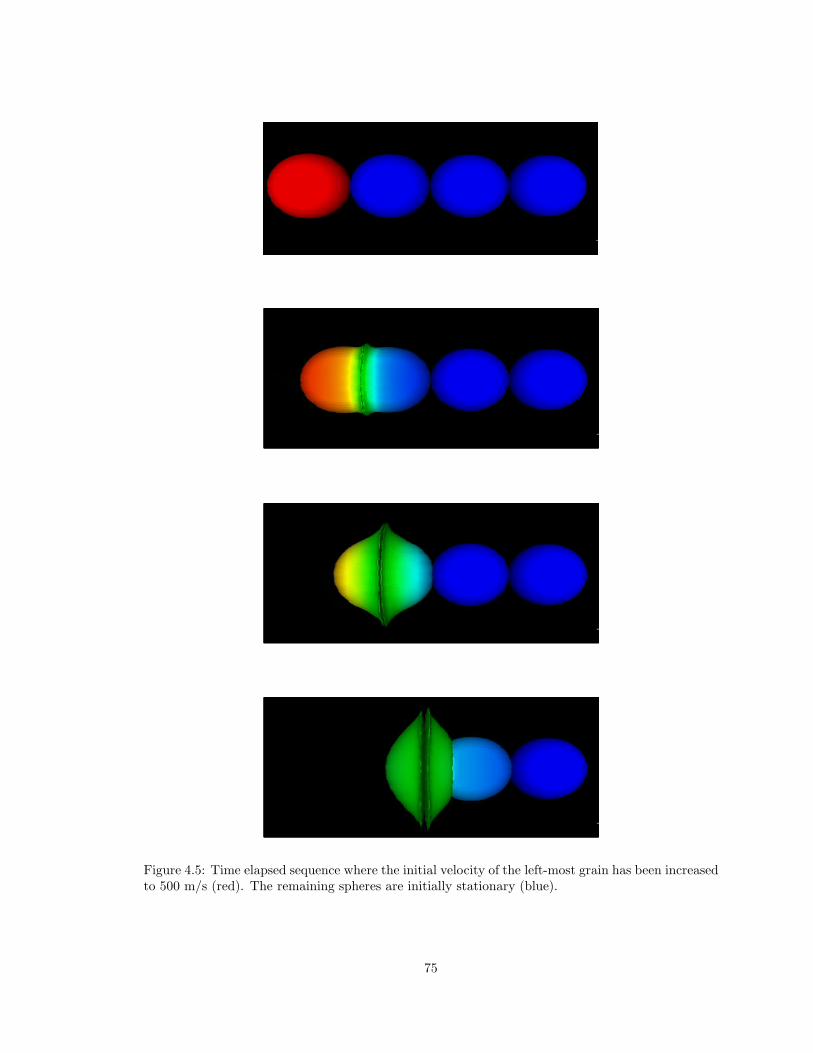
Figure 4.5: Time elapsed sequence where the initial velocity of the left-most grain has been increasedto 500 m/s (red). The remaining spheres are initially stationary (blue).

75

Chapter 5

Closing Remarks

On March 12, 2006, Joe Ray — a close family friend, employee of Buncombe County in Asheville,

NC, and an explosives ordnance specialist — was clearing mines for civilian and coalition tra"c

in Asadabad, Afghanistan during Operation Enduring Freedom. The up-armored humvee that

was carrying him, Sgt. Kevin Akins, Spc. Joshua Hill, and Sgt. Anton Hiett of the 391st Engineer

Battalion4,12 was hit by a stationary and camoflauged improvised explosive device. No one survived.

Such vehicles are overmatched by the seemingly endless quantity of explosive that can be put into

such contemptible devices. It is just one example — and a personal one — where there will always

be a need to improve our ability in absorbing blast energy. While the technology that has been

discussed in this dissertation is not claiming to be able to mitigate the meganewtons of force that

such blasts can generate, it represents the basic research which hopefully paves the way for us to get

there. To that end, we have investigated the shock mitigation and nonlinear dynamical properties

— as it pertains to the partition of energy — of tapered metal spheres arranged in one-dimensional

arrays.

The analysis has been carried out where two chain geometries are of particular interest: the

simple tapered chain (STC: figure 2.1) and the decorated tapered chain (DTC: figure 3.1). These

systems exhibit strongly nonlinear behavior due to the Hertz potential which has been used to govern

the contact mechanics in solving the equations of motion for each sphere. The dynamics and shock

mitigation properties of each chain have been analyzed as functions of the relevant parameters.

These are constant for each chain and are defined as the number of spheres, the tapering, and the

coe"cient of restitution. For the DTC, there is an additional parameter, f , which governs the size of

interstitial spheres used to increase the inertial mismatch between neighboring grains. The following

conclusions with a short summary is o!ered.

76

Both chain geometries decimate impulses substantially.

It is clear from the experiments performed by others and the simulations and data presented here

that both the STC and DTC decimate impulses. Further, the DTC can outperform the STC in fewer

spheres, making it desirable in applications where little space is available. The primary mechanism

responsible is symmetry breaking, or inertial mismatches between neighboring grains. Essentially,

momentum and energy remain trapped in the donor sphere thus spreading an impulse out in time and

space as it propagates through a chain. This is repeated at each interface where there is a mismatch.

For equally-sized spheres, solitary waves (SW) propagate and symmetry is maintained except at the

boundary. Once the boundary is reached, the SW is reconstructed, but imperfectly. That left-over

energy goes into the creation of secondary solitary waves (SSW) which have the same width, but

travel at smaller velocities due to the small amplitudes. This process continues indefinitely. In the

DTC, the e!ect of qd is to spread the impulse out over many grains in a manner similar to the STC.

Secondly, the role of decreasing f is it distribute energy to the larger, non-interstitial grains. By

increasing the number of interstitial grains, it is hypothesized that energy would continue to spread

out and remain trapped in the larger grains. This has applications for redirecting the energy if those

sites were su"ciently coupled to some transit channel — making the problem 2D or 3D. One could

also potentially increase dissipation with clever selection of materials.

A hard-sphere approximation is valid for the STC but invalid for the DTC.

Normalized energy and force surfaces were evaluated to measure each chain’s trapping ability. In

considering the STC, results indicate that there is a sigmoidal or gaussian decay on q and an

exponential dependence on N . This trend is consistent with the results from numerically solving

the equations of motion. For the DTC however, the hard-sphere analysis and numerical solution are

markedly di!erent in terms of the former missing phenomenology and greatly over-predicting energy

absorption.

The DTC hard-sphere approximation reduces to the STC in a special limit.

It was quite surprising that in the limit qd = 0, equation (3.25) — which describes the shock

absorption quality of a DTC for N, q, f — reduces to equation (2.7) under the exchange f +,

(1 $ qs). This says that a hard-sphere chain, consisting of an alternating series of radii (where

rsmall = frlarge), has the kinetic energy absorption equivalency of a STC with tapering qs.

77

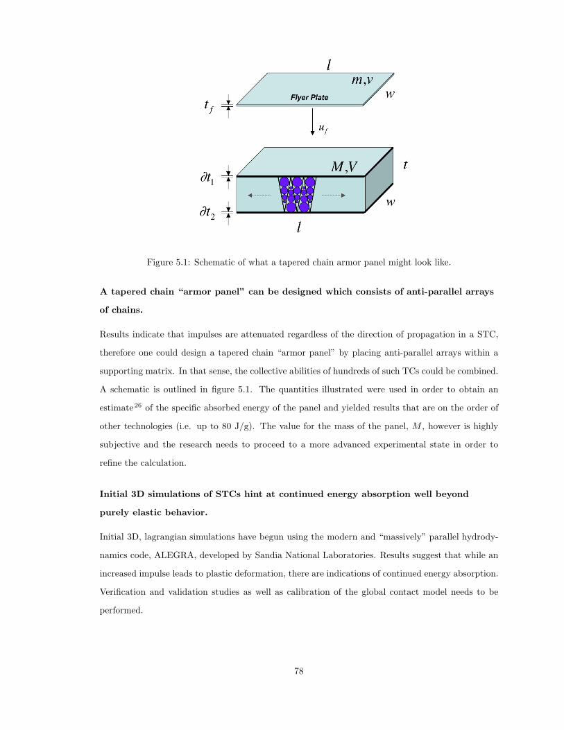
Figure 5.1: Schematic of what a tapered chain armor panel might look like.

A tapered chain “armor panel” can be designed which consists of anti-parallel arrays

of chains.

Results indicate that impulses are attenuated regardless of the direction of propagation in a STC,

therefore one could design a tapered chain “armor panel” by placing anti-parallel arrays within a

supporting matrix. In that sense, the collective abilities of hundreds of such TCs could be combined.

A schematic is outlined in figure 5.1. The quantities illustrated were used in order to obtain an

estimate26 of the specific absorbed energy of the panel and yielded results that are on the order of

other technologies (i.e. up to 80 J/g). The value for the mass of the panel, M , however is highly

subjective and the research needs to proceed to a more advanced experimental state in order to

refine the calculation.

Initial 3D simulations of STCs hint at continued energy absorption well beyond

purely elastic behavior.

Initial 3D, lagrangian simulations have begun using the modern and “massively” parallel hydrody-

namics code, ALEGRA, developed by Sandia National Laboratories. Results suggest that while an

increased impulse leads to plastic deformation, there are indications of continued energy absorption.

Verification and validation studies as well as calibration of the global contact model needs to be

performed.

78

An expression for the period of a single particle in the overlap potential has been

evaluated.

Equation (1.11) quantifies the period of a single particle in the overlap potential, of arbitrary power

n and input velocity, vi.

STCs do not equipartition energy but they do satisfy the virial theorem.

Equipartition can be spoken of either at a system level or for individual particles. In the former,

equipartition is not satisfied, but discrete systems with arbitrary n in the overlap potential were

found to obey the virial theorem. At a particle level, certain chains showed a tendency to equally

partition the available KE to all members after su"cient time had transpired.

Even after long simulation time, STCs still fluctuate about the system’s mean kinetic

energy. They appear to settle into a quasi-equilibrium.

While the mean value of KE in STCs was found to obey the virial theorem and particle veloci-

ties demonstrate a Gaussian profile, the system settles into a volatile state referred to as quasi-

equilibrium. The fluctuations remain quite measurable even over long simulation time and their

mean value has been quantified as a function of the number of particles and the exponent in the

overlap potential (equation 2.13).

A great number of questions still need to be investigated.

In concluding this dissertation, I pose the following research areas for further study beyond the

endless topics and questions that the 3D simulations pose.

• A close inspection of figure 2.23(a) for n = 2, 2.5 indicates that equation (2.13) governing the

decay in the mean fluctuations may not be su"ciently robust. It would be useful to run the

simulations where N = 500 or N = 103 to improve the formulation. Also, why does < F >

appear to be independent of q?

• Daraio23 has experimentally verified shock absorption in chains where the material properties

have been varied. What can be learned from numerical simulations, say for material and size

variation?

• Is it possible to exploit the phenomenon of inelastic collapse for shock mitigation purposes?

79

• What is the proper way to characterize quasi-equilibrium? Should it be based on equilibrium

conditions of a particular state of matter or combinations thereof?

• What does the stress-strain curve of a TC look like?

• What is the best filler material in a tapered chain armor panel?

80

Appendix A

STC Code from Pfannes80

/* PROGRAM taperchain.cpp

ORIGINAL VERSION: J.M.M. Pfannes

This program consideres an one dimensional chain of spheres that

shrink succesively in radius ("tapered chain"). Initially the spheres

are barely in contact, i. e. they just touch each other and are not

compressed (zero loading).

The chain ends at both edges at fixed walls.

The program calculates the interaction of the system once disturbed

by an instantaneous (delta) impulse exerted on one end of the chain.

Restitution both between the spheres and between the edge spheres

and the corresponding wall can be introduced.

The program does not consider gravity.

The EOM are solved with the Velocity Verlet algorithm.

scale of problem: mm-mg-musec (mimimu)

in this scale unit of force: 1000 N

in this scale unit of energy: 1 J

*/

#include <cmath>

#include <iostream>

#include <fstream>

81

#include <cstdlib>

#include <string>

#include <sstream>

using namespace std;

/************************** ALTERABLE PARAMETER: ****************************/

const int nptles=20; // total number of particles

const double rho=3.2 /* SiC (mg/mm^3) */, D=0.00326603139013 /* (mm^2/N) */;

const double rlarge = 5.0; // (radius of large ptle (mm))

const double q = 0.0; // (tapering factor (%))

const double xn = 2.5; // (exponent in potential)

const double dt = 0.00001; // (timestepwidth (musec))

const unsigned int nsteps = 100000000; // (# steps integration loop)

const int idiagp = 20000; // (stepwidth diagnostics)

const int idump = 20000; // (stepwidth dump)

const double v1in = 0.0; // (initial v small ptle (mm/musec))

const double vnin = -0.01; // initial v large ptle (mm/musec))

const double epsilon = 1.0; // ((1 - restitution factor) all ptles)

/****************************************************************************/

ofstream readme("taperchain.readme"); // global scope fcts

ofstream EnergyImpulse("taperchain.EneImp");

void radii (double rlocal[]) {

rlocal[nptles-1] = rlarge;

if (q == 0) // avoid roundoff errors w/out tapering

for (int i = 0; i < nptles-1; i++)

rlocal[i] = rlarge;

else

for (int i = 2; i < nptles+1; i++)

rlocal[nptles-i] = rlocal[nptles-i+1] * (1 - q*0.01);

82

}

void masses (double r[], double masslocal[]) {

const double pi = 4 * atan(1.0);

const double masslarge = (4.0/3.0) * pi * rlarge*rlarge*rlarge * rho;

masslocal[nptles-1] = masslarge;



masslocal[i] = masslarge;

else


masslocal[i] = r[i]*r[i]*r[i] * masslarge / (rlarge*rlarge*rlarge);

}

void strenghtfac (double r[], double alocal[]) {

alocal[0] = (2.0 / (5.0 * D)) * (sqrt(r[0]));

alocal[nptles] = (2.0 / (5.0 * D)) * (sqrt(r[nptles-1]));


for (int i = 1; i < nptles; i++)

alocal[i] = (2.0 / (5.0*D)) * (sqrt(0.5*rlarge));

else


alocal[i] = (2.0 / (5.0 * D)) * (sqrt((r[i]*r[i-1])/(r[i]+r[i-1])));

}

// initialpos prints absolute initial positions, not for calculations

void initialpos (double r[], double xInitiallocal[]) {



xInitiallocal[i] = (2.0*(i+1) - 1) * rlarge;

else {

xInitiallocal[0] = r[0];


83

xInitiallocal[i] = xInitiallocal[i-1] + r[i-1] + r[i];

}

}

// absolutpos prints absolute positions to ptle files, not for calculations

void absolutpos (double r[], double x[],

double xInitial[], double xAbsolutlocal[]) {


xAbsolutlocal[i] = xInitial[i] + x[i];

}

void computeAccelerations (double x[], double a[], double r[],

double acc[], double overbefore[],

double mass[], double& pot) {

pot = 0.0; // every call calculates new pot contributions

for (int i = 0; i < nptles; i++) // zeroing all acc in every call

acc[i] = 0.0; // (= every timestep)

/******* potential/force between neighboring ptles *****************/

for (int i = 0; i < nptles-1; i++) {

if (x[i] > x[i+1]) { // only when overlap

double over = x[i] - x[i+1];

double overnm1 = pow(over, (xn - 1.0));

pot += over * overnm1 * a[i+1];

double forceBetw = a[i+1] * xn * overnm1;

double forceFactor;

if (overbefore[i+1] < over) // when compressing

forceFactor = 1.0;

else forceFactor = epsilon; // when decompressing

84

forceBetw *= forceFactor;

// dim acc: force

acc[i] -= forceBetw; // sign(-): towards smaller x

acc[i+1] += forceBetw; // sign(+): towards larger x

overbefore[i+1] = over; // update for next timestep

}

else overbefore[i+1] = 0.0; // reset when no overlap

}

/** potential/force between fixed wall (small, x=0) <-> small ptle **/

if (x[0] < 0) {

double over = - x[0];


pot += over * overnm1 * a[0];

double forceSmall = a[0] * xn * overnm1;

double forceFactor;

if (overbefore[0] < over)

forceFactor = 1.0;

else forceFactor = epsilon;

forceSmall *= forceFactor;

acc[0] += forceSmall;

overbefore[0] = over;

}

else overbefore[0] = 0.0;

/*** potential/force between fixed wall (large) <-> large ptle ******/

if (x[nptles-1] > 0) {

double over = x[nptles-1];

85


pot += over * overnm1 * a[nptles];

double forceLarge = a[nptles] * xn * overnm1;

double forceFactor;

if (overbefore[nptles] < over)

forceFactor = 1.0;

else forceFactor = epsilon;

forceLarge *= forceFactor;

acc[nptles-1] -= forceLarge;

overbefore[nptles] = over;

}

else overbefore[nptles] = 0.0;

/***** real dim of acc: division by mass **********/


acc[i] /= mass[i];

}

void velocityVerletStep (double x[], double v[], double acc[],

double a[], double r[], double overbefore[],

double mass[], double& pot) {

for (int j = 0; j < nptles; j++) {

x[j] += v[j] * dt + 0.5 * acc[j] * dt*dt;

v[j] += 0.5 * acc[j] * dt;

}

computeAccelerations (x, a, r, acc, overbefore, mass, pot);

86

for (int j = 0; j < nptles; j++)

v[j] += 0.5 * acc[j] * dt;

}

void ptleHeader (ofstream* print, int k) {

(* print) << "# ptle " << k+1 << ": time (musec)" << ’\t’ << "x (mm)"

<< ’\t’ << "v (mm/musec)" << ’\t’ << "a (mm/musec^2)"

<< ’\t’ << "kin. E. (J)" << ’\t’ << "f (kN)" << ’\t’

<< "impulse (mg*mm/musec)" << ’\t’ << "xRelative (mm)" << ’\n’;

}

void dumpData (double t, double mass[], double v[], double acc[],

double r[], double x[], // scope absolutpos

double xInitial[], double xAbsolut[],

ofstream* print, int k) {

double keDumpPt[nptles]; // new arrays for dumping data

double vDumpPt[nptles]; // since arrays pass by argument

double accDumpPt[nptles]; // dump data manipulated

double xDumpPt[nptles];

keDumpPt[k] = 0.5 * mass[k] * v[k]*v[k];

if (keDumpPt[k] < 1.0e-20) keDumpPt[k] = 0.0; // set small values to zero

vDumpPt[k] = v[k];

if (vDumpPt[k] < 1.0e-20 && vDumpPt[k] > -1.0e-20) vDumpPt[k] = 0.0;

accDumpPt[k] = acc[k];

if (accDumpPt[k] < 1.0e-20 && accDumpPt[k] > -1.0e-20) accDumpPt[k] = 0.0;

xDumpPt[k] = x[k];

if (xDumpPt[k] < 1.0e-20 && xDumpPt[k] > -1.0e-20) xDumpPt[k] = 0.0;

87

absolutpos (r, x, xInitial, xAbsolut); // calculate absolute pos.

(* print) << t << ’\t’ << xAbsolut[k] << ’\t’ << vDumpPt[k] << ’\t’

<< accDumpPt[k] << ’\t’ << keDumpPt[k] << ’\t’

<< accDumpPt[k]*mass[k] << ’\t’

<< mass[k]*vDumpPt[k] << ’\t’ << xDumpPt[k] << ’\n’;

}

void dumpEnergyImpulse (double t, double kelocal, double telocal, double pot,

double ptotallocal, double mass[], double v[]) {

kelocal = 0.0;

ptotallocal = 0.0;

double absptotallocal = 0.0; // scope only within function

for (int j = 0; j < nptles; j++) {

kelocal += mass[j] * v[j]*v[j];

ptotallocal += mass[j] * v[j];

absptotallocal += mass[j] * abs(v[j]);

}

kelocal *= 0.5;

telocal = kelocal + pot;

double potDump = pot;

if (kelocal < 1.0e-20) kelocal = 0.0; // set very small values to zero

if (ptotallocal < 1.0e-20 && ptotallocal > -1.0e-20) ptotallocal = 0.0;

if (telocal < 1.0e-20) telocal = 0.0;

if (potDump < 1.0e-20) potDump = 0.0;

if (absptotallocal < 1.0e-20) absptotallocal = 0.0;

EnergyImpulse.precision(16);

EnergyImpulse << t << ’\t’ << kelocal << ’\t’ << potDump << ’\t’

<< telocal << ’\t’ << absptotallocal << ’\t’

<< ptotallocal << ’\n’;

}

88

void readmeInfo (double ke, double pot, double te, double ptotal,

double ke1in, double kenin, double p1in, double pnin,

double r[], double xInitial[], double mass[],

double a[]) {

readme << ’\t’ << ":-) *** TAPERCHAIN within walls *** (-:"

<< ’\n’ << ’\n’;

readme << "parameter of this run: " << ’\n’ << ’\n’;

readme << "total number of particles: " << ’\t’ << ’\t’ << nptles << ’\n’;

readme << "density of particles (mg/mm^3): " << ’\t’ << rho << ’\n’;

readme << "quantity D of particles (mm^2/N): " << ’\t’ << D << ’\n’;

readme << "radius of large ptle (mm): " << ’\t’ << ’\t’ << rlarge << ’\n’;

readme << "tapering factor (%): " << ’\t’ << ’\t’ << ’\t’ << q << ’\n’;

readme << "exponent in potential: " << ’\t’ << ’\t’ << ’\t’ << xn << ’\n’;

readme << "timestepwidth (musec): " << ’\t’ << ’\t’ << ’\t’ << dt << ’\n’;

readme << "# steps integration loop: " << ’\t’ << ’\t’ << nsteps << ’\n’;

readme << "stepwidth diagnostics: " << ’\t’ << ’\t’ << ’\t’ << "every "

<< idiagp << " timesteps" << ’\n’;

readme << "stepwidth dump: " << ’\t’ << ’\t’ << ’\t’ << "every "

<< idump << " timesteps" << ’\n’;

readme << "initial v small ptle (mm/musec): " << ’\t’ << v1in << ’\n’;

readme << "initial v large ptle (mm/musec): " << ’\t’ << vnin << ’\n’;

readme << "restitution factor for all ptles: " << ’\t’ << 1-epsilon << ’\n’

<< ’\n’;

readme << "total length of run (musec): " << ’\t’ << dt * nsteps << ’\n’;

readme << "total rows recorded for .EneImp file: " << ’\t’ << ’\t’

<< nsteps/idiagp +1 << ’\n’;

readme << "total rows recorded for particle files: " << ’\t’

<< nsteps/idump +1 << ’\n’ << ’\n’;

readme << "Initial system info (t=0): " << ’\n’ << ’\n’;

readme << "kin. E. (J)" << ’\t’ << "pot. E. (J)" << ’\t’

<< "tot. E. (J)" << ’\t’ << "total impulse (mg*mm/musec)" << ’\n’;

89

readme << ke << ’\t’ << pot << ’\t’ << te << ’\t’ << ptotal

<< ’\n’ << ’\n’;

readme << "kin. E. of small particle (J): " << ’\t’ << ’\t’ << ke1in

<< ’\n’;

readme << "kin. E. of large particle (J): " << ’\t’ << ’\t’ << kenin

<< ’\n’;

readme << "impulse of small particle (mg*mm/musec): " << ’\t’

<< p1in << ’\n’;

readme << "impulse of large particle (mg*mm/musec): " << ’\t’

<< pnin << ’\n’ << ’\n’;

readme << "particle radii (mm): " << ’\n’;

for (int i=0; i < nptles; i++) {

readme << r[i] << ’\t’;

}

readme << ’\n’ << ’\n’;

readme << "initial particle positions (mm): " << ’\n’;


readme << xInitial[i] << ’\t’;

}

readme << ’\n’ << ’\n’;

readme << "total length of one dimensional alignment (mm): " << ’\t’

<< xInitial[nptles-1] + r[nptles-1] << ’\n’ << ’\n’;

readme << "particle masses (mg): " << ’\n’;


readme << mass[i] << ’\t’;

}

readme << ’\n’ << ’\n’;

readme << "particle interaction strenghts (0.0316*N/mm^(3/2)): " << ’\n’;

for (int i=0; i < nptles+1; i++) {

readme << a[i] << ’\t’;

}

readme << ’\n’;

}

90

int main ( ) {

double r[nptles], x[nptles], xAbsolut[nptles], xInitial[nptles],

v[nptles], acc[nptles], mass[nptles], a[nptles+1],

overbefore[nptles+1], pot;

/******************** functions *****************************/

radii (r);

masses (r, mass);

strenghtfac (r, a);

initialpos (r, xInitial);

/********************** output files ****************************/

/****** ptle-files *********/

ofstream print [nptles];

for (int k = 0; k < nptles; k++) {

string filename;

ostringstream buffer;

buffer << "taperchain_" << k+1 << ".dat";

filename = buffer.str();

print[k].open(filename.c_str()); // convert string to char

}

for (int k = 0; k < nptles; k++) // header for particles

ptleHeader(& print[k], k);

/***************************/

91

// header for .EneImp file

EnergyImpulse << "# time" << ’\t’ << "kin. E. (J)" << ’\t’

<< ’\t’ << "pot. E. (J)" << ’\t’ << ’\t’

<< "total E. (J)" << ’\t’ << ’\t’

<< "|(total imp.)| (mg*mm/musec)" << ’\t’

<< "total imp. (mg*mm/musec)" << ’\n’;

/*****************************************************************/

for (int i = 0; i < nptles; i++) { // zeroing

x[i] = 0.0; // relative particle positions for calculation

v[i] = 0.0;

acc[i] = 0.0;

overbefore[i] = 0.0;

}

overbefore[nptles] = 0.0;

double t = 0.0;

v[0] = v1in; // mind special input data

v[nptles-1] = vnin;

/**************** initial energy info *********************************/

double ke1in = 0.5 * mass[0] * v[0]*v[0]; // initial kE of edge ptles

double kenin = 0.5 * mass[nptles-1] * v[nptles-1]*v[nptles-1];

double p1in = mass[0] * v[0]; // initial impulse of edge particles

double pnin = mass[nptles-1] * v[nptles-1];

computeAccelerations (x, a, r, acc, overbefore, mass, pot);

// call for initial potential energy

double ke = 0.0; // checking for initial system energy

double ptotal = 0.0;

for (int i = 0; i < nptles; i++) {

acc[i] = 0.0; // reset acc for verlet in case of initial overlap

92

ke += mass[i] * v[i]*v[i];

ptotal += mass[i] * v[i];

}

ke *= 0.5;

double te = pot + ke; // initial total system energy

readmeInfo (ke, pot, te, ptotal, ke1in, kenin, p1in, pnin,

r, xInitial, mass, a);

/******************* begin of timestep loop *********************/

for (unsigned int i = 0; i < nsteps+1; i++) {

t = i * dt;

velocityVerletStep (x, v, acc, a, r, overbefore, mass, pot);

/*********** check system energy, plot data *******************/

if ((i % idiagp) == 0) {

dumpEnergyImpulse(t, ke, te, pot, ptotal, mass, v);

}

/********* check particle energy, plot data *******************/

if ((i % idump) == 0) {

for (int k = 0; k < nptles; k++) {

dumpData(t, mass, v, acc, // scope dumpData

r, x, xInitial, xAbsolut, // scope absolutpos

& print[k], k);

}

}

}/******************** end of timestep loop *********************/

readme.close();

EnergyImpulse.close();

93

for (int k = 0; k < nptles; k++) // closing particle files

print[k].close();

}

94

Appendix B

DTC Code Modifications

/************************** ALTERABLE PARAMETER: ****************************/

int nptles = 3; // total number of particles

const double f = 0.9; // fractional size of interstitial grain w.r.t last grain

const double rho=4.42; // TiAlV (mg/mm^3)

const double D = 0.01206; // TiAlV (mm^2/N)

const double rlarge = 5.0; // (radius of large ptle (mm))

const double q = 0.0; // (tapering factor (%))

const double xn = 2.5; // (exponent in potential)

const double dt = 0.00001; // (timestepwidth (musec))

const unsigned int nsteps = 100000000; // (# steps integration loop)

const int idiagp = 20000; // (stepwidth diagnostics)

const int idump = 20000; // (stepwidth dump)

const double v1in = 0.0; // (initial v small ptle (mm/musec))

const double vnin = -0.01; // initial v large ptle (mm/musec))

const double epsilon = 1.0; // ((1 - restitution factor) all ptles)

/****************************************************************************/

ofstream readme("taperchain.readme"); // global scope fcts

ofstream EnergyImpulse("taperchain.EneImp");

// Generate radii and masses for DTC

void spheres (double rlocal[], double masslocal[]) {

rlocal[nptles-1] = rlarge; // shifts everything to index starting at zero

double tapering = 1 - q*0.01;

95

const double pi = 4 * atan(1.0);

const double masslarge = (4.0/3.0) * pi * pow(rlarge,3) * rho;

masslocal[nptles-1] = masslarge;

if (q==0 && f==1.0) // Monodisperse in DTC

for (int i=0; i<nptles-1; i++) {

rlocal[i] = rlarge;


}

else if (q==0) { // Quasi-Monodisperse: Avoid roundoff errors without tapering

for (int i=1; i<nptles-1; i=i+2) { // Interstitial grains

rlocal[i] = rlarge*f;

masslocal[i] = (4.0/3.0) * pi * pow(rlocal[i],3) * rho;

}

for (int i=0; i<nptles-1; i=i+2) { // Non-interstitial grains

rlocal[i] = rlarge;


}

}

// non-monodisperse chains

else {

for (int i=1; i<nptles-1; i=i+2) { // Find radii of interstitial grains

rlocal[i] = f*pow(tapering,(nptles-1)/2)*rlarge;

masslocal[i] = (4.0/3.0) * pi * pow(rlocal[i],3) * rho;

}

for (int i=nptles-1; i>=0; i=i-2) { //Find radii of non-interstitital grains

rlocal[i-2] = rlocal[i] * tapering;

masslocal[i-2] = (4.0/3.0) * pi * pow(rlocal[i-2],3) * rho;

}

}

}

void strenghtfac (double r[], double alocal[]) {

alocal[0] = (2.0 / (5.0 * D)) * (sqrt(r[0]));

96

alocal[nptles] = (2.0 / (5.0 * D)) * (sqrt(r[nptles-1]));

if (q == 0 && f == 1.0) // avoid roundoff errors w/out tapering


alocal[i] = (2.0 / (5.0*D)) * (sqrt(0.5*rlarge));

else


alocal[i] = (2.0 / (5.0 * D)) * (sqrt((r[i]*r[i-1])/(r[i]+r[i-1])));

}

// initialpos prints absolute initial positions, not for calculations

void initialpos (double r[], double xInitiallocal[]) {

if (q == 0 && f == 1.0 ) // avoid roundoff errors w/out tapering


xInitiallocal[i] = (2.0*(i+1) - 1) * rlarge;

else {

xInitiallocal[0] = r[0];


xInitiallocal[i] = xInitiallocal[i-1] + r[i-1] + r[i];

}

}

97

Appendix C

PERL Code

#!/usr/bin/env perl

# This program automates the considerable task of setting up parametric studies on the tapered

# spherical elastic 1-D grain problem. It takes an input file: taperchain29.cpp and searches

# through it replacing the values of epsilon, q, and N in for loops and spitting out a file

# in the appropriate directory. The directories are created on the fly.

# This version uses the updated directories and is looking at initial velocity on the small

# grain.

$w = 0.1;

$FILE_NAME = "taperchain28_w01.cpp";

$SOURCE_DIR = "/home/rldoney";

#$SOURCE_DIR = "/Users/bob/Work/Classes/Spring 2004/Dr. Sen study/runs";

$FILE_IN = "$SOURCE_DIR/$FILE_NAME";

$OUT_DIR = "/nfs/scratch/rldoney/TiAlV/D.SimpleTapered";

#$OUT_DIR = "$SOURCE_DIR/TiAlV/D.SimpleTapered/D.Vin_large/";

$EPSILON_CHK = "const double epsilon ="; # Set pattern to match line with epsilon

$Q_CHK = "const double q ="; # Set pattern to match line with q

$N_CHK = "int nptles="; # Set pattern to match line with N

system("clear"); # clear the screen;

#for($w = 0.0; $w<=0.02; $w+=0.01) { # Restitution

$epsilon = 1.0 - $w; # taperchain.cpp program uses epsilon instead of w directly

print"\n\n:::::::: w=$w \t epsilon = $epsilon :::::::::\n";

98

system("date ’+DATE: %m/%d/%y%nTIME: %H:%M:%S’");

print"\n";

chdir("$OUT_DIR") or die "Cant open $OUT_DIR";

mkdir("w$w");

chdir("w$w") or die "Cant open $OUT_DIR/w$w";

for($N=3; $N <=20; $N++) {

mkdir("N$N");

chdir("N$N") or die "Cant open N$N";

for($q=0; $q <=10; $q++) {

mkdir("N$N\q$q");

chdir("N$N\q$q") or die "Cant open N$N\q$q";

$CURRENT_DIR = ‘pwd‘;

chop($CURRENT_DIR); # remove trailing \n

print"Current Dir: $CURRENT_DIR\n";

$FILE_OUT= "$CURRENT_DIR/$FILE_NAME";

open(FROM, "$FILE_IN") or die "Cant open $FILE_IN: $!";

open(TO, ">$FILE_OUT") or die "Cant open $CURRENT_DIR/$FILE_OUT: $!";

print" ";

system("date ’+TIME: %H:%M:%S’");

while(<FROM>) { # Read in the file line by line into $_

# Replacements (Regular expression matching)

if($w != 0) {

s/$EPSILON_CHK \d+\.\d+/$EPSILON_CHK $epsilon/; # change epsilon

}

s/$N_CHK\d+/$N_CHK $N/; # change N

s/$Q_CHK \d+\.\d+/$Q_CHK $q\.0/; # change q

print TO $_; # Write the current line with any changes to TO

99

close TO;

}

close FROM;

# Escape to the shell, compile the file, and run it

# It was unexpected, but we need the ’ ’ because of the spaces in the path

system ("g++ ’$FILE_OUT’");

system ("./a.out");

chdir("../");

}

chdir("../");

print("\n");

}

system("date ’+DATE: %m/%d/%y%nTIME: %H:%M:%S’");

100

Appendix D

Energy partitioning in the DTC

101

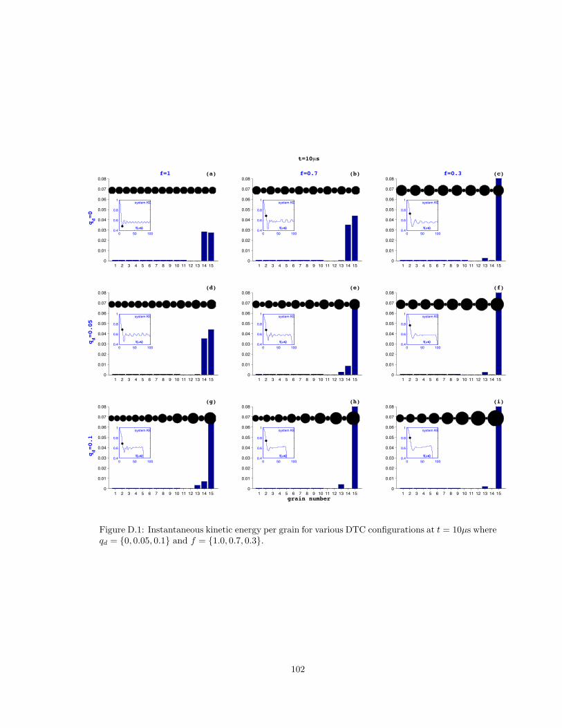
1 2 + 4 ( % - & , 10 11 12 1+ 14 1(0

0"01

0"02

0"0+

0"04

0"0(

0"0%

0"0-

0"0&

qd=0

(a) f=1

0 (0 1000"4

0"%

0"&

1

t(µs)

system KE

1 2 + 4 ( % - & , 10 11 12 1+ 14 1(0

0"01

0"02

0"0+

0"04

0"0(

0"0%

0"0-

0"0&(b) f=0.7

t=10µs

0 (0 1000"4

0"%

0"&

1

t(µs)

system KE

1 2 + 4 ( % - & , 10 11 12 1+ 14 1(0

0"01

0"02

0"0+

0"04

0"0(

0"0%

0"0-

0"0&(c) f=0.3

0 (0 1000"4

0"%

0"&

1

t(µs)

system KE

1 2 + 4 ( % - & , 10 11 12 1+ 14 1(0

0"01

0"02

0"0+

0"04

0"0(

0"0%

0"0-

0"0&

qd=0.05

(d)

0 (0 1000"4

0"%

0"&

1

t(µs)

system KE

1 2 + 4 ( % - & , 10 11 12 1+ 14 1(0

0"01

0"02

0"0+

0"04

0"0(

0"0%

0"0-

0"0&(e)

0 (0 1000"4

0"%

0"&

1

t(µs)

system KE

1 2 + 4 ( % - & , 10 11 12 1+ 14 1(0

0"01

0"02

0"0+

0"04

0"0(

0"0%

0"0-

0"0&(f)

0 (0 1000"4

0"%

0"&

1

t(µs)

system KE

1 2 + 4 ( % - & , 10 11 12 1+ 14 1(0

0"01

0"02

0"0+

0"04

0"0(

0"0%

0"0-

0"0&

qd=0.1

(g)

0 (0 1000"4

0"%

0"&

1

t(µs)

system KE

1 2 + 4 ( % - & , 10 11 12 1+ 14 1(0

0"01

0"02

0"0+

0"04

0"0(

0"0%

0"0-

0"0&

grain number

(h)

0 (0 1000"4

0"%

0"&

1

t(µs)

system KE

1 2 + 4 ( % - & , 10 11 12 1+ 14 1(0

0"01

0"02

0"0+

0"04

0"0(

0"0%

0"0-

0"0&(i)

0 (0 1000"4

0"%

0"&

1

t(µs)

system KE

Figure D.1: Instantaneous kinetic energy per grain for various DTC configurations at t = 10µs whereqd = {0, 0.05, 0.1} and f = {1.0, 0.7, 0.3}.

102

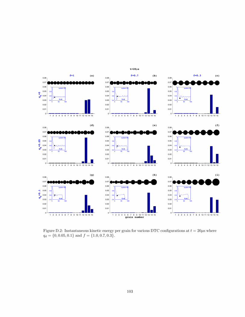
1 2 + 4 ( % - & , 10 11 12 1+ 14 1(0

0"01

0"02

0"0+

0"04

0"0(

0"0%

0"0-

0"0&

qd=0

(a) f=1

0 (0 1000"4

0"%

0"&

1

t(µs)

system KE

1 2 + 4 ( % - & , 10 11 12 1+ 14 1(0

0"01

0"02

0"0+

0"04

0"0(

0"0%

0"0-

0"0&(b) f=0.7

t=20µs

0 (0 1000"4

0"%

0"&

1

t(µs)

system KE

1 2 + 4 ( % - & , 10 11 12 1+ 14 1(0

0"01

0"02

0"0+

0"04

0"0(

0"0%

0"0-

0"0&(c) f=0.3

0 (0 1000"4

0"%

0"&

1

t(µs)

system KE

1 2 + 4 ( % - & , 10 11 12 1+ 14 1(0

0"01

0"02

0"0+

0"04

0"0(

0"0%

0"0-

0"0&

qd=0.05

(d)

0 (0 1000"4

0"%

0"&

1

t(µs)

system KE

1 2 + 4 ( % - & , 10 11 12 1+ 14 1(0

0"01

0"02

0"0+

0"04

0"0(

0"0%

0"0-

0"0&(e)

0 (0 1000"4

0"%

0"&

1

t(µs)

system KE

1 2 + 4 ( % - & , 10 11 12 1+ 14 1(0

0"01

0"02

0"0+

0"04

0"0(

0"0%

0"0-

0"0&(f)

0 (0 1000"4

0"%

0"&

1

t(µs)

system KE

1 2 + 4 ( % - & , 10 11 12 1+ 14 1(0

0"01

0"02

0"0+

0"04

0"0(

0"0%

0"0-

0"0&

qd=0.1

(g)

0 (0 1000"4

0"%

0"&

1

t(µs)

system KE

1 2 + 4 ( % - & , 10 11 12 1+ 14 1(0

0"01

0"02

0"0+

0"04

0"0(

0"0%

0"0-

0"0&

grain number

(h)

0 (0 1000"4

0"%

0"&

1

t(µs)

system KE

1 2 + 4 ( % - & , 10 11 12 1+ 14 1(0

0"01

0"02

0"0+

0"04

0"0(

0"0%

0"0-

0"0&(i)

0 (0 1000"4

0"%

0"&

1

t(µs)

system KE


103

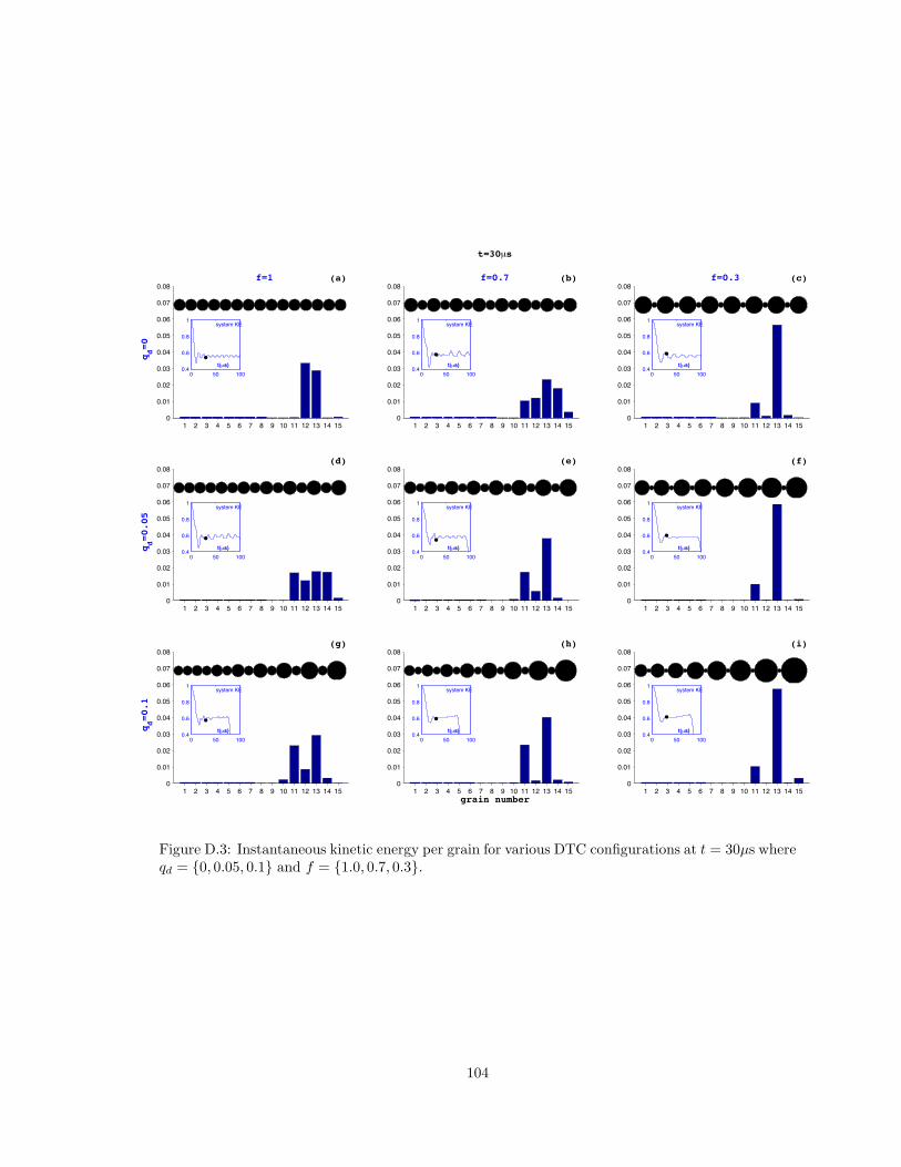
1 2 + 4 ( % - & , 10 11 12 1+ 14 1(0

0"01

0"02

0"0+

0"04

0"0(

0"0%

0"0-

0"0&

qd=0

(a) f=1

0 (0 1000"4

0"%

0"&

1

t(µs)

system KE

1 2 + 4 ( % - & , 10 11 12 1+ 14 1(0

0"01

0"02

0"0+

0"04

0"0(

0"0%

0"0-

0"0&(b) f=0.7

t=30µs

0 (0 1000"4

0"%

0"&

1

t(µs)

system KE

1 2 + 4 ( % - & , 10 11 12 1+ 14 1(0

0"01

0"02

0"0+

0"04

0"0(

0"0%

0"0-

0"0&(c) f=0.3

0 (0 1000"4

0"%

0"&

1

t(µs)

system KE

1 2 + 4 ( % - & , 10 11 12 1+ 14 1(0

0"01

0"02

0"0+

0"04

0"0(

0"0%

0"0-

0"0&

qd=0.05

(d)

0 (0 1000"4

0"%

0"&

1

t(µs)

system KE

1 2 + 4 ( % - & , 10 11 12 1+ 14 1(0

0"01

0"02

0"0+

0"04

0"0(

0"0%

0"0-

0"0&(e)

0 (0 1000"4

0"%

0"&

1

t(µs)

system KE

1 2 + 4 ( % - & , 10 11 12 1+ 14 1(0

0"01

0"02

0"0+

0"04

0"0(

0"0%

0"0-

0"0&(f)

0 (0 1000"4

0"%

0"&

1

t(µs)

system KE

1 2 + 4 ( % - & , 10 11 12 1+ 14 1(0

0"01

0"02

0"0+

0"04

0"0(

0"0%

0"0-

0"0&

qd=0.1

(g)

0 (0 1000"4

0"%

0"&

1

t(µs)

system KE

1 2 + 4 ( % - & , 10 11 12 1+ 14 1(0

0"01

0"02

0"0+

0"04

0"0(

0"0%

0"0-

0"0&

grain number

(h)

0 (0 1000"4

0"%

0"&

1

t(µs)

system KE

1 2 + 4 ( % - & , 10 11 12 1+ 14 1(0

0"01

0"02

0"0+

0"04

0"0(

0"0%

0"0-

0"0&(i)

0 (0 1000"4

0"%

0"&

1

t(µs)

system KE


104

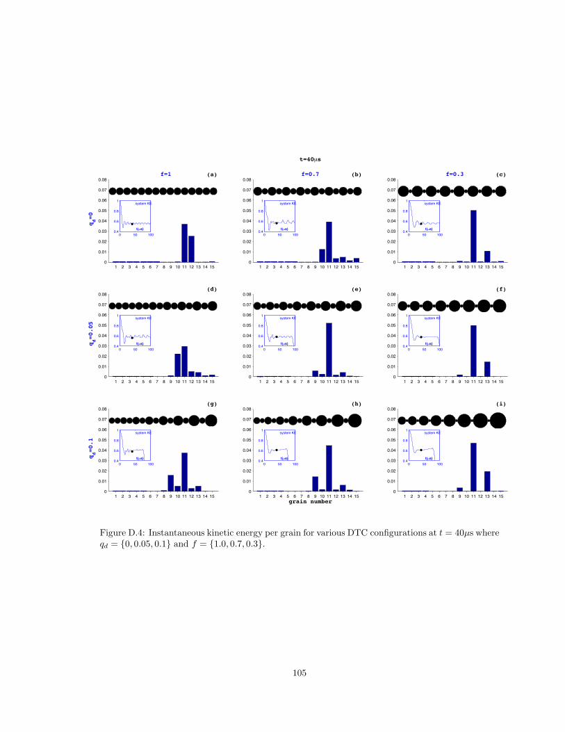
1 2 + 4 ( % - & , 10 11 12 1+ 14 1(0

0"01

0"02

0"0+

0"04

0"0(

0"0%

0"0-

0"0&

qd=0

(a) f=1

0 (0 1000"4

0"%

0"&

1

t(µs)

system KE

1 2 + 4 ( % - & , 10 11 12 1+ 14 1(0

0"01

0"02

0"0+

0"04

0"0(

0"0%

0"0-

0"0&(b) f=0.7

t=40µs

0 (0 1000"4

0"%

0"&

1

t(µs)

system KE

1 2 + 4 ( % - & , 10 11 12 1+ 14 1(0

0"01

0"02

0"0+

0"04

0"0(

0"0%

0"0-

0"0&(c) f=0.3

0 (0 1000"4

0"%

0"&

1

t(µs)

system KE

1 2 + 4 ( % - & , 10 11 12 1+ 14 1(0

0"01

0"02

0"0+

0"04

0"0(

0"0%

0"0-

0"0&

qd=0.05

(d)

0 (0 1000"4

0"%

0"&

1

t(µs)

system KE

1 2 + 4 ( % - & , 10 11 12 1+ 14 1(0

0"01

0"02

0"0+

0"04

0"0(

0"0%

0"0-

0"0&(e)

0 (0 1000"4

0"%

0"&

1

t(µs)

system KE

1 2 + 4 ( % - & , 10 11 12 1+ 14 1(0

0"01

0"02

0"0+

0"04

0"0(

0"0%

0"0-

0"0&(f)

0 (0 1000"4

0"%

0"&

1

t(µs)

system KE

1 2 + 4 ( % - & , 10 11 12 1+ 14 1(0

0"01

0"02

0"0+

0"04

0"0(

0"0%

0"0-

0"0&

qd=0.1

(g)

0 (0 1000"4

0"%

0"&

1

t(µs)

system KE

1 2 + 4 ( % - & , 10 11 12 1+ 14 1(0

0"01

0"02

0"0+

0"04

0"0(

0"0%

0"0-

0"0&

grain number

(h)

0 (0 1000"4

0"%

0"&

1

t(µs)

system KE

1 2 + 4 ( % - & , 10 11 12 1+ 14 1(0

0"01

0"02

0"0+

0"04

0"0(

0"0%

0"0-

0"0&(i)

0 (0 1000"4

0"%

0"&

1

t(µs)

system KE


105

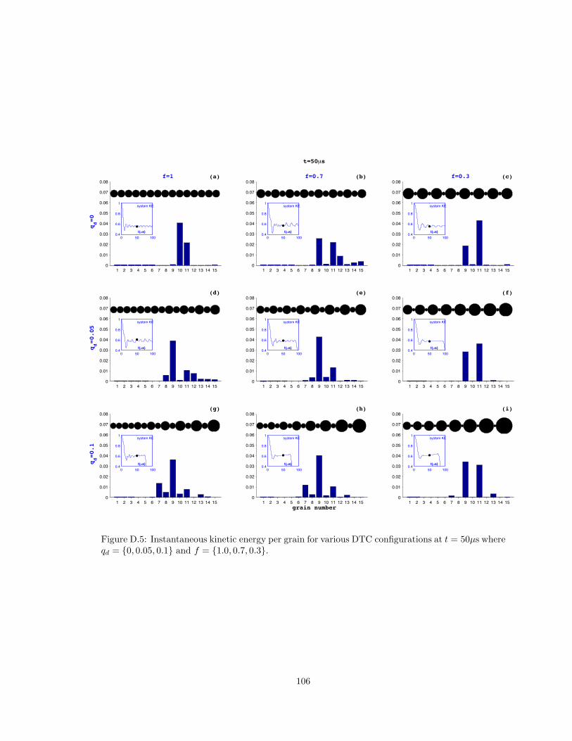
1 2 + 4 ( % - & , 10 11 12 1+ 14 1(0

0"01

0"02

0"0+

0"04

0"0(

0"0%

0"0-

0"0&

qd=0

(a) f=1

0 (0 1000"4

0"%

0"&

1

t(µs)

system KE

1 2 + 4 ( % - & , 10 11 12 1+ 14 1(0

0"01

0"02

0"0+

0"04

0"0(

0"0%

0"0-

0"0&(b) f=0.7

t=50µs

0 (0 1000"4

0"%

0"&

1

t(µs)

system KE

1 2 + 4 ( % - & , 10 11 12 1+ 14 1(0

0"01

0"02

0"0+

0"04

0"0(

0"0%

0"0-

0"0&(c) f=0.3

0 (0 1000"4

0"%

0"&

1

t(µs)

system KE

1 2 + 4 ( % - & , 10 11 12 1+ 14 1(0

0"01

0"02

0"0+

0"04

0"0(

0"0%

0"0-

0"0&

qd=0.05

(d)

0 (0 1000"4

0"%

0"&

1

t(µs)

system KE

1 2 + 4 ( % - & , 10 11 12 1+ 14 1(0

0"01

0"02

0"0+

0"04

0"0(

0"0%

0"0-

0"0&(e)

0 (0 1000"4

0"%

0"&

1

t(µs)

system KE

1 2 + 4 ( % - & , 10 11 12 1+ 14 1(0

0"01

0"02

0"0+

0"04

0"0(

0"0%

0"0-

0"0&(f)

0 (0 1000"4

0"%

0"&

1

t(µs)

system KE

1 2 + 4 ( % - & , 10 11 12 1+ 14 1(0

0"01

0"02

0"0+

0"04

0"0(

0"0%

0"0-

0"0&

qd=0.1

(g)

0 (0 1000"4

0"%

0"&

1

t(µs)

system KE

1 2 + 4 ( % - & , 10 11 12 1+ 14 1(0

0"01

0"02

0"0+

0"04

0"0(

0"0%

0"0-

0"0&

grain number

(h)

0 (0 1000"4

0"%

0"&

1

t(µs)

system KE

1 2 + 4 ( % - & , 10 11 12 1+ 14 1(0

0"01

0"02

0"0+

0"04

0"0(

0"0%

0"0-

0"0&(i)

0 (0 1000"4

0"%

0"&

1

t(µs)

system KE


106

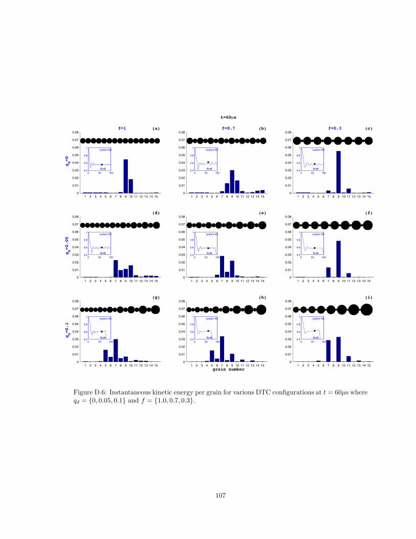
1 2 + 4 ( % - & , 10 11 12 1+ 14 1(0

0"01

0"02

0"0+

0"04

0"0(

0"0%

0"0-

0"0&

qd=0

(a) f=1

0 (0 1000"4

0"%

0"&

1

t(µs)

system KE

1 2 + 4 ( % - & , 10 11 12 1+ 14 1(0

0"01

0"02

0"0+

0"04

0"0(

0"0%

0"0-

0"0&(b) f=0.7

t=60µs

0 (0 1000"4

0"%

0"&

1

t(µs)

system KE

1 2 + 4 ( % - & , 10 11 12 1+ 14 1(0

0"01

0"02

0"0+

0"04

0"0(

0"0%

0"0-

0"0&(c) f=0.3

0 (0 1000"4

0"%

0"&

1

t(µs)

system KE

1 2 + 4 ( % - & , 10 11 12 1+ 14 1(0

0"01

0"02

0"0+

0"04

0"0(

0"0%

0"0-

0"0&

qd=0.05

(d)

0 (0 1000"4

0"%

0"&

1

t(µs)

system KE

1 2 + 4 ( % - & , 10 11 12 1+ 14 1(0

0"01

0"02

0"0+

0"04

0"0(

0"0%

0"0-

0"0&(e)

0 (0 1000"4

0"%

0"&

1

t(µs)

system KE

1 2 + 4 ( % - & , 10 11 12 1+ 14 1(0

0"01

0"02

0"0+

0"04

0"0(

0"0%

0"0-

0"0&(f)

0 (0 1000"4

0"%

0"&

1

t(µs)

system KE

1 2 + 4 ( % - & , 10 11 12 1+ 14 1(0

0"01

0"02

0"0+

0"04

0"0(

0"0%

0"0-

0"0&

qd=0.1

(g)

0 (0 1000"4

0"%

0"&

1

t(µs)

system KE

1 2 + 4 ( % - & , 10 11 12 1+ 14 1(0

0"01

0"02

0"0+

0"04

0"0(

0"0%

0"0-

0"0&

grain number

(h)

0 (0 1000"4

0"%

0"&

1

t(µs)

system KE

1 2 + 4 ( % - & , 10 11 12 1+ 14 1(0

0"01

0"02

0"0+

0"04

0"0(

0"0%

0"0-

0"0&(i)

0 (0 1000"4

0"%

0"&

1

t(µs)

system KE


107

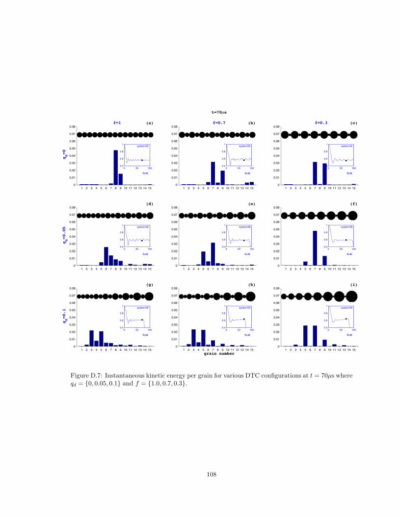
1 2 + 4 ( % - & , 10 11 12 1+ 14 1(0

0"01

0"02

0"0+

0"04

0"0(

0"0%

0"0-

0"0&

qd=0

(a) f=1

0 (0 1000"4

0"%

0"&

1

t(µs)

system KE

1 2 + 4 ( % - & , 10 11 12 1+ 14 1(0

0"01

0"02

0"0+

0"04

0"0(

0"0%

0"0-

0"0&(b) f=0.7

t=70µs

0 (0 1000"4

0"%

0"&

1

t(µs)

system KE

1 2 + 4 ( % - & , 10 11 12 1+ 14 1(0

0"01

0"02

0"0+

0"04

0"0(

0"0%

0"0-

0"0&(c) f=0.3

0 (0 1000"4

0"%

0"&

1

t(µs)

system KE

1 2 + 4 ( % - & , 10 11 12 1+ 14 1(0

0"01

0"02

0"0+

0"04

0"0(

0"0%

0"0-

0"0&

qd=0.05

(d)

0 (0 1000"4

0"%

0"&

1

t(µs)

system KE

1 2 + 4 ( % - & , 10 11 12 1+ 14 1(0

0"01

0"02

0"0+

0"04

0"0(

0"0%

0"0-

0"0&(e)

0 (0 1000"4

0"%

0"&

1

t(µs)

system KE

1 2 + 4 ( % - & , 10 11 12 1+ 14 1(0

0"01

0"02

0"0+

0"04

0"0(

0"0%

0"0-

0"0&(f)

0 (0 1000"4

0"%

0"&

1

t(µs)

system KE

1 2 + 4 ( % - & , 10 11 12 1+ 14 1(0

0"01

0"02

0"0+

0"04

0"0(

0"0%

0"0-

0"0&

qd=0.1

(g)

0 (0 1000"4

0"%

0"&

1

t(µs)

system KE

1 2 + 4 ( % - & , 10 11 12 1+ 14 1(0

0"01

0"02

0"0+

0"04

0"0(

0"0%

0"0-

0"0&

grain number

(h)

0 (0 1000"4

0"%

0"&

1

t(µs)

system KE

1 2 + 4 ( % - & , 10 11 12 1+ 14 1(0

0"01

0"02

0"0+

0"04

0"0(

0"0%

0"0-

0"0&(i)

0 (0 1000"4

0"%

0"&

1

t(µs)

system KE


108

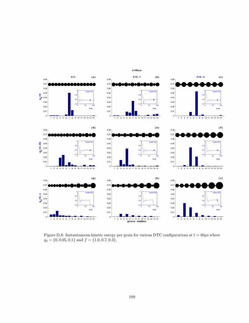
1 2 + 4 ( % - & , 10 11 12 1+ 14 1(0

0"01

0"02

0"0+

0"04

0"0(

0"0%

0"0-

0"0&

qd=0

(a) f=1

0 (0 1000"4

0"%

0"&

1

t(µs)

system KE

1 2 + 4 ( % - & , 10 11 12 1+ 14 1(0

0"01

0"02

0"0+

0"04

0"0(

0"0%

0"0-

0"0&(b) f=0.7

t=80µs

0 (0 1000"4

0"%

0"&

1

t(µs)

system KE

1 2 + 4 ( % - & , 10 11 12 1+ 14 1(0

0"01

0"02

0"0+

0"04

0"0(

0"0%

0"0-

0"0&(c) f=0.3

0 (0 1000"4

0"%

0"&

1

t(µs)

system KE

1 2 + 4 ( % - & , 10 11 12 1+ 14 1(0

0"01

0"02

0"0+

0"04

0"0(

0"0%

0"0-

0"0&

qd=0.05

(d)

0 (0 1000"4

0"%

0"&

1

t(µs)

system KE

1 2 + 4 ( % - & , 10 11 12 1+ 14 1(0

0"01

0"02

0"0+

0"04

0"0(

0"0%

0"0-

0"0&(e)

0 (0 1000"4

0"%

0"&

1

t(µs)

system KE

1 2 + 4 ( % - & , 10 11 12 1+ 14 1(0

0"01

0"02

0"0+

0"04

0"0(

0"0%

0"0-

0"0&(f)

0 (0 1000"4

0"%

0"&

1

t(µs)

system KE

1 2 + 4 ( % - & , 10 11 12 1+ 14 1(0

0"01

0"02

0"0+

0"04

0"0(

0"0%

0"0-

0"0&

qd=0.1

(g)

0 (0 1000"4

0"%

0"&

1

t(µs)

system KE

1 2 + 4 ( % - & , 10 11 12 1+ 14 1(0

0"01

0"02

0"0+

0"04

0"0(

0"0%

0"0-

0"0&

grain number

(h)

0 (0 1000"4

0"%

0"&

1

t(µs)

system KE

1 2 + 4 ( % - & , 10 11 12 1+ 14 1(0

0"01

0"02

0"0+

0"04

0"0(

0"0%

0"0-

0"0&(i)

0 (0 1000"4

0"%

0"&

1

t(µs)

system KE


109

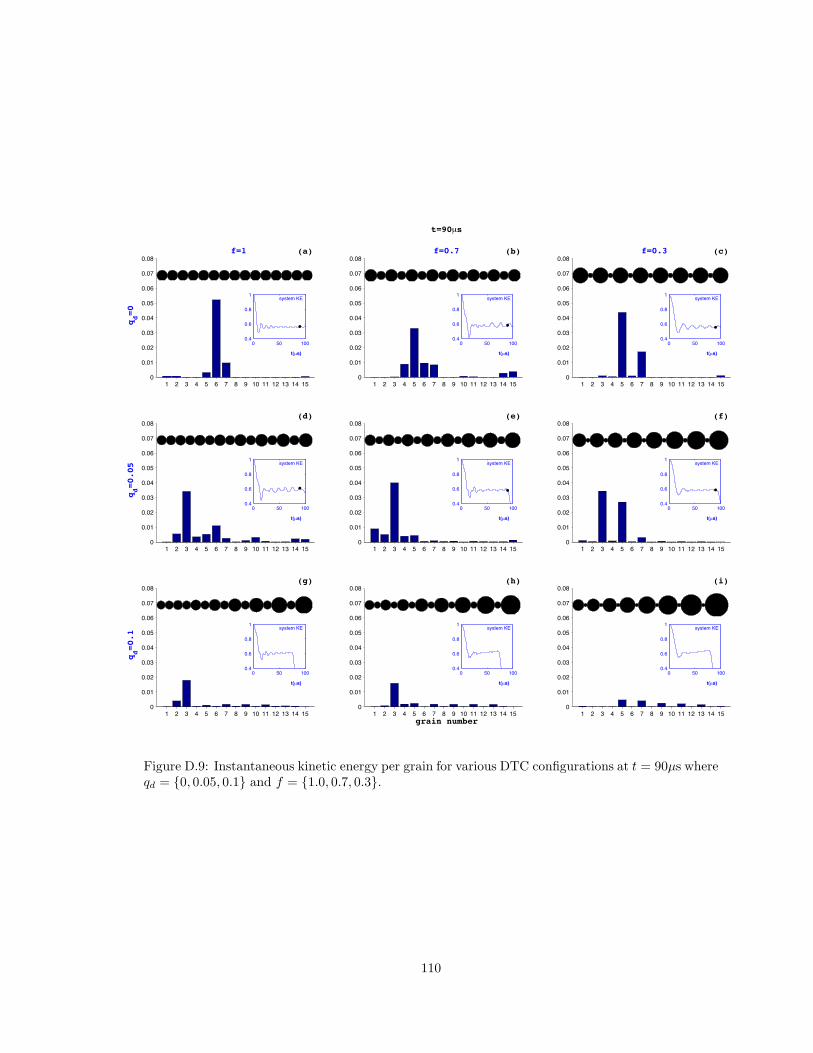
1 2 + 4 ( % - & , 10 11 12 1+ 14 1(0

0"01

0"02

0"0+

0"04

0"0(

0"0%

0"0-

0"0&

qd=0

(a) f=1

0 (0 1000"4

0"%

0"&

1

t(µs)

system KE

1 2 + 4 ( % - & , 10 11 12 1+ 14 1(0

0"01

0"02

0"0+

0"04

0"0(

0"0%

0"0-

0"0&(b) f=0.7

t=90µs

0 (0 1000"4

0"%

0"&

1

t(µs)

system KE

1 2 + 4 ( % - & , 10 11 12 1+ 14 1(0

0"01

0"02

0"0+

0"04

0"0(

0"0%

0"0-

0"0&(c) f=0.3

0 (0 1000"4

0"%

0"&

1

t(µs)

system KE

1 2 + 4 ( % - & , 10 11 12 1+ 14 1(0

0"01

0"02

0"0+

0"04

0"0(

0"0%

0"0-

0"0&

qd=0.05

(d)

0 (0 1000"4

0"%

0"&

1

t(µs)

system KE

1 2 + 4 ( % - & , 10 11 12 1+ 14 1(0

0"01

0"02

0"0+

0"04

0"0(

0"0%

0"0-

0"0&(e)

0 (0 1000"4

0"%

0"&

1

t(µs)

system KE

1 2 + 4 ( % - & , 10 11 12 1+ 14 1(0

0"01

0"02

0"0+

0"04

0"0(

0"0%

0"0-

0"0&(f)

0 (0 1000"4

0"%

0"&

1

t(µs)

system KE

1 2 + 4 ( % - & , 10 11 12 1+ 14 1(0

0"01

0"02

0"0+

0"04

0"0(

0"0%

0"0-

0"0&

qd=0.1

(g)

0 (0 1000"4

0"%

0"&

1

t(µs)

system KE

1 2 + 4 ( % - & , 10 11 12 1+ 14 1(0

0"01

0"02

0"0+

0"04

0"0(

0"0%

0"0-

0"0&

grain number

(h)

0 (0 1000"4

0"%

0"&

1

t(µs)

system KE

1 2 + 4 ( % - & , 10 11 12 1+ 14 1(0

0"01

0"02

0"0+

0"04

0"0(

0"0%

0"0-

0"0&(i)

0 (0 1000"4

0"%

0"&

1

t(µs)

system KE


110

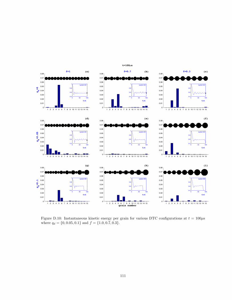
1 2 + 4 ( % - & , 10 11 12 1+ 14 1(0

0"01

0"02

0"0+

0"04

0"0(

0"0%

0"0-

0"0&

qd=0

(a) f=1

0 (0 1000"4

0"%

0"&

1

t(µs)

system KE

1 2 + 4 ( % - & , 10 11 12 1+ 14 1(0

0"01

0"02

0"0+

0"04

0"0(

0"0%

0"0-

0"0&(b) f=0.7

t=100µs

0 (0 1000"4

0"%

0"&

1

t(µs)

system KE

1 2 + 4 ( % - & , 10 11 12 1+ 14 1(0

0"01

0"02

0"0+

0"04

0"0(

0"0%

0"0-

0"0&(c) f=0.3

0 (0 1000"4

0"%

0"&

1

t(µs)

system KE

1 2 + 4 ( % - & , 10 11 12 1+ 14 1(0

0"01

0"02

0"0+

0"04

0"0(

0"0%

0"0-

0"0&

qd=0.05

(d)

0 (0 1000"4

0"%

0"&

1

t(µs)

system KE

1 2 + 4 ( % - & , 10 11 12 1+ 14 1(0

0"01

0"02

0"0+

0"04

0"0(

0"0%

0"0-

0"0&(e)

0 (0 1000"4

0"%

0"&

1

t(µs)

system KE

1 2 + 4 ( % - & , 10 11 12 1+ 14 1(0

0"01

0"02

0"0+

0"04

0"0(

0"0%

0"0-

0"0&(f)

0 (0 1000"4

0"%

0"&

1

t(µs)

system KE

1 2 + 4 ( % - & , 10 11 12 1+ 14 1(0

0"01

0"02

0"0+

0"04

0"0(

0"0%

0"0-

0"0&

qd=0.1

(g)

0 (0 1000"4

0"%

0"&

1

t(µs)

system KE

1 2 + 4 ( % - & , 10 11 12 1+ 14 1(0

0"01

0"02

0"0+

0"04

0"0(

0"0%

0"0-

0"0&

grain number

(h)

0 (0 1000"4

0"%

0"&

1

t(µs)

system KE

1 2 + 4 ( % - & , 10 11 12 1+ 14 1(0

0"01

0"02

0"0+

0"04

0"0(

0"0%

0"0-

0"0&(i)

0 (0 1000"4

0"%

0"&

1

t(µs)

system KE

Figure D.10: Instantaneous kinetic energy per grain for various DTC configurations at t = 100µswhere qd = {0, 0.05, 0.1} and f = {1.0, 0.7, 0.3}.

111

Appendix E

Normalization

Normalization has posed some challenges in trying to properly assess the absorption quality of a

simple tapered chain (STC). Proper normalization schemes will help the architect better determine

which STC is best for which application. Recall that the goal is to measure the energy at the last

grain versus the energy put into the system by the first. In general, the functional form will stay the

same regardless of the strategy and adjustments in the normalization will simply scale the kinetic

energy (KE) surface. In some cases, the output force of each chain is based on the maximum value

felt by any possible chain under consideration (i.e. monodisperse and no energy loss)1. This gives a

measure of how one chain is better than another.

In this communication, we have chosen to form the ratio based on the output KE and force

felt by each specific chain. This serves to grade the individual e!ectiveness of any chain without

reference to another. In choosing a peak value with this method, one could identify either when

the impulse first hits the last grain or look for the absolute maximum peak whenever it may occur.

We have chosen to use the former for several reasons. First, it ignores the complexity of nonlinear

reverberations which can lead to large peaks at unpredictable times. Second, we argue that this is

just as realistic as selecting the maximum value anywhere in the time spectrum.

It turns out that in most cases, the absolute maximum is the first peak. There are special cases

where the maximum may occur at later times and this needs to be investigated further. In figure 2.5

(in the body of the report) for q = 0.1, for example, we see the striking occurrence of the secondary

pulse about 225 µs being much stronger than the initial arrival at 35 µs. This is one of those

instances that disagrees with the way we choose to normalize our KE surfaces. We have investigated

this particular case further without including extraneous plots and report the following observations.

The e!ect exists for N = 15 $ 20 for constant ". When N = 20 is held fixed and restitution is

increased, the peak KE once again occurs for the first arrival of the pulse. As q increases, so do the

number of collisions and the requisite energy loss (since " )= 0). Therefore, it is less likely to find a

global peak later in the simulation. The situation is further complicated by the interplay between q

1Pfannes, J. Energy propagation in granular chains M.S. Thesis, SUNY Bu!alo, May 2003.

112

and ".

113

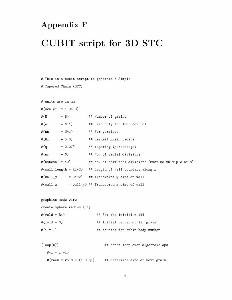
Appendix F

CUBIT script for 3D STC

# This is a cubit script to generate a Simple

# Tapered Chain (STC).

# units are in mm

#{scalef = 1.0e-3}

#{N = 5} ## Number of grains

#{n = N-1} ## used only for loop control

#{nn = N+1} ## For vertices

#{Ri = 5.0} ## Largest grain radius

#{q = 0.07} ## tapering (percentage)

#{nr = 6} ## No. of radial divisions

#{ntheta = 40} ## No. of azimuthal divisions (must be multiple of 8)

#{wall_length = Ri*2} ## Length of wall boundary along x

#{wall_y = Ri*2} ## Transverse y size of wall

#{wall_z = wall_y} ## Transverse z size of wall

graphics mode wire

create sphere radius {Ri}

#{rold = Ri} ## Set the initial r_old

#{xold = 0} ## Initial center of 1st grain

#{i = 1} ## counter for cubit body number

{loop(n)} ## can’t loop over algebraic ops

#{i = i +1}

#{rnew = rold * (1.0-q)} ## determine size of next grain

114

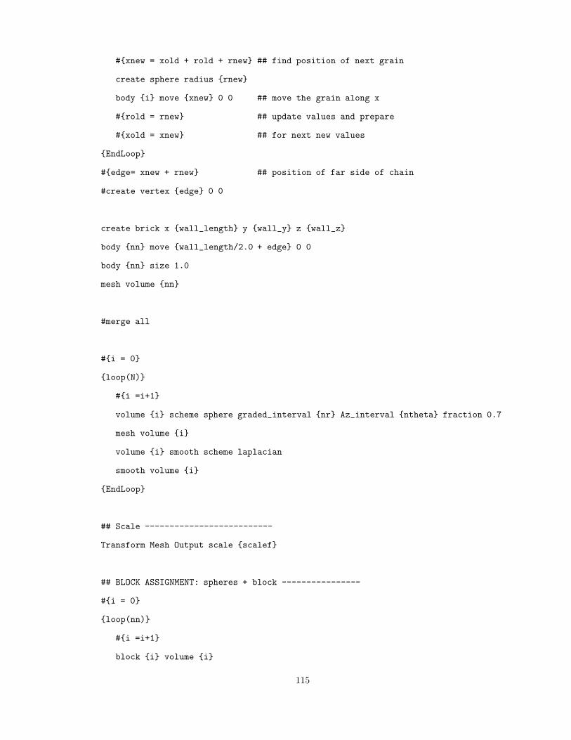
#{xnew = xold + rold + rnew} ## find position of next grain

create sphere radius {rnew}

body {i} move {xnew} 0 0 ## move the grain along x

#{rold = rnew} ## update values and prepare

#{xold = xnew} ## for next new values

{EndLoop}

#{edge= xnew + rnew} ## position of far side of chain

#create vertex {edge} 0 0

create brick x {wall_length} y {wall_y} z {wall_z}

body {nn} move {wall_length/2.0 + edge} 0 0

body {nn} size 1.0

mesh volume {nn}

#merge all

#{i = 0}

{loop(N)}

#{i =i+1}

volume {i} scheme sphere graded_interval {nr} Az_interval {ntheta} fraction 0.7

mesh volume {i}

volume {i} smooth scheme laplacian

smooth volume {i}

{EndLoop}

## Scale --------------------------

Transform Mesh Output scale {scalef}

## BLOCK ASSIGNMENT: spheres + block ----------------

#{i = 0}

{loop(nn)}

#{i =i+1}

block {i} volume {i}

115

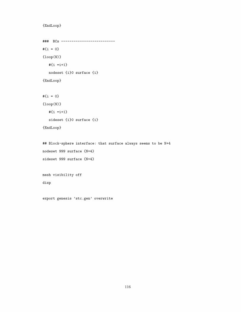
{EndLoop}

### BCs --------------------------

#{i = 0}

{loop(N)}

#{i =i+1}

nodeset {i}0 surface {i}

{EndLoop}

#{i = 0}

{loop(N)}

#{i =i+1}

sideset {i}0 surface {i}

{EndLoop}

## Block-sphere interface: that surface always seems to be N+4

nodeset 999 surface {N+4}

sideset 999 surface {N+4}

mesh visibility off

disp

export genesis ’stc.gen’ overwrite

116

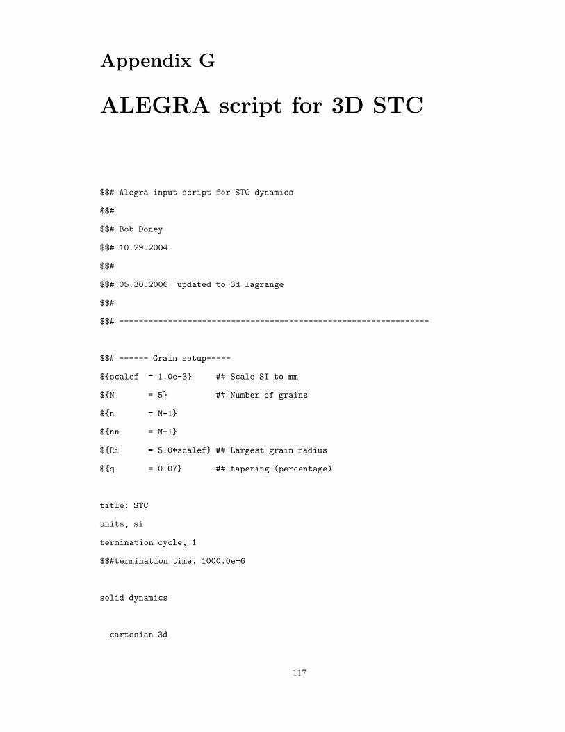
Appendix G

ALEGRA script for 3D STC

$$# Alegra input script for STC dynamics

$$#

$$# Bob Doney

$$# 10.29.2004

$$#

$$# 05.30.2006 updated to 3d lagrange

$$#

$$# ----------------------------------------------------------------

$$# ------ Grain setup-----

${scalef = 1.0e-3} ## Scale SI to mm

${N = 5} ## Number of grains

${n = N-1}

${nn = N+1}

${Ri = 5.0*scalef} ## Largest grain radius

${q = 0.07} ## tapering (percentage)

title: STC

units, si

termination cycle, 1

$$#termination time, 1000.0e-6

solid dynamics

cartesian 3d

117

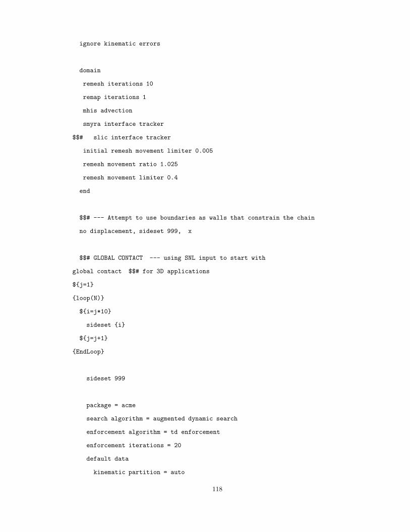
ignore kinematic errors

domain

remesh iterations 10

remap iterations 1

mhis advection

smyra interface tracker

$$# slic interface tracker

initial remesh movement limiter 0.005

remesh movement ratio 1.025

remesh movement limiter 0.4

end

$$# --- Attempt to use boundaries as walls that constrain the chain

no displacement, sideset 999, x

$$# GLOBAL CONTACT --- using SNL input to start with

global contact $$# for 3D applications

${j=1}

{loop(N)}

${i=j*10}

sideset {i}

${j=j+1}

{EndLoop}

sideset 999

package = acme

search algorithm = augmented dynamic search

enforcement algorithm = td enforcement

enforcement iterations = 20

default data

kinematic partition = auto

118

friction model id = 1

search normal tolerance = .0001

search tangential tolerance = .0001

end

friction model 1 frictionless

$no subkeywords

end

end

initial block velocity: block 1, x 500.0

maximum initial time step 1.0e-9

$$# TRACER PARTICLES

tracer points

lagrangian tracer 1 x=0 y=0 z=0 $$# Initial one at origin

${rold = Ri} $$# Set the initial r_old

${xold = 0} $$# Initial center of 1st grain

${i=0}

$$# Center of spheres

{loop(n)} $$# N-1

${i = i+1}

${rnew = rold * (1.0-q)} $$# determine radius of next grain

${xnew = xold + rold + rnew}

lagrangian tracer {i+1} x = {xnew} y=0 z=0

${rold = rnew} $$# update values and prepare

${xold = xnew} $$# for next new values

{EndLoop}

$$# Wall-last sphere interface

119

lagrangian tracer {nn} x= {xnew+rnew} y=0 z=0

end $$# End tracer section

$$# MESH

${i=0}

{loop(nn)}

${i=i+1}

block {i}

LAGRANGIAN MESH

material {i}

# hourglass control {i}

end

{EndLoop}

end $$# -- end physics --

$$# ----------------------------------------------------------------

$$# --- PLOTTING ---

$$#double precision exodus

emit output, time interval=1.e-6

emit plot, time interval=1.e-6

emit hisplt, time interval=0.2e-6

plot variables

no underscores

velocity

density

density,avg

temperature

temperature, avg

120

energy

stress

stress, avg

end

history plot variables

no material globals

end

$$# ----------------------------------------------------------------

$$# --- MATERIALS

${i=0}

{loop(nn)}

${i=i+1}

material {i} $$# Copper spheres

model = 100

end

{EndLoop}

$--- ELASTIC-PLASTIC ---

model 100 cth elastic plastic

eos model = 11

yield model = 12

end

$$# EOS

model 11, keos sesame

feos = ’sesame’

neos = 3320

clip = 1.0

end

121

$$# YIELD

model 12 johnson cook ep

matlabel = ’COPPER’

end

exit

122

References

1. Materials research society symposium proceedings: The granular state. In The Granular State(San Francisco, 2000), S. Sen and M. Hunt, Eds., vol. 627, Materials Research Society.

2. Agui, J. To be submitted .

3. Allen, M., and Tildesley, D. Computer Simulation of Liquids. Oxford. Clarendon, 1987.

4. Ball, J. He died with his best buddy, citizen times, March 19 2006.

5. Barnes, G. Study of collisions part i: Survey of the periodical literature. American Journalof Physics 26 (1958), 5–8.

6. Barnes, G. Study of collisions part ii: Survey of the textbooks. American Journal of Physics26 (1958), 9–12.

7. Batteh, J., and Powell, J. Shock propagation in the one-dimensional lattice at nonzeroinitial temperature. Journal of Applied Physics 49, 7 (1978), 3933–3940.

8. Bell, R., and Hertel, E. An improved material interface reconstruction algorithm foreulerian codes, 1992.

9. Bhatnagar, P. Nonlinear Waves in One-dimensional Dispersive Systems. Clarendon Press,Oxford, 1979.

10. Bocchieri, P., Scotti, A., Bearzi, B., and Loinger, A. Anharmonic chain with lennard-jones interaction. Physical Review A 2, 5 (1970), 2013.

11. Bokor, A., and Leventhall, H. The measurement of initial impact velocity and contacttime. Journal of Physics D: Applied Physics 4 (1971), 160.

12. Boyle, J. Wnc honors ‘fallen heroes’, citizen times, March 22 2006.

13. Brown, K., Summers, R., Glass, M., Gullerud, A., Heinstein, M., and Jones, R.Acme: Algorithms for contact in a multiphysics environment api version 1.0, 2001.

14. Bruck, H. A one-dimensional model for designing functionally graded materials to managestress waves. International Journal of Solids and Structures 37 (2001), 6383–6395.

15. Burgers, J. Mathematical examples illustrating relations occuring in the theory of turbulentfluid motion. Trans. R. Neth. Acad. Sci. 17 (1939), 1–53.

16. Carroll, S., Drake, R., Hensinger, D., Luchini, C., Petney, S., Robbins, J., Robin-son, A., Summers., R., Voth, T., Weirs, V., Wong, M., Brunner, T., Garasi, C.,Haill, T., and Hanshaw, H.L., M. T. Alegra: Version 4.6 (revised), 2005.

17. CEI. http://www.ensight.com, 2005.

123

18. Chhabildas, L., Konrad, C., Mosher, D., Reinhard, W., Duggins, B., Trucano, T.,Summers, R., and Peery, J. A methodology to validate 3d arbitrary lagrangian euleriancodes with applications to alegra. International Journal of Impact Engineering 23, 1 (1999),101–112.

19. Coaplen, J., Stronge, W., and Ravani, B. Work equivalent composite coe"cient ofrestitution. International Journal of Impact Engineering 30 (2004), 581–591.

20. Coste, C., Falcon, E., and Fauve, S. Solitary waves in a chain of beads under hertzcontact. Physical Review E 56, 5 (1997), 6104–6117.

21. Coste, C., and Gilles, B. On the validity of hertz contact law for granular materialacoustics. The European Physical Journal B 7 (1999), 155–168.

22. CUBIT. http://cubit.sandia.gov, 2005.

23. Daraio, C., Nesterenko, V., Herbold, E., and Jin, S. Energy trapping and shockdisintegration in a composite granular medium. Physical Review Letters 96 (2006), 058002.

24. Deluca, J., and Lichtenberg, A. Energy transitions and time scales to equipartition inthe fermi-pasta-ulam oscillator chain. Physical Review E 51 (1995), 2877–2885.

25. Doney, R., and Sen, S. Impulse absorption by tapered horizontal alignments of elasticspheres. Physical Review E 72, 041304 (2005), 1–11.

26. Doney, R., and Sen, S. Ordered and highly scalable granular media for shock mitigation,vol. ARL-TR-3612. Army Research Laboratory, 2005.

27. Doney, R., and Sen, S. The decorated, tapered, and highly nonlinear granular chain.Physical Review Letters 97, 155502 (2006), 1–4.

28. Doney, R., and Sen, S. Energy partitioning and fluctuations in tapered chains. To besubmitted (2007).

29. Duran, J. Sands, Powders, and Grains : An Introduction to the Physics of Granular Mate-rials. Springer, Berlin, 1999.

30. Fermi, E., Pasta, J., and Ulam, S. The Collected Works of Enrico Fermi, “Studies of NonLinear Problems”, vol. 2. University of Chicago Press, Chicago, 1965.

31. Ford, J. Equipartition of energy for nonlinear systems. Journal of Mathematical Physics 2, 3(1961), 387.

32. Frey, R. Personal communication, 2005.

33. Frey, R., Gniazdowski, N., Li, T., and Tarzian, F. Ballistic shock from explosivelaunchers, 2005.

34. Gama, B., Bogetti, T., Fink, B., Yu, C., Claar, H., Eifert, and Gillespie, J.Aluminum foam integral armor: a new dimension in armor design. Composite Structures 52(2001), 381.

35. Gardener, C., Greene, J., Kruskal, M., and Miura, R. Method for solving thekorteweg-devries equation. Physical Review Letters 19, 19 (1967), 1095–1097.

36. Goldsmith, W. Impact: The Theory and Physical Behavior of Colliding Solids. Dover,Mineola, New York, 2001.

37. Goldstein, H. Classical Mechanics, 2nd ed. Addison-Wesley, Reading, Massachusetts, 1980.

38. Gottlieb, H. Frequencies of oscillators with fractional-power non-linearities. Journal ofSound and Vibration 261 (2003), 557–566.

124

39. Hartog, J. D. Mechanical Vibrations. Dover, New York, 1985.

40. Hayashi, C. Nonlinear Oscillations in Physical Systems. McGraw-Hill, New York, 1964.

41. Hayes, A., Wang, A., Dempsey, B., and McDowell, D. Mechanics of linear cellularalloys. Mechanics of Materials 36 (2004), 691.

42. Herrmann, F., and Schmlzle, P. Simple explanation of a well-known collision experiment.American Journal of Physics 49, 8 (1981), 761–764.

43. Herrmann, F., and Schmlzle, P. Simple explanation of a well-known collision experiment- response. American Journal of Physics 52, 1 (1984), 84–84.

44. Herrmann, F., and Seitz, M. How does the ball-chain work? American Journal of Physics50, 11 (1982), 977–981.

45. Hertz, H. ’Uber die ber’urung fester elastischer k’orper (on the behavior of solid elasticbodies). J. Reine Angew. Math 92 (1882), 156–171.

46. Hessel, R., Perinooto, A., Alfaro, R., and Freschi, A. Force-versus-time curves duringcollisions between two identical steel balls. American Journal of Physics 74, 3 (2006), 176–179.

47. Hirschfelder, J., Curtiss, C., and Bird, R. Molecular theory of gases and liquids. JohnWiley and Sons, New York, 1954.

48. Jaeger, H., Nagel, R., and Behringer, R. Granular solids, liquids, and gases. Review ofModern Physics 68, 4 (1996), 1259–1273.

49. Jaeger, H., and Nagel, S. Physics of the granular state. Science 255, 5051 (1992), 1523–1530.

50. Job, S., Melo, F., Sokolow, A., and Sen, S. How hertzian solitary waves interact withboundaries in a 1d granular medium. Physical Review Letters 94, 178002 (2005), 1–4.

51. Kakalios, J. Resource letter gp-1: Granular physics or nonlinear dynamics in a sandbox.American Journal of Physics 73, 1 (2005), 8–22.

52. Korteweg, D., and deVries, G. On the change of form of long waves advancing in arectangular canal, and on a new type of long stationary waves. Philosophical Magazine 39(1895), 422–443.

53. Landau, L., and Lifshitz, E. Theory of Elasticity. Pergamon Press, Oxford, 1970.

54. Leroy, B. Collision between two balls accompanied by deformation - a qualitative approachto hertz theory. American Journal of Physics 53, 4 (1985), 346–349.

55. Love, A. A Treatise on the Mathematical Theory of Elasticity. Dover, New York, 1955.

56. Luding, S., Clement, E., Blumen, A., Rajchenbach, J., and Duran, J. Studies ofcolumns of beads under external vibrations. Physical Review E 49, 2 (1994), 1634.

57. Manciu, F., and Sen, S. Secondary solitary wave formation in systems with generalizedhertz interactions. Physical Review E 66, 016616 (2002), 1–11.

58. Manciu, M. Nonlinear Acoustics of Granular Media. PhD thesis, State University of NewYork, The University at Bu!alo, 2000.

59. Manciu, M., Sen, S., and Hurd, A. The propagation and backscattering of soliton-likepulses in a chain of quartz beads and related problems. (i). propagation. Physica A 274 (1999),588–606.

125

60. Manciu, M., Sen, S., and Hurd, A. The propagation and backscattering of soliton-likepulses in a chain of quartz beads and related problems. (ii). backscattering. Physica A 274(1999), 607–618.

61. Manciu, M., Sen, S., and Hurd, A. Impulse propagation in dissipative and disorderedchains with power-law repulsive potentials. Physica D 157 (2001), 226–240.

62. MatWeb. http://www.matweb.com (accessed aug. 2004), Aug. 2004 2005.

63. McNamara, S., and Young, W. Inelastic collapse and clumping in a one-dimensionalgranular medium. Physics of Fluids A 4, 3 (1992), 496.

64. Mehta, A., Ed. Granular Matter. Springer, Berlin, 1994.

65. Melo, F., Job, S., Santibanez, F., and Tapia, F. Experimental evidence of shock miti-gation in a hertzian tapered chain. Physical Review E 73, 4 (2006).

66. Mickens, R. Mathematical Methods for the Natural and Engineering Sciences, vol. 65 of Serieson Advances in Matheatics for Applied Sciences. World Scientific, New Jersey, 2004.

67. Mickens, R. E. Oscillations in Planar Dynamic Systems. World Scientific, Singapore, 1996.

68. Minorsky, N. Nonlinear Oscillations. D. Van Nostrand, Princeton, 1962.

69. Mohan, T., and Sen, S. A new equilibrium phase in discrete nonlinear chains (invited).Pramana - Journal of Physics 64 (2005), 423–431.

70. Moon, F. Chaotic Vibrations. John Wiley and Sons, Hoboken, 2004.

71. Motulsky, H., and Christopoulos, A. Graphpad prism, 2003.

72. Nakagawa, M., Agui, J., Wu, D., and Extramiana, D. Impulse dispersion in a taperedgranular chain. Granular Matter 4 (2003), 167–174.

73. Nayfeh, A., and Mook, D. Nonlinear Oscillations. John Wiley and Sons, New York, 1979.

74. Nayfeh, A. H. Perturbation Methods. John Wiley and Sons, New York, 1973.

75. Nesterenko, V. Propagation of nonlinear compression pulses in granular media. Journal ofApplied Mechanics and Technical Physics 5 (1984), 136–148.

76. Nesterenko, V. Dynamics of Heterogeneous Media. Springer, New York, 2001.

77. Nesterenko, V., Lazaridi, A., and Sibiryakov, E. The decay of soliton at the contactof two “acoustic vacuums”. Journal of Applied Mechanics and Technical Physics 36, 2 (1995),166–168.

78. Nettel, S. Wave Physics: Oscillations - Solitons - Chaos, 3rd ed. Advanced Texts in Physics.Springer, Berlin, 2003.

79. Peery, J., and Carroll, D. Multi-material ale methods in unstructured grids. ComputerMethods in Applied Mechanics and Engineering 187, 3-4 (2000), 591–619.

80. Pfannes, J. Energy Propagation in Granular Chains. M. s., State Univeristy of New York,the University at Bu!alo, 2003.

81. Piazza, F., Lepri, S., and Livi, R. Cooling nonlinear lattices toward energy localization.Chaos 13, 2 (2003), 637.

82. Poschel, T., and Brilliantov, N. Extremal collision sequences of particles on a line:optimal transmission of kinetic energy. Physical Review E 63, 021505 (2001), 1–9.

126

83. Rebbi, C. Solitons. Scientific American 240, 2 (1979), 92–116.

84. Reif, F. Fundamentals of statistical and thermal physics. McGraw-Hill, Boston, 1965.

85. Reigada, R., S. A., and Lindenberg, K. Energy relaxation in nonlinear one-dimensionallattices. Physical Review E 64 (2001), 066608.

86. Remoissenet, M. Waves called solitons. Springer, Berlin, 1999.

87. Rosas, A., Buceta, J., and Lindenberg, K. Dynamics of two granules. Physical ReviewE 68, 021303 (2003), 1–8.

88. Rosas, A., and Lindenberg, K. Pulse dynamics in a chain of granules with friction. PhysicalReview E 68, 041304 (2003), 1–13.

89. Rosas, A., and Lindenberg, K. Pulse propagation in chains with nonlinear interactions.Physical Review E 69 (2004), 016615.

90. Rosas, A., and Lindenberg, K. Pulse velocity in a granular chain. Physical Review E 69,037601 (2004), 1–3.

91. Rossmanith, H., and Shukla, A. Photo-elastic investigation of dynamic load-transfer ingranular media. Acta Mechanica 42, 3-4 (1982), 211–225.

92. Russell, J. Report on waves. Proceedings of the Royal Society of Edinburgh (1844), 319–320.

93. Sander, J. On the development of the theory of the solitary wave: a historical essay. ActaMechanica 86 (1991), 111–152.

94. Sarmiento, A., Reigada, R., Romero, A., and Lindenberg, K. Enhanced pulse propa-gation in nonlinear arrays of oscillators. Physical Review E 60, 5 (1999), 5317.

95. Sen, S., and Manciu, M. Discrete hertzian chains and solitons. Physica A 268 (1999),644–649.

96. Sen, S., and Manciu, M. Solitary wave dynamics in generalized hertz chains: an improvedsolution to the equations of motion. Physical Review E 64, 056605 (2001), 1–4.

97. Sen, S., and Manciu, M. Thermalizing an impulse. Physica A 299 (2001), 551–558.

98. Sen, S., Manciu, M., and Wright, J. Solitonlike pulses in perturbed and driven hertzianchains and their possible applications in detecting buried impurities. Physical Review E 57, 2(1998), 2386.

99. Sen, S., Mohan, T., and Pfannes, J. The quasi-equilbrium phase in nonlinear 1d systems.Physica A 342, 1-2 (2004), 336–343.

100. Sen, S., Pfannes, J., and Mohan, T. The quasi-equilibrium state: a tale of certain soundlesssystems (invited). journal of the Korean Physical Society 46 (2005), 571–573.

101. Sen, S., and Sinkovits, R. Sound propagation in impure granular columns. Physical ReviewE 54, 6 (1996), 6857–6865.

102. Sinkovits, R., and Sen, S. Nonlinear dynamics in granular columns. Physical Review Letters74, 14 (1995), 2686.

103. Sivardiere, J. Using the virial theorem. American Journal of Physics 54 (1986), 1100.

104. Sokolow, A., Bittle, E., and Sen, S. Solitary wave train formation in hertzian chains.submitted to Physical Review E (Rapid Communication) (2006).

127

105. Stewart, J. T., and H.B. Nonlinear Dynamics and Chaos. John Wiley and Sons, Chichester,1987.

106. Stoker, J. Nonlinear Vibrations. Interscience Publishers, New York, 1950.

107. Stowe, K. Introduction to Statisitical Mechanics and Thermodynamics. John Wiley and Sons,New York, 1984.

108. Strogatz, S. Nonlinear Dynamics and Chaos. Westview Press, 1994.

109. Stronge, W. Impact Mechanics. Cambridge University Press, Cambridge, 2000.

110. Summers, R., Peery, J., Wong, M., Hertel, E., Trucano, T., and Chhabildas,L. Recent progress in alegra development and application to ballistic impacts. InternationalJournal of Impact Engineering 20, 6-10 (1997), 779–788.

111. Tabor, M. Chaos and Integrability in Nonlinear Dynamics: An Introduction. Wiley-Interscience, New York, 1989.

112. Thompson, J., and Stewart, H. Nonlinear Dynamics and Chaos. John Wiley and Sons,Great Britain, 1986.

113. Tobolsky, A., Hopkins, I., and Samulski, E. Energy transients in harmonic oscillatorsystems. American Journal of Physics 38 (1970), 226.

114. Toda, M. Theory of Nonlinear Lattices. Springer, Berlin, 1981.

115. Vakakis, A. Normal modes and global dynamics of a two-degree of freedom nonlinear system- part 1: low energies. International journal of nonlinear mechanics 27 (1992), 861–874.

116. Walton, O., and Braun, R. Viscosity, antigranulocytes-temperature, and stress calculationfor shearing assemblies of inelastic, frictional disks. Journal of Rheology 30, 5 (1986), 949–980.

117. Warr, S., H. J. Energy input and scaling laws for a single particle vibrating in one dimension.Physical Review E 52, 5 (1995), 5596.

118. Whitham, G. Linear and Nonlinear Waves. John Wiley, New York, 1999.

119. Wolfram, S. Origins of randomness in physical systems. Physical Review Letters 55 (1985),449.

120. Wright, T. Weak shocks and steady waves in a nonlinear elastic rod or granular material,1984.

121. Wu, D. Conservation principles in solitary impulse propagation through granular chains.Physica A 315, 1-2 (2002), 194–202.

122. Zabusky, N., and Kruskal, M. Interaction of‘ “solitons” in a collisionless plasma and therecurrence of initial states. Physical Review Letters 15, 240-243 (1965).

128

129

Distribution List

DIRECTOR US ARMY RSRCH LAB ATTN AMSRD ARL RO EN B LAMATTINA PO BOX 12211 RESEARCH TRIANGLE PARK NC 27709-2211

DARPA/DSO ATTN J GOLDWASSER 3701 NORTH FAIRFAX DR ARLINGTON VA 22203-1714

US ARMY RSRCH LAB ATTN AMSRD ARL WM TA S E SCHOENFELD ATTN AMSRD ARL WM TA B LEAVY ATTN AMSRD ARL WM TA M BURKINS ATTN AMSRD ARL WM TA R DONEY (5 COPIES) ATTN AMSRD ARL WM TA C KRAUTHAUSER ATTN AMSRD ARL WM TA S BARTUS BLDG 393 ABERDEEN PROVING GROUND MD 21005

US ARMY RSRCH LAB ATTN AMSRD ARL WM T P BAKER BLDG 309 ABERDEEN PROVING GROUND MD 21005

US ARMY RSRCH LAB ATTN AMSRD ARL WM TE J POWELL ATTN AMSRD ARL WM TE C HUMMER BLDG 1116A ABERDEEN PROVING GROUND MD 21005

US ARMY RSRCH LAB ATTN AMSRD ARL WM J MCCAULEY BLDG 4600 ABERDEEN PROVING GROUND MD 21005

Documents

The Nonlinear Dynamical and Shock Mitigation …Army Research Laboratory Aberdeen Proving Ground, MD 21005 ARL-RP-0211 June 2008 The Nonlinear Dynamical and Shock Mitigation Properties