The University of Adelaide School of Economics

Research Paper No. 2010-31 December 2010

The Non-Constant-Sum Colonel Blotto Game

Brian Roberson and Dmitriy Kvasov

The Non-Constant-Sum Colonel Blotto Game∗

Brian Roberson† Dmitriy Kvasov‡

Abstract

The Colonel Blotto game is a two-player constant-sum game in which each player

simultaneously distributes his fixed level of resources across a set of contests. In the

traditional formulation of the Colonel Blotto game, the players’ resources are “use

it or lose it” in the sense that any resources which are not allocated to one of the

contests are forfeited. This article examines a non-constant-sum version of the Colonel

Blotto game which relaxes this use it or lose it feature. We find that if the level of

asymmetry between the players’ budgets is below a threshold, then there exists a one-

to-one mapping from the unique set of equilibrium univariate marginal distribution

functions in the constant-sum game to those in the non-constant-sum game. Once the

asymmetry of the players’ budgets exceeds the threshold this relationship breaks down

and we construct a new equilibrium.

JEL Classification: C72, D7

Keywords: Colonel Blotto Game, All-Pay Auction, Contests, Mixed Strategies

∗We have benefited from the helpful comments of Dan Kovenock, Wolfgang Leininger, and participantsin presentations at the University of Iowa and the CESifo Summer Institute Workshop on Advances in theTheory of Contests and its Applications.

†Brian Roberson, Purdue University, Department of Economics, Krannert School of Management, 403 W.State Street, West Lafayette, IN 47907 USA t:765-494-4531 E-mail: brobers@purdue.edu (Correspondent)

‡Dmitriy Kvasov, University of Auckland, Department of Economics, Business School, Level 1Commerce A Building, 3A Symonds Street, Auckland City 1142, New Zealand t: 64-9-373-7599 E-mail:d.kvasov@auckland.ac.nz

1

1 Introduction

Originating with Borel (1921), the Colonel Blotto game is a classic model of budget-constrained

resource allocation across multiple simultaneous contests. Borel formulates this problem as

a constant-sum game involving two players, A and B, who must each allocate a fixed amount

of resources, XA = XB, over a finite number of contests. Each player must distribute their

resources without knowing their opponent’s distribution of resources. In each contest, the

player who allocates the higher level of resources wins, and each player’s payoff across all of

the contests is the proportion of the wins across the individual contests.1

This simple model was a focal point in the early game theory literature (see, for example,

Bellman 1969; Blackett 1954, 1958; Borel and Ville 1938; Gross and Wagner 1950; Shubik

and Weber 1981; Tukey 1949.). The Colonel Blotto game has also experienced a recent

resurgence of interest (see, for example, Golman and Page 2009; Hart 2008; Hortala-Vallve

and Llorente-Saguer 2010, Kovenock and Roberson 2008; Kvasov 2007; Laslier 2002; Laslier

and Picard 2002; Macdonell and Mastronardi 2010, Roberson 2006, 2008; or Weinstein 2005).

One of the main appeals of the Colonel Blotto game is that it provides a unified theoretical

framework which is relevant to a diverse set of environments ranging from political campaign

resource allocation to military conflict. In these constant-sum applications each player has

a fixed level of resources to allocate across the set of contests and any unused resources have

no value.

There are also a number of closely related applications of multi-dimensional resource

allocation such as research and development races, rent-seeking, lobbying, and litigation.

However, these applications are non-constant sum in that any resources which are not al-

located to one of the contests have value, i.e. the players’ resources are not “use it or lose

it.” Kvasov (2007) introduces a non-constant-sum version of the Colonel Blotto game which

relaxes this use it or lose it feature of the original formulation. In the case of symmetric

budgets, that article establishes that there exists a one-to-one mapping from the unique set

of equilibrium univariate marginal distribution functions in the constant-sum game to those

in the non-constant-sum game.

In this article we extend the analysis of the non-constant-sum version of the Colonel

Blotto game to allow for asymmetric budget constraints. For all configurations of the asym-

metric constant-sum Colonel Blotto game with three or more contests, Roberson (2006) pro-

1This is the plurality objective. An alternative objective [the majority or tournament objective] is foreach player to maximize the probability that they win a majority of the contests. For n > 3 the solution tothe majority game is an open question.

2

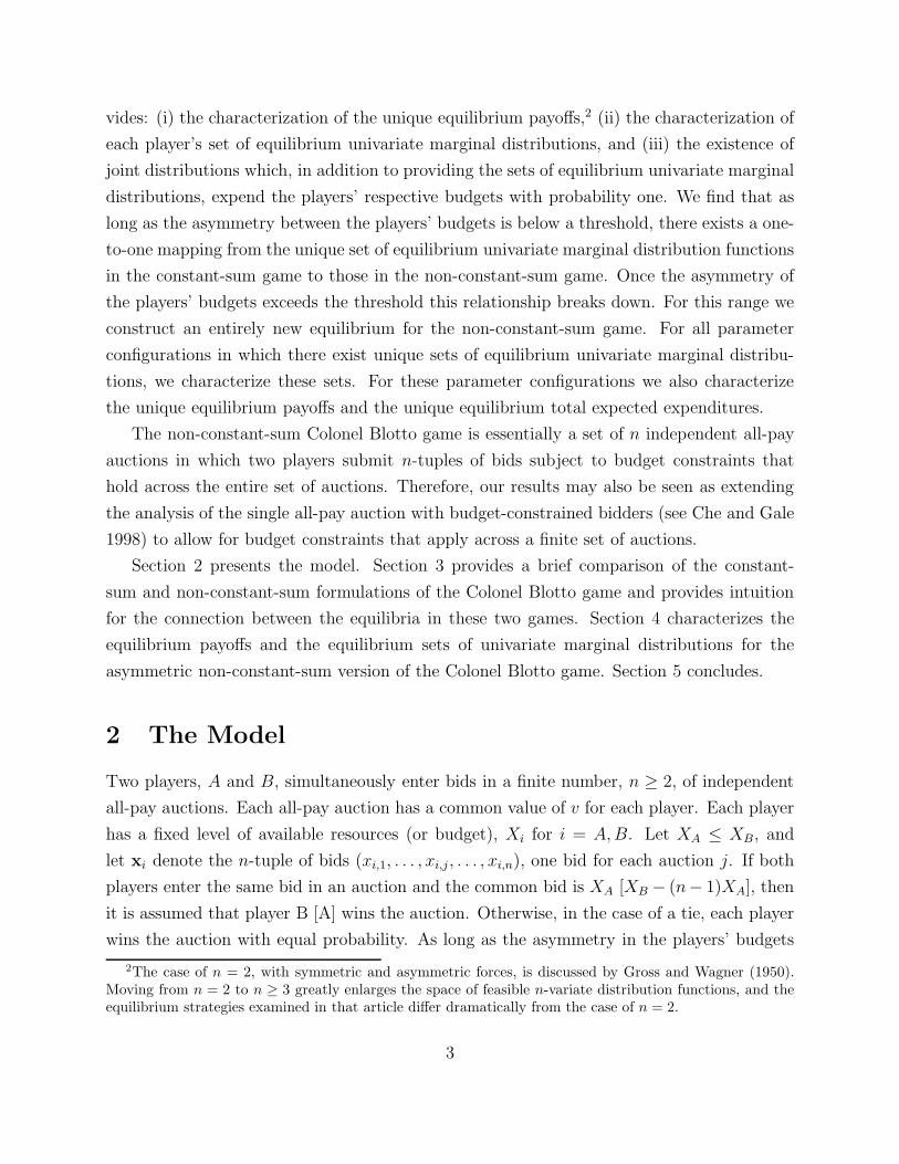
vides: (i) the characterization of the unique equilibrium payoffs,2 (ii) the characterization of

each player’s set of equilibrium univariate marginal distributions, and (iii) the existence of

joint distributions which, in addition to providing the sets of equilibrium univariate marginal

distributions, expend the players’ respective budgets with probability one. We find that as

long as the asymmetry between the players’ budgets is below a threshold, there exists a one-

to-one mapping from the unique set of equilibrium univariate marginal distribution functions

in the constant-sum game to those in the non-constant-sum game. Once the asymmetry of

the players’ budgets exceeds the threshold this relationship breaks down. For this range we

construct an entirely new equilibrium for the non-constant-sum game. For all parameter

configurations in which there exist unique sets of equilibrium univariate marginal distribu-

tions, we characterize these sets. For these parameter configurations we also characterize

the unique equilibrium payoffs and the unique equilibrium total expected expenditures.

The non-constant-sum Colonel Blotto game is essentially a set of n independent all-pay

auctions in which two players submit n-tuples of bids subject to budget constraints that

hold across the entire set of auctions. Therefore, our results may also be seen as extending

the analysis of the single all-pay auction with budget-constrained bidders (see Che and Gale

1998) to allow for budget constraints that apply across a finite set of auctions.

Section 2 presents the model. Section 3 provides a brief comparison of the constant-

sum and non-constant-sum formulations of the Colonel Blotto game and provides intuition

for the connection between the equilibria in these two games. Section 4 characterizes the

equilibrium payoffs and the equilibrium sets of univariate marginal distributions for the

asymmetric non-constant-sum version of the Colonel Blotto game. Section 5 concludes.

2 The Model

Two players, A and B, simultaneously enter bids in a finite number, n ≥ 2, of independent

all-pay auctions. Each all-pay auction has a common value of v for each player. Each player

has a fixed level of available resources (or budget), Xi for i = A,B. Let XA ≤ XB, and

let xi denote the n-tuple of bids (xi,1, . . . , xi,j , . . . , xi,n), one bid for each auction j. If both

players enter the same bid in an auction and the common bid is XA [XB − (n− 1)XA], then

it is assumed that player B [A] wins the auction. Otherwise, in the case of a tie, each player

wins the auction with equal probability. As long as the asymmetry in the players’ budgets

2The case of n = 2, with symmetric and asymmetric forces, is discussed by Gross and Wagner (1950).Moving from n = 2 to n ≥ 3 greatly enlarges the space of feasible n-variate distribution functions, and theequilibrium strategies examined in that article differ dramatically from the case of n = 2.

3

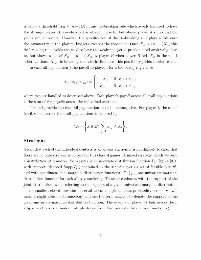
is below a threshold [XB ≤ (n− 1)XA], any tie-breaking rule which avoids the need to have

the stronger player B provide a bid arbitrarily close to, but above, player A’s maximal bid

yields similar results. However, the specification of the tie-breaking rule plays a role once

the asymmetry in the players’ budgets exceeds the threshold. Once XB > (n − 1)XA, this

tie-breaking rule avoids the need to have the weaker player A provide a bid arbitrarily close

to, but above, a bid of XB − (n − 1)XA by player B when player B bids XA in the n − 1

other auctions. Any tie-breaking rule which eliminates this possibility yields similar results.

In each all-pay auction j the payoff to player i for a bid of xi,j is given by

πi,j (xi,j, x−i,j) =

v − xi,j if xi,j > x−i,j

−xi,j if xi,j < x−i,j

where ties are handled as described above. Each player’s payoff across all n all-pay auctions

is the sum of the payoffs across the individual auctions.

The bid provided to each all-pay auction must be nonnegative. For player i, the set of

feasible bids across the n all-pay auctions is denoted by

Bi =

{x ∈ R

n+

∣∣∣∣n∑

j=1

xi,j ≤ Xi

}.

Strategies

Given that each of the individual contests is an all-pay auction, it is not difficult to show that

there are no pure strategy equilibria for this class of games. A mixed strategy, which we term

a distribution of resources, for player i is an n-variate distribution function Pi : Rn+ → [0, 1]

with support (denoted Supp(Pi)) contained in the set of player i’s set of feasible bids Bi

and with one-dimensional marginal distribution functions {Fi,j}nj=1, one univariate marginal

distribution function for each all-pay auction j. To avoid confusion with the support of the

joint distribution, when referring to the support of a given univariate marginal distribution

— the smallest closed univariate interval whose complement has probability zero — we will

make a slight abuse of terminology and use the term domain to denote the support of the

given univariate marginal distribution function. The n-tuple of player i’s bids across the n

all-pay auctions is a random n-tuple drawn from the n-variate distribution function Pi.

4

The Non-Constant-Sum Colonel Blotto game

The N-C-S Colonel Blotto game, which we label

NCB{XA, XB, n, v

},

is the one-shot game in which players compete by simultaneously announcing distributions

of resources subject to their budget constraints, each all-pay auction is won by the player

that provides the higher bid in that auction (where in the case of a tie the tie-breaking rule

described above applies), and players’ receive the sum of their payoffs across the individual

all-pay auctions.

3 Relationship Between the Two Formulations

Before proceeding with the equilibrium analysis, it is instructive to provide intuition for the

connection between the equilibria in the constant-sum and non-constant-sum formulations of

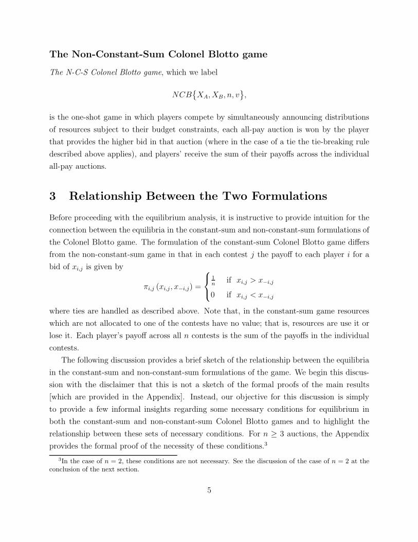
the Colonel Blotto game. The formulation of the constant-sum Colonel Blotto game differs

from the non-constant-sum game in that in each contest j the payoff to each player i for a

bid of xi,j is given by

πi,j (xi,j , x−i,j) =

1n

if xi,j > x−i,j

0 if xi,j < x−i,j

where ties are handled as described above. Note that, in the constant-sum game resources

which are not allocated to one of the contests have no value; that is, resources are use it or

lose it. Each player’s payoff across all n contests is the sum of the payoffs in the individual

contests.

The following discussion provides a brief sketch of the relationship between the equilibria

in the constant-sum and non-constant-sum formulations of the game. We begin this discus-

sion with the disclaimer that this is not a sketch of the formal proofs of the main results

[which are provided in the Appendix]. Instead, our objective for this discussion is simply

to provide a few informal insights regarding some necessary conditions for equilibrium in

both the constant-sum and non-constant-sum Colonel Blotto games and to highlight the

relationship between these sets of necessary conditions. For n ≥ 3 auctions, the Appendix

provides the formal proof of the necessity of these conditions.3

3In the case of n = 2, these conditions are not necessary. See the discussion of the case of n = 2 at theconclusion of the next section.

5

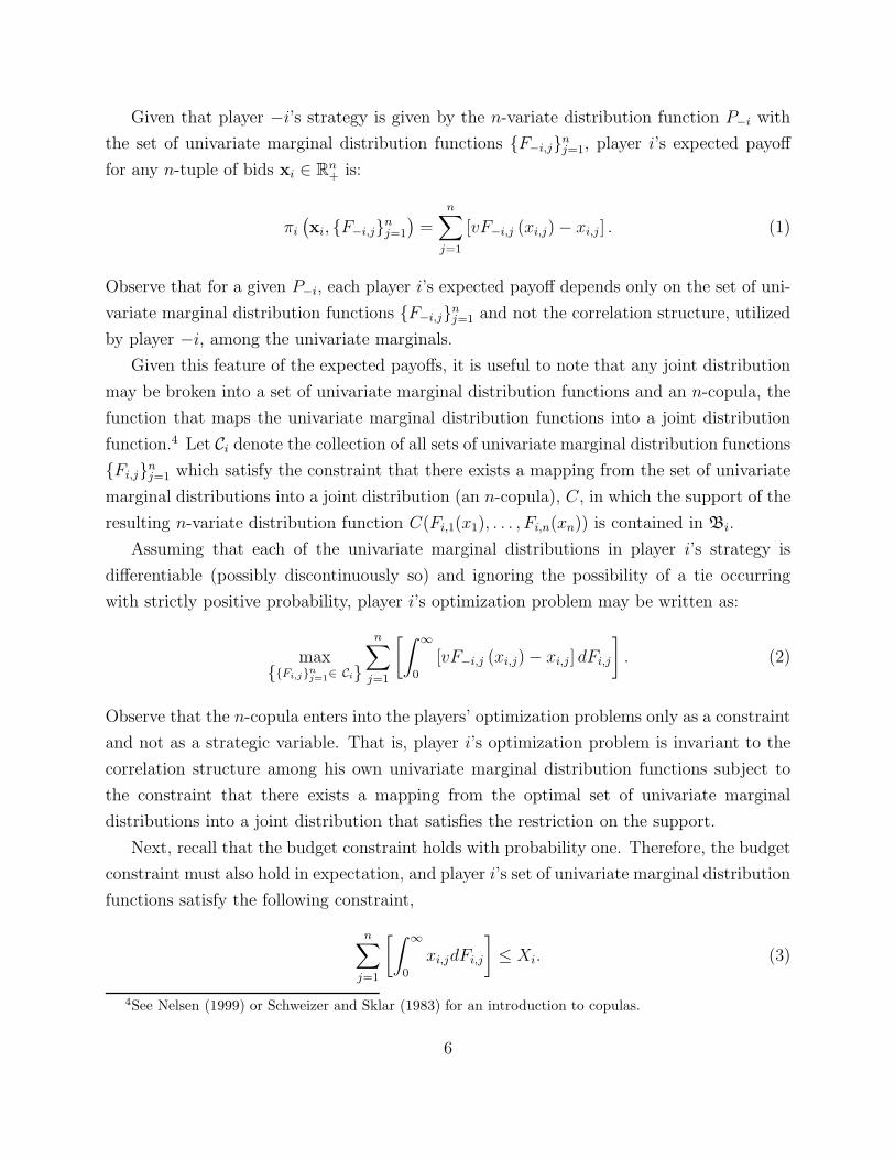
Given that player −i’s strategy is given by the n-variate distribution function P−i with

the set of univariate marginal distribution functions {F−i,j}nj=1, player i’s expected payoff

for any n-tuple of bids xi ∈ Rn+ is:

πi

(xi, {F−i,j}

nj=1

)=

n∑

j=1

[vF−i,j (xi,j)− xi,j ] . (1)

Observe that for a given P−i, each player i’s expected payoff depends only on the set of uni-

variate marginal distribution functions {F−i,j}nj=1 and not the correlation structure, utilized

by player −i, among the univariate marginals.

Given this feature of the expected payoffs, it is useful to note that any joint distribution

may be broken into a set of univariate marginal distribution functions and an n-copula, the

function that maps the univariate marginal distribution functions into a joint distribution

function.4 Let Ci denote the collection of all sets of univariate marginal distribution functions

{Fi,j}nj=1 which satisfy the constraint that there exists a mapping from the set of univariate

marginal distributions into a joint distribution (an n-copula), C, in which the support of the

resulting n-variate distribution function C(Fi,1(x1), . . . , Fi,n(xn)) is contained in Bi.

Assuming that each of the univariate marginal distributions in player i’s strategy is

differentiable (possibly discontinuously so) and ignoring the possibility of a tie occurring

with strictly positive probability, player i’s optimization problem may be written as:

max{{Fi,j}nj=1∈ Ci}

n∑

j=1

[∫ ∞

0

[vF−i,j (xi,j)− xi,j ] dFi,j

]. (2)

Observe that the n-copula enters into the players’ optimization problems only as a constraint

and not as a strategic variable. That is, player i’s optimization problem is invariant to the

correlation structure among his own univariate marginal distribution functions subject to

the constraint that there exists a mapping from the optimal set of univariate marginal

distributions into a joint distribution that satisfies the restriction on the support.

Next, recall that the budget constraint holds with probability one. Therefore, the budget

constraint must also hold in expectation, and player i’s set of univariate marginal distribution

functions satisfy the following constraint,

n∑

j=1

[∫ ∞

0

xi,jdFi,j

]≤ Xi. (3)

4See Nelsen (1999) or Schweizer and Sklar (1983) for an introduction to copulas.

6

Given that equation (3) is a constraint on only the set of univariate marginal distributions

functions, it will be useful to include this constraint in player i’s optimization problem. Thus,

we have that player i’s optimization problem from equation (2) may now be written as,

max{{Fi,j}nj=1∈ Ci}

n∑

j=1

[∫ ∞

0

[vF−i,j (xi,j)− (1 + λi)xi,j ] dFi,j

]+ λiXi. (4)

This optimization problem is essentially a variational problem involving the maximization

of a collection of functionals with the side constraints that there exist a sufficient n-copula

and that each univariate marginal distribution is a weakly increasing function. The n Euler-

Lagrange equations provide a set of necessary conditions for equilibrium. For each j =

1, . . . , n the corresponding Euler-Lagrange equation is given by

d

dx[vF−i,j (xi,j)− (1 + λi) xi,j] = 0. (5)

Rearranging terms slightly, it becomes clear that for each auction j equation (5) is precisely

the necessary condition that holds for one isolated all-pay auction without a budget con-

straint and in which the prize has value v/(1+λi), henceforth the implicit value of the prize.

The intuition is that the constraint on the total expenditure across all auctions implicitly

imposes an opportunity cost λi ≥ 0 of resource expenditure.5 Therefore, the cost of allocat-

ing xj resources to auction j entails not only the explicit cost of the bid but also the implicit

opportunity cost from not being able to use those resources in another auction. An increase

in the implicit opportunity cost of a bid has the dual interpretation of lowering the implicit

value of the prize.

Applying a similar line of reasoning to the constant-sum Colonel Blotto game, it is

straightforward to derive the set of necessary conditions for equilibrium given by the n Euler-

Lagrange equations for that optimization problem. For each j = 1, . . . , n the corresponding

Euler-Lagrange equation is given by

d

dx

[1

nF−i,j (xi,j)− λixi,j

]= 0. (6)

In this case we see that for each contest j equation (6) is precisely the necessary condition

that holds for one isolated all-pay auction without a budget constraint and in which the

5Note that λi takes the value of zero in the event that player i does not benefit from the relaxation of hisbudget constraint.

7

prize has value 1/(nλi).

As long as there exists a sufficient n-copula, each of the unique equilibrium univariate

marginal distribution functions in the two games corresponds directly to the unique equi-

librium univariate distribution function in a single two-player all-pay auction with complete

information and with each player i’s values for the prizes given by v/(1 + λi) and 1/(nλi)

respectively [see Hillman and Riley 1989; Baye, Kovenock, and de Vries 1996]. Therefore,

there exists a one-to-one mapping from the unique set of equilibrium univariate marginal

distributions in the non-constant-sum game to those in the constant-sum game as long as

there exists a sufficient n-copula.

Generically speaking, the constraint on the n-copula is non-binding if for each player the

intersection of the hyperplane formed by the n-tuples which exhaust his respective budget

and the n-box formed by the domains of each of the univariate marginal distributions for the

corresponding all-pay auctions is well behaved. For example consider the case in which the

n-box formed by the domains is [0, XA]n. If XB > (n−1)XA, then it is clear that there exist

no n-tuples in the intersection of the hyperplane {x ∈ Rn+

∣∣∑nj=1 xj = XB} and the n-box

[0, XA]n in which any xj = 0. Thus, the support of player B’s distribution of resources cannot

be completely contained in his budget-balancing hyperplane and have univariate marginals

with domain [0, XA].

In the constant-sum game, the constraint on the existence of a sufficient n-copula is non-

binding as long as (2/n) < (XA/XB) ≤ 1. Within this region, which is illustrated in Panel

(i) of Figure 1, Theorem 2 of Roberson (2006) characterizes the unique sets of equilibrium

univariate marginal distribution functions and Theorem 4 of that article provides the proof

of the existence of a sufficient n-copula for this range.

[Insert Figure 1 here]

Before tracing out the corresponding region for the non-constant-sum formulation of

the game, observe that Panel (i) of Figure 1 also delineates the regions of the parameter

space that correspond to Theorems 3 and 5 of Roberson (2006), labelled regions 3 and 5

respectively. In these regions, in which (1/n) < (XA/XB) ≤ (2/n), there exists a correspond-

ing parameter region in the non-constant-sum game over which the equilibrium univariate

marginal distribution functions in the two games are related. However, this relationship

is not necessarily one-one. The issue is that the constraint on the existence of a sufficient

8

n-copula comes into play and the sets of univariate marginal distributions must be adjusted

accordingly. In the two games these adjustments may vary.

For the constant-sum game’s remaining parameter configuration XA ≤ (XB/n) the play-

ers are at the extreme end of the asymmetry spectrum. Over this parameter region, the

stronger player (B) has a sufficient level of resources to win each of the n contests with

certainty, and, due to the use it or lose it feature of the constant-sum formulation, that

game becomes trivial. In this region there is no relationship between the two games. Due

to the relaxation of the use it or lose it feature, the non-constant-sum game is never trivial,

and in this range we construct entirely new equilibrium distributions of resources for the

non-constant-sum game.

We now introduce what we term themodified budgets for the non-constant-sum game with

n ≥ 3. In the expressions for the modified budgets we define the sets Tk for k = 1, 2, 3, 5

to denote the portion of the parameter space that is covered by the corresponding theorem

number k(= 1, 2, 3, 5) in the following section.6 These regions are delineated as follows.

T1:{(XA, XB) ∈ R

2+

∣∣( 2n)min{v,XB} < XA ≤ XB

}

T2:{(XA, XB) ∈ R

2+

∣∣XB/(n − 1) ≤ XA ≤ ( 2n)min{v,XB} or XA = 2v

nand XB >

v(2− 2n)}

T3:{(XA, XB) ∈ R

2+

∣∣XA < (2vn) and XA ≤ max

{XB− 2v

n

n−2, XB

n

}}

T5:{(XA, XB) ∈ R

2+

∣∣max{

XB− 2vn

n−2, XB

n

}< XA < XB

n−1

}

Recall that the floor function ⌊x⌋ denotes the largest integer less than or equal to x. Player

A’s modified budget is given by

MXA(XA, XB) =

min{XA,

nv2

}if (XA,XB) ∈ T1

XA if (XA,XB) ∈ T2

n(XA)2

2v if (XA,XB) ∈ T3

XA −(1−

nXA2v

)(nXA−XB)

⌊XA

XB−(n−1)XA⌋+1

if (XA,XB) ∈ T5

6Theorem 4 is a proof of the existence of a pair of n-variate joint distributions which satisfy the conditionsspecified in Theorem 3.

9

and player B’s modified budget is given by

MXB(XA, XB) =

min{XB,

nv2 ,(nvXA

2

)1/2}if (XA, XB) ∈ T1

min{XB, v

(2− 2

n

)}if (XA, XB) ∈ T2

n(XA −

X2A

2v

)if (XA, XB) ∈ T3

nXA(nXB−(n−1)2XA)2v +

(1− n(XB−(n−2)XA)

2v

)(⌊

XA

XB−(n−1)XA

⌋

+2)

XA

⌊

XA

XB−(n−1)XA

⌋

+1if (XA, XB) ∈ T5

It will be useful to define the set of n-tuples which exhaust the modified budgets MXAand

MXB. Let Bi denote this set, defined as

Bi =

{x ∈ R

n+

∣∣∣∣n∑

j=1

xi,j = MXi(XA, XB)

},

and note that Bi ⊂ Bi.

The players’ modified budgets, which are illustrated in (XA, XB)-space as the shaded re-

gions in Panel (ii) of Figure 1, are the equilibrium total expected expenditures for each of the

equilibria examined in the following section [i.e., for player i,MXi=∑

j EFi,j(xi,j)]. As shown

in the Appendix [see Lemma 2], in the T1 and T2 parameter regions with XA 6= (2v/n),

these equilibrium total expected expenditures are unique. In the remaining parameter re-

gions, there exist other payoff non-equivalent equilibria.

Note that given a pair of resource levels XA and XB which satisfy (XA, XB) ∈ T1

there are three possible cases: (a) neither player uses all of their available resources [i.e.,

MXA= nv/2 and MXB

= nv/2], (b) only (the weaker) player A uses all of his available

resources [i.e., MXA= XA and MXB

= (nvXA/2)1/2], and (c) both players A and B use all

of their available resources [i.e., MXA= XA and MXB

= XB]. The regions corresponding to

each of these cases appears in Panel (ii) of Figure 1 as 1a, 1b, and 1c respectively. Given

that in the constant-sum game resources are use it or lose it, such considerations do not arise

in that game.

It is important to observe that when XA and XB satisfy the condition that XA ∈

((2/n)min{v,XB}, XB] [i.e., regions 1a, 1b, and 1c of Panel (ii) of Figure 1], the modi-

fied budgets satisfy the corresponding condition that (2/n) < (MXA/MXB

) ≤ 1. As we will

show, there exists a one-to-one correspondence between the sets of equilibrium univariate

marginal distribution functions that arise in this region and those that arise in the constant-

sum game for the region (2/n) < (XA/XB) ≤ 1. This characterization is formally stated in

Theorem 1 of the next section.

Similarly, for XA and XB which lie in regions 2 and 5 [which correspond to Theo-

10

rems 2 and 5] of Panel (ii) of Figure 1, the modified budgets satisfy the condition that

(1/n) < (MXA/MXB

) ≤ (2/n). In these regions the sets of equilibrium univariate marginal

distribution functions are related to those arising in the constant-sum game for the param-

eter range (1/n) < (XA/XB) ≤ (2/n). But as mentioned before, this relationship is not

necessarily one-one.

For all budget configurations (XA, XB) which lie in region 3 of panel (ii), we construct

an entirely new set of equilibrium distributions of resources [see Theorem 3]. Note that

this region covers not only the portion of the parameter space which corresponds to the

trivial region of the constant-sum game [i.e., XA ≤ (XB/n)], but also a portion of the

parameter space in which the constant-sum game is non-trivial. Again, this breakdown in

the relationship between the equilibria in the two games occurs in sufficiently asymmetric

regions of the parameter space because of the discrepancy in the value of unused resources

in the two formulations.

To summarize, whereas there is a one-to-one relationship between the unique equilibrium

sets of univariate marginal distribution functions in the constant-sum and and non-constant-

sum versions of the game — when the asymmetry between the players’ budgets is below a

threshold — this relationship is non-linear with respect to the players’ budgets but is linear

with respect to the players’ modified budgets.

4 Equilibrium Distributions of Resources

The following Theorems examine the equilibrium distributions of resources for all parameter

configurations of the non-constant-sum Colonel Blotto game with n ≥ 3 auctions. This

section concludes with the case of n = 2 auctions. In the Theorem 1 parameter range we

characterize each player’s unique set of equilibrium univariate marginal distributions. In the

Theorem 2 parameter range with XA 6= (2v/n) we characterize the unique set of equilibrium

univariate marginal distributions for player A and provide an equilibrium distribution of

resources for player B. Over this range player B does not have a unique set of equilibrium

univariate marginal distribution functions.7 In the Theorem 3 and 5 parameter ranges we

provide an equilibrium distribution of resources for each player. Over this range neither

player has a unique set of univariate marginal distribution functions.8 For the Theorem

7An alternative set of equilibrium univariate marginal distribution functions is provided in the discussionfollowing Lemma 7 in the Appendix.

8For information on the non-uniqueness of the univariate marginals over the Theorem 5 [3] parameterrange, see the discussion preceding Theorem 5 [at the conclusion of the Appendix].

11

1 and 2 parameter ranges with XA 6= (2v/n) the equilibrium expected payoffs and the

equilibrium total expected expenditures are unique [see Lemma 2 in the the Appendix].

Three or more Auctions

For the game NCB{XA, XB, n, v} with n ≥ 3, Theorem 1 examines all parameter configu-

rations which lie in the 1a, 1b, and 1c regions of panel (ii) of Figure 1. Recall that in these

regions the resulting modified budgets satisfy the condition (2/n) < (MXA/MXB

) ≤ 1.

Theorem 1. Let XA, XB, v, and n ≥ 3 satisfy (2/n)min{v,XB} < XA ≤ XB (equivalently

(2/n) < (MXA/MXB

) ≤ 1). The pair of n-variate distribution functions P ∗A and P ∗

B constitute

a Nash equilibrium of the game NCB{XA, XB, n, v} if and only if they satisfy the following

two conditions: (1) For each player i, Supp(P ∗i ) ⊂ Bi and (2) P ∗

i , i = A,B, provides

the corresponding unique set of univariate marginal distribution functions {F ∗i,j}

nj=1 outlined

below.

∀ j ∈ {1, . . . , n} F ∗A,j (xj) =

(1−

MXA

MXB

)+

xj

(2/n)MXB

(MXA

MXB

)for xj ∈

[0, 2

nMXB

].

∀ j ∈ {1, . . . , n} F ∗B,j (xj) =

xj

(2/n)MXB

for xj ∈[0, 2

nMXB

].

The unique equilibrium expected payoff for player A is (nvMXA/2MXB

) − MXA, and the

unique equilibrium expected payoff for player B is nv (1− (MXA/2MXB

))−MXB. The unique

equilibrium total expected expenditure for player A is MXA(XA, XB) = min{XA, (nv/2)},

and the unique equilibrium total expected expenditure for player B is MXB(XA, XB) =

min{XB, (nv/2), (nvXA/2)1/2}.

The existence of a pair of n-variate distribution functions which satisfy conditions (1)

and (2) of Theorem 1 is provided in Roberson (2006). In particular, Theorem 4 of Roberson

(2006) establishes the existence of n-variate distribution functions for which Supp(P ∗i ) ⊂ Bi

and that provide the necessary sets of univariate marginal distribution functions given in

Theorem 1. The proof of the uniqueness of the equilibrium sets of univariate marginal

distribution functions, equilibrium payoffs, and equilibrium total expected expenditures is

given in the Appendix.

Although it is straightforward to show that any pair of n-variate distribution functions

which satisfy conditions (1) and (2) of Theorem 1 form an equilibrium, it is useful to provide

the intuition for this result. We begin with the expected payoffs for each player. Let P ∗B

denote a feasible n-variate distribution function for player B with the univariate marginal

12

distributions {F ∗B,j}

nj=1 given in Theorem 1. If player B is using P ∗

B, then player A’s expected

payoff πA, when player A chooses any n-tuple of bids xA ∈ BA

⋂[0, (2/n)MXB

]n [i.e., one

bid for each of the n all-pay auctions such that∑

j xA,j ≤ XA and xA,j ∈ [0, (2/n)MXB] for

each auction j], is

πA (xA, P∗B) =

n∑

j=1

[vF ∗

B,j (xA,j)− xA,j

].

Recall that for all j, F ∗B,j (xj) =

xj

(2/n)MXB

for xj ∈ [0, (2/n)MXB]. Simplifying yields

πA (xA, P∗B) =

(nv

2MXB

− 1

) n∑

j=1

xA,j . (7)

Similarly, the expected payoff πB to player B from any n-tuple of bids xB ∈ BB

⋂(0, (2/n)MXB

]n

— when player A uses a feasible n-variate distribution P ∗A with the univariate marginal dis-

tributions {F ∗A,j}

nj=1 given in Theorem 1 — follows directly,

πB (xB, P∗A) = nv

(1−

MXA

MXB

)+

(nvMXA

2M2XB

− 1

) n∑

j=1

xB,j . (8)

Observe that neither player can bid below 0 and that bidding above (2/n)MXBis suboptimal.

Thus, for the Theorem 1 parameter range equations (7) and (8) provide the maximal payoffs

(for player A and player B respectively) for any feasible n-tuple of bids across the n all-pay

auctions.

Recall that there are three possible cases: (a) neither player uses all of his available

resources, (b) only (the weaker) player A uses all of his available resources, and (c) both

players A and B use all of their available resources. These three regions are shown graphically

in panel (ii) of Figure 1 as regions 1a, 1b, and 1c respectively. Suppose that we are in case

(a) in which neither player uses all of his available resources. Case (a) corresponds to

the situation in which the total value of the n auctions nv is low enough relative to the

players’ budgets that neither player has incentive to commit all of his resources. In the

Theorem 1 parameter range player A’s modified budget is given by MXA= min{XA, nv/2}.

If player A does not use all of his budget, then it must be that XA > (nv/2) and so

MXA= (nv/2). Similarly from player B’s modified budget in the Theorem 1 range [MXB

=

min{XB, nv/2, (nvXA/2)1/2}], it follows that if player A (the weaker player) is not using all

of his budget then MXB= (nv/2). Because MXA

= MXB= (nv/2), the expected payoffs

given in (7) and (8) are πA (xA, P∗B) = 0 and πB (xB, P

∗A) = 0 respectively. Observe that

13

in case (a) neither player has incentive to change their total resource expenditure,∑

j xi,j ,

across the n all-pay auctions. That is, because MXA= MXB

= (nv/2) and the opponent is

using the equilibrium strategy, the expected payoff to player i, given in equations (7) and

(8), is zero for all xi ∈ [0, v]n regardless of player i’s total expenditure,∑

j xi,j , in the n

all-pay auctions.

Now suppose that we are in case (b) in which only player A uses all of his budget. Case

(b) corresponds to the situation in which the total value of the n all-pay auctions nv is high

enough that the weaker player optimally commits all of his resources but not so high that

the stronger player must also commit all of his resources to the n all-pay auctions. From

the preceding discussion it follows that XA ≤ (nv/2) and thus MXA= XA. If player B is

not using all of his budget then from MXB= min{XB, nv/2, (nvXA/2)

1/2}, it must be that

XB > (nvXA/2)1/2 and so MXB

= (nvXA/2)1/2. Inserting MXA

and MXBinto equations (7)

and (8) and simplifying yields

πA (xA, P∗B) =

((nv

2XA

)1/2

− 1

)n∑

j=1

xA,j (9)

and

πB (xB, P∗A) = nv

(1−

(2XA

nv

)1/2). (10)

Recall that in case (b) XA ≤ (nv/2) and so ((nv/2XA)1/2−1) ≥ 0. From equation (9) we see

that player A is indifferent with regards to which all-pay auctions to commit resources to,

but has incentive to increase his total resource expenditure across the n all-pay auctions [i.e.,∑

j xA,j ]. However in case (b), player A’s equilibrium distribution of resources P ∗A expends

his budget with probability one [i.e., at each point bA ∈ Supp(P ∗A),

∑j xA,j = XA].

9 From

equation (10) we see that, when MXA= XA and MXB

= (nvXA/2)1/2 are inserted into

player B’s expected payoff given in equation (8), player B’s expected payoff is the same for

all n-tuples xB ∈ (0, (2nvXA)1/2]n. That is player B’s expected payoff is independent of his

total expenditure∑

j xB,j [so long as xB ∈ (0, 2(nvXA/2)1/2]n], and so player B does not

have incentive to change his total resource expenditure across the n all-pay auctions.

Finally, suppose that we are in case (c) in which each player is at his respective budget

constraint. Case (c) corresponds to the situation in which the total value of the n all-pay

9Recall that Roberson (2006) establishes the existence of n-variate distribution functions for whichSupp(P ∗

i ) ⊂ Bi, and that in this case MXA= XA. It follows directly that player A expends his bud-

get with probability one.

14

auctions nv is high enough that both players optimally commit all of their resources to the

n all-pay auctions. Thus, MXA= XA and MXB

= XB. From equations (7) and (8) it follows

that

πA (xA, P∗B) =

(nv

2XB− 1

) n∑

j=1

xA,j (11)

and

πB (xB, P∗A) = nv

(1−

XA

XB

)+

(nvXA

2X2B

− 1

) n∑

j=1

xB,j . (12)

In case (c), XA < (nv/2) and XB < (nvXA/2)1/2 < (nv/2). Observe in equation (11)

that ((nv/2XB) − 1) > 0 and, thus, player A has incentive to increase his total resource

expenditure across the n all-pay auctions, but in his equilibrium distribution of resources P ∗A

he is already at his budget constraint with probability one [i.e., at each point xA ∈ Supp(P ∗A),∑

j xA,j = XA]. Similarly, in equation (12) ((nvXA/2X2B)− 1) > 0 and, thus, player B has

incentive to increase his total resource expenditure across the n all-pay auctions, but in

his equilibrium distribution of resources P ∗B he is already at his budget constraint with

probability one [i.e., at each point xB ∈ Supp(P ∗B),

∑j xB,j = XB].

Because Roberson (2006) demonstrates the existence of a pair of n-variate distributions

{P ∗A,, P

∗A,} in which Supp(P ∗

i ) ⊂ Bi for i = A,B and that provides the sets of univariate

marginal distributions specified in condition (2) of Theorem 1, it follows from the arguments

given above that such a pair of n-variate distribution functions constitute an equilibrium

in all three cases (a), (b), and (c). The proof of the uniqueness of the sets of univariate

marginal distributions is given in the Appendix.

Once (MXA/MXB

) = (2/n) both the uniqueness of player B’s set of equilibrium univariate

marginal distributions and the relationship with the two-player all-pay auction with complete

information fail to hold. The reason for this breakdown is that once XB/(n − 1) ≤ XA ≤

(2/n)min{v,XB}, or equivalently(1/(n−1)) ≤ (MXA/MXB

) ≤ (2/n), it is possible for player

B’s set of equilibrium univariate marginals to have atoms that lie strictly within the interior

and at the upper bound of the domain and player B’s equilibrium total expected expenditure

is not unique.10 In Theorem 2 we provide the unique set of equilibrium univariate marginal

distributions for player A and provide an equilibrium set of univariate marginal distributions

for player B.

Theorem 2. Let XA, XB, v, and n ≥ 3 satisfy XB/(n − 1) ≤ XA ≤ (2/n)min{v,XB} or

XA = (2v/n) and XB > v(2 − (2/n)) [equivalently 1/(n− 1) ≤ (MXA/MXB

) ≤ (2/n)]. The

10See the discussion at the conclusion of the Appendix.

15

n-variate distribution function P ∗A is a Nash equilibrium strategy for player A in the game

NCB{XA, XB, n, v} if and only if it satisfies the following two conditions: (1) Supp(P ∗A) ⊂

BA and (2) P ∗A provides the corresponding set of univariate marginal distribution functions

{F ∗A,j}

nj=1 outlined below.

∀ j ∈ {1, . . . , n} F ∗A,j (xj) =

(1− 2

n

)+

xj

XA

(2n

)for xj ∈ [0, XA] .

Sufficient conditions for P ∗B to be a Nash equilibrium strategy include: Supp(P ∗

B) ⊂ BB

and that P ∗B provides the corresponding set of univariate marginal distribution functions

{F ∗B,j}

nj=1 outlined below.

∀ j ∈ {1, . . . , n} F ∗B,j (xj) =

2xj

(XA−

MXBn

)

(XA)2for xj ∈ [0, XA)

1 for xj ≥ XA

.

In equilibria satisfying these conditions on P ∗A and P ∗

B, the expected payoff for player A is

2v(1−(MXB/nXA))−XA, the expected payoff for player B is nv−2v(1−(MXB

/nXA))−MXB,

the total expected expenditure for player A is MXA(XA, XB) = XA, and the total expected

expenditure for player B is MXB(XA, XB) = min{XB, v(2− (2/n))}.

If XA 6= (2v/n), then the equilibrium expected payoffs and total expected expenditures are

unique. In the event that XA = (2v/n) player B’s equilibrium total expected expenditure is

not unique. As a direct consequence player A’s equilibrium expected payoff is not unique

when XA = (2v/n).

The existence of a pair of n-variate distribution functions which satisfy Theorem 2’s

necessary and sufficient condition for player A and sufficient condition for player B is pro-

vided in Theorem 4 of Roberson (2006). For XA 6= (2v/n), the proof of uniqueness for

the equilibrium payoffs, the equilibrium total expected expenditures, and player A’s set of

univariate marginal distributions is given in the Appendix. If XA = (2v/n), then there exist

equilibria in which player B uses strategies PB in which∑

j EFB,j(xB,j) 6= MXB

(XA, XB),

where for (XA, XB) ∈ T2, MXB(XA, XB) = min{XB, v(2 − (2/n))}. In fact, there exist a

continuum of equilibria in which PB satisfies a modified form of the sufficient conditions

given in Theorem 2. The modification to the sufficient conditions for P ∗B is that the term

MXBin the univariate marginal distributions given above may be replaced by any value in

the set [v,min{XB, v(2− (2/n))}]. In this case it is clear that the equilibrium payoffs are not

unique. Player B’s set of equilibrium univariate marginal distributions is, also, not unique,

16

and an alternative set of equilibrium univariate marginal distributions for player B is given

in the discussion at the conclusion of the Appendix.

To sketch the proof that a pair of n-variate distributions that satisfy the conditions of

Theorem 2 form an equilibrium, let P ∗B denote a feasible n-variate distribution for player

B with the univariate marginal distributions {F ∗B,j}

nj=1 given in Theorem 2. If player B is

using P ∗B, then player A’s expected payoff πA, when player A chooses any n-tuple of bids

xA ∈ BA

⋂[0, XA]

n, is

πA (xA, P∗B) =

(2v (XA − (MXB

/n))

X2A

− 1

) n∑

j=1

xA,j. (13)

Note that (2v/X2A)(XA − (MXB

/n))− 1 ≥ 0 is equivalent to MXB≤ (n− (nXA/2v))XA. If

XA < (2v/n), it follows from equation (13) that player A has incentive to choose n-tuples

xA ∈ [0, XA]n such that

∑j xA,j = XA. When XA = (2v/n), player A’s expected payoff from

any n-tuple xA ∈ [0, XA]n is zero.

Similarly, the expected payoff πB to player B from any n-tuple of bids across the n all-pay

auctions xB ∈ BB

⋂(0, XA]

n, when player A uses a feasible n-variate distribution P ∗A with

the univariate marginal distributions {F ∗A,j}

nj=1 given in Theroem 2, is

πB (xB, P∗A) = nv

(1−

2

n

)+

(2v

nXA

− 1

) n∑

j=1

xB,j . (14)

Because XA ≤ (2v/n) it follows that (2v/nXA) − 1 ≥ 0. If XA < (2v/n), player B has

incentive to choose n-tuples xB ∈ (0, XA]n such that

∑j xB,j = XB. If XA = (2v/n), then

any n-tuple xB ∈ (0, XA]n provides player B with an expected payoff of nv(1− (2/n)).

Seeing that Roberson (2006) demonstrates the existence of a pair of n-variate distribu-

tions that result in the sets of univariate marginal distributions given in Theorem 2 and

that satisfy the respective budget restrictions with probability one [i.e., for i = A,B at each

point bi ∈ Supp(P ∗i ),∑

j xi,j = MXi], it follows from the arguments given above that such a

pair of n-variate distribution functions constitute an equilibrium. The proof of uniqueness

of player A’s set of univariate marginal distributions is given in the Appendix.

The following Theorem constructs entirely new equilibrium distributions of resources for

the highly asymmetric portion of the parameter space in which the relationship between the

constant-sum and non-constant-sum versions of the game breaks down.

Theorem 3. Let XA, XB, v, and n ≥ 3 satisfy XA < (2v/n) and XA ≤ max{(XB −

17

2vn)/(n−2), XB/n}. The pair of n-variate distribution functions P ∗

A and P ∗B constitute a Nash

equilibrium of the game NCB{XA, XB, n, v} if they satisfy the following two conditions: (1)

For each player i, Supp(P ∗i ) ⊂ Bi and (2) P ∗

i , i = A,B, provides the corresponding set of

univariate marginal distribution functions {F ∗i,j}

nj=1 outlined below.

∀ j ∈ {1, . . . , n} FA,j (xj) =(1− XA

v

)+

xj

vfor xj ∈ [0, XA] .

∀ j ∈ {1, . . . , n} FB,j (xj) =

xj

vfor xj ∈ [0, XA)

1 for xj ≥ XA

.

In equilibria satisfying these conditions on P ∗A and P ∗

B, the expected payoff for player A is 0,

the expected payoff for player B is nv(1− (XA/v)), the total expected expenditure for player

A is (XA)2(n/2v), and the total expected expenditure for player B is n(XA − (XA)

2/2v).

We begin with a sketch of the proof that a pair of n-variate distribution functions which

satisfy the conditions of Theorem 3 form an equilibrium, and then move on to the proof of

existence of such a pair of n-variate distribution functions.

To see that these two sets of univariate marginal distributions form an equilibrium in

the Theorem 3 parameter region, let P ∗B denote a feasible n-variate distribution for player

B with the univariate marginal distributions {F ∗B,j}

nj=1 given in Theorem 3. If player B is

using P ∗B, then player A’s expected payoff πA, when player A chooses any n-tuple of bids

xA ∈ BA is

πA (xA, P∗B) = 0. (15)

From equation (15), player A does not have incentive to increase or decrease his total ex-

penditure in the n all-pay auctions.

Similarly, the expected payoff πB to player B from any n-tuple of bids across the n all-pay

auctions xB ∈ BB

⋂(0, XA]

n, when player A uses a feasible n-variate distribution P ∗A with

the univariate marginal distributions {F ∗A,j}

nj=1 given in Theorem 3, is

πB (xB, P∗A) = nv

(1−

XA

v

). (16)

Thus, player B also has the same expected payoff for each xB ∈ (0, XA]n and therefore has

no incentive to increase or decrease his total expenditure in the n all-pay auctions.

Assuming that there exists a pair of n-variate distribution functions which satisfy condi-

tions (1) and (2) of Theorem 3, it follows from the arguments given above that such a pair

18

of n-variate distribution functions constitute an equilibrium. We now establish the existence

of sufficient n-variate distributions for the Theorem 3 parameter range.

Theorem 4. For each set of equilibrium univariate marginal distribution functions, {Fi,j}nj=1,

given in Theorem 3, there exists an n-copula, C, such that the support of the n-variate dis-

tribution function C(Fi,1(x1), . . . , Fi,n(xn)) is contained in Bi.

We begin with the proof for player A. The construction of a sufficient n-variate distribu-

tion function for player A and XA ≥ (v/n) is outlined as follows [recall that in the Theorem

3 parameter region XA < (2v/n)]. The remaining case that XA < (v/n) is addressed directly

following this case.

1. Player A selects n− 2 of the all-pay auctions, each all-pay auction chosen with equal

probability, and bids zero in each of those all-pay auctions.

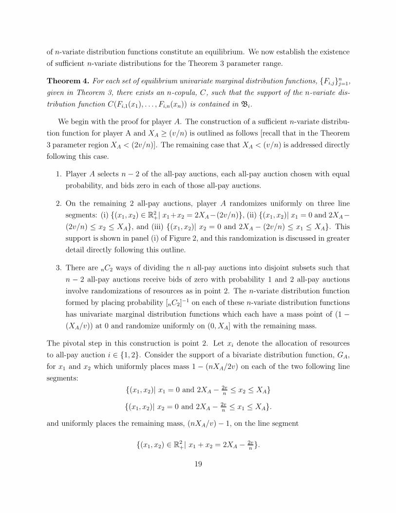
2. On the remaining 2 all-pay auctions, player A randomizes uniformly on three line

segments: (i) {(x1, x2) ∈ R2+| x1+x2 = 2XA−(2v/n)}, (ii) {(x1, x2)| x1 = 0 and 2XA−

(2v/n) ≤ x2 ≤ XA}, and (iii) {(x1, x2)| x2 = 0 and 2XA − (2v/n) ≤ x1 ≤ XA}. This

support is shown in panel (i) of Figure 2, and this randomization is discussed in greater

detail directly following this outline.

3. There are nC2 ways of dividing the n all-pay auctions into disjoint subsets such that

n − 2 all-pay auctions receive bids of zero with probability 1 and 2 all-pay auctions

involve randomizations of resources as in point 2. The n-variate distribution function

formed by placing probability [nC2]−1 on each of these n-variate distribution functions

has univariate marginal distribution functions which each have a mass point of (1 −

(XA/v)) at 0 and randomize uniformly on (0, XA] with the remaining mass.

The pivotal step in this construction is point 2. Let xi denote the allocation of resources

to all-pay auction i ∈ {1, 2}. Consider the support of a bivariate distribution function, GA,

for x1 and x2 which uniformly places mass 1 − (nXA/2v) on each of the two following line

segments:

{(x1, x2)| x1 = 0 and 2XA − 2vn≤ x2 ≤ XA}

{(x1, x2)| x2 = 0 and 2XA − 2vn≤ x1 ≤ XA}.

and uniformly places the remaining mass, (nXA/v)− 1, on the line segment

{(x1, x2) ∈ R2+| x1 + x2 = 2XA − 2v

n}.

19

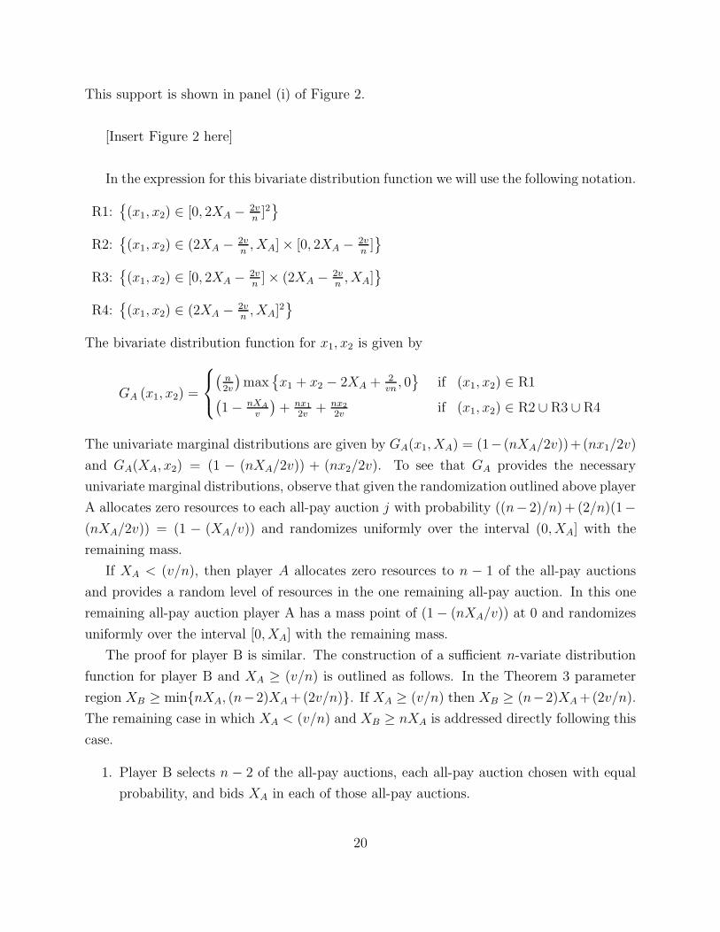
This support is shown in panel (i) of Figure 2.

[Insert Figure 2 here]

In the expression for this bivariate distribution function we will use the following notation.

R1:{(x1, x2) ∈ [0, 2XA − 2v

n]2}

R2:{(x1, x2) ∈ (2XA − 2v

n, XA]× [0, 2XA − 2v

n]}

R3:{(x1, x2) ∈ [0, 2XA − 2v

n]× (2XA − 2v

n, XA]

}

R4:{(x1, x2) ∈ (2XA − 2v

n, XA]

2}

The bivariate distribution function for x1, x2 is given by

GA (x1, x2) =

(n2v

)max

{x1 + x2 − 2XA + 2

vn, 0}

if (x1, x2) ∈ R1(1− nXA

v

)+ nx1

2v+ nx2

2vif (x1, x2) ∈ R2 ∪ R3 ∪ R4

The univariate marginal distributions are given by GA(x1, XA) = (1− (nXA/2v))+(nx1/2v)

and GA(XA, x2) = (1 − (nXA/2v)) + (nx2/2v). To see that GA provides the necessary

univariate marginal distributions, observe that given the randomization outlined above player

A allocates zero resources to each all-pay auction j with probability ((n− 2)/n)+ (2/n)(1−

(nXA/2v)) = (1 − (XA/v)) and randomizes uniformly over the interval (0, XA] with the

remaining mass.

If XA < (v/n), then player A allocates zero resources to n − 1 of the all-pay auctions

and provides a random level of resources in the one remaining all-pay auction. In this one

remaining all-pay auction player A has a mass point of (1− (nXA/v)) at 0 and randomizes

uniformly over the interval [0, XA] with the remaining mass.

The proof for player B is similar. The construction of a sufficient n-variate distribution

function for player B and XA ≥ (v/n) is outlined as follows. In the Theorem 3 parameter

region XB ≥ min{nXA, (n−2)XA+(2v/n)}. If XA ≥ (v/n) then XB ≥ (n−2)XA+(2v/n).

The remaining case in which XA < (v/n) and XB ≥ nXA is addressed directly following this

case.

1. Player B selects n − 2 of the all-pay auctions, each all-pay auction chosen with equal

probability, and bids XA in each of those all-pay auctions.

20

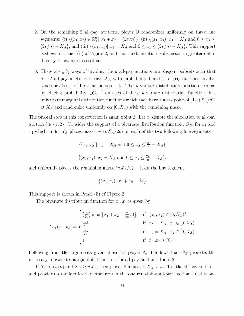
2. On the remaining 2 all-pay auctions, player B randomizes uniformly on three line

segments: (i) {(x1, x2) ∈ R2+| x1 + x2 = (2v/n)}, (ii) {(x1, x2)| x1 = XA and 0 ≤ x2 ≤

(2v/n)−XA}, and (iii) {(x1, x2)| x2 = XA and 0 ≤ x1 ≤ (2v/n)−XA}. This support

is shown in Panel (ii) of Figure 2, and this randomization is discussed in greater detail

directly following this outline.

3. There are nC2 ways of dividing the n all-pay auctions into disjoint subsets such that

n − 2 all-pay auctions receive XA with probability 1 and 2 all-pay auctions involve

randomizations of force as in point 2. The n-variate distribution function formed

by placing probability [nC2]−1 on each of these n-variate distribution functions has

univariate marginal distribution functions which each have a mass point of (1−(XA/v))

at XA and randomize uniformly on [0, XA) with the remaining mass.

The pivotal step in this construction is again point 2. Let xi denote the allocation to all-pay

auction i ∈ {1, 2}. Consider the support of a bivariate distribution function, GB, for x1 and

x2 which uniformly places mass 1− (nXA/2v) on each of the two following line segments

{(x1, x2)| x1 = XA and 0 ≤ x2 ≤2vn−XA}

{(x1, x2)| x2 = XA and 0 ≤ x1 ≤2vn−XA}.

and uniformly places the remaining mass, (nXA/v)− 1, on the line segment

{(x1, x2)| x1 + x2 =2vn}

This support is shown in Panel (ii) of Figure 2.

The bivariate distribution function for x1, x2 is given by

GB (x1, x2) =

(n2v

)max

{x1 + x2 −

2vn, 0}

if (x1, x2) ∈ [0, XA)2

nx1

2vif x2 = XA, x1 ∈ [0, XA)

nx2

2vif x1 = XA, x2 ∈ [0, XA)

1 if x1, x2 ≥ XA

Following from the arguments given above for player A, it follows that GB provides the

necessary univariate marginal distributions for all-pay auctions 1 and 2.

If XA < (v/n) and XB ≥ nXA, then player B allocates XA to n−1 of the all-pay auctions

and provides a random level of resources in the one remaining all-pay auction. In this one

21

remaining all-pay auction player B has a mass point of (1− (nXA/v)) at XA and randomizes

uniformly over the interval [0, XA) with the remaining mass.

This completes the proof of the existence of sufficient n-variate distributions for the

Theorem 3 parameter range.

In the remaining region in which max{(XB − 2vn)/(n−2), XB/n} < XA < XB/(n−1), as

in the corresponding constant-sum parameter range, both players have atoms in the interior

of the domains of their univariate marginal distribution functions. It should be noted that

in this region the results are sensitive to the specification of the tie-breaking rule.

Let ∆ denote the amount of resources available to player B if player B has bid XA in

n− 1 of the auctions:

∆ = XB − (n− 1)XA.

Recalling that the floor function ⌊x⌋ denotes the largest integer less than or equal to x, define

k as

k =⌊ XA

XB − (n− 1)XA

⌋=⌊XA

∆

⌋.

In this region of the parameter space, (n− 1)XA < XB < nXA and so k ≥ 1. It will also be

helpful to note that XA/(k + 1) < ∆ ≤ XA/k.

In this region of the parameter space the sets of equilibrium univariate marginal distri-

butions are not unique.

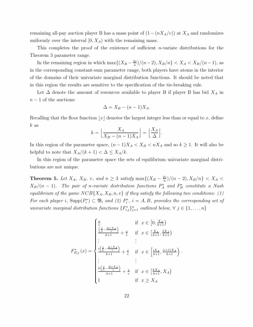
Theorem 5. Let XA, XB, v, and n ≥ 3 satisfy max{(XB − 2vn)/(n − 2), XB/n} < XA <

XB/(n − 1). The pair of n-variate distribution functions P ∗A and P ∗

B constitute a Nash

equilibrium of the game NCB{XA, XB, n, v} if they satisfy the following two conditions: (1)

For each player i, Supp(P ∗i ) ⊂ Bi and (2) P ∗

i , i = A,B, provides the corresponding set of

univariate marginal distribution functions {F ∗i,j}

nj=1 outlined below, ∀ j ∈ {1, . . . , n}

F ∗B,j (x) =

xv

if x ∈[0, XA

k+1

)(

2n−

∆+XAv

)

k+1+ x

vif x ∈

[XA

k+1, 2XA

k+1

)

......

i(

2n−

∆+XAv

)

k+1+ x

vif x ∈

[iXA

k+1, (i+1)XA

k+1

)

......

k(

2n−

∆+XAv

)

k+1+ x

vif x ∈

[kXA

k+1, XA

)

1 if x ≥ XA

.

22

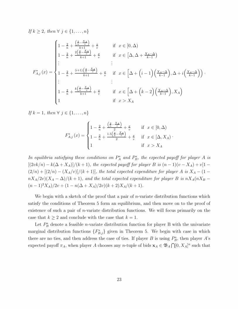
If k ≥ 2, then ∀ j ∈ {1, . . . , n}

F ∗A,j (x) =

1− 2n+

(2n−

XAv

)

k+1+ x

vif x ∈ [0,∆)

1− 2n+

2(

2n−

XAv

)

k+1+ x

vif x ∈

[∆,∆+ XA−∆

k−1

)

......

1− 2n+

(i+1)(

2n−

XAv

)

k+1+ x

vif x ∈

[∆+

(i− 1

)(XA−∆k−1

),∆+ i

(XA−∆k−1

))

......

1− 2n+

k(

2n−

XAv

)

k+1+ x

vif x ∈

[∆+

(k − 2

)(XA−∆k−1

), XA

)

1 if x > XA

.

If k = 1, then ∀ j ∈ {1, . . . , n}

F ∗A,j (x) =

1− 2n+

(2n−

XAv

)

2+ x

vif x ∈ [0,∆)

1− 2n+

1.5(

2n−

XAv

)

2+ x

vif x ∈ [∆, XA)

1 if x > XA

.

In equilibria satisfying these conditions on P ∗A and P ∗

B, the expected payoff for player A is

[(2vk/n)− k(∆ +XA)]/(k + 1), the expected payoff for player B is (n− 1)(v −XA) + v[1−

(2/n) + [(2/n)− (XA/v)]/(k + 1)], the total expected expenditure for player A is XA − (1 −

nXA/2v)(XA −∆)/(k + 1), and the total expected expenditure for player B is nXA(nXB −

(n− 1)2XA)/2v + (1− n(∆ +XA)/2v)(k + 2)XA/(k + 1).

We begin with a sketch of the proof that a pair of n-variate distribution functions which

satisfy the conditions of Theorem 5 form an equilibrium, and then move on to the proof of

existence of such a pair of n-variate distribution functions. We will focus primarily on the

case that k ≥ 2 and conclude with the case that k = 1.

Let P ∗B denote a feasible n-variate distribution function for player B with the univariate

marginal distribution functions {F ∗B,j} given in Theorem 5. We begin with case in which

there are no ties, and then address the case of ties. If player B is using P ∗B, then player A’s

expected payoff πA, when player A chooses any n-tuple of bids xA ∈ BA

⋂[0, XA]

n such that

23

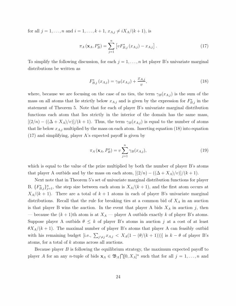
for all j = 1, . . . , n and i = 1, . . . , k + 1, xA,j 6= iXA/(k + 1), is

πA (xA, P∗B) =

n∑

j=1

[vF ∗

B,j (xA,j)− xA,j

]. (17)

To simplify the following discussion, for each j = 1, . . . , n let player B’s univariate marginal

distributions be written as

F ∗B,j (xA,j) = γB(xA,j) +

xA,j

v, (18)

where, because we are focusing on the case of no ties, the term γB(xA,j) is the sum of the

mass on all atoms that lie strictly below xA,j and is given by the expression for F ∗B,j in the

statement of Theorem 5. Note that for each of player B’s univariate marginal distribution

functions each atom that lies strictly in the interior of the domain has the same mass,

[(2/n) − ((∆ + XA)/v)]/(k + 1). Thus, the term γB(xA,j) is equal to the number of atoms

that lie below xA,j multiplied by the mass on each atom. Inserting equation (18) into equation

(17) and simplifying, player A’s expected payoff is given by

πA (xA, P∗B) = v

n∑

j=1

γB(xA,j), (19)

which is equal to the value of the prize multiplied by both the number of player B’s atoms

that player A outbids and by the mass on each atom, [(2/n)− ((∆ +XA)/v)]/(k + 1).

Next note that in Theorem 5’s set of univariate marginal distribution functions for player

B, {F ∗B,j}

nj=1, the step size between each atom is XA/(k + 1), and the first atom occurs at

XA/(k + 1). There are a total of k + 1 atoms in each of player B’s univariate marginal

distributions. Recall that the rule for breaking ties at a common bid of XA in an auction

is that player B wins the auction. In the event that player A bids XA in auction j, then

— because the (k + 1)th atom is at XA — player A outbids exactly k of player B’s atoms.

Suppose player A outbids θ ≤ k of player B’s atoms in auction j at a cost of at least

θXA/(k + 1). The maximal number of player B’s atoms that player A can feasibly outbid

with his remaining budget [i.e.,∑

j′ 6=j xA,j < XA(1 − (θ/(k + 1)))] is k − θ of player B’s

atoms, for a total of k atoms across all auctions.

Because player B is following the equilibrium strategy, the maximum expected payoff to

player A for an any n-tuple of bids xA ∈ BA

⋂[0, XA]

n such that for all j = 1, . . . , n and

24

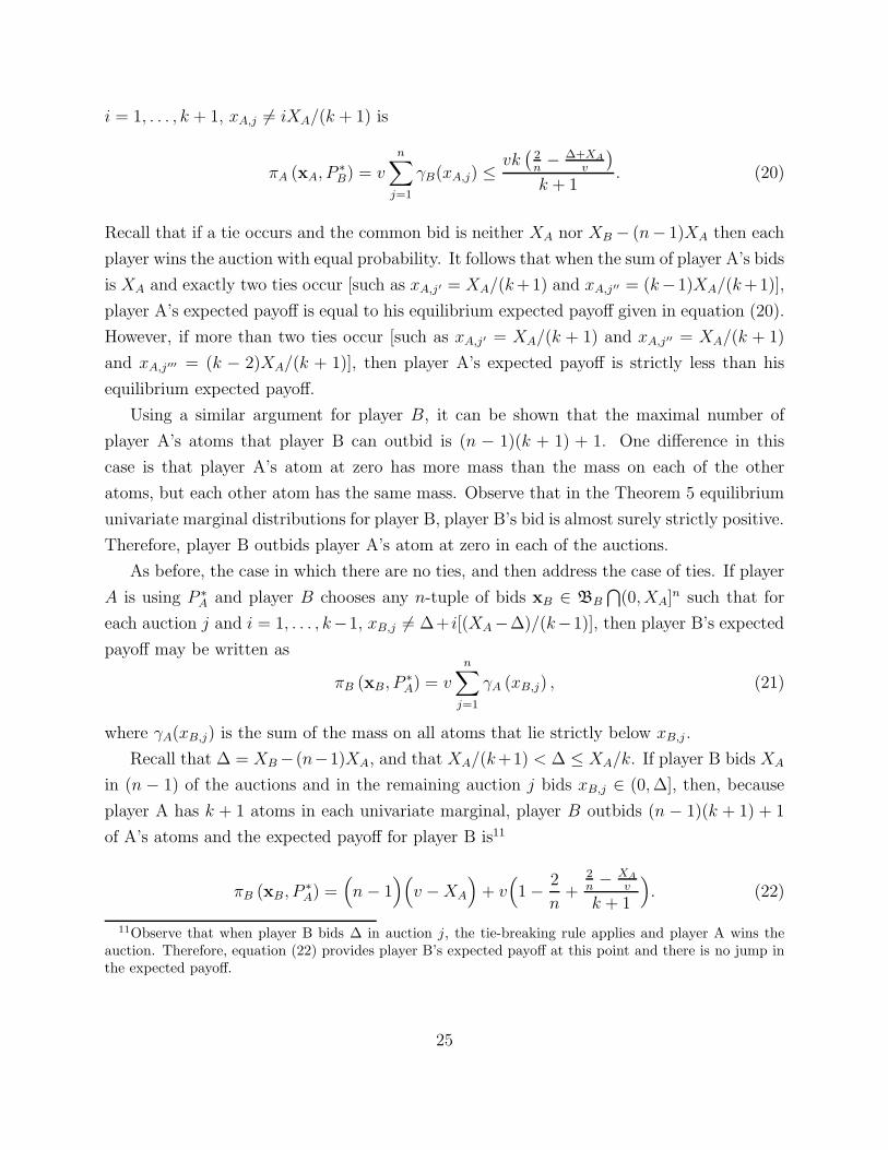
i = 1, . . . , k + 1, xA,j 6= iXA/(k + 1) is

πA (xA, P∗B) = v

n∑

j=1

γB(xA,j) ≤vk(2n− ∆+XA

v

)

k + 1. (20)

Recall that if a tie occurs and the common bid is neither XA nor XB − (n− 1)XA then each

player wins the auction with equal probability. It follows that when the sum of player A’s bids

is XA and exactly two ties occur [such as xA,j′ = XA/(k+1) and xA,j′′ = (k−1)XA/(k+1)],

player A’s expected payoff is equal to his equilibrium expected payoff given in equation (20).

However, if more than two ties occur [such as xA,j′ = XA/(k + 1) and xA,j′′ = XA/(k + 1)

and xA,j′′′ = (k − 2)XA/(k + 1)], then player A’s expected payoff is strictly less than his

equilibrium expected payoff.

Using a similar argument for player B, it can be shown that the maximal number of

player A’s atoms that player B can outbid is (n − 1)(k + 1) + 1. One difference in this

case is that player A’s atom at zero has more mass than the mass on each of the other

atoms, but each other atom has the same mass. Observe that in the Theorem 5 equilibrium

univariate marginal distributions for player B, player B’s bid is almost surely strictly positive.

Therefore, player B outbids player A’s atom at zero in each of the auctions.

As before, the case in which there are no ties, and then address the case of ties. If player

A is using P ∗A and player B chooses any n-tuple of bids xB ∈ BB

⋂(0, XA]

n such that for

each auction j and i = 1, . . . , k−1, xB,j 6= ∆+ i[(XA−∆)/(k−1)], then player B’s expected

payoff may be written as

πB (xB, P∗A) = v

n∑

j=1

γA (xB,j) , (21)

where γA(xB,j) is the sum of the mass on all atoms that lie strictly below xB,j .

Recall that ∆ = XB− (n−1)XA, and that XA/(k+1) < ∆ ≤ XA/k. If player B bids XA

in (n − 1) of the auctions and in the remaining auction j bids xB,j ∈ (0,∆], then, because

player A has k + 1 atoms in each univariate marginal, player B outbids (n − 1)(k + 1) + 1

of A’s atoms and the expected payoff for player B is11

πB (xB, P∗A) =

(n− 1

)(v −XA

)+ v(1−

2

n+

2n− XA

v

k + 1

). (22)

11Observe that when player B bids ∆ in auction j, the tie-breaking rule applies and player A wins theauction. Therefore, equation (22) provides player B’s expected payoff at this point and there is no jump inthe expected payoff.

25

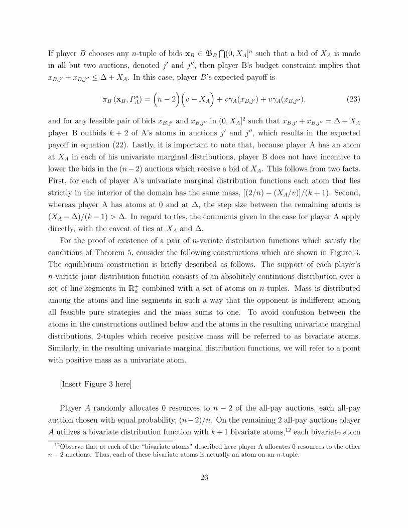
If player B chooses any n-tuple of bids xB ∈ BB

⋂(0, XA]

n such that a bid of XA is made

in all but two auctions, denoted j′ and j′′, then player B’s budget constraint implies that

xB,j′ + xB,j′′ ≤ ∆+XA. In this case, player B’s expected payoff is

πB (xB, P∗A) =

(n− 2

)(v −XA

)+ vγA(xB,j′) + vγA(xB,j′′), (23)

and for any feasible pair of bids xB,j′ and xB,j′′ in (0, XA]2 such that xB,j′ + xB,j′′ = ∆+XA

player B outbids k + 2 of A’s atoms in auctions j′ and j′′, which results in the expected

payoff in equation (22). Lastly, it is important to note that, because player A has an atom

at XA in each of his univariate marginal distributions, player B does not have incentive to

lower the bids in the (n−2) auctions which receive a bid of XA. This follows from two facts.

First, for each of player A’s univariate marginal distribution functions each atom that lies

strictly in the interior of the domain has the same mass, [(2/n)− (XA/v)]/(k + 1). Second,

whereas player A has atoms at 0 and at ∆, the step size between the remaining atoms is

(XA −∆)/(k− 1) > ∆. In regard to ties, the comments given in the case for player A apply

directly, with the caveat of ties at XA and ∆.

For the proof of existence of a pair of n-variate distribution functions which satisfy the

conditions of Theorem 5, consider the following constructions which are shown in Figure 3.

The equilibrium construction is briefly described as follows. The support of each player’s

n-variate joint distribution function consists of an absolutely continuous distribution over a

set of line segments in R+n combined with a set of atoms on n-tuples. Mass is distributed

among the atoms and line segments in such a way that the opponent is indifferent among

all feasible pure strategies and the mass sums to one. To avoid confusion between the

atoms in the constructions outlined below and the atoms in the resulting univariate marginal

distributions, 2-tuples which receive positive mass will be referred to as bivariate atoms.

Similarly, in the resulting univariate marginal distribution functions, we will refer to a point

with positive mass as a univariate atom.

[Insert Figure 3 here]

Player A randomly allocates 0 resources to n − 2 of the all-pay auctions, each all-pay

auction chosen with equal probability, (n−2)/n. On the remaining 2 all-pay auctions player

A utilizes a bivariate distribution function with k+1 bivariate atoms,12 each bivariate atom

12Observe that at each of the “bivariate atoms” described here player A allocates 0 resources to the othern− 2 auctions. Thus, each of these bivariate atoms is actually an atom on an n-tuple.

26

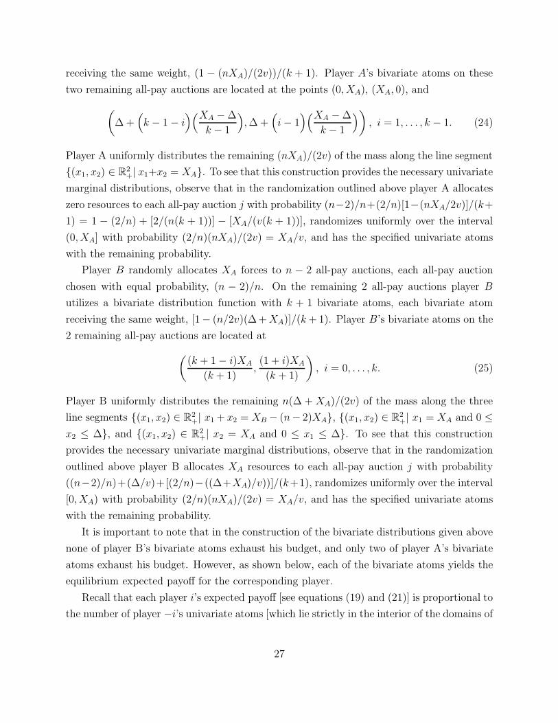
receiving the same weight, (1 − (nXA)/(2v))/(k + 1). Player A’s bivariate atoms on these

two remaining all-pay auctions are located at the points (0, XA), (XA, 0), and

(∆+

(k − 1− i

)(XA −∆

k − 1

),∆+

(i− 1

)(XA −∆

k − 1

)), i = 1, . . . , k − 1. (24)

Player A uniformly distributes the remaining (nXA)/(2v) of the mass along the line segment

{(x1, x2) ∈ R2+| x1+x2 = XA}. To see that this construction provides the necessary univariate

marginal distributions, observe that in the randomization outlined above player A allocates

zero resources to each all-pay auction j with probability (n−2)/n+(2/n)[1−(nXA/2v)]/(k+

1) = 1 − (2/n) + [2/(n(k + 1))] − [XA/(v(k + 1))], randomizes uniformly over the interval

(0, XA] with probability (2/n)(nXA)/(2v) = XA/v, and has the specified univariate atoms

with the remaining probability.

Player B randomly allocates XA forces to n − 2 all-pay auctions, each all-pay auction

chosen with equal probability, (n − 2)/n. On the remaining 2 all-pay auctions player B

utilizes a bivariate distribution function with k + 1 bivariate atoms, each bivariate atom

receiving the same weight, [1− (n/2v)(∆+XA)]/(k+1). Player B’s bivariate atoms on the

2 remaining all-pay auctions are located at

((k + 1− i)XA

(k + 1),(1 + i)XA

(k + 1)

), i = 0, . . . , k. (25)

Player B uniformly distributes the remaining n(∆ + XA)/(2v) of the mass along the three

line segments {(x1, x2) ∈ R2+| x1 + x2 = XB − (n− 2)XA}, {(x1, x2) ∈ R

2+| x1 = XA and 0 ≤

x2 ≤ ∆}, and {(x1, x2) ∈ R2+| x2 = XA and 0 ≤ x1 ≤ ∆}. To see that this construction

provides the necessary univariate marginal distributions, observe that in the randomization

outlined above player B allocates XA resources to each all-pay auction j with probability

((n−2)/n)+(∆/v)+[(2/n)−((∆+XA)/v))]/(k+1), randomizes uniformly over the interval

[0, XA) with probability (2/n)(nXA)/(2v) = XA/v, and has the specified univariate atoms

with the remaining probability.

It is important to note that in the construction of the bivariate distributions given above

none of player B’s bivariate atoms exhaust his budget, and only two of player A’s bivariate

atoms exhaust his budget. However, as shown below, each of the bivariate atoms yields the

equilibrium expected payoff for the corresponding player.

Recall that each player i’s expected payoff [see equations (19) and (21)] is proportional to

the number of player −i’s univariate atoms [which lie strictly in the interior of the domains of

27

player −i’s univariate marginal distributions] which are outbid. As can be seen in Figure 3,

for each player i each of his bivariate atoms outbids the same number of player −i’s univariate

atoms as in his equilibrium expected payoff [k atoms for player A and (n− 2)(k+1)+ k+2

for player B].13 It is straightforward, albeit tedious, to show this algebraically. The key step

in this is given by the following inequality

(k − i)XA

k + 1< ∆+

(k − 1− i

)(XA −∆

k − 1

)<

(k + 1− i)XA

k + 1, (26)

which holds for all i = 1, . . . , k − 1. This inequality follows directly from the relationship

between ∆, k, and XA. In particular, XA/(k + 1) < ∆ ≤ XA/k.

The inequality in equation (26) shows that when player A bids ∆ + (k − 1 − i)((XA −

∆)/(k − 1)) in an auction she outbids k − i of player B’s univariate atoms in that auction.

Conversely, as equation (26) holds for all i = 1, . . . , k − 1, it also shows that when player

B bids (k + 1 − i)XA/(k + 1) in an auction she outbids k + 1 − i of player A’s univariate

atoms in that auction. From the locations of each player’s bivariate atoms given in equations

(24) and (25), it follows that for each player i each of his bivariate atoms outbids the same

number of player −i’s univariate atoms as in his equilibrium expected payoff [k atoms for

player A and (n− 2)(k+1)+ k+2 for player B]. This completes the proof of Theorem 5 for

k ≥ 2.

We now address the case of k = 1. Just as with k ≥ 2, the sets of equilibrium univariate

marginal distributions are not unique, but, as shown in Lemma 3 of the Appendix, the

equilibrium expected payoffs are unique. For k = 1 the construction specified above for

player A fails to be feasible given his budget constraint. In this case, player A’s univariate

marginals are modified, but for player B the construction specified above, but with k = 1,

still applies.

The sketch of the proof that a pair of n-variate distribution functions, which satisfy the

conditions of Theorem 5 with k = 1, form an equilibrium follows along the same lines as for

k ≥ 2. For the proof of existence of such an n-variate distribution function for player A,

consider the following construction.

Player A randomly allocates 0 resources to n − 2 of the all-pay auctions, each all-

pay auction chosen with equal probability, (n − 2)/n. On the remaining 2 all-pay auc-

13Consider for example, player A’s bivariate atom at the point (0, XA). This is the left most atom inpanel (i) of Figure 3. When player A chooses this bivariate atom, he outbids (due to the tie-breaking rule)all but one (k = 3) of player B’s (univariate) atoms in the x2 direction and none of player B’s univariateatoms in the x1 direction. Similarly, at each of his bivariate atoms player A outbids a total of k of playerA’s univariate atoms. The case for player B follows directly.

28

tions player A utilizes a bivariate distribution function with 4 bivariate atoms, each bi-

variate atom receiving the same weight, (1 − (nXA)/(2v))/4. Player A’s bivariate atoms

on these two remaining all-pay auctions are located at the points (0, XA), (XA, 0), (0,∆),

and (∆, 0). Player A uniformly distributes the remaining (nXA)/(2v) of the mass along

the line segment {(x1, x2) ∈ R2+| x1 + x2 = XA}. To see that this construction pro-

vides the necessary univariate marginal distributions, observe that in the randomization

outlined above player A allocates zero resources to each all-pay auction j with probability

(n− 2)/n+ (2/n)[1− (nXA/2v)]/2 = 1− (2/n) + (1/n)− [XA/(2v)], randomizes uniformly

over the interval (0, XA] with probability (2/n)(nXA)/(2v) = XA/v, and has the specified

univariate atoms with the remaining probability.

As before, two of player A’s atoms do not exhaust player A’s budget. However, each of

these bivariate atoms clearly outbids one of player B’s univariate atoms and results in the

unique equilibrium expected payoff for player A.

Two Auctions

Before outlining the case of two auctions, it is important to note that for n = 2 the sets

of equilibrium univariate marginal distributions are non-unique for all parameter regions.14

However, as is shown in the Appendix, in the Theorem 1 and 2 parameter ranges with

XA 6= (2v/n) the equilibrium payoffs and total expenditures are unique.

Recall that in both panels of Figure 1, the parameter space is partitioned by the four

rays: (a) XA = XB/n, (b) XA = XB/(n − 1), (c) XA = 2XB/n, and (d) XA = XB. In

the case that n = 2, the last three of these collapse to the single ray XA = XB, and the

first of these becomes XA = XB/2. The following partition of the parameter space, for

n = 2, provides the portions of the parameter space in which the theorems in the preceding

subsection provide sufficient, but not necessary, conditions for equilibrium.

T1*:{(XA, XB) ∈ R

2+

∣∣v < XA ≤ XB

}

T2*:{(XA, XB) ∈ R

2+

∣∣XB = XA ≤ v or XA = v and XB > v}

T3a*:{(XA, XB) ∈ R

2+

∣∣XB ≥ v and XB

2< XA < v

}

T3b*:{(XA, XB) ∈ R

2+

∣∣XA < v and XA ≤ XB

2

}

14With n = 2 each player’s pair of univariate marginals need not be independent of the identity of theauction. For example, the location of and/or the mass placed on atoms need not be symmetric acrossauctions. For further information see Macdonell and Mastronardi (2010).

29

T5*:{(XA, XB) ∈ R

2+

∣∣XB < v and XB

2< XA < v

}

These regions and the resulting modified budgets are illustrated in Figure 4 below.

[Insert Figure 4 here]

Recall that in the constructions provided for the Theorem 3 and 5 parameter regions,

each player allocated a specified bid to (n− 2) of the all-pay auctions [for player A this was

a bid of 0, and for player B this was a bid of XA]. When n = 2, (n − 2)/n = 0 and the

constructions for both of those regions simply become the bivariate distributions that were

specified for the remaining two auctions. It is straightforward to show that in the Theorem

1 and 2 regions the Frechet-Hoeffding lower bound 2-copula combined with the univariate

marginals specified in Theorems 1 and 2, which for player i = A,B are given by

P ∗i (bi,1, bi,2) = max

{F ∗i,1 (bi,1) + F ∗

i,2 (bi,2)− 1, 0},

results in a pair of bivariate distribution functions for which Supp(P ∗i ) ⊂ Bi and that provide

an equilibrium pair of univariate marginal distribution functions.

5 Conclusion

Kvasov (2007) introduces a non-constant-sum version of the Colonel Blotto game which

relaxes the “use it or lose it” feature of the traditional constant-sum formulation of the

game. In the case of symmetric budgets, that article establishes that there exists a one-to-one

mapping from the set of unique univariate marginal distribution functions in the constant-

sum game to those in the non-constant-sum game. As the analysis of the non-constant-sum

version of the Colonel Blotto game is extended to allow for asymmetric budget constraints,

we find that — as long as the level of asymmetry between the players’ budgets is below

a threshold — there still exists a one-to-one mapping from the unique set of equilibrium

univariate marginal distribution functions in the constant-sum game to those in the non-

constant-sum game. The classic Colonel Blotto game provides an important benchmark in

the study of the logic of strategic multi-dimensional conflict, and, as our results show, the

nature of the incentives in such conflicts remain largely unchanged when the use it or lose it

feature of the constant-sum game is relaxed.

30

Appendix

For the Theorem 1 parameter range with n ≥ 3 (denoted as T1), this Appendix charac-

terizes each player’s unique: set of equilibrium univariate marginal distribution functions,

equilibrium payoffs, and equilibrium total expected expenditures. We also show that the

uniqueness of the equilibrium payoffs and equilibrium total expected expenditures extends

to the case of n = 2. The proof for the Theorem 2 parameter range with XA 6= (2v/n),

follows along similar lines, and we conclude with a sketch of that proof.

For (XA, XB) ∈ T1, the proof of the uniqueness of the set of univariate marginal distri-

butions involves formally showing that, as the Euler-Lagrange equations given in equation

(5) of Section 3 suggest, there exists a one-to-one correspondence between the equilibrium

univariate marginal distributions in the Non-Constant-Sum Colonel Blotto game and the

equilibrium distributions of bids from a unique set of two-bidder independent and identical

simultaneous all-pay auctions. The uniqueness of the equilibrium univariate marginal distri-

butions follows from the characterization of the all-pay auction by Hillman and Riley (1989)

and Baye, Kovenock and de Vries (1996).

In the case of the standard constant-sum formulation of the Colonel Blotto game, the

proof of the uniqueness of the equilibrium marginal distributions (Roberson 2006) utilizes

the fact that in a two-player constant-sum game with multiple equilibria all equilibria are

interchangeable. In Lemmas 1-3 we show that for the Theorem 1 parameter range this in-

terchangeability of equilibria property also applies to the Non-Constant-Sum Colonel Blotto

game. Given this result on the interchangeability of equilibria, the rest of the proof follows

along lines similar to Roberson (2006).

In the discussion that follows we will utilize the following notational conventions. Given

an n-variate distribution function Pi with Supp(Pi) ⊂ Bi and the set of univariate marginal

distribution functions {Fi,j}nj=1, let MXi

denote the total expected expenditure across the

entire set of auctions, that is MXi≡∑n

j=1EFi,j(xi,j). Also, let si,j and si,j denote the upper

and lower bounds of player i’s distribution of resources for all-pay auction j.

We begin the proof of the interchangeability of equilibria in the Non-Constant-Sum

Colonel Blotto game by showing that if the pair of the players’ resources (XA, XB) ∈ T1

[i.e., (2/n)min{v,XB} < XA ≤ XB], then in any equilibrium the pair of total expected

expenditures (MXA,MXB

) are uniquely determined by (XA, XB) and equal to those give

in Theorem 1. The proof of this result in done two steps. First, Lemma 1 shows that if

(XA, XB) ∈ T1, then in any equilibrium {PA, PB} the pair of equilibrium total expected

expenditures (MXA,MXB

) must lie in the set of equilibrium total expected expenditures for

31

Theorem 1 as illustrated by the shaded region 1c in panel (ii) of Figure 1 and delineated

by the conditions: (i) (2/n)MXB≤ MXA

≤ MXB, (ii) MXi

≤ (nv/2) for i = A,B, and (iii)

if MXA> (2v/n) then MXB

≤ (nvMXA/2)1/2. Then, Lemma 2 shows that in the Theorem

1 parameter region the equilibrium total expected expenditures are uniquely determined by

the pair of the players’ resources (XA, XB).

Lemma 1. If (XA, XB) ∈ T1, then in any equilibrium {PA, PB} the pair of total expected

expenditures (MXA,MXB

) are contained in the region delineated by: (i) (2/n)MXB≤ MXA

≤

MXB, (ii) MXi

≤ (nv/2) for i = A,B, and (iii) ifMXA> (2v/n) then MXB

≤ (nvMXA/2)1/2.

Proof. First, note that the total value at stake in the auctions is nv. Let αi denote the

fraction of the total value of the auctions that player i expects to win in this equilibrium,

αi =1

nEPi

[n∑

j=1

F−i,j(xi,j)

]= 1−

1

nEP−i

[n∑

j=1

Fi,j(x−i,j)

](27)

where the first [second] expectation is taken with respect to player i’s joint distribution Pi

[player −i’s joint distribution P−i] and the second equality follows from αA + αB = 1. It

it instructive to note that the αi term is precisely player i’s expected payoff in the corre-

sponding constant-sum Colonel Blotto game with budget constraints given by the expected

expenditures (MXA,MXB

). Player i’s expected payoff may be written as:

πi(Pi, P−i) = nvαi −MXi. (28)

First, we show that there exist no equilibria in which MXA+MXB

> nv. This proof is by

contradiction. Suppose that (XA, XB) ∈ T1, and that there exists an equilibrium {PA, PB}

in which MXA+ MXB

> nv. From equation (28), it follows that the sum of the players’

expected payoffs is

πA(PA, PB) + πB(PB, PA) = nv −MXA−MXB

. (29)

Because in any equilibrium each player must have a nonnegative expected payoff, it follows

that the sum of the players’ expected payoffs must also be nonnegative. Thus, from equation

(29) there exist no equilibria in which MXA+MXB

> nv, a contradiction to the assumption

that there exists such an equilibrium..

Focusing now on equilibria in which MXA+MXB

≤ nv, for the T1 region there are two

32

remaining cases to consider:15 (i) MXA> MXB

, and (ii) MXA≤ MXB

, MXA> (2v/n), and

MXB> (nvMXA

/2)1/2.

We begin with case (i). By way of contradiction, suppose that there exists an equilibrium

{PA, PB} in which MXA> MXB

. Because XB ≥ XA, player B can always duplicate player

A’s strategy and earn an expected payoff of at least (nv/2)−MXA. That is

πB(PB, PA) ≥nv

2−MXA

(30)

From equations (28) and (30) it follows that αB ≥ (1/2)− (MXA−MXB

)/nv. Because

αA + αB = 1 it follows that

πA(PA, PB) ≤nv

2−MXB

(31)

We will now use the upper bound on player A’s expected payoff from the strategy pro-

file {PA, PB}, given in equation (31), to show that there exists a profitable deviation, PA,

for player A. From Roberson (2006) [see the comments following Theorem 1 in this article]

we know that there exists a joint distribution function PA which satisfies the three follow-

ing properties: Supp(PA) ⊂ BA, the total equilibrium expected expenditures are given by

MXA= min{XA, (nvMXB

/2)1/2}, and the set of univariate marginal distributions are given

by

∀ j ∈ {1, . . . , n} F ∗A,j (x) =

x

(2/n)MXA

for x ∈[0, 2

nMXA

].

Player A’s expected payoff from the feasible deviation PA is

πA(PA, PB) = nv

(1− EPB

(n∑

j=1

F ∗A,j (xB,j)

))− MXA

≥ nv

(1−

MXB

2MXA

)− MXA

. (32)

If Supp(PB) ⊂ [0, 2nMXA

]n, then equation (32) holds with equality.

Recall that in the equilibrium {PA, PB} equation (31) provides an upper bound on player

A’s expected payoff. However, PA is a feasible payoff increasing deviation from PA. That is,

because MXA+MXB

≤ nv and by assumption MXA> MXB

, it follows that MXB< (nv/2).

Thus, MXB< MXA

< (nv/2), and it follows from equations (31) and (32) that πA(PA, PB) >

πA(PA, PB). A contradiction to the assumption that there exists an equilibrium {PA, PB} in

which MXA> MXB

.

The proof of case (ii) follows along a similar line as the proof for case (i). By way of

15Observe that cases (i) and (ii) together with MXA+MXB

> nv correspond to the non-shaded portionsof the T1 region in panel (ii) of Figure 1.

33

contradiction, suppose that there exists an equilibrium {PA, PB} in which MXA≤ MXB

,

MXA> (2v/n), and MXB

> (nvMXA/2)1/2. Parallel to the lower bound of player B’s

expected payoff in case (i) given in equation (30), in case (ii) player A can establish a lower

bound on his expected payoff. As with the upper bound of player A’s expected payoff in

case (i) given in equation (31), in case (ii) the upper bound on player B’s expected payoff is

given by nv(1−αA)−MXB. It can then be shown that there exists a profitable deviation for

player B, a contradiction to the assumption that such an equilibrium exists. This completes

the proof of Lemma 1.

Lemma 2. If (XA, XB) ∈ T1, then in any equilibrium {PA, PB} the pair of total expected ex-

penditures (MXA,MXB

) is equal to the pair of equilibrium total expected expenditures uniquely

determined by (XA, XB) in Theorem 1. Furthermore, the equilibrium expected payoffs are

also uniquely determined by (XA, XB).

Proof. By way of contradiction suppose that for some (XA, XB) ∈ T1 there exists an equilib-

rium {PA, PB} with a pair of total expected expenditures (MXA,MXB

) that satisfies Lemma

1 [i.e., (MXA,MXB

) is contained in the set of equilibrium total expected expenditures for

Theorem 1] but in which the pair (MXA,MXB

) differs from the pair of total expected expen-

ditures uniquely determined by (XA, XB) in Theorem 1.

The outline of the proof is as follows. First, we show how feasible and total-expected-

expenditure invariant deviations from {PA, PB} may be used to determine the payoffs in

the original equilibrium {PA, PB}. Then we show that because the pair (MXA,MXB

) differs

from the pair of total expected expenditures uniquely determined by (XA, XB) in Theorem

1 at least one player i has a strictly payoff increasing deviation — in which player i’s total-

expected-expenditure differs from MXi— from the assumed equilibrium {PA, PB}.

Beginning with the first step, because (MXA,MXB

) satisfies Lemma 1, we know from

Roberson (2006) that there exists a joint distribution function P ∗A which satisfies the two

following properties: Supp(P ∗A) ⊂ BA and the set of univariate marginal distributions are

given by

∀ j ∈ {1, . . . , n} F ∗A,j (x) =

(1−

MXA

MXB

)+ x

(2/n)MXB

(MXA

MXB

)for x ∈

[0, 2

nMXB

]

Observe that the feasible deviation P ∗A has a total expected expenditure of MXA

. Such a

feasible deviation ensures that

αA ≥MXA

2MXB

and αB ≤ 1−MXA

2MXB

. (33)

34

Similarly, there exists a feasible deviation P ∗B with Supp(P ∗

B) ⊂ BB and the set of univariate

marginal distributions:

∀ j ∈ {1, . . . , n} F ∗B,j (x) =

x(2/n)MXB

for x ∈[0, 2

nMXB

]

Note that P ∗B is a feasible deviation which is invariant with respect to the total expected

expenditure MXB. Such a strategy ensures that

αA ≤MXA

2MXB

and αB ≥ 1−MXA

2MXB

. (34)

From equations (33) and (34), it follows that the original equilibrium strategy profile {PA, PB}

yields the respective total expected fractions of contests won

αA =MXA

2MXB

and αB = 1−MXA

2MXB

. (35)

Inserting equation (35) back into equation (28), the players’ expected payoffs from the orig-

inal equilibrium strategy profile {PA, PB} are

πA(PA, PB) =nvMXA

2MXB

−MXAand πB(PB, PA) = nv

(1−

MXA

2MXB

)−MXB

. (36)

We now show that because the pair of total expected expenditures (MXA,MXB

) in the the

original equilibrium strategy profile {PA, PB} differ from the pair of total expected expendi-

tures uniquely determined by (XA, XB) in Theorem 1 (denoted M∗Xi

for i = A,B) at least

one player has a strictly payoff increasing deviation from the assumed equilibrium {PA, PB}.

By assumption {PA, PB} is an equilibrium, and thus neither player i can increase his

expected payoff by deviating to a feasible strategy with a different total expected expenditure

MXi. Recall that in Theorem 1 player A’s equilibrium total expected expenditure is M∗

XA=

min{XA, (nv/2)}. By way of contradiction assume that MXA6= M∗

XA. If MXB

= (nv/2),

then because (MXA,MXB

) satisfies Lemma 1 it must be the case that MXA= (nv/2). A

contradiction to the assumption thatMXA6= M∗

XA. We now examine the remaining case that

MXB< (nv/2). Because (MXA

,MXB) satisfies Lemma 1 and MXA

6= M∗XA

, it follows that

either: (a) XA ≥ (nv/2) and MXA< (nv/2) or (b) XA < (nv/2) and MXA

< XA. Following

along similar lines to the feasible deviations outlined above, from Roberson (2006) there

exists a joint distribution function PA which satisfies the property that Supp(PA) ⊂ BA,

has a total expected expenditure MXAsuch that MXA

< MXA≤ M∗

XA, and ensures that

35

αA ≥ (MXA/2MXB

). Thus, it follows from equation (36) that in both cases player A has a

strictly payoff increasing deviation. A contradiction to the assumption that {PA, PB} is an

equilibrium.

A similar argument shows that if MXB6= M∗

XB, then at least one player has a feasible

strictly payoff increasing deviation. To summarize, we have shown that if (XA, XB) lies in the

T1 parameter range and {PA, PB} is an equilibrium with the pair of total expected expendi-

tures (MXA,MXB

), thenMXA= min{XA, (nv/2)} andMXB

= min{XB, (nv/2), (nvXA/2)1/2}.

Given the uniqueness of the equilibrium total expected expenditures, the uniqueness of

the equilibrium payoffs follows directly.

Lemma 3. If (XA, XB) ∈ T1, then any equilibrium {PA, PB} is interchangeable with any

equilibrium {P ∗A, P

∗B} which satisfies the conditions of Theorem 1.

Proof. Suppose that — in addition to an equilibrium {P ∗A, P

∗B} which satisfies the conditions

in Theorem 1 — there exists an equilibrium {PA, PB} that violates condition (2) of Theorem

1 [i.e., the condition on the sets of univariate marginal distributions]. From Lemma 2 all

equilibria have the same expected expenditures (MXA,MXB

) and the same expected payoffs.

From equation (28) it follows that there is a unique equilibrium pair (α∗A, α

∗B).

If {PA, PB}, with (MXA,MXB

), is an equilibrium, then it must be the case that neither

player has a feasible payoff increasing deviation. Without loss of generality, suppose that

player A deviates to the strategy P ∗A which satisfies the conditions in Theorem 1. Because

this is a feasible deviation which is invariant to the expected expenditure MXAand player A’s

expected payoff πA does not increase, it follows that αA does not increase. As αA + αB = 1,

this implies directly that αB does not decrease.

Conversely, because {P ∗A, P

∗B} is an equilibrium neither player has a feasible payoff in-

creasing deviation. Thus, if player B deviates from P ∗B to PB, player B’s expected payoff πB

does not increase. Then, because the deviation PB is invariant to the expected expenditure

MXB, it follows that αB must not increase under this deviation. Because αA + αB = 1 and

αB does not increase, it must be the case that αA does not decrease.

Because, when player B chooses PB and player A choose P ∗A, both αA and αB neither

increase nor decrease we can conclude that they stay at the unique values (α∗A, α

∗B), and that

the players’ expected payoffs remain at the unique levels specified by Lemma 2. Furthermore,

neither player has a feasible payoff increasing deviation. We have thus shown that if player

B chooses PB and player A choose P ∗A, then {P ∗

A, PB} forms an equilibrium which satisfies

Lemmas 1 and 2. By a symmetric argument it follows that {PA, P∗B} also forms an equilib-

36

rium which satisfies Lemmas 1 and 2. Thus, any equilibrium {PA, PB} is interchangeable

with any equilibrium {P ∗A, P

∗B} which satisfies the conditions in Theorem 1.

Because of Lemma 3’s result on the interchangeability of equilibria, arguments along the

lines of the proofs in Baye et al. (1996) can be used to establish the next three lemmas.

Lemma 4. If (XA, XB) ∈ T1, then in any equilibrium {PA, PB}, si,j = s = (2/n)MXBand

si,j = s = 0 for each i ∈ {A,B} and j ∈ {1, . . . , n}.

Lemma 5. If (XA, XB) ∈ T1, then in any equilibrium {PA, PB} no Fi,j can place an atom

in the half-open interval (0, (2/n)MXB]

Lemma 6. If (XA, XB) ∈ T1, then in any equilibrium {PA, PB} there exists, for i = A,B,

a λi ≥ 0 such that ∀ j = 1, . . . , n, vF−i,j(x)− (1 + λi)x is constant ∀ x ∈ (0, (2/n)MXB].

Note that the conditions stated in Lemma 6 are equivalent to the Euler-Lagrange equa-

tions given in equation (5) of Section 3. We now complete the proof of the uniqueness of the

univariate marginals.

Lemma 7. If (XA, XB) ∈ T1, then in any equilibrium {PA, PB}, λA = −1+((nv)/(2MXB))

and λB = −1+ ((nvMXA)/(2M2

XB)). Therefore, each set of univariate marginal distribution

functions {Fi,j}nj=1, i = A,B satisfies the conditions in Theorem 1.

Proof. By definition MXi=∑n

j=1

∫ s

0xdFi,j(x). From Lemma 4, s = (2/n)MXB

and the

lower bounds for each univariate marginal distribution is 0. From Lemma 6, dFi,j(x) =

((1 + λ−i)/v)dx.

For player B,

MXB=

(1 + λA)

v

n∑

j=1

∫ (2/n)MXB

0

xdx. (37)

Solving equation (37) for λA, uniquely yields λA = −1+((nv)/(2MXB)). From Lemmas 5 and

6, it follows that for each auction j, FB,j(x) = FB,j(0) + x(n/2MXB) for x ∈ [0, (2/n)MXB

].

Then, because FB,j((2/n)MXB) = 1 it follows that FB,j(0) = 0.

For player A,

MXA=

(1 + λB)

v

n∑

j=1

∫ (2/n)MXB

0

xdx. (38)

Solving equation (38) for λB, uniquely yields λB = −1+((nvMXA)/(2M2

XB)). From Lemmas

5 and 6, it follows that for each auction j, FA,j(x) = FA,j(0) + x((nMXA)/(2M2

XB)) for x ∈

[0, (2/n)MXB]. Then, because FA,j((2/n)MXB

) = 1 it follows that FA,j(0) = 1−MXA/MXB

.

37

In the Theorem 1 range there were three cases: (a) neither player uses all of his resources,

(b) only the weaker player (A) uses all of his resources, and (c) both players use all of

their resources. In case (a), it follows that λA = λB = 0. Otherwise, from equation (40),

at least one player i would have an incentive to increase his expenditure up towards Xi.

Similarly, in case (b) it follows that λB = 0, and λA ≥ 0, and in case (c) λB ≥ 0, and

λA ≥ 0. Returning to the definition of MXiand the expressions for each Fi,j given above,

it follows that in the Theorem 1 parameter range, MXA= min{XA, (nv/2)} and MXB

=

min{XB, (nvMXA/2)1/2}.

We conclude the Appendix with a brief discussion of how these results extend to the case

of n = 2 and the Theorem 2 parameter range with XA 6= (2v/n) and n ≥ 3. Note that

Lemma 1 holds for all n ≥ 2 and can be extended to cover all parameter configurations.

Similarly, Lemma 2 holds for all n ≥ 2, but the lemma can only be extended to the case that

the player’s resources (XA, XB) lie in the Theorem 2 parameter range with XA 6= (2v/n). If

MXA= (2v/n) then MXB

can take any value in the interval [v(2− (2/n)), XB]. That is any

feasible pair of strategies {PA, PB} with MXA= (2v/n) and MXB

∈ [v(2 − (2/n)), XB] and

which provide the corresponding sets of univariate marginal distributions stated in Theorem

2 is an equilibrium. Similar issues regarding the nonuniqueness of the players’ equilibrium

total expected expenditures arise in the Theorem 3 and 5 parameter ranges.

In the Theorem 2 parameter range with XA 6= (2v/n) Lemma 4 applies to both players

but s = XA. For this parameter range, Lemma 5 only applies to player A. The issue is

that when (XA, XB) is in the Theorem 2 parameter range, interchangeability of equilibrium

strategies is no longer sufficient to rule out mass points in player B’s univariate marginal

distributions. In particular, because s = XA each FB,j can now place an atom at s = XA.

Furthermore, mass points may exist in the interior of the domain of the player B’s univariate

marginals. Consider an equilibrium {PA, PB}, with MXA= XA and MXB

= XB = (n/2)XA,

in which player A uses a strategy consistent with Theorem 2 and player B uses the strategy

formed by player B bidding (XA/2) in each auction with probability (1 − (2/n)) and with

probability (2/n) player B utilizing a strategy consistent with Theorem 2. This is a feasible

strategy for player B [which satisfies Lemma 2], and in this strategy player B’s univariate

marginals are given by:

∀ j ∈ {1, . . . , n} FB,j (x) =

2xnXA

for x ∈[0, XA

2

)

1− 2n+ 2x

nXAfor x ∈

[XA

2, XA

] .

38

As long as player A uses all of his available resources XA and bids above (XA/2) in a single

auction — as is the case if player A is using a strategy consistent with Theorem 2 — this

yields the unique equilibrium expected payoff [v − XA] for player A.16 Furthermore, it is

straightforward to show that there are no profitable deviations for player A, and thus, such

a pair of joint distributions forms an equilibrium. The issue here is that at those points in

the support of player A’s equilibrium strategy where ties occur with positive probability: (i)

player A is at his budget constraint and (ii) ties occur in at most two auctions. In order for

player B to create such a situation, it must be the case that XB ≥ (n/2)XA, and so this

issue does not arise in the Theorem 1 range.

Because the extension of Lemma 5 to the Theorem 2 parameter range applies to only

player A’s set of univariate marginal distributions, it clearly follows that the extensions of

Lemmas 6 and 7 also only apply to player A’s set of univariate marginal distributions.

16Note that if player A bids (XA/2) in two auctions, then the tie-breaking rule applies and player A’sexpected payoff is equal to the unique equilibrium payoff.

39

References

[1] Baye, M. R., Kovenock, D., De Vries, C. G.: The all-pay auction with complete infor-

mation. Economic Theory 8, 291-305 (1996)

[2] Bellman, R.: On Colonel Blotto and analogous games. Siam Review 11 66-68 (1969)

[3] Blackett, D. W.: Some Blotto games. Naval Research Logistics Quarterly 1 55-60 (1954)

[4] Blackett, D. W.: Pure strategy solutions to Blotto games. Naval Research Logistics

Quarterly 5 107-109 (1958)

[5] Borel, E.: La theorie du jeu les equations integrales a noyau symetrique. Comptes

Rendus de l’Academie 173, 1304-1308 (1921); English translation by Savage, L.: The

theory of play and integral equations with skew symmetric kernels. Econometrica 21,

97-100 (1953)

[6] Borel, E., Ville J.: Application de la theorie des probabilities aux jeux de hasard,

Gauthier-Villars (1938); reprinted in Borel, E., Cheron, A.:Theorie mathematique du

bridge a la portee de tous, Editions Jacques Gabay (1991)

[7] Che, Y. K., Gale, I. L.: Caps on political lobbying. American Economic Review 88,

643-651 (1998)

[8] Golman, R., Page S. E.: General Blotto: games of strategic allocative mismatch. Public

Choice 138 279-299 (2009)

[9] Gross, O., Wagner, R.: A continuous Colonel Blotto game. RAND Corporation RM-408

(1950)

[10] Hart, S.: Discrete Colonel Blotto and general lotto games. International Journal of

Game Theory 36, 441-460 (2008)

[11] Hillman, A. L., Riley, J. G.: Politically contestable rents and transfers. Economics and

Politics 1, 17-39 (1989)

[12] Hortala-Vallve, R., Llorente-Saguer, A.: Pure-strategy Nash equilibria in non-zero sum

Colonel Blotto games. London School of Economics, mimeo (2010)

[13] Kovenock, D., Roberson B.: Coalitional Colonel Blotto games with application to the

economics of alliances. WZB Working article SPII 2008-2 (2008)

40

[14] Kvasov, D.: Contests with limited resources. Journal of Economic Theory 136, 738-748

(2007)

[15] Laslier, J. F.: How two-party competition treats minorities. Review of Economic Design

7, 297-307 (2002)

[16] Laslier, J. F., Picard, N.: Distributive politics and electoral competition. Journal of

Economic Theory 103, 106-130 (2002)

[17] Macdonell, S., Mastronardi, N.: Colonel Blotto equilibria: a complete characterization

in the two battlefield case. University of Texas, mimeo (2010)

[18] Nelsen, R. B.: An Introduction to Copulas. Springer (1999)

[19] Roberson, B.: The Colonel Blotto game. Economic Theory 29, 1-24 (2006)

[20] Roberson, B.: Pork-barrel politics, targetable policies, and fiscal federalism. Journal of

the European Economic Association 6 819-844 (2008)

[21] Schweizer, B., Sklar, A.: Probabilistic Metric Spaces. Dover (1983)

[22] Shubik, M., Weber, R. J.: Systems defense games: Colonel Blotto, command and

control. Naval Research Logistics Quarterly 28 281-287 (1981)

[23] Tukey, J. W.: A problem of strategy. Econometrica 17 73 (1949)

[24] Weinstein, J.: Two notes on the Blotto game. Northwestern University, mimeo (2005)

41

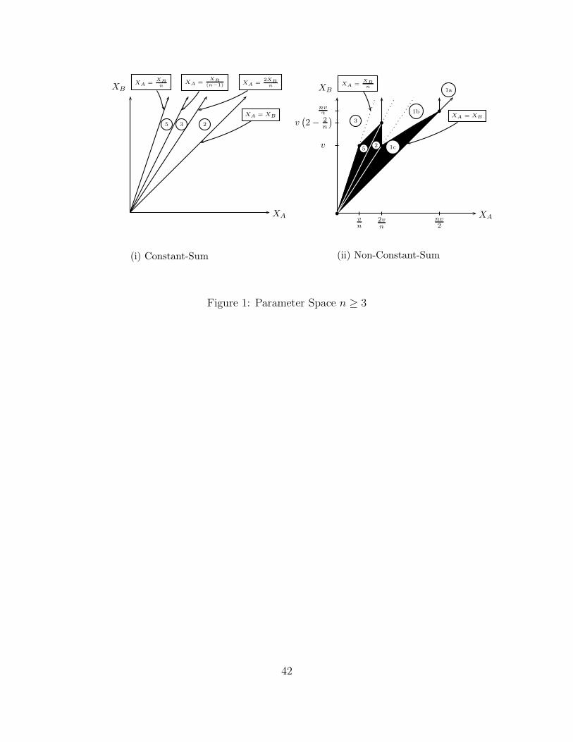
XA

XB

XA = XB

XA =2XB

nXA =

XB

(n−1)XA =XB

n

235

(i) Constant-Sum

XA

XB

v

nv2

v(2− 2

n

)

2vn

vn

nv2

XA =XB

n

XA = XB

1b

1a

1c

3

52

b

b

b

b

b

(ii) Non-Constant-Sum

Figure 1: Parameter Space n ≥ 3

42

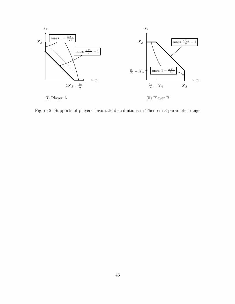
x1

x2

XA

2XA − 2vn

mass 1− nXA

2v

mass nXA

v − 1

(i) Player A

x1

x2

XA

2vn −XA

XA2vn −XA

mass 1− nXA

2v

mass nXA

v − 1

(ii) Player B

Figure 2: Supports of players’ bivariate distributions in Theorem 3 parameter range

43

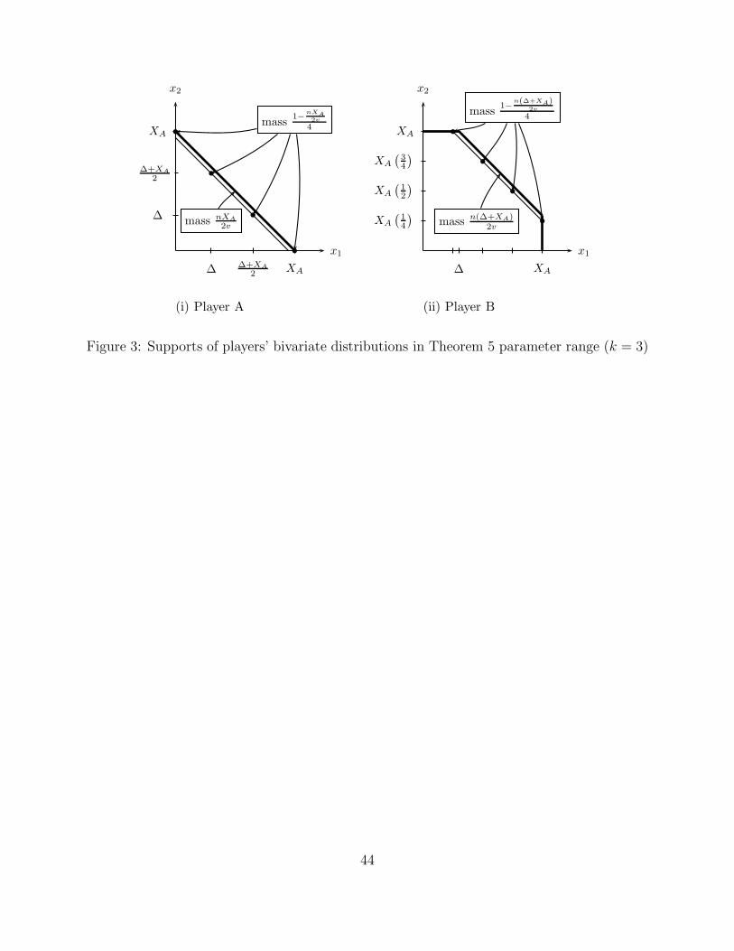
x1

x2

XA

∆+XA

2

∆

∆+XA

2∆ XA

mass1−

nXA

2v

4

mass nXA

2v

b

b

b

b

(i) Player A

x1

x2

XA

XA

(12

)XA

(34

)

XA

(14

)

XA∆

mass1−

n(∆+XA)2v

4

mass n(∆+XA)2v

b

b

b

b

(ii) Player B

Figure 3: Supports of players’ bivariate distributions in Theorem 5 parameter range (k = 3)

44

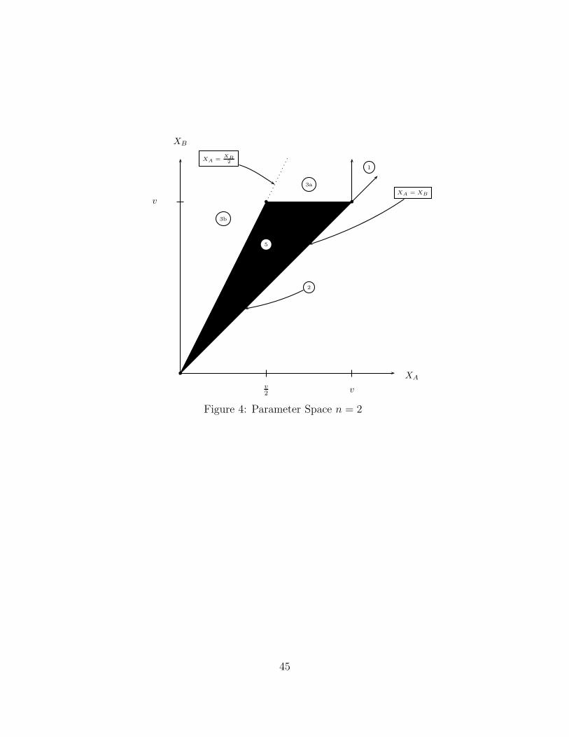
XA

XB

v

v2 v

XA = XB

1

2

XA =XB2

3b

3a

5

b

b b

Figure 4: Parameter Space n = 2

45