Working Paper #03-03 (02) Business Economics Series January 2003

Sección de Organización de Empresas de Getafe Universidad Carlos III de Madrid

Calle Madrid, 126 28903 Getafe (Spain) Fax (34) 91 624 5707

THE NINETIES IN SPAIN: TOO MUCH FLEXIBILITY IN THE YOUTH LABOUR MARKET?*

J. Ignacio García-Pérez1 and Fernando Muñoz-Bullón2

Abstract This paper examines movements into and out of employment in the Spanish youth labour market throughout the nineties. We analyze how differences in personal and economic circumstances influence such movements. In addition, we consider the importance of duration dependence in determining them. Our main findings are that: (i) Very young workers, women and those with lower qualification levels are more likely to be affected by high labour turnover; (ii) The existence of unobserved heterogeneity has important consequences in the unemployment hazard rate; (iii) In the 90's, employment hazard rates were substantially affected by the extensive use of fixed-term contracts, although the 1997 labour market reform seems to have reduced this hazard rate; (iv) The intervention of temporary help agencies has a positive impact on the likelihood of leaving unemployment, although only for short-term unemployed individuals; at the same time, however, the employment hazard rate is substantially higher within these agencies. Keywords: employment and unemployment hazard rates; duration dependence; unobserved heterogeneity; temporary help agencies. * This work has benefited from financial support by CICYT SEC2002-04471-C02-02. We would like to express our gratitude to the Spanish Ministry of Labour for providing the database for this research, and to the seminar participants at IV Jornadas de Economía Laboral (Valencia), XXVI Simposio de Análisis Económico (Alicante), U. Santiago, U. Toulouse, U. Pompeu Fabra, the Workshop on Job Stability and Security in European Labor Markets (IZA, Bonn) and the XIV EALE Conference (Paris) for valuable suggestions. The usual disclaimer applies. 1centrA:, C/ Bailen, 50 - 41001 Seville (Spain). E-mail: jigarcia@fundacion-centra.org 2Sección de Organización de Empresas. Universidad Carlos III de Madrid. C/ Madrid, 126. 28903 Getafe (Madrid). E-mail: fmunoz@emp.uc3m.es

1 Introduction

The Spanish labour market has traditionally been perceived as a very rigidone for two principal reasons. Firstly, unemployment rates are persistentat very high levels: whilst unemployment increases in recessions, it doesnot reduce su¢ciently in periods of economic growth. Secondly, the lengthof time that an individual tends to be unemployed for is also very long.Subsequently, the proportion of long–term unemployment has become moreimportant, even in periods of intense economic growth. For instance, from1987 to 1991, around 57.4 percent of those who were unemployed in Spainwere so for more than one year. Throughout the nineties, this percentagehas been around 52.7 percent.

In spite of this, we may wonder if the Spanish labour market is, indeed,so rigid. In 1984, the Spanish government implemented a huge liberalizationof employment protection regulation by allowing the extensive use of …xed-term or temporary labour contracts. Following this reform, employment inSpain has grown principally due to temporary contracts (they represent morethan 90% of new hires). In the nineties, the proportion of temporary workershas always remained above 30%, the highest level in Europe. Moreover, theduration of these temporary contracts has typically been very short. In1999, more than 58% of the total number of temporary contracts were forless than one year (31% were for less than one month). These facts aretotally at odds with the previous impression of a rigid labour market.

In order to investigate the degree of ‡exibility in the Spanish labourmarket, it is essential to study how many individuals are changing their sit-uation at a given moment1. This paper focuses upon this issue by examiningmobility patterns in Spain over the last decade. In particular, we investi-gate the determinants of employment and unemployment hazard rates, usinga sample of over 19,000 individuals a¢liated to the Social Security system.This sample consists of the whole labour history of workers who were, at theend of 1995, either employed through a Temporary Help Agency (THA) ornon-employed in this month. Hence, given that these agencies hires mainlyyoung workers (83.6% of the labour contracts signed by THAs were withworkers under 35 years-old), the data set is only representative of youngworkers in the Spanish labour market. Thus, our analysis is intended toprovide information on mobility rates for young individuals over a long timeperiod (1990 to 1999). These individuals constitute a group of much con-cern for policy in Spain, given that 59.19% of the unemployed and 80.81% of

1 Such an analysis is of considerable importance, because the existence of high rates ofunemployment in Spain may be hiding important in‡ows and out‡ows from unemploymentto employment. See, for instance, García–Pérez (1997).

1

temporary contracts belonged to workers under 40 years-old in this period.We use duration models applied to a longitudinal data set on individ-

uals’ work history by taking into account the e¤ects of both duration andindividual heterogeneity in the hazard or exit rates. Our estimation tech-nique allows us to take account of concurrent events via time–dependentvariables, similar to the ones used in Bover, Arellano and Bentolila (2002)and García–Pérez (1997). In addition, given that some variables which maya¤ect both employment and unemployment duration (e.g., family income,skills or unemployment bene…ts) are unobserved in our data set, it becomesnecessary to control for the presence of unobserved heterogeneity. The useof Social Security records presents certain advantages for the analysis ofturnover with respect to other sources of information2. Firstly, it collectsinformation on all jobs held. Secondly, it allows us to determine employ-ment and non–employment durations precisely. Di¤erent statistical sourceshave also been used to study the determinants of employment transitions;in particular, we can mention the use of the 1985 Encuesta de Condicionesde Vida y Trabajo by Alba–Ramirez (1991), Andrés et al. (1989), SánchezMoreno and Peraita (1996) or García–Serrano and Malo (1996), and the useof the Spanish Labour Force Survey by Toharia (1996, 1997), and Bover etal. (2002). With regards to ‡exibility, we can conclude from these studiesthat, during the time-periods analyzed, there has been an increase in in‡owsand out‡ows between unemployment and employment.

However, to our knowledge, there is no research on mobility patterns inSpain for the period 1990–99, where we observe two moments of equal ex-pansion, 1990 and 1997, and a big depression in the middle, 1993. This timeperiod is also of considerable importance, since, throughout the nineties,the observed bad functioning of …xed-term contracts, along with the un-employment rate —at over 20 percent of the labour force— triggered theimplementation of two main labour market reforms in 1994 and 1997.3 The1994 reform put forward speci…c limits on the use of …xed–term contracts:the minimum and maximum duration of temporary contracts for young peo-ple were changed to 6 months and 2 years, respectively. It also extendedthe subsidies and incentives to promote the conversion of …xed–term con-tracts into permanent ones which were introduced in 1992. The 1997 reformimplemented again new measures that attempted to rectify the excessiveprecariousness present after 1984: more subsidies to promote the transi-tion from temporary to permanent contracts were agreed upon and a newtypology of permanent contract with lower …ring costs targeted at “pro-tected categories” of workers —young people under 30 years–old, long–term

2 A di¤erent extraction from Social Security records was previously used to study em-ployment and unemployment spells through the use of duration models in García–Fontesand Hopenhayn (1996) and García–Pérez (1997).

3 See, for example, Güell and Petrongolo (2000) or Segura(2001) for a deep descriptionof these reforms.

2

unemployed, people above 45 years–old and disabled individuals— was in-troduced. Given this new institutional context, we consider the analysis ofboth in‡ows and out‡ows from employment in this decade essential in the as-sessment of whether di¤erent mobility patterns. In particular, we make useof well-known econometric models for duration analysis in order to evaluatethese Government policy changes that have occurred along the nineties.

From our results we …nd that the exit rates from both employment andunemployment are very high. This leads us to the conclusion that there hasbeen a high level of ‡exibility in the Spanish youth labour market through-out the 90’s. The use of …xed-term labour contracts is widespread. More-over, very few of these contracts are renewed as permanent ones, whichleads again to the persistence of turnover rates, especially for very young,low quali…ed individuals and during recession periods. These facts are likelyto be the reasons why the exit rate from employment presents a very im-portant peak exactly at the thirty-sixth month, the maximum duration of a…xed-term contract in Spain. We have also obtained evidence that supportsthe argument that the 1997 labour market reform reduced the high turnoverrates observed in the central years of this decade. From information on thetype of contract held by individuals, we are able to conclude that the newtype of permanent contract introduced with the 1997 reform has substan-tially improved the probability of …nding and maintaining employment.

The paper is organized as follows. Firstly, we summarize the factors un-derlying the duration of both employment and unemployment spells. Sec-ondly, we show the econometric models for duration analysis that we usein our estimations. We then describe the data in detail and subsequentlypresent the empirical results. The last section o¤ers our conclusions.

2 Framework of analysis

2.1 The duration of unemployment spells

The theoretical analysis of unemployment duration is based on job searchmodels (see extensive surveys in Mortensen, 1986 or Devine and Kiefer,1991). The basic outcome of these models is the unemployment hazardrate. This hazard rate is the product of the probability ®(t) of receivinga job o¤er and the probability that the non–working individual will acceptthe o¤er. The latter is the probability that the arriving wage o¤er is higherthan a critical value, called the reservation wage, wR(t).

The job o¤er probability, ®(t); is a function of both the level of demandand the search activity of job seekers. In this sense, an individual’s level ofquali…cation can be expected to have a positive e¤ect on ®(t); a negativeimpact of age is expected as well. As regards the intensity of search, it isevident that it must have a positive impact on ®(t). Finally, employmentdemand conditions —measured either through the unemployment rate or

3

through the number of vacancies— may be having some in‡uence on ®(t)in the sense that the better those conditions are, the higher the expectedjob o¤er probability. Apart from these main e¤ects, we can expect this o¤erarrival rate to vary with the duration of the unemployment spell. Di¤erenttheoretical models predict a negative duration-dependence of this arrivalrate based, for instance, on human capital depreciation or stigma e¤ectsappearing as unemployment lengthens.4

The other component of the unemployment hazard rate is the acceptanceprobability which is equal to the probability that the o¤ered wage is equal orhigher than the reservation wage. Therefore, any variable which increases (orreduces) the reservation wage will reduce (or increase) the job acceptanceprobability and, in addition, will reduce (or increase) the probability ofexiting from unemployment, given all other things equal. Hence, the e¤ectof variables that increase income while unemployed, for example the receiptof unemployment bene…ts, will clearly raise the reservation wage, reducingthe unemployment hazard rate.

Finally, as well as the arrival rate, and in part because of it, the reser-vation wage is also a function of unemployment duration. For instance, theamount of unemployment bene…ts received is not constant along time, butdepends on its duration; moreover, search intensity may be attenuated asunemployment goes on. All these factors make the reservation wage de-crease with unemployment duration. But this also causes the acceptanceprobability to increase and, hence, no clear prediction arises for the e¤ectof unemployment duration on the unemployment hazard rate. However,available empirical evidence indicates that, in general, the net e¤ect is nega-tive5 or positive at the beginning of the unemployment spell and decreasingafterwards (See García-Pérez, 1997, 2001b).

2.2 The duration of employment spells

The duration of employment spells has usually been analyzed using themodels of e¢cient labour turnover developed by Jovanovic (1979a,b). Theseare incomplete information models in which (i) workers’ abilities are not fullyknown at hiring; (ii) the employer would like to produce at a desired levelbut deviation from this level is acceptable so long as it does not fall belowa minimum threshold; and (iii) the …rm monitors workers until su¢cientinformation is collected in order to make a judgement with the acceptabledegree of accuracy. In this context of incomplete information, the actualcontract goes on as long as the individual’s expected productivity keepsabove a threshold …ring level (called the reservation productivity). Thus,the hazard rate out of employment is equal to the probability that thisexpected productivity falls below the reservation productivity.

4 See, for instance, Vishwanath (1989) or Pissarides (1992).5 See Narendranatham et al. (1985), and Nickell (1979).

4

Jovanovic’s model was designed for homogeneous workers. However,when estimating the hazard rate from employment, we must take into ac-count the observed di¤erences among workers. Those di¤erences may be dueto both individual or job position characteristics. With respect to the for-mer ones, workers with the most valued features for the …rm will have longeremployment spells. Secondly, some job position characteristics (such as therequired quali…cation level for the job) may a¤ect the employment hazardrates: a higher quali…cation can be associated to longer tenure in the …rm ifemployers consider that workers complying with higher quali…cation levelsare more ‡exible and have a higher ability of adaptation; In addition, thereservation productivity de…ned for worker–…rm matching may also dependon the economic cycle and on local labour market conditions.

Once we have taken into account the fact that di¤erent individuals havedi¤erent probabilities of exiting from employment (i.e., the heterogeneity ef-fect), we must also consider the possibility that these probabilities dependon the actual length of the employment spell (i.e., the duration e¤ect). Ac-cording to Jovanovic’s model (1979b) the likelihood of job ending is expectedto be shorter the longer the duration of the spell; the reason being that thoseindividuals who are “good matches” dedicate less time to …nd alternativeo¤ers and are less likely to accept any such potential o¤er. In addition, wewould also expect that, the longer the spell, the more important the invest-ments in speci…c human capital will be; the greater the speci…city of thisinvestment, the more likely the continuation of the worker–…rm match inthe future will be, so that the employment hazard rate diminishes. Anotherimportant factor is that the longer the employment spell, the higher the…ring costs. Hence the …rm will have less incentives to get rid of the worker.

3 Duration analysis: econometric proceedings

In order to study the hazard rate for both employment and unemploymentspells, a discrete-time duration model will be used. The estimation techniqueis similar to the one exploited in the works of Narendranathan and Stewart(1993), Sueyoshi (1995), Jenkins (1995), García–Pérez (1997) and Bover etal. (2002). The reason for using discrete–time techniques is not only thatdata are observed in discrete intervals (namely, in months) but also thatthese techniques are much more ‡exible for estimating the time–dependenceof the hazard rate (see Meyer, 1990).

Moreover, the technique used in this paper helps us to circumvent theusual assumption of proportionality between the e¤ects of duration andother covariates over the hazard rate. There are cases in which the impactof explanatory variables changes with duration in a determined state (forexample, in our case, the e¤ect of having been a THA-worker over the exitrate from unemployment may not be the same for the short as for the long-

5

term unemployed). Because of this, it becomes necessary to model thehazard rate in a non-proportional way and, for this purpose, discrete timehelps considerably.

Therefore, our hazard rate will be the following conditional probability:

µ(t) = Pr(T = tjT ¸ t) (1)

where, given that we are modelling a dichotomous variable, we can con-sider its dependence on duration and other explanatory variables througha known distribution function. As in other papers, for example García-Pérez (1997) or Bover et al. (2002), we will use the logistic distribution.Hence, considering the duration in employment and unemployment statesas our discrete random variables, and taking also into account the e¤ect ofpersonal characteristics, our two conditional exit rates will be as follows:

µ(t) = F (µ0(t) + µ1(t)x(t)) (2)

where x(t) is a vector of personal characteristics —which do not vary overtime— and of aggregated characteristics which do vary over time t; µ0(t) isthe additive term of the duration-dependence in the hazard rates that wewill estimate in the most general way; and µ1(t) represents the coe¢cientsfor the explanatory variables which in general depend on duration —that is,interactions between these variables and duration are allowed for.

Due to the absence in our data set of important determinants of bothhazards —some of them being, e.g., family income, characteristics of thejob and whether or not the individual is receiving unemployment bene…ts—and, given the known result of unobserved heterogeneity generating spu-rious duration-dependence in the hazard rate (see, for example, Flinn &Heckman, 1982), it becomes necessary to control for this problem. Hence,in the presence of unobserved heterogeneity, our hazard rates will have thefollowing form:

µ(t; ´) = F (µ0(t) + µ1(t)x(t) + ´) (3)

We do not wish to impose more structure upon our estimation. Thus, wewill follow a semi-parametric approach based on Heckman and Singer (1984)where we are assuming that unobserved heterogeneity follows a discretedistribution function with di¤erent mass points. In particular, our resultsare based on a two–mass–point distribution function.6

6 In addition, an alternative estimation with three di¤erent mass points was undertaken;however, one of them always converges to zero. Therefore, we believe that the distributionfunction with two mass points properly accounts for the unobserved heterogeneity in ourdata.

6

The estimation technique of the model is maximum likelihood. Given thelikelihood contribution of each individual i in the sample, Li(´); 7 conditionalon ´, we obtain that with unobserved heterogeneity, ´; the log-likelihoodfunction takes the form:

ln $h =NX

i=1

ln

ZLi(´)dF (´) (4)

where F (´) is the cumulative distribution function of ´; which is a discretefunction with two mass points, ´1 and ´2: These mass points are selectedin order to verify the assumption of E(´) = 0 which is necessary given thepresence of a constant term in the hazard rates. Besides, it is estimated theprobability p for the variable ´ to be equal to its value ´1: Hence, we willestimate all the parameters of the hazard rates, along with p and ´1:

4 Data

The data source are work histories of a sample of 19,778 individuals collectedfrom administrative data belonging to Social Security records. It includes in-formation on all individuals’ employment (and non-employment) spells from1990 to 1999 of a sample of mainly young workers.8 In fact, our data set isonly representative of young workers in the Spanish labour market. In par-ticular, workers from 20 to 35 years-old account for 49% of the total sample,while, according to the Labour Force Survey, those individuals represented32% of the active population in Spain at the end of 1995. Therefore, ourestimates can not be generalized to provide insights about the overall levelof job mobility in the economy. On the contrary, our analysis is intended toprovide information on mobility rates for young individuals over a ten-yearperiod, who constitute a group of much concern for policy in the Spanishlabour market.

The work history data provided includes information about worker ageand gender, professional category of the worker contribution to the SocialSecurity9, dates at which employment spells start and end, type of Social

7 See García-Pérez (1997) or Bover et al. (2002) for an expression of this likelihoodfunction.

8 This is due to the way the sample were obtained. It was selected 10.000 workers hiredthrough a Temporary Help Agency (THA) at the end of 1995 and the same number ofindividuals who were non-employed at this same date.

9 We must underscore that the eleven professional categories of worker contribution tothe Social Security in the database do not reveal the workers’ level of quali…cation, butrather the required level of quali…cation for the job. For instance, an individual working inthe lowest category, “peón”, may well be in possession of an academic degree. In any case,we will refer to contribution categories from here onwards as “quali…cation”, althoughthis remark should be taken into account for the subsequent analysis. As in previousstudies using data from the Social Security records, we group those eleven categories infour groups from maximum to minimum quali…cation required for the job.

7

Security system for the worker, the reasons for the termination of the spell(voluntary quit, dismissal or retirement), the Spanish province where theemployment spell took place, an identi…er indicating whether or not eachemployment spell is accomplished through a THA, another one if it is ac-complished through a public …rm, and, …nally, the type of contract held bythe worker (temporary or permanent). We eliminate incomplete records,and also spells of individuals above 52 years-old in order to avoid the biasthat early retirement programs may create in both exit rates, and keep onlyworkers a¢liated to the General System (Régimen General) so as to avoidthe bias in the estimations that special systems like Agriculture, Fisheries,and so on would provoke. In addition, given that mobility patterns arisingfrom quits are likely to substantially di¤er from involuntary separations, inorder to achieve greater homogeneity, we also eliminate records destroyed forreasons other than dismissals or end of contracts.10 Finally, given that wewant to use information about the following employer in each employmentor unemployment spells, we keep only individuals with at least two observedemployment spells11.

Our database contains an important number of individuals presentingsubsequent employment spells through the same …rm, with particularly shortunemployment spells in-between these jobs. Evidence for this is shown inTable 1. This table shows average employment and unemployment durationsfor individuals who present no subsequent spells through the same …rm, andfor individuals who, on the contrary, have from two to twelve consecutivespells through the same employer along their work history. Average employ-ment duration for the former equals 199.43 days. On the contrary, for thoseworkers with the same employer in the following spell, the average employ-ment duration is just 76.07 days. Moreover, job durations reduce quickly asthe number of spells through the same employer increases (from an averageduration of 136 days with only two spells with the same …rm to less than 16days when the number of consecutive spells is 12). Something similar occursfor unemployment spells: while the average stay in unemployment for thoseindividuals who have no spell through the same …rm in their work historyis 71.37 days, the average duration of these unemployment spells reducesas the number of unemployment spells in-between employment spells with

10 In this database we cannot distinguish between these two di¤erent reasons for termi-nation of the spell and, therefore, we consider both as involuntary turnover. Moreover,we will not consider voluntary turnover. As both reasons of terminating the employmentspell are totally di¤erent, we think they have to be studied separately. Hence, futureresearch will compare the results in this paper to the results arising from an analysis ofthe subsample of records ending in quits.

11 Given that the data set is mainly constituted by young workers, the percentage ofindividuals who do not hold at least two employment spells is insigni…cant. That is, whenwe keep individuals for whom only a single spell of employment is observed, the …nalsample is very similar to the one …nally used in the analysis. Statistics are available fromthe authors upon request.

8

the same …rm increases (so that on average, individuals who do have spellsthrough the same …rm only su¤er on average 20.71 days in unemployment).Therefore, the more likely the individual is to be employed through the sameemployer, the shorter the intermediate unemployment spells he must con-front with. This fact is re‡ecting the new hiring policies adopted by …rmswhich consist on using intensively very short temporary contracts in orderto avoid uncertainty and also, of course, to reduce labour costs.

Given this high turnover rate observed in our data —with mainly shortunemployment spells— and in order to avoid estimating transitions betweentwo di¤erent employment spells without passing through a real state of un-employment, we decided not to use either unemployment and employmentexperiences shorter than 15 days.12 The basic change these spells provokeover the employment hazard rate is that this is much higher at duration 1.In addition, estimations implemented with these spells show no special dif-ferences compared to the ones presented here. The only remarkable changeis that the THA e¤ect over the hazard rate becomes even stronger, giventhat many short–term jobs are implemented through these …rms.

As regards employment spells, our sample consists of 49,322 spells13,whose characteristics can be observed in Table 2. Our sample of estimationis composed mainly of relatively young males, with a reduced quali…cationlevel, and with very short durations in employment (indeed, more than halfof the observations in our database present durations of less than 3 months).Given that there is a very small number of observations for long durations(>46 months) and in order to avoid noise in the results, we have consid-ered these observations as arti…cially right-censored, that is, as employmentspells that do not …nish in the observed period. This is the reason why thereare no observations with employment durations beyond 46 months. In ad-dition, there are individuals who continued being employed at the momentin which the data were downloaded (December 1999); these observationsare also right–censored, because their spell was not complete at that mo-ment. However, most of jobs (95.75%) terminate during the sample period.As opposed to the sub-sample of non–THA individuals, workers who …ndemployment through these intermediaries are more likely to be younger, fe-male and to be in possession of a reduced quali…cation level. In addition,THA workers enjoy shorter employment durations than non–THA individ-uals (the average tenure is 3.65 months, as opposed to 6.09 months fornon–THA workers).

12 It is unknown whether very short spells are either true unemployment spells or justrepresent a delay in registering the worker at the Administration after a job–to–job move-ment.

13 This is a sub–sample of the initial sample (of 180,010 records); it was necessary to takethis random sample due to the techniques of estimation implemented. In the estimation,each (non)employment spell is broken down into so many monthly observations as theduration of the corresponding spell (See Jenkins, 1995).

9

We have a sample of 34,137 unemployment spells. Their main character-istics can be observed in Table 3. For the same reason as in the employmentanalysis, we consider unemployment durations beyond 30 months and theones that have not …nished before December 1999 as right-censored unem-ployment experiences. Again, in this sample of unemployment records, menare the majority; most of observations show low quali…cation levels; youngindividuals (under 25 years–old) represent almost half of the total samplesize, and only 15.42 percent of complete unemployment experiences lastedbeyond 6 months. As regards THA individuals when compared to non–THAones, we …nd that agency workers are more likely to be younger, in posses-sion of reduced quali…cation levels and to have shorter unemployment spells(the average stay in unemployment is of 2.81 months for agency workers,but 4.29 months for non–THA individuals).

Given the estimation technique used, which consists of breaking downthe event into monthly observations in which the individual is at risk offailure in employment or unemployment (see Jenkins, 1995), the …nal lengthof the database on employment and unemployment is of 311,156 and 146,071registers, respectively.

5 Estimation results

As explained in the previous section, a discrete-time duration model will beestimated for both employment and unemployment spells using a sample ofSpanish workers. The estimation results will be …rstly presented based onthe model without controlling for unobserved heterogeneity. Then, these re-sults will be compared to the ones obtained when controlling for the presenceof unobserved heterogeneity in both hazard rates.

The speci…cation of the hazard rates will be the following. Apart fromthe variables on individual and job characteristics, the business cycle and lo-cal economic conditions (which collect the observed heterogeneity e¤ect), theduration-dependence has been taken into account through the inclusion of apolynomial in log(t). In addition, dummy variables indicating whether or notthe individual is on–the–job in his sixth, twelfth, eighteenth, twenty–fourth,thirtieth or thirty–sixth month have been included in the employment haz-ard rate. We do this because, as explained below, evidence indicates thatthe likelihood of exiting from employment is signi…cantly higher in thesemonths. Finally, interactions between duration (in employment or unem-ployment) and some of the explanatory variables have also been speci…ed14.

14 The …nal speci…cation of the estimated models only presents the interactions that areobtained to be signi…cant. The initial speci…cation included all the possible interactionsbetween duration and the explanatory variables. Moreover, the shown polynomials inlog(t) are the ones which obtain the best results in terms of signi…cance and likelihoodvalues.

10

5.1 Hazard rate from employment

Let us …rst examine the e¤ect of employment duration on the likelihood ofexiting from the job. Monthly Kaplan–Meier estimates for the total sampleare plotted in Figure 1. This empirical hazard function collects the propor-tion of individuals leaving employment at each moment in time, given thatthey have been employed until that moment (Lancaster, 1990).

As can be observed, this hazard rate is declining with employment du-ration, so that the probability of job ending declines with tenure on the job.The exit rate is clearly very high early in the job, reaching 32.62% in the…rst month; it falls to 5.61% at the end of the …rst year, and then remains ataround 3% from then on. However, the most interesting result in Figure 1 isthe fact that the hazard rate actually rises to peaks in months 6 (32.34%),12 (19.07%), 18 (12.27%), 24 (16.70%), 30 (12.46%) and 36 (32.47%). Thesepeaks show that job contracts are very likely to …nish at each of these par-ticular months. This fact can be explained, basically, by the extensive useof …xed-term contracts which are usually for these speci…c durations.

In Table 4, we present the results of the maximum likelihood estimationof the hazard rate out of employment assuming a logistic distribution for F(equation 3), under the two assumptions of no unobserved heterogeneity anda two–mass–point distribution function for this heterogeneity. As expectedfrom the shape of the empirical hazard rate previously presented, tenure onthe job presents a negative impact on the exit rate. That is, individuals whohave been employed for longer are less likely to exit from the job. Moreover,the dummies describing employment durations which are multiples of six(i.e., durations of 6, 12, 18, 24, 30 and 36 months) present a positive andvery signi…cant e¤ect on the hazard rate. Since in this database it is notpossible to distinguish as a reason for termination of the spell, between theend of a temporary contract and a dismissal, and, given that no specialreason can be adduced to explain why individuals should be dismissed atthose months multiple of six, we can then deduce that the positive e¤ectof these dummy variables must be very likely due to temporary contractterminations. These e¤ects can be quali…ed by taking into account thesedummies’ interactions with some of the factors collecting the heterogeneitye¤ect. Hence, for instance, we obtain that higher rates of economic growthreduce the likelihood of exiting from employment at those peak months,presumably re‡ecting that better economic conditions encourage the signingof permanent contracts (instead of temporary contracts). Moreover, youngerindividuals and those not working in public …rms are the most likely to su¤erfrom contract termination at those months.

Let us examine the e¤ects of other factors (apart from the actual du-ration of the spell) on the likelihood of exiting from employment. We willbegin by considering the e¤ect of individual’s job position. The …rst resultis that those individuals who are working through a THA are more likely to

11

experiment shorter employment spells15. This THA e¤ect can be observedin Figure 2, where it can be noted that THA workers also show strongerpeak-month e¤ects. These results are sensible when considering both thedemand and supply–side motivations for addressing to THAs16. From thedemand–side, those intermediaries are often used as a “bu¤er” for client…rms in order to meet changes in the product demand in a context where…rms are reluctant to hire permanent sta¤ until the economic outlook be-comes more stable. From the supply–side, workers addressing to THAs oftenappreciate the limited work hours or the greater ‡exibility in scheduling thatcan typically be found in these …rms. Therefore, THA workers are expectedto show shorter durations in employment (see Table 2).

In Table 5, we have the predicted average durations in employment fordi¤erent groups of individuals distinguishing between their age, sex andquali…cation level. We can see that the whole sample’s predicted employ-ment duration is 6.35 months and that this predicted duration is much largerfor no-THA workers. However, we …nd that both male and female skilledworkers with less than 25 years of age present larger expected employmentdurations under THAs. Hence, it seems that THAs could be doing a goodjob with very young skilled workers.

A positive impact on the employment hazard rate appears when theemployer in the following employment spell is the same as the presentone (so-called equal employer). One of the reasons why individuals whoare contracted by the same employer are more likely to enter into unem-ployment might be due to the hiring policy adopted by …rms; the lattermay resort to former employees in order to …ll vacancies. Thus, employersmay be temporarily …ring workers —with whom they have no permanentcommitments— during periods of low demand or in order to avoid having topay fringe bene…ts (such as, for instance, holiday pay); then, once two weekshave passed after the …ring decision, those same former workers are then ac-tually rehired. Finally, a positive impact on the hazard is also obtainedwhen the individual has been employed through a public …rm, although theimpact is lower as experience in the job lengthens.

With respect to the e¤ects of worker’s characteristics on the probabilityof leaving employment, at the beginning of the employment spell, men areless likely to exit from employment than their female counterparts, althoughthis di¤erential gender impact is reversed the longer the duration of the spell.

The employment hazard rate is higher for the young (people under 26years–old). They also show substantially higher exit rates especially at peak-months. This result presumably indicates lower …rm costs when laying o¤these workers, given the temporary nature of many of the contracts that

15 There might exist selection by workers into THAs. This bias can be taken into accountby jointly estimating a process for the decision of whether or not to work for a THA. Thisanalysis is being undertaken by the authors in a companion paper.

16 See Muñoz–Bullón, 2002.

12

they hold. Finally, as expected, very low levels of quali…cation increasesubstantially the probability of exiting employment (see Figure 3).

The e¤ect of economic conditions on the probability of entering intounemployment is showed in Figure 4. This …gure plots the combined e¤ectof the local unemployment rate and that of the GDP growth rate at themoments where the GDP attains its maximum and minimum values for our10–year period of observation; the average values of unemployment rates arealso taken into account at the two extreme cyclical points. The employmenthazard rate is counter-cyclical only for short employment spells, those ofless than 5 months. This result makes sense, since, when things are gettingworse, …rms are dismissing workers whose on–the–job experience is shorter.

Finally, we have included two additional dummies in our estimation toallow for the speci…c impact of three distinctive periods throughout thenineties. In order to capture the potential e¤ect of the two labour marketreforms in this decade, we make distinctions between the spells observedbefore 1995, then those between 1995 and 1996 —that is, under the e¤ect ofthe 1994 reform— and, …nally, those spells from 1997 onwards —which mayshow a di¤erent behavior on the hazard rate as a result of the 1997 labourmarket reform. Net of the business cycle e¤ect, we …nd that both periodsshow higher employment hazard rates than those at the beginning of thenineties. However, the e¤ect changes with tenure and with the impact ofindividual variables. As regards tenure, for both the period from 1995-1996and the period after 1997, this positive e¤ect is reduced the longer tenuresare. Hazard rates in both periods are also reduced the higher the GDPgrowth rates are. As regards the impact of individual variables, the highemployment hazard rates obtained for the period 1995-96 are even largerfor the low-quali…ed youngest individuals (under 36 years-old) and for thoseworking through a public …rm. As for the speci…c e¤ect of the period 1997-onwards, the hazard is specially higher for low quali…ed individuals and thoseabove 36 years-old. This e¤ect may well show the reduction of turnover foryoung people after the 1997 labour market reform. The complete e¤ect ofthese two dummies can be better understood in Figure 5. The employmenthazard rate is the highest in the period 1995-1996. Initially, the estimatedhazard rate for 1990-94 is the lowest one; however, note that for tenure onthe job above nine months, the lowest hazard rates are always obtained forthe period 1997-99. We may, therefore, conclude that, in spite of the factthat …ring rates increased after the 1994 reform, they were inferior to theirinitial levels after the implementation of the 1997 reform. In addition, theespecially high …ring rates characteristic of peak–months clearly decreasedfrom 1997 onwards.17 While exercising caution with these dummies —whichmight be in‡uenced by other potential e¤ects— it seems that the labour

17 Of course, we have no data for employment spells larger than 24 months in the period1997-1999, so the estimations for the duration dependence after that month are obtainedsolely with the spells terminated before 1996.

13

market reform in 1997 slightly reduced the large turnover rates characteristicof the mid-nineties.18

In Table 5 we observed that the average employment durations predictedby our estimation are much lower after the 1994 labour market reform butthey recovered a bit after the 1997 one. In fact all age groups of skilledmales and very young skilled women were the mostly bene…ciated by thislabour market reform.

The last two columns of Table 4 show the estimation of a similar spec-i…cation for the employment hazard rate but, this time, controlling for thepresence of unobserved heterogeneity. We obtain no evidence in favor of thepresence of unobserved heterogeneity in our data. Although the likelihoodfunction is a bit higher when controlling for unobserved heterogeneity, weestimate almost one point in its distribution function (its value is not sig-ni…cant and has a probability of 0.9925). Hence, we can conclude that theemployment hazard rate may be accurately estimated without taking intoaccount the control for unobserved heterogeneity.

5.2 Hazard rate from unemployment

Empirical hazard rates from unemployment are shown in Figure 6. As pre-viously outlined, the maximum duration is of 30 months due to the scarcityof observations beyond this duration. The hazard rate begins an increas-ing trend from the very beginning of the unemployment experience, reachinglevels above 35 percent for the second month.19 However, it falls very quicklyuntil the eighth month, then shows another peak at the tenth month, and,from then on, remains at levels slightly above 5 percent.

Table 6 collects the results of the maximum likelihood estimation of theunemployment hazard rate assuming a logistic distribution for F (equation3). As before, we …rstly present the duration-dependence of the hazardrate in a polynomial for the logarithm of unemployment duration, and withinteraction terms between the remainder explanatory variables and unem-ployment duration. In particular, the additive term of the hazard rate col-lects a fourth–grade polynomial which replicates quite well the form of theempirical hazard rates.

Let us examine the e¤ect of di¤erent factors on the likelihood of exitingfrom unemployment. We shall begin by considering the e¤ects of workercharacteristics. Although the gender e¤ect is attenuated as length in un-employment increases, women are expected to su¤er longer durations inunemployment; this gender e¤ect may be justi…ed by recognizing that, in

18 We will later present a di¤erent estimation with a sub-sample of workers who gaveinformation about the type of contract held on the job in order to investigate more aboutthe new contracts introduced in this reform.

19 The smaller hazard rate at one month is simply a consequence of obviating unemploy-ment spells shorter than 14 days.

14

spite of the fact that the participation of women in the labour force hasbeen increasing from the 80’s on, it is still basically men who support theirfamilies. If this is the case, then, women —specially those with a workingspouse— may presumably be less likely to accept job o¤ers (See Ahn andGarcía-Pérez, 2002). As regards quali…cation, it is the individuals in thelowest group who are the least likely to exit from unemployment, while theones in the Medium-Low group are the most likely, followed by the mostquali…ed workers. Finally, workers in the medium age range (from 26 to 35years–old) are the ones who confront the shortest expected unemploymentdurations, though at a decreasing rate.

As regards the e¤ect of individual job position on the probability of leav-ing unemployment, having worked through a THA in the last employmentexperience represents a positive impact on the hazard rate, although theimpact is attenuated as unemployment lengthens. Why do previous em-ployment experiences through THAs represent an opportunity for quicklyleaving unemployment? There are at least two explanations for this result.Firstly, it could be that these intermediaries provide workers a better connec-tion to the labour force and, thus, greater access to information. Secondly,positions covered by client …rms through THAs are typically “assessmentpositions” in which performance is visible to a number of higher–level per-sons in the organization and in which performance largely determines futurecareer mobility; therefore, these observations and skill development charac-teristics of the THA positions increase the probability that capable peoplewill be engaged in permanent positions20. It makes sense then that thoseindividuals who stay unemployed for longer after a THA employment ex-perience become less attractive for potential employers (they may emit anegative signal to the latter). These e¤ects are re‡ected in Figure 7 wherewe …nd that the positive impact of having worked through a THA is onlypresent for those unemployed for less than four months.

In Table 7 we present the corresponding predicted unemployment dura-tions deduced from our estimations. Mean unemployment duration is 3.08months being a bit larger this duration for no-THA workers. However, itseems that skilled workers previously working through THAs su¤er longerunemployment spells than no-THA ones. Hence, although they are moretime in the job (remember Table 5), once they are unemployed, if theydo not exit quickly from this state, they could be sending a bad signal toemployers, thus having longer unemployment spells.

Experience in the previous employment positively a¤ects the probabilityof exiting from unemployment, though at a decreasing rate. This resultindicates that longer previous labour experiences raise the probability ofreceiving a job o¤er, especially at the beginning of the unemployment spell,

20 As Muñoz–Bullón (2002) indicates, hiring THA workers to monitor them and then too¤er permanent positions only to those who perform well seems to have become a commonstrategy of employers.

15

in spite of the fact that longer experiences are likely to be correlated withhigher unemployment bene…ts, which will probably reduce the likelihoodof accepting any job o¤er. Finally, if the …rm that hires the unemployedworker is the same as in the previous job, equal employer, the probabilityof exiting from unemployment is much greater. This “recall” phenomenonpreviously described is common in the labour market transitions re‡ectedin our empirical analysis. In addition, those individuals who have beenpreviously employed by a public …rm are more likely to stay for longer inunemployment.

As regards the e¤ect of economic conditions, the unemployment hazardrate is clearly pro-cyclical: higher levels of national economic activity showa positive e¤ect on the likelihood of exiting from unemployment. The com-bined e¤ect of the provincial unemployment rates and the GDP growth rateare shown in Figure 8 where we show the predicted hazard rate evaluatedat the moments of maximum and minimum GDP growth along with theaverage values of unemployment rates at those two extreme cyclical points.

Finally, and as in the case of the employment hazard rate, we have in-cluded two dummies in our unemployment estimation to allow for the spe-ci…c impact of three di¤erent periods during the nineties: 1990-94, 1995-96,1997-99. Net of the business cycle e¤ect, the impact of the dummies indi-cates that the e¤ect of the two labour market reforms is positive. Thereforethe likelihood of exiting from unemployment is higher in the second halfthan in the …rst half of the nineties. However, the e¤ect changes when wetake into consideration unemployment duration and the impact of individualvariables. The di¤erential impact of the period 1995-96 increases the longerthe unemployment spell is; a contrary impact of unemployment duration isobtained for the period 1997-99. The complete e¤ect of these two dummiescan be better understood in Figure 9 where we can see that the probabilityof leaving unemployment is maximum after 1997 only for those who stayedunemployed for less than 3 months. The e¤ects of GDP growth rate is not sopro-cyclical in the periods 1995-96 and 1997-onwards. As regards the impactof individual variables, the e¤ects of those two periods are also attenuatedfor individuals in the Medium-Low quali…cation group; on the contrary, theimpact is larger for the youngest (under 25 years-old). As for speci…c e¤ects,we …nd that the impact of the 1995-96 period is lower for individuals whohave been previously employed for longer and if they have worked througha THA. As regards the 1997-99 period, the e¤ect is increased for men andis reduced if they …nd employment with the same previous employer.

In Table 6, we can see that average unemployment duration clearly re-duced after the 1994 reform, specially for very young skilled workers. Afterthe 1997 reform, the average unemployment duration reduced a bit more butonly for unskilled workers under 25 years old and also for women between26 and 35 years old.

The presence of unobserved heterogeneity calls for an adequate control,

16

especially due to the absence of important determinants of the unemploy-ment hazard rate: apart from information about the household and thelabour market in which the unemployed worker is searching, the receiptof unemployment bene…ts is another important variable missing from ourdata.21 In order to control for this problem, we will use the same techniqueas before: we will assume that unobserved heterogeneity can be summarizedby a discrete two–mass–point distribution function.

Results from this estimation are shown in the last two columns of Table5. The estimated distribution function shows the existence of two di¤erenttypes of workers: with 22.56 percent probability, there exists a group ofworkers with a much higher unemployment hazard rate. The two estimatedtypes, in terms of hazard rates, are shown in Figure 10. Even though itis not possible to identify which speci…c characteristics lead to this result,unemployment bene…ts are likely to represent an important determinant.The e¤ects of unobserved heterogeneity over the remainder estimated pa-rameters are not very relevant since the estimated coe¢cients remain verysimilar. The only remarkable di¤erence is that under the control of unob-served heterogeneity, the duration-dependence of the unemployment hazardrate is less negative.

To sum up, medium–aged workers, males, relatively quali…ed workersand those working through a Temporary Help Agency —although the latteronly for very short durations in unemployment— enjoy higher chances ofexiting from unemployment. Moreover, given the previous result of contra-cyclical employment hazard rates for short employment durations, we cano¤er an explanation for the strong growth of the unemployment rate in thelast recession period of the Spanish economy: the extension of job destruc-tion, specially of short-term jobs, coupled with a very low exit rate fromunemployment in recession years make up two important factors for thesharp increase in this aggregate …gure.

6 Conclusion

The present paper has provided a basis for assessing the employment mo-bility patterns throughout the youth Spanish labour market in the nineties,a decade so far characterized by the lack of information about these labourmarket outcomes. We have set out the empirical results for the determinantsof employment and unemployment exit rates compiled from a representativesample of over 19,000 individuals a¢liated to Social Security. The time-spanof our analysis is of considerable importance, since the limits imposed during

21 In spite of this lack of information as regards this variable, given that the proportionof young workers that we have in our database is very high (as we will see below), andthat these individuals are less likely to be entitled to unemployment bene…ts, given theirshorter accumulated tenure. We think this lack of information is not so serious. In anycase, we have no means of contrasting this hypothesis.

17

the 90’s on the use of …xed–term contracts might have changed the pictureof transitions patterns sustained through previous empirical studies.

Our principal …nding is that employment and unemployment hazardrates are much higher in the 90’s than in the 80’s. In other words, throughoutthe nineties, the Spanish labour market has been even more ‡exible thanin the eighties. Temporary work through …xed–term contracts rather thanpermanent employment is responsive for these high turnover rates.

Within this overall picture of the labour market, there are many …ner ad-ditional results which are encountered with our empirical analysis. Firstly,we …nd that the probability of exiting from employment is negatively a¤ectedby job tenure and is largely determined by the duration of …xed–term con-tracts. Moreover, those with relatively low quali…cation levels and youngerwomen working through THAs are more likely to become unemployed. Sec-ondly, we …nd that a long duration of unemployment reduces the likelihoodof …nding a job, even when unobserved heterogeneity is controlled for. Inaddition, this hazard rate di¤ers according to the individuals considered:middle-aged men who have a intermediate quali…cation level and are at thebeginning of their unemployment spells are the most likely to re-enter em-ployment. Finally, and not surprisingly, the better the general economicconditions, the more successful individuals are in leaving unemployment.

We …nd that the existence of certain employment practices are also high-lighted by our results. For instance, employers are frequently resorting tolayo¤s and recalls. These are arrangements whereby workers are required tostop working for a temporary period —during which unemployment bene-…ts could be received— and after which they are re-employed by the same…rm. In addition, the practice of hiring workers through private employmentagencies seems to imply a trade–o¤ for the employee: For although this formof intermediated work implies enhanced opportunities of employment, theseworkers are only recruited for very short periods of time.

Finally, in spite of the fact that turnover rates in the nineties are excep-tionally high, some evidence is found to support the idea that the Govern-ment measures of 1997 —intended to tighten regulations governing tempo-rary work— have had some in‡uence on labour mobility patterns. For, thelikelihood of exiting from employment has reduced since 1997, and is partic-ularly lower in the months when temporary contracts …nish when comparedto the years 1990-1994 and 1995-1996. But at the same time, the likelihoodof exiting from unemployment is comparatively higher from the year 1997onwards when compared to the …rst decade of the nineties, although this isonly true for very short unemployment durations.

Additional evidence on the e¤ect of this labour market reform can bededuced from Table 8. This table shows (both for the employment and theunemployment hazard rates) the odds–ratios of the impact of four variablesrelated to the type of employment contract held, namely: permanent con-tracts, part-time contracts, the new, post-1997, permanent contracts, and

18

others resulting from the conversion of temporary contracts into permanentones.22 The most important results from this table are as follows.23 Withregard to the employment hazard rate, those individuals in possession of apermanent contract enjoy a 60.33% lower probability of losing their job. Fur-thermore, those holding a part–time contract su¤er a 41.12% higher proba-bility of exiting from employment than those holding a full-time temporarycontract. With regard to the unemployment hazard rate, those individualswho had held a permanent or part–time contract prior to their being un-employed …nd it comparatively more di¢cult to …nd a new job. Conversely,the unemployed who have previously been contracted through the new 1997permanent contracts show a 53.91% lower employment hazard rate at thesame time that it is found a much higher probability of leaving unemploy-ment. Hence, we think this is evidence showing that workers with thesenew permanent contracts have largely escaped the e¤ects of high turnoverrates in the nineties and they also maintain better chances of quickly leav-ing unemployment. Finally, we …nd no clear evidence on the e¤ect of theconversion of …xed-term contracts into permanent ones over both hazardrates. Hence, we can conclude that the principal bene…t of the 1997 reformcomes from the introduction of the new permanent contract. Whether thisis due to the reduction in …ring costs or the important subsidies received byemployers is a question that remains as yet unanswered.24

22 See the introduction for a more detailed explanation of this reform.23 The size of each subsample is lower due to the fact that some observations lack infor-

mation regarding contract type.24 We have estimated a speci…c model for only permanent workers, distinguishing those

with the new 1997 permanent contract from those under the former one. We …nd clearevidence that, under the new contract, the employment hazard rate is much lower thanfor those with the old permanent contract in the …rst year of tenure. Hence, we think thatit is not only the subsidies both contracts are receiving. It seems that the reduction in…ring costs could be under the fact that …rms are changing their …ring decisions early inthe job given its associated cost is lower under the new permanent contract.

19

References

[1] Ahn, N. and J.I. García-Pérez, (2002), “Unemployment Duration andWorkers’ Wage Aspiration in Spain”, forthcoming in the Spanish Eco-nomic Review.

[2] Alba–Ramírez, A. (1991). “Mismatch in the Spanish Labor Market:Overeducation?”. The Journal of Human Resources, 28, pp. 259–278.

[3] Andrés, J.; García, J. and Jimenez, S. (1989). “La incidencia y la du-ración del desempleo masculino en España”. Moneda y Crédito, vol.189, pp. 75–124.

[4] Blanco, J.M. (1995). “La duración del desempleo en España”, pp. 123–145, in J.J. Dolado and J.F. Jimeno (comps), Estudios sobre el fun-cionamiento del mercado de trabajo español, FEDEA, Madrid.

[5] Bover, O.; Arellano, M. and Bentolila, S. (2002). “Unemployment Du-ration, Bene…t Duration and the business cycle”, forthcoming in theEconomic Journal.

[6] Devine, T. J. and N.M. Kiefer (1991). Empirical Labor Economics: TheSearch Approach, Oxford University Press, New York.

[7] Flinn C.J. and J.J. Heckman (1982). “Econometrics Methods of Analyz-ing Labor Force Dynamics”, Journal of Econometrics, 18, pp. 115-168.

[8] García–Fontes, W. and H.Hopenhayn (1996). “Flexibilización y Volatil-idad del Empleo”. Moneda y Crédito, vol. 201, pp. 205-227.

[9] García-Pérez, J. I. (1997), “Las Tasas de Salida del Empleo y el De-sempleo en España (1978-1993)”, Investigaciones Económicas, XXI(1),pp. 29-53.

[10] García-Pérez, J.I. and F. Muñoz-Bullón (2001a), “Temporary HelpAgencies and Workers’ Occupational Mobility. ”, UPF Working Paperno 554.

[11] García-Pérez, J.I. (2001b), “Non-Stationary Job Search when Jobs Arenot Forever: A Structural Estimation”, UPF Working Paper no 556.

[12] García Serrano, C. and Malo, M.A. (1996). “Desajuste educativo ymovilidad laboral en España”. Revista de Economía Aplicada, 11–IV,pp. 105–131.

[13] Güell, M. and Petrongolo, B. (2000). “Workers’ Transitions from Tem-porary to Permanent Employment: The Spanish Case”, CEP Discus-sion Paper no. 438.

20

[14] Heckman, J. and B. Singer (1984), “A Method for Minimizing the Im-pact of Distributional Assumptions in Econometric Models for DurationData”, Econometrica, 52, 271-320.

[15] Jenkins, S. (1995). “Easy Estimation Methods for Discrete Time Dura-tion Models”. Oxford Bulletin ofEconomics and Statistics, 57 (1), pp.120–138.

[16] Jovanovic, B. (1979a). “Job Matching and the Theory of LaborTurnover”. Journal of Political Economy, 87 (August), pp. 972–989.

[17] Jovanovic (1979b). “Firm–Speci…c Capital and Turnover”. Journal ofPolitical Economy, 87 (December), pp. 1246–1260.

[18] Lancaster, T. (1990). The Econometric Analysis of Transition Data,Cambridge University Press, Cambridge.

[19] Meyer, B.D. (1990). “Unemployment Insurance and UnemploymentSpells”. Econometric Society Monograph, No. 17, Cambridge: Cam-bridge University Press.

[20] Mortensen, D. (1986). “Job Search and Labor Market Analysis”, in:Ashenfelter, O.C. and Layard, R. (ed.), Handbook of Labor Economics,vol. II, pp. 849-919.

[21] Muñoz–Bullón, F. (2002). “La Estrategia de Subcontratación”, in J.Bonache and A. Cabrera (dir.), Dirección Estratégica de Personas, Ed.Prentice Hall, Madrid, pp. 453-478.

[22] Muñoz–Bullón, F. and E. Rodes (2001). “Temporary Workers, Tem-porary Help Agencies, and Screening in Labor Markets”, U. PompeuFabra, mimeo.

[23] Narendranathan, W. and Stewart, M. (1993). “How Does the Bene…tE¤ect Vary as Unemployment Spells Lengthen?”. Journal of AppliedEconometrics, vol. 8, pp. 361–381.

[24] Nickell, S. J. (1979). “Estimating the Probability of Leaving Unemploy-ment”. Econometrica, 47, pp. 1417–1426.

[25] Pissarides, C.A. (1992), “Loss of Skill during Unemployment and thePersistence of Employment Shocks”,Quarterly Journal of Economics,107, pp. 1371-1391.

[26] Sánchez Moreno, M. and Peraita, C. (1996). “Movilidad voluntaria in-terempresas en España: una aproximación bivariante”, Universidad deValencia, mimeo.

21

[27] Segura, J. (2001). “La Reforma del Mercado de Trabajo Español: UnPanorama”, Revista de Economía Aplicada, 25 (vol. IX), pp. 157-190.

[28] Sueyoshi, G. (1995). “A Class of Binary Response Models for GroupedDuration Data”, Journal of Applied Econometrics, 10, pp. 411–431.

[29] Toharia, L. (1996). “Empleo y paro en España: evolución, situación yperspectivas”. Revista Vasca de Economía, 35, pp. 36-67.

[30] Toharia, L. (1997). “Labour Market Studies: Spain”. Employment andLabour Market Series no. 1, Dirección General de Empleo, RelacionesIndustriales y Asuntos Sociales de la Comisión Europea, Bruselas.

[31] Vishwanath T. (1989), “Job Search, Stigma E¤ect, and Escape Ratefrom Unemployment” Journal of Labor Economics, 7-4, 487-502.

22

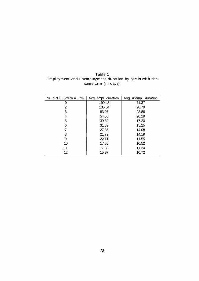
Table 1Employment and unemployment duration by spells with the

same …rm (in days)

Nr. SPELLS with = …rm: Avg. empl. duration. Avg. unempl. duration0 199.43 71.372 136.04 28.793 83.07 23.864 54.56 20.295 39.89 17.206 31.89 15.257 27.85 14.088 21.79 14.199 22.11 11.5510 17.86 10.5211 17.33 11.2412 15.97 10.72

23

Table 2Main sample characteristics for employment duration analysis

Total Sample THA workers No-THA workersTotal % Total % Total %

Total 49,322 13,614 35,708Censored 2,098 4.25 98 0.72 2,000 5.60Gender: Male 30,113 61.05 7,489 55.01 22,624 63.36Equal employer 15,759 31.95 7,177 52.72 8,582 24.03High Qual. 1,931 3.92 336 2.47 1,595 4.47Med.–High Qual. 5,074 10.29 1,012 7.43 4,062 11.38Med.–Low Qual. 17,792 36.07 5,154 37.86 12,638 35.39Low Qual. 24,525 49.72 7,112 52.24 17,413 48.76Age 16–25 16,955 34.38 5,557 40.82 11,398 31.92Age 26–35 20,085 40.72 4,747 34.87 15,338 42.95Age 36–52 12,282 24.90 3,310 24.31 8,972 25.13Duration (months)¤:1-3 26,360 55.82 9,448 69.90 16,912 50.173-6 10,822 22.92 2,419 17.90 8,403 24.936-12 5,670 12.01 960 7.10 4,710 13.9712-24 2,923 6.19 508 3.76 2,415 7.1624-36 1,197 2.53 146 1.08 1,051 3.1236-46 252 0.53 252 0.53 252 0.53Statistics¤:Average Duration 5.39 3.65 6.09Median Duration 3 2 3

*Without taking into account censored observations

24

Table 3Main sample characteristics for unemployment duration analysis

Total Sample THA workers No-THA workersTotal % Total % Total %

Total 34,137 13,033 21,104Censored 714 2.09 250 1.92 464 2.20Gender: Male 18,642 54.61 6,421 49.27 12,221 57.91Equal employer 16,994 49.78 8,432 64.70 8,562 40.57High Qual. 1,022 2.99 81 0.62 941 4.46Med.–High Qual. 2,987 8.75 751 5.76 2,236 10.60Med.–Low Qual. 12,602 36.92 5,136 39.41 7,466 35.38Low Qual. 17,526 51.34 7,065 54.21 10,461 49.57Age 16–25 16,483 48.28 7,080 54.32 9,403 44.56Age 26–35 11,102 32.52 3,673 28.18 7,429 35.20Age 36–52 6,552 19.19 2,280 17.49 4,272 20.24Duration (months)¤:1-3 23,629 70.70 10,316 80.70 13,313 64.503-6 4,640 13.88 1,396 10.92 3,244 15.726-12 3,527 10.55 738 5.77 2,789 13.5112-24 1,356 4.06 288 2.25 1,068 5.1724-30 271 0.81 45 0.35 226 1.09Statistics¤:Average Duration 3.73 2.81 4.29Median Duration 2 2 2

*Without taking into account censored observations

25

Table 4Logit Regression for Employment Hazard Rate

Without Unobs. Heter. With Unobs. Heter.Variables Coe¢cient t-statistic Coe¢cient t-statisticLog(t) -2.0714 -27.59 -2.0835 -27.63Log(t)2 1.8568 17.69 1.8682 17.75Log(t)3 -.80704 -16.36 -.81238 -16.41Log(t)4 .1100 15.23 .1111 15.31THA .5238 33.96 .53513 31.75Gender -.1130 -5.78 -.1126 -5.75Gender*Log(t) .0910 8.02 .0908 7.93High Qual. -.7432 -11.52 -.7358 -11.33High Qual.*Log(t) .1389 5.18 .1315 4.81Med.-High Qual. -.2531 -6.40 -.2476 -6.20Med.-High Qual.*Log(t) -.0250 -1.39 -.0297 -1.62Med.-Low Qual. -.0893 -4.50 -.09024 -4.48Age 26-35 -.1165 -5.67 -.1167 -5.66Age 26-35*Log(t) .0728 5.81 .0717 5.67Age 36-52 .0431 1.24 .0485 1.37Equal employer .5217 42.35 .5267 40.26Public …rm .4157 11.48 .4153 11.38Public …rm*Log(t) -.0567 -2.90 -.0544 -2.73GDP growth rate -.0982 -10.69 -.0982 -10.65GDP growth rate*Log(t) .0766 14.78 .0774 14.84Unemployment rate .0211 14.18 .0211 14.12Unempl. rate*Log(t) -.0042 -4.36 -.0039 -4.04

26

Table 4 (cont.)Logit regression for employment hazard rate

Without Unobs. Heter. With Unobs. Heter.Duration dependence Coe¢cient t-statistic Coe¢cient t-statistic

Period 6 1.7613 38.83 1.7644 38.75Period 6*GDP growth rate -0.0642 -4.49 -0.0646 -4.51Period 6*Age 26–35 -0.1528 -3.70 -0.1527 -3.69Period 6*Age 36-52 -0.2591 -5.37 -0.2602 -5.38Period 6*Public Firm -0.2423 -3.81 -0.2437 -3.82Period 12 1.5491 12.67 1.5537 12.69Period 12*GDP growth rate -0.1206 -5.37 -0.1210 -5.38Period 12*Unempl. rate 0.0154 3.02 0.0154 3.00Period 12*Age 26–35 -0.3069 -4.45 -0.3073 -4.45Period 12*Age 36–52 -0.4872 -5.55 -0.4899 -5.57Period 12*Public Firm -0.2371 -2.09 -0.2355 -2.07Period 18 1.7466 18.73 1.7482 18.73Period 18*GDP growth rate -0.1007 -3.16 -0.1009 -3.16Period 18*Age 26–35 -0.2452 -2.36 -0.3073 -4.45Period 18*Age 36–52 -0.4057 -2.93 -0.4091 -2.95Period 18*Public Firm -0.6004 -2.86 -0.5947 -2.83Period 24 1.9985 10.38 1.9916 10.32Period 24*Unempl. rate 0.0196 2.34 0.0200 2.37Period 24*Age 26–35 -0.5578 -4.92 -0.5612 -4.94Period 24*Age 36–52 -1.1895 -6.86 -1.1963 -6.88Period 24*Public Firm -0.7390 -3.27 -0.7310 -3.23Period 30 2.4294 18.97 2.4275 18.91Period 30*GDP growth rate -0.2447 -5.42 -0.2473 -5.38Period 30*Age 26–35 -0.6408 -4.13 -0.6468 -4.15Period 30*Age 36–52 -0.9256 -3.99 -0.9334 -4.01Period 30*Public Firm -0.7533 -2.19 -0.7438 -2.16Period 36 2.5423 9.85 2.5341 9.72Period 36*Unempl. rate 0.0542 4.89 0.0551 4.92Period 36*Age 26–35 -0.8963 -6.14 -0.9172 -6.21Period 36*Age 36–52 -1.1409 -5.48 -1.1613 -5.52Period 36*Public Firm -1.9360 -5.78 -1.9311 -5.74

27

Table 4 (Cont.)Logit Regression for Employment Hazard Rate

Without Unobs. Heter. With Unobs. Heter.Variables Coe¢cient t-statistic Coe¢cient t-statisticperiod 1995-1996 .6835 13.01 .6777 12.81

* Log(t) -.1532 -10.59 -.1494 -9.80* GDP growth rate -.0883 -4.66 -.0883 -4.63* High Qual. -.1154 -1.75 -.1250 -1.86* Med.- High Qual. -.1925 -4.44 -.1987 -4.49* Med.- Low Qual. -.0806 -2.90 -.0798 -2.83* Age 36-52 -.0710 -1.84 -.0796 -2.01* Public …rm .0667 1.56 .0764 1.74

period 1997-1999 .8307 12.27 .8361 12.28* Log(t) -.2813 -16.99 -.2814 -16.86* GDP growth rate -.0695 -3.66 -.0723 -3.78* High Qual. -.0905 -1.33 -.0944 -1.37* Med.- High Qual. -.2777 -6.11 -.2811 -6.10* Med.- Low Qual. -.1012 -3.44 -.1016 -3.41* Age 26-35 .0241 0.80 .0252 0.83* Age 36-52 .0703 1.64 .0654 1.50* Sex -.0778 -3.08 -.0779 -3.06* Public …rm .1772 4.17 .1828 4.23

Constant -1.3300 -31.36 -1.334 -31.11Unobserved Heterogeneity:p 0.9925 74.62´1 0.0091 0.53Log Likelihood -115,284.7 -115281.81Size 311,156 311,156

Notes: Reference category is: Female, non–THA worker, Low quali…-cation, Age 16–25, Non-equal employer, Private Employer, Fourth Quarter,Years 1990-94.

The coe¢cients for the interactions between duration dummies andother explanatory variables are not presented for space considerations.

28

Table 5Predicted Employment Average Duration for di¤erent Individual

Groups (in months)

Avg. THA no-THA 1990-94 1995-96 1997-99Full Sample 6.35 3.50 7.14 7.19 5.63 5.72MenAge 16-25Unskilled 5.43 2.51 6.32 6.06 4.62 4.80Skilled 7.87 9.80 7.44 9.15 5.71 7.32Age 26-35Unskilled 6.41 2.70 7.08 6.73 5.73 6.02Skilled 11.52 11.34 11.55 12.22 9.63 11.30Age 36-52Unskilled 5.31 2.67 6.04 6.54 5.16 5.06Skilled 11.01 9.07 11.43 12.15 9.65 11.89WomenAge 16-25Unskilled 5.39 2.90 6.27 6.34 4.63 4.01Skilled 7.52 8.64 7.18 8.34 5.05 8.36Age 26-35Unskilled 5.95 3.12 6.82 6.60 5.31 5.29Skilled 5.93 3.14 6.95 6.64 5.34 5.32Age 36-52Unskilled 4.31 2.51 5.21 6.49 4.69 3.32Skilled 8.81 8.50 8.91 9.99 8.48 8.68

29

Table 6Logit Regression for Unemployment Hazard Rate

Without Unobs. Heter. With Unobs. Heter.Variables Coe¢cient t-statistic Coe¢cient t-statisticLog(t) 2.2687 24.93 2.6735 20.78Log(t)2 -3.4392 -23.49 -3.4868 -22.37Log(t)3 1.5429 20.10 1.5234 19.04Log(t)4 -.2265 -18.05 -.2222 -17.13THA .6550 14.53 .7492 13.66THA*Log(t) -.3259 -17.40 -.3559 -16.91Gender .1062 4.723 .1256 4.84Gender*Log(t) -.0269 -1.80 -.0327 -2.06High Qual. .0381 0.937 .0491 1.08Med.-High Qual. .0145 0.481 .0158 0.47Med.-Low Qual. .1550 6.06 .1712 5.84Age 26-35 .4949 15.67 .5652 14.55Age 26-35*Log(t) -.0794 -4.58 -.0918 -4.89Age 36-52 .4581 8.27 .5213 8.12Age 36-52*Log(t) -.1558 -6.87 -.1682 -6.96Employment Duration .0153 7.08 .0174 7.04Empl. Durat*Log(t) -.0069 -4.85 -.0073 -4.84Equal Employer .8726 51.03 .9845 32.84Public …rm -.4214 -9.546 -.4969 -9.36Public …rm*Log(t) .0840 3.206 .0964 3.41Unemployment rate -.0194 -6.25 -.0210 -5.93GDP growth rate .0497 4.16 .0610 4.38GDP growth rate*Log(t) .0172 2.19 .0162 1.93

30

Table 6 (cont.)Logit Regression for Unemployment Hazard Rate

Without Unobs. Heter. With Unobs. Heter.Variables Coe¢cient t-statistic Coe¢cient t-statisticperiod 1995-1996 1.2126 12.23 1.4379 12.01

* Log(t) .1334 5.51 .1259 4.77* THA -.3907 -8.03 -.4448 -8.02* Age 26-35 -.3235 -9.02 -.3636 -8.90* Age 36-52 -.2438 -4.10 -.2740 -4.08* Med-High Qual. -.0707 -1.40 -.0705 -1.26* Med-Low Qual. -.0744 -2.19 -.0745 -1.96* Empl. Durat. -.0003 -4.33 -.0004 -4.37* GDP growth rate -.1186 -4.92 -.1584 -5.63* Unemploym. rate -.0114 -3.75 -.0130 -3.79

period 1997-1999 2.0714 18.97 2.3310 17.79* Log(t) -.2171 -8.07 -.2540 -8.42* THA -.1350 -2.64 -.1515 -2.66* Gender .1634 5.27 .1725 5.06* Age 26-35 -.5220 -12.83 -.5796 -12.54* Age 36-52 -.4356 -7.21 -.4840 -7.09* Med-Low Qual. -.0744 -2.04 -.0861 -2.12* Public Firm .1413 2.79 .1696 3.00* Equal Employer -.2485 -7.76 -.2908 -8.04* Unemploym. rate -.0215 -7.10 -.0235 -6.90* GDP growth rate -.2368 -8.31 -.2620 -8.36

Constant -1.7098 -24.41 -1.9427 -20.74Unobserved Heterogeneity:´1 1.3610 10.04p 0.2256 5.57Log Likelihood -69,211.994 -69,203.179Size 146,071 146,071

Notes: Reference category is: Female, non–THA worker,Low quali…cation, Age 16–25, Non-equal employer, Madrid, Fourth quarter

31

Table 7Predicted Unemployment Average Duration for di¤erent

Individual Groups (in months)Avg. THA no-THA 1990-94 1995-96 1997-99

Full Sample 3.08 2.72 3.21 4.97 2.31 2.06MenAge 16-25Unskilled 3.69 2.89 3.99 6.27 2.37 1.79Skilled 4.73 6.27 4.53 8.38 1.57 3.06Age 26-35Unskilled 2.51 2.13 2.64 3.02 2.13 2.21Skilled 3.12 2.96 3.14 4.24 1.94 2.46Age 36-52Unskilled 2.41 2.51 2.37 4.05 1.97 2.46Skilled 8.09 11.32 6.88 7.67 7.23 8.63WomenAge 16-25Unskilled 3.43 3.20 3.53 6.07 2.19 1.74Skilled 4.45 4.34 4.45 6.91 2.05 2.78Age 26-35Unskilled 3.21 3.07 3.26 4.17 2.88 2.79Skilled 3.29 3.35 3.27 4.17 3.01 2.38Age 36-52Unskilled 2.92 2.76 3.03 4.05 2.65 2.85Skilled 5.34 5.99 5.04 6.81 3.62 6.22

32

Table 8Estimations for the Sub-samples with Information on Type of

Contracts

Employment Hazard Unemployment HazardVariables Odds Ratio t-statistic Odds Ratio t-statisticPermanent contract .3967 -23.35 .8374 -2.26Part-time contract 1.4117 16.65 .8998 -4.35New permanent contract .4609 -7.29 1.5637 1.31Change to perm. contract .7510 -2.19 .9952 -0.01Log Likelihood -52,636.562 -31,401.992Size 148,347 62,895

Notes: Reference category is: Female, non–THA worker, Lowquali…cation, Age 16–29, Non-equal employer, Fourth quarter.

The rest of regressors are omitted for space consideration.

33

Figure 1: Kaplan-Meier Estimates of the Employment Hazard Rate

0

0,05

0,1

0,15

0,2

0,25

0,3

0,35

1 2 3 4 5 6 7 8 9 10 11 12 13 14 15 16 17 18 19 20 21 22 23 24 25 26 27 28 29 30 31 32 33 34 35 36 37 38 39 40 41 42 43 44 45 46

Figure 2: Employment Hazard Rates for THA and non-THA workers

0

0,05

0,1

0,15

0,2

0,25

0,3

0,35

0,4

0,45

1 2 3 4 5 6 7 8 9 10 11 12 13 14 15 16 17 18 19 20 21 22 23 24 25 26 27 28 29 30 31 32 33 34 35 36 37 38 39 40 41 42 43 44 45 46

THA

No-THA

34

Figure 3: Employment Hazard Rates: the e¤ect of quali…cation

0

0,05

0,1

0,15

0,2

0,25

0,3

0,35

0,4

1 2 3 4 5 6 7 8 9 10 11 12 13 14 15 16 17 18 19 20 21 22 23 24 25 26 27 28 29 30 31 32 33 34 35 36 37 38 39 40 41 42 43 44 45 46

Qual. HighQual. Med.-HighQual Med.-LowQual. Low

Figure 4: Employment Hazard Rates and the business cycle

0

0,05

0,1

0,15

0,2

0,25

0,3

0,35

0,4

0,45

1 2 3 4 5 6 7 8 9 10 11 12 13 14 15 16 17 18 19 20 21 22 23 24 25 26 27 28 29 30 31 32 33 34 35 36 37 38 39 40 41 42 43 44 45 46

Expansion

Recession

35

Figure 5: Employment Hazard Rates in three di¤erent periods

0

0,05

0,1

0,15

0,2

0,25

0,3

0,35

0,4

1 2 3 4 5 6 7 8 9 10 11 12 13 14 15 16 17 18 19 20 21 22 23 24 25 26 27 28 29 30 31 32 33 34 35 36 37 38 39 40 41 42 43 44 45 46

1990-94

1995-96

1997-99

Figure 6: Kaplan-Meier Estimates of the Unemployment Hazard Rate

0

0,05

0,1

0,15

0,2

0,25

0,3

0,35

0,4

1 2 3 4 5 6 7 8 9 10 11 12 13 14 15 16 17 18 19 20 21 22 23 24 25 26 27 28 29 30

36

Figure 7: Unemployment Hazard Rate for THA and non-THA workers

0

0,05

0,1

0,15

0,2

0,25

0,3

0,35

0,4

0,45

1 2 3 4 5 6 7 8 9 10 11 12 13 14 15 16 17 18 19 20 21 22 23 24 25 26 27 28 29 30

THA

No-THA

Figure 8: Unemployment Hazard Rate and the Business Cycle

0

0,05

0,1

0,15

0,2

0,25

0,3

0,35

0,4

0,45

1 2 3 4 5 6 7 8 9 10 11 12 13 14 15 16 17 18 19 20 21 22 23 24 25 26 27 28 29 30

ExpansionRecession

37

Figure 9: Unemployment Hazard Rate in three di¤erent periods

0

0,05

0,1

0,15

0,2

0,25

0,3

0,35

0,4

0,45

1 2 3 4 5 6 7 8 9 10 11 12 13 14 15 16 17 18 19 20 21 22 23 24 25 26 27 28 29 30

1990-19941995-19961997-1999

Figure 10: Unemployment Hazard Rates: the e¤ect of unobserved heterogeneity

0

0,1

0,2

0,3

0,4

0,5

0,6

1 2 3 4 5 6 7 8 9 10 11 12 13 14 15 16 17 18 19 20 21 22 23 24 25 26 27 28 29 30

With eta1With eta2

38