1

THE NEXUS BETWEEN ENERGY CONSUMPTION AND ECONOMIC GROWTH IN OECD COUNTRIES: A DECOMPOSITION ANALYSIS

Sahar Shafiei, Ruhul A. Salim

and Helen Cabalu

School of Economics & Finance,

Curtin Business School, Curtin University, Perth, WA 6845,

Australia

Abstract This paper analyses and compares the impacts of renewable and non-renewable energy

consumption on economic activities to find out whether economic growth benefits from

substituting renewable energy for non-renewable energy sources. Empirical results show that

both energy sources stimulate economic growth in OECD countries. However, comparing

their effects confirms that non-renewables are still the dominant source of energy utilised in

the process of economic growth. The causality analyses show that there is bidirectional

causality between economic growth and both renewable and non-renewable energy

consumption in the short- and long run. This finding confirms the feedback hypothesis which

implies that a high level of economic growth leads to high level of consumption in both

renewable and non-renewable energy and vice-versa.

Keywords: Cobb-Douglas production function; Renewable energy consumption; Non-

renewable energy consumption; Real GDP; Industrial output.

JEL classification: C23, C33, Q21, Q43, Q48

2

1. Introduction

Energy is a fundamental resource in the economy and there is a very strong link

between energy use and both the level of economic activity and economic growth.

Hence, economic growth is directly related to energy consumption and is affected by

energy availability. For instance, the industrial sector has the greatest proportion of

economic activity and consumes about one third of total energy use worldwide

(UNIDO 2010). However, it should be considered that the use of energy (especially in

the case of non-renewables) generates negative impacts such as pollutant emissions.

Therefore, countries may choose the policies that mitigate pollutant emissions such as

increasing energy efficiency via substituting in cleaner sources (i.e. renewable

energy).

Although numerous studies have dealt with the relationship between energy

consumption and economic growth, most of them focus on just aggregated energy

consumption. Recently, the literature has started paying more attention to the effect of

energy consumption on economic growth in terms of renewable and non-renewable

energy sources. However, the magnitude and the direction of the effects of renewable

and non-renewable energy consumption on economic growth have not been

established and they are still unclear. Therefore, this study aims to investigate both

renewable and non-renewable energy consumption in OECD countries in order to find

whether economic growth benefits from substituting renewable energy for non-

renewable energy sources. Furthermore, the effects of disaggregated energy

consumption on the industrial sector, which has an important role in the economic

growth of countries, are also investigated. The empirical findings are based on data

for selected OECD countries over the period 1980 to 2011.

The remainder of the paper is organized as follows: Section 2 presents a review of the

existing literature. Methodology is described in Section 3, followed by the empirical

3

results in Section 4. Finally, conclusion and policy implications are provided in

Section 5.

2. Review of the Existing Literature

Recently, a new line of standard research focuses on the link between renewable

energy consumption and economic growth. Several studies find a bidirectional

relationship between renewable energy consumption and economic growth (Apergis

and Payne 2010d, Apergis and Payne 2010e, Apergis and Payne 2011b. In the case of

China for the period 1978 to 2008, Fang (2011) finds that a 1% increase in renewable

energy consumption increases real GDP by 0.12%. For 16 emerging market

economies over the period 1990 to 2007, Apergis and Payne (2011c) find a

unidirectional causality from economic growth to renewable electricity consumption

in the short run and bidirectional causality in the long run. Apergis and Payne state

that in higher levels of economic growth, more renewable energy sources will become

available. Therefore, the interdependent relationship between economic growth and

renewable energy in the long run is as expected. In addition, the results indicate that

there is bidirectional causality between non-renewable electricity consumption and

economic growth in both the short run and long run. For European and Eurasian

countries, Tiwari (2011) reveals that while the growth rate of non-renewable energy

consumption has a negative impact, the growth rate of renewable energy consumption

has a positive impact on the growth rate of GDP. Apergis and Payne (2012a) find a

unidirectional causality from renewable electricity consumption to economic growth

in the short run, but bidirectional causality in the long run in six Central American

countries. The results also indicate bidirectional causality between non-renewable

electricity consumption and economic growth in both the short run and long run.

Apergis and Payne (2012b) find bidirectional causality between renewable and non-

4

renewable energy consumption measures and economic growth in both short run and

long run for 80 developed and developing countries. Tugcu et al. (2012) assess the

long-run and causal relationships between renewable and non-renewable energy

consumption and economic growth. The results, estimated under a classical

production function, demonstrate that there is bidirectional causality between non-

renewable energy and growth in all G7 countries.

The research on the effects of fossil fuels and other energy sources on countries’

economies is limited. Moreover, a general conclusion from the studies reviewed in

this section is that there is no consensus either on the existence or on the direction of

causality between energy consumption and economic growth in the literature.

Therefore, the present study aims to contribute to the literature by identifying the

impacts of renewable and non-renewable sources of energy on the real gross domestic

product and also on the industrial sector in OECD countries. Unlike previous work,

this paper takes into account some important diagnostic tests including cross-

sectional dependency, heterogeneity, and serial correlation, to prevent misleading

inference and inconsistent estimates in the models. Furthermore, a panel stationarity

hypothesis allowing for structural breaks is tested, something that has generally

ignored previously

3. Methodology

3.1 Theoretical Framework

This section explores the theoretical and conceptual aspects of relevance to the

relationship between disaggregated energy consumption and economic growth under

the framework of Cobb-Douglas production function.

The current understanding of economic growth is largely based on the neoclassical

growth model developed by Solow (1956). The neo-classical economic models do not

include energy as a factor of production and they consider the economy as a closed

5

system within which goods are produced by inputs of capital and labour. However,

the role of energy as an important factor of production has received increasing

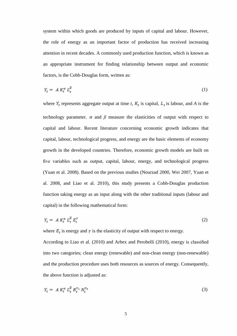
attention in recent decades. A commonly used production function, which is known as

an appropriate instrument for finding relationship between output and economic

factors, is the Cobb-Douglas form, written as:

(1)

where represents aggregate output at time t, is capital, is labour, and A is the

technology parameter. and β measure the elasticities of output with respect to

capital and labour. Recent literature concerning economic growth indicates that

capital, labour, technological progress, and energy are the basic elements of economy

growth in the developed countries. Therefore, economic growth models are built on

five variables such as output, capital, labour, energy, and technological progress

(Yuan et al. 2008). Based on the previous studies (Nourzad 2000, Wei 2007, Yuan et

al. 2008, and Liao et al. 2010), this study presents a Cobb-Douglas production

function taking energy as an input along with the other traditional inputs (labour and

capital) in the following mathematical form:

(2)

where is energy and is the elasticity of output with respect to energy.

According to Liao et al. (2010) and Arbex and Perobelli (2010), energy is classified

into two categories; clean energy (renewable) and non-clean energy (non-renewable)

and the production procedure uses both resources as sources of energy. Consequently,

the above function is adjusted as:

(3)

6

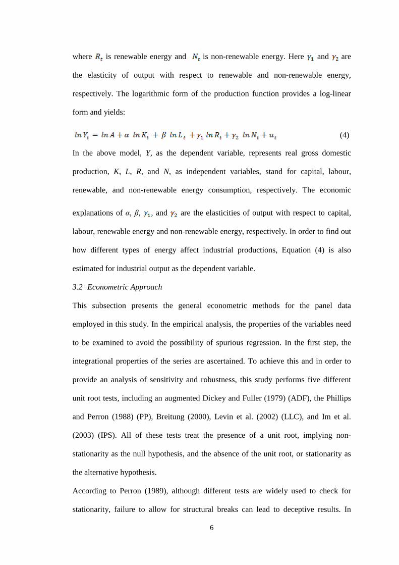
where is renewable energy and is non-renewable energy. Here and are

the elasticity of output with respect to renewable and non-renewable energy,

respectively. The logarithmic form of the production function provides a log-linear

form and yields:

(4)

In the above model, Y, as the dependent variable, represents real gross domestic

production, K, L, R, and N, as independent variables, stand for capital, labour,

renewable, and non-renewable energy consumption, respectively. The economic

explanations of α, β, , and are the elasticities of output with respect to capital,

labour, renewable energy and non-renewable energy, respectively. In order to find out

how different types of energy affect industrial productions, Equation (4) is also

estimated for industrial output as the dependent variable.

3.2 Econometric Approach

This subsection presents the general econometric methods for the panel data

employed in this study. In the empirical analysis, the properties of the variables need

to be examined to avoid the possibility of spurious regression. In the first step, the

integrational properties of the series are ascertained. To achieve this and in order to

provide an analysis of sensitivity and robustness, this study performs five different

unit root tests, including an augmented Dickey and Fuller (1979) (ADF), the Phillips

and Perron (1988) (PP), Breitung (2000), Levin et al. (2002) (LLC), and Im et al.

(2003) (IPS). All of these tests treat the presence of a unit root, implying non-

stationarity as the null hypothesis, and the absence of the unit root, or stationarity as

the alternative hypothesis.

According to Perron (1989), although different tests are widely used to check for

stationarity, failure to allow for structural breaks can lead to deceptive results. In

7

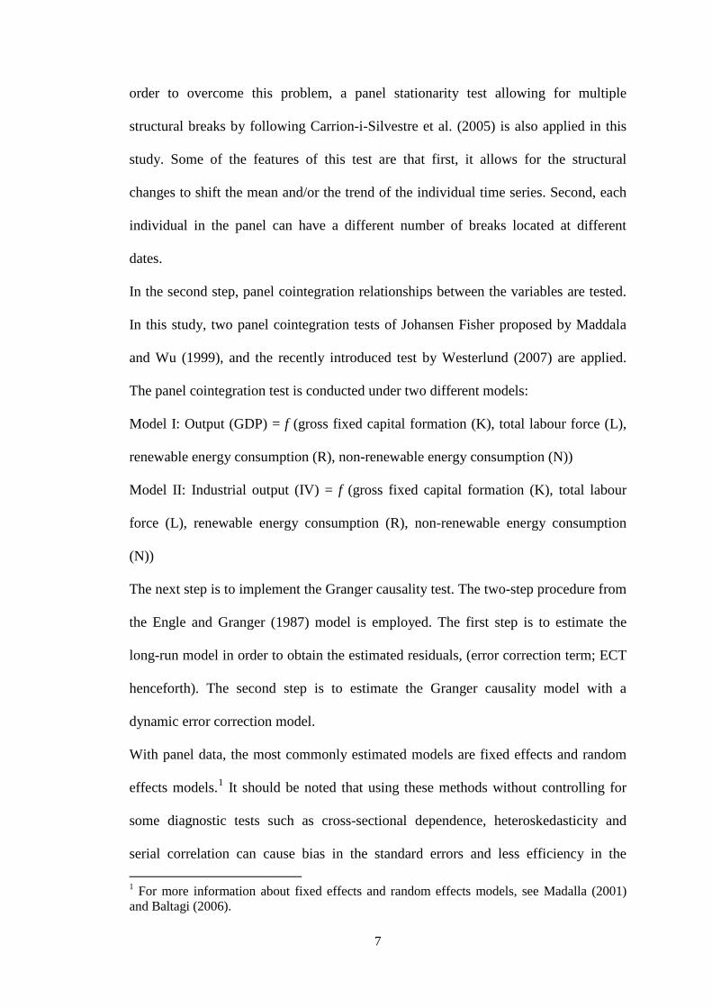
order to overcome this problem, a panel stationarity test allowing for multiple

structural breaks by following Carrion-i-Silvestre et al. (2005) is also applied in this

study. Some of the features of this test are that first, it allows for the structural

changes to shift the mean and/or the trend of the individual time series. Second, each

individual in the panel can have a different number of breaks located at different

dates.

In the second step, panel cointegration relationships between the variables are tested.

In this study, two panel cointegration tests of Johansen Fisher proposed by Maddala

and Wu (1999), and the recently introduced test by Westerlund (2007) are applied.

The panel cointegration test is conducted under two different models:

Model I: Output (GDP) = f (gross fixed capital formation (K), total labour force (L),

renewable energy consumption (R), non-renewable energy consumption (N))

Model II: Industrial output (IV) = f (gross fixed capital formation (K), total labour

force (L), renewable energy consumption (R), non-renewable energy consumption

(N))

The next step is to implement the Granger causality test. The two-step procedure from

the Engle and Granger (1987) model is employed. The first step is to estimate the

long-run model in order to obtain the estimated residuals, (error correction term; ECT

henceforth). The second step is to estimate the Granger causality model with a

dynamic error correction model.

With panel data, the most commonly estimated models are fixed effects and random

effects models.1 It should be noted that using these methods without controlling for

some diagnostic tests such as cross-sectional dependence, heteroskedasticity and

serial correlation can cause bias in the standard errors and less efficiency in the 1 For more information about fixed effects and random effects models, see Madalla (2001) and Baltagi (2006).

8

results. Therefore, it can be said that choosing an appropriate estimation method also

depends on identifying the diagnostic tests in a panel data model. In the present study,

three tests including Friedman (1937), Frees (1995), and Pesaran (2004) are applied to

check for cross-section dependence.

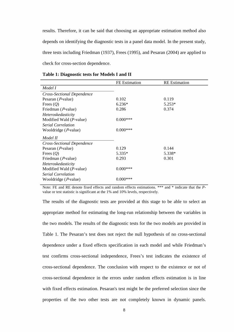
Table 1: Diagnostic tests for Models I and II

FE Estimation RE Estimation Model I Cross-Sectional Dependence Pesaran (P-value) 0.102 0.119 Frees (Q) 6.236* 5.253* Friedman (P-value) 0.286 0.374 Heteroskedasticity Modified Wald (P-value) 0.000*** Serial Correlation Wooldridge (P-value) 0.000*** Model II Cross-Sectional Dependence Pesaran (P-value) 0.129 0.144 Frees (Q) 5.335* 5.338* Friedman (P-value) 0.293 0.301 Heteroskedasticity Modified Wald (P-value) 0.000*** Serial Correlation Wooldridge (P-value) 0.000*** Note: FE and RE denote fixed effects and random effects estimations. *** and * indicate that the P-value or test statistic is significant at the 1% and 10% levels, respectively.

The results of the diagnostic tests are provided at this stage to be able to select an

appropriate method for estimating the long-run relationship between the variables in

the two models. The results of the diagnostic tests for the two models are provided in

Table 1. The Pesaran’s test does not reject the null hypothesis of no cross-sectional

dependence under a fixed effects specification in each model and while Friedman’s

test confirms cross-sectional independence, Frees’s test indicates the existence of

cross-sectional dependence. The conclusion with respect to the existence or not of

cross-sectional dependence in the errors under random effects estimation is in line

with fixed effects estimation. Pesaran's test might be the preferred selection since the

properties of the two other tests are not completely known in dynamic panels.

9

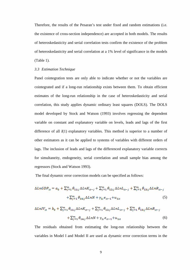
Therefore, the results of the Pesaran’s test under fixed and random estimations (i.e.

the existence of cross-section independence) are accepted in both models. The results

of heteroskedasticity and serial correlation tests confirm the existence of the problem

of heteroskedasticity and serial correlation at a 1% level of significance in the models

(Table 1).

3.3 Estimation Technique

Panel cointegration tests are only able to indicate whether or not the variables are

cointegrated and if a long-run relationship exists between them. To obtain efficient

estimates of the long-run relationship in the case of heteroskedasticity and serial

correlation, this study applies dynamic ordinary least squares (DOLS). The DOLS

model developed by Stock and Watson (1993) involves regressing the dependent

variable on constant and explanatory variable on levels, leads and lags of the first

difference of all I(1) explanatory variables. This method is superior to a number of

other estimators as it can be applied to systems of variables with different orders of

lags. The inclusion of leads and lags of the differenced explanatory variable corrects

for simultaneity, endogeneity, serial correlation and small sample bias among the

regressors (Stock and Watson 1993).

The final dynamic error correction models can be specified as follows:

(5)

(6)

The residuals obtained from estimating the long-run relationship between the

variables in Model I and Model II are used as dynamic error correction terms in the

10

above equations. The causal relationship between the variables is tested considering

each variable in turn as a dependent variable in each equation.

Because is correlated with the first difference error term, (= − )

(Equation 3.10), it is necessary to use instrumental variable procedures to cope with

this problem. A possible solution is represented by the Generalised Method of

Moments (GMM) technique. Therefore, this study employs a GMM dynamic panel

model to estimate the Equations (5) and (6). In the system GMM estimator, lagged

differences of the series are used as instruments for the equations. They are derived

from the estimation of a system of two simultaneous equations, one in levels (with

lagged first differences as instruments) and the other in first differences (with lagged

levels as instruments). This study uses the system GMM estimator which seems to

have superior finite sample properties.

3.4 Data Description

Annual data for a set of 29 OECD countries covering the period from 1980 to 2011

are collected on gross domestic product, industrial output, capital, labour force,

renewable energy consumption and non-renewable energy consumption for a

balanced panel with 928 observations for the selected OECD countries.2

In this study, real GDP in billions of constant 2000 U.S. dollars using purchasing

power parities (PPPs) are used as a proxy for economic output. Capital, which is used

as an input in the production function in fact refers to already-produced durable

goods. Since capital stock data are not easy to collect and measure, gross fixed capital

formation is usually used as a proxy for growth of capital stock. Particularly, in

accordance with the perpetual inventory method assuming a constant depreciation rate 2 The 29 sample countries are Australia, Austria, Belgium, Canada, Chile, Denmark, Finland, France, Germany, Greece, Hungary, Iceland, Ireland, Italy, Japan, South Korea, Luxembourg, Mexico, the Netherlands, New Zealand, Norway, Poland, Portugal, Spain, Sweden, Switzerland, Turkey, the United Kingdom and the United States.

11

indicates that changes in investment closely follow changes in the capital stock3.

Thus, data of real gross fixed capital formation in billions of constant 2000 U.S.

dollars are used in this study. Data on total labour force in millions, as well as

industrial value added (as a proxy for industrial output) in billions of constant 2000

U.S. dollars are also applied. All the data mentioned above are obtained from the

World Bank (2012).

According to the Energy Information Administration, non-renewable energy sources

include coal and coal products, oil, and natural gas. Therefore, in this study, non-

renewable energy consumption is measured as the aggregate of the consumption of all

these sources in quadrillion Btu units. Renewable energy consumption in quadrillion

Btu units is measured as wood, waste, geothermal, wind, photovoltaic, and solar

thermal energy consumption. All the data related to energy consumption are sourced

from the U.S. Energy Information Administration.

All the variables are converted into natural logarithms prior to conducting the

analysis, so that the parameter estimates of the model can be interpreted as elasticity

estimates.4

4. Empirical Results

4.1 Panel Unit Root Test

The results of the unit root tests, including augmented Dickey and Fuller (1979)

(ADF), the Phillips and Perron (1988) (PP), Breitung (2000), Levin et al. (2002)

(LLC), and Im et al. (2003) (IPS) are presented in Table 3. All of these tests treat the

presence of a unit root, implying non stationarity as the null hypothesis, and the

3 See Soytas and Sari (2006), 742. 4 To test for multicollinearity between the independent variables in each model, the variance inflation factors (VIF) for each predictor is calculated. The results indicate no existence of multicollinearity between the independent variables in each of the models.

12

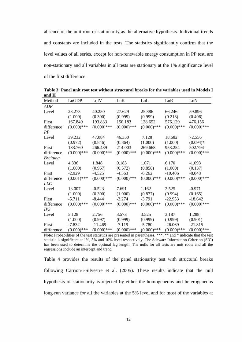
absence of the unit root or stationarity as the alternative hypothesis. Individual trends

and constants are included in the tests. The statistics significantly confirm that the

level values of all series, except for non-renewable energy consumption in PP test, are

non-stationary and all variables in all tests are stationary at the 1% significance level

of the first difference.

Table 3: Panel unit root test without structural breaks for the variables used in Models I and II Method LnGDP LnIV LnK LnL LnR LnN ADF Level 23.273

(1.000) 40.250 (0.300)

27.629 (0.999)

25.886 (0.999)

66.246 (0.213)

59.896 (0.406)

First difference

167.840 (0.000)***

193.833 (0.000)***

150.183 (0.000)***

128.652 (0.000)***

576.129 (0.000)***

476.156 (0.000)***

PP Level 39.232

(0.972) 47.084 (0.846)

46.350 (0.864)

7.128 (1.000)

18.682 (1.000)

72.556 (0.094)*

First difference

183.760 (0.000)***

266.439 (0.000)***

214.003 (0.000)***

269.668 (0.000)***

953.254 (0.000)***

502.794 (0.000)***

Breitung Level 4.336

(1.000) 1.848 (0.967)

0.183 (0.572)

1.071 (0.858)

6.170 (1.000)

-1.093 (0.137)

First difference

-2.929 (0.001)***

-4.525 (0.000)***

-4.563 (0.000)***

-6.262 (0.000)***

-10.406 (0.000)***

-8.048 (0.000)***

LLC Level 13.007

(1.000) -0.523 (0.300)

7.691 (1.000)

1.162 (0.877)

2.525 (0.994)

-0.971 (0.165)

First difference

-5.711 (0.000)***

-8.444 (0.000)***

-3.274 (0.000)***

-3.791 (0.000)***

-22.953 (0.000)***

-18.642 (0.000)***

IPS Level 5.128

(1.000) 2.756 (0.997)

3.573 (0.999)

3.525 (0.999)

3.187 (0.999)

1.288 (0.901)

First difference

-7.832 (0.000)***

-11.469 (0.000)***

-7.119 (0.000)***

-5.780 (0.000)***

-26.069 (0.000)***

-21.815 (0.000)***

Note: Probabilities of the test statistics are presented in parentheses. ***, ** and * indicate that the test statistic is significant at 1%, 5% and 10% level respectively. The Schwarz Information Criterion (SIC) has been used to determine the optimal lag length. The nulls for all tests are unit roots and all the regressions include an intercept and trend.

Table 4 provides the results of the panel stationarity test with structural breaks

following Carrion-i-Silvestre et al. (2005). These results indicate that the null

hypothesis of stationarity is rejected by either the homogeneous and heterogeneous

long-run variance for all the variables at the 5% level and for most of the variables at

13

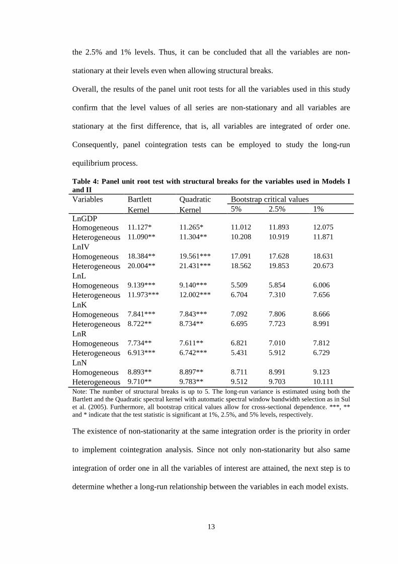
the 2.5% and 1% levels. Thus, it can be concluded that all the variables are non-

stationary at their levels even when allowing structural breaks.

Overall, the results of the panel unit root tests for all the variables used in this study

confirm that the level values of all series are non-stationary and all variables are

stationary at the first difference, that is, all variables are integrated of order one.

Consequently, panel cointegration tests can be employed to study the long-run

equilibrium process.

Table 4: Panel unit root test with structural breaks for the variables used in Models I and II Variables Bartlett

Kernel Quadratic Kernel

Bootstrap critical values 5% 2.5% 1%

LnGDP Homogeneous 11.127* 11.265* 11.012 11.893 12.075 Heterogeneous

11.090** 11.304** 10.208 10.919 11.871 LnIV Homogeneous 18.384** 19.561*** 17.091 17.628 18.631 Heterogeneous 20.004** 21.431*** 18.562 19.853 20.673 LnL Homogeneous 9.139*** 9.140*** 5.509 5.854 6.006 Heterogeneous

11.973*** 12.002*** 6.704 7.310 7.656 LnK Homogeneous 7.841*** 7.843*** 7.092 7.806 8.666 Heterogeneous

8.722** 8.734** 6.695 7.723 8.991 LnR Homogeneous 7.734** 7.611** 6.821 7.010 7.812 Heterogeneous

6.913*** 6.742*** 5.431 5.912 6.729 LnN Homogeneous 8.893** 8.897** 8.711 8.991 9.123 Heterogeneous 9.710** 9.783** 9.512 9.703 10.111 Note: The number of structural breaks is up to 5. The long-run variance is estimated using both the Bartlett and the Quadratic spectral kernel with automatic spectral window bandwidth selection as in Sul et al. (2005). Furthermore, all bootstrap critical values allow for cross-sectional dependence. ***, ** and * indicate that the test statistic is significant at 1%, 2.5%, and 5% levels, respectively.

The existence of non-stationarity at the same integration order is the priority in order

to implement cointegration analysis. Since not only non-stationarity but also same

integration of order one in all the variables of interest are attained, the next step is to

determine whether a long-run relationship between the variables in each model exists.

14

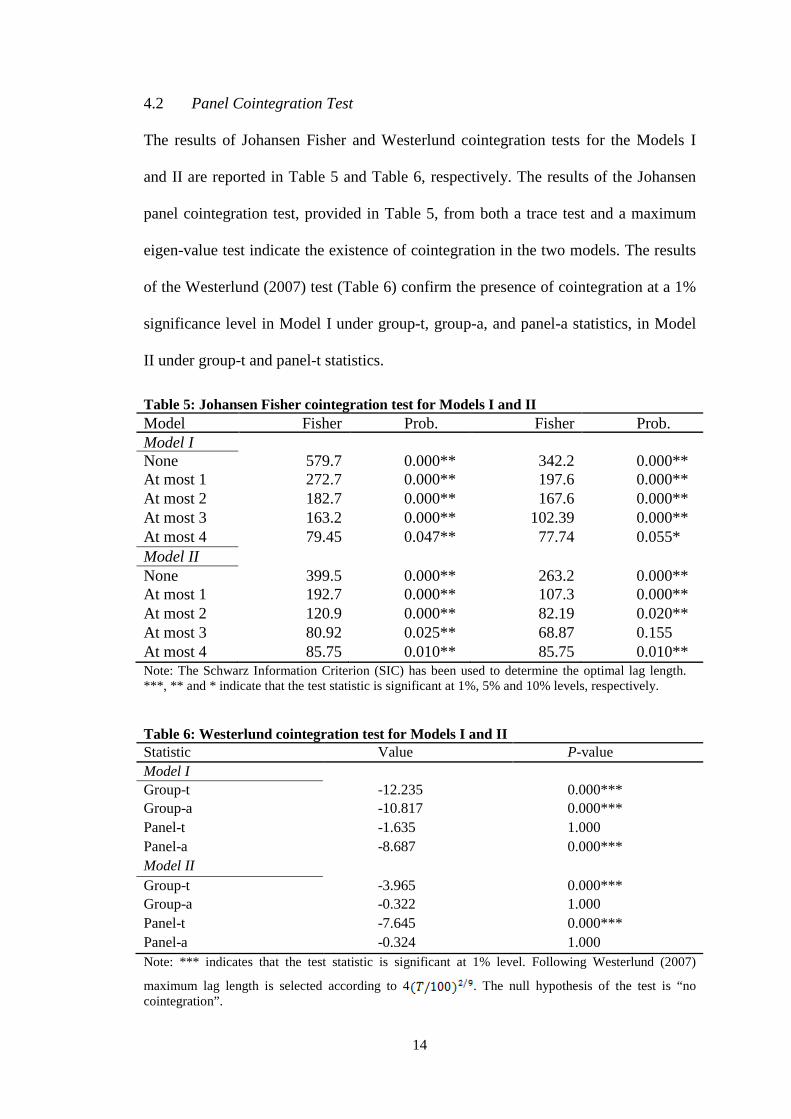
4.2 Panel Cointegration Test

The results of Johansen Fisher and Westerlund cointegration tests for the Models I

and II are reported in Table 5 and Table 6, respectively. The results of the Johansen

panel cointegration test, provided in Table 5, from both a trace test and a maximum

eigen-value test indicate the existence of cointegration in the two models. The results

of the Westerlund (2007) test (Table 6) confirm the presence of cointegration at a 1%

significance level in Model I under group-t, group-a, and panel-a statistics, in Model

II under group-t and panel-t statistics.

Table 5: Johansen Fisher cointegration test for Models I and II Model Fisher

Prob. Fisher

Prob. Model I None 579.7 0.000**

342.2 0.000**

At most 1

272.7 0.000**

197.6 0.000**

At most 2 182.7 0.000**

167.6 0.000**

At most 3 163.2 0.000**

102.39 0.000**

At most 4 79.45 0.047** 77.74 0.055* Model II None 399.5 0.000**

263.2 0.000**

At most 1 192.7 0.000**

107.3 0.000**

At most 2 120.9 0.000**

82.19 0.020**

At most 3 80.92 0.025** 68.87 0.155 At most 4 85.75 0.010** 85.75 0.010** Note: The Schwarz Information Criterion (SIC) has been used to determine the optimal lag length. ***, ** and * indicate that the test statistic is significant at 1%, 5% and 10% levels, respectively.

Table 6: Westerlund cointegration test for Models I and II Statistic Value P-value Model I Group-t -12.235 0.000*** Group-a -10.817 0.000*** Panel-t -1.635 1.000 Panel-a -8.687 0.000*** Model II Group-t -3.965 0.000*** Group-a -0.322 1.000 Panel-t -7.645 0.000*** Panel-a -0.324 1.000 Note: *** indicates that the test statistic is significant at 1% level. Following Westerlund (2007)

maximum lag length is selected according to 4 . The null hypothesis of the test is “no cointegration”.

15

To summarize, it is clearly seen that the results of the Johansen Fisher and Westerlund

tests for cointegration are consistent, implying that a long-run equilibrium relationship

exists between GDP, capital, labour force, renewable and non-renewable energy

consumption in selected OECD countries.

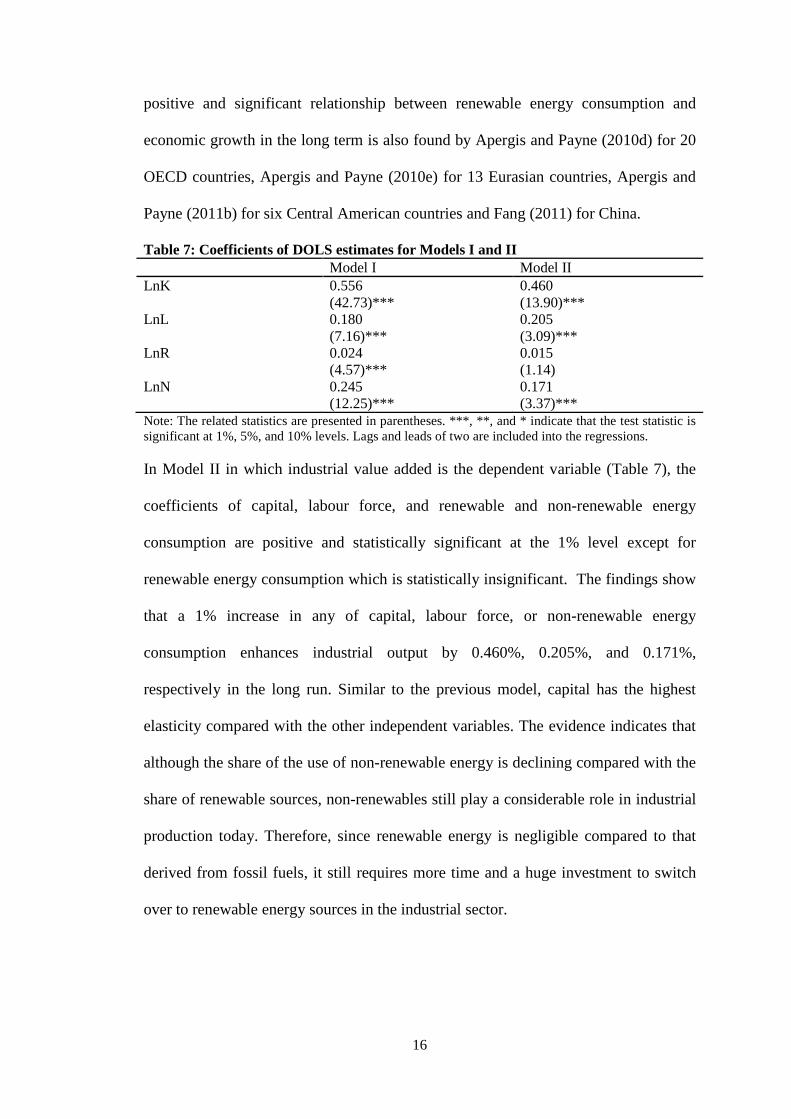
4.3 Long-Run Estimation

Table 7 presents the results of estimating the long-run relationship between the

variables in the four Models I and II based on the DOLS method. For real gross

domestic product (Model I), the coefficients of real gross fixed capital formation

(capital), total labour force, renewable, and non-renewable energy consumption are

positive and significant at the 1% level. These results show that in the long run a 1%

increase in capital, total labour force, renewable, and non-renewable energy

consumption will enhance real GDP by 0.556%, 0.180%, 0.024%, and 0.245%,

respectively. Comparing the coefficients of the independent variables indicates that

capital has the largest effect on real GDP in the long run. In addition, the elasticities

of real GDP with respect to renewable and non-renewable energy consumption

demonstrate that both types of energy stimulate economic growth in OECD countries.

However, comparing the magnitudes of their coefficients confirms that non-

renewables are still the dominant type of energy utilized in the process of economic

growth. Comparison with other studies in which the effects of renewable and non-

renewable energy consumption are simultaneously investigated on economic growth

show that the results obtained here are consistent with those reported by Apergis and

Payne (2012b) for 80 developed and developing countries. However, the results are

different from those by Apergis and Payne (2011c) and Apergis and Payne (2012a)

who find positive and significant impact only for non-renewable energy consumption

in 16 emerging countries and in six Central American countries, respectively. Finding

16

positive and significant relationship between renewable energy consumption and

economic growth in the long term is also found by Apergis and Payne (2010d) for 20

OECD countries, Apergis and Payne (2010e) for 13 Eurasian countries, Apergis and

Payne (2011b) for six Central American countries and Fang (2011) for China.

Table 7: Coefficients of DOLS estimates for Models I and II Model I Model II LnK 0.556 0.460 (42.73)*** (13.90)*** LnL 0.180 0.205 (7.16)*** (3.09)*** LnR 0.024 0.015 (4.57)*** (1.14) LnN 0.245 0.171 (12.25)*** (3.37)*** Note: The related statistics are presented in parentheses. ***, **, and * indicate that the test statistic is significant at 1%, 5%, and 10% levels. Lags and leads of two are included into the regressions.

In Model II in which industrial value added is the dependent variable (Table 7), the

coefficients of capital, labour force, and renewable and non-renewable energy

consumption are positive and statistically significant at the 1% level except for

renewable energy consumption which is statistically insignificant. The findings show

that a 1% increase in any of capital, labour force, or non-renewable energy

consumption enhances industrial output by 0.460%, 0.205%, and 0.171%,

respectively in the long run. Similar to the previous model, capital has the highest

elasticity compared with the other independent variables. The evidence indicates that

although the share of the use of non-renewable energy is declining compared with the

share of renewable sources, non-renewables still play a considerable role in industrial

production today. Therefore, since renewable energy is negligible compared to that

derived from fossil fuels, it still requires more time and a huge investment to switch

over to renewable energy sources in the industrial sector.

17

4.4 Panel Granger Causality

The results of the short-run and long-run Granger causality tests for Model I and

Model II are presented in this section. Beginning with Model I, the results reported in

Table 8 show that real gross fixed capital formation, total labour force, renewable and

non-renewable energy consumption each has a positive and significant effect on real

GDP. The coefficients of all the variables are significant at the 1% level except for

total labour force which is significant at the 5% level. This suggests that real gross

fixed capital formation, total labour force, renewable and non-renewable energy

consumption do Granger cause economic growth in the short run. In estimating the

second equation in which real gross fixed capital formation is the dependent variable,

the impacts of real GDP, total labour force on the real gross fixed capital formation

are positive and statistically significant at the 1% and 5% level, respectively. In

addition, the effects of renewable and non-renewable energy consumption on the real

gross fixed capital formation are also positive and significant at the 1% level. This

shows that economic growth, total labour force, renewable and non-renewable energy

consumption cause the real gross fixed capital formation in the short run. In regards to

the third equation, only real gross fixed capital formation has a positive and

significant impact at the 5% level on the total labour force. This result indicates that

real gross fixed capital formation is the only factor that Granger cause total labour

force in the short run.

With respect to the fourth equation for renewable energy consumption, real GDP and

real gross fixed capital formation each has a positive and statistically significant effect

at the 1% level on renewable energy consumption. This demonstrates that real GDP

and real gross fixed capital formation Granger cause renewable energy consumption

in the short run. Finally, for the last equation, real GDP, real gross fixed capital

18

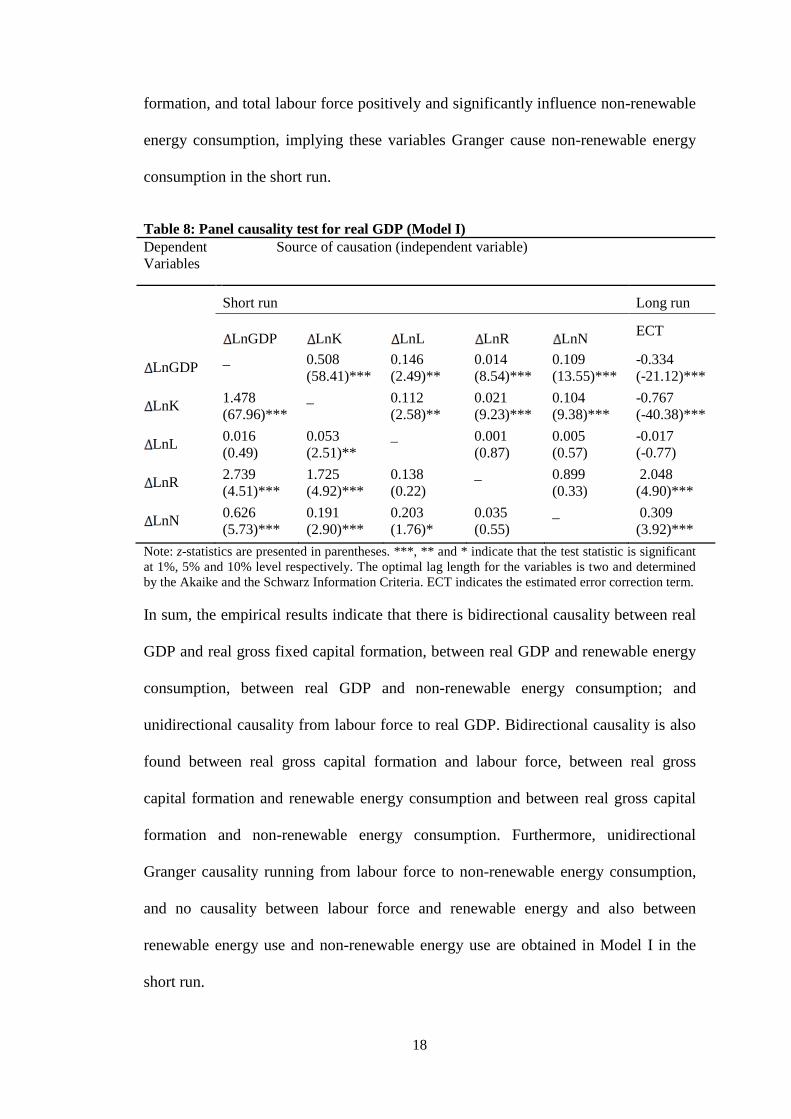
formation, and total labour force positively and significantly influence non-renewable

energy consumption, implying these variables Granger cause non-renewable energy

consumption in the short run.

Table 8: Panel causality test for real GDP (Model I) Dependent Variables

Source of causation (independent variable)

Short run Long run

LnGDP LnK LnL LnR LnN ECT

LnGDP _ 0.508 (58.41)***

0.146 (2.49)**

0.014 (8.54)***

0.109 (13.55)***

-0.334 (-21.12)***

LnK 1.478 (67.96)***

_ 0.112 (2.58)**

0.021 (9.23)***

0.104 (9.38)***

-0.767 (-40.38)***

LnL 0.016 (0.49)

0.053 (2.51)**

_ 0.001 (0.87)

0.005 (0.57)

-0.017 (-0.77)

LnR 2.739 (4.51)***

1.725 (4.92)***

0.138 (0.22)

_ 0.899 (0.33)

2.048 (4.90)***

LnN 0.626 (5.73)***

0.191 (2.90)***

0.203 (1.76)*

0.035 (0.55)

_ 0.309 (3.92)***

Note: z-statistics are presented in parentheses. ***, ** and * indicate that the test statistic is significant at 1%, 5% and 10% level respectively. The optimal lag length for the variables is two and determined by the Akaike and the Schwarz Information Criteria. ECT indicates the estimated error correction term.

In sum, the empirical results indicate that there is bidirectional causality between real

GDP and real gross fixed capital formation, between real GDP and renewable energy

consumption, between real GDP and non-renewable energy consumption; and

unidirectional causality from labour force to real GDP. Bidirectional causality is also

found between real gross capital formation and labour force, between real gross

capital formation and renewable energy consumption and between real gross capital

formation and non-renewable energy consumption. Furthermore, unidirectional

Granger causality running from labour force to non-renewable energy consumption,

and no causality between labour force and renewable energy and also between

renewable energy use and non-renewable energy use are obtained in Model I in the

short run.

19

The results of bidirectional causality between real GDP and renewable energy

consumption as well as between real GDP and non-renewable energy consumption

are consistent with Apergis and Payne (2012b) who also investigate the two types of

energy simultaneously for 80 developed and developing countries. The results on the

relationship between real GDP and non-renewable energy consumption is also similar

to the finding of Apergis and Payne (2011c) for 16 emerging economies and Apergis

and Payne (2012a) for six Central American countries. However, the results with

respect to the relationship between economic growth and renewable energy use are

different with those (Apergis and Payne 2011c; Apergis and Payne 2012a) who find

unidirectional causality from GDP to renewable energy use and unidirectional

causality from renewable energy use to GDP, respectively.

Focusing on the causality between economic growth and renewable energy

consumption, the result obtained in this study is consistent with Apergis and Payne

(2010d) for 20 OECD countries, Apergis and Payne (2010e) for Eurasia countries and

Apergis and Payne (2011b) for Central American countries. The finding of

bidirectional causality between economic growth and the two types of energy

confirms the feedback hypothesis implying that a high level of economic growth leads

to high level of consumption in both renewable and non-renewable energy and vice-

versa. However, the governments should substitute renewable energy sources for non-

renewable energy sources and encourage more usage of renewables in order to

mitigate pollutant emissions.

The long-run dynamics displayed by the error correction terms in Model I confirm

evidence of the presence of bidirectional causality between renewable energy

consumption and real GDP as well as between non-renewable energy consumption

and real GDP. In addition, the coefficient of the error correction term in the first

20

equation suggests that the deviation of real GDP from short run to the long run is

corrected by 33% each year; and convergence to equilibrium after a shock to real

GDP takes about 3 years5 (Table 8).

Turning to Model II (Table 9), the results of Granger causality between the variables

in the first equation indicate that real gross capital formation and renewable energy

consumption have a positive and statistically significant effect at the 1% level and

labour force and non-renewable energy consumption have a positive and significant

effect at the 5% level on industrial output. The findings suggest that capital, labour

force, and both renewable and non-renewable energy consumption do Granger cause

industrial output in the short run. Considering the causality relationship between

industrial output and the other variables in rest of the equations, the results show that

industrial output positively and significantly influences gross capital formation, labour

force, and both renewable and non-renewable energy consumption. This suggests that

industrial output Granger cause capital, labour force, and both renewable and non-

renewable energy use in the short run.

Overall, the results of Model II (Table 9) indicate that there is bidirectional causality

between industrial output and each of capital, labour force, renewable and non-

renewable energy consumption. The two-way relationship between industrial output

and both kinds of energy which supports a feedback hypothesis implies that

renewable and non-renewable energy consumption mutually influences each other in

OECD countries in the short run. Therefore, energy conservation in terms of either

renewable or non-renewable may lead to a reduction in industrial production. On the

other hand, any negative shock in the process of industrial output can have a negative

impact on energy.

5 The number of years is calculated as the inverse of the absolute value of the ECT.

21

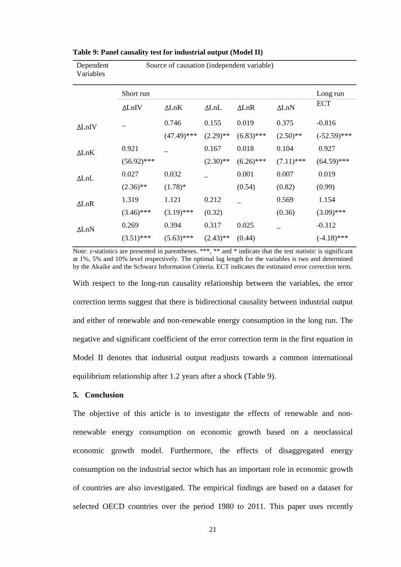
Table 9: Panel causality test for industrial output (Model II)

Dependent Variables

Source of causation (independent variable)

Short run Long run

LnIV LnK LnL LnR LnN ECT

LnIV _ 0.746

(47.49)***

0.155

(2.29)**

0.019

(6.83)***

0.375

(2.50)**

-0.816

(-52.59)***

LnK 0.921

(56.92)***

_ 0.167

(2.30)**

0.018

(6.26)***

0.104

(7.11)***

0.927

(64.59)***

LnL 0.027

(2.36)**

0.032

(1.78)*

_ 0.001

(0.54)

0.007

(0.82)

0.019

(0.99)

LnR 1.319

(3.46)***

1.121

(3.19)***

0.212

(0.32)

_ 0.569

(0.36)

1.154

(3.09)***

LnN 0.269

(3.51)***

0.394

(5.63)***

0.317

(2.43)**

0.025

(0.44)

_ -0.312

(-4.18)***

Note: z-statistics are presented in parentheses. ***, ** and * indicate that the test statistic is significant at 1%, 5% and 10% level respectively. The optimal lag length for the variables is two and determined by the Akaike and the Schwarz Information Criteria. ECT indicates the estimated error correction term.

With respect to the long-run causality relationship between the variables, the error

correction terms suggest that there is bidirectional causality between industrial output

and either of renewable and non-renewable energy consumption in the long run. The

negative and significant coefficient of the error correction term in the first equation in

Model II denotes that industrial output readjusts towards a common international

equilibrium relationship after 1.2 years after a shock (Table 9).

5. Conclusion

The objective of this article is to investigate the effects of renewable and non-

renewable energy consumption on economic growth based on a neoclassical

economic growth model. Furthermore, the effects of disaggregated energy

consumption on the industrial sector which has an important role in economic growth

of countries are also investigated. The empirical findings are based on a dataset for

selected OECD countries over the period 1980 to 2011. This paper uses recently

22

developed panel unit root and panel cointegration tests and also applies a more

recently used method, Dynamic OLS (DOLS) in order to estimate the long-run

relationship between the variables. The results of cointegration tests indicate the

existence of a long-run equilibrium relationship between the variables. With respect to

the long-run estimation, for real gross domestic product (Model I), the coefficients of

real gross fixed capital formation (capital), total labour force, renewable, and non-

renewable energy consumption are positive and significant at 1% level. The

elasticities of real GDP with respect to renewable and non-renewable energy

consumption demonstrate that both types of energy stimulate economic growth in

OECD countries. However, comparing the magnitudes of their coefficients confirms

that non-renewables are still the dominant type of energy utilised in the process of

economic growth. Similar results are obtained for industrial output, indicating that

although the share of the use of non-renewable energy is declining compared with the

share of renewable sources, non-renewables still play a considerable role in industrial

production in developed countries today.

The major causality results show that there is bidirectional causality between real

GDP and renewable energy consumption as well as between real GDP and non-

renewable energy consumption in both the short- and long run. This finding confirms

the feedback hypothesis which implies that a high level of economic growth leads to

high level of consumption in both renewable and non-renewable energy and vice-

versa. The same results are achieved for industrial output, suggesting that energy

conservation in terms of either renewable or non-renewable may lead to a reduction in

industrial production. However, governments should encourage the substitution of

renewable energy sources for non-renewable energy sources in order to mitigate

emissions.

23

Reference

Apergis, N. and J. E. Payne. 2010d. Renewable energy consumption and economic growth: Evidence from a panel of OECD countries. Energy Policy 38 (1):656-660.

Apergis, N. and J. E. Payne. 2010e. Renewable energy consumption and growth in Eurasia. Energy Economics 32 (6):1392-1397.

Apergis, N. and J. E. Payne. 2011b. The renewable energy consumption–growth nexus in Central America. Applied Energy 88 (1):343-347.

Apergis, N. and J. E. Payne. 2011c. Renewable and non-renewable electricity consumption–growth nexus: Evidence from emerging market economies. Applied Energy 88 (12):5226-5230.

Apergis, N. and J. E. Payne. 2012a. The Electricity Consumption-Growth Nexus: Renewable Versus Non-Renewable Electricity in Central America. Energy Sources, Part B: Economics, Planning, and Policy 7 (4):423-431.

Apergis, N. and J. E. Payne. 2012b. Renewable and non-renewable energy consumption-growth nexus: Evidence from a panel error correction model. Energy Economics 34 (3):733-738.

Arbex, M. and F. S. Perobelli. 2012. Solow meets Leontief: Economic growth and energy consumption. Energy Economics 32: 43–53.

Baltagi, B. H. 2006. Estimating an economic model of crime using panel data from North Carolina. Applied Econometrics 21 (4):543-547.

Breitung, J. 2000. The local power of some unit root tests for panel data. Advances in Econometrics 15:161-178.

Carrión-i-Silvestre, J. L., T. Del Barrio, and E. López-Bazo. 2005. Breaking the panels. An application to the GDP per capita, Econometrics Journal 8:159-175.

Dickey, D. A. and W. A. Fuller. 1979. Distribution of the Estimators for Autoregressive Time Series with a Unit Root. American Statistical Association 74 (366):427-431.

Fang, Y. 2011. Economic welfare impacts from renewable energy consumption: The China experience. Renewable and Sustainable Energy Reviews 15 (9):5120-5128.

Frees, E. W. 1995. Assessing Cross-sectional Correlations in Panel Data. Econometrics 69:393-414.

Friedman, M. 1937. The Use of Ranks to Avoid the Assumption of Normality Implicit in the Analysis of Variance. American Statistical Association 32:675-701.

Granger, C. W. J. 1981. Some properties of time series data and their use in econometric model specification, Journal of Econometrics 16:121-130.

Engle, R. F. and Granger, C. W. J. 1987. Co-integration and error-correction: Representation, estimation and testing. Econometrica 55:251-276.

Im, K., M. H. Pesaran, and Y. Shin. 2003. Testing for unit roots in heterogeneous panels. Journal of Econometrics 115 (1):53-74.

24

Levin, A., C.-F. Lin, and C.S.J. Chu. 2002. Unit root tests in panel data: asymptotic and finite sample properties. Econometrics 108:1–24.

Liao, Q., Z. Wu, and J. Xu. 2010. A new production function with technological innovation factor and its application to the analysis of energy-saving effect in LSD. Modelling and Simulation 6 (4):257-266.

Maddala, G. S. and S. Wu. 1999. A Comparative Study of Unit Root Tests with Panel Data and a New Simple Test. Oxford Bulletin of Economics and Statistics 61:631-52.

Maddala, G. S. 2001. Introduction to econometrics Wiley, Chichester, U.K.

Nourzad, F. . 2000. The productivity effect of government capital in developing and industrialised countries. Applied Economics 32:1181–1187.

Perron, P. 1989. The great crash, the oil price shock and the unit root hypothesis. Econometrica 57:1361-1401.

Phillips, P. C. B. and P. Perron. 1988. Testing for a Unit Root in Time Series Regression. Biometrika 75:335–346.

Pesaran, M. H. 2004. General Diagnostic Tests for Cross Section Dependence in Panels. 0435.

Solow, R. M. . 1956. A Contribution to the Theory of Economic Growth. Economics 70 (1):65–94.

Soytas, U., and R. Sari. 2006. Energy consumption and income in G-7 countries. Journal of Policy Modeling 28 (7):739-750.

Stock, J. H. and M. W. Watson. 1993. A simple estimator of cointegrating vectors in higher order integrated systems. Econometrica 61 (4):783-820.

Sul, D., P. Phillips and C.-Y. Choi. 2005. Prewhitening Bias in HAC Estimation. Oxford Bulletin of Economics and Statistics 67 (4):517-546.

Tiwari, A. K. 2011. Comparative performance of renewable and nonrenewable energy source on economic growth and CO2 emissions of Europe and Eurasian countries: A PVAR approach. Economics Bulletin 31 (3):2356-2372.

Tugcu, C. T, I. Ozturk and A. Aslan. 2012. Renewable and non-renewable energy consumption and economic growth relationship revisited: Evidence from G7 countries. Energy Economics 34:1942–1950.

UNIDO. 2010. Global industrial efficiency benchmarking: An energy policy tool. United Nations Industrial Development Organization (UNIDO).

Wei, T. 2007. Impact of energy efficiency gains on output and energy use with Cobb–Douglas production function. Energy Policy 35 (4):2023-2030.

Westerlund, J. 2007. Testing for error correction in panel data. Oxford Bulletin of Economics and Statistics 69:709–748.

World Bank. 2012. World Development Indicators 2011, Washington, DC: World Bank.

Yuan, J. H., J. G. Kang, C.H. Zhao, and Z.G. Hu. 2008. Energy consumption and economic growth: evidence from China at both aggregated and disaggregated levels. Energy Economics 30:3077–3094.