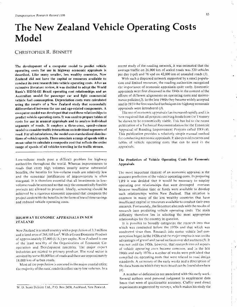
The New Zealand Vehicle Operating CostsModelCHnrsropnrn R. BrNNerr

The development of a computer rnodel to predict vehicle

operating costs for use in highway econornic appraisals is

described. Like many srnaller, less wealthy countries, New

Zealand did not have the capital or resources available toconduct its own research into vehicle operating costs. After an

extensive literature review, it was decided to adopt the WorldBank's HDM-III Brazil operating cost relationships and an

Australian model for passenger car and light cornmercialvehicle fuel consurnption. Depreciation costs were calculated

using the results of a New Zealand study that successfully

differentiated between the use and age-related cornponents. Acornputer rnodel was developed that used these relationships topredict vehicle operating costs. It was used to prepare tables ofcosts for use in rnanual appraisals and to analyze individualsegrnents of roads. It ernploys a three-zone, speed-volurne

rnodel to consider traffic inter¡ctions on individual segrnents ofroad. For all calculations, the rnodel uses standardized distribu-tions of vehicle speeds. These associate a range of speeds with a

rnean value to calculate a cornposite cost that reflects the entirerange of speeds of all vehicles traveling in the traffic stream,

Low-volume roads pose a difficult problem for highwayauthorities throughout the world. Whereas improvements toroads that carry high volumes usually accrue substantialbenefits, the benefits for low-volume roads are relatively lowand the economic justification of improvements is oftenmarginal. It is therefore essential that all investments in low-volume roads be screened so that only the economically feasibleprojects are allowed to proceed. Ideally, screening should be

achieved by a rigorous economic appraisal that compares theproject costs with the benefits in the form oftravel time savings

and reduced vehicle operating costs.

HIGHWAY ECONOMIC APPRAISALS IN NEWZEALAND

New Zealand is a small country with a population of 3.3 millionand a land area of 268, 105 km2. With a Gross Domestic Productof approximately $7,000 (U.S.) per capita, New Zealand is one

of the least wealthy of the Organization of Economic Co-operation and Development countries. The major exportindustries are related to primary produce. The rural sector is

serviced by some 80,000 km ofroads and there are approximatelyI 8,000 km of urban roads.

M ost of the population is centered in the maj or coastal cities;

the majority ofthe rural roads therefore carry low volumes. ln a

Transporlation Research Record I 106 83

recent study of the roading network, it was estimated that the

average traffic on 26,000 km of sealed roads was 320 vehiclesper day (vpd) and 76 vpd on 42,000 km of unsealed roads (1).

With such a dispersed network supported by a small popula-tion and limited resources, the roading authorities recognized

the importance of economic appraisals quite early. Economicappraisals were first discussed in the 1940s in the context of the

effects of different alignments on operating costs and mainte-

nance policies (2). I n the late I 9ó0s they became widely accepted

and in 197 I the first standard techniques for highway economic

appraisals were introduced (3).

The use of economic appraisals has increased rapidly and it is

now required that all projects receiving funds from the Treasury

be shown to be economically viable. This has led to the recent

publication of a Technical Recommendation for the EconomicAppraisal of Roading Improvement Projects called TR9 (4).

This publication provides a relatively simple manual methodfor conducting economic appraisals. lt also provides curves and

tables of vehicle operating costs that can be used in theappraisals.

The Prediction of Vehicle Operating Costs for Econornic

,4.ppraisals

The most important element of an economic appraisal is the

accurate prediction ofthe vehicle operating costs. ln preparing

TR9 it was decided that it would be necessary to employ

operating cost relationships that were developed overseas

because insufficient time or funds were available to develop

such relationships within New Zealand. This situation is

common in many of the less wealthy countries that have

insufficient capital or resources available to conduct their own

research. Fortunately, the literature abounds with the results ofresearch into predicting vehicle operating costs. The maindifficulty therefore lies in selecting the most appropriaterelationships for the country in question.

It is possible to broadly categorize the research into thatwhich was conducted before the 1970s and that which was

conducted since then. Research into motor vehicle fuel con-

sumption began in the 1920s and the major emphasis was on the

advantages of gravel and paved surfaces over d irt surfaces (5). I twas not until the 1950s, however, that research into all aspects

of vehicle operating costs became common, and in the late

1960s and early 1970s a number of works were published thatcompiled the operating costs that were related to road design

standards. A summary of the early works and a description ofthe data bases on which they were based can be found elsewhere

(6).

A number of deficiencies are associated with this early work.Several authors used personal judgment to supplement data

bases that were of questionable accuracy. Claffey used directexperiments augmented by surveys, which makes his study theW. D. Scott Deloitte Ltd., P.O. Box 2459, Auckland, New Zealand.

84

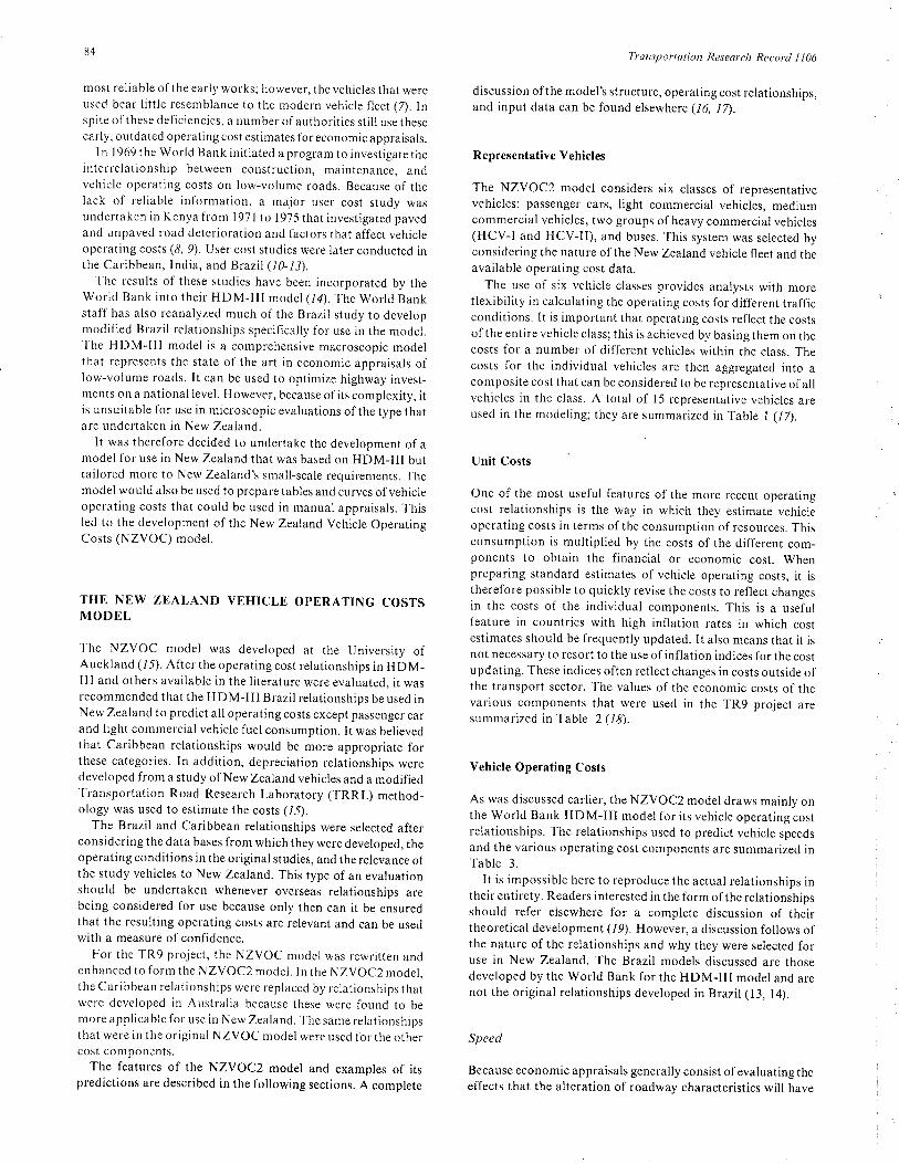
most reliable of the early works; however, the vehicles that wereused bear little resemblance to the modern vehicle fleet (Z). Inspite ofthese deficiencies, a number ofauthorities still use theseearly, outdated operating cost estimates for economic appraisals.

I n I 969 the World Bank initiated a program to investigate theinterrelationship between construction, maintenance, andvehicle operating costs on low-volume roads. Because of thelack of reliable information, a major user cost study wasundertaken in Kenya from I 97 I to I 975 that investigated pavedand unpaved road deterioration and factors that affect vehicleoperating costs (8, 9). User cost studies were later conducted inthe Caribbean, India, and Brazil (10-/,3).

The results of these studies have been incorporated by theWorld Bank into their HDM-lll model (14). The World Bankstaff has also reanalyzed much of the Brazil study to developmodified Brazil relationships specifically for use in the model.The HDM-lII model is a comprehensive macroscopic modelthat represents the state of the art in economic appraisals oflow-volume roads. It can be used to optimize highway invest-ments on a national level. However, because of its complexity, itis unsuitable for use in microscopic evaluations of the type thatare undertaken in New Zealand.

It was therefore decided to undertake the development ofamodel for use in New Zealand that was based on HDM-III buttailored more to New Zealand's small-scale requirements. Themodel would also be used to prepare tables and curves ofvehicleoperating costs that could be used in manual appraisals. Thisled to the development of the New Zealand Vehicle OperatingCosts (NZVOC) model.

THE NEW ZEALAND VEHICLE OPBRATING COSTSMODBL

The NZVOC model was developed at the University ofAuckland (15). After the operating cost relationships in HDM-III and others available in the literature were evaluated, it wasrecommended that the HDM-IIt Brazil relationships be used inNew Zealand to predict all operating costs except passenger carand light commercial vehicle fuel consumption. It was believedthat Caribbean relationships would be more appropriate forthese categories. In addition, depreciation relationships weredeveloped from a study of New Zealand vehicles and a modifiedTransportation Road Research Laboratory (TRRL) method-ology was used to estimate the costs (15).

The Brazil and Caribbean relationships were selected afterconsidering the data bases from which they were developed, theoperating conditions in the original studies, and the relevance ofthe study vehicles to New Zealand. This type ofan evaluationshould be undertaken whenever overseas relationships arebeing considered for use because only then can it be ensuredthat the resulting operating costs are relevant and can be usedwith a measure of confidence.

For the TR9 project, the NZVOC model was rewritten andenhanced to form the NZVOC2 model. ln the NZVOC2 model,the Caribbean relationships were replaced by relationships thatwere developed in Australia because these were found to bemore applicable for use in New Zealand. The same relationshipsthat were in the original NZVOC model were used for the othercost components.

The features of the NZVOC2 model and examples of itspredictions are described in the following sections. A complete

Tt'ansportation Research Record I t06

discussion ofthe model's structure, operating cost relationships,and input data can be found elsewhere (16, In.

Representative Yehicles

The NZVOC2 model considers six classes of representativevehicles: passenger cars, light commercial vehicles, mediumcommercial vehicles, two groups of heavy commercial vehicles(HCV-I and HCV-II), and buses. This system was selected byconsidering the nature of the New Zealand vehicle fleet and theavailable operating cost data.

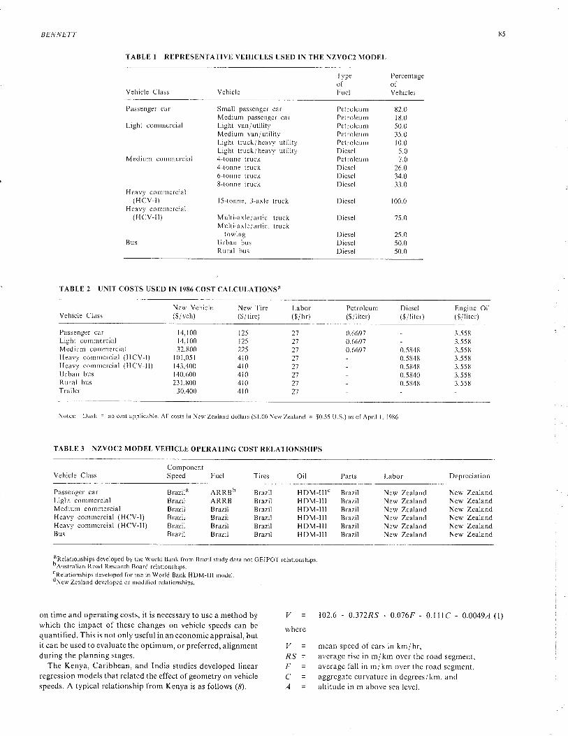
The use of six vehicle classes provides analysts with moreflexibility in calculating the operating costs for different trafficconditions. It is important that operating costs reflect the costsofthe entire vehicle class; this is achieved by basing them on thecosts for a number of different vehicles within the class. Thecosts for the individual vehicles are then aggregated into acomposite cost that can be considered to be representative ofallvehicles in the class. A total of l5 representative vehicles areused in the modeling; they are summarized in Table I (12).

Unit Costs

One of the most useful features of the more recent operatingcost relationships is the way in which they estimate vehicleoperating costs in terms of the consumption of resources. Thisconsumption is multiplied by the costs of the different com-ponents to obtain the financial or economic cost. Whenpreparing standard estimates of vehicle operating costs, it istherefore possible to quickly revise the costs to reflect changesin the costs of the individual components. This is a usefulfeature in countries with high inflation rates in which costestimates should be frequently updated. It also means that it isnot necessary to resort to the use ofinflation indices for the costupdating. These indices often reflect changes in costs outside ofthe transport sector. The values of the economic costs of thevarious components that were used in the TR9 project aresummarized in Table 2 (18).

Vehicle Operating Costs

As was discussed earlier, the NZVOC2 model draws mainly onthe World Bank HDM-III model for its vehicle operating costrelationships. The relationships used to predict vehicle speedsand the various operating cost components are summarized inTable 3.

It is impossible here to reproduce the actual relationships intheir entirety. Readers interested in the form ofthe relationshipsshould refer elsewhere for a complete discussion of theirtheoretical development (/9). However, a discussion follows ofthe nature of the relationships and why they were selected foruse in New Zealand. The Brazil models discussed are thosedeveloped by the World Bank for the HDM-III model and arenot the original relationships developed in Brazil (13, l4).

Speed

Because economic appraisals generally consist of evaluating theeffects that the alteration of roadway characteristics will have

BEN NETT 85

TABLE I REPRESENTATIVE VEHICLES USED IN THE NZVOC2 MODEL

Type Percentageof ofFuel VehiclesVehicle Class Vehicle

Passenger car Small passenger car Petroleum 82.0Medium passenger car Petroleum 18.0

Light commercial Light van/utility Petroleum 50.0Medium van/utility Petroleum 35-0Light truck/heavy utility Petroleum 10.0Light truck/heavy utility Diesel 5.0

Medium commercial 4-tonne truck Petroleum 7.04-tonne truck Diesel 26.06-tonne truck Diesel 34.08-tonne truck DieseÌ 33.0

Heavy commercial(HCV-I) I5-tonne,3-axle truck Diesel 100.0

Heavy commercial(HCV-ll) Multi-axle/artic. truck DieseÌ 75.0

Multi-axle/ artic. trucktowing Diesel 25.0

Bus Urban bus Diesel 50.0Rural bus Diesel 50.0

TABLE 2 UNIT COSTS USED IN I986 COST CALCULATIONSå

Vehicle ClassNew Vehicle New Tire Labor Petroleum Diesel Engine Oil($/veh) ($/tire) ($/hr) (g/liter) (g/liter) (g/liter)

Passenger carLight commercialMedium commercialHeavy commercial (HCV-I) l0l,05l 4t0Heavy commercial (HCV-ll) 143,400 410

14,100 12514,100 t2532.800 225

0.66970.6697

272727

2727272727

3.5583.558

Urban busRural busTrailer

140,600 41023 t,800 41030,400 410

0.6697 0.5848 3.558- 0.5848 3.558- 0.5848 3.558- 0.5840 3.558- 0.5848 3.558

Notes: Dash : no cost applicable. All costs in New Zealand dollars (91.00 New Zealand = $0.55 U.S.) as ofApril l, 1986

TABLE 3 NZVOC2 MODEL VEHICLE OPERATING COST RELATIONSHIPS

Vehicle ClassComponentSpeed Fuel Tires Oil Parts Labor Depreciation

Passenger carLight commercialMedium commercial

Brazila ARRBb Brazil HDM-Illc Brazil New Zealand New ZealandBrazl ARRB Brazil HDM-lll Brazil New Zealand New ZealandBrazil Brazil Brazil HDM-lll Brazil New Zealand New Zealand

Heavy commercial (HCV-I) Brazil Brazil Brazil HDM-lll Brazil New Zealand New ZealandHeavy commercial (HCV-I|) Brazil Brazil Brazil HDM-III Brazil New Zealand New ZealandBus Brazil Brazil Brazil HDM-lll Brazil New Zealand New Zealand

fRelationships developed by the World Bank from Brazil study data not GEIPOT relationships.uAustralian Road Research Board relationships.

lRelationships developed for use in World Bank HDM-lll model.oNew Zealand developed or modified relationships.

ontimeandoperatingcosts,itisnecessarytouseamethodby V -- 102.6 - 0.372-RS - 0.076F - 0. lllC - 0.00491 (l)which the impact of these changes on vehicle speeds can be wherequantified. This is not only useful in an economic appraisal, butit can be used to evaluate the optimum, or preferred, alignment I't = mean speed of cars in kmi hr,during the planning stages, ¡RS = average rise in m/km over the road segment,

The Kenya, Caribbean, and India studies developed linear F = average fall in m/km over the road segment,regression models that related the effect ofgeometry on vehicle C = aggregate curvature in degrees/km, andspeeds. A typical relationship from Kenya is as follows (8). A = altitude in m above sea level.

86

A complete set of equations is given in a study by Bennett inwhich their predictions are discussed and compared (/5).

Regression equations of this nature have two major short-comings (20). An inconsistency exists in the coefficients between

the equations from the various studies, which is partly a resultof the high degree of correlation between road characteristics.Curves and grades are often found together and the regressionprocedure may not correctly isolate the independent effects ofcurves and grades.

The second shortcoming is that the regression equations are

unable to handle extreme conditions. It is possible to obtainnegative values of speed for reasonable combinations of roadcharacteristics. Furthermore, the geometric effects have a

constant effect regardless of the values of other geometricfeatures. This means, ior example, that speeds on a steep

upgrade could be increased by making the surface smoothereven though the gradient is the speed-limiting factor and not thesurface condition (20).

The World Bank developed an alternative method of modelingspeed-geometry effects for the H DM-l II model using data fromthe Brazil study (/9). The method assumes that each vehicle has

a set of limiting maximum speeds for open roads, upgrades,downgrades, curves, and rough surfaces. At any given point, the

speed will be the minimum of these five values.

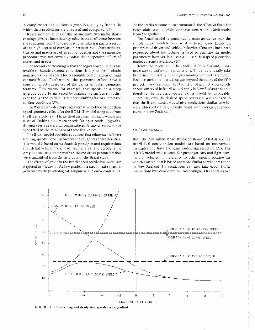
The Brazil model provides equations that relate each oftheselimiting speeds to road geometry and roughness characteristics.The model is based on mechanistic principles and requires datathat detail vehicle mass, load, frontal area, and aerodynamicdrag. It also uses a number ofvehicle and driver parameters thatwere quantified from the field data of the Brazil study.

The effects of grade in the Brazil speed prediction model are

depicted in Figure l. At low grades, the steady state speed is

governed by the psychological, roughness, and curve constraints.

Transportation Research Record I 106

As the grades become more pronounced, the effects ofthe otherconstraints lessen until the only constraint is that which results

from the gradient.

The Brazil model is conceptually more attractive than the

simple linear models because it is based more firmly onprinciples of driver and vehicle behavior. Concerns have been

expressed about the techniques used to quantify the modelparameters; however, it still constitutes the best speed predictionmodel currently availabte (20).

Before the model could be applied in New Zealand, it was

necessary to calibrate its predictions. This should ideally takethe form of requantifying all regression-based model parameters.

Because such an undertaking was beyond the scope ofthe TR9project, it was assumed that the effect of geometry on vehiclespeeds observed in Brazil would apply in New Zealand and thattherefore the regression-based values would be applicable.Therefore, only the desired speed constraint was changed so

that the Brazil model would give predictions similar to whatwere observed on flat, straight roads with average roughness

levels in New Zealand.

Fuel Consumption

Both the Australian Road Research Board (ARRB) and the

Brazil fuel consumption models are based on mechanisticprinciples and have the same underlying structure (21). TheARRB model was selected for passenger cars and light com-mercial vehicles in preference to other models because thevehicles on which it is based are more similar to what are foundin New Zealand. Its predictions can also take urban trafficinteractions into consideration. Accordingly, TR9 contains two

,CONSTRAINING ROUGHNISS SPEED

- - _J1- -----h_----\CONSTRAINING CURVE SPEED

CONSTR,A IN ING DES IRED SPEED

/DO\{NH I LL SPEED+//

,,

_/=.E

¿)uôUgc- ¿n

CONSTRqINING

60

70 CCìISTRAINING UPHI LL SPEED

,/\

GRADIENT IN PERCENT

FIGURE I Constraining rnd steady-strte speeds versus gradient.

/

tl-4-6-õl0

PREDICTED STEADY STATE SPEED

BENNETT

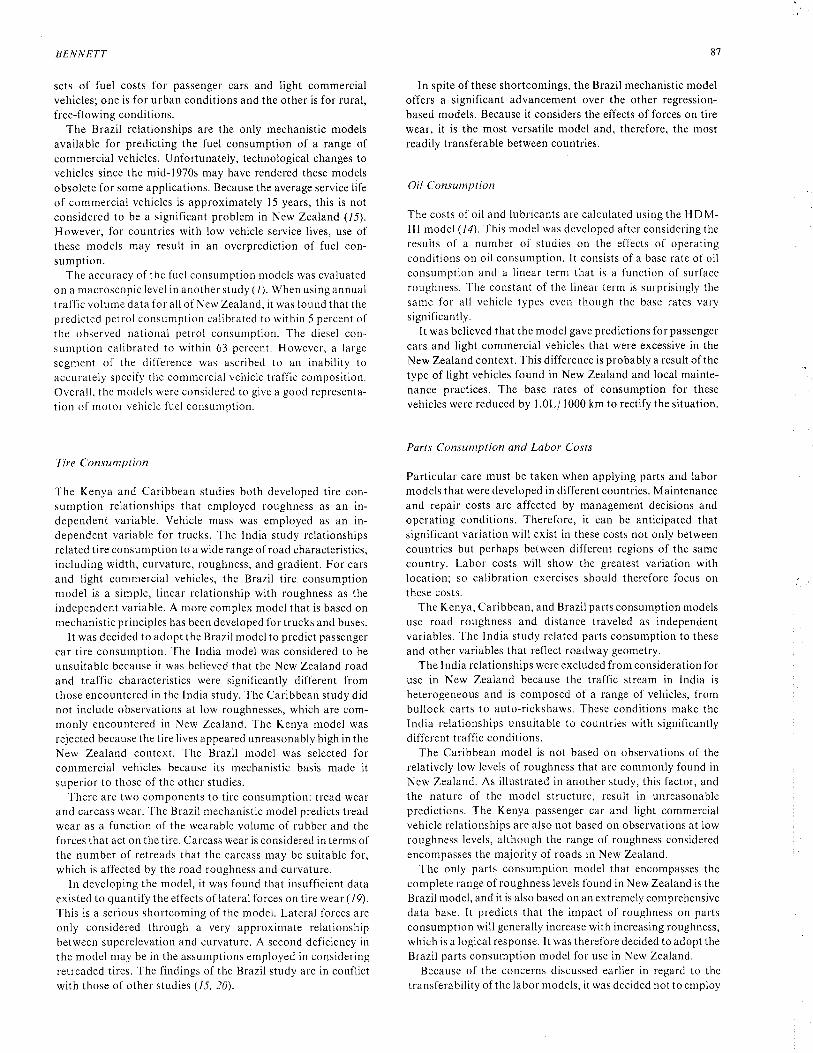
sets of fuel costs for passenger cars and light commercialvehicles; one is for urban conditions and the other is for rural,free-fl owing conditions.

The Brazil relationships are the only mechanistic modelsavailable for predicting the fuel consumption of a range ofcommercial vehicles. Unfortunately, technological changes tovehicles since the mid-1970s may have rendered these modelsobsolete for some applications. Because the average service lifeof commercial vehicles is approximately l5 years, this is notconsidered to be a significant problem in New Zealand (15).

However, for countries with low vehicle service lives, use ofthese models may result in an overprediction of fuel con-sumption.

The accuracy of the fuel consumption models was evaluatedon a macroscopic level in another study (/). When using annualtraffic volume data for all of New Zealand, it was found that thepredicted petrol consumption calibrated to within 5 percent ofthe observed national petrol consumption. The diesel con-sumption calibrated to within 63 percent. However, a large

segment of the difference was ascribed to an inability toaccurately specify the commercial vehicle traffic composition.Overall, the models were considered to give a good representa-tion of motor vehicle fuel consumption.

Tire Consumption

The Kenya and Caribbean studies both developed tire con-sumption relationships that employed roughness as an in-dependent variable. Vehicle mass was employed as an in-dependent variable for trucks. The India study relationshipsrelated tire consumption to a wide range of road characteristics,including width, curvature, roughness, and gradient. For cars

and light commercial vehicles, the Brazil tire. consumptionmodel is a simple, linear relationship with roughness as theindependent variable. A more complex model that is based onmechanistic principles has been developed for trucks and buses.

It was decided to adopt the Brazil model to predict passenger

car tire consumption. The India model was considered to be

unsuitable because it was believed that the New Zealand roadand traffic characteristics were significantly different fromthose encountered in the India study. The Caribbean study didnot include observations at low roughnesses, which are com-monly encountered in New Zealand. The Kenya model was

rejected because the tire lives appeared unreasonably high in theNew Zealand context. The Brazil model was selected forcommercial vehicles because its mechanistic basis made itsuperior to those of the other studies.

There are two components to tire consumption: tread wearand carcass wear. The Brazil mechanistic model predicts treadwear as a function of the wearable volume of rubber and theforces that act on the tire. Carcass wear is considered in terms ofthe number of retreads that the carcass may be suitable for,which is affected by the road roughness and curvature.

In developing the model, it was found that insufficient dataexisted to quantify the effects oflateral forces on tire wear (19).

This is a serious shortcoming of the model. Lateral forces are

only considered through a very approximate relationshipbetween superelevation and curvature. A second deficiency inthe model may be in the assumptions employed in consideringretreaded tires. The findings of the Brazil study are in conflictwith those of other studies (15, 20).

87

In spite of these shortcomings, the Brazil mechanistic modeloffers a significant advancement over the other regression-based models. Because it considers the effects of forces on tirewear, it is the most versatile model and, therefore, the mostreadily transferable between countries.

Oil Consumption

The costs of oil and lubricants are calculated using the H D M-III model (14). This model was developed after considering theresults of a number of studies on the effects of operatingconditions on oil consumption. It consists of a base rate of oilconsumption and a linear term that is a function of surfaceroughness. The constant of the linear term is surprisingly the

same for all vehicle types even though the base rates varysignificantly.

It was believed that the model gave predictions for passenger

cars and light commercial vehicles that were excessive in theNew Zealand context. This difference is probably a result ofthetype of light vehicles found in New Zealand and local mainte-nance practices. The base rates of consumption for these

vehicles were reduced by I .0L/ 1000 km to rectify the situation.

Parts Consumption and Labor Costs

Particular care must be taken when applying parts and labormodels that were developed in different countries. Maintenanceand repair costs are affected by management decisions andoperating conditions. Therefore, it can be anticipated thatsignificant variation will exist in these costs not only between

countries but perhaps between different regions of the same

country. Labor costs will show the greatest variation withlocation; so calibration exercises should therefore focus onthese costs.

The Kenya, Caribbean, and Brazil parts consumption modelsuse road roughness and distance traveled as independentvariables. The India study related parts consumption to these

and other variables that reflect roadway geometry.

The India relationships were excluded from consideration foruse in New Zealand because the traffic stream in lndia is

heterogeneous and is composed of a range of vehicles, frombullock carts to auto-rickshaws. These conditions make theIndia relationships unsuitable to countries with significantlydifferent traffic conditions.

The Caribbean model is not based on observations of the

relatively low levels of roughness that are commonly found inNew Zealand. As illustrated in another study, this factor, andthe nature of the model structure, result in unreasonablepredictions. The Kenya passenger car and light commercialvehicle relationships are also not based on observations at lowroughness levels, although the range of roughness consideredencompasses the majority of roads in New Zealand.

The only parts consumption model that encompasses thecomplete range of roughness levels found in New Zealand is theBrazil model, and it is also based on an extremely comprehensivedata base. It predicts that the impact of roughness on partsconsumption will generally increase with increasing roughness,

which is a logical response. lt was therefore decided to adopt theBrazil parts consumption model for use in New Zealand.

Because of the concerns discussed earlier in regard to thetransferability of the labor models, it was decided not to employ

88

a labor model that was developed in one ofthe user cost studies.It has been suggested that the ratio of parts to labor costs lies inthe range of 50:50 to 60:40 (22).The approach adopted was tohave a constant cost based on a 55:45 split between parts andlabor costs. This value was selected because parts in NewZealand comprise a slightly larger portion of the total mainte-nance and repair costs than labor.

Unlike the other component costs, estimates of maintenanceand repair costs based on New Zealand surveys were available.It was clearly desirable to calibrate the Brazil parts consumptionmodel so that its predictions were the same as these knownvalues at average roughness values. Two methods were availablefor .calibrating the model; the model parameters could bemodified or a constant term, which may be negative, could beadded to the predictions. As was illustrated in another study,the latter is the only appropriate method, because it does notaffect the impact of the independent variables on the modelpredictions (/5).

The parts model was therefore calibrated by first determiningthe parts component of the New Zealand costs based on the55:45 split between parts and labor costs. A constant term was

then added to the Brazil model predictions so that they gave thesame values at an average roughness level.

Depreciatíon

The depreciation expense ofa motor vehicle arises as a result ofusage, age, and technological obsolescence. The use-relateddepreciation should be treated as a running cost. The age andtechnological obsolescence costs are overhead costs becausethey occur independently ofvehicle use. ForTR9, the deprecia-tion costs are calculated using the relationships and methodologyestablished in another study (1J). It was found that passenger

car and commercial vehicle depreciation could be predictedusing relationships of the following form:

Passenger cars: DEP = C (AGÐ^ (KILOIuDB Q)Commercial vehicles: DEP = C - D (AGÐ^ 6ILO^48 (3)

where

DEP

AGEKILOMAtoD

= depreciation of a vehicle as a percentage ofthe vehicle replacement price,

= age of vehicle in years,

= cumulative kilometrage of vehicles, and

= constants.

These depreciation relationships were established using thefollowing methodology:

. Data on recent resale values of motor vehicles, and theirage and distance traveled, were collected from newspapers anddealers'guides.

r The original retail value of vehicles was determined andinflated into current dollars.

¡ The depreciation (as a percentage) is the differencebetween the inflated original value and the recent resale value.

¡ An SAS nonlinear regression package was used to relatethe vehicle depreciation to its age and distance traveled(constants A to D in Equations 2 and 3) (23).

Transportation Research Record I 106

The use ofthese relationships in conjunction with the age andcumulative kilometrage data enable the value of a vehicle at anystage of its life to be calculated. These data can then be

aggregated to provide a single value to express depreciationcosts for the fleet. This process can be mathematically expressed

as follows (/7):

n

DEPCOF= f FREQ.CDEP.i=l

(4)

The variable CDEPiis defined as follows:

CDEPi = DEP¡- DEP.- |

The annual depreciation costs are obtained by multiplyingthe depreciation coefficient by the replacement price of a

vehicle.The weighting of the exponents in the depreciation relation-

ships gives the relative percentages ofthe total depreciation thatresult from use and age. The following are percentages of thetotal depreciation that results from vehicle use: passenger

cars-40 percent, light commercial vehicles 30 percent, othercommercial vehicles 20 percent, and buses-20 percent.

Vehicle Speeds

Economic appraisal techniques generally have not adequatelyconsidered the sensitivity ofvehicle operating costs, particularlyfuel costs, to operating speeds. The standard practice is toestimate the mean speed of the traffic stream using models suchas those discussed earlier and then calculate the vehicleoperating costs that correspond to this speed.

This practice ignores the fact that the average speed ol'vehicles on a road is composed of a distribution of speeds. Thecosts that correspond to each speed in the distribution should be

calculated and then combined to form a composite speed costfor a stream of vehicles with a given mean speed. This compositecost can be calculated using the following relationship (12):

n

> cosTi SPFR,i=l

where

DEPCOFFREQiCDEPi

COMCOST =

where

COMCOST

cosrisPFÀ,

n

= depreciationcoefficient,

= percentage of vehicle of age i in the fleet, and

= change in depreciation over year i.

the composite speed costs for a stream oftraffic with a mean speed of Z,

the cost of a vehicle traveling at speed l,the number ofvehicles in the stream travelingat speed i, andthe number of different speeds in thedistribution.

(5)

(6)

As was discussed in another study, when individual spotspeed observations in a sample are divided by the sample mean

89BENNETT

r00

90

80

u70Ots=360ÍUÈu50;Íqa-ã-tfo

70

lo

o. ¿ 0.6 0.6 1.0

R,ATIO OF OBSERVED SPIED

FIGURE 2 Standardized passenger car speed distribution.

1.2

TO MEAN SPEED

1.6

SQ¡ = S¡ 8H R<QO (7)

SQ¡ = S¡- (SC,4 P)(QHR-QO)I@CAP-QO)Q}<QH R'<QCA P (8)

SQ¡ = SCAP - (SCAP'SJA tví)(QH R-QCAP)l(QJAM-QCA P) SCAP<QHR<QJAM (e)

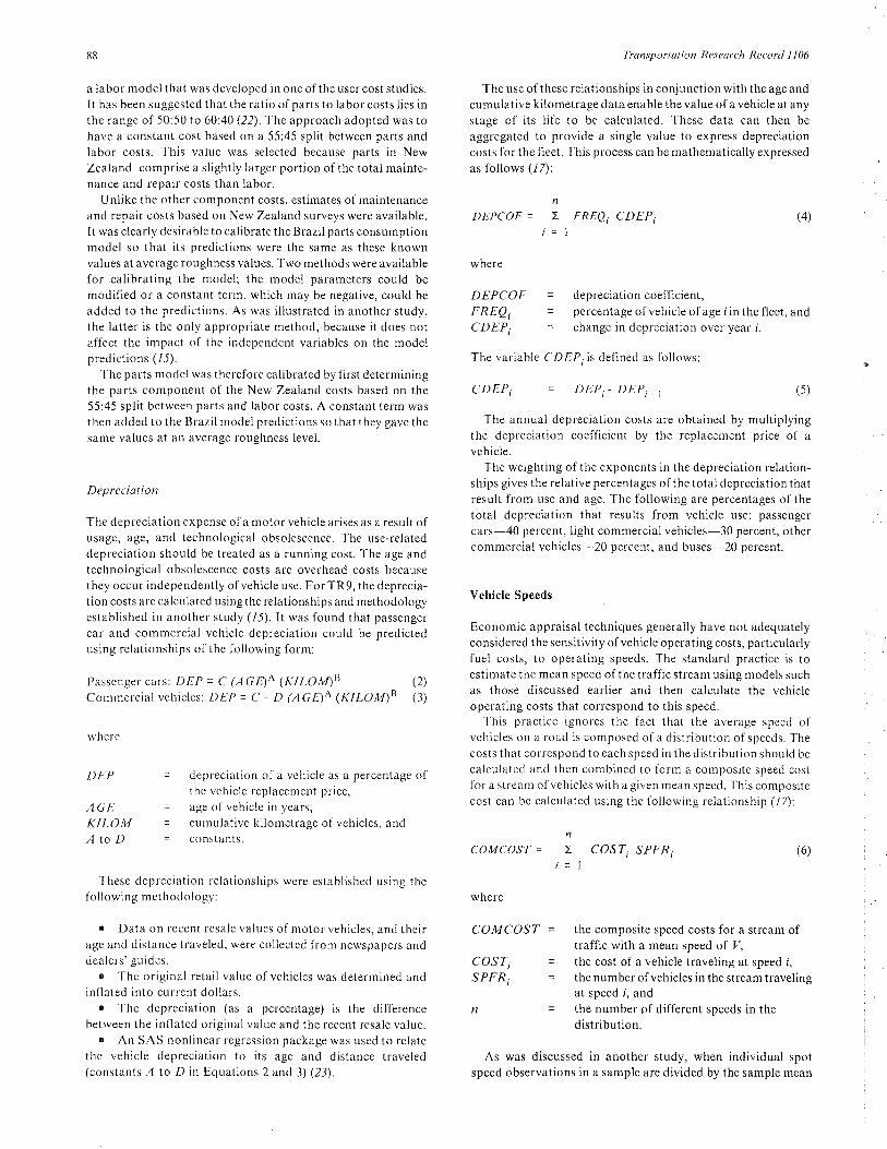
speed, the resulting standardized distribution is identical tostandardized distributions from other sites (24). Data from six

spot speed studies that were conducted throughout New

Zealand were used to establish standardized distributions fornine different vehicle classes. Figure 2 is an example of the

standardized passenger car distribution (24).

Standardized distributions make it possible to fully describe

the speed distribution solely from the mean speed. They provide

details of the the range of speeds associated with the mean value

and also of the number of vehicles that can be found over the

range. Given a mean speed, which can either be predicted using

the Brazil speed prediction model or estimated by the user, the

NZVOC2 model uses the appropriate standardized speed

distribution for the vehicle class to calculate the composite

speed costs. This results in differences in fuel costs of up to l0percent over those associated with the mean speed.

Speed-Volurne Effects

Speed-volume effects are an important consideration in eco-

nomic appraisals. Traffic delays on rural roads are usually

associated with the supply and demand of overtaking op-

portunities. The demand often cannot be met and vehicles are

forced to travel at the speed ofthe slowest vehicle until a passing

opportunity presents itself.The literature is summarized in another study that suggests

that speed-volume effects for one vehicle type depend on the

free speeds of other vehicle types (20). It goes on to suggest the

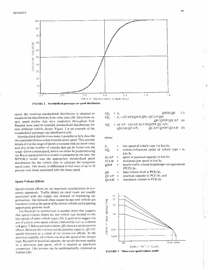
use of a three-zone speed-volume relationship such as is shown

in Figure 3. Below a certain volume, Q0,thete areno interaction

effects. Between this volume and the practical capacity, 8CA P'

speeds decrease as a result of the interaction effects. At the

practical capacity, all vehicles travel at the speed of the slowest

type. Beyond the practical capacity, the speeds decrease rapidly

to a minimum .iam speed, which is reached at maximum

congestion. This process can be mathematically expressed as

follows (20):

= free speed of vehicle type i in km/hr,= volume-influenced speed of vehicle type i in

km/ hr,speed at practical capacity in km/hr,minimum jam speed in km/hr,hourly trafficvolume in passenger car equivalents(PCE)/hr,base volume level in PCE/hr,practical capacity in PCE/hr, and

maximum volume in PCE/hr.

where

s,SQi

SCAP =

SJAM =

QHR =

Qo=QCAP =

QJAM

SI

u52L

F ..)C)

-U=s4IOU

o

3 scAPUL

SJ Al"l

Q0

I.IOLJRLY -IRAII' IC VOLU¡48

FIGURE 3 Three'zone speed-volume model.

QCAP QJI\NI

SCAP =

where

covi

90

It is recommended that SCAP be quantified as the l5thpercentile speed of the slowest vehicle (20). Because speedsgenerally are normally distributed, this value can be approx-imated by the mean-minus-one standard deviation. Values forthe coefficient of variation of vehicle speeds (defined as themean divided by the standard deviation) that are based on NewZealand studies are given in another sfidy (24). The speed atcapacity is therefore calculated as follows:

Transportation Reseorch Record I 106

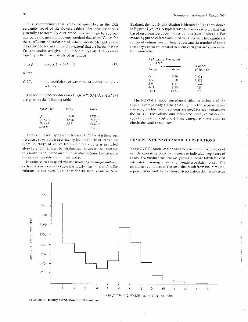
Zealand, the hourly distribution is bimodal of the form shownin Figure 4 (25, 26).A typical distributionwas selected that wasbased on a consideration ofdistributions from I I sites (1). Formodeling purposes it was assumed that there were five signifìcantranges of volume levels. These ranges and the number of hoursthat they can be anticipated to occur each year are given in thefollowing table.

Volumes as Petrcntageof AADT

Nuntberof Hrsl Yr

2,294t {'tt3,524

3555t

The NZVOC2 model therefore divides an estimate of theannual average daily traffic (AADT) into five represenrarivevolumes, establishes the appropriate speed for each volume onthe basis of the volume and mean free speed, calculates thevehicle operating costs, and then aggregates these costs toobtain the total annual cost.

EXAMPLES OF NZVOC2 MODEL PREDICTIONS

The NZVOC2 model can be used to provide standard tables ofvehicle operating costs or to analyze individual segments ofroads. The model provides two types ofstandard tabulated costestimates: running costs and roughness-related costs. Theformer are composed of the costs that result from fuel, tires, oil,repairs, labor, and that portion ofdepreciation that results from

min[S¡ (l - COVí)) ( l0)

= the coefficient of variation of speeds for type I

vehicles-

Range

0-lt-55-99-l I

>lt

Mean

0.502.586.879.80I L66

The recommended values for Q0,8CA P, QJA M, and SJA Mare given in the following table.

Paranteter Value Unit.t

PCE hrPCE¡ hrPCE ¡ hrkm¡ hr

These values are ex p lessed i n terms of PC E / hr; it is thereforenecessary to establish equivalency factors for the other vehicletypes. A range of values from different studies is providedelsewhere (20). lf must be emphasized, however, that becausethis model is not based on empirical observations, the values inthe preceding table are only estimates.

I n order to use the speed-volume modeling technique outlinedearlier, it is necessary to know the hourly distribution of trafficvolume. lt has been found that for all rural roads in New

2250

2000

r 750

r 500

1250

I 000

150

500

250

) 6 7 I 9 ì0 I

HOURLY TRAFFIC VOLUI,4E AS PERCENT OF AADT

Q0QMAXQJA MSJA M

I002.5003.125

IJ

g:

U

Éuro-

Ø(tlaIÕúufn=lz

FIGURE 4 Hourly distribution of traffic volurne,

BEN N ETT

vehicle use. The latter constitute the additional costs that resultfrom changing roughness levels. Each of these costs is discussedindividually.

Five significant independent variables were used in thecalculation of the running costs. In increasing order of im-portance they are altitude, curvature, roughness, gradient,_andspeed.

The altitude affects the operating costs through its effects onthe mass density of air. lt has a very minor impact that amountsto less than I percent over the entire range of altitudes in NewZealand. Because of this insensitivity, all costs were calculatedusing a value of l0 m above sea level for the altitude.

The main impact of curvature on operating costs is throughits effect on vehicle speeds. In terms of a direct effect onoperating costs, only commercial vehicle tire consumption is

affected by curvature. The running costs were calculated using a

constant value of l0 degrees/km for curvature.Roughness is an important variable, as evidenced by its

inclusion in each of the HDM-llI model relationships. Un-fortunately, the Australian Road Research Board (ARRB) wasconcentrating on urban traffic management; therefore, surfaceroughness is not incorporated in the ARRB fuel consumptionmodel. In calculating the running costs, it was decided toeliminate the roughness effects by having all costs calculated ata roughness of zero National Association of Australian StateRoad Autho¡ities (NAASRA) counts/km. Separate roughnesscosts could then be added to these base costs to establish thetotal vehicle operating costs. Because the HDM-lll model uses

the QI roughness measure, whereas in New Zealand roughness

lE0

r53

t!¡

9l

is measured using a NAASRA Meter, it was necessary toconvert NAASRA counts to QI counts (27). This was doneusing the following approximate relationship (12).

8r = (46.7 + NAASRA)12.761

where

(l l)

180

l?0

NAASRAQr

ì MCV

SURFÂCE ROUGHNESS IN NAÁSRA COUNfSfiM

It must be stressed that this is a very approximate relationshipbased on estimates of the relationship between the NAASRAMeter and the TRRL Bump Integrator and the Bump Integratorand the QI measure. The Ministry of Works and Developmentundertook field studies to quantify a more exact relationship;however, there were errors in the data. It is hoped that theseerrors will be resolved and that a more accurate relationship willbe available in the near future.

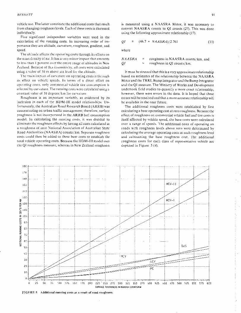
The additional roughness costs were established by firstcalculating a base operating cost at zero roughness. Because theeffect of roughness on commercial vehicle fuel and tire costs is

itself affected by vehicle speed, the base costs were calculatedover a range of speeds. The additional costs of operating onroads with roughness levels above zero were determined bycalculating the average operating costs at each roughness leveland subtracting the base roughness cost. The additionalroughness costs for each class of representative vehicle aredepicted in Figure 5 (4).

= roughness in NAASRA counts/km, and

= roughness in QI counts/km.

133

=s r?0ô

Þil0U2 tñ',

F

osco2".="-lcr-¿''zÊe.oêosi

ti -i

qs0175ls0125r0050?5 200 2?5' 250 2i5 300 325 350 375

FIGURE 5 Additional running costs as a result ofroad roughness.

q75 :,25 550 575 500

92

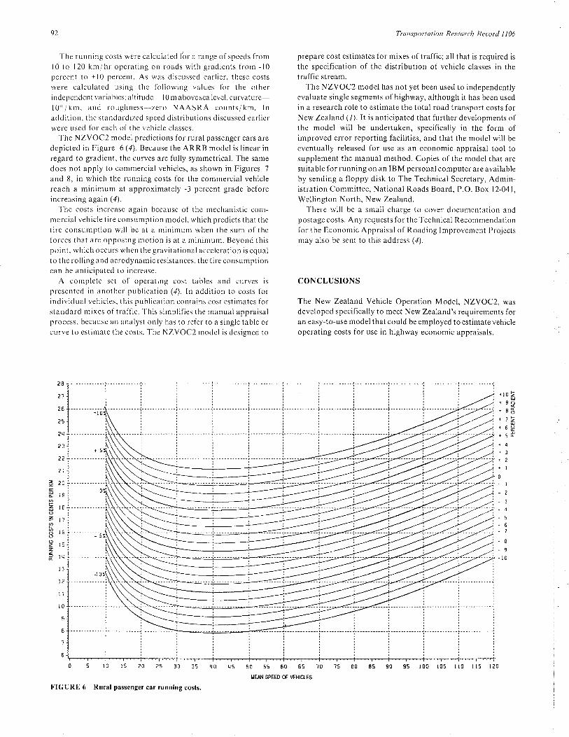
The running costs were calculated fòr a range of speeds froml0 to 120 km/hr operating on roads with gradients from -10percent to +10 percent. As was discussed earlier, these costs

were calculated using the following values for the otherindependent variables: altitude l0 m above sea level, curvaturel0o/km, and roughness zero NAASRA counts/km. Inaddition. the standardized speed distributions discussed earlierwere used for each of the vehicle classes.

The NZVOC2 model predictions for rural passenger cars aredepicted in Figure 6 (4). Because the ARRB model is linear inregard to gradient, the curves are fully symmetrical. The same

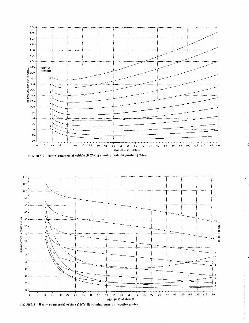
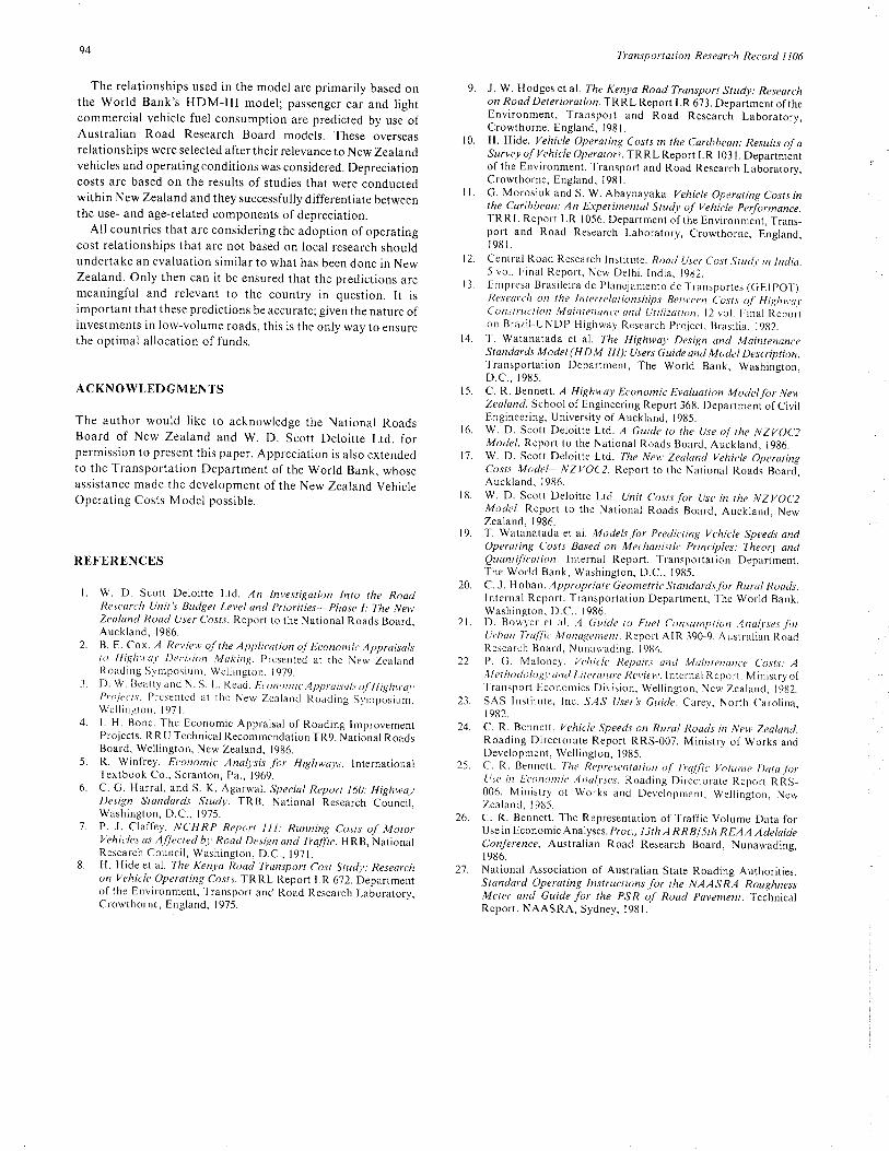
does not apply to commercial vehicles, as shown in Figures 7and 8, in which the running costs for the commercial vehiclereach a minimum at approximately -3 percent grade beforeincreasing again (4).

The costs increase again because of the mechanistic com-mercial vehicle tire consumption model, which predicts that thetire consumption will be at a minimum when the sum of theforces that are opposing motion is at a minimum. Beyond thispoint. which occurs when the gravitational acceleration is equalto the rolling and aerodynamic resistances, the tire consumptioncan be anticipated to increase.

A complete set of operating cost tables and curves is

presented in another publication (4). ln addition to costs forindividual vehicles. this publication contains cost estimates forstandard mixes of traffic. This simplifies the manual appraisalprocess, because an analyst only has to refer to a single table orcurve to estimate the costs. The NZVOC2 model is designed to

+l

Transportation Researcl't Record I I 06

prepare cost estimates for mixes of traffic; all that is required is

the specification of the distribution of vehicle classes in thetraffic stream.

The NZVOC2 model has not yet been used to independentlyevaluate single segments of highway, although it has been usedin a research role to estimate the total road transport costs forNew Zealand (1). It is anticipated that further developments ofthe model will be undertaken, specifically in the form ofimproved error reporting facilities, and that the model will beeventually released for use as an economic appraisal tool tosupplement the manual method. Copies of the model that aresuitable for running on an IBM personal computer are availableby sending a floppy disk to The Technical Secretary, Admin-istration Committee, National Roads Board, P.O. Box l2-041,Wellington North, New Zealand.

There will be a small charge to cover documentation andpostage costs. Any requests for the Technical Recommendationfor the Economic Appraisal of Roading Improvement Projectsmay also be sent to this address (4).

CONCLUSIONS

The New Zealand Vehicle Operation Model, NZVOC2, wasdeveloped specifically to meet New Zealand's requirements foran easy-to-use model that could be employed to estimate vehicleoperating costs for use in highway economic appraisals.

+10

r9+8+l+6+5r4+3+2+l0

-3-4-5-6-1

-9-10

?8

¿1

?E

25

?rl

2?

?2

2i

=20É

øtsõlÊozttts

ärt9rszze ¡,;

l-:

t?

li

t0

s

I1

6

--- _ - - _ _- _ - - f _-___ _ -_. --- t - - - - ------- - -:-

| ,----+

ñ

+lc

EE¡

?ÉoFzoE

35 50 55 60 6s ?0

MEÂN SPEEO Of \iEHICT.ES

FIGURt, ó Rural passenger car running costs.

rt0 ?5 80 85 90 95

5.- 0

5?s

500

q75

r¡50

q25

q0c

37S

350

32:

3trc

215

2SC

22t

200

tl5

r50

125

t00

50

IGI

=EuèzuozÈ

82z3É

l5 20

commercial

;iII

+

;1)

,1

j

Il

I,L

0

UR

I r0

t05

100

95

90

85

ieoGÀP152o=?CF

86s9

=EolÉ!:

50

U5

t0

35

30

MEÂJ.I SPEEO OÊ VEHIC¡.ES

vehicle (HCV-II) running costs on positive grades.

-- - -- ----i---- ------j------.1=

?5 30 35 rro rl5 50 55 50 65 ?0 75 80 85 90 95 100 105 ll0 ll5 l?0

ME¡N SPEEO Of VTHICI.ES

vehicle (HCV-II) running costs on negative grades'FIGURE

94

The relationships used in the model are primarily based onthe World Bank's HDM-III model; passenger car and lightcommercial vehicle fuel consumption are predicted by use ofAustralian Road Research Board models. These overseasrelationships were selected after their relevance to New Zealandvehicles and operating conditions was considered. Depreciationcosts are based on the results of studies that were conductedwithin New Zealand and they successfully differentiate betweenthe use- and age-related components of depreciation.

All countries that are considering the adoption of operatingcost relationships that are not based on local research shouldundertake an evaluation similar to what has been done in NewZealand. Only then can it be ensured that the predictions aremeaningful and relevant to the country in question. It isimportant that these predictions be accurate; given the nature ofinvestments in low-volume roads, this is the only way to ensurethe optimal allocation of funds.

ACKNOWLEDGMENTS

The author would like to acknowledge the National RoadsBoard of New Zealand and W. D. Scott Deloitte Ltd. forpermission to present this paper. Appreciation is also extendedto the Transportation Department of the World Bank, whoseassistance made the development of the New Zealand VehicleOperating Costs Model possible.

REFERENCES

l. W. D. Scott Deloitte Ltd. An Investigation Into the RoadResearch Unir's Budget Level and Priorities phase I: The NewZealand Road User Cosls. Report to the National Roads Board.Auckland, 198ó.

2. B. E. Cox. A Review of the Application of Economic Appraísalsto Highn'a.r l)eri.sion Making. presented at the New ZealandIì.oading Symposium, Wellingron. I 979.

3. D. W. Beatty and N. S. L. Read. Ët.onontit Appraisals o/ Highn,a.rProjects. l)rcsentcd at the New Zealand Roading Symposium,Wellington, I971.

4. I. H. Bone. The Economic Appraisal of Roading ImprovementProjects. RRU Technical Recommendation TR9. National RoadsBoard, Wellington, New Zealand, 1986.

5. R. Winfrey. Economic Anal¡,sis for Híghways. InternationalTextbook Co., Scranton, Pa.,1969.

6. C. G. Harral, and S. K. Agarwal. Special Report 160: HighwayDesign Srandards Stud¡'. TRB, National Research Council,Washington, D.C., 1975.

7. P. J. Claffey. NCHRP Report lll: Running Costs of MotorVehicles as AflÞcted b.¡, Road Design and Traffic. H RB, NationalResearch Council, Washington, D.C., 1971.

8. H. Hide et al. The Ken¡'a poo¿ Transport Cost Study: Researchon Vehicle Operating Cos¡s. TRRL Report LR 672. Departmentof the Environment, Transport and Road Research Laboratory,Crowthorne, England, I975.

Transportatíon Research Record I I 06

J. W. Hodges et al. The Kenya Road Transport Study: Researchon Road DeterioraÍion.'|F.F'L Report LR ó73. Department of theEnvironment, Transport and Road Research Laboratory,Crowthorne, England, 198 l.H. Hide. Vehicle Operating Costs in the Cøribbean: Results of aSurvey of Vehicle Operators.TRRL Report LR 1031. Departmentof the Environment, Transport and Road Research Laboratory,Crowthorne. England, 1981.G. Morosiuk and S. W. Abaynayaka. Vehicle Operating Costs inthe Caribbean: An Experímental Stud¡, of Vehicte perþrmance.TRRL Report LR 1056. Department of the Environment, Trans-port and Road Research Laboratory, Crowthorne, England,1981.

Central Road Research Institute. Road Ilser Cost Stutlt in !ndia.5 vol. Final Report. New Delhi, lndia, 1982.Empresa Brasileira de Planejamento de Transportes (GElpOT).Researth otl the Interrelationships Betu'een Costs o/ Highu,a.rConstruction Maintenante and IJtilizotion. I2 vol. Final Reporton Brazil-UNDP Highway Research project, Brasilia. 19g2.T. Watanatada et al. The Highway Design and MainîenanceStandards Model(H DM-lII): IJsers Guide and Mode! Desuiption.Transportation Department, The World Bank, Washington,D.C., 1985.

C. R. Bennett. A Highwa¡,Economic Evaluatíon Modelfor NewZealand. School of Engineering Report 368. Department of CivilEngineering, University of Auckland, 1985.W. D. Scott Deloitte Ltd. A Guide to the IJse of the NZVOC2Model. Report to the National Roads Board, Auckland, I9g6.W. D. Scott Deloitte Ltd. The New Zealancl Vehit.le OperatingCosts Model-NZVOC2. Report to the National Roads Board,Auckland,1986.W. D. Scott Deloitte Lrd. Unit Costs for use in the NZVOC2Model. Report to the National Roads Board, Auckland, NewZealand,1986.T. Watanatada et al. Models for Predit.ting Vehicle Speeds andOperating Costs Based on Mechanisti<' Principles: Theory ondQuantification. Internal Report. Transportation Department,The World Bank, Washington, D.C., I985.C. J. Hoban. Appropriate Geometric Standardsfor Rural Roads.lnternal Report. Transportation Department, The World Bank,Washington, D.C., 198ó.D. Bowyer et al. A Guide to Fuel Consumption Anal.rses.forUrban Tro/fit Management. Report AIR 390-9. Australian RoadResearch Board, Nunawading, 1984.P. C. Maloney. Vehitle Repairs and Maintenant'e Costs: AMethotlolog.r ond Literqture Rev¡eN,. lnternal Report. Ministry ofTransport Economics Division, Wellington, New Zealand, 1982.SAS lnstitute, Inc. S,4S User's Guide. Carey, North Carolina,I 982.C. R. Bennett. Vehicle Speeds on Rural Roads in New Zealand.Roading Directorate Report RRS-007. Ministry of Works andDevelopment, Wellington, 1985.C. R. Bennett. The Represenration of Trat'ftc Volume Datû .forUse in Econontic Anal.t,ses. Roading Directorate Report RRS_006. Ministry of Works and Development, WellinÀton, NewZealand. 1985.

C. R. Bennett. The Representation of Traffic Volume Data forUse in EconomicAnalyses.Proc., I 3th A RRB I Sth REAA AdelaideConference, Australian Road Research Board, Nunawading,I 986.National Association of Australian State Roading Authorities.Standard Operating Instructíons for the NAASRA RoughnessMeter and Guide for the PSR of Road Pavement. TechnicalReport. NAASRA, Sydney, 1981.

9.

I0.

ll

t2

t3

t4

15.

t7

16.

I8.

l9

20

2l

22

I t-

24.

25.

26.

27.