The new CFS Divisia monetary aggregates: design

Munich Personal RePEc Archive

The new CFS Divisia monetary

aggregates: design, construction, and

data sources

Barnett, William A. and Liu, Jia and Mattson, Ryan S. and

van den Noort, Jeff

19 May 2012

Online at https://mpra.ub.uni-muenchen.de/38905/

MPRA Paper No. 38905, posted 21 May 2012 17:51 UTC

C E N T E R F O R F I N A N C I A L S T A B I L I T Y D i a l o g I n s i g h t S o l u t i o n s

1120 Avenue of the Americas, 4th Floor New York, NY 10036 T 212.626.2660 www.centerforfinancialstability.org

The New CFS Divisia Monetary Aggregates:

Design, Construction, and Data Sources

William A. Barnett, University of Kansas, Lawrence, KS

Jia Liu, University of Kansas, Lawrence, KS

Ryan S. Mattson, University of Kansas, Lawrence, KS,

and

Jeff van den Noort, Center for Financial Stability, NY City

Introduction

The Center for Financial Stability (CFS) has initiated a new Divisia monetary aggregates database,

maintained within the CFS program called Advances in Monetary and Financial Measurement (AMFM).

The Director of the program is William A. Barnett, who is the originator of Divisia monetary aggregation

and more broadly of the associated field of aggregation-theoretic monetary aggregation [Barnett

(1980)]. The international section of the AMFM web site is a centralized source for Divisia monetary

aggregates data and research for over 40 countries throughout the world. The components of the CFS

Divisia monetary aggregates for the United States reflect closely those of the current and former simple-

sum monetary aggregates provided by the Federal Reserve. The first five levels, M1, M2, M2M, MZM,

and ALL, are composed of currency, deposit accounts, and money market accounts. The liquid asset

extensions to M3, M4-, and M4 resemble in spirit the now discontinued M3 and L aggregates, including

repurchase agreements, large denomination time deposits, commercial paper, and Treasury bills. Table

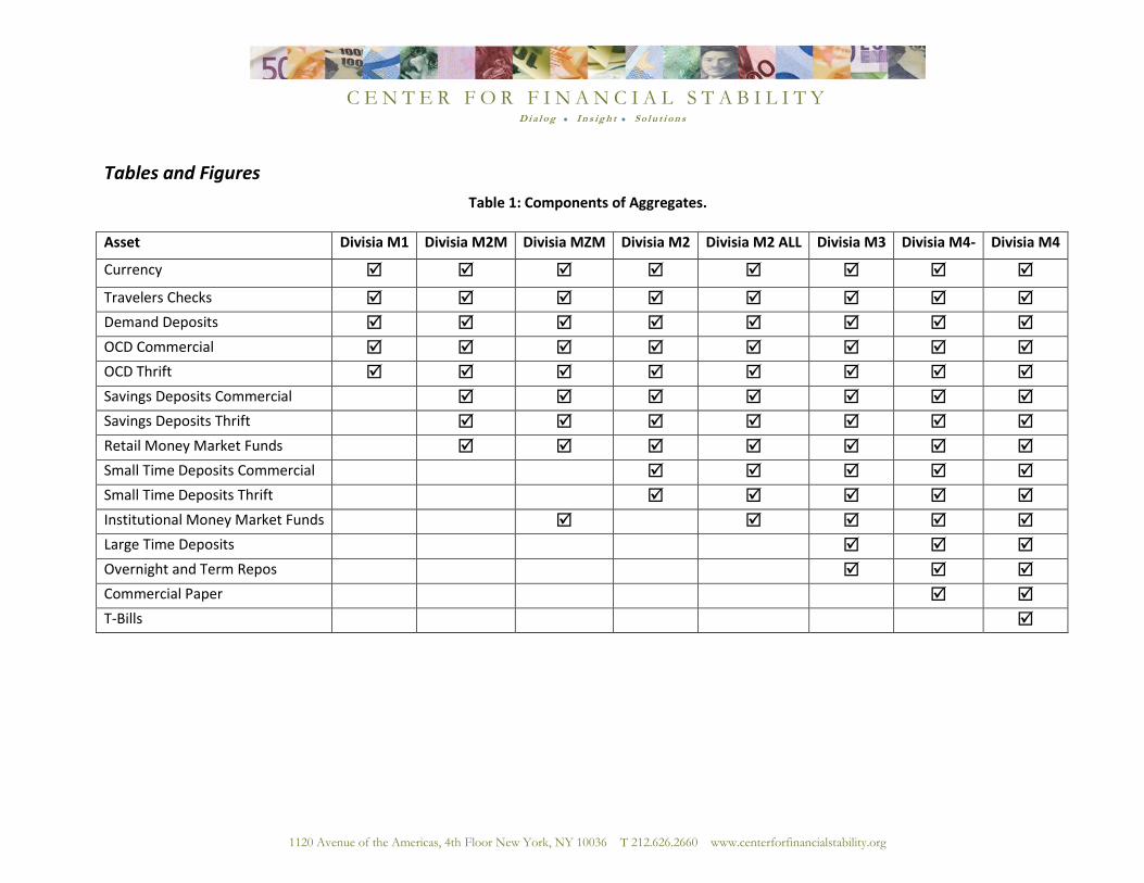
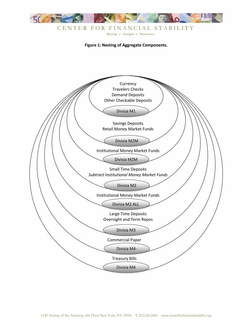
1 documents the component clusterings within each aggregation level, and Figure 1 displays the

resulting nesting of aggregates within aggregates, as the level of aggregation increases. When the

Federal Reserve discontinued publishing M3 and L, the Fed stopped providing the consolidated,

seasonally adjusted components. Also the Fed no longer provides the interest rates on the components.

With so much of the needed component quantity and interest-rate data no longer available from the

Federal Reserve, decisions about data sources needed in construction of the CFS aggregates have been

far from easy and sometimes required regression interpolation. This paper documents the decisions of

the CFS regarding United States data sources at the present time, with particular emphasis on Divisia M3

and M4.

The St. Louis Federal Reserve admirably initiated and maintains the five narrow Divisia monetary

aggregates for the US and calls them MSI (monetary services indexes), in accordance with the theory

and formulas derived by Barnett (1980). See Anderson and Jones (2011). But since the Federal Reserve

no longer provides its former broad aggregates, M3 and L, the CFS is now maintaining the broad

aggregates, Divisia M3 and Divisia M4, where M4 is similar to the Fed’s former broadest aggregate, L.

The CFS also is providing the narrow Divisia monetary aggregates, which are very similar to the St. Louis

Fed’s MSI aggregates. The primary distinction between the CFS’s and St. Louis Fed’s narrow Divisia aggregates is the measurement of the rate of return on capital (the benchmark rate), used within the

Divisia formula. The CFS’s and the St. Louis Fed’s narrow Divisia quantity aggregates can be expected

usually to behave similarly, although their dual user-cost price aggregates behave differently. The CFS is

providing the narrow Divisia aggregates as a hedge against possible future freezes of the St. Louis

Federal Reserve’s MSI database. Such a freeze occurred for the five years of the financial crisis and Great Recession, (March 2006-April 2011). The properly weighted broad aggregates, such as Divisia M3


-2-

and Divisia M4, are for most purposes the most informative. See Barnett (1982). The AMFM site focuses

primarily on the broad Divisia aggregates, which are provided solely by the CFS.

The Divisia aggregates in this CFS project are constructed for the purpose of making dependable

statistics available as painlessly as possible to the public. The most recent data are updated monthly,

will all details made public without subscription, at

http://www.centerforfinancialstability.org/amfm_data.php.

To that end and in accordance with the normal standards of science, we focus on the use of component

data available to the public. To assure replicability, we are providing all component data and are

withholding no sources or methodology or data from the public, as being proprietary to the CFS. That

task has proved to be much more complicated than anticipated. For example, national average bank

interest-rate data, previously collected and provided by the Federal Reserve, now are available only

from a private source requiring subscription fees. While much of the needed data are available within

the Federal Reserve by subscription to the private source, the Federal Reserve is currently not making

that data easily available to the public1. Our task has been further complicated by the discontinuance of

Federal Reserve collection of key components, such as repurchase agreements and bankers’ acceptances, previously available from the St. Louis Federal Reserve Bank website. The resources we

found for such hard-to find variables are provided in this paper, where available. Further complicating

our work is the fact that, even when component quantities are available for the former M3 and L

aggregates, those components often no longer are seasonally adjusted or consolidated. Without

seasonal adjustment, monthly growth rates contain seasonal noise; and without consolidation, simple-

sum accounting aggregation is vulnerable to distortions not consistent with reputable accounting

practices.

Data Sources

Constructing the Divisia monetary aggregates requires not only the quantities of monetary

components but also their interest rates. Following discontinuation of Federal Reserve collection of

some interest-rate and deposit-quantity data, we have had to find other public and private sources of

those data.2 While the Federal Reserve has agreements with the firms that now collect much of the

relevant data, the Fed does not presently provide them in their Statistical Surveys or through the St.

Louis Federal Reserve Bank’s online archive tool, FRED (Federal Reserve Economic Data). Table 2

documents our current components quantity and interest-rate data sources. The following paragraphs

also document prior sources used in producing the historical series, when sources were changing.

Much quantity (volume) data are available from the FRED website. From FRED we can find

many of the aggregates’ component levels, with the exception of large-denomination time deposits,

short-term treasury bills (T-bills), and overnight repurchase agreements (repos). Large time deposits can

be found in the Federal-Reserve-Board’s H.8 release, “Survey of Assets and Liabilities at Commercial

Banks.”3 While large time deposits were once readily available on FRED, current data from the H.8 are

no longer available there directly; one must access the data download program on the Federal-Reserve-

1 The authors would like to thank Richard G. Anderson at the St. Louis Federal Reserve Bank for providing much of

the needed data. The authors would also like to thank Steve Hanke, David Beckworth, and Peter Ireland for their

valuable input and suggestions. 2 See The Federal Reserve Discontinuation Memo on M3 and its Components.

3 http://www.federalreserve.gov/releases/h8/current/default.htm. See page 3, line 32 of the H.8 Survey for the

seasonally adjusted levels of large time deposits.


-3-

Board’s “Statistics and Historical Data” website. T-bills are available from the “Monthly Public

Statement of Debt” on the United States Treasury website4. Repos are available through the New York

Federal Reserve Bank’s “Primary Dealer Statistics” survey5; however, data before the beginning of this

survey had to be estimated using the now discontinued overnight and term RP level, provided by FRED

for commercial banks. Commercial paper levels are available on FRED only back to 2001; however, the

pre-2001 data can be found in the commercial paper section of the Federal Reserve Board Statistics site6

for monthly data and table L.208 of the Z.1 release, “Flow of Funds Survey,” provided by the Federal

Reserve Board.7 Quantity levels for the limited duration of “super negotiable orders of withdrawal” (super NOWs) and money-market deposit accounts (MMDA) were provided in the data set used by

Anderson and Jones (2011), and in previous issues of the Federal Reserve Bulletin.

Interest-rate data are more difficult to collect, as the Federal Reserve does not make them easily

available to the public or to researchers not on their staff. The Federal Reserve itself no longer tracks

the national averages of interest rates for bank products, nor does the St. Louis Fed currently provide

them on FRED. Federal Reserve Board staff are provided these data from outside sources, with whom

the Fed has contracts: (1) Bankrate.com, a company that keeps track of interest rates on deposit

accounts, mortgage loans, and credit-card rates; (2) ICAP, a London based firm, which provides interest-

rate data for overnight and term repurchase agreements; and (3) iMoney.net, which tracks interest

rates for money-market mutual funds.

Interest rates on checking, savings, money market-accounts, and certificates of deposit of

various maturities and levels (regular or “jumbo”) are collected and provided by Bankrate.com through two surveys: the weekly interest-rate roundup and the overnight daily internet survey. The weekly

“Bank Rate Monitor” survey is collected from the ten largest banks (five commercial and five thrift

institutions) in the 25 largest metropolitan areas of the United States. The result is a weekly sample of

250 of the largest banks by assets in the United States. The Bank Rate Monitor Survey is available for a

paid weekly subscription, which the Fed acquires and provides to its in-house researchers. The public

are not currently able to download the raw data to replicate the Fed’s research without a subscription. The second survey is a daily “Overnight Average,” provided freely on Bankrate.com’s website, or

available using Bloomberg for commercial banks and credit unions. The Overnight Average Survey is

conducted by collecting the interest rates offered for interest-checking accounts, MMDAs, jumbo CDs of

various terms, and mortgage and credit-card offer-rates available and advertised online. The overnight

CD data follow the Bank Rate Monitor rates fairly closely; however the MMDA and interest checking

rates for commercial banks are significantly higher and more volatile (as Bankrate.com warns on its

website explanation). The discrepancy is accounted for in the survey method: Bank Rate Monitor

4 http://www.treasurydirect.gov/govt/reports/pd/mspd/mspd.htm. There is no easily downloadable time series

data for the level of Treasury bills from the MSPD. The authors can provide that series on request to simplify other

efforts to replicate the data. 5 http://www.newyorkfed.org/xml/gsds_finance.html, under the tab “Financing.”

6 http: www.federalreserve.gov/releases/cp/volumnestats.htm. See the Data Download Program for

historical survey data. 7 http://www.federalreserve.gov/releases/z1/Current/. The data are taken on a quarterly basis in the Z.1 survey.


-4-

surveys the same ten largest banks each week in 25 cities, while the overnight average survey compiles

rates offered from various banks online. The overnight survey often collects only 30 to 40 daily-rate

offers from different banks. These online bank offers are generally higher than the average offers to

attract customers.

As of the writing of this paper, the Federal Reserve Bank of St. Louis has agreed to begin posting

the Bankrate.com data on the FRED website in spring of 2012. The St. Louis Fed has permission from

Bank Rate Monitor to make the average interest-rate data on various account types public, and we are

indebted to Richard Anderson at the St. Louis Fed for providing those interest-rate data to us in advance

of the anticipated public availability on FRED.

Money-market funds are collected by iMoneyNet. Federal Reserve researchers have access to

the data, which again are not currently provided by the Federal Reserve Board or FRED to the public. A

subscription is needed to acquire the data from iMoneyNet. We are indebted to Richard Anderson for

providing those data to us. But the public can acquire an alternative source available for free. The “7-

Day Average Rate” on money-market funds is available to the public on Bankrate.com through their

trend graph tool (which cites the source as iMoneyNet). There is no distinction there between retail or

institutional money-market funds, so one rate is used for both, when a separate institutional rate is not

available to the public. The separate retail and institutional money-market fund rates provided to us by

the St. Louis Fed were used until October of 2011. Starting in November of 2011, the alternative 7-Day

Average Rate available on Bankrate.com is used for both retail and institutional interest rates to permit

replication with data available to the public.

Repo rate data before 1997 had to be estimated by regression on T-Bill rates. After 1997 the

interest rate data came from the London firm ICAP, which takes an average of repo rates twice daily for

their I-Repo index, found on Bloomberg and in the Wall Street Journal.

Divisia M1 Aggregate

The Divisia M1 aggregate contains the most liquid monetary-asset components. Seasonally

adjusted levels of currency, travelers’ checks, and non-interest-bearing deposits are added and then

paired with a zero interest rate. Currency is the measure of cash available within the US economy

outside of the Federal Reserve. Currency quantities are available in the Fed’s H.6 Survey and on FRED. Travelers’ checks are freely available on FRED, as well. Like currency, traveler’s checks are assumed to

have a zero own rate or return.

While demand deposits can earn an implicit rate of return, we do not impute an implicit rate of

return to demand deposits. Anderson and Jones (2011) and Anderson, Jones, and Nesmith (1997)

investigated the possibility of assigning a non-zero own rate to demand deposits and proposed

alternative methods, originally suggested by Barnett and Spindt (1982), Farr and Johnson (1985), and

Thornton and Yue (1992). In these imputation procedures, household and business demand-deposits

are separated. As the relevant separated data are not readily available, the own rate of return for

demand deposits in the St. Louis Fed’s Divisia monetary aggregates is set to zero. The St. Louis Fed calls


-5-

its Divisia monetary aggregates “monetary services indexes” (MSI). While acknowledging that banks can

and do offer an implicit rate of return, especially to large depositors, we follow the same procedure as

the St. Louis Fed in foregoing the imputation of an implicit rate of return to demand deposits. The

reason is the lack of easily and openly-accessible data for such an imputation.

The levels of interest-bearing checking accounts (labeled as “other checkable deposits” or OCDs)

are also included in the aggregate. The interest rates on those accounts are available from either the

Bank Rate Monitor Survey or the Overnight Survey provided by Bankrate.com. Acquiring the own rate

of return for other checkable deposits before 1987 (the beginning of the Bank Rate Monitor survey) is

complex. From 1967 to 1973, OCDs are assumed to have a zero checking account yield, because of the

lack of data. From the period of 1974 to 1980, the own rates were the maximum allowed, which was

5%. The St. Louis Fed’s MSI index sets the own rate to be the minimum of either the 5% regulated limit

or the average of the most common interest rates reported on savings deposits in archived issues of the

Federal Reserve Bulletin. We simplify this period by adopting the 5% regulated limit for 1974 to 1980,

and the 5.25% maximum for the period from 1982 to 1983. Thrift-institution interest-checking accounts

are assumed to yield the same legal limits. In 1983, super NOW accounts were introduced, and the

super NOW interest rates are used for both other-checkable-deposits (OCDs) and the super NOW

accounts. The super NOW rates are available from the Federal Reserve Board in the Special

Supplementary Table of the Federal Reserve Bulletin back issues, accessible in the Federal Reserve

Archival System for Economic Research (FRASER) between 1983 and 1985. After January 1986, OCDs

include super NOW accounts. For the year of 1986, we use the average rate paid on NOW accounts as

provided by the Federal Reserve Board. We acquired that interest rate from the MSI component

spreadsheet provided to us by Richard Anderson for the paper Anderson and Jones (2011). After 1987

the rate or return on interest-bearing checking accounts is from the Bank Rate Monitor Survey.

Demand deposits and other-checkable-deposits (OCDs) are adjusted for retail sweeps. This

important adjustment procedure is described in the section below on “Sweeps”. Like the simple-sum

and MSI aggregates, the Divisia M1 monetary aggregate would be underestimated, if unadjusted post-

sweeps data were used for demand deposits and OCDs.

As is clear from the procedures described above, a clear and consistent data set on bank-

account interest rates is needed and would be useful, not only for construction of Divisia monetary

aggregates, which are far superior to the official simple-sum aggregates, but also for other research on

banking, finance, and monetary economics. We look forward to the anticipated FRED data availability,

planned to begin in the spring of 2012.

Divisia M2 Aggregate

The Divisia M2 aggregates include those components in the Divisia M1 aggregate, as well as

savings deposits, money-market deposit accounts, small-denomination time deposits, and retail money

funds. All of these component quantity levels come from the St. Louis Federal Reserve’s FRED database,

and the interest rates come from BankRate.com, with the exception of the national average of interest

rates for retail and institutional money market funds. The BankRate.com data are provided to us by


-6-

Richard Anderson at the St. Louis Federal Reserve under an agreement with BankRate.com to make the

component data public.

Levels of money-market deposit accounts (MMDA) on FRED come from the Federal Reserve

Board’s H.6 survey. Prior to 1991, MMDA and savings deposit quantities were treated as different

levels. MMDA level data began in 1982 and continue as separate levels until 1991. Savings deposits

without inclusion of MMDAs go back to 1967 and continue to 1991 as well. Since 1991, MMDA and

savings-deposits data have been merged and are counted as one item.

Interest rates from MMDA and savings accounts were treated separately up to October 1991.

Following Anderson, Jones, and Nesmith (1997), we used the maximum legally-available rate until 1983

for savings and MMDA accounts, with thrift institutions’ maximum rate being the commercial-bank rate

increased by 25 to 75 basis points, depending on the time period. From 1983 to 1991, MMDA levels are

paired with average interest rates reported by the Federal Reserve Board in the data set provided by the

St. Louis Fed for the paper, Anderson and Jones (2011). From 1986 to 1991, that data set is also used to

acquire the average monthly interest-rate paid on savings deposits. After 1987, MMDA and savings

levels are combined and coupled with the interest rates on MMDAs, provided by Richard Anderson at

the St. Louis Fed from the weekly Bank Rate Monitor survey.

Small denomination time deposit levels are also readily available on FRED from the H.6 survey of

the Federal Reserve Board. Seasonally adjusted levels are consistently taken and posted from 1967 to

the current period. These deposit denominations are less than $100,000, unlike their large

denomination or “jumbo” counterparts measured in the Board’s H.8 Survey.

Small denomination time deposits require a similar mix of data series. From 1967 to September

1983, the 6-Month CD interest rate for commercial banks is used as the own rate for small time

deposits. The thrift rate is computed by adding 25 basis points to the commercial bank interest rate.

Between October 1983 and August 1991, the own rate is computed to be the average rate of return paid

by commercial banks and thrift institutions for balances of less than $100,000 with maturities of 92 to

182 days. After August 1991, the 6-Month CD rate for commercial bank and thrift institutions is used

from the Bank Rate Monitor survey, as provided by the St. Louis Federal Reserve Bank (Richard

Anderson).

The Federal Reserve still posts money-market funds on FRED, as they contribute heavily to the

simple-sum measures of M2 and MZM. The seasonally adjusted levels posted on FRED come from the

Board’s H.6 Money Stock Measures survey, and stretch back consistently to our 1967 starting point for

both retail and institutional money-market funds. Retail money-market funds are those offered

primarily to individual investors and have a low minimum investment quantity. Institutional money

funds are designed with businesses in mind, and have high investment requirements, but also provide

higher interest-rate return than retail money-market funds. For some businesses, the institutional

money-market funds are linked to a company’s demand deposits or other-checkable-deposit (OCD)

accounts, with funds being “swept” into money-market funds at the end of the business day, when

demand deposit and OCD accounts are not in use. This “Commercial Sweeping” is covered in more


-7-

detail in the “Sweeps” section below. It should be noted that any M2 aggregates, Divisia or simple-sum,

will be underreported, unless they include the institutional money-market funds that include these

sweeps.

From 1974 to 1987, there is only one rate to match with both retail and institutional money-

market funds. These data are provided by the St. Louis Fed in Anderson and Jones’s (2011) MSI

component data, and are cited in that paper as unpublished data obtained from the Federal Reserve.

The separate retail and institutional money-market fund interest rate data from 1987 to 2011 also come

from Anderson and Jones (2011), which cites the source as an unpublished Federal Reserve data set

from iMoney.net. The money-market fund rates have not yet been posted on FRED, and are otherwise

only available through a subscription to iMoney.net. We are indebted to Richard Anderson for providing

those data to us. From November 2011 to the present we use the 7-Day Average Money Market Fund

Rate available on Bankrate.com for both retail and institutional money-market funds. The Bankrate.com

source is easily accessible and available to anyone with an internet browser using the graphing tool.

Each Divisia M2-variant aggregate includes or excludes certain components, in parallel with the

corresponding simple-sum aggregates commonly used by the Fed. Divisia M2M incorporates savings

deposits, MMDA, and retail money-market funds, but not small time deposits (small-denomination CDs).

Divisia MZM includes the components of Divisia M2M, along with institutional money-market funds.

Divisia M2 omits institutional money-market funds, but incorporates small-denomination time-deposit

levels and rates. Divisia M2-ALL reincorporates institutional money-market-fund data into the

components of Divisia M2.

The Divisia M2 aggregates are designed to follow closely the structure of simple-sum and MSI

variants of M2. Further empirical testing on how to cluster the Divisia M2 aggregates’ components

would be useful, but is left to future research.

Divisia M3, M4-, and M4 Aggregates

The Divisia M4 aggregates (Divisia M4- and Divisia M4) are derived by incorporating into Divisia

M2 the levels and rates of return on the primary, negotiable, money-market securities, including

commercial paper, large-denomination time deposits, overnight repurchase agreements (repos), and

short term treasury bills (T-bills). Being highly liquid, these primary securities contribute to the

economy’s flow of monetary services, but not to the same degree as currency and checkable deposits. These aggregates are meant to substitute for the now discontinued Federal-Reserve simple-sum L

aggregate, but with proper aggregation-theoretic weighting of the components, as opposed to the

former simple-sum aggregation, which produced a greatly distorted measure of the economy’s liquidity, by weighting all components the same as legal means of payment. Divisia M4- removes T-bills from

Divisia M4, for use in applications requiring separation of monetary from fiscal policy effects. Divisia M4

includes T-bill rates, to round out the most general Divisia aggregate within this project. Acquiring the

necessary data to compute M4 was challenging, since many of the components of L are no longer

provided by the Federal Reserve Board, especially in seasonally-adjusted consolidated form.


-8-

The interest rates for commercial paper are available on FRED and also on the Board’s H.15

Survey of Selected Interest Rates. From 1967 to 1996, the interest rate we use on commercial paper is

the interest rate on “Finance Paper Placed Directly” with a three month maturity. We use that rate,

since it is the only three-month-maturity rate available for “Financial or Nonfinancial Commercial Paper”

during that time period, and for overlapping periods tracks the AA financial paper rate well. The rate for

finance paper is available through the Federal Reserve Board Statistics H.15 Selected Interest Rates

survey, using the data download program8. From 1997 to the present, the “AA Three Month Financial

Commercial Paper” rate is used as the own rate of interest and is available on FRED. The rate of return

on financial commercial paper is used, since commercial paper issued by financial companies is the bulk

of commercial paper issued. Commercial paper with 3-month maturity was the focus, since 3-months is

the middle term of the maturities tracked by the Fed. The Fed provides data on maturities between one

and six months.

Commercial paper quantity data are readily accessible on the Federal Reserve Board website

and on FRED. Quarterly data from the Z.1 Flow of Funds Survey had to be used before 1991 as monthly

asset level data on commercial paper was unavailable. These figures are available in L.208 Table. After

1991, asset levels can be found in two available surveys on the commercial paper site of the Board of

Governors. The first survey is the “old structure” survey, starting in January of 1991 and including

monthly levels. In 2006, several changes were incorporated into the commercial paper calculations9,

and the Federal Reserve Board had to begin a different “new structure” series that continues today. The new series data begin in January 2001 and continue to the present. To link these series, a regression

was run on the overlapping periods (January 2001 to March 2006) of the old and new survey, and past

values of the “new structure” were estimated from the “old structure.”

The own rate of return on large-denomination time deposits is the 6-Month Secondary

Certificate of Deposit Rate available on FRED. This follows from the method of Anderson and Jones

(2011) in calculating the MSI for M3 components before their discontinuance. Fortunately the interest

rates for CDs are still easily available on FRED. On the other hand, levels for large-denomination time

deposits were discontinued in FRED and are accessible in the Federal Reserve Board’s H.8 “Survey of

Assets and Liabilities of Commercial Banks.”

The levels of non-seasonally adjusted T-bills were compiled into a data sheet from the “Monthly

Public Statement of Debt,” provided by the United States Treasury Department. The levels include

those T-bills held by the public plus the amount held by intergovernmental agencies. There are no large

time-series data available for download for levels of T-bills, but the compilation of data we used is

available upon request.10 The own rate of return for T-bills is the secondary-market rate for the 3-

month maturity T-bill, available on FRED back to 1967. These rates originally come from the Board’s H.15 “Survey of Selected Interest Rates” and can be accessed on the Federal Reserve Board website as

well.

8 http://www.federalreserve.gov/datadownload/Build.aspx?rel=H15.

9 A description of these changes can be found here: http://www.federalreserve.gov/releases/cp/about.htm.

10 Otherwise a potential replicator will have to wade through monthly scanned documents back to 1967.


-9-

Levels of overnight and term repos are available through the New York Federal Reserve Bank’s Primary Dealer Statistics on the New York Fed’s website. However those data only stretch back to

November of 2001. FRED contains levels of overnight and term repos that were used in the now

discontinued M3 aggregate; however, those data only extend from 1970 to 2006. The two data series

are also not equal. The New York Fed repos are those processed daily between the “primary dealers” (banks, security dealers) and the Fed, and are very large. The repos used in the former official M3

aggregate, available on FRED, were those issued by commercial and thrift banks to customers. Those

quantities are relatively low. We chose to estimate the 1970 to 2001 values of the New York repos using

the estimated coefficient of a regression of the New York Fed values on the FRED values for the

overlapping time period of 2001 to 2006. After 2001, the actual values from the New York Fed

overnight and term repos are used, up to the most current period.

The rate data are provided by the London-based money broker, ICAP. ICAP’s I-Repo index is an

average of interest rates on repurchase agreements taken once at 12:00 PM EST (“AM Rate”) and 6:00 PM EST (“PM Rate”). For repo levels from 1997 to the present, a time series of repo rates was provided

by Datastream Navigator, and correspond to the PM rate taken. These values are available using the

Bloomberg11 website, and searching for the “I-Repo Index”. The I-Repo Index uses the morning value of

repo interest rates and corresponds to the AM rate. The AM I-Repo rate can also be found in the Wall

Street Journal12. Repo rate data before 1997 are unavailable, so the repo rates were estimated in

overlapping time periods of the Datastream series by regression on T-Bill rates (from FRED), which were

found to be closer than other interest rates to the repo rates. Using the estimated regression

coefficient, the repo rates were estimated back to 1970, using the available T-bill rates.

The Divisia M3 aggregate contains a similar set of components to the discontinued simple-sum

aggregate, produced by the Federal Reserve before 2006. Along with the components of M2-ALL13,

Divisia M3 includes large time deposits and overnight and term repurchase agreements.

The Divisia M4 aggregates are the broadest available monetary aggregates and are supplied only

by the CFS in its AMFM program. They reflect the spirit of the monetary aggregate, L, formerly available

from the Federal Reserve, and the Divisia M4 aggregates capture most of L’s former components. A

noted absence is bankers’ acceptances. The interest rates for bankers’ acceptances, according to the

Board’s H.15 “Survey Historical Data,” were available through the firm, Telerate, which provided the Fed

with those rates until June, 2000. A search for the company shows it was bought by Thomson-Reuters.

Telerate became “Moneyline Telerate, Inc.” in 2001, and does not seem to provide the bankers’ acceptance rates anywhere. When searching for bankers’ acceptance levels, we learned, from the

description of the L.208 Open Market Paper table of the Z.1 Survey, that Bankers’ Acceptance levels are

no longer differentiated from commercial paper. Any levels of bankers’ acceptances are included in the

11

http://www.bloomberg.com/apps/quote?ticker=IREPUSOA:IND 12

http://online.wsj.com/mdc/public/page/2_3020-moneyrate.html 13

Institutional money-market funds used to be a part of simple-sum M3, and are not included in the “old” M2 definition. Currently they are used in MZM and M2-ALL.


-10-

commercial paper levels, and coupled with a commercial paper rate, since the two are no longer

separated.14

Sweeps

It is well known that retail sweeps programs have a decreasing effect on the quantities of

components in M1 (both simple-sum and Divisia). Retail sweeps occur when banks move money on

their accounting books from non-interest bearing or low-interest-bearing checking accounts (demand

deposits or OCDs) to savings and MMDA accounts, which are not subject to reserve requirements. Such

swept funds are not included within official M1. Without an adjustment for the funds being “swept” from Divisia M1 components to Divisia M2 components, Divisia M1 will be biased downwards. It should

be observed that such sweeps are serviced as checking accounts, so the “sweeps” are little more than an accounting measure, unrelated to the economics of the swept funds’ services, which belong in M1. For

narrow monetary aggregates, a corrective sweep adjustment is necessary to avoid economic distortion

of the services being measured.

To account for bookkeeping sweeps from demand deposit and OCD accounts into savings and

MMDA deposit accounts, the total amount of estimated sweeps is taken from the St. Louis Federal

Reserve website, under the category of “cumulative sum of newly initiated retail sweeps”15. The sweeps

levels are allocated to demand deposits and OCDs, based on the shares of total demand deposits and

OCDs in commercial and thrift accounts. The amounts added to demand deposits and OCDs are then

subtracted from the savings deposits, based on the total shares of savings deposits in commercial and

thrift institutions.

The sweeps data on the St. Louis Federal Reserve Bank website measure the amount of new

sweeps programs initiated in MMDA accounts. These new programs are then summed over time to get

the cumulative amount of sweeps. This cumulative figure is the amount used in our adjustment

procedure, since that figure is a simple, available measure of total sweeps in the system. But this figure

underreports the amount of sweeps, since banks have no obligation to report the level of sweeps they

initiate.

To maintain a current monthly release, the previous month’s sweeps values are used. For

example, the January 2011 sweeps level is used for the February 2011 Divisia calculation. The lag value

is chosen as the proxy (martingale forecast) for the current month’s sweeps, since the sweeps levels are not available to the public until nearly two months after the corresponding month. While the value is

available internally to Federal Reserve Board researchers in the proper month, contemporaneous

sweeps data are not posted on the St. Louis Fed’s website until the following month. To assure

replicability by the public, we are avoiding use of internal Federal Reserve data prior to availability to the

public. We recalculate the prior month’s Divisia indexes, as soon that month’s sweeps become available to the public. As a result, only the current months aggregates depend upon lagged sweeps. In an

14

http://www.federalreserve.gov/apps/fof/DisplayTable.aspx?t=l.208. See “description” for note on bankers’ acceptances. 15

http://research.stlouisfed.org/aggreg/swdata.html.


-11-

experiment, the Divisia indexes were calculated using both the current month (for those months

available) and the lagged month, and we found no significant differences between the two series. As a

result, the recursive recalculations of the prior month’s aggregates produce negligible changes to the

historical data.

Let DD be demand deposits, DDS be sweeps-adjusted demand deposits, OCDC be other

checkable deposits at commercial banks (interest bearing checking accounts), OCDCS be the sweep-

adjusted OCDC, OCDT be other checkable deposits at thrift institutions, OCDTS be the sweeps-adjusted

OCDT, and CD be the level of cumulative sweeps provided by FRED. Then the adjusted levels are as

follows.

Similarly, the process adjusting savings deposits for sweeps is as follows, where SAVC are savings

deposits at commercial banks, SAVCS are the sweeps adjusted-level of SAVC, SAVT are savings at thrift

institutions, and SAVTS are the sweeps-adjusted level of SAVT:

Furthermore, commercial sweeps programs produce further understatement of narrow

monetary aggregates. Jones, Dutowsky, and Elger (2005) have noted a significant increase in demand-

deposit amounts “swept” into institutional money-market funds and other financial instruments, since

the 1990s. Unlike retail sweeps, customers tend to be informed of these commercial sweeps, when

banks move funds from accessible demand deposits to a linked investment account. Since commercial

sweeps are more than just accounting devices, customers share in the earnings from those sweeps.

Jones et al. (2005) provide a method for adjusting the narrow monetary aggregates to account for

commercial sweeps by moving amounts out of institutional money-market funds and back into demand

deposits and other checkable deposits. However, this adjustment would not account for those

commercial sweeps in unlinked investment accounts. There are no data for those sweeps or for those

linked to financial instruments other than money-market funds. The problem is minimized by broad

monetary aggregates, such as the Divisia M4 aggregates. Because of lack of data, we have not

compensated our narrow Divisia monetary aggregates for commercial sweeps, and we do recommend

the use of broad aggregates to offset the problem. But even without this problem, there are many good


-12-

reasons to prefer a properly weighted broad aggregate to a narrow aggregate, which arbitrarily assigns a

weight of zero to some liquid assets, providing monetary services to the economy.

The Benchmark Rate

The user-cost price of the services of a monetary asset depends upon the interest foregone to

consumer the services of the asset. The interest foregone depends upon the interest paid by the asset

and the higher expected rate of return on the benchmark rate, defined to be the rate of return on pure

investment capital, providing no monetary services. To determine the benchmark rate, which cannot be

less than the own yield on a monetary asset providing monetary services, we compute the upper

envelope over the own rates of return on the components of our broadest monetary aggregate, M4.

We do not constrain the upper envelope to the components of the St. Louis Federal Reserve’s narrower M2-ALL aggregate. The benchmark rate can never be less than the upper envelope level at any period

of time. But the benchmark rate normally should exceed that upper envelope, since the benchmark rate

is a proxy for a shadow rate having no liquidity, being the theoretical rate of return on pure capital

producing no services other than investment yield. In addition, such pure capital investment return is

normally taxed at a lower rate than the rate of interest on monetary asset accounts. For those reasons,

we include within the computation of our upper-envelope the “Weighted Average Effective Loan Rate, Low Risk, 31 to 365 Days, All Commercial Banks” (C&I Loan Rate) from FRED. We are indebted to Akiva

Offenbacher at the Bank of Israel for this suggestion, which also is used in computation of the Bank of

Israel’s new Divisia monetary aggregates.

The low-risk bank-loan rate was chosen to keep within a “risk neutral” setting required by the derivation of the Divisia monetary aggregate formula we are using. See Barnett (1980). While we have

available the risk-adjusted formula to account for risk aversion, we are not currently using that

extension. The C&I loan rates come from the E.2 “Survey of Terms of Business Lending,” provided by

the Federal Reserve Board. The secondary negotiable CD loan rate and the Eurodollar deposit rate were

considered for comparison. The three month secondary negotiable CD rate and the six month

Eurodollar deposit rate is available on FRED and in the Board’s, H.15 ”Survey of Selected Interest Rates.” But we decided upon the C&I loan rate, which acts as an upper limit to the interest rate a bank will offer

on any deposit category. A bank will not pay out to its depositors more than it earns in interest on the

short-term loans it makes. The low-risk C&I loan rate is most often the maximum of the interest rates in

the upper envelope, as expected. The C&I loan rates are available only as quarterly data. As a result,

that rate in our benchmark-rate computation is used for all three months in the quarter. The Bank of

Israel has that rate monthly.

Since the C&I loan rates is not available before 1997, just the upper envelope of the M4

component interest rates The lack of C&I loan rates leads in some periods to commercial financial paper

having a zero user-cost level, since its rate is the highest for those periods. For the benchmark rate,

before 1997, 100 basis points are added to keep user costs from becoming zero, following a

methodology by Anderson and Jones (2011). Once C&I loan rates are introduced, the addition of 100

basis points is no longer necessary, as C&I loan rates are always greater than those rates banks offer to

pay on the component aggregates.


-13-

Seasonal Adjustment and Consolidation

Some components of M3, M4-, and M4 are no longer available in seasonally adjusted or

consolidated form. Specifically the levels of short term treasury bills and overnight repurchase

agreements are not seasonally adjusted by their respective sources. We employed the commonly used

X-12 ARIMA (autoregressive integrated moving average) procedure to seasonally adjust the data, as is

done by the United States Census Bureau16.

A detailed description of the methods and theory of X-12 ARIMA can be found at the US Census

Bureau website17, and its advantages are outlined in a study by Thorp (2004), defending the Bank of

England’s switch to using the X-12 ARIMA seasonal adjustment for its monetary components. A further

study of X-12 ARIMA by the European Central Bank (2000) details its use in measuring the money supply

of the European Union in the exhaustive Seasonal Adjustment of Monetary Aggregates and HICP for the

Euro Area. Our analysis of the data after seasonally adjusting T-bills and Repos produced no reason to

use an alternative method to the mainstream.

The unadjusted levels are readily available in the sources described in this paper. To access non-

seasonally adjusted levels of T-bills and repurchase agreements, one need only visit the Monthly

Statement of Public Debt on the US Treasury website, and the New York Federal Reserve Bank’s Primary Dealer Survey. With those unadjusted resources, any seasonal adjustment method could be applied.

Alternatively, to avoid seasonality distortions in non-seasonally adjusted broad aggregates, one could

calculate only year-over-year growth rates18. All components used in the narrower Divisia aggregates

(M1 and the M2 family) are seasonally adjusted. However, to properly measure the broader aggregates

that include t-bills and repos, either seasonal adjustment must be performed or alternatively only year-

over-year growth rates should be used to avoid seasonality problems.

On the CFS’s Advances in Monetary and Financial Measurement website, we display the seasonally adjusted year-over-year growth rates. The year-over-year method is preferred primarily

because of the lower volatility of the growth rates. If monthly growth rates are desired, the monthly

levels of the Divisia aggregates can be used to compute the month-over-month growth rate, since all of

our quantity data are seasonally adjusted.

Consolidation is an accounting convention relevant when numbers are added up. For example,

consolidation is necessary to net out the overlap between money-market funds, which include

16

The X-12 ARIMA process is also used by the Federal Reserve Board as in Pierce (1983), the Bank of England as

outlined in Thorp (2003), and the European Central Bank (2000) in Seasonal Adjustment of the Monetary

Aggregates. 17

http://www.census.gov/srd/www/x12a/. 18

There are two possible methods of computing year-over-year Divisia growth rates: (1) the Divisia weights could

be based upon the average of the components’ expenditure shares between the contemporaneous observation and the one-year lagged observation, or (2) the Divisia index could be chained monthly to produce the level index

series, and then the year-over-year growth rates could be computed from the levels series, as advocated by

Diewert (1999). We use the latter procedure, since that procedure more closely approaches the continuous-time

share weighting and hence produces a higher quality index. We use the year-over-year convention only to produce

growth rates. We do not use that approach to produce the levels series.


-14-

negotiable CDs in their portfolios, and the total market quantities of negotiable CDs. Without

consolidation, adding up money-market funds and negotiable CD primary securities would produce

double counting. But consolidation is irrelevant to Divisia monetary aggregation, which is based on

economic theory and requires market data, not consolidated accounting data. Since we provide no

simple-sum monetary aggregates at any level of aggregation, the lack of consolidated data is not a

problem for the CFS monetary aggregates.

Entry and Exit of Assets to and from the Aggregates

Our database extends back in time to 1967. Between 1967 and now, there have been entries

and exits of assets from the database. For example, super-Now and MMDA accounts have not been in

existence throughout the entire time span. In index number theory, a literature exists on how to deal

with such innovations. Crossing the boundary between existence and nonexistence of an asset can

severely damage an index number, if done incorrectly. For example, if the Divisia index is used to cross

that innovation boundary, the index will explode to plus or minus infinity. The Divisia index uses log

changes for growth rates. The quantity growth rate of an asset from a period when an asset does not

exist to the next period, when the asset does exist, is infinity. Conversely the quantity growth rate of an

asset from a period when an asset does exist to a period when the asset no longer exists is minus

infinity.

To deal with this problem, the formal procedure often advocated in the literature is to impute a

reservation price to the asset for the period when the asset does not exist and switch to the Fisher ideal

index to cross the innovation boundary. We use a different procedure. We do not include an asset in

the aggregate during such a transition period. When a new asset appears, we do not enter it into the

aggregate until the asset has been in existence for two successive periods. We then use the growth rate

from the innovation period to the next period to introduce the asset into the aggregate. Analogously,

when an asset disappears from existence, our last entry for that asset is for the growth rate from the

prior period to the last period of existence. We never cross the boundary to use the growth rate

between a zero entry and a positive entry in either direction.

Our procedure produces no discontinuities. The Divisia index formula is used to produce the

growth rate of the aggregate. The growth rates are recursively cumulated to derive the level series,

starting from 100. The growth rate during a transition period is computed from the Divisa growth rate

of those components not subject to transition during that period. In contrast, simple-sum aggregation

introduces a discrete jump into or out of the total, when an asset enters or leaves. Such transitions

often result from movement of funds from one discontinued category into another, or from a change in

availability of relevant component data. As a result, the resulting simple-sum discontinuous jumps often

are severely misleading. Within monetary aggregates, such transitions rarely reflect a technological

innovation creating a “new good,” and rarely imply invention of a new source of legal means of

payment, appropriately weighted the same as cash, as in the simple-sum aggregates. Our procedure

produces smooth transitions, with the transition asset’s growth not permitted to influence the

aggregate’s growth rate during the transition period.


-15-

User Cost and Interest Rate Aggregation

The literature relevant to interest rate aggregation is different from the literature relevant to

user-cost aggregation. User-cost aggregation is a form of price aggregation, which is a subject of

economic aggregation and index-number theory. User cost measures foregone interest and thereby the

opportunity-cost price of consuming the non-investment services of an asset, such as liquidity and

means of payment. In contrast, interest rate aggregates, rather than measuring interest foregone,

measure interest received as return on investment. Interest rate aggregation is based on elementary

accounting principles, not on economic theory.

We use Fisher’s factor reversal test formula to compute user-cost price aggregates. By that

method, the user cost aggregate over a collection of assets is equal to the user-cost evaluated

expenditure on the component assets divided by the aggregation-theoretic aggregate over the

component quantities. More formally, suppose the user-cost prices of the n monetary assets, m, are, π,

so the expenditure on the services of the assets is 1

n

i ii

m , and suppose M(m) is the aggregation-

theoretic quantity aggregate over m. Then the user cost aggregate is1

( ) ( )n

i ii

m M

π m , so that

1( ) ( )

n

i ii

M m

π m . We use the discrete time Divisia index to compute the quantity aggregates, as

originally derived by Barnett (1980). The user-cost aggregate produced from factor reversal is the dual

to the quantity aggregate. Since the Divisia index formula is not self-dual, the user-cost aggregate is not

itself a Divisia index. The derivation of the formula for the user cost prices, π, can be found in Barnett

(1980).

The procedure for computing interest rate aggregates, being based on accounting principles, is

considerably more elementary than the procedure for computing user cost aggregates. The interest

rate aggregate for a portfolio of monetary assets is the single interest rate at which the portfolio would

yield the same investment return as the actual return on the portfolio having separate rates of return on

each component asset. More formally, suppose a portfolio of n monetary assets, m, is receiving interest

rates, r, so the return on the investment is 1

n

i ii

r m . Then r(r) is the aggregate interest rate yield on

the portfolio, if 1 1

( )n n

i i ii i

r m r m

r for any interest rates r. Solving for r(r), we immediately find that

1 1( )

n n

i i ii i

r r m m

r , which is the quantity weighted average of the component interest rates. We

use that accounting formula to compute the interest rate aggregates corresponding to each monetary

aggregate.

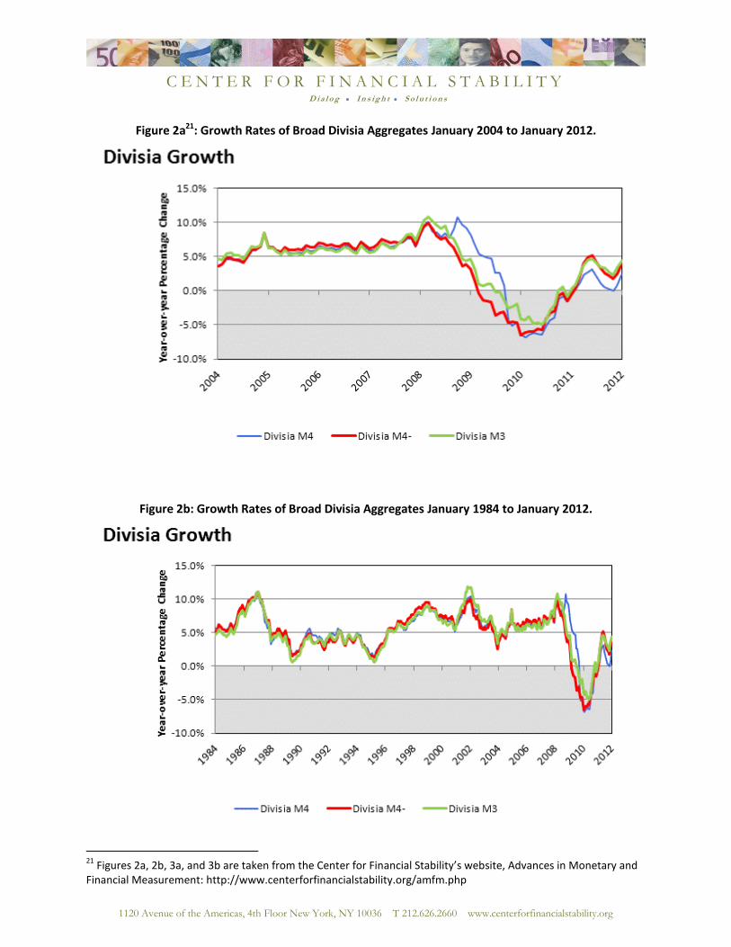
Conclusion

The purpose of this paper is to document the sources and procedures used in producing the

new CFS Divisia monetary aggregates database. Other papers by other authors are already using that

data in policy-relevant research, such as Serletis and Gogas (2012) and Belongia and Ireland (2012). But

the policy relevance is immediately evident from inspection of Figures 2a, 2b, 3a, and 3b below. In

particular the explanatory power relative to the recent financial crisis and subsequent Great Recession is


-16-

clear, as is the contrary evidence about the widely expected future inflation, as has been observed by

Hanke (2011a,b). In addition, the need for these data are heavily documented and motivated in Barnett

(2012). For these reasons, we feel that full disclosure of the data sources and methodology are

important.



Tables and Figures

Table 1: Components of Aggregates.

Asset Divisia M1 Divisia M2M Divisia MZM Divisia M2 Divisia M2 ALL Divisia M3 Divisia M4- Divisia M4

Currency

Travelers Checks

Demand Deposits

OCD Commercial

OCD Thrift

Savings Deposits Commercial

Savings Deposits Thrift

Retail Money Market Funds

Small Time Deposits Commercial

Small Time Deposits Thrift

Institutional Money Market Funds

Large Time Deposits

Overnight and Term Repos

Commercial Paper

T-Bills



Figure 1: Nesting of Aggregate Components.

Currency

Travelers Checks

Demand Deposits

Other Checkable Deposits

Savings Deposits

Retail Money Market Funds


Small Time Deposits

Subtract Institutional Money Market Funds


Large Time Deposits

Overnight and Term Repos

Commercial Paper

Treasury Bills

Divisia M2 ALL

Divisia M3

Divisia M4-

Divisia M4

Divisia M2

Divisia MZM

Divisia M2M

Divisia M1



Table 2: Current Data Sources.

Asset Rate Rate Source Level Source

Currency 0% NA FRED / H.6

Travelers Checks 0% NA FRED / H.6

Demand Deposits 0% NA FRED / H.6

OCD Commercial Interest Checking Commercial Bank Rate Monitor FRED / H.6

OCD Thrift Interest Checking Thrift Bank Rate Monitor FRED / H.6

Savings Deposits Commercial MMA Rate Commercial Bank Rate Monitor FRED / H.6

Savings Deposits Thrift MMA Rate Thrift Bank Rate Monitor FRED / H.6

Small Time Deposits Commercial 6-Month CD Rate Commercial Bank Rate Monitor FRED / H.6

Small Time Deposits Thrift 6-Month CD Rate Thrift Bank Rate Monitor FRED / H.6

Retail Money Funds Retail Money Market Funds Rate iMoneyNet19 FRED / H.6

Institutional Money Funds Institutional Money Market Funds Rate iMoneyNet20 FRED / H.6

Commercial Paper 3-Month AA Financial Commercial Paper Rate FRED / H.15 FRED / Commercial Paper Survey

Large Time Deposits 6-Month Secondary CD Rate FRED / H.15 FRED / H.8

Overnight and Term Repurchases I-Repo Index Rate ICAP (Bloomberg) Primary Dealer Statistics, NY Fed.

Treasury Bills 3-Month T-Bill Secondary Market Rate FRED / H.15 Monthly Survey of Public Debt.

Eurodollar Deposits Eurodollar Deposit Rate FRED / H.15 NA

Negotiable CD Rate 3-Month Secondary CD Rate FRED / H.15 NA

Commercial and Industrial Loans Weighted Average Effective Loan Rate, Low Risk,

31 to 365 Days, All Commercial Banks (EEMLNQ).

FRED / E.2 NA

19

Unpublished source of data used by the Federal Reserve. As a substitute starting in November 2011, we use the “iMoneyNet 7-Day Average Yield” found in the Graph Rate Trend Tool on bankrate.com (http://www.bankrate.com/funnel/graph/). 20

Unpublished source of data used by the Federal Reserve. As a substitute starting in November 2011, we use the “iMoneyNet 7-Day Average Yield” found in the Graph Rate Trend Tool on bankrate.com (http://www.bankrate.com/funnel/graph/).



Figure 2a21

: Growth Rates of Broad Divisia Aggregates January 2004 to January 2012.

Figure 2b: Growth Rates of Broad Divisia Aggregates January 1984 to January 2012.

21

Figures 2a, 2b, 3a, and 3b are taken from the Center for Financial Stability’s website, Advances in Monetary and Financial Measurement: http://www.centerforfinancialstability.org/amfm.php


-2-

Figure 3a: Implied Interest Rate of the Divisia Aggregate January 2004 to January 2012.

Figure 3b: Implied Interest Rate of the Divisia Aggregate January 1984 to January 2012.



Appendix: Regression Estimates for Broad-Aggregate Component Levels and Rates.

For the broad-aggregate components not all data were available from a single source survey, or

in some cases were not available at all for historical values. These levels and interest rates are

estimated to fit with the current resources. In all cases a simple linear regression without a constant

was used to approximate the past values. These estimations are used in the case of component levels

for large denomination time deposits, levels of commercial paper, and levels and rates of repurchase

agreements.

Because of the lack of data or the use of two distinct surveys for repo asset levels and interest

rates, the past values of the components are estimated using a growth rate method of back calculation.

A simple linear regression estimate was taken as well, but the splice produced large jumps at the point

in time the series were linked22. To avoid this jump, the growth rate method is used for the levels of

repos instead. For the linear regression estimate, the values of the estimated survey are about 2.97

times those of the original, while the values for the growth rate method are 2.51 times the original

levels. is the level of repos from the New York Fed’s Primary Dealer Statistics survey, and is the monthly overnight and term RPs for commercial banks, available but discontinued on

FRED. As previously mentioned, these two surveys are different, since takes values for all

primary dealers (banks, securities), while is described in FRED as only surveying commercial bank

deals. The monthly growth rates for each series were calculated, and , where D is

the percentage growth rate operator. The growth rates from the FRED series are preserved for the

months before October 2001, and then used to back calculate the levels from the initial level of the

Primary Dealer Survey. For T, the time of the splice (October 2001), the initial Primary Dealer Survey is

used to estimate the last value for repo levels available on FRED: ̂ ⁄ .

For all the preceding time periods, , the levels were estimated following the back

calculation pattern and the available levels from the FRED survey: ̂ ⁄ .

The values for interest rates of repos were not available before 1995, and there was no comparable

survey of repo rates from which to estimate. The available repo rates after 1995 were compared

graphically to other interest rates, and the T-Bill rate was found to be the closest approximation and

most useful, since it is available back to 1967 without any significant splices or changes of survey.

Another linear regression without a constant was taken to determine the coefficient for the past values

of the I-Repo interest rate index:

22

The linear regression without a constant estimate follows the procedures outlined later in this paper for the

estimation of the interest rate levels of repurchase agreements, the levels of commercial paper, and large time

deposits. The coefficient of estimation was estimated at 2.9723, using the overlapping survey period of October

2001 to March of 2006, and the survey switch occurred in October 2001.


-2-

,

where is the IREPO Index, is the coefficient of the interest rate, and is the 3-month

Treasury bill secondary market (monthly) rate from FRED. For the overlapping period from November

1996 to December 2011, was estimated, and the past values of the repo interest rate were then

determined by: ̂ ̂ .

In addition to estimating repo levels and rates, we spliced the levels for large denomination time

deposits and commercial paper to compensate for their collection by two different surveys. The splice

again uses a simple linear regression, and estimates the coefficient of the levels between the two

surveys without intercept. For commercial paper, both asset level surveys are available from the

Federal Reserve Board Statistics website under “Commercial Paper”.23 The first survey is the “old structure” survey and runs to March of 2006. The “new structure” survey begins in January 2001. For

the simple regression, is the new structure commercial paper values, while are the old

structure commercial paper values. For the overlapping time period, is estimated by ̂ and used

to model the new survey values before January of 1991, as follows: ̂ ̂ .

Large denomination time deposits face a similar two-survey problem, requiring a splice. Again

the same simple linear regression method is used to join the two surveys together. The current values

come from the H.8 Survey, available from the Federal Reserve Board Statistics website. The previous

values are provided by the FRED series, which were discontinued in March of 2006 along with other M3

components. Since the two series are different in their overlapping time periods, an estimation was

needed for those values before 1973. In 1973, the H.8 survey values are used outright, so the only

estimation is for those values from 1967 to the end of 1972. The following equations relate ,

which is FRED’s seasonally-adjusted monthly level of large time deposits from commercial banks, , which is the value of large time deposits provided by the H.8 Survey, and ̂, which is the

estimated value of the coefficient, : ̂ ̂

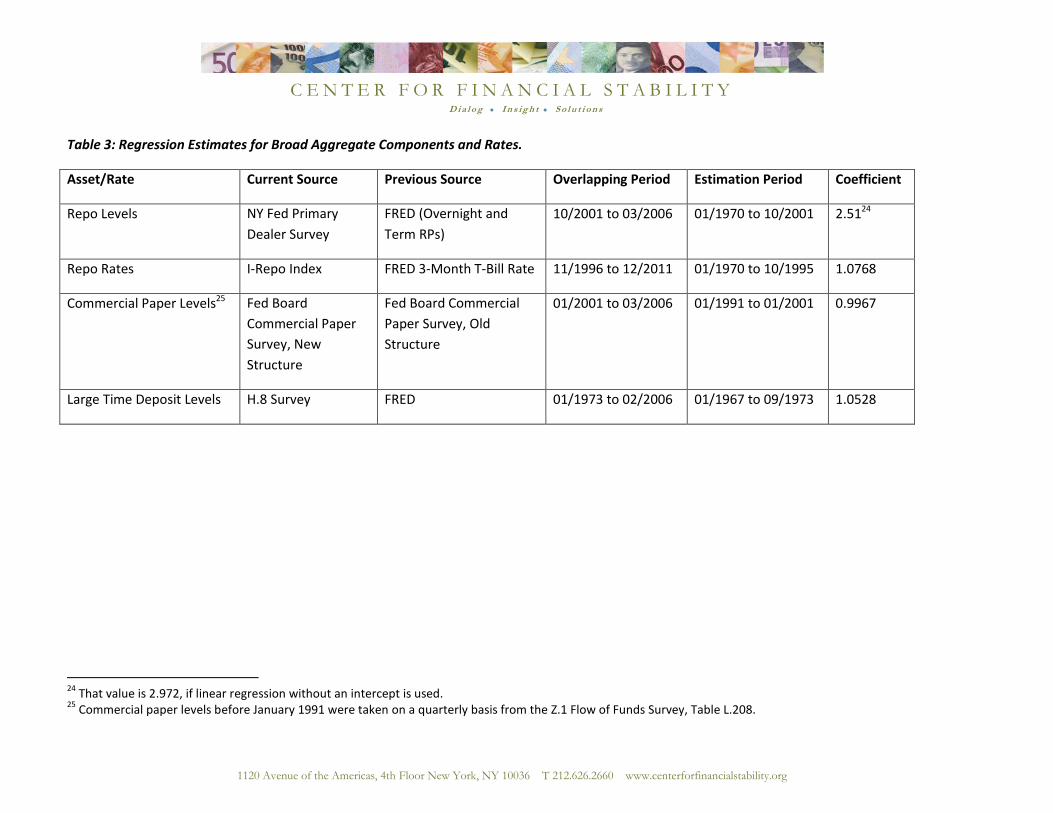
Table 3 is provided as a quick guide to these estimations. The table provides the sources, the

overlapping time period used in the regressions, the time periods within which estimations were used,

and the estimated values of the coefficients used to derive the past values.

23

A full description of the differences between the “old” and “new” structure surveys can be found at this website: http://www.federalreserve.gov/releases/cp/about.htm.



Table 3: Regression Estimates for Broad Aggregate Components and Rates.

Asset/Rate Current Source Previous Source Overlapping Period Estimation Period Coefficient

Repo Levels NY Fed Primary

Dealer Survey

FRED (Overnight and

Term RPs)

10/2001 to 03/2006 01/1970 to 10/2001 2.5124

Repo Rates I-Repo Index FRED 3-Month T-Bill Rate 11/1996 to 12/2011 01/1970 to 10/1995 1.0768

Commercial Paper Levels25 Fed Board

Commercial Paper

Survey, New

Structure

Fed Board Commercial

Paper Survey, Old

Structure

01/2001 to 03/2006 01/1991 to 01/2001 0.9967

Large Time Deposit Levels H.8 Survey FRED 01/1973 to 02/2006 01/1967 to 09/1973 1.0528

24

That value is 2.972, if linear regression without an intercept is used. 25

Commercial paper levels before January 1991 were taken on a quarterly basis from the Z.1 Flow of Funds Survey, Table L.208.



References

Anderson, R. G., & Jones, B. E. (2011). A Comprehensive Revision of the US Monetary Services (Divisia)

Indexes. Federal Reserve Bank of St. Louis Review, 93(5), 235-59.

Anderson, R. G., & Rasche, R. H. (2001). Retail Sweeps Prorams and Bank Reserves 1994 - 1999. Federeal

Reserve Bank of St. Louis Review, 83(1), 51-72.

Anderson, R. G., Jones, B. E., & T.D., N. (1997). Building New Monetary Services Indexes: Concepts, Data,

and Methods. Federal Reserve Bank of St. Louis Review, 79.1, 53-82.

Anderson, R., & Buol, J. (2005, November/December). Revisions to User Costs for the Federal Reserve

Bank of St. Louis Monetary Services. Federal Reserve Bank of St. Louis Review, 87(6), 735-749.

Bankrate.com. (2012). Track Economic Index Trends and Graph Financial Industry Rates. Retrieved from

http://www.bankrate.com/funnel/graph/

Barnett, W. (1980). Economic Monetary Aggregates: An Application of Index Number and Aggregation

Theory. Journal of Econometrics, 14, 11-48. Reprinted in Barnett and Serletis (2000), Chapter 2,

pp. 11-48.

Barnett, W. (1982). The Optimal Level of Monetary Aggregation. Journal of Money, Credit, and Banking,

14, 687-710. Reprinted in Barnett and Serletis (2000), Chapter 7, pp. 125-149.

Barnett, W. (2012). Getting it Wrong: How Faulty Monetary Statistics Undermine the Fed, the Financial

System, and the Economy. Cambridge, MA: MIT Press.

Barnett, W., & Serletis, A. (2000). The Theory of Monetary Aggregation. Amsterdam: North-Holland.

Barnett, W., & Spindt, P. (1982, May). Divisia Monetary Aggregates: Compilation, Data, and Historical

Behavior. Board of Governors of the Federal Reserve System Staff Study, 116.

Belongia, M., & Ireland, P. (2012). Where Simple Sum and Divisia Monetary Aggregates Part: Illustrations

and Evidence for the United States. University of Mississippi, working paper.

Cynamon, B., Dutkowsky, D., & Jones, B. (2006, Fall). Redefining the Monetary Aggregates: A Clean

Sweep. Eastern Economic Journal, 32(4), 661-672.

Diewert, W. (1999). Index Number Approaches to Seasonal Adjustment. Macroeconomic Dynamics, 3,

48-68.

European Central bank. (2000). Seasonal Adjustment of Monetary Aggregates and HICP for the Euro

Area. Frankfurt, Germany: European Central Bank.

Federal Reserve Bank of New York. (2012). Primary Dealer Statistics XML Data. Retrieved from

http://www.newyorkfed.org/xml/gsds_finance.html


-2-

Federal Reserve Board. (2003, March 23). Federal Reserve Statistical Release: H.6-Monety Stock

Measures. Retrieved from Discontinuance of M3.:

www.federalreserve.gov/releases/h6/20060323

Federal Reserve Board of Governors. (n.d.). Statistics and Historical Data. Retrieved 2012, from

http://www.federalreserve.gov/releases/h8/current/default.htm

Hanke, S. (2011, October). Malfeasant Central Bankers, Again. Energy Tribune.

Hanke, S. (2011, December). The Whigs Versus the Schoolboys. Globe Asia, 20-22.

Jones, B., Dutkowsky, D., & Elger, T. (2005). Sweep programs and optimal monetary aggregation. Journal

of Banking & Finances, 29, 483-508.

Serletis, A., & Gogas, P. (2012). Divisia Monetary Aggregates for Moentary Policy and Business Cycle

Analysis. University of Calgary, working paper.

Thornton, D., & Yue, P. (1992, November/December). An Extended Series of Divisia Monetary

Aggregates. Federal Reserve Bank of St. Louis Review, 74(6), 35-52.

Thorp, J. (2003). Change of seasonal adjustment method to X-12 ARIMA. Monetary and Financial

Statistics, 4-8.

TreasuryDirect. (2012). Monthly Statement of the Public Debt (MSPD) and Downloadable Files. Retrieved

2012, from http://www.treasurydirect.gov/govt/reports/pd/mspd/mspd.htm

United States Census Bureau. (2012, April). X-12 Arima. Retrieved April 2012, from US Census Bureau:

http://www.census.gov/srd/www/x12a/

The Center for Financial Stability (CFS) is a private, nonprofit institution focusing on global finance and

markets. Its research is nonpartisan. This publication reflects the judgments and recommendations of the

author(s). They do not necessarily represent the views of Members of the Advisory Board or Trustees,

whose involvement in no way should be interpreted as an endorsement of the report by either

themselves or the organizations with which they are affiliated.

Documents

The new CFS Divisia monetary aggregates: design