The Neighbor JoiningTree-Reconstruction Technique

Lecture 13

©Shlomo Moran & Ilan Gronau

2

Recall: Distance-Based Reconstruction:

• Input: distances between all taxon-pairs

• Output: a tree (edge-weighted) best-describing the

distances

0

30

980

1514180

171620220

1615192190

D

4 5

7 21

210 61

3

Requirements from Distance-Based Tree-Reconstruction Algorithms

1. Consistency: If the input metric is a tree metric, the returned tree should be the (unique) tree which fits this metric.

2. Efficiency: poly-time, preferably no more than O(n3), where n is the number of leaves (ie, the distance matrix is nXn).

3. Robustness: if the input matrix is “close” to tree metric, the algorithm should return the corresponding tree.

Definition: Tree metric or additive distances are distances which can be realized by a weighted tree.

A natural family of algorithms which satisfy 1 and 2 is called “Neighbor Joining”, presented next. Then we present one such algorithm which is known to be robust in practice.

4

The Neighbor Joining Tree-Reconstruction Scheme

1. Use D to select pair of neighboring leaves (cherries) i,j

2. Define a new vertex v as the parent of the cherries i,j

3. Compute a reduced (n-1)✕(n-1) distance matrix D’, over S’=S \ {i,j}{v}:

Important: need to compute distances from v to other vertices in S’, s.t.

D’ is a distance matrix of the reduced tree T’, obtained by

prunning i,j from T.

Start with an n✕n distance matrix D over a set S of n taxa (or vertices, or leaves)0 . .

0 . .

0 . .

0 .

0 .

0

0

D’

0 .. ..

0

0 ..

0 ..

0 ..

0

0

0

Di

v

j

5

The Neighbor Joining Tree-Reconstruction Scheme

4. Apply the method recursively on the reduced matrix D’, to get

the reduced tree T’.

5. In T’, add i,j as children of v (and possibly update edge

lengths).

Recursion base: when there are only two objects, return a tree with 2 leaves.

v

ji

0 . .

0 . .

0 . .

0 .

0 .

0

0

D’

v

T’

6

Consistency of Neighbor Joining

Theorem: Assume that the following holds for each input tree-metric D defined by some weighted tree T:

1.Correct Neighbor Selection: The vertices chosen at step 1 are cherries in T.

2.Correct Updating: The reduced matrix D’ is a distance matrix of some weighted tree T’ , which is obtained by replacing in T the cherries i,j by their parent v (T’ is the reduced tree).

Then the neighbor joining scheme is consistent: For each D which defines a tree metric it returns the corresponding tree T.

7

Consistency proofBy the correct neighbor selection and the correct updating assumptions, the algorithm:1. Selects i and j which are cherries in T.2.Computes a distance matrix D’ for the reduced subtree T’.

i jv k

By induction (on the number of taxa), the reduced tree T’ is correctly reconstructed.Hence T is correctly reconstructed by adding i,j as children of v

Consistent Neighbor Joining for Ultrametric Trees

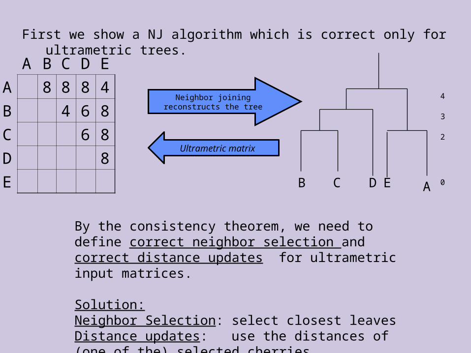
9

B C D AE

A B C D E

A 8 8 8 4

B 4 6 8

C 6 8

D 8

E

Neighbor joining reconstructs the tree

First we show a NJ algorithm which is correct only for ultrametric trees.

Ultrametric matrix

0

2

3

4

By the consistency theorem, we need to define correct neighbor selection and correct distance updates for ultrametric input matrices.

Solution:Neighbor Selection: select closest leavesDistance updates: use the distances of (one of the) selected cherries

10D Av

H

I

E

G

A i j D E

A 0 8 8 8 4

i 8 0 4 6 8

j 8 4 0 6 8

D 8 6 6 0 8

E 4 8 8 8 0

Neighbor selection:Two closest leaves

A Consistent Neighbor Joining Algorithm for Ultrametric Matrices:

A v D E

A 0 8 8 4

v 8 0 6 8

D 8 6 0 8

E 4 8 8 0

i j

v

Recursive constru

ction

Updating distances:For each k,

d’(v,k) = d(i,k)=d(j,k)

0

2

3

4

11

Robustness Requirement

In practice, it is important that the reconstruction algorithm will be robust: if the input matrix is not ultrametric, the algorithm should return a “close” ultrametric tree.

Such a robust neighbor joining technique for ultrametric trees is UPGMA. It achieves its robustness by the way it updates the distances in the reduced matrix.

UPGMA is used in many other applications, such as data mining.

12

UPGMA Clustering Unweighted Pair Group Method using Averages

UPGMA follows the “ultrametric neighbor joining scheme”. The only difference is in the distance updating procedure:

Each vertex i is identified with a cluster Ci , consisting of its descendants leaves.

Initially for each leaf i, there is a cluster Ci ={i}.

Neighbor joining: two closest vertices i and j are selected as neighbors, and replaced by a new vertex v. Set Cv = Ci Cj .

Updating distances: For each k , the distance from k to v is the average of the distances from the objects in Ck to the objects in Cv .

13

One iteration of UPGMAi and j are closest neighbors

•Replace i and j by v, •Update the distances from v to all other leaves:

i jv||||

||

ji

i

CC

C

D(v,k) = αD(i,k) + (1-α)D(j,k)

HW5 question: Show that this reduction formula guarantees the

UPGMA invariant: the distance between any two vertices i, j is the average of distances between the taxa in the corresponding clusters:

1( , ) ( , )

| || |i jp C q Ci j

d i j d p qC C

k

14

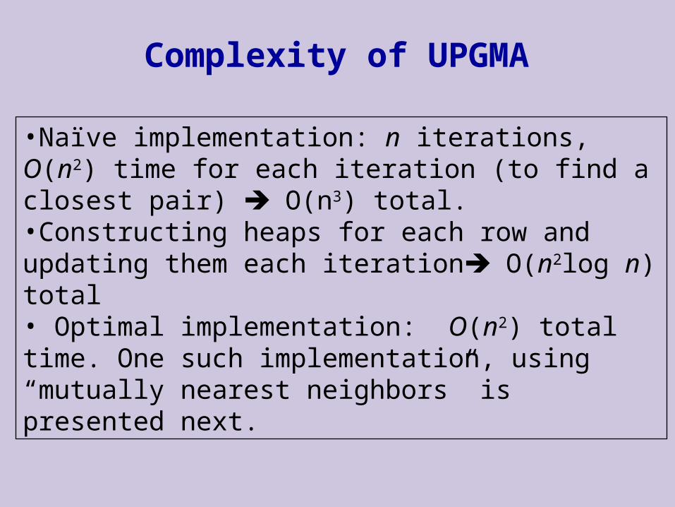
Complexity of UPGMA

•Naïve implementation: n iterations, O(n2) time for each iteration (to find a closest pair) O(n3) total.•Constructing heaps for each row and updating them each iteration O(n2log n) total• Optimal implementation: O(n2) total time. One such implementation, using “mutually nearest neighbors” is presented next.

15

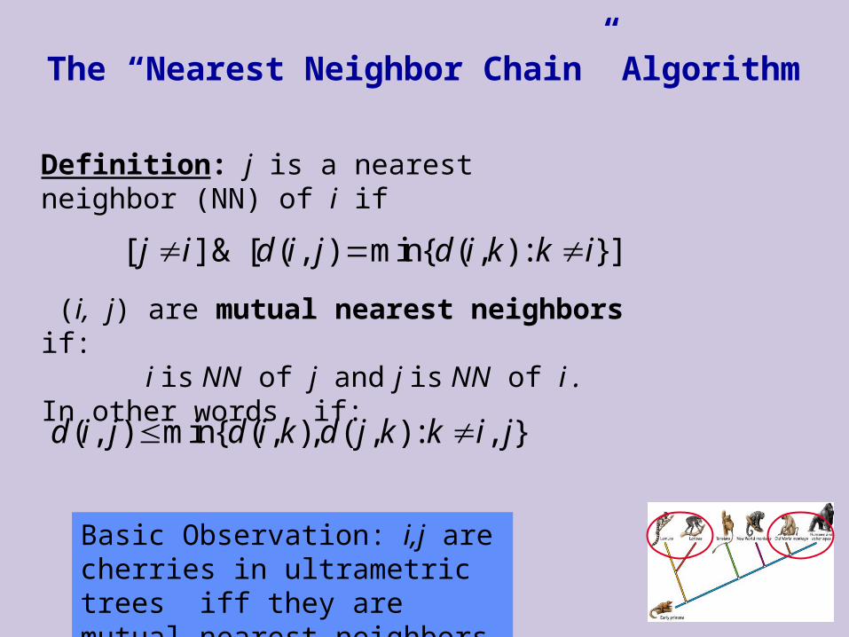
The “Nearest Neighbor Chain” Algorithm

Definition: j is a nearest neighbor (NN) of i if

[ ] & [ ( , ) min{ ( , ) : }]j i d i j d i k k i

( , ) min{ ( , ), ( , ) : , }d i j d i k d j k k i j

(i, j) are mutual nearest neighbors if: i is NN of j and j is NN of i .

In other words, if:

Basic Observation: i,j are cherries in ultrametric trees iff they are mutual nearest neighbors

16

Implementing UPGMA by

Mutual Nearest Neighbors

While(#vertices> 1) do:

• Choose i,j which are mutual nearest neighbors

• Replace i,j by a new vertex v , set Cv = C i Cj

• Reduce the distance matrice D to D’:For k≠v, D’(v,k) = αD(i,k) + (1-α)D(j,k)

|

| |

| | |i

i j

C

C C

17

00

0

00

00

00

0

0

Mutual NN

i0

i1

i0 i1

i1

i2

i2

Constructing Complete NN chain:

• ir+1 is a Nearest Neighbour of ir

• Final pair (il-1 ,il ) are mutual nearest neighbors.

D:

θ(n2) implementation the Mutual Nearest Neighbor:

Use nearest neighbors chain

3 6 4 5 8 2 6 9 3 2

5 7 3 2 4 8 1 9 7 6

2 1

C= (i0, i1,..,il ) is a Neraest Neighbor Chain if

D(ir ,ir+1) is minimal in row ir. i.e. ir+1 is a nearest

neighbour of ir.

C is a Complete NN chain if il-1 ,il are mutual

nearest neighbours.

18

An θ(n2) implementation using Nearest Neighbors Chains:

- Extend a chain until it is complete.

- Select final pair (i,j) for joining. Remove i,j from chain, join them to a new vertex

v, and compute the distances from v to all other vertices.

Note: in the reduced matrix, the remaining chain is still NN chain, i.e. ir+1 is still

the nearest neighbor of ir - since v didn’t become a nearest neighbor of any

vertex in the NN chain (since i and j were not)

Mutual NN

i j

19

Complexity Analysis:

• Count number of “row-minimum” calculations (each taking O(n) time) :- n-1 terminations throughout the execution- 2(n-1) Edge deletions 2(n-1) extensions - Total for NN chains operations: O(n2).- Updates: O(n) each iteration, total O(n2).- Altogether O(n2).

Consistent Neighbor Joining for General Tree Metrics

21

Neighbor Selection in General Weighted Trees

Unlike in ultrametric trees, closest vertices aren’t necessarily cherries in general weighed trees. Hence we need a different way to select cherries.

AB

CD

Idea: instead of using distances, use “LCA depths”

5

11

6

1

A B C D

A 0 3 6 8

B 0 7 7

C 0 12

D 0

22

LCA Depth

Let i,j be leaves in T, and let r i,j be a vertex in T.LCAr(i,j) is the Least Common Ancestor of i and j when r is

viewed as a root.If r is fixed we just write LCA(i,j) . dT(r,LCA(i,j)) is the “depth of LCAr(i,j)”.

ij

r

dT(r,LCA(i,j))

23

Matrix of LCA Depths

A weighted tree T with a designated root r defines a matrix of LCA depths:

A B C D E

A 8 0 0 3 5

B 9 5 0 0

C 8 0 0

D 7 3

E 7A

ED

CB

3423

2

5

4

3

dT(r,LCA(A,D)), = 3

r

24

Let T be a weighted tree, with a root r. For leaves i,j ≠r , let L (i,j)=dT(r,LCA(i,j))

Then i,j are cherries with parent v, iff:

Finding Cherries via LCA Depths

i j

r

, : ( , ) ( , ), ( , )k i j L i j L i k L j k

j

ij

v

In other words, i and j are cherries iff they have the same deepest ancestor. In this case we say that i and j are mutual deepest neighbors. Matrices of LCA depth are called LCA matrices. Next we charcterize such matrices.

25

LCA Matrices

Definition: A symmetric nonnegative matrix L is an LCA matrix iff

1. For all i, L(i,i)=maxjL(i,j).

2. It satisfies the “3 points condition”: Any subset of 3 indices can be labeled i, j, k s.t. L(i,j)= L(i,k)≤L(j,k) (i.e., the minimal value appears twice)

j i k

j 8 0 0 3 5

9 5 0 0

8 0 0

i 7 3

k 7

26

LCA Matrices Weighted Rooted Trees

Theorem: The following conditions are equivalent for a symmetric matrix L over a set S:

1. L is an LCA matrix.

2. There is a weighted tree T with a root r and leaves-set S, s.t. for each i,j in S:

L(i,j) = dT(r,LCA(i,j))

27

r

1

L:

L(A,A) = 7 =dT(r, A)

L(A,B) = 4 =dT(r,LCA(A,B))

זנים A B C D

A 7 4 3 1

B 9 3 1

C 6 1

D 7

Weighted Tree T rooted at r LCA Matrix:

28

LCA Matrices weighted tree T rooted at r

Proof of this direction is identical to the proof that an ultrametric matrix corresponds to distances in an ultrametric tree (that we saw last week, also in HW5).

Alternative proof is by an algorithm that constructs a tree from LCA matrix.

29

Input: an LCA matrix L over a set S.Output: A tree T with leaves in S {∪ r}, such that

• Stopping condition: If S={i} and L=[w] return the tree:

• Neighbor Selection: Choose mutual deepest neighbors i,j ,

• Reduction:

In the matrix L, delete rows i,j and add new row v, with values:L(v,v) L(i,j);For k≠v, L(v,k) L(i,k) //Note: L(i,k)=L(j,k)//Recursively call DLCA on the reduced matrix

• Neighbor connection:In the returned tree, connect i and j to v, with edge weights:

w(v,i) L(i,i)-L(i,j)w(v,j) L(j,j)-L(i,j)

DLCA: Neighbor Joining algorithm for LCA matrices:

, : ( , ) ( , ( , ))Ti j S L i j d r LCA i j

i

rw

30

One Iteration of DLCA:

A B C D E

A 8 0 0 3 5

B 0 9 5 0 0

C 0 5 8 0 0

D 3 0 0 7 3

E 5 0 0 3 7

V B C D E

V 5 0 0 3 5

B 0 9 5 0 0

C 0 5 8 0 0

D 3 0 0 7 3

E 5 0 0 3 7

Neighbor Connection (at the end)

v

EA

3 2

Replace rows A,E by V.

31

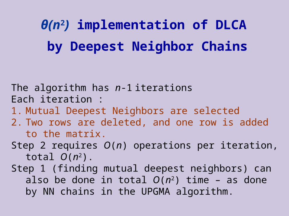
The algorithm has n-1 iterationsEach iteration :1. Mutual Deepest Neighbors are selected2. Two rows are deleted, and one row is added to the matrix.Step 2 requires O(n) operations per iteration, total O(n2).Step 1 (finding mutual deepest neighbors) can also be done in total

O(n2) time – as done by NN chains in the UPGMA algorithm.

θ(n2) implementation of DLCA

by Deepest Neighbor Chains

32

Running DLCA from (Additive) Distance Matrix D:

When the input is an (additive) distance matrix D, we apply on D the

following LCA reduction to obtain an (LCA) matrix L:

• Choose any leaf as a root r

• Set for all i,j : L(i,j) = ½(D(r,i) + D(r,j) - D(i,j))

• Run DLCA on L.Important observation: If D is an additive distance matrix corresponding to a

tree T, then L is an LCA matrix in which L(i,j)=dT(r,LCA(i,j))

i

j

r

33

A B C D r

A - 8 7 12 7

B - 9 14 9

C - 11 6

D - 7

r -

r

1

Example

A tree with the corresponding additive distance matrix

34

Use D to compute an LCA matrix L

D: L:זנים A B C D

A 7 4 3 1

B 9 3 1

C 6 1

D 7

זנים A B C D r

A - 8 7 12 7

B - 9 14 9

C - 11 6

D - 7

r -

1( , ) ( ( , ) ( , ) ( , ))

2L i j D r i D r j D i j

1( , ) (7 9 8) 4

2L A B

35

r

1

L:

L(A,A) = 7 =dT(r, A)

L(A,B) = 4 =dT(r,LCA(A,B))

זנים A B C D

A 7 4 3 1

B 9 3 1

C 6 1

D 7

The relation of L to the original tree:

36

Discussion of DLCA

• Consistency: If the input matrix L is an LCA matrix, then the output is guaranteed to be the unique weighted tree which realizes the LCA distances in L.

• Complexity: It can be implemented in optimal O(n2) time.• Robustness to noise:

• Theoretical: it has optimal robustness when 0≤ α ≤1.• Practical: it is inferior to other NJ algorithms – possibly due to the fact

that its neighbor-selection criterion is biased by the selected root r.

Next we present a neighbor selection criterion which use the original distance matrix. This criterion is known to be most robust to noise in practice.

37

Saitou & Nei’s Neighbor Joining Algorithm (1987)

select , which maximize the sum

( , ) ( , ) ( , ) ( 2) ( , )r r

i j

Q i j D r i D r j n D i j

~13,000 citations (Science Citation Index)

Implemented in numerous phylogenetic packages

Fastest implementation - θ(n3)

Usually referred to as “the NJ algorithm”

Identified by its neigbor selection criterion

Saitou & Nei’s neighbor-

selection criterion

38

Consistency of Seitou&Nei method

Theorem (Saitou&Nei) Assume all edge weights of T are positive. If Q(i,j)=max{i’,j’} Q(i’,j’) , then i and j are cherries in the tree.

Proof: in the following slides.

( , ) ( , ) ( , ) ( 2) ( , )r r

Q i j D r i D r j n D i j

,

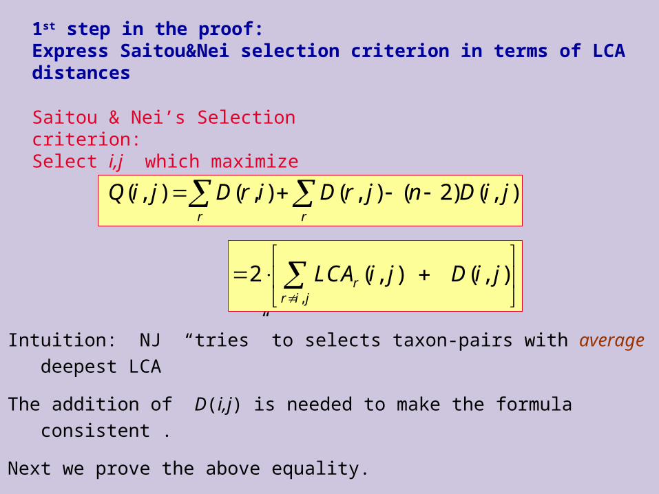
2 ( , ) ( , )rr i j

LCA i j D i j

Intuition: NJ “tries” to selects taxon-pairs with average deepest LCA

The addition of D(i,j) is needed to make the formula consistent .

Next we prove the above equality.

Saitou & Nei’s Selection criterion:Select i,j which maximize

( , ) ( , ) ( , ) ( 2) ( , )r r

Q i j D r i D r j n D i j

1st step in the proof: Express Saitou&Nei selection criterion in terms of LCA distances

40

Proof of equality in previous slide

, ,

,

( , ) ( , ) ( , ) ( , ) ( , ) ( 2) ( , )

[ ( , ) ( , ) ( , )] 2 ( , )

r i j r i j

r i j

Q i j D i j D i r D j i D j r n D i j

D i r D j r D i j D i j

-2d(r,LCAr(i,j))

,

2 ( , ) ( , ( , ))rr i j

D i j d r LCA i j

ri rj

41

2nd step in proof:Consistency of Saitou&Nei Neighbor Selection

,

We need to show that a pair of leaves , which maximize

'( , ) ( , ) / 2 ( , ) ( , ( , ))

must be cherries. First we express ' as a sum of edge weights.

ur i j

i j

Q i j Q i j D i j D r LCA i j

Q

, ( , ) ( , )

'( , ) ( , ) ( , ( , )) ( ) ( ) ( )r ir i j e path i j e path i j

Q i j D i j D r LCA i j w e N e w e

For a vertex i, and an edge e:Ni(e) = |{rS : e is on path(i,r)}|Then:

Note: If e’ is a “leaf edge”, then w(e’) is added exactly once to Q(i,j).

ij

rRest of T

e

path(i,j)

42

Let (see the figure below):• path(i,j) = (i,...,k,j).• T1 = the subtree rooted at k. WLOG that T1 has at most n/2 leaves. •T2 = T \ T1.

ij

k

T1

T2

Assume for contradiction that Q’(i,j) is maximized for i,j which are not cherries.

i’j’Let i’,j’ be any two cherries in T1. We

will show that Q’(i’,j’) > Q’(i,j).

Consistency of Saitou&Nei (cont)

43

ij

k

T1

T2

Proof that Q’(i’,j’)>Q’(i,j):

i’j’

( , ) ( , )

'( ', ') ( ', ')

'( , ) ( ) ( ) ( )

'( ', ') ( ) ( ) ( )

ie p i j e p i j

ie p i j e p i j

Q i j w e N e w e

Q i j w e N e w e

Each leaf edge e adds w(e) both to Q’(i,j) and to Q’(i’,j’), so we can ignore the contribution of leaf edges to both Q’(i,j) and Q’(i’,j’)

Consistency of Saitou&Nei (cont)

44

ij

k

T1

T2i’

j’

Location of internal edge e

# w(e) added to Q’(i,j)

# w(e) added to Q’(i’,j’)

epath(i,j) 1 Ni’(e)≥2

epath(i’,j) Ni (e) < n/2 Ni’(e) ≥ n/2

eT\path(i,i’) Ni (e) = Ni’(e)

Since there is at least one internal edge e in path(i,j), Q’(i’,j’) > Q’(i,j). QED

Contribution of internal edges to Q(i,j) and to Q(i’,j’)

Consistency of Saitou&Nei (end)

45

Initialization: θ(n2) to compute Q(i,j) for all i,jL.

Each Iteration: O(n2) to find the maximal Q(i,j), and to update the

values of Q(x,y)

Total: O(n3)

Complexity of Seitou&Nei NJ Algorithm

A characterization of additive metrics:The 4 points condition

Ultrametric distances and LCA distances were shown to satisfy “3 points conditions”.

Tree metrics (aka “additive distances”) have a characterization known as the “4 points condition”, which we present next.

47

Distances on 3 objects are always realizable by a (unique) tree with one internal node.

( , )( , )( , )

d i j a bd i k a cd j k b c

ab

c

i

j

k

m

For instance0

2

1 )],(),(),([),( jidkjdkidmkdc

i j k

i 0 a+b a+c

j 0 b+c

k 0

48

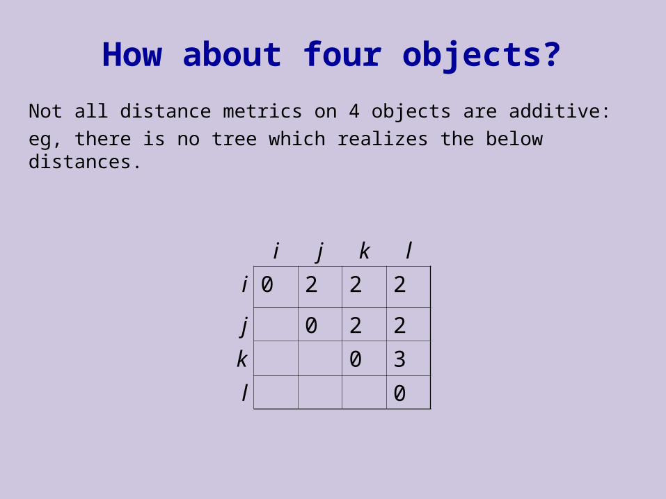
How about four objects?

Not all distance metrics on 4 objects are additive:

eg, there is no tree which realizes the below distances.

i j k l

i 0 2 2 2

j 0 2 2

k 0 3

l 0

49

The Four Points Condition

A necessary condition for distances on four objects to be additive: its objects can be labeled i,j,k,l so that:

d(i,k) + d(j,l) = d(i,l) +d(k,j) ≥ d(i,j) + d(k,l)

Proof: By the figure...

{{i,j},{k,l}} is a “split” of {i,j,k,l}.

ik

lj

50

The Four Points Condition

Definition: A distance metric satisfies the four points condition iff any subset of four objects can be labeled i,j,k,l so that:

d(i,k) + d(j,l) = d(i,l) +d(k,j) ≥ d(i,j) + d(k,l)

ik

lj

51

Equivalence of the Four Points Condition and the Three Points Condition

rk

lj

4 ( , ) ( , ) ( , ) ( , ) ( , ) ( , )

( , ) ( , ) ( , ) ( , ) and ( , ) ( , ) ( , ) ( , )

2 ) ( , ) ( , ) ( , ) ( , ) ( , ) ( , )[ 2 )( , ( , ) ( , ( ]

( , ) ( , ,

)

)

,

( )

PC d r k d j l d r l d j k d r j d k l

d r k d j k d r l d j l d r l d k l d r j d j k

d rd r LCA k l d r LCA j kk d r l d k l d r k d r j d j k

d r j d r l d j l

( , ( , )2 ) 3d r LCA l PCj

i.e., a matrix D satisfies the 4PC on all quartets that include r iff the LCA reduction applied on D and r outputs a matrix L which satisfies the 3PC for LCA distances.

52

The Four Points ConditionTheorem: The following 3 conditions are equivalent for a distance matrix D on a

set S of L objects

1. D is additive

2. D satisfies the four points condition for all quartets in S.

3. There is a vertex r in S, s.t. D satisfies the 4 points condition for all quartets that include r.

ik

lj

53

The Four Points Condition

Proof: we’ll show that 1231.1 2Additivity 4P Condition satisfied by all quartets: By the figure...

ik

lj

23: trivial

54

Proof that 3 1

The proof is as follows:• All quartets in D which include r satisfy the 4PC • The matrix L obtained by applying the LCA reduction on D

and r is an LCA matrix• The tree T output by running DLCA on L realizes the LCA

depths in L• T realizes the distances in D.

4PC on all quartets which include r additivity