Embed Size (px)
Citation preview
THE NAVIER-STOKES-VOIGHT MODEL FOR IMAGE INPAINTING
M.A. EBRAHIMI, MICHAEL HOLST, AND EVELYN LUNASIN
ABSTRACT. In this paper we investigate the use of the 2D Navier-Stokes-Voight (NSV)model for use in algorithms and explore its limits in the context of image inpainting. Webegin by giving a brief review of the work of Bertalmio et. al. in 2001 on exploiting ananalogy between the image intensity function for the image inpainting problem and thestream function in 2D incompressible fluid. An approximate solution to the inpaintingproblem was then obtained by numerically approximating the steady state solution of the2D Navier-Stokes vorticity transport equation, and simultaneously solving the Poissonproblem between the vorticity and stream function, in the region to be inpainted. Thiselegant approach allows one to produce an approximate solution to the image inpaint-ing problem by using techniques from computational fluid dynamics (CFD). Recently,the three-dimensional (3D) Navier-Stokes-Voight (NSV) model of viscoelastic fluid, wassuggested by Cao, et. al. as an inviscid regularization to the 3D Navier-Stokes equations.We give some background on the NSV mathematical model, describe why it is a goodcandidate sub-grid-scale turbulence model, and propose this model as an alternative forimage inpainting. We describe an implementation of inpainting use the NSV model, andpresent numerical results comparing the resulting images when using the NSE and NSVfor inpainting. Our results show that the NSV model allows for a larger time step toconverge to the steady state solution, yielding a more efficient numerical process whenautomating the inpainting process. We compare quality of the resulting images usingsubjective measure (human evaluation) and objected measure (by calculating the peaksignal-to-noise ratio (PSNR), also known as peak signal-to-reconstructed measure). Wealso present some new theoretical results based on energy methods comparing the suf-ficient conditions for stability of the discretization scheme for the two model equations.These theoretical and numerical studies shed some light on what can be expected fromthis category of approach when automating the inpainting problem.
CONTENTS
1. Introduction 22. Image Inpainting Using Fluid Models 32.1. Inpainting Using the Navier-Stokes Equations 42.2. Alpha Models and the Navier-Stokes-Voight (NSV) Equations 52.3. The Alpha Model as Sub-Grid-Scale Turbulence Model 72.4. Navier-Stokes-Voight for Image Inpainting 73. Numerical Comparison NSE and NSV for Image Inpainting 83.1. Stability Behavior of NSE and NSV for Inpainting 83.2. Comparing the Efficiency of NSE and NSV for Inpainting 104. Some Supporting Theoretical Results 124.1. Uniqueness of Steady State Solutions for Boundary Driven Flows 144.2. Stability Analysis of the Scheme based on 2D NSE 154.3. Stability Analysis of the Scheme based on 2D NSV 194.4. Stability Analysis of a Semi-Implicit Scheme based on 2D NSE 215. Summary 236. Acknowledgments 24References 24
Date: December 15, 2009.Key words and phrases. Navier-Stokes-Voight, sub-grid scale turbulence model, fluid mechanics,
image inpainting.MH was supported in part by NSF Awards 0715146 and 0915220.
ME and EL were supported in part by NSF Award 0715146.1
arX
iv:0
901.
4548
v3 [
mat
h.N
A]
15
Dec
200
9
2 M.A. EBRAHIMI, M. HOLST, AND E. LUNASIN
1. INTRODUCTION
Image inpainting (inpainting for short) is the process of correcting a damaged im-age by filling in the missing or altered data of an image with a better suited data forthat region. The idea is to fill in the damaged part of an image using the informationfrom surrounding areas. The goal of researchers in this area is to develop algorithms forautomatic digital inpainting which mimics the basic manual techniques used by a profes-sional restorer. In 2001, Bertalmio, et. al. built a method based on an analogy betweenimage intensity and the stream function in a two-dimensional (2D) incompressible fluid.The solution to the inpainting problem is then obtained by numerically approximatingthe steady state solution of the 2D Navier-Stokes vorticity transport equation, for somesmall viscosity, and simultaneously solving the Poisson problem between the vorticityand stream function in the region to be inpainted. This approach enables automation ofthe inpainting process by which inpainting is done using techniques from computationalfluid dynamics (CFD). However, difficulties which arise in CFD are also inherited.
For inpainting, the viscosity in the fluid model should be as small as possible to pre-serve edges. However, CFD simulation of high Reynolds number flows (flows with verysmall viscosity) requires very fine mesh in order to resolve the wide range of scales ofmotion contributing to the dynamics of the flow. Sub-grid scale modeling is an alternativethat reduces the computational requirements when simulating turbulent flows. Recently,the three-dimensional (3D) Navier-Stokes-Voight (NSV) model of viscoelastic fluid,
−α2∆ut + ut − ν∆u+ (u · ∇)u+∇p = f,
∇ · u = 0,(1.1)
with initial condition u(x, 0) = uin(x) was suggested by Cao, et. al. as an inviscidregularization to the 3D Navier-Stokes equations (NSE), where the length-scale α isconsidered as the regularizing parameter, u is the velocity of the fluid with viscosityν > 0, p is the pressure and f is the body force. Note that when α = 0, we re-cover the Navier-Stokes equations of motion. The system (1.1) was first introduced in1973 by Oskolkov (see [30, 31]) as a model of a motion of linear, viscoelastic fluid.In that setting, α is thought of as a length-scale parameter characterizing the elasticityof the fluid. The 3D NSV model is shown to be globally well-posed [30, 31] and hasa finite-dimensional global attractor [21], making it an attractive sub-grid scale turbu-lence model for numerical simulation. In the presence of physical boundaries, the aboveregularization of the NSE is different in nature from other alpha regularization modelsin [7, 8, 9, 10, 11, 13, 20, 24, 29] (see also Section 2.2), because it does not requireadditional boundary conditions.
In this paper, we investigate a new approach which arises by combining the recenttechnique in [4], which uses ideas from classical fluid dynamics to propagate isophotelines, and recent results in [8, 22, 21], which studies the NSV model of viscoelastic fluidas a candidate sub-grid scale turbulence model for purposes of numerical simulation.Other PDEs have been proposed recently for example in [6, 34] which are possibly con-sidered to be more efficient and perhaps easier to implement. Of particular interest tous in this area is to explore different sub-grid scale turbulent models applied to imageinpainting. For the reasons outlined above, we have chosen this particular turbulencemodel to study in the context of inpainting. Using this new model, we will study theeffect of the regularization parameter α (which one can think of as the filter width) onquality and efficiency of inpainting automation. As part of our investigation of 2D NSVfor inpainting, we examine the differences between the 2D NSV model and the 2D NSE
THE NAVIER-STOKES-VOIGHT MODEL FOR IMAGE INPAINTING 3
for inpainting. We look at semi-implicit forward-time upwind method for both NSV andNSE and compare their stability and efficiency. We will refer to these numerical meth-ods by their corresponding mathematical model: NSV and NSE numerical model. Ournumerical results show the NSV model, in comparison to NSE, yields a more stable solu-tion to the inpainting process. That is, the NSV can be computed with larger time-steps,reducing the computational expense in the automated inpainting procedure. However,we also study the efficiency of the calculation of the model equations as well as the qual-ity of the resulting images. We hope that these theoretical and numerical studies shedsome light on what can be expected from this category of approach when automating theinpainting problem.
This paper is organized as follows. In Section 2 we review the work of Bertalmio et.al. in [4] on exploiting an analogy between image intensity and the stream function in 2Dincompressible fluid. In Section 2.2 we give some background on the NSV mathematicalmodel, discuss why it is a good candidate sub-grid-scale turbulence model, and argue thatit makes for a plausible alternative model for inpainting. In Section 3 we describe ourimplementation, and then present our numerical results, comparing the resulting imageswhen using the NSE and NSV for inpainting. The results show the NSV model allows forlarger time steps to converge to the steady state solution yielding a more efficient numeri-cal process when automating the inpainting process. We compare quality of the resultingimages using subjective measure (human evaluation) and objected measure (by calculat-ing the peak signal-to-noise ratio (PSNR), also known as peak signal-to-reconstructedmeasure). We also give approximate operation counts needed by the two models to con-verge to steady state solution for some fixed tolerance. In Section 4 we present somesupporting theoretical results. In Section 4.1, we summarize some existing results on thedependence of uniqueness of the solution to the inpainting problem on the image at theboundary, viscosity and on the size of the inpainting region. In Sections 4.2, 4.3, and4.4, we establish some new results comparing the NSE and NSV in terms of stabilityconditions. We describe the discretization under consideration, and following [33], de-rive sufficient conditions for stability based on energy methods, establishing results thatsupport our numerical results. In Section 5 we summarize our results and outline somefuture directions for this work.
2. IMAGE INPAINTING USING FLUID MODELS
In this section we present a summary of the approach in [4] for automating the inpaint-ing process motivated by ideas from classical fluid dynamics. The idea is to propagateisophote lines from the exterior into the region to be inpainted, which we denote as Ω,using the 2D NSE for fluid dynamics. Throughout the paper, we denote the digital gray-scale image by I , an m × n matrix with gray-scale value 0 to 255 at each pixel, and Dbe the set of points (x, y) where I is defined. The value 0 represents black and the value255 represents white. The values in between are different gray levels between black andwhite.
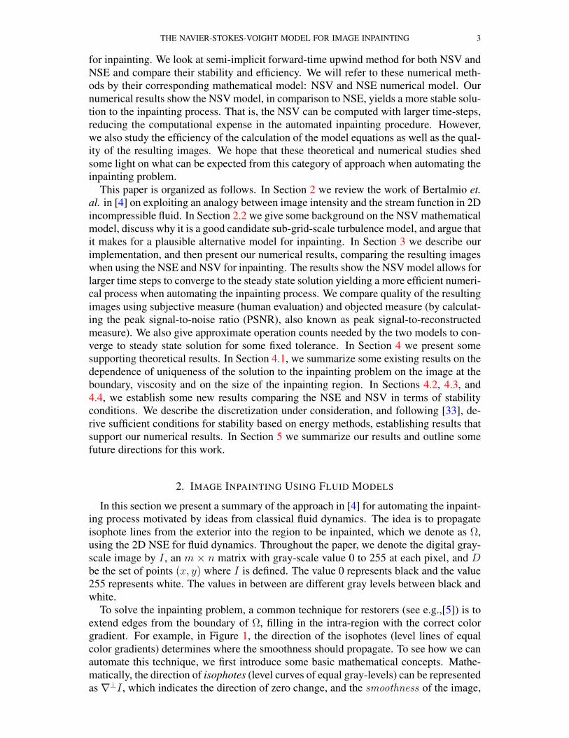
To solve the inpainting problem, a common technique for restorers (see e.g.,[5]) is toextend edges from the boundary of Ω, filling in the intra-region with the correct colorgradient. For example, in Figure 1, the direction of the isophotes (level lines of equalcolor gradients) determines where the smoothness should propagate. To see how we canautomate this technique, we first introduce some basic mathematical concepts. Mathe-matically, the direction of isophotes (level curves of equal gray-levels) can be representedas ∇⊥I , which indicates the direction of zero change, and the smoothness of the image,
4 M.A. EBRAHIMI, M. HOLST, AND E. LUNASIN
FIGURE 1. This image shows the direction of the isophotes and where thesmoothness should propagate.
can be represented by ∆I , where ∆ is the usual Laplacian operator (see [4] and refer-ences therein).
2.1. Inpainting Using the Navier-Stokes Equations. In [5], Bertalmio, et. al. pro-posed that the solution I∗ can be approximated with the steady solution to the PDE ofthe form
It = ∇⊥I · ∇∆I + ν∇ · (g(|∇I|)∇I), (2.1)for small ν > 0, where the anisotropic diffusion is added to preserve the edges. We willlist below a few diffusivity functions g that are used in the literature. To be more precise,the main goal is to find the solution I∗ such that the level curves of ∆I∗ almost parallelto ∇⊥I∗, that is,
∇⊥I∗ · ∇∆I∗ ' 0. (2.2)Bertalmio et. al. [4] exploited an analogy between the image of intensity function I andthe stream function in a 2D incompressible fluid. To see this, we recall the vorticity-stream formulation of the 2D NSE,
∂ω
∂t+ v · ∇ω = ν∆ω. (2.3)
Here v = ∇⊥Ψ is the velocity, where Ψ is the stream function and ω = ∇ × v is thevorticity. If the viscosity ν is zero, the steady state solution for the stream-function Ψ in2D satisfies
∇⊥Ψ · ∇∆Ψ = 0. (2.4)
The similarity between (2.2) and (2.4) allows one to develop methods for the inpaint-ing problem using techniques from fluid dynamics. For the image inpainting problem,instead of simulating (2.3), we compute the following numerically:
∂ω
∂t+ v · ∇ω = ν∇ · (g(|∇ω|)∇ω), (2.5)
where g accounts for the anisotropic diffusion (edge preserving diffusion) to sharpen theimage. At each time step, we solve the Poisson equation:
∆I = ω, I|∂Ω = I0, (2.6)
where the boundary values I0 are derived from the values of I in D − Ω.We recall that other PDEs have been proposed recently (cf. [6, 34]) which have been
shown to more efficient and perhaps easier to implement. Here, our main interest is toexplore different sub-grid scale turbulent models applied to image inpainting. The ideais to test different sub-grid scale turbulence models instead of simulating the NSE (or theequation in (2.5)) for purposes of finding the solution to the image inpainting problem
THE NAVIER-STOKES-VOIGHT MODEL FOR IMAGE INPAINTING 5
for reduced computational requirements. Modifying the function g appropriately in (2.5)can also add to the accuracy of preserving the edges and hence give a more accurateimage inpainting. In (2.5) we noted that for the image inpainting, the dissipation term inthe NSE was modified to accommodate anisotropic diffusion. If g = 1, we recover theusual NSE with isotropic diffusion. There has been extensive analysis of various types ofanisotropic filtering, see for example [35]. In our numerical simulation of equation (2.5)we have used several different diffusivity functions, namely,
g(s) =
[1 +
( sk2
)2]−1
, g(s) = exp(− s
k2
), g(s) =
[1 +
( sk2
)]−1
,
where k is a predefined diffusion parameter. For the particular test cases performed,we observed no significant difference in the numerical solution to the image inpaintingproblem.
x
y
Original image with noise
50 100 150 200 250
50
100
150
200
250
50
100
150
200
(a)
x
y
Recovered image with NSE: =2, dt = .0001
50 100 150 200 250
50
100
150
200
250
50
100
150
200
(b)
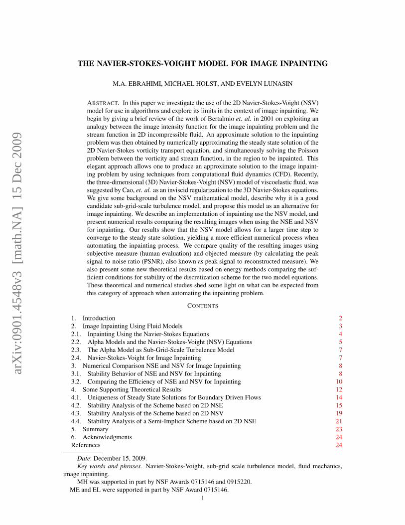
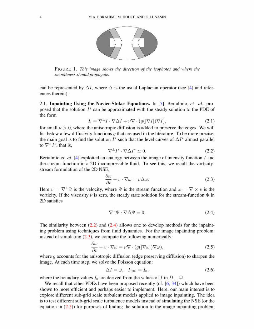
FIGURE 2. This is an example of image inpainting resulting from the steadystate solution of the Navier-Stokes equations (with anisotropic diffusion to pre-serve edges) with viscosity ν = 2. The time-step dt was set to .0001 to guaranteeconvergence of the numerical solution.
Just as an illustration of the idea, we give a simple numerical experiment. In Fig-ure 2.1a, we took the photo of Alexander Ebrahimi with a noise mask as a test case.We run the Navier-Stokes equations (NSE) with anisotropic diffusion until its steadystate [4], and recovered the picture in Figure 2.1b. The iterative inpainting process writ-ten in MATLAB took 24 iterations with a tolerance of 0.0001, in about 1.84 seconds ona laptop computer with a Intel(R) 1.60 GHz CPU. The grid for the inpainting region is49× 59 pixels.
2.2. Alpha Models and the Navier-Stokes-Voight (NSV) Equations. The NSV equa-tions (1.1) were suggested as a regularization model for the 3D NSE, where the length-scale α is considered as the regularizing parameter. The system (1.1) was first introducedin 1973 by Oskolkov (see [30, 31]) as a model of a motion of linear, viscoelastic fluid.In that setting, α is thought of as a length-scale parameter characterizing the elasticityof the fluid. As noted in [22, 21], the addition of the term −α2∆ut regularizes the 3DNSE which makes it globally well-posed [8, 30] and it changes the parabolic charac-ter of the original Navier-Stokes equations where in this case one does not observe animmediate smoothing of the solutions as usually expected in parabolic PDEs. Instead,the equations behave like a damped hyperbolic system. Despite the damped hyperbolic
6 M.A. EBRAHIMI, M. HOLST, AND E. LUNASIN
behavior, it was shown in [22] that the solutions to the 3D NSV equations lying on theglobal attractor posses a dissipation range. This property supports the claim that indeed,the NSV equations can be used as a sub-grid scale turbulence model. This type of invis-cid regularization (that is, a regularization technique without introducing extra viscousor hyperviscous terms) has been used for 2D surface quasi-geostrophic (SQG) model([23]), see also [3] for the Birkhoff-Rott equation, induced by the 2D Euler-α equationsfor vortex sheet dynamics and [25] for the 3D Magnetohydrodynamics (MHD) equations.
There is an interesting literature behind the rediscovery of the NSV equation as aturbulence model. It can be traced back from the early study of 3D Navier-Stokes-α(NS-α) turbulence model in 1998 (also known as the viscous Camassa-Holm equations(VCHE) and Lagrangian averaged Navier-Stokes-α (LANS-α) model, which can be writ-ten as [15, 16, 19, 28]
∂tv − ν∆v − u×∇× v = −∇p+ f,
∇ · u = ∇ · v = 0,
v = (I − α2∆)u,
(2.7)
with u(x, 0) = uin(x). The parameter α can be viewed as the length scale associatedwith filter width smoothing v to obtain u, with filter associated with the Green’s function(Bessel potential) of the Helmholtz operator (I − α2∆). The system is supplementedwith periodic boundary conditions in a box [0, L]3.
The inviscid and unforced version of the 3D NS-α was introduced in [19] based onthe Hamilton variational principle subject to the incompressibility constraint div v = 0.By adding the viscous term −ν∆v and the forcing f in an ad hoc fashion, the authorsin [9, 10, 11] and [16] obtain the NS-α system which they named, at the time, the vis-cous Camassa-Holm equations (VCHE), also known as the Lagrangian averaged Navier-Stokes-α model (LANS-α). In [9, 10, 11] it was found that steady state solutions of the3D NS-α model compared well with averaged experimental data from turbulent flowsin channels and pipes for large Reynolds numbers. This led researchers [9, 10, 11] tosuggest that the NS-α model be used as a closure model for the Reynolds averaged equa-tions. Since then, an entire family of ‘α’- models has been found which provide similarsuccessful comparison with empirical data – among these are the Clark-α model [7],the Leray-α model [13], the modified Leray-α model [20] and the simplified Bardinamodel [8, 24] (see also [29] for a family of similar models). We focus our attention onthe simplified Bardina model:
∂tv − ν∆v + (u · ∇)u = −∇p+ f,
∇ · u = ∇ · v = 0,
v = u− α2∆u,
(2.8)
with initial condition u(x, 0) = uin(x). The equation above was introduced and studiedin [24] supplemented with periodic boundary conditions. Notice that consistent with allthe other alpha models, the above system is the Navier-Stokes system of equations whenα = 0, i.e. u = v. In [8], the viscous and inviscid simplified Bardina models wereshown to be globally well-posed. It was also shown that the viscous simplified Bardinamodel has a finite dimensional global attractor. In [8] it was observed that the inviscidsimplified Bardina model, is equivalent to the following modification of the 3D Euler
THE NAVIER-STOKES-VOIGHT MODEL FOR IMAGE INPAINTING 7
equations
−α2∆∂u
∂t+∂u
∂t+ (u · ∇)u+∇p = f,
∇ · u = 0,(2.9)
with initial condition u(x, 0) = uin. In particular, it is equal to the Euler equations whenα = 0. Following this observation, Cao, et. al. [8] proposed the inviscid simplifiedBardina model as regularization of the 3D Euler equations that could be used for simu-lations of 3D inviscid flows. Inspired by the above model, Cao, et. al then proposed thefollowing regularization of the 3D Navier-Stokes equations
−α2∆∂u
∂t+∂u
∂t− ν∆u+ (u · ∇)u+∇p = f,
∇ · u = 0,(2.10)
with initial condition u(x, 0) = uin, and subject to either periodic boundary condition orthe no-slip Dirichlet boundary condition u|∂Ω = 0. In the presence of physical bound-aries the above regularization (2.10) of the Navier-Stokes equations, is different in naturefrom any of the other alpha regularization models, because it does not require any addi-tional boundary conditions.
This newest addition to the family of ‘α’ models was later on discovered to havealready existed in the literature known as the Navier-Stokes Voight equations but as amodel for viscoelastic fluids [30, 31]. As mentioned earlier, the α in that setting repre-sents the elasticity of the fluid.
2.3. The Alpha Model as Sub-Grid-Scale Turbulence Model. In addition to the re-markable match of explicit analytical steady state solutions of the alpha models to theexperimental data in channels and pipes, the validity of the first alpha model, namely theNS-αmodel, as a sub-grid scale turbulence model was also tested numerically in [12, 28].In the numerical simulation of the 3D NS-αmodel, the authors of [12, 17, 18, 28] showedthat the large scale (to be more specific, those scales of motion bigger than the lengthscale α) features of a turbulent flow is captured. For scales of motion smaller than thelength scale α, the energy spectra decays faster in comparison to that of NSE. This nu-merical observation has been justified analytically in [15]. In direct numerical simulation,the fast decay of the energy spectra for scales of motion smaller than the supplied filterlength represents reduced grid requirements in simulating a flow. The numerical studyof [12] gives the same results, which also hold for the Leray-α model in [13, 17].
In [26] it was observed that the scaling exponent of the energy spectrum of the 2DNavier-Stokes-α model (NS-α), for wave numbers k such that kα 1, is k−7. A pos-teriori, it was observed that this scaling corresponding to that predicted by assumingthat the dynamics for kα 1 was governed by the characteristic time scale for flux ofthe conserved enstrophy. This observation led researchers [26] to speculate that (in gen-eral) the unknown scaling exponent for any α-model may be predicted by the dynamicaltime scales for the dominant conserved quantity for that model in the regime kα 1.This speculation is verified to be correct in [27], where numerical simulations of the 2DLeray-α model were presented.
2.4. Navier-Stokes-Voight for Image Inpainting. The main difference between NSVand other alpha models is that it needs no additional boundary conditions in the presenceof physical boundaries. This makes NSV a natural alternative to NSE for inpainting.In order to solve the inpainting problem we need to compute the solution to (2.4). Weapproximate it with the steady state solutions of (2.5) with viscosity ν > 0. As noted
8 M.A. EBRAHIMI, M. HOLST, AND E. LUNASIN
in [4] the presence of viscosity is needed to have a unique steady-state solution and itsstability depends on how big or small is the viscosity. It is well-known that for very highReynolds number flows (ie very small viscosity ν), direct numerical simulation of theNSE, requires computational resources which cannot be accessed easily. For purposesof direct numerical simulations, the NSV equations were proposed as a sub-grid scaleturbulence model. Here we would like to investigate the effects of this regularized equa-tions to image inpainting. Notice that the steady state solution to the NSV equations in(1.1) matches the steady state solution to the NSE. We expect that by using the NSV,the convergence to the steady state solution will be at a much faster rate reducing thecomputational cost.
3. NUMERICAL COMPARISON NSE AND NSV FOR IMAGE INPAINTING
We simulate the inviscid 2D NSV with anisotropic diffusion (artificial viscosity)
− α2 ∂
∂t∆ω +
∂ω
∂t+ u · ∇ω = ν∇ · (g(|∇ω|)∇ω), (3.1)
where, ω = ∇ × u. Notice that when α = 0, we recover (2.5). Using a forward timeup-wind finite-difference scheme [2], we solve for ω(n+1)
i,j in the discretized equation:
(1− α2∆)ωn+1i,j − νdt (∂x(gω
n+1x ) + ∂y(gω
n+1y )) = (1− α2∆)ωni,j
+ dt
[−|un1 | sgn(un1 )
ωni+ sgn(un1 ),j − ωni,jdx
− |un2 | sgn(un2 )ωni,j+ sgn(un
2 ) − ωni,jdy
].
(3.2)
Our numerical experiments can be summarized into three categories: test for stability,test for efficiency and test for quality. In section 3.1, we present some test cases showingthat for a given time stepping size, the gray-level blows up when the inpainting is doneusing NSE while the inpainting using NSV produced a stable solution. We give theoret-ical arguments in the appendix which in some sense support these numerical results. Itis worthwhile to mention that using an explicit numerical scheme for both the 2D NSEand 2D NSV equations, one can see a nice advantage of using NSV instead of the NSEin automating the inpainting problem in terms of CFL condition when we for simplicityignore the nonlinear term in the governing equations. In particular, the usual stiffnessof the NSE by discretizing the linear part explicitly is no longer present for NSV. In theAppendix, we present rigorous argument for the stability condition when the nonlinearterm is taken into consideration. In section 3.2 we present some numerical studies usingNSE and NSV for different values of α. We look at the effect of the parameter α onthe quality of the resulting images and estimate the number of floating point operations(FLOPS) needed to converge to steady state. We perform this numerical experiment fortwo different time-steps. The quality of the resulting image is measured using PSNRwhich will be defined in the next section.
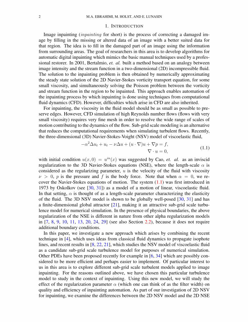
3.1. Stability Behavior of NSE and NSV for Inpainting. In this section we will presenttwo test cases comparing the NSE and NSV both with anisotropic diffusion. The resultspresented here suggests that for some fixed specified time-stepping size dt, the NSVproduced a stable solution in the image inpainting iteration process while the NSE withanisotropic diffusion provided an unstable solution (gray-level blows up). A quick sum-mary of results is provided in Table 1.
For each test cases, we fix the viscosity ν, tolerance tol, and the inpainting region Ω.In Figure 3a, the inpainting region was computed in a grid (in pixels) of 10 × 10. Fordt = 0.1 and ν = 2, the NSE did not converge to the steady state solution due to large
THE NAVIER-STOKES-VOIGHT MODEL FOR IMAGE INPAINTING 9
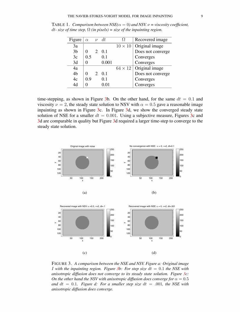
TABLE 1. Comparison between NSE(α = 0) and NSV. ν = viscosity coefficient,dt- size of time step, Ω (in pixels) = size of the inpainting region.
Figure α ν dt Ω Recovered image3a 10× 10 Original image3b 0 2 0.1 Does not converge3c 0.5 0.1 Converges3d 0 0.001 Converges4a 64× 12 Original image4b 0 2 0.1 Does not converge4c 0.9 0.1 Converges4d 0 0.01 Converges
time-stepping, as shown in Figure 3b. On the other hand, for the same dt = 0.1 andviscosity ν = 2, the steady state solution to NSV with α = 0.5 gave a reasonable imageinpainting as shown in Figure 3c. In Figure 3d, we show the converged steady statesolution of NSE for a smaller dt = 0.001. Using a subjective measure, Figures 3c and3d are comparable in quality but Figure 3d required a larger time-step to converge to thesteady state solution.
x
y
Original image with noise
50 100 150 200
20
40
60
80
100
1200
50
100
150
200
250
(a)
x
y
No convergence with NSE: = 0, =2, dt=0.1
50 100 150 200
20
40
60
80
100
1200
50
100
150
200
250
(b)
x
y
Recovered image with NSV: =0.5, =2, dt=.1
50 100 150 200
20
40
60
80
100
1200
50
100
150
200
250
(c)
x
y
Recovered image with NSE: = 0, =2, dt=.001
50 100 150 200
20
40
60
80
100
1200
50
100
150
200
250
(d)
FIGURE 3. A comparison between the NSE and NSV. Figure a: Original imageI with the inpainting region. Figure 3b: For step size dt = 0.1 the NSE withanisotropic diffusion does not converge to its steady state solution. Figure 3c:On the other hand the NSV with anisotropic diffusion does converge for α = 0.5and dt = 0.1. Figure d: For a smaller step size dt = .001, the NSE withanisotropic diffusion does converge.
10 M.A. EBRAHIMI, M. HOLST, AND E. LUNASIN
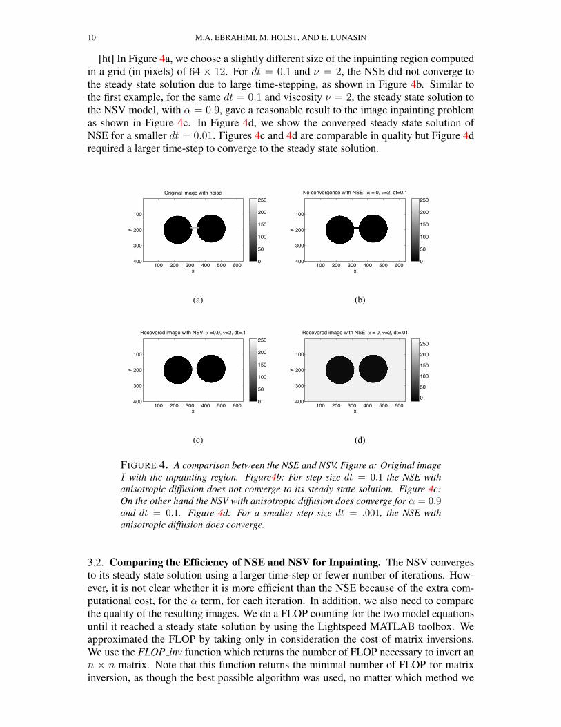
[ht] In Figure 4a, we choose a slightly different size of the inpainting region computedin a grid (in pixels) of 64 × 12. For dt = 0.1 and ν = 2, the NSE did not converge tothe steady state solution due to large time-stepping, as shown in Figure 4b. Similar tothe first example, for the same dt = 0.1 and viscosity ν = 2, the steady state solution tothe NSV model, with α = 0.9, gave a reasonable result to the image inpainting problemas shown in Figure 4c. In Figure 4d, we show the converged steady state solution ofNSE for a smaller dt = 0.01. Figures 4c and 4d are comparable in quality but Figure 4drequired a larger time-step to converge to the steady state solution.
x
y
Original image with noise
100 200 300 400 500 600
100
200
300
400 0
50
100
150
200
250
(a)
x
y
No convergence with NSE: = 0, =2, dt=0.1
100 200 300 400 500 600
100
200
300
400 0
50
100
150
200
250
(b)
x
y
Recovered image with NSV: =0.9, =2, dt=.1
100 200 300 400 500 600
100
200
300
400 0
50
100
150
200
250
(c)
x
y
Recovered image with NSE: = 0, =2, dt=.01
100 200 300 400 500 600
100
200
300
4000
50
100
150
200
250
(d)
FIGURE 4. A comparison between the NSE and NSV. Figure a: Original imageI with the inpainting region. Figure4b: For step size dt = 0.1 the NSE withanisotropic diffusion does not converge to its steady state solution. Figure 4c:On the other hand the NSV with anisotropic diffusion does converge for α = 0.9and dt = 0.1. Figure 4d: For a smaller step size dt = .001, the NSE withanisotropic diffusion does converge.
3.2. Comparing the Efficiency of NSE and NSV for Inpainting. The NSV convergesto its steady state solution using a larger time-step or fewer number of iterations. How-ever, it is not clear whether it is more efficient than the NSE because of the extra com-putational cost, for the α term, for each iteration. In addition, we also need to comparethe quality of the resulting images. We do a FLOP counting for the two model equationsuntil it reached a steady state solution by using the Lightspeed MATLAB toolbox. Weapproximated the FLOP by taking only in consideration the cost of matrix inversions.We use the FLOP inv function which returns the number of FLOP necessary to invert ann × n matrix. Note that this function returns the minimal number of FLOP for matrixinversion, as though the best possible algorithm was used, no matter which method we
THE NAVIER-STOKES-VOIGHT MODEL FOR IMAGE INPAINTING 11
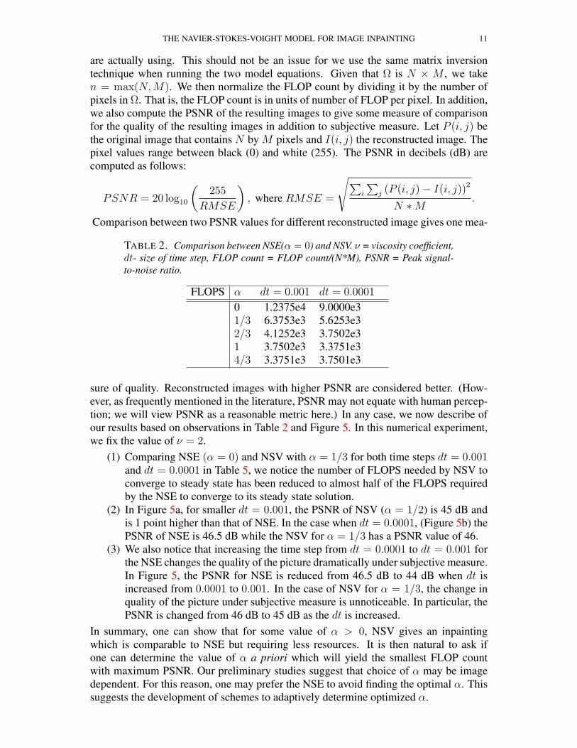
are actually using. This should not be an issue for we use the same matrix inversiontechnique when running the two model equations. Given that Ω is N × M , we taken = max(N,M). We then normalize the FLOP count by dividing it by the number ofpixels in Ω. That is, the FLOP count is in units of number of FLOP per pixel. In addition,we also compute the PSNR of the resulting images to give some measure of comparisonfor the quality of the resulting images in addition to subjective measure. Let P (i, j) bethe original image that contains N by M pixels and I(i, j) the reconstructed image. Thepixel values range between black (0) and white (255). The PSNR in decibels (dB) arecomputed as follows:
PSNR = 20 log10
(255
RMSE
), where RMSE =
√∑i
∑j (P (i, j)− I(i, j))2
N ∗M.
Comparison between two PSNR values for different reconstructed image gives one mea-
TABLE 2. Comparison between NSE(α = 0) and NSV. ν = viscosity coefficient,dt- size of time step, FLOP count = FLOP count/(N*M), PSNR = Peak signal-to-noise ratio.
FLOPS α dt = 0.001 dt = 0.0001
0 1.2375e4 9.0000e31/3 6.3753e3 5.6253e32/3 4.1252e3 3.7502e31 3.7502e3 3.3751e34/3 3.3751e3 3.7501e3
sure of quality. Reconstructed images with higher PSNR are considered better. (How-ever, as frequently mentioned in the literature, PSNR may not equate with human percep-tion; we will view PSNR as a reasonable metric here.) In any case, we now describe ofour results based on observations in Table 2 and Figure 5. In this numerical experiment,we fix the value of ν = 2.
(1) Comparing NSE (α = 0) and NSV with α = 1/3 for both time steps dt = 0.001and dt = 0.0001 in Table 5, we notice the number of FLOPS needed by NSV toconverge to steady state has been reduced to almost half of the FLOPS requiredby the NSE to converge to its steady state solution.
(2) In Figure 5a, for smaller dt = 0.001, the PSNR of NSV (α = 1/2) is 45 dB andis 1 point higher than that of NSE. In the case when dt = 0.0001, (Figure 5b) thePSNR of NSE is 46.5 dB while the NSV for α = 1/3 has a PSNR value of 46.
(3) We also notice that increasing the time step from dt = 0.0001 to dt = 0.001 forthe NSE changes the quality of the picture dramatically under subjective measure.In Figure 5, the PSNR for NSE is reduced from 46.5 dB to 44 dB when dt isincreased from 0.0001 to 0.001. In the case of NSV for α = 1/3, the change inquality of the picture under subjective measure is unnoticeable. In particular, thePSNR is changed from 46 dB to 45 dB as the dt is increased.
In summary, one can show that for some value of α > 0, NSV gives an inpaintingwhich is comparable to NSE but requiring less resources. It is then natural to ask ifone can determine the value of α a priori which will yield the smallest FLOP countwith maximum PSNR. Our preliminary studies suggest that choice of α may be imagedependent. For this reason, one may prefer the NSE to avoid finding the optimal α. Thissuggests the development of schemes to adaptively determine optimized α.

12 M.A. EBRAHIMI, M. HOLST, AND E. LUNASIN
0 5 10 15 20 25 30 3542
43
44
45
46
47
no. of frames (iterations)
PSN
R
dt = 0.001
a. NSE ( =2)b. NSV ( =1/3, =2)c. NSV ( =2/3, =2)d. NSV ( =1, =2)e. NSV ( =4/3, =2)f. NSV ( =5/3, =2)g. NSV ( =62, =2)
(a)
5 10 15 20 25 30 3542
43
44
45
46
47
no. of frames (iterations)
PSN
R
dt = 0.0001
a. NSE ( =2)b. NSV ( =1/3, =2)c. NSV ( =2/3, =2)d. NSV ( =1, =2)e. NSV ( =4/3, =2)f. NSV ( =5/3, =2)g. NSV ( =62, =2)
(b)
FIGURE 5. PSNR of NSE vs NSV (for various values of α). When dt = 0.001,the PSNR of NSV (α=1/3) is higher than the NSE and requires only about half ofthe number of FLOPS needed for the NSE to converge to its steady state solution.
x
y
Recovered Image = 0
50 100 150 200 250
50
100
150
200
25040
60
80
100
120
140
160
180
200
220
(a)
x
y
Recovered Image = 1/3
50 100 150 200 250
50
100
150
200
25040
60
80
100
120
140
160
180
200
220
(b)
FIGURE 6. An example of image recovered for (a) NSE and (b) NSV (α = 1/3)with dt = 0.0001.
4. SOME SUPPORTING THEORETICAL RESULTS
In this section we summarize some existing results, and then establish some new re-sults that support the numerical results in the previous section. To this end, let Ω =[0, 2πL]2. The NSE of viscous incompressible flows, subject to periodic boundary con-dition on domain Ω, is written in the form:
∂tu− ν∆u+ (u · ∇)u = −∇p+ f,
∇ · u = 0,(4.1)
THE NAVIER-STOKES-VOIGHT MODEL FOR IMAGE INPAINTING 13
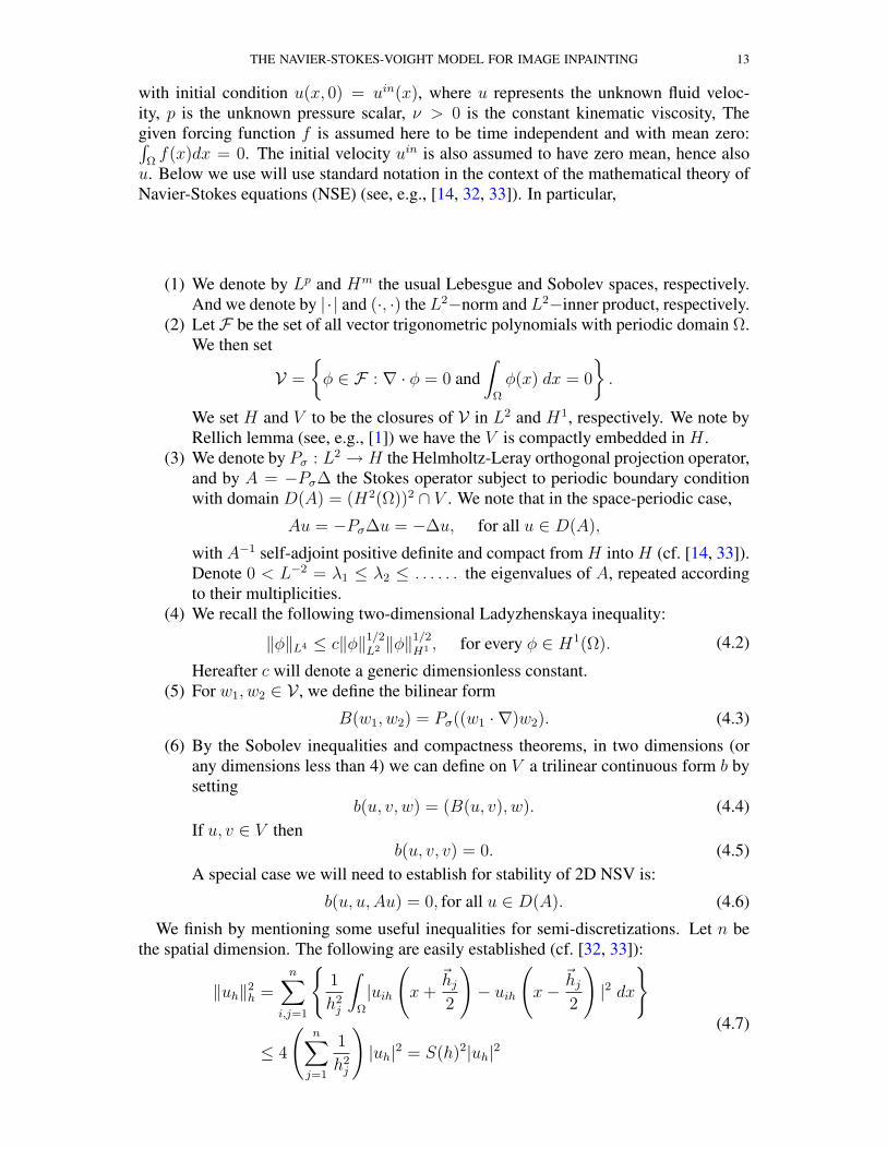
with initial condition u(x, 0) = uin(x), where u represents the unknown fluid veloc-ity, p is the unknown pressure scalar, ν > 0 is the constant kinematic viscosity, Thegiven forcing function f is assumed here to be time independent and with mean zero:∫
Ωf(x)dx = 0. The initial velocity uin is also assumed to have zero mean, hence also
u. Below we use will use standard notation in the context of the mathematical theory ofNavier-Stokes equations (NSE) (see, e.g., [14, 32, 33]). In particular,
(1) We denote by Lp and Hm the usual Lebesgue and Sobolev spaces, respectively.And we denote by | · | and (·, ·) the L2−norm and L2−inner product, respectively.
(2) Let F be the set of all vector trigonometric polynomials with periodic domain Ω.We then set
V =
φ ∈ F : ∇ · φ = 0 and
∫Ω
φ(x) dx = 0
.
We set H and V to be the closures of V in L2 and H1, respectively. We note byRellich lemma (see, e.g., [1]) we have the V is compactly embedded in H .
(3) We denote by Pσ : L2 → H the Helmholtz-Leray orthogonal projection operator,and by A = −Pσ∆ the Stokes operator subject to periodic boundary conditionwith domain D(A) = (H2(Ω))2 ∩ V . We note that in the space-periodic case,
Au = −Pσ∆u = −∆u, for all u ∈ D(A),
with A−1 self-adjoint positive definite and compact from H into H (cf. [14, 33]).Denote 0 < L−2 = λ1 ≤ λ2 ≤ . . . . . . the eigenvalues of A, repeated accordingto their multiplicities.
(4) We recall the following two-dimensional Ladyzhenskaya inequality:
‖φ‖L4 ≤ c‖φ‖1/2
L2 ‖φ‖1/2
H1 , for every φ ∈ H1(Ω). (4.2)
Hereafter c will denote a generic dimensionless constant.(5) For w1, w2 ∈ V , we define the bilinear form
B(w1, w2) = Pσ((w1 · ∇)w2). (4.3)
(6) By the Sobolev inequalities and compactness theorems, in two dimensions (orany dimensions less than 4) we can define on V a trilinear continuous form b bysetting
b(u, v, w) = (B(u, v), w). (4.4)If u, v ∈ V then
b(u, v, v) = 0. (4.5)A special case we will need to establish for stability of 2D NSV is:
b(u, u,Au) = 0, for all u ∈ D(A). (4.6)
We finish by mentioning some useful inequalities for semi-discretizations. Let n bethe spatial dimension. The following are easily established (cf. [32, 33]):
‖uh‖2h =
n∑i,j=1
1
h2j
∫Ω
|uih
(x+
~hj2
)− uih
(x−
~hj2
)|2 dx
≤ 4
(n∑j=1
1
h2j
)|uh|2 = S(h)2|uh|2
(4.7)
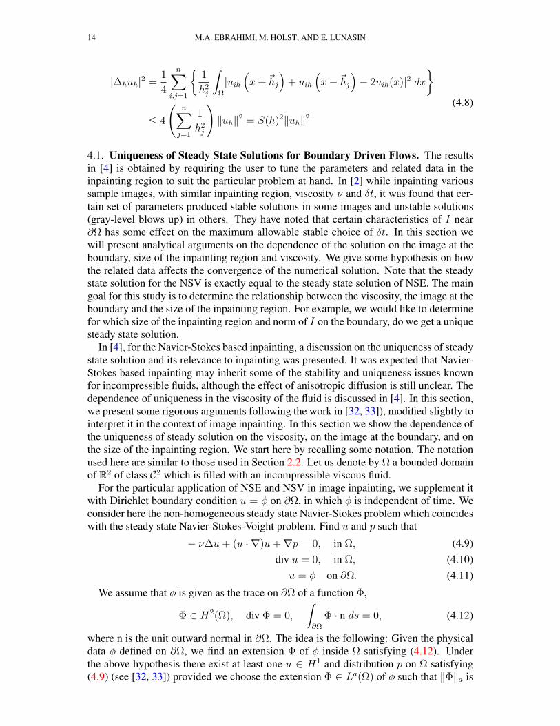
14 M.A. EBRAHIMI, M. HOLST, AND E. LUNASIN
|∆huh|2 =1
4
n∑i,j=1
1
h2j
∫Ω
|uih(x+ ~hj
)+ uih
(x− ~hj
)− 2uih(x)|2 dx
≤ 4
(n∑j=1
1
h2j
)‖uh‖2 = S(h)2‖uh‖2
(4.8)
4.1. Uniqueness of Steady State Solutions for Boundary Driven Flows. The resultsin [4] is obtained by requiring the user to tune the parameters and related data in theinpainting region to suit the particular problem at hand. In [2] while inpainting varioussample images, with similar inpainting region, viscosity ν and δt, it was found that cer-tain set of parameters produced stable solutions in some images and unstable solutions(gray-level blows up) in others. They have noted that certain characteristics of I near∂Ω has some effect on the maximum allowable stable choice of δt. In this section wewill present analytical arguments on the dependence of the solution on the image at theboundary, size of the inpainting region and viscosity. We give some hypothesis on howthe related data affects the convergence of the numerical solution. Note that the steadystate solution for the NSV is exactly equal to the steady state solution of NSE. The maingoal for this study is to determine the relationship between the viscosity, the image at theboundary and the size of the inpainting region. For example, we would like to determinefor which size of the inpainting region and norm of I on the boundary, do we get a uniquesteady state solution.
In [4], for the Navier-Stokes based inpainting, a discussion on the uniqueness of steadystate solution and its relevance to inpainting was presented. It was expected that Navier-Stokes based inpainting may inherit some of the stability and uniqueness issues knownfor incompressible fluids, although the effect of anisotropic diffusion is still unclear. Thedependence of uniqueness in the viscosity of the fluid is discussed in [4]. In this section,we present some rigorous arguments following the work in [32, 33]), modified slightly tointerpret it in the context of image inpainting. In this section we show the dependence ofthe uniqueness of steady solution on the viscosity, on the image at the boundary, and onthe size of the inpainting region. We start here by recalling some notation. The notationused here are similar to those used in Section 2.2. Let us denote by Ω a bounded domainof R2 of class C2 which is filled with an incompressible viscous fluid.
For the particular application of NSE and NSV in image inpainting, we supplement itwith Dirichlet boundary condition u = φ on ∂Ω, in which φ is independent of time. Weconsider here the non-homogeneous steady state Navier-Stokes problem which coincideswith the steady state Navier-Stokes-Voight problem. Find u and p such that
− ν∆u+ (u · ∇)u+∇p = 0, in Ω, (4.9)div u = 0, in Ω, (4.10)u = φ on ∂Ω. (4.11)
We assume that φ is given as the trace on ∂Ω of a function Φ,
Φ ∈ H2(Ω), div Φ = 0,
∫∂Ω
Φ · n ds = 0, (4.12)
where n is the unit outward normal in ∂Ω. The idea is the following: Given the physicaldata φ defined on ∂Ω, we find an extension Φ of φ inside Ω satisfying (4.12). Underthe above hypothesis there exist at least one u ∈ H1 and distribution p on Ω satisfying(4.9) (see [32, 33]) provided we choose the extension Φ ∈ La(Ω) of φ such that ‖Φ‖a is
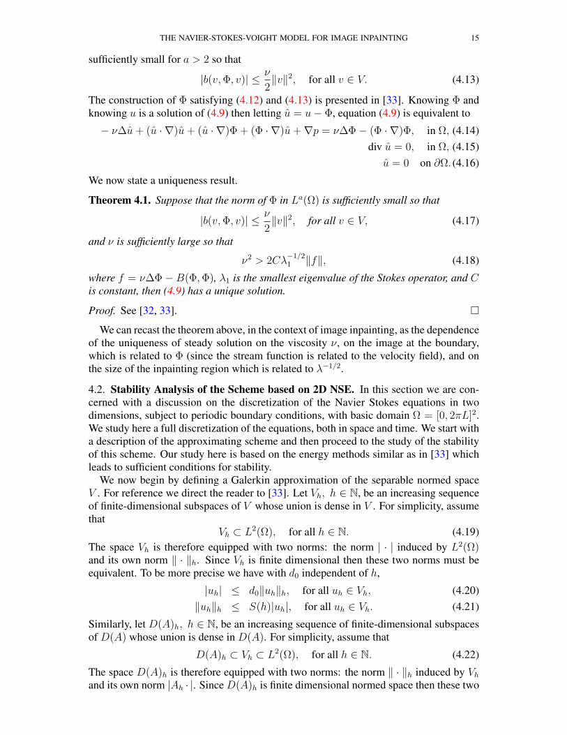
THE NAVIER-STOKES-VOIGHT MODEL FOR IMAGE INPAINTING 15
sufficiently small for a > 2 so that
|b(v,Φ, v)| ≤ ν
2‖v‖2, for all v ∈ V. (4.13)
The construction of Φ satisfying (4.12) and (4.13) is presented in [33]. Knowing Φ andknowing u is a solution of (4.9) then letting u = u− Φ, equation (4.9) is equivalent to
− ν∆u+ (u · ∇)u+ (u · ∇)Φ + (Φ · ∇)u+∇p = ν∆Φ− (Φ · ∇)Φ, in Ω, (4.14)div u = 0, in Ω, (4.15)
u = 0 on ∂Ω. (4.16)
We now state a uniqueness result.
Theorem 4.1. Suppose that the norm of Φ in La(Ω) is sufficiently small so that
|b(v,Φ, v)| ≤ ν
2‖v‖2, for all v ∈ V, (4.17)
and ν is sufficiently large so that
ν2 > 2Cλ−1/21 ‖f‖, (4.18)
where f = ν∆Φ− B(Φ,Φ), λ1 is the smallest eigenvalue of the Stokes operator, and Cis constant, then (4.9) has a unique solution.
Proof. See [32, 33].
We can recast the theorem above, in the context of image inpainting, as the dependenceof the uniqueness of steady solution on the viscosity ν, on the image at the boundary,which is related to Φ (since the stream function is related to the velocity field), and onthe size of the inpainting region which is related to λ−1/2.
4.2. Stability Analysis of the Scheme based on 2D NSE. In this section we are con-cerned with a discussion on the discretization of the Navier Stokes equations in twodimensions, subject to periodic boundary conditions, with basic domain Ω = [0, 2πL]2.We study here a full discretization of the equations, both in space and time. We start witha description of the approximating scheme and then proceed to the study of the stabilityof this scheme. Our study here is based on the energy methods similar as in [33] whichleads to sufficient conditions for stability.
We now begin by defining a Galerkin approximation of the separable normed spaceV . For reference we direct the reader to [33]. Let Vh, h ∈ N, be an increasing sequenceof finite-dimensional subspaces of V whose union is dense in V . For simplicity, assumethat
Vh ⊂ L2(Ω), for all h ∈ N. (4.19)The space Vh is therefore equipped with two norms: the norm | · | induced by L2(Ω)and its own norm ‖ · ‖h. Since Vh is finite dimensional then these two norms must beequivalent. To be more precise we have with d0 independent of h,
|uh| ≤ d0‖uh‖h, for all uh ∈ Vh, (4.20)‖uh‖h ≤ S(h)|uh|, for all uh ∈ Vh. (4.21)
Similarly, let D(A)h, h ∈ N, be an increasing sequence of finite-dimensional subspacesof D(A) whose union is dense in D(A). For simplicity, assume that
D(A)h ⊂ Vh ⊂ L2(Ω), for all h ∈ N. (4.22)
The space D(A)h is therefore equipped with two norms: the norm ‖ · ‖h induced by Vhand its own norm |Ah · |. Since D(A)h is finite dimensional normed space then these two
16 M.A. EBRAHIMI, M. HOLST, AND E. LUNASIN
norms must be equivalent. To be more precise we have with d2 independent of h,
‖uh‖h ≤ d2|Ahuh|, for all uh ∈ D(A)h, (4.23)|Ahuh| ≤ cS(h)‖uh‖h, for all uh ∈ D(A)h. (4.24)
The constant S(h), which depends on h is sometimes called the stability constant sinceit plays a major important role in obtaining necessary conditions on the stability of nu-merical approximations. Usually S(h)→∞, as h→ 0.
Let there be given a trilinear continuous form on Vh, say bh(uh, vh, wh) which satisfiesthe following:
(1) For all uh, vh ∈ Vh, both of the following hold:
bh(uh, vh, vh) = 0, (4.25)
|bh(uh, uh, vh)| ≤ d1‖uh‖2h‖vh‖h ≤ d1S
2(h)|uh|‖uh‖h|vh|≤ S1(h)|uh|‖uh‖h|vh|,
(4.26)
where at least,S1(h) ≤ d1S
2(h). (4.27)(2) For all uh, vh, wh ∈ Vh,
|bh(uh, vh, wh)| ≤ d1‖uh‖h‖vh‖h‖wh‖h. (4.28)
We divide the interval [0, T ] into N intervals of equal length k = T/N . We associatewith k and the function f , the elements f1, . . . , f
N :
fm =1
k
∫ mk
(m−1)k
f(t) dt, m = 1, . . . , N ; fm ∈ L2(Ω). (4.29)
We denote by u0h the orthogonal projection of the initial condition u0 onto D(A)h in
L2(Ω). When u0h, . . . , u
m−1h , are known, umh is the solution in D(A)h of
1
k(umh − um−1
h , vh) + ν((um−1h , vh))h + bh(u
m−1h , um−1
h , vh) = (fm, vh) (4.30)
for all vh ∈ D(A)h.
Lemma 4.2. We assume that k and h satisfy
(1) kS2(h) ≤ 1− δ4ν
for some δ, 0 < δ < 1 ,
(2) kS2(h) ≤ 1,
(3) kS21(h)S2(h) ≤ νδ
8d20d5
,
where d0 is as in (4.20) and
d5 = ‖u0‖2 + d20
(d2
0 + 1− δνd2
0
)∫ T
0
|f(s)|2 ds, (4.31)
then, the umh given by (4.30) remain bounded in the following sense
‖umh ‖2h ≤ d5 m = 1, . . . , N, (4.32)
k
r∑m=1
|Ahum−1h |2 ≤ 2d5
νδ, (4.33)
N∑m=1
‖umh − um−1h ‖2
h ≤ 2
(2− δδ
)d5 + 4
∫ T
0
|f(s)|2 ds. (4.34)
THE NAVIER-STOKES-VOIGHT MODEL FOR IMAGE INPAINTING 17
Proof. We replace by vh by Ahum−1h in (4.30); due to the identity
2(a− b, b) = |a|2 − |b|2 − |a− b|2, (4.35)
we find‖umh ‖2
h − ‖um−1h ‖2
h − ‖umh − um−1h ‖2
h + 2kν|Ahum−1h |2 = 2k(fm, Ahu
m−1h )
≤ 2kd0|fm||Ahum−1h |
≤ kν|Ahum−1h |2 + k
d20
ν|fm|2.
(4.36)
We would like to majorize ‖umh −um−1h ‖2
h in (4.36). Let vh = Ahumh −Ahum−1
h in (4.30).This gives
2‖umh − um−1h ‖2
h = −2kν(Ahu
m−1h , A(umh − um−1
h ))
− 2kbh(um−1h , um−1
h , Ahumh − um−1
h )
+ 2k(fm, Ah(umh − um−1
h )) =: I1 + I2 + I3.
(4.37)
We successively majorize I1, I2 and I3 using (4.21), (4.24), (4.26), and Cauchy-Schwarzinequality
|I1| ≤ 2kν|Ahum−1h ||Ah(umh − um−1
h )| (4.38)≤ 2kνS(h)|Ahum−1
h |‖umh − um−1h ‖h (4.39)
≤ 1
4‖umh − um−1
h ‖2h + 4k2ν2S2(h)|Ahum−1
h |2, (4.40)
|I2| ≤ 2kS1(h)|um−1h |‖um−1
h ‖h|Ah(umh − um−1h )| (4.41)
≤ 2kS(h)S1(h)|um−1h |‖um−1
h ‖h‖umh um−1h ‖h (4.42)
≤ 1
4‖umh − um−1
h ‖2h + 4k2d0S
2(h)S21(h)|um−1
h |2‖um−1h ‖2
h (4.43)
≤ 1
4‖umh − um−1
h ‖2h + 4k2d2
0S2(h)S2
1(h)|um−1h |2|Ahum−1
h |2, (4.44)
|I3| ≤ 2k|fm||Ah(umh − um−1h )| ≤ 2kS(h)|fm|‖umh − um−1
h ‖h (4.45)
≤ 1
4‖umh − um−1
h ‖2h + 4k2S2(h)|fm|. (4.46)
Denoting as Θ = 4k2d20S
21(h)S2(h)|um−1
h |2|Ahum−1h |2, we have that (4.37) becomes
‖umh − um−1h ‖2
h ≤ 4k2ν2S(h)|Ahum−1h |2 + Θ ≤ kν(1− δ)|Ahum−1
h |2 + Θ. (4.47)
Going back to (4.36) we have
‖umh ‖2h − ‖um−1
h ‖2h + k(νδ − 4kd2
0S21(h)S2(h)|um−1
h |2)|Ahum−1h |2
≤ k
(d2
0
ν+ 4kS2(h)
)|fm|2
≤ kd20
(1
ν+
1− δνd2
0
)|fm|2
≤ kd20
(d2
0 + 1− δνd2
0
)|fm|2.
(4.48)
18 M.A. EBRAHIMI, M. HOLST, AND E. LUNASIN
Summing up (4.48) for m = 1 to r we get
‖urh‖2h + k
r∑m=1
(νδ − 4kd2
0S21(h)S2(h)|um−1
h |2)|Ahum−1
h |2 ≤ µr, (4.49)
where
µr = ‖u0h‖2
h + kd20
(d2
0 + 1− δνd2
0
) r∑m=1
|fm|2.
Now using condition (iii) in Lemma 4.2, we will prove by the method of induction that
‖urh‖2h +
kνδ
2
r∑m=1
|Ahum−1h |2 ≤ µr, r = 1 to N. (4.50)
First observe that
µr ≤ µN = ‖u0h‖2 + kd2
0
(d2
0 + 1− δνd2
0
) N∑m−1
|fm|2
≤ ‖u0‖2 + d20
(d2
0 + 1− δνd2
0
)∫ T
0
|f(s)|2 ds =: d5
(4.51)
To establish the basis for induction (r = 1) we write (4.48) for m = 1 and use (iii) inLemma 4.2 to get
‖u1h‖2
h + kνδ|Ahu0h|2 ≤ ‖u0
h‖2h + 4k2d2
0S21(h)S2(h)|u0
h|2|Ahu0h|2
+ kd20
(d2
0 + 1− δνd2
0
)|f 1|2
≤ µ1 +kνδ
2|Ahu0
h|2.
(4.52)
Thus equation (4.50) for r = 1 is satisfied. By induction on r, assume that (4.50) holdsup to the order r − 1. Note that by the recurrence hypothesis
‖ur−1h ‖
2h ≤ µr−1 ≤ µN ≤ d5. (4.53)
Thus by (4.49), we have
‖urh‖2h + kνδ
r∑m=1
|Ahum−1h |2 ≤ µr + 4k2d2
0S21(h)S2(h)|um−1
h |2
≤ µr + 4k2d20S
21(h)S2(h)d5
r∑m=1
|Ahum−1h |2
≤ µ2 +kνδ
2
r∑m=1
|Ahum−1h |2.
(4.54)
Hence,
‖urh‖2h +
kνδ
2
r∑m=1
|Ahum−1h |2 ≤ µr. (4.55)

THE NAVIER-STOKES-VOIGHT MODEL FOR IMAGE INPAINTING 19
This gives (4.33). It remains to prove (4.34). From (4.47), applying (ii) and (iii) fromLemma 4.2, we get
‖umh − um−1h ‖2
h ≤ k2ν2S(h)|Ahum−1h |2 + 4k2d2
0S21(h)S2(h)|um−1
h |2|Ahuhm− 1|2
+ 4k2S2(h)|fm|2
≤ kν(1− δ)|Ahum−1h |2 + 4k
νδ
8d5
|um−1h |2|Ahum−1
h |2 + 4k|fm|2
≤ kν(1− δ)|Ahum−1h |2 + kνδ|Ahum−1
h |2 + 4k|fm|2
≤ kν(2− δ)|Ahum−1h |2 + 4k|fm|2.
(4.56)Summing it up over all m = 1 to N and using (4.33) we find (4.34).
4.3. Stability Analysis of the Scheme based on 2D NSV. The preliminary setup is thesame as those of 2D NSE in the previous section. When u0
h, . . . , um−1h , are known, umh is
the solution in D(A)h of
1
k(umh − um−1
h , vh) +α2
k
(Ahu
mh − Ahum−1
h , vh)
+ ν((um−1h , vh))h
+bh(um−1h , um−1
h , vh) = (fm, vh),(4.57)
for all vh ∈ Vh.
Lemma 4.3. We assume that k and h satisfy
(1) kS2(h) ≤ 1− δ4ν
for some δ, 0 < δ < 1,
(2) kS21(h) ≤ νδ
8d6
,
d6 = |u0|2 + α2‖u0‖2 +
(d2
0
ν+ 4T
)∫ T
0
|f(s)|2 ds, (4.58)
and d0 is as in (4.20), then, the umh given by (4.57) remain bounded in the following sense
|umh |2 + α2‖umh ‖2h ≤ d6 m = 1, . . . , N, (4.59)
k
r∑m=1
‖um−1h ‖2
h ≤2d6
νδ, (4.60)
N∑m=1
(|umh − um−1
h |2 + α2‖umh − um−1h ‖2
h
)≤(
2− δδ
)d6 + 4T
∫ T
0
|f(s)|2 ds. (4.61)
Proof. We replace by vh by um−1h in (4.57); due to (4.20), (4.21),(4.35) and Cauchy-
Schwarz, we get
|umh |2 − |um−1h |2 − |umh − um−1
h |2 + 2kν‖um−1h ‖2
h
+ α2(‖umh ‖2
h − ‖um−1h ‖2
h − ‖umh − um−1h ‖2
h
)= 2k(fm, Ahu
m−1h )
≤ 2kd0|fm|‖um−1h ‖h ≤ kν‖um−1
h ‖2h + k
d20
ν|fm|2,
(4.62)
20 M.A. EBRAHIMI, M. HOLST, AND E. LUNASIN
that is, (|umh |2 − |um−1
h |2)
+ α2(‖umh ‖2
h − ‖um−1h ‖2
h
)−(|umh − um−1
h |2 + α2‖umh − um−1h ‖2
h
)≤ k
d20
ν|fm|2.
(4.63)
We would like to majorize the term(|umh − um−1
h |2 + α2‖umh − um−1h ‖2
h
)in (4.63). Let
vh = umh − um−1h in (4.57). This gives
2|umh − um−1h |2 + 2α2‖umh − um−1
h ‖2h
= −2kν((um−1h , umh − um−1
h
))h
− 2kbh(um−1h , um−1
h , umh − um−1h ) + 2k(fm, umh − um−1
h ) =: I1 + I2 + I3.
(4.64)
We successively majorize I1, I2 and I3 using repeatedly (4.21), (4.26), and Cauchy-Schwarz inequality and get exactly the estimates as in page 234 of [33]. Therefore (4.64)becomes|umh − um−1
h |2 + α2‖umh − um−1h ‖2
h ≤ 4k2ν2S(h)‖um−1h ‖2
h
+ 4k2S21(h)|um−1
h |2‖um−1h ‖2
h + 4k2|fm|2
≤ kν(1− δ)‖um−1h ‖2
h
+ 4k2S21(h)|um−1
h |2‖um−1h ‖2
h + 4k2|fm|2.
(4.65)
Going back to (4.63) we have
|umh |2 − |um−1h |2 + α2
(‖umh ‖2
h − ‖um−1h ‖2
h
)+ k(νδ − 4kS2
1(h)|um−1h |2)‖um−1
h ‖2h
≤ k
(d2
0
ν+ 4k
)|fm|2
≤ k
(d2
0
ν+ 4T
)|fm|2 (since k ≤ T ).
(4.66)
Summing up (4.65) for m = 1 to r we get
|urh|2 + α2‖urh‖2h + k
r∑m=1
(νδ − 4kS2
1(h)|um−1h |2
)‖um−1
h ‖2h ≤ µr, (4.67)
where
µr = |u0h|2 + α2‖u0
h‖2h + k
(d2
0
ν+ 4T
) r∑m=1
|fm|2.
Now using condition (ii) in Lemma 4.3, we will prove by the method of induction that
|urh|2 + α2‖urh‖2h +
kνδ
2
r∑m=1
‖um−1h ‖2
h ≤ µr, r = 1 to N. (4.68)
First observe that
µr ≤ µN = |u0h|2 + α2‖u0
h‖2 + k
(d2
0
ν+ 4T
) N∑m−1
|fm|2 =: d6. (4.69)

THE NAVIER-STOKES-VOIGHT MODEL FOR IMAGE INPAINTING 21
To establish the basis for induction (r = 1) we write (4.66) for m = 1 and use (ii) inLemma 4.3 to get
|u1h|2 + α2‖u1
h‖2h + kνδ‖u0
h‖2h ≤ |u0
h|2 + α2‖u0h‖2
h,
+ 4k2S21(h)|u0
h|2‖u0h‖2
h + k
(d2
0
ν+ 4T
)|f 1|2 ≤ µ1 +
kνδ
2‖u0
h‖2h.
(4.70)
Thus equation (4.68) for r = 1 is satisfied. By induction on r, assume that (4.68) holdsup to the order r − 1. Note that by the recurrence hypothesis
|ur−1h |
2 + α2‖ur−1h ‖
2h ≤ µr−1 ≤ µN ≤ d6. (4.71)
Thus by (4.67), we have
|ur−1h |
2 + α2‖urh‖2h + kνδ
r∑m=1
‖um−1h ‖2
h ≤ µr + 4k2S21(h)|um−1
h |2|um−1h |2
≤ µr + 4k2S21(h)d6
r∑m=1
‖um−1h ‖2
h
≤ µ2 +kνδ
2
r∑m=1
‖um−1h ‖2
h.
(4.72)
Hence,
|urh|2 + α2‖urh‖2h +
kνδ
2
r∑m=1
‖um−1h ‖2
h ≤ µr. (4.73)
This gives us (4.60). It remains to prove (4.61). From (4.65) and applying condition (i)and (ii) from Lemma 4.3, we get
|umh − um−1h |2 + α2‖umh − um−1
h ‖2h ≤ kν(1− δ)‖um−1
h ‖2h
+ 4k2S21(h)|um−1
h |2‖um−1h ‖2
h + 4k2|fm|2
≤ kν
(1− δ
2
)‖um−1
h ‖2h + 4kT |fm|2.
(4.74)
Summing it up over all m = 1 to N and using (4.60) we find (4.61).
4.4. Stability Analysis of a Semi-Implicit Scheme based on 2D NSE. We presenthere general results for stability analysis for the full NSE equations vorticity formula-tion (implicit only on the linear part of the operator). The setup is as follows: Whenu0h, . . . , u
m−1h , are known, umh is the solution in D(A)h of
1
k(umh − um−1
h , vh) + ν((umh , vh))h + bh(um−1h , um−1
h , vh) = (fm, vh), (4.75)
for all vh ∈ Vh.
Lemma 4.4. We assume that k and h satisfy
(1) kS4(h) ≤ d′,(2) kS2
1(h)S2(h) ≤ d′′,
where d′ = and d′′ =, then, the umh given by (4.75) remain bounded in the following sense
‖umh ‖h ≤ d7, m = 0, . . . , N,
N∑m=1
‖umh − um−1h ‖2
h ≤ d7, kN∑m=1
|Ahumh |2 ≤ d7,(4.76)
22 M.A. EBRAHIMI, M. HOLST, AND E. LUNASIN
where d7 is some constant depending only on the data d′ and d′′.
Proof. We let vh = Ahumh in (4.75). Using the identity (4.35), we get
‖umh ‖2h − ‖um−1
h ‖h + ‖umh − um−1h ‖2
h + 2kν|Ahumh |2
= −2kbh(um−1h , um−1
h , Ahumh
)+ 2k(fm, Ahu
mh )
:= I1 + I2.
(4.77)
We would like bound the terms I1 and I2. The identity bh(um−1h , um−1
h , Aum−1h
)= 0
together with (4.20) and (4.26) gives
|I1| ≤ 2kS1(h)|um−1h |‖um−1
h ‖h|A(umh − um−1h )|
≤ 2kS1(h)S(h)|um−1h |‖um−1
h ‖h‖umh − um−1h ‖h
≤ 2k2S21(h)S2(h)|um−1
h |2‖um−1h ‖2
h +1
2‖umh − um−1
h ‖h,(4.78)
and
|I2| ≤ 2kd0|fm||Ahumh | ≤ k
(d2
0
ν|fm|2 + ν|Aumh |2
). (4.79)
Hence,
‖umh ‖2h − ‖um−1
h ‖2h +
1
2‖umh − um−1
h ‖2h + kν|Ahumh |2
− 2k2S21(h)S2(h)|um−1
h |2‖um−1h ‖2
h ≤kd2
0
ν|fm|2.
(4.80)
We sum up these inequalities for m = 1 to r, to get
‖urh‖2h +
1
2
r∑m=1
‖umh − um−1h ‖2
h + kν
r∑m=1
|Ahumh |2
− 2k2S21(h)S2(h)
r∑m=2
|um−1h |2‖um−1
h ‖2h ≤ λr,
(4.81)
where,
λr = ‖u0h‖h =
kd20
ν
r∑m=1
|fm|2 + 2k2S21(h)S2(h)|u0
h|2‖u0h‖2
h. (4.82)
We assume that2kd0d2S
21(h)S2(h)λN ≤ ν − δ, (4.83)
for some fixed δ, 0 ≤ δ ≤ ν. If this holds then one can show recursively that
‖urh‖2h +
1
2
r∑m−1
‖umh − um−1h ‖2
h + kδr∑
m=1
|Ahumh |2 ≤ λr, r = 1, . . . , N. (4.84)
Clearly, letting m = 1 in (4.80) shows that (4.84) is true for r = 1. Let us assume that(4.84) is valid up to the order r − 1, we want to show that (4.84) is valid for r. Observe
THE NAVIER-STOKES-VOIGHT MODEL FOR IMAGE INPAINTING 23
that by the inductive hypothesis ‖umh ‖2h ≤ λm ≤ λN . Hence, by the condition (4.83)
2k2S21(h)S2(h)
r∑m=2
|um−1h |‖um−1
h ‖2h ≤ 2d2k
2S21(h)S2(h)
r∑m=2
|um−1h ||Ahum−1
h |2
≤ 2d0d2k2S2
1(h)S2(h)λN
r∑m−1
|Ahum−1h |2
≤ k(ν − δ)r∑
m=1
|Ahum−1h |2.
(4.85)
We apply this upper bound into (4.81), we get (4.84) for the integer r. To complete theproof it suffices to show that conditions (i) and (ii) in Lemma 4.4 ensure the condition(4.83). We recall that since ‖u0
h‖ ≤ ‖u0‖ for all h and
k
N∑m=1
|fm|2 ≤∫ T
0
|f(s)|2 ds,
then,
λN ≤ ‖u0‖2 +d2
0
ν
∫ T
0
||f(s)|2 ds+ 2k2S21(h)S2(h)|u0|2‖u0
h‖2h
≤ d10 + 2k2S21(h)S2(h)|u0|2‖u0‖2.
(4.86)
Hence, if kS21S
2(h) ≤ d′, then
2kd0d2S21(h)S2(h)λN ≤ 2d′(d10 + 2d′d′′|u0|2‖u0‖2) ≤ ν − δ, (4.87)
provided d′, d′′ are sufficiently small.
5. SUMMARY
The NSV model of viscoelastic incompressible fluid has been proposed as a regular-ization of the 3D NSE for purposes of direct numerical simulation. In this work, we haveshown one of the benefits of using the 2D NSV turbulence model for small regularizationparameter α, instead of the 2D NSE to reduce computational expense when automatingthe inpainting process. To be more precise, one can find a parameter α > 0 in whichthe 2D NSV gives a solution to the image inpainting problem comparable (both usingsubjective and objective measure) to that of the solution of the 2D NSE but only requiresa time step much larger in comparison to that of 2D NSE. That is, the 2D NSV convergeto the steady state solution with a much larger time step and hence solves the image in-painting problem using less computational resources. In the numerical experiments, wefound that after accounting for the relative costs of the two methods, the 2D NSV givesa solution to the inpainting problem which matches the quality of the image produced bywhen NSE is used but using less resources.
In future work we would like to investigate other PDEs which can be used instead ofthe 2D NSE and 2D NSV when solving the inpainting process. In particular, we wouldlike to use a PDE to solve the inpainting problem without the addition of anisotropicdiffusion. The dependence of the stability of solutions on certain characteristics of theimage near the boundary is also of major interest in this topic. We would like to in-vestigate the dependence of the uniqueness of steady solution on the viscosity, on theimage at the boundary, and on the size of the inpainting region. We have presented somebasic results on the uniqueness of steady state solution of the 2D steady state applied in
24 M.A. EBRAHIMI, M. HOLST, AND E. LUNASIN
the context of image inpainting. We would like to do further numerical experiments toverify these hypothesis.
6. ACKNOWLEDGMENTS
We would like to thank E.S. Titi, D. Reynolds, and Y. Zhou for valuable discussionson discretization techniques and other helpful comments on this study. In particular, wewould like to thank E.S. Titi for showing us the proof of the dependence of the uniquenessof the inpainting solution on the viscosity, on the image at the boundary and the size ofinpainting region. MH was supported in part by NSF Awards 0715146 and 0915220. MEand EL were supported in part by NSF Award 0715146.
REFERENCES
[1] R. ADAMS, Compact imbeddings of Wm,p(Ω), in Sobolev Spaces, S. Eilenberg and H. Bass, eds.,Academic Press, New York, 1975.
[2] W. AU AND R. TAKEI, Image inpainting with the Navier-Stokes equations. Available at Final ReportAPMA 930 SFU, 2002.
[3] C. BARDOS, J. LINSHIZ, AND E. S. TITI, Global regularity for a Birkhoff-Rott-α approximation ofthe dynamics of vortex sheets of the 2D Euler equations. 2008.
[4] M. BERTALMIO, A. L. BERTOZZI, AND G. SAPIRO, Navier-Stokes, fluid dynamics, and imageand video inpainting, 2001 I E E E Computer Society Conference on Computer Vision and PatternRecognition (CVPR’01), 1 (2001), p. 35.
[5] M. BERTALMIO, G. SAPIRO, V. CASELLES, AND C. BALLESTER, Image inpainting, InternationalConference on Computer Graphics and Interactive Techniques, (2000), pp. 417–424.
[6] F. BORNEMANN AND T. MARZ, Fast image inpainting based on coherence transport, J. Math,Imaging Vis., 28 (2007), pp. 259–278.
[7] C. CAO, D. HOLM, AND E. TITI, On the Clark-α model of turbulence: global regularity andlong-time dynamics, Journal of Turbulence, 6 (2005), pp. 1–11.
[8] Y. CAO, E. LUNASIN, AND E. TITI, Global well-posedness of the viscous and inviscid simplifiedBardina model, Communications in Mathematical Sciences, 4 (2006), pp. 823–848.
[9] S. CHEN, C. FOIAS, D. HOLM, E. OLSON, E. TITI, AND S. WYNNE, Camassa–Holm equationsas closure model for turbulent channel and pipe flow, Phys. Rev. Lett., 81 (1998), pp. 5338–5341.
[10] , The Camassa–Holm equations and turbulence, Phys. D, 133 (1999), pp. 49–65.[11] , A connection between the Camassa-Holm equations and turbulent flows in channels and pipes,
Phys. Fluids, 11 (1999), pp. 2343–2353.[12] S. CHEN, D. HOLM, L. MARGOLIN, AND R. ZHANG, Direct numerical simulation of the Navier–
Stokes alpha model, Phys. D, 133 (1999), pp. 66–83.[13] A. CHESKIDOV, D. HOLM, E. OLSON, AND E. TITI, On a Leray-α model of turbulence, Royal
Soc. A, Mathematical, Physical and Engineering Sciences, 461 (2005), pp. 629–649.[14] P. CONSTANTIN AND C. FOIAS, Existence and uniqueness theorems, in Navier-Stokes equations,
J. P. May, R. Zimmer, and S. Block, eds., The University of Chicago Press, Chicago and London,1988.
[15] C. FOIAS, D. HOLM, AND E. TITI, The Navier–Stokes–alpha model of fluid turbulence. advancesin nonlinear mathematics and science, Phys. D, 152/153 (2001), pp. 505–519.
[16] , The three-dimensional viscous Camassa–Holm equations, and their relation to the Navier–Stokes equations and turbulence theory, J. Dynam. Differential Equations, 14 (2002), pp. 1–35.
[17] B. GEURTS AND D. HOLM, Fluctuation effects on 3d-Lagrangian mean and Eulerian mean fluidmotion, Phys. D, 133 (1999), pp. 215–269.
[18] , Regularization modeling for large eddy simulation, Phys. Fluids, 15 (2003), pp. L13–L16.[19] D. HOLM, J. MARSDEN, AND T. RATIU, Euler-Poincare models of ideal fluids with nonlinear
dispersion, Phys. Rev. Lett., 80 (1998), pp. 4173–4176.[20] A. ILYIN, E. LUNASIN, AND E. TITI, A modified-Leray-α subgrid scale model of turbulence,
Nonlinearity, 19 (2006), pp. 879–897.[21] V. KALANTAROV AND E. S. TITI, Global attractors and estimates of the number of degrees of
freedom of determining modes for the 3D Navier-Stokes-Voight equations. arXiv.0705.3972v1, 2007.

THE NAVIER-STOKES-VOIGHT MODEL FOR IMAGE INPAINTING 25
[22] V. K. KALANTAROV, B. LEVANT, AND E. TITI, Gevrey regularity of the global attractor of the 3DNavier-Stokes-Voight equations, J. Nonlinear Sci., (2007). to appear.
[23] B. KHOUIDER AND E. S. TITI, An inviscid regularization for the surface quasi-geostrophic equa-tion, Comm. Pure Appl. Math, 61 (2008), pp. 1331–1346.
[24] W. LAYTON AND R. LEWANDOWSKI, On a well-posed turbulence model, Discrete and ContinuousDyn. Sys. B, 6 (2006), pp. 111–128.
[25] J. LINSHIZ AND E. TITI, Analytical study of certain magnetohydrodynamic-alpha models, J. Math.Phys., 48 (2007).
[26] E. LUNASIN, S. KURIEN, M. TAYLOR, AND E. TITI, A study of the Navier–Stokes-α model fortwo-dimensional turbulence, Journal of Turbulence, 8 (2007), pp. 751–778.
[27] E. LUNASIN, S. KURIEN, AND E. TITI, Spectral scaling of the leray-α model for two-dimensionalturbulence, J. Phys. A: Math. Theor., 41 (2008), p. 344014.
[28] K. MOHSENI, B. KOSOVIC, S. SHKOLLER, AND J. MARSDEN, Numerical simulations of the La-grangian averaged Navier-Stokes equations for homogeneous isotropic turbulence, Phys. Fluids, 15(2003), pp. 524–544.
[29] E. OLSON AND E. TITI, Viscosity versus vorticity stretching: global well-posedness for a family ofNavier–Stokes-alpha-like models, Nonlinear Anal., 66 (2007), pp. 2427–2458.
[30] A. P. OSKOLKOV, The uniqueness and solvability in the large of the boundary value problems forthe equations of motion of aqueous solutions of polymers, Zap. Naucn. Sem. Leningrad. Otdel. Mat.Inst. Steklov (LOMI), 38 (1973), pp. 98–136.
[31] , On the theory of Voight fluids, Zap. Naucn. Sem. Leningrad. Otdel. Mat. Inst. Steklov (LOMI),96 (1980), pp. 233–236.
[32] R. TEMAM, Fluids driven by its boundary, in Infinite-dimensional Dynamical Systems in Mechanicsand Physics, F. John, J. Marsden, and L. Sirovich, eds., Springer-Verlag, New York, NY, 1988, ch. 3,pp. 116–119.
[33] , Navier-Stokes equations: Theory and numerical analysis, AMS Chelsea Publications, Provi-dence, Rode Island, 2001. ISBN: 0821827375.
[34] D. TSCHUMPERLE AND R. DERICHE, Vector-valued image regularization with PDEs: A commonframework for different applications., IEEE Trans. Pattern Anal. Mach. Intell., 27 (2005), pp. 506–517.
[35] Y. YOU, W. XU, A. TANNENBAUM, AND M. KAVEH, Behavioral analysis of anisotropic diffusionin image processing, I E E E Trans. on Image Processing, 5 (1996), pp. 1539–1552.
E-mail address: [email protected]
E-mail address: [email protected]
E-mail address: [email protected]
DEPARTMENT OF MATHEMATICS, UNIVERSITY OF CALIFORNIA SAN DIEGO, LA JOLLA CA 92093