YOUNG LIVES STUDENT PAPER

The Nature of Migration and Its Impact on Families in Peru

Christina Lees

June 2009

Paper submitted in part fulfilment of the requirements for the degree of MSc in Economics for Development at the University of Oxford.

The data used in this paper comes from Young Lives, a longitudinal study investigating the changing nature of childhood poverty in Ethiopia, India (Andhra Pradesh), Peru and Vietnam over 15 years. For further details, visit: www.younglives.org.uk.

Young Lives is core-funded by the Department for International Development (DFID), with sub-studies funded by IDRC (in Ethiopia), UNICEF (India), the Bernard van Leer Foundation (in India and Peru), and Irish Aid (in Vietnam).

The views expressed here are those of the author. They are not necessarily those of the Young Lives project, the University of Oxford, DFID or other funders.

 

THE NATURE OF MIGRATION AND ITS IMPACT ON FAMILIES IN PERU 

 

Thesis submitted in partial fulfillment of the requirements for the 

Degree of Master of Science in Economics for Development 

at the University of Oxford 

 

 

 

5 June 2009 

 

 

By 

 

Christina Lees 

 

 

 

 Abstract: 

This paper uses Young Lives data collected on young families in Peru in 2002 and 2007.  Young  Lives  have  discovered  that  this  demographic  sample  have  a  fairly  high propensity  to migrate, and  therefore  it  is  interesting  to examine  the  impact of  these movements.    We  disaggregate  migration  into  rural‐to‐urban,  urban‐to‐rural,  urban‐to‐urban  and rural‐to‐rural  migration  and  compare  the  effects  of  these  different  natures  of migration  on  household  wealth.    Difference‐in‐differences  and  propensity  score matching  are  used  to  overcome  the  bias  of  time‐invariant  unobservables,  and instrumental  variables  are  used  to  address  endogeneity  caused  by  time‐variant unobservables.  We also look in more depth at why migrants moved, and the extent of relocation costs, proxied by distance.  The  paper  aims  to  test  the  traditional  theory  of migration  as  an  investment:  That households  choose  to migrate  in  order  to  gain  net  expected  benefits,  and  that  on average  they  succeed  in  doing  so.    Our  results  for  rural‐to‐urban migrant  families support  this  hypothesis.    However,  in  our  Peruvian  data  there  is  also  a  significant number  of  families moving  in  the  opposite  direction,  out  of  urban  areas,  and  this appears  to be  correlated with a general worsening  in household wealth.   The  result that even the average urban‐rural migrant family experiences a substantial decline  in wealth  is  inconsistent with the notion of migration as a rational choice, unless other, perhaps more  long‐term, benefits of urban‐rural migration outweigh  the  short‐term deterioration in our wealth variable, or the counterfactual outcome of remaining in the urban  area was  expected  to have been even worse, due  to  an unobserved  adverse shock.    We  attempt  to  address  the  endogeneity  raised  by  the  latter  case,  by instrumenting  for  urban‐rural migration  using  previous migration,  butconclude  that this  instrument may  in fact serve to reinforce the argument of reverse causality; that former migrants are more likely to suffer from adverse shocks, which 'push' them into return migration. 

 CONTENTS 

 

Introduction                      3 

The Peruvian Context                   5 

The Conceptual Framework                  7 

Data and Summary Statistics                 8 

  Table 1: Summary Statistics               10 

  Initial Descriptives                 10 

Econometric Analysis                  12 

  Initial OLS Methodology               12 

  Table 2: OLS results for the level of wealth           15 

  Difference‐in‐differences methodology           16 

  Table 3: Difference‐in‐differences results           17 

  Robustness checks                 17 

  Instrumental Variables Estimation             18 

  Table 4: 2SLS results instrumenting for rural‐urban and urban‐rural migration22 

  Table 5: 2SLS results instrumenting for migration and 2007 location   24 

  The Effect of Previous Migration             24 

  Further Analysis                 26 

  Table 6: Why migrants move, and the distance moved       27 

Concluding Remarks                   29 

 

Annex: The Drivers of Migration               30 

  Table 7: Probit regression results             31 

 

References                     34 

 

INTRODUCTION 

 

The process of economic development is associated with structural adjustment away 

from employment in agriculture and towards employment in industry and services, as 

set out in the traditional dual economy models (Lewis (1954, 1955), Rosenstein‐Rodan 

(1946)), and more recent unbalanced growth theories (Matsuyama (1992), Baumol 

(1967)).  Since the industrial and service sectors tend to be concentrated around a few 

urban centres (which is particularly the case in Peru), and considering that urban birth‐

rates are generally lower than rural birth‐rates, these shifts in the allocation of the 

labour force among sectors of the economy must come through migration, especially 

from rural to urban areas.  The empirical relationship between the level of 

development and the level of urbanisation can be observed across most developing 

countries, but the mass movement of the population into urban centres is particularly 

strong in countries such as Peru, where regional inequalities  have been historically 

stark, with important economic, political and social implications.   

 

Internal migration has therefore been studied intensively by development economists.  

At the national level, rural‐urban migration is viewed as both a response to, and a 

solution to, regional inequality.  Workers move from low‐wage rural areas, where 

there is an excess supply of labour, to hgiher‐wage urban centres, where there is an 

increasing need for labour in the expanding manufcaturing and services sectors.  This 

increases the supply of urban labour and reduces that of rural labour, until the 

marginal product of labour is equivalent across locations, and the wage gap is closed, 

eliminating the incentive for net rural‐urban migration. 

 

At the family level, the literature is dominated by the human capital model of 

migration (Mohlo 1986), which treats migration as an ‘investment increasing the 

productivity of human resources, that has costs and that also render returns’ (Sjaastad 

1962).  Individuals migrate if the present value of real income in a destination minus 

the cost of moving exceeds what could be earned at the place of origin.  McCall & 

McCall (1987) extend this notion to a model whereby workers rank locations by the 

expected or average wage in each location and the locations' non‐monetary attributes, 

including positive attributes such as better or cheaper provision of social services, and 

negative attributes such as pollution and crime.  They then choose the highest ranking 

location, although search costs limit the number of locations they can compile 

adequate information on and compare.  Related 'push‐pull' theories of migration 

consider the interaction of factors that attract migrants to their destination with 

factors that repel them from their origin1. 

 

If all migration is an investment, the subsequent assumption is that all migrants should 

experience an increase in wages and living standards.  However, this is complicated by 

unemployment, as set out in the Harris‐Todaro model.  The assumption is that 

expected wages at the destination are still higher than current wages in the source 

community, or the migrant would not choose to move.  Therefore, on average, 

migration should result in an increase in wages, and hence an improvement in the 

family's standard of living.   

 

However, ex‐post evidence of the actual effects of migration is mixed.  Estimates of the 

average contemporaneous returns have been negative, zero or positive, and have 

varied across migrant categories.  The sign and significance of the migration effect 

depends critically on the sample chosen, the migration variable used, particularly the 

geographic boundary over which a person must move to count as migration,  and the 

treatment of sample selection2.  Bartel (1979) finds positive returns for younger 

workers, Hunt & Kau (1985) for repeat migrants, and Gabreil & Schmitz (1995) and 

Yankow (2003) for less‐educated workers.  Hunt & Kau (1985) find insignificant returns 

for one‐time migrants, and Yankow (2003) finds insignificant returns for workers with 

more than a high school degree.  Meanwhile, Polachek & Horvath (1977), Borjas, 

1 E. G. Ravenstein; 'The Laws of Migration' (1885). 2 Nakosteen & Zimmer (1980, 1982), Robinson & Tomes (1982) and Gabriel & Schmitz (1995) find evidence of positive self-selection into migration, although Hunt & Kau (1985) and Borjas, Bronars & Trejo 91992a) find no evidence of self-selection.

Bronars and Trejo (1992a) and Tunali (2000) find negative contemporaneous returns 

across migrants in general. 

 

Ham, Li & Reagan (2004) allow the effects of internal migration in the US to differ 

across education groups and find that this distinction is important.  They find that the 

returns to migration are positive and significant for some more educated groups and 

negative or zero for lower‐educated groups, with the overall sample average effect 

statistically insignificantly different from zero.   

 

However, few empirical studies disaggreagate migration into rural‐urban, urban‐rural, 

urban‐urban and rurual‐rural migration to compare these flows.  The detailed nature 

of the Young Lives data, and the extent to which families emigrating from YL 

communities have been tracked down, enables us to carry out a unique analysis of the 

impact these four different types of migration have had on the material living 

standards of these families. 

 

We first consider the context of the situation in Peru, before setting the conceptual 

framework for our analysis.  Then in Section 3 we describe the data and some 

summary statistics.  Section 4 forms the core of our empirical analysis, containing our 

econometric methodology and results.  We then interpret, and further investigate the 

reasons for, the final results, before summarising with some concluding remarks. 

 

THE PERUVIAN CONTEXT 

We have chosen to study data from Peru in particular, since both regional inequality 

and internal migration have been persistently prevalent in this country across the last 

six decades, with a resultingly high extent of urbanisation for a lower‐middle‐income 

country,and a particularly disproportionate concentration of the population now living 

in the capital city of Lima . 

 

Peru has recently been one of the fastest growing economies in Latin America, with 

GDP growth averaging 8% in 2005‐20073.  However, this growth has been unevenly 

distributed and has not been matched in terms of reducing the poverty rate, which 

remains at 39%4.  National indicators hide deep inequalities between geographical 

areas and between rural and urban areas.  Whilst Lima, the coastal and northern areas 

of Peru enjoy rapid growth, subsistence farmers in the southern highlands and eastern 

jungle are cut off from the formal market economy, and extreme poverty persists in 

these regions, particularly among the indigenous population.  Chronic under‐nutrition 

prevails in rural areas, and educational achievement remains low.  Despite 

considerable progress, access to services in rural areas remains limited in comparison 

to urban centres. 

 

This has prompted mass migration to the cities, so that 73% of the population now live 

in urban areas, making Peru the 56th most urbanised country in the world5, despite 

only having the 83rd highest income per capita6.  The rate of inward migration has 

been exceptionally high in Lima, which is now home to approximately 28% of Peru's 

population7 and was the 30th most populous city in the world in 20058, with over ten 

times as many inhabitants as Peru's second largest city of Arequipa.  The population of 

Lima grew from 600,000 in 1940 to 4 million in 1970, to over 7 million today, mainly 

due to migrants moving to the city and to the new towns or pueblos jovenes springing 

up in the outlying desert.  Lima now suffers from overcrowding, crime, unemployment 

and an informal sector constituting 56% of the urban labour force9.  Yet the large wage 

differential between the capital and the rest of the country persists and continues to 

attract further inward migration. 

 

3 World Development Indicators (WDI), 2009 4 WDI 2009, national poverty line 5 UN Population Division, World Urbanisation Prospects: The 2001 Revision. 6 In PPP terms, IMF 2008. 7 Latest census figures. 8 UN Population Division, World Urbanisation Prospects: The 2005 Revision. 9 international Labour Organisation estimation, 1996. 

 THE CONCEPTUAL FRAMEWORK 

Given that we want to include the effect of urban unemployment in our model, we 

centre our analysis within the context of the Harris‐Todaro model of migration. 

 

The fundamental premise of this model is that workers consider the various labour 

market opportunities available to them in the rural and urban sectors, comparing the 

expected incomes from each for a given time horizon, and choose the location that 

maximises their expected return, net of migration costs.  However, Harris‐Todaro note 

that chronic unemployment in cities in developing countries means that a typical rural‐

urban migrant cannot expect to secure a high‐paying job immediately.  Many unskilled 

rural‐urban migrants will initially be either unemployed or will obtain casual and part‐

time work in the urban traditional or informal sector, where ease of entry, small scale 

of operation, and relatively competitive price and wage determination prevail.  

Therefore, in deciding to migrate, the individual must balance the probability and risks 

of being unemployed or underemployed for a period of time against the positive 

urban‐rural income differential.  Given that most migrants are young, the decision to 

migrate is represented on the basis of a longer‐term, more permanent income 

calculation.  As long as the present value of the net stream of expected urban income 

over the migrant's planning horizon is greater than that of the expected rural income, 

the decision to migrate is rational.  In this model, the rural‐urban wage differential will 

persist, but expected wages will be equalised. 

 

The Todaro model considers the initial cause of excessive rural‐urban migration and 

chronic urban unemployment to be the urban bias, or first‐city bias, of political and 

development strategies, which give rise to an urban wage premium: Governments of 

developing countries subsidise wages of urban workers to encourage industrialisation, 

and to maintain the political support of the concentrated urban population.  They also 

invest disproportionately in public services in urban areas over rural areas for the same 

reasons.  Ades & Glaeser (1995) suggest that this urban premium is likely to be highest 

in unstable dictatorships, who have to give benefits to urban dwellers to stay in power, 

which then attract migrants; they find that countries with unstable dictatorships have 

higher average urbanisation rates.  Peruvian urban wages are distinctly higher on 

average than rural wages, and are higher still in Lima, despite unemployment at 

around 8%, and underemployment estimated at over 50%.  This could support the 

hypothesis of an urban wage premium, which could have increased during political 

instability in Peru in the latter half of the 20th century, the period during which the 

rate of urbanisation was also fastest.  Ades & Glaeser argue that unless job creation 

can keep pace with the rate of inward migration, or the urban wage is allowed to fall, 

there will be substantial and increasing rates of open unemployment and 

underemployment in the informal sector at wages below the formal urban wage.  All 

urban workers, therefore, face a continuous risk of becoming unemployed, and, 

particularly if unexpected shocks occur and unemployment rises, some will fare worse 

than expected.   

 

The hypothesis prevails that, on average migrants will gain from the move.  However, 

this model is limited to rural‐urban migration.  In our sample there are also a 

considerable number of families moving in other directions; either from one city to 

another, or out of the city and into rural areas, or between rural locations.  Todaro & 

Smith (2006) do note that, whilst rural‐urban migration is the most important form of 

migration to understand, due to its prevalence and the implications for urban policy,  

urban‐rural migration is also important to understand.  They claim that urban‐rural 

migration usually occurs when hard times in cities coincide with increases in output 

prices from the country’s cash crops, and give Ghana as an example of when urban 

workers have moved to rural areas to increase their expected returns.   

 

DATA AND SUMMARY STATISTICS 

Young Lives is a longitudinal study following families in Ethiopia, India, Peru and 

Vietnam over a period of 15 years.  In each country they collect data on 2000 children 

who were born in 2001‐02 and 1000 children born in 1994‐95.  The Peruvian sample is 

spread over 20 communities in different geographical regions, with different levels of 

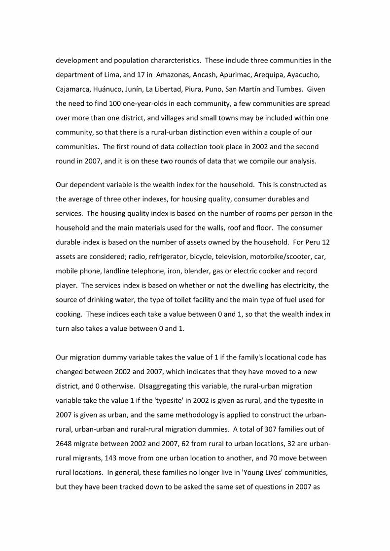
development and population chararcteristics.  These include three communities in the 

department of Lima, and 17 in  Amazonas, Ancash, Apurimac, Arequipa, Ayacucho, 

Cajamarca, Huánuco, Junín, La Libertad, Piura, Puno, San Martín and Tumbes.  Given 

the need to find 100 one‐year‐olds in each community, a few communities are spread 

over more than one district, and villages and small towns may be included within one 

community, so that there is a rural‐urban distinction even within a couple of our 

communities.  The first round of data collection took place in 2002 and the second 

round in 2007, and it is on these two rounds of data that we compile our analysis. 

Our dependent variable is the wealth index for the household.  This is constructed as 

the average of three other indexes, for housing quality, consumer durables and 

services.  The housing quality index is based on the number of rooms per person in the 

household and the main materials used for the walls, roof and floor.  The consumer 

durable index is based on the number of assets owned by the household.  For Peru 12 

assets are considered; radio, refrigerator, bicycle, television, motorbike/scooter, car, 

mobile phone, landline telephone, iron, blender, gas or electric cooker and record 

player.  The services index is based on whether or not the dwelling has electricity, the 

source of drinking water, the type of toilet facility and the main type of fuel used for 

cooking.  These indices each take a value between 0 and 1, so that the wealth index in 

turn also takes a value between 0 and 1. 

 

Our migration dummy variable takes the value of 1 if the family's locational code has 

changed between 2002 and 2007, which indicates that they have moved to a new 

district, and 0 otherwise.  DIsaggregating this variable, the rural‐urban migration 

variable take the value 1 if the 'typesite' in 2002 is given as rural, and the typesite in 

2007 is given as urban, and the same methodology is applied to construct the urban‐

rural, urban‐urban and rural‐rural migration dummies.  A total of 307 families out of 

2648 migrate between 2002 and 2007, 62 from rural to urban locations, 32 are urban‐

rural migrants, 143 move from one urban location to another, and 70 move between 

rural locations.  In general, these families no longer live in 'Young Lives' communities, 

but they have been tracked down to be asked the same set of questions in 2007 as 

those remaining in a Young Lives community.  There is only a very limited number of 

families who were in the 2002 survey but not included in the 2007 survey; this could 

be for a number of reasons, one of which could be that they moved and were unable 

to be tracked down. 

 

Table 1 below summarises the average values different indicators take for urban or 

rural non‐migrants, and for our four categories of migrants: 

 Table 1: Summary statistics 

Variable 

Urban non‐migrants 

Rural non‐migrants 

Rural‐urban migrants 

Urban‐rural migration 

Urban‐urban migration 

Rural‐rural migration 

Wealth indext   0.65 (0.17)  0.33  (0.14)  0.53  (0.18)  0.38  (0.21)  0.63  (0.20)  0.31  (0.18) Wealth indext‐1  0.61 (0.19)  0.29  (0.14)  0.36  (0.18)  0.52  (0.21)  0.62  (0.19)  0.27  (0.14) Change in wealth  0.04 (0.14)  0.04  (0.11)  0.17  (0.23)  ‐0.13  (0.17)  0.005  (0.21)  0.04  (0.19) Dad educationt  10.62 (3.35)  6.83  (3.65)  8.77  (3.96)  8.53  (4.37)  11.13  (3.33)  6.18  (3.48) Mum educationt  9.69 (3.82)  4.79 (3.85)  8.02 (4.04)  8.57 (3.51)  10.07 (3.69)  4.42 (3.21) Quechuan  0  0.21  (0.41)  0  0.06 (0.25)  0  0.06  (0.23) Indigenous  0  0.003 (0.06)  0  0  0  0 Agemumt‐1  26.7 (6.4)  27.6  (7.3)  24.5  (5.7)  24.7  (5.7)  25.9  (6.1)  25.4  (7.1) Household sizet  5.25 (2.00)  6.06 (2.09)  4.74 (1.68)  4.75 (1.37)  4.79 (1.71)  5.91 (2.18) Time lived theret‐1  16.0 (10.9)  19.7  (12.6)  11.9  (9.4)  7.9  (7.7)  12.6  (10.8)  14.6  (12.9) Prev migrationt‐1  0.36 (0.48)  0.27 (0.44)  0.50 (0.50)  0.69 (0.47)  0.49 (0.50)  0.46 (0.50) Ownhouset‐1  0.61 (0.49)  0.82  (0.38)  0.55  (0.50)  0.47  (0.51)  0.47  (0.50)  0.70  (0.46) Ownhouset   0.67 (0.47)  0.84  (0.37)  0.37  (0.49)  0.59  (0.50)  0.46  (0.50)  0.67  (0.47) Ownlandt‐1  0.20 (0.40)  0.92  (0.27)  0.65  (0.48)  0.41  (0.50)  0.20  (0.40)  0.81  (0.39) manuf sectort‐1  0.25 (0.43)  0.15  (0.36)  0.23  (0.42)  0.35  (0.49)  0.23  (0.42)  0.10  (0.30) Support networkt‐1  0.88 (0.69)  0.66 (0.69)  1.03 (0.63)  0.84 (0.57)  0.97 (0.65)  0.56 (0.69) Num groupst‐1  0.27 (0.59)  0.33  (0.63)  0.18  (0.43)  0.22  (0.49)  0.27  (0.56)  0.31  (0.60) Cog social capitalt‐1  1.35 (0.65)  1.64 (0.52)  1.43 (0.69)  1.43 (0.63)  1.33 (0.70)  1.66 (0.51) Cog social capitalt  1.07 (0.67)  1.54 (0.58)  1.08 (0.61)  1.50 (0.57)  1.08 (0.64)  1.30 (0.62) Group membert  0.27 (0.44)  0.49  (0.50)  0.24  (0.43)  0.44  (0.50)  0.24  (0.43)  0.27  (0.45) Num relativest  1.80 (1.33)  1.90  (1.29)  1.37  (1.13)  1.66  (1.12)  1.32  (1.22)  1.40  (1.26) Safe for childrent  0.18 (0.37)  0.38 (0.48)  0.14 (0.33)  0.30 (0.46)  0.15 (0.36)  0.34 (0.48) Where on laddert  5.04 (1.74)  4.74 (2.13)  4.79 (1.82)  4.34 (1.91)  5.07 (1.72)  4.36 (1.96) Expected laddert  6.88 (1.76)  6.16 (2.11)  6.39 (2.00)  6.53 (1.78)  6.99 (1.71)  6.04 (1.94) Oremitt  0.24 (0.43)  0.21  (0.40)  0.32  (0.47)  0.16  (0.37)  0.26  (0.44)  0.19  (0.39) Food shortaget  0.20 (0.40)  0.27  (0.44)  0.12  (0.32)  0.46  (0.51)  0.23  (0.42)  0.31  (0.47) Access  house assistt  0.56 (0.50)  0.16  (0.36)  0.55  (0.50)  0.41  (0.50)  0.62  (0.49)  0.14  (0.35) 

Mean values, standard deviations in parentheses.  Variables with a 'D' at the start are change variables, taking the difference between the two rounds, the subscript t‐1 denotes 2002 observations, the subscript t denotes 2007 observations.  

 Initial descriptives Columns 1 and 2  in Table 1 above  shows a  clear distinction between  those  living  in 

urban areas and those in rural communities.  The average wealth index is significantly 

higher for urban residents  in both 2002 and 2007, although the variation  in wealth  is 

also slightly higher.    Interestingly, the change  in wealth  is very similar across the two 

categories.  Parents in urban areas are likely to be more educated and have Spanish as 

their mother  tongue,  and  the  family  is more  likely  to  have moved  in  the  ten  years 

before 2002.   Social capital  indicators tend to be  lower  in urban areas, but access to 

housing assistance  is  far higher, and the  family's perception of how well off they are 

compared to others ('where on laddert') is also higher.   

 

Rural‐urban  migrants  have  an  average  initial  wealth  slightly  higher  than  the  rural 

average, and their wealth increases significantly by 2007, though it remains below the 

urban  non‐migrant  average.    Urban‐rural  migrants  had  a  wealth  index  in  2002 

comparable to that of rural‐urban migrants in 2007, and 69% of them had migrated to 

the urban community during the 10 years before 2002.  However, their average wealth 

falls significantly by 2007,  to close  to  that of rural‐urban migrants  in 2002,  though  is 

still not quite as low as the rural non‐migrant average.  Urban‐urban migrants' wealth 

remains  fairly  static,  compared  to  the  4%  increase  in  urban  non‐migrants' wealth.  

Rural‐rural  migrants  meanwhile  have  the  lowest  level  of  wealth  amongst  all  six 

categories, and their increase in wealth is comparable to that of non‐migrants. 

 

Rural‐urban migrant parents  are better educated  than  the  rural  average  and  are  all 

Spanish speakers.  Migrant mothers in general are slightly younger than non‐migrants, 

and are more mobile in terms of not being tied by home or land ownership.  Migrants 

also have  lower average cognitive social capital  in 2002, which declines  further after 

migration,  except  for  urban‐rural  migrants,  for  whom  it  increases.    Urban‐rural 

migrants  are  also  likely  to  have more  relatives  living  in  their  2007  community  than 

other migrants, suggesting  that  they are return migrants.   These urban‐rural migrant 

families perceive themselves to be worse off in 2007 than any other group (the 'where 

on  laddert'  variable), despite  their wealth  index being higher  than  the average  rural 

resident  in our sample.   However, the average urban‐rural migrant  family have quite 

high expectations for the future; they expect to be significantly better off in four years 

time, as shown by the  'expected  laddert' variable.   Urban‐urban migrants also expect 

to  be  better  off  in  the  future,  with  higher  average  expectations  than  urban  non‐

migrants.   

 

Rural‐urban and urban‐urban migrants have quite high access  to housing assistance, 

which could ease the cost of moving.  Rural‐urban migrants are the most likely to remit 

some  of  their  income,  possibly  either  to  support  rural  family members  or  to  repay 

informal loans used to fund the move. 

 

ECONOMETRIC ANALYSIS 

Initial OLS Methodology 

Our starting point is to run a reduced form regression of the level of the wealth index 

in  2007  on  a  dummy  variable  for whether  the  family  resides  in  an  urban  or  rural 

location  in 2007.   We  find a  statistically  significant coefficient on  the urban dummy, 

suggesting that, without controlling  for other  factors, urban residents enjoy a wealth 

index  31%  higher  than  that  of  rural  households.   We  then  control  for  household 

characteristics  such  as  the parents' education,  age  and ethnic background,  and  find 

that  the urban effect  falls  to 16.6%, and  is reduced  to 16.4%  if community dummies 

are also included. However, this effect is still economically and statistically significant, 

and  the  statistical  significance  of  all  but  one  of  the  community  dummies  further 

demonstrates the importance of location in determining wealth. 

 

Given that location appears to be a highly important determinant of family wealth, we 

then wish to test how changing  location affects the subsequent  level of wealth.   We 

therefore  introduce  a migration  dummy,  taking  the  value  1  if  the  family moved  (at 

least  across  a  district  boundary)  between  2002  and  2007,  and  run  a  reduced  form 

regression of 2007 wealth on this dummy variable.    In addition, we construct a more 

complete static OLS model, regressing the household's 2007 wealth index (wit) on the 

migration dummy variable (Mit) and a vector of static explanatory variables (Xit), which 

economic  theory  suggests  affect wealth  and  therefore  need  to  be  controlled  for  to 

achieve an estimate of the partial effect of migration: 

wit = δ + β Mit + γXit + uit 

 

Our results, set out in Table 2 below, show no significant effect of overall migration on 

the subsequent wealth index, either with or without the inclusion of control variables.  

 

However, we  then  separate migration  into  four different dummy  variables;  rural‐to‐

urban migration (RUit), urban‐to‐rural migration (URit), urban‐to‐urban migration (UUit) 

and rural‐to‐rural migration (RRit): 

wit = δ + β1 RUit + β2 URit + β3 UUit + β4 RRit + γXit + uit 

 

This  distinction  changes  our  results  dramatically.   Once we  control  for whether  the 

family lived in a rural or urban location in 2002, we observe statistically sIgnificant and 

opposite  effects  for  rural‐urban  migration  as  opposed  to  urban‐rural  migration.  

Including household characteristics in our set of explanatory variables (Xit), reduces the 

coefficients  on  rural‐urban  and  urban‐rural  migration  somewhat,  but  they  remain 

substantial and significant at any significance level.  The negative coefficient on urban‐

urban migration also becomes significant at  the 2%  level,  though  the effect of  rural‐

rural migration remains insignificant.   

 

However,  this  static  model  does  not  account  for  what  we  expect  to  be  a  fairly 

persistent nature of wealth, such that, even for migrants, the  level of wealth  in 2007 

will still be quite strongly related to the level of wealth in 2002.  We therefore extend 

our static model to a dynamic model, which includes the wealth index in 2002 (wit‐1): 

wit = δ + β Mit + ф wit‐1 + γXit + uit      and 

wit = δ + β1 RUit + β2 URit + β3 UUit + β4 RRit + ф wit‐1 + γXit + uit 

 

We  find  that wit‐1 does  indeed have  a  strong  effect on wit,  increasing  the extent  to 

which our explanatory variables explain the 2007 level of wealth, as demonstrated by 

the rise  in the R‐squared value.   However, adding this dynamic element to the model 

also  introduces  the endogeniety problem of wit‐1 being  correlated with uit.   We also 

have reason to believe that 2002 wealth may be correlated with our migration dummy 

variables, since  theory suggests  that a certain  initial  level of wealth  is a  requirement 

for migration,  given  the  relocation  costs.    In  addition,  higher  initial wealth may  be 

correlated with migration via other  factors  such as education and  skills; more highly 

skilled workers are likely to earn more in 2002, and are also more likely to migrate to a 

more urban  location.   Therefore,  the endogeneity of  the  lagged dependent  variable 

could bias our results.   

 

However, our  regression  coefficients on  the migration variables differ  little between 

the static and dynamic models; only the coefficient on urban‐rural migration is slightly 

reduced.  Overall, our OLS results suggest that rural‐urban migration is associated with 

an  average  14%  increase  in  the  subsequent wealth  index,  urban‐rural migration  is 

associated with  an  average 21‐24% decrease  in household wealth,  and urban‐urban 

migration is linked to an average 4% reduction in 2007 wealth. 

Table 2: OLS results for the level of wealth 

 Urban effect 

Location effect + controls  Migration 

+ static controls 

Type  of migration 

control for urbant‐1 

+ static controls 

+ dynamic control 

VARIABLES  Wit  Wit  Wit  Wit  Wit  Wit  Wit  Wit Urbant  0.313***  0.164***             Migration      ‐0.0098  ‐0.0094         RU          0.0087  0.194***  0.138***  0.138*** UR          ‐0.141***  ‐0.276***  ‐0.239***  ‐0.209*** UU          0.109***  ‐0.0262  ‐0.0389**  ‐0.0353** RR          ‐0.208***  ‐0.0231  0.0229  0.0146 Urbant‐1        0.141***    0.320***  0.170***  0.106*** Daded    0.0102***    0.0110***      0.0105***  0.0055*** Mumed    0.0131***    0.0137***      0.0131***  0.0078*** Quechua    ‐0.0268**    ‐0.041***      ‐0.029**  ‐0.030*** Indigen    ‐0.238***    ‐0.246***      ‐0.236***  ‐0.179*** Hhsize    0.0032*    0.0023      0.0026  0.0034** Agemum    ‐0.0316*    ‐0.0326*      ‐0.0325**  ‐0.0286* Agemumsq    0.0011**    0.0012**      0.0012**  0.0010** Agemumcub    ‐0.000**    ‐0.000**      ‐0.000**  ‐0.000* Housingasist    0.037***    0.0478***      0.0407***  0.0341*** Foreignremit    0.080***    0.081***      0.078***  0.064*** Wit‐1                0.408*** Lima01    0.191***    0.186***      0.183***  0.083*** Lima02    0.173***    0.169***      0.166***  0.0638** Lima03    0.198***    0.197***      0.193***  0.090*** Community4    0.168***    0.155***      0.166***  0.069*** Community5    0.116***    0.113***      0.110***  0.043* Community6    0.109***    0.107***      0.105***  0.022 Community7    0.146***    0.145***      0.136***  0.072*** Community8    0.136***    0.130***      0.126***  0.064** Community9    0.0842***    0.0778***      0.0807***  0.020 Community10    0.124***    0.122***      0.120***  0.064** Community11    ‐0.008    ‐0.008      ‐0.017  ‐0.015 Community12    0.105***    0.100***      0.105***  0.041** Community13    0.206***    0.209***      0.207***  0.113*** Community14    0.111***    0.109***      0.109***  0.059*** Community15    0.054***    0.051***      0.052***  0.025 Community16    0.092***    0.104***      0.091***  0.030 Community17    0.139***    0.143***      0.137***  0.076*** Community18    0.052**    0.061***      0.059***  0.019 Community19    0.094***    0.098***      0.095***  0.044** Constant  0.330***  0.327**  0.517***  0.347**  0.517***  0.331***  0.342**  0.323**                  Observations  2647  1886  2647  1886  2647  2647  1886  1882 R‐squared  0.472  0.656  0  0.635  0.04  0.479  0.659  0.715 

Robust standard errors in parentheses    *** p<0.01, ** p<0.05, * p<0.1  

 However,  there may  be  other  factors  that  we  have  not  controlled  for  in  our  OLS 

regression, that influence  both the decision to migrate and the level of wealth in 2007.  

According  to  the  R‐squared  value,  our  regression  only  explains  up  to72%  of  the 

variation  in the 2007 wealth  index across households.   Therefore, there  is substantial 

potential for omitted variables to be important in determining wealth, and these could 

potentially be correlated with migration, biasing our point estimates.   Such variables 

could include unobservable household characteristics, such as the ability of the wage‐

earners in the household.  If these characteristics change the future expected income 

of the family, they are also likely to be correlated with a decision on whether or not to 

migrate,  since  this  is  itself,  according  to  our  theories,  based  to  a  large  extent  on 

expected wages. 

 

Difference‐in‐Differences Methodology 

Taking first differences to consider change variables, such as the change in wealth,  can 

eliminate  the  self‐selection  bias  caused  by  the  unobservable,  time‐invariant 

characteristics that drive both migration and the subsequent level of wealth.   

The difference‐in‐differences estimator compares the difference in average household 

wealth before and after migration for migrating households, with the before and after 

contrast for non‐migrating households,  i.e. how a change  in  location could result  in a 

change in wealth.   

∆wit  = δ + β Mit + γ ∆Xit + uit  and  ∆wit   = δ + β1 RUit + β2 URit + β3 UUit + β4 RRit + γ 

∆Xit + uit 

where ∆Xit  is a vector of change variables that could directly  influence the change  in 

wealth. 

 

We  can  therefore  interpret  the  results  below  as  fixed  effects  results,  for  our  two‐

period panel.  Overall migration again does not appear to affect the change in wealth, 

with or without control variables.  However, separating migration by type continues to 

give strong results.  The coefficient on rural‐urban migration has fallen slightly, to 13% 

(with or without the  inclusion of change variables as controls), and the coefficient on 

urban‐rural migration has been reduced more substantially, to 16%, once controls are 

included.   

 

Table3: Difference‐in‐differences results 

  Migration + change controls 

Type migration 

+ change controls 

+ level effects 

robustness check 

VARIABLES  Dwi  Dwi  dwi  Dwi  Dwi  Dwi Migration  ‐0.0090  ‐0.0039         RU      0.126***  0.129***  0.146***  0.0945*** UR      ‐0.176***  ‐0.158***  ‐0.155***  ‐0.153*** UU      ‐0.0364**  ‐0.0319*  ‐0.0335  ‐0.016 RR      0.0032  0.0049  0.0088  ‐0.0197 Dhhsize    0.0067***    0.0063***  0.0060***  0.0047*** Downhouse    ‐0.007    ‐0.0036  ‐0.0010  ‐0.0051 Newbirth    ‐0.0317***    ‐0.0275***  ‐0.0342***  ‐0.0354*** Employershut    ‐0.0096    ‐0.0071  ‐0.0198  ‐0.0063 lostincomesource    ‐0.0013    ‐0.0035  ‐0.0054  ‐0.0019 Landdispute    ‐0.110**    ‐0.0960**  ‐0.0867  ‐0.0674 assetdispute    0.114***    0.1139***  0.126***  0.118*** Cropfail    0.0379**    0.0361**  0.0483**  0.0104 pestdisease    ‐0.0342    ‐0.0325  ‐0.0310  ‐0.0500 Daddied    ‐0.0586    ‐0.0410  ‐0.0723  ‐0.0664 Divorce    ‐0.0161    ‐0.0179  ‐0.0154  0.0021 Davclustwi    1.127***    1.130***  1.094***  0.413** Daded          ‐0.0014  0.0051*** Mumed          ‐0.0009  0.0076*** agemum1          ‐0.0003  0.0010** Quechua          ‐0.0170  ‐0.0273** Indigen          ‐0.0632**  ‐0.1442*** wi1            ‐0.382*** Constant  0.0409***  0.00044  0.0409***  ‐0.00031  0.0350*  0.0797*** Observations  2636  2636  2636  2636  1883  1883 R‐squared  0  0.041  0.039  0.076  0.090  0.263 

  

Robustness Checks 

As a robustness check, we include level effects of education, age and ethnic group, and 

find  that  the  coefficient  on  rural‐urban migration  increases  a  little  to  15%.    As  a 

robustness check across both our levels and changes regressions, we also try including 

initial 2002 wealth as a variable  influencing the subsequent change  in wealth.   Again, 

the  coefficient on  rural‐urban migration moves,  this  time decreasing  to 9%, but  this 

coefficient and that on urban‐rural migration remain statistically significant. 

 

These results are also robust to using only those who have considered moving as the 

non‐migrant  control  group,  i.e.  those  who  may  have  had  the  most  similar 

unobservable characteristics to the actual migrants.   They are also robust to using an 

alternative,  propensity  score matching method, with matching  based  on  our  probit 

model for the decision to migrate, set out in the Annex.  The average treatment effect 

of rural‐urban migration on the migrants is a statistically significant 16‐20% increase in 

wealth across the three matching methods10, whilst the average effect of urban‐rural 

migration is a statistically significant 19‐23% decline in wealth.  The average treatment 

effect on urban‐urban migrants was  low, negative and  insigificant, and that on rural‐

rural migrants was very low, positive and highly insignificant.    

 

Our  findings are also  robust  to breaking  the wealth  index down and considering  the 

effect of the different types of migration on each of the three components of wealth; 

housing  quality,  consumer  durables  and  services.    The  coefficient  on  rural‐urban 

migration  remains  positive  and  the  coefficient  on  urban‐rural  migration  remains 

negative across all three indexes.  The coefficient for urban‐urban remains negative for 

housing  quality  and  services,  but  turns  positive,  though  insignificant,  for  consumer 

durables. 

 Therefore, across all these models, though our point estimates change somewhat, our 

results  persistently  show  that  rural‐urban  migration  is  linked  to  a  substantial 

improvement in household wealth and living standards, whilst urban‐rural migration is 

associated with an even more substantial reduction  in the family's standard of  living.  

This  does  not mean  that  the wealth  index  increases  for  every  rural‐urban migrant 

family and decreases for every urban‐rural family; the change in wealth ranges from ‐

0.36  to  +0.69  for  rural‐urban  migrants,  and  from  ‐0.42  to  +0.12  for  urban‐rural 

migrants.  However, for the most part, rural‐urban migrants do enjoy an improvement 

in their standard of living, as proxied by the wealth index, whilst urban‐rural migrants 

see their living conditions deteriorate.  

 

Instrumental Variable Estimation 

The  difference‐in  diffences method  controlled  for  time‐invariant  omitted  variables, 

such as household risk aversion and ability.   We have also controlled for a number of 

10 The three propensity score matching methods used are Kernel Matching, Nearest Neighbour Matching and the Stratification Method.  

observed  time‐variant  variables,  such  as  a  loss  of  income  source,  the  place  of 

employment being shut down or destroyed, the birth of a new child, the death of the 

main  income  earner,  crop  failure,  etc.    However,  we  are  highly  unlikely  to  have 

captured all the factors changing the household's wealth during the 2002‐2007 period.  

There are other unobserved time‐variant variables that we cannot proxy for, but which 

could drive both  the decision  to migrate  and  the  change  in wealth.    These omitted 

variables,  if they are correlated with both the migration variable and the error term, 

create  an  endogeneity  bias  in  our  estimates  of  the  effect  of  migration.    If  these 

unobserved changes  increase both  the  likelihood of migration and  the change  in  the 

wealth  index,  then  our  estimate  of  the  effect  of migration  is  likely  to  be  upwardly 

biased.    However,  our  estimate  could  also  be  biased  downwards,  if  unobservable 

negative events both cause  the  family  to  leave  their original community and  reduce 

wealth.   This  is  linked to our other concern, that of reverse causality.    It may well be 

that  a  change  in wealth  during  the  period,  for whatever  reason,  drives,  enables  or 

forces  subsequent migration.   Again,  this  reverse  causality  could  cause  us  to  either 

overestimate  the benefits of migration,  if an  increase  in wealth means  that a  family 

can afford to migrate, or overestimate the costs of migration,  if a decrease  in wealth 

drives the family to search for opportunities elsewhere.   

 

This  latter  form  of  reverse  causality  in  particular  could  be  biasing  our  urban‐rural 

migration results; if unobserved urban unemployment or underemployment decreases 

wealth to the point where the family cannot afford the cost of urban living, they may 

be  forced  to  leave  the  city.    There may  be  further  losses  in wealth  and  access  to 

services as a  result of  the move, but we cannot  infer  from our coefficient on urban‐

rural migration  that  this migration causes  the  full 16% decrease  in  the wealth  index; 

we expect that the effect of the move itself is substantially lower, and if we continue to 

view migration as a rational investment choice, the urban‐rural migrant family may be 

choosing  to move  away  from what  they  expected  could  have  been  an  even worse 

decline  in wealth  if  they  had  remained  in  the  city,  at  least  in  the  long‐run,  i.e.  net 

present value expected returns to migration outweigh the short‐run costs of the move.  

We have  controlled  for unemployment  and  loss of  income  as  far  as possible  in our 

change variables, but unobserved underemployment  in particular  is  likely to still be a 

cause of endogeneity. 

 

We therefore believe that Mit and uit may well be correlated: Cov(Mit,uit) ≠ 0, and so 

we use the method of instrumental variables (two‐stage least squares) to address this 

endogeneity. 

 

We  need  instrumental  variables  for Mit,  labelled  Zit‐1,  that  are  correlated  with,  or 

influence, the decision to migrate; Cov(Zit‐1,Mit) ≠ 0, but that do not effect the change 

in wealth other  than  through migration; Cov(Zit‐1,uit) = 0. We  therefore  consider  the 

theoretical  push  and  pull  factors  believed  to  drive  migration  (as  discussed  in  the 

Annex), and estimate a probit model for the probability of migrating: 

Mit = δ + β Xit + θ Zit‐1 + v 

 

where Xit  is a vector of variables  that we believe affect  the decision  to migrate, but 

which may also directly affect  the change  in wealth, and Zit‐1  is a vector of variables 

influencing migration, which are measured at the start of the period, and which we do 

not believe would change wealth during the period, other than through migration. The 

results of the probit regression are set out in the Annex.   

 

This  regression gives us  two potential  instrumental variables, which had a significant 

effect on the probability of migrating, and which we believe are exogenous.  These are 

'support networks', indicating whether family and friends provided help and support in 

2002, and  'previous migration', a dummy  variable  for migration during  the 10  years 

preceeding 2002.  We use support networks as a proxy for the migration opportunities 

available  to  rural  inhabitants;  family  and  friends  are  assumed  to  provide  both  help 

finding urban work and help funding the  investment  in migration.    If we run a probit 

regression  just  for  rural‐urban migration we  find  that  the  support  network  variable 

becomes more  important, with a coefficient of 0.31, significant at the 1% significance 

level.   

 

If we run a probit regression  just  for urban‐rural migration, we  find that the support 

network  effect  becomes  statistically  insignificant,  but  the  coefficient  on  previous 

migration  rises  to  0.54,  significant  at  the 1%  level.   Our  theory  suggests  that urban 

migrant families may be  invovled  in return or step migration.   With  less roots  in their 

current urban community, and former or continued connections elsewhere, those who 

immigrated  in  the  recent past are more  likely  to move again.   However, we assume 

that migration has an effect on the change in wealth upon or soon after migration, and 

that migration  in the ten years before 2002 should not change wealth between 2002 

and 2007, other than through repeat migration.   

 

Given that both support networks and previous migration are observed  in 2002, they 

cannot be driven by the change in wealth between 2002 and 2007, so these variables 

should not be endogenous due  to  reverse  causality.   Whilst  these  variables may be 

correlated with  the  level of wealth, we do not believe  that  they cause a subsequent 

change in wealth, other than through migration (although we will return to this point 

later).  We therefore use support networks as an instrumental variable for rural‐urban 

migration, and previous migration as an  instrument  for urban‐rural and urban‐urban 

migration, with the results given in Table 4 below. 

 

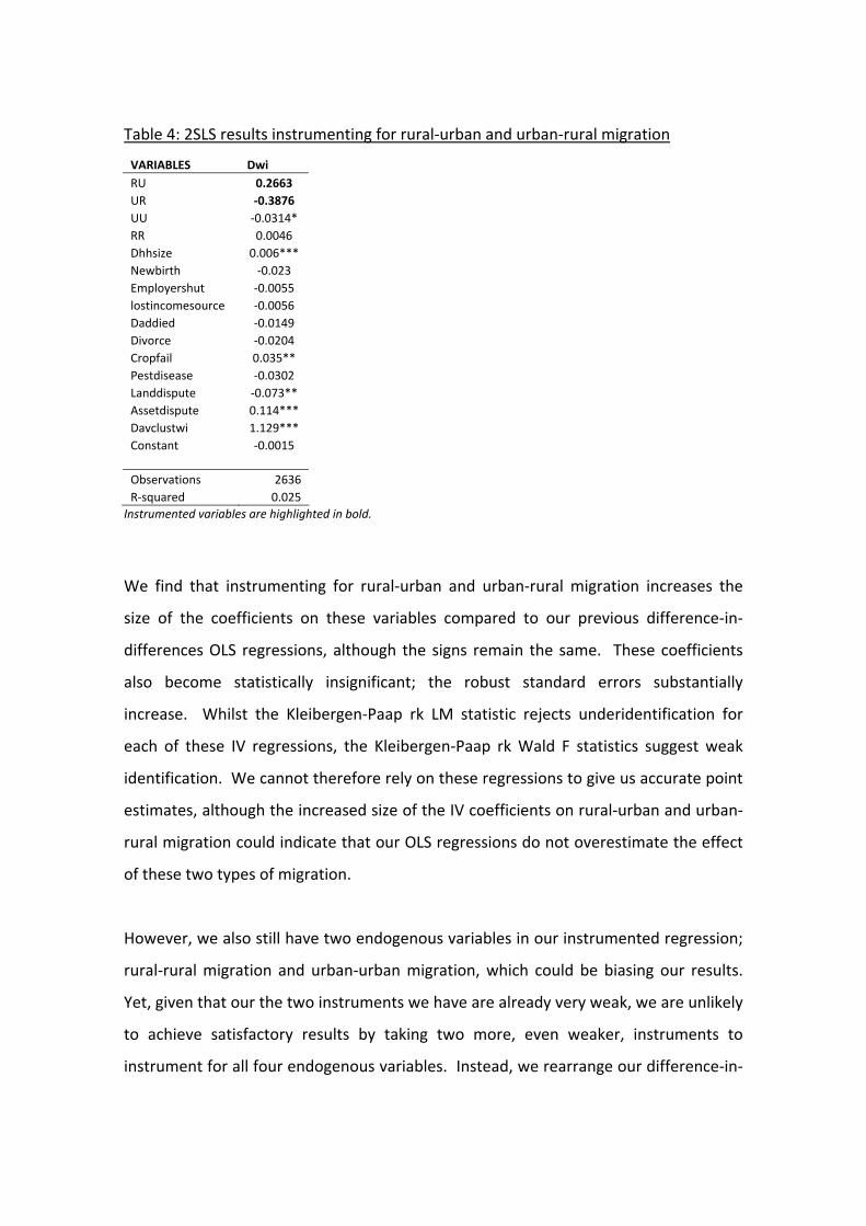
Table 4: 2SLS results instrumenting for rural‐urban and urban‐rural migration 

VARIABLES  Dwi RU  0.2663 UR  ‐0.3876 UU  ‐0.0314* RR  0.0046 Dhhsize  0.006*** Newbirth  ‐0.023 Employershut  ‐0.0055 lostincomesource  ‐0.0056 Daddied  ‐0.0149 Divorce  ‐0.0204 Cropfail  0.035** Pestdisease  ‐0.0302 Landdispute  ‐0.073** Assetdispute  0.114*** Davclustwi  1.129*** Constant  ‐0.0015    Observations  2636 R‐squared  0.025 

Instrumented variables are highlighted in bold. 

  

We  find  that  instrumenting  for  rural‐urban  and  urban‐rural migration  increases  the 

size  of  the  coefficients  on  these  variables  compared  to  our  previous  difference‐in‐

differences OLS  regressions, although  the signs  remain  the same.   These coefficients 

also  become  statistically  insignificant;  the  robust  standard  errors  substantially 

increase.   Whilst  the  Kleibergen‐Paap  rk  LM  statistic  rejects  underidentification  for 

each of  these  IV  regressions,  the Kleibergen‐Paap  rk Wald  F  statistics  suggest weak 

identification.  We cannot therefore rely on these regressions to give us accurate point 

estimates, although the increased size of the IV coefficients on rural‐urban and urban‐

rural migration could indicate that our OLS regressions do not overestimate the effect 

of these two types of migration.   

 

However, we also still have two endogenous variables in our instrumented regression; 

rural‐rural migration and urban‐urban migration, which  could be biasing our  results.  

Yet, given that our the two instruments we have are already very weak, we are unlikely 

to  achieve  satisfactory  results  by  taking  two  more,  even  weaker,  instruments  to 

instrument for all four endogenous variables.  Instead, we rearrange our difference‐in‐

differences equation  in  terms of  two endogenous  variables;  the decision  to migrate 

(Mit) and whether the family ends up in an urban or rural location (urbanit, shortened 

to Uit).  Whether the initial location is urban or rural (Uit‐1) is taken as exogenous: 

∆wit = δ + β1 Uit Mit+ β2 Uit‐1 Mit+ β3 Uit‐1 Uit Mit+ β4 Mit + γ ∆Xit + uit 

 

Which,  given  our  negligible  coefficient  on  overall  migration,  we  can  write  more 

eloquently as two interaction terms: 

∆wit = δ + β4 Mit .( 1 + β5 Uit ).( 1 + β6 Uit‐1 ) + γ ∆Xit + uit 

where  β5 = β1/β4,     β6= β2/β4,   and   β3 = β4β5β6 

 

We now run a probit regression for each of our two endogenous variables; one for the 

probability of ending up in an urban location, and one for the probability of deciding to 

migrate  (our  probit  regression  from  before).    Both  of  these  include  our  two 

instrumental variables, and are set out in the Annex. 

 

We  then  take  the predicted values  from each of  these  first stage probits and run an 

intermediate second stage OLS regression for urbanit on  its own predicted value, and 

for Mit on its own predicted value.  The residuals from these intermediate regressions 

(ehatit and mhatit respectively) are then  included  in our final second stage regression, 

the results of which are set out in Table 6 below: 

 

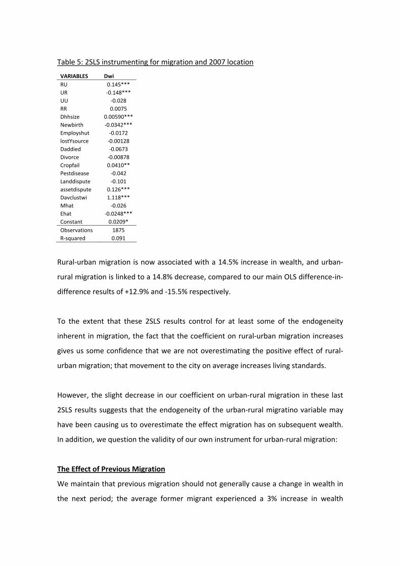
Table 5: 2SLS instrumenting for migration and 2007 location 

VARIABLES  Dwi RU  0.145*** UR  ‐0.148*** UU  ‐0.028 RR  0.0075 Dhhsize  0.00590*** Newbirth  ‐0.0342*** Employshut  ‐0.0172 lostYsource  ‐0.00128 Daddied  ‐0.0673 Divorce  ‐0.00878 Cropfail  0.0410** Pestdisease  ‐0.042 Landdispute  ‐0.101 assetdispute  0.126*** Davclustwi  1.118*** Mhat  ‐0.026 Ehat  ‐0.0248*** Constant  0.0209* Observations  1875 R‐squared  0.091 

 

Rural‐urban migration  is now associated with a 14.5%  increase  in wealth, and urban‐

rural migration is linked to a 14.8% decrease, compared to our main OLS difference‐in‐

difference results of +12.9% and ‐15.5% respectively. 

 

To  the  extent  that  these  2SLS  results  control  for  at  least  some  of  the  endogeneity 

inherent  in migration, the fact that the coefficient on rural‐urban migration  increases 

gives us some confidence that we are not overestimating the positive effect of rural‐

urban migration; that movement to the city on average increases living standards. 

 

However, the slight decrease  in our coefficient on urban‐rural migration  in these  last 

2SLS results suggests that the endogeneity of the urban‐rural migratino variable may 

have been causing us to overestimate the effect migration has on subsequent wealth.  

In addition, we question the validity of our own instrument for urban‐rural migration:   

 

The Effect of Previous Migration 

We maintain that previous migration should not generally cause a change in wealth in 

the  next  period;  the  average  former migrant  experienced  a  3%  increase  in wealth 

between 2002‐2007, and only 3 of the 579 former urban migrants were not involved in 

any  recorded activity  in 2002.   This  supports de Brauw and Giles'  (2006)  suggestion 

that migrants look to establish employment in the city before the family relocates, so 

unemployment  on  arrival may  be  low,  possibly  even  lower  than  the  Harris‐Todaro 

model might predict.   

 

However, there  is a case for arguing that some former migrants are more susceptible 

to becoming unemployed at a  later stage than theirnon‐migrant counterparts.   Some 

migrants may only be employed on temporary contracts, and may be the first to  lose 

their jobs if unemployment rises, as it did in Peru between 2001 and 2005, from below 

8%  to nearly 10%.   Underemployment was also estimated  to have begun  increasing 

again in 1997‐2002, to over half the country's population11. 

 

Unskilled migrants often work in the informal services sector, some running their own 

small businesses, and are particularly vulnerable to a loss of business if demand 

declines.  As the Harris‐Todaro theory noted, they often join this sector because of the 

ease of entry, but by the same token there is also little job security.  For example, this 

year in China, it is estimated that there are 20 million and rising unemployed urban 

migrants, many of whom are expected to return to rural areas, and during the Asian 

crisis, Thailand experienced a disproportionate amount of urban‐rural return 

migration, compared to the average rise in unemployment for the total population.   

 

If  former migrants are more  susceptible  to adverse  shocks  in  this way, our previous 

migration  variable  will  be  correlated  with  the  error  term  in  our  change  in  wealth 

regression, and  is no  longer a valid  instrument.   Since  the variables  in our  first stage 

probit  regression are correlated with migration,  they are also  likely  to be correlated 

with previous migration, and therefore we would no longer have a valid instrument.   

 

11 http://siteresources.worldbank.org/INTPROSPECTS/Resources/334934-1199807908806/Peru.pdf

Further Analysis 

Therefore,  the possibility of  reverse  causality; a  shock  causing a decrease  in wealth, 

which in turn leads to urban‐rural migration, remains our primary concern.  We believe 

that  this  reverse  causality may  be  biasing  our  estimate  of  the  cost  of  urban‐rural 

migration upwards.   However, we also maintain that, even  if we could eliminate this 

endogeneity,  urban‐rural migrants  could  still  be materially worse  off  than  the  true 

counterfactual in the short run, due to relocation costs; i.e. some of the causality is still 

running from urban‐rural migration to the observed change in wealth. 

 

We return to the difference‐in‐differences approach and look at each type of migration 

in more  detail,  breaking  them  down  by  the  reason  the  family  gave  for  why  they 

migrated12, and also looking at the distance the family moved. 

12 Note that only two‐thirds of migrant households gave a response to this question. 

 Table 6: Why migrants move, and the distance moved 

Why  Dwi      Distance  dwi   

RUwork  0.194***      RUdistrict  0.164***   

RUinvest  0.127      RUprovince  0.136**   

RUperson  0.127**      RUdepartmt  0.102**   

URwork  ‐0.156***      URdistrict  ‐0.0847**   

URinvest  ‐0.0741***      URprovince  ‐0.196***   

URperson  ‐0.0893**      URdepartmt  ‐0.161***   

UUwork  ‐0.00968      UUdistrict  ‐0.0207   

UUinvest  0.0872*      UUprovince  ‐0.0685   

UUperson  ‐0.0614*      UUdepartmt  ‐0.0291   

RRwork  ‐0.0105      RRdistrict  0.00384   

RRinvest  0.0609      RRprovince  0.0324   

RRperson  ‐0.0346      RRdepartmt  ‐0.00673   

Dhhsize  0.00622***      Dhhsize  0.00627***   

Newbirth  ‐0.0269***      Newbirth  ‐0.0285***   

Employershut  ‐0.00701      Employershut  ‐0.00821   

Lostincomesource  ‐0.00842      Lostincomesource  ‐0.00602   

Landdispute  ‐0.0957**      Landdispute  ‐0.0935**   

Assetdispute  0.114***      Assetdispute  0.113***   

Cropfail  0.0387**      Cropfail  0.0367**   

Pestdisease  ‐0.0316      Pestdisease  ‐0.0317   

Daddied  ‐0.0624      Daddied  ‐0.0361   

Divorce  ‐0.0167      Divorce  ‐0.0178   

Davclustwi  1.139***      Davclustwi  1.123***   

Constant  ‐0.00207      Constant  ‐2.36E‐05   

Observations  2636      Observations  2636   

R‐squared  0.07      R‐squared  0.079   

  

Disagrregating the types of migration by the reason the family give for moving shows 

that  the coefficient on  rural‐urban migration  remains positive and  the coefficient on 

urban‐rural migration remains negative across the three groups of reasons for moving; 

for work, for investment (in health or education) and for personal reasons.  Migrating 

from rural to urban areas for work gives the highest coefficient, suggesting that these 

migrants benefit from higher urban wages, but migrating to the city for other reasons 

is also correlated with an substantial increase in the wealth index, which could reflect 

either  a  change  in wealth  that enables  them  to migrate  for  investment or personal 

reasons, or an improvement in living standards as a result of the move, or as a result of 

the investment the family moved to achieve. 

 

The negative coefficient on urban‐rural migration for work  is twice as high as that on 

urban‐rural migration for investment or personal reasons.  This supports the possibility 

of  reverse  causality, whereby  a  reduction  in  earnings  forces  the migrant  family  to 

move out of the city in search of work, and therefore a decrease in wealth has caused 

migration.  However, the loss of wealth associated with urban‐rural migration for other 

reasons  is  still  around  7‐9%  and  significant,  which  could  indicate  that  choosing  to 

migrate out of urban areas could also be associated with a reduction in wealth, at least 

over the short‐term, but not as much as our coefficients on urban‐rural migration as a 

whole  implied.   These families may still view migration as an  investment  if they value 

the reasons they give for moving more highly than the material goods we  included  in 

our wealth  index.   For example, social  indicators; group membership, cognitive social 

capital, safety for children, are shown  in Table 1 to be generally higher  in rural areas 

than in cities, and these aspects of non‐material well‐being may be of greater value to 

the family than material assets. 

 

Disaggregating  the  types of migration by distance  shows  the benefits of  rural‐urban 

migration to be highest when migration occurs within a province, and then declining 

with distance.   The cost of urban‐rural migration  is also only half as high  for within‐

province migration compared  to migration across provincial borders.    If distance  is a 

proxy for one‐off relocation costs (Falaris, 1979), these results suggest that these one‐

off  costs  could  be  significant,  supporting  the  suggestion  that  it  is migration  that  is 

causing  at  least  some  of  the  short‐term  loss  in wealth  experienced  by  urban‐rural 

migrants,  but  that  they  are willing  to  forego  this  short‐term wealth  due  to  other, 

longer‐term motivations for migration.   

 

CONCLUDING REMARKS 

Our  findings  suggest  that  on  average,  rural‐to‐urban  migrants  experience  an 

improvement  in  their material  standard  of  living,  consistent with  the Harris‐Todaro 

model,  but  that  the  opposite  is  the  case  for  urban‐rural migrants,  and  to  a  lesser 

extent for urban‐to‐urban migrants.    

 

This  may  be  to  some  extent  because  we  have  inadequately  controlled  for  the 

endogeneity of  the mgiration  variable, and  it  is  the  change  in wealth  that  is driving 

migration out of the city; if migration is a rational choice, then the outcome associated 

with  remaining  in  the  city  was  expected  to  be  either  even  worse  than  the  post‐

migration outcome we observe, or  it was expected to be worse than the reutrn from 

migration in the longer term.   

 

However, there is also reason to believe that we could observe these results even with 

an exogenous migration variable.  It could be that urban‐rural migration does cause a 

decline  in  wealth,  but  that  the  urban‐rural  migration  decision  is  driven  by  other 

factors, which  take  precedence  over material  living  standards  as measured  by  our 

wealth  index.   Or,  if we  return  to  the  theoretical  view of migrants being by nature 

entrepreneurs  willing  to  risk  short‐run  relocation  costs  and  the  possibility  of 

unemployment  for  long‐term  gains,  then  it  could  be  the  case  that  urban‐rural 

migration  is  a  longer‐term  form of  investment  than  rural‐urban migration,  and may 

involve a higher  loss of assets  in the short‐term, possibly  in order to  invest  in  land or 

equipment,  which  is  something  we  have  not  been  able  to  control  for  within  our 

dataset.   Certainly our  'expected  ladder' variable  in the summary statistics  in Table 1 

suggests that the average urban‐rural migrant expects to be considerably better off in 

four years time than they are in 2007.  On balance, we suggest that our findings reflect 

the presence of both of these effects; an adverse shock as a push factor for urban‐rural 

migration, and the pull of longer‐term, or non‐material‐wealth benefits. 

 

ANNEX 

The Drivers of Migration 

Todaro & Smith (2006) note that, in addition to wage differentials, age and education, 

migration  is also explained partly by  relocation upon  remarrying, prior emigration of 

family  members,  distance  and  costs  of  relocation,  occurrence  of  famine,  disease, 

violence and other disasters, and relative standing in the origin community, with those 

lower  on  the  social  order more  likely  to migrate.   Migration  can  also  be  a  form  of 

portfolio diversification of families who seek to settle some members  in areas where 

they have are likely to experience dissimilar shocks, at differing times.  Paulson (2000) 

also found that insurance motives appeared to drive migration within Thailand. 

 

Goss  &  Schoening  (1984)  find  that  migration  decreases  with  the  duration  of 

unemployment, suggesting that a reduction in assets may lower the ability to migrate.  

Lansing & Mueller  (1967)  show  that many migrants are  influenced by  such  issues as 

family  location  and health, with  family proximity  and  temperate  climate being non‐

wage advantages of any given location. 

 

Polachek & Horvath (1977) and Plane (1993) find that migration propensities do vary 

with age.  Workers are most likely to migrate during their early twenties, and then the 

propensity to move declines with age thereafter, as the time period over which to reap 

gains from migration shortens.  They also find that migration increases with education.  

The  more  highly  educated  work  in  wider  labour  markets,  and  tend  to  be  better 

informed  about  opportunties  outside  their  local  labour market,  and  better  able  to 

evaluate that information. 

 

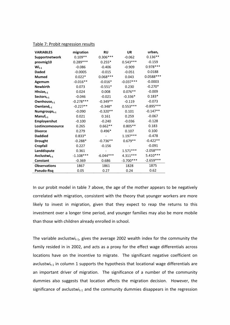
Table 7: Probit regression results 

VARIABLES  migration  RU  UR  urbant 

Supportnetwork  0.109**  0.306***  ‐0.062  0.136** prevmig10  0.289***  0.255*  0.543***  ‐0.159 Wit‐1  ‐0.086  ‐0.406  ‐0.909  0.978*** Daded  ‐0.0005  ‐0.015  ‐0.051  0.0188 Mumed  0.022*  0.068***  0.043  0.0588*** Agemum  ‐0.016**  ‐0.016*  ‐0.037***  ‐0.0003 Newbirth  0.073  ‐0.551*  0.230  ‐0.270* Hhsizet‐1  0.024  0.008  0.076**  ‐0.009 Sectorst‐1  ‐0.046  ‐0.021  ‐0.336*  0.183* Ownhouset‐1  ‐0.278***  ‐0.349**  ‐0.119  ‐0.073 Ownlandt‐1  ‐0.227**  ‐0.348*  0.553***  ‐0.895*** Numgroupst‐1  ‐0.090  ‐0.320**  0.101  ‐0.147** Manuft‐1  0.021  0.161  0.259  ‐0.067 Employershut  ‐0.100  ‐0.240  ‐0.036  ‐0.128 Lostincomesource  0.265  0.662**  0.805**  0.183 Divorce  0.279  0.496*  0.107  0.100 Daddied  0.833*  ‐  1.197***  ‐0.478 Drought  ‐0.288*  ‐0.736**  0.679**  ‐0.422** Cropfail  0.227  ‐0.156  ‐  ‐0.091 Landdispute  0.361  ‐  1.571***  ‐2.058*** Avclustwit‐1  ‐1.108***  ‐6.044***  4.311***  5.410*** Constant  ‐0.369  0.686  ‐3.700***  ‐2.659*** Observations  1867  1861  1828  1875 Pseudo‐Rsq  0.05  0.27  0.24  0.62 

  In our probit model  in table 7 above, the age of the mother appears to be negatively 

correlated with migration, consistent with the theory that younger workers are more 

likely  to  invest  in  migration,  given  that  they  expect  to  reap  the  returns  to  this 

investment over a longer time period, and younger families may also be more mobile 

than those with children already enrolled in school. 

 

The variable avclustwit‐1, gives the average 2002 wealth  index for the community the 

family resided  in  in 2002, and acts as a proxy  for the effect wage differentials across 

locations  have  on  the  incentive  to migrate.    The  significant  negative  coefficient  on 

avclustwit‐1  in column 1 supports the hypothesis that  locational wage differentials are 

an  important  driver  of migration.    The  significance  of  a  number  of  the  community 

dummies  also  suggests  that  location  affects  the migration  decision.    However,  the 

significance of avclustwit‐1 and  the community dummies disappears  in  the  regression 

for  rural‐urban migration,  which  is  surprising;  we  would  expect  higher  rural‐urban 

migration from poorer rural areas, where local opportunities were limited.  It could be 

that  the  statistical  insignificance  of  these  variables  in  the  rural‐urban  migration 

regression  is  due  to  correlations  between  our  explanatory  variables;  the  locational 

effect  is being picked up by other variables that tend to differ by  location.   However, 

even  in  a  reduced  form  probit  regression  of  rural‐urban  migration  on  avclustwit‐1 

amongst  just  the  rural  communities,  the  coefficient  on  avlcustwit‐1  remains 

insignificant.   

 

This  suggests  that  other  factors,  such  as  opportunities  for migration,  could  be  as 

important  as  wage  differentials  in  determining  rural‐urban  migration.    Support 

networks in particular appear to have a strong positive correlation with the decision to 

migrate  from  a  rural  area  to  an urban  centre,  and  the mother's education  is  also  a 

significant determinant.    Interestingly,  the  father's education appears  to have  less of 

an additional effect; again, this may be picked up by other variables.  Owning land and 

the number of groups the family is a member of in 2002 are both negatively correlated 

with rural‐urban migration; the less tied the family is to the rural community, the more 

mobile they are.   

 

On  the  other  hand,  owning  land  has  a  significant  positive  effect  on  urban‐rural 

migration; the maintenance of rural ties makes it more likely that the family will return 

to a  rural  community.   The  coefficient on previous migration  in  the 10 years before 

2002  is also particularly  large and significant for urban‐rural migrants, supporting our 

hypothesis  that urban migrants are  involved  in either  return or  step migration;  they 

are  more  likely  to  move  again,  because  they  are  mobile  and  they maintain  rural 

connections, which they are more likely to draw upon if faced with persistently lower‐

than‐expected  returns  to  their  previous migration.    The  loss  of  an  income  source 

unsurprsingly encourages migration.  The variable 'sectorst‐1', which indicates whether 

the household is involved in one sector or more than one sector in 2002, and therefore 

could proxy for the risk of a reduction in income due to an adverse shock in one sector, 

is correlated with urban‐rural migration: Sector diversification, most likely through the 

employment of both parents in different sectors, reduces the probability of leaving the 

city. 

REFERENCES 

Ades, Alberto F. & Glaeser, Edward L.; 'Trade and circuses: Explaining urban giants'; 

1995; Quarterly Journal of Economics, Vol. 110. 

Ages, Riuchard U.; 'Migration and the Urban to Rural Earnings Difference; A Sample 

Selection Approach; 2001; Economic Development & Cultural Change, Vol. 49, No. 4, 

pp.847‐865 

Bencivenga, Valerie R. 7 Smith, Bruce D.; 'Unemployment, Migration, and Growth'; 

1997; The Journal of Political Economy, Vol. 105, No. 3, pp.582‐608 

de Brauw, Alan & Giles, John; 'Migrant Opportunity and the Educational Attainment of 

Youth in Rural China'; 2006; Institute for the Study of Labor 

Cooke, Thomas J. & Bailey, Adrian J.; 'Family Migration and the Employment of 

Married Women and Men'; 1996; Economic Geography, Vol. 72, No. 1, pp. 38‐48 

Escobar, Gabriel M. & Beall, Cynthia M.; 'Contemporary Patterns of Migration in the 

Central Andes', Mountain Research and Development, Vol. 2, No. 1 

Falaris, Evangelos M.; 'The Determinants of Internal Migration in Peru: An Economic 

Analysis' ; 1979; Economic Development and Cultural Change, Vol. 27, No. 2, pp. 327‐

341 

Ham, Men, Li & Reagan; 'Propensity Score Matching, a Distance‐Based Measure of 

Migration, and the Wage Growth of Young'; 2004 

Lall, Somik, Seold & Shalizi; 'Rural‐Urban Migration in Developing Countries: A Survey 

of Theoretical Predictions and Empirical Findings'; 2006; World Bank Policy Research 

Working Paper No. 3915 

Lucas, Robert E. Jr; 'Life Earnings and Rural‐Urban Migration'; 2004; The Journal of 

Political Economy, Vol. 112, No. 1, Part 2, pp. S29‐S59 

Ravenstein, E. G.; 'The Laws of Migration'; 1885; Journal of the Royal Statistical Society 

48, pp.165‐235. 

Roberts, Bryan R.; 'Urbanisation, Migration, and Development'; 1989; Sociological 

Forum, Vol. 4, Special Issue; Comparative National Development: Theory and Fact for 

the 1990s, pp. 665‐691 

Sahota, Gian S.; 'An Economic Analysis of Internal Migration in Brazil'; 1968; Journal of 

Political Economy, Vol 76, No.2, pp.218‐245 

Sjaastad, Larry A.; 'The Costs and Returns of Human Migration'; 1962; The Journal of 

Political Economy, Vol. 70, No. 5, Part2: Investment in Human Beings 

Skeldon, Ronald; 'The Evolution of Migration Patterns during Urbanisation in Peru'; 

1977; Geographical Review, Vol. 67, No. 4, pp.394‐411 

Todaro, Micheal P.; 'A Model of Labor Migration and Urban Unemployment in Less 

Developed Countries'; 1969; The American Economic Review, vol. 59, No.1, pp.138‐148  

Todaro, Micheal P. & Smith, Stephen C.; 'Economic Development'; 2006