Embed Size (px)
Citation preview
Contents lists available at ScienceDirect
Ocean Engineering
journal homepage: www.elsevier.com/locate/oceaneng
The Naples warped hard chine hulls systematic series
F. De Luca⁎, C. Pensa
Università degli Studi di Napoli "Federico II", Naples, Italy
A R T I C L E I N F O
Keywords:Hull systematic seriesPlaning hullsCFD benchmarkExperimental dataInterceptorWarped hull
A B S T R A C T
An experimental study was carried out to evaluate still water performance of a Systematic Series of hard chinehulls in planing and semiplaning speed range. Models of the Naples Systematic Series (NSS) were of varyinglength-to-beam ratios of the parent hull. The parent hull, shaped with warped bottoms, was derived from a pre-existing hull extensively tested in a towing tank. This hull was validated by many work boats built in the lastfifteen years. To simplify the construction of vessels with rigid panels (aluminium alloy, plywood or steel) theoriginal hull form was transformed to obtain developable hull surfaces. The models were tested at Re > 3.5×10⁶,in speed ranges Fr=0.5−1.6 and Fr∇=1.1−4.3. The series studies the influence of LP/BC and Ⓜ ratios that varyrespectively in the ranges of 3.45–6.25 and 4.83–7.49, for two positions of CG. All the models were tested bothwith and without interceptors. To enable model-ship correlation following the ITTC recommendations, inaddition to the resistance coefficients of the models, dynamic wetted lengths and surfaces were provided astables. To facilitate the implementation of Velocity Predict Programs, all the data (resistances, lengths andsurfaces) were also furnished in polynomial form. In addition to the use of series in the design field, this studywas done to provide data to improve the numerical simulations of a planing craft. With this aim, in addition tothe resistance data, the wave profiles, obtained by wave cuts, were provided to carry out validation procedures.
1. Introduction
The design of high-speed craft is strongly conditioned by two anti-synergetic needs: reduction of fuel consumption (for economic andenvironmental considerations) and improvement of comfort on board(that with high speeds has typically got worse). To reach an effectivebalance between these needs, it is important to increase the deadriseangles from stern to bow. It is possible to do this containing the risingdeadrise in the forward part of the hull (monohedral hull) or to do thesame variation of deadrise on the whole length (warped hull). Thewarped solution enables to shape the forward of the bottom with higherdeadrise angles respect the mean value chosen. This option needs theutmost attention to avoid inadequate sectional area curve (typicallyevaluated by AT/AX ratio) as shown in Begovic and Bertorello (2012).Often, to balance the sectional area curve, the best option is rising ofthe keel line towards the stern. The combination of these solutions(warped bottom and rising keel line) improves the comfort minimizingthe vertical accelerations but reduces the hull efficiency due to therising of the dynamic trim that increases the resistance induced by thelift, the main component of the pressure resistance on high speedplaning crafts.
To overcome this shortcoming, the interceptors have proved higheffective working as trim correctors and as high lift devises (De Luca
and Pensa, 2012). Both these actions reduce the resistance induced bythe lift particularly in the speed range of Fr=0.5–0.8 (Fr∇=1–3), wherethe trim angles are high and the lift has not completely replacedbuoyancy.
Consistent with these aims, a new systematic series of hard chinehulls (NSS) was designed at the naval division of the Dipartimento diIngegneria Industriale (DII) of the Università degli Studi di Napoli“Federico II”. The parent hull, designed taking into account the use ofinterceptors, is characterized by deadrise angles constantly growingfrom astern to forward and by an AT/AX that is lower, but near to 1.0.Both these characteristics assure good performance over a wide rangeof speeds if an interceptor is working on the hull.
Unlike the NSS, the more well known systematic series with a singlechine (Hubble, 1974; Keuning and Gerritsma, 1982; Keuning and Alii,1993; Taunton and Alii, 2010) – has a constant β along the third asternof the hull. This is also true on a series whose AT/AX is lower than 1–(Clement and Blount, 1963); on these hulls the reductions of AT/AX areobtained by homothetic reductions of the transversal sections that keepβ constant. Two Series, the USCG Series, (Kowalyshyn and Metcalf,2006) and the double chine NTUA Series (Grigoropoulos and Loukakis,2002), are exceptions: the bottom of the USCG is quite – but notabsolutely – monohedral whereas on the NTUA Series it is markedlywarped. For both series, the AT/AX ratio loses its content because AT
http://dx.doi.org/10.1016/j.oceaneng.2017.04.038Received 7 December 2016; Received in revised form 15 March 2017; Accepted 23 April 2017
⁎ Corresponding author.E-mail address: [email protected] (F. De Luca).
Ocean Engineering 139 (2017) 205–236
Available online 11 May 20170029-8018/ © 2017 The Author(s). Published by Elsevier Ltd. This is an open access article under the CC BY-NC-ND license (http://creativecommons.org/licenses/BY-NC-ND/4.0/).
MARK
has the highest value of the sectional area curve.The following tables summarize the main hull data of the series for
reference (Table 1).Beyond the evident task to make available a number of hulls that
meet contemporary needs, the NSS was designed from ITTC ResistanceCommittee recommendations that push for new benchmarks forvalidation of numerical simulation, particularly in a speed range wherehydrodynamic lift is significant (De Luca and Alii, 2016). For a morein-depth study on the reliability of CFD procedures, in addition to the
resistance data, experimental wave elevations obtained by longitudinalcuts of wave patterns are provided in Appendix E.
Finally, to facilitate the implementation of the performance of NSSwithin the Velocity Predict Program (VPP), the complete set of datarequired for model-ship correlations are given in polynomial forms.
2. Tested models
2.1. Parent hull
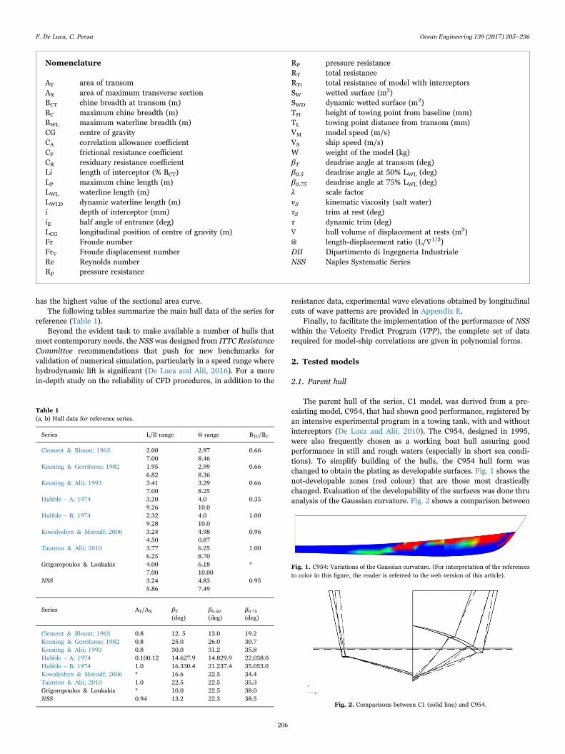
The parent hull of the series, C1 model, was derived from a pre-existing model, C954, that had shown good performance, registered byan intensive experimental program in a towing tank, with and withoutinterceptors (De Luca and Alii, 2010). The C954, designed in 1995,were also frequently chosen as a working boat hull assuring goodperformance in still and rough waters (especially in short sea condi-tions). To simplify building of the hulls, the C954 hull form waschanged to obtain the plating as developable surfaces. Fig. 1 shows thenot-developable zones (red colour) that are those most drasticallychanged. Evaluation of the developability of the surfaces was done thruanalysis of the Gaussian curvature. Fig. 2 shows a comparison between
Nomenclature
AT area of transomAX area of maximum transverse sectionBCT chine breadth at transom (m)BC maximum chine breadth (m)BWL maximum waterline breadth (m)CG centre of gravityCA correlation allowance coefficientCF frictional resistance coefficientCR residuary resistance coefficientLi length of interceptor (% BCT)LP maximum chine length (m)LWL waterline length (m)LWLD dynamic waterline length (m)i depth of interceptor (mm)iE half angle of entrance (deg)LCG longitudinal position of centre of gravity (m)Fr Froude numberFr∇ Froude displacement numberRe Reynolds numberRP pressure resistance
RP pressure resistanceRT total resistanceRTi total resistance of model with interceptorsSW wetted surface (m2)SWD dynamic wetted surface (m2)TH height of towing point from baseline (mm)TL towing point distance from transom (mm)VM model speed (m/s)VS ship speed (m/s)W weight of the model (kg)βT deadrise angle at transom (deg)β0.5 deadrise angle at 50% LWL (deg)β0.75 deadrise angle at 75% LWL (deg)λ scale factorνS kinematic viscosity (salt water)τS trim at rest (deg)τ dynamic trim (deg)∇ hull volume of displacement at rests (m3)Ⓜ length-displacement ratio (L/∇1/3)DII Dipartimento di Ingegneria IndustrialeNSS Naples Systematic Series
Fig. 1. C954: Variations of the Gaussian curvature. (For interpretation of the referencesto color in this figure, the reader is referred to the web version of this article).
Table 1(a, b) Hull data for reference series.
Series L/B range Ⓜ range BTC/BC
Clement & Blount; 1963 2.00 2.97 0.667.00 8.46
Keuning & Gerritsma; 1982 1.95 2.99 0.666.82 8.36
Keuning & Alii; 1993 3.41 3.29 0.667.00 8.25
Hubble – A; 1974 3.20 4.0 0.359.26 10.0
Hubble – B; 1974 2.32 4.0 1.009.28 10.0
Kowalyshyn & Metcalf; 2006 3.24 4.98 0.964.50 0.87
Taunton & Alii; 2010 3.77 6.25 1.006.25 8.70
Grigoropoulos & Loukakis 4.00 6.18 *7.00 10.00
NSS 3.24 4.83 0.955.86 7.49
Series AT/AX βT β0.50 β0.75(deg) (deg) (deg)
Clement & Blount; 1963 0.8 12. 5 13.0 19.2Keuning & Gerritsma; 1982 0.8 25.0 26.0 30.7Keuning & Alii; 1993 0.8 30.0 31.2 35.8Hubble – A; 1974 0.100.12 14.627.9 14.829.9 22.038.0Hubble – B; 1974 1.0 16.330.4 21.237.4 35.053.0Kowalyshyn & Metcalf; 2006 * 16.6 22.5 34.4Taunton & Alii; 2010 1.0 22.5 22.5 35.3Grigoropoulos & Loukakis * 10.0 22.5 38.0NSS 0.94 13.2 22.3 38.5
Fig. 2. Comparisons between C1 (solid line) and C954.
F. De Luca, C. Pensa Ocean Engineering 139 (2017) 205–236
206
the transversal sections of the C954 and C1 hulls and highlights thesubstantial identity of the C1 and C954 models.
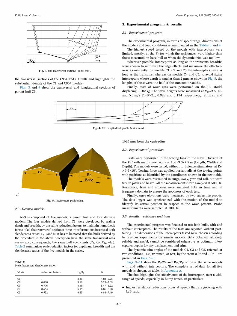
Figs. 3 and 4 show the transversal and longitudinal sections ofparent hull C1.
2.2. Derived models
NSS is composed of five models: a parent hull and four derivatemodels. The four models derived from C1, were developed by scalingdepth and breadth, by the same reduction factors, to maintain homotheticforms of all the transversal sections; these transformations increased bothslenderness ratios: L/B and Ⓜ. It has to be noted that the hulls derived bythe procedure in the above description have the same transversal areacurves and, consequently, the same hull coefficients (CB, CP, CW, etc.).Table 2 summarizes scale reduction factors for depth and breadth and theslenderness ratios of the five models in the series.
3. Experimental program & results
3.1. Experimental program
The experimental program, in terms of speed range, dimensions ofthe models and load conditions is summarized in the Tables 3 and 4.
The highest speed tested on the models with interceptors werelimited, mostly, at the Fr for which the resistances were higher thanthose measured on bare hull or when the dynamic trim was too low.
Wherever possible interceptors as long as the transoms breadthswere chosen to minimize the edge effects and maximize the effective-ness. Consistently, on models C1, C2 and C3 the interceptors were aslong as the transoms, whereas on models C4 and C5, to avoid fixinginterceptors whose depth is smaller than 2 mm, as shown in Fig. 5, thelengths of these were the half of the transom breadths.
Finally, tests of wave cuts were performed on the C2 Modeldisplacing 96.82 kg. The wave heights were measured at VM=3.5, 4.5and 5.5 m/s Fr=0.721, 0.928 and 1.134 respectively), at 1125 and
1625 mm from the centre-line.
3.2. Experimental procedure
Tests were performed in the towing tank of the Naval Division ofthe DII with main dimensions of 136×9.0×4.5 m (Length, Width andDepth). The models were tested, without turbulence stimulators, at Re> 3.5×10⁶. Towing force was applied horizontally at the towing pointswith positions as identified by the coordinates shown in the next table.
The models were restrained in surge, sway, yaw and roll, but werefree in pitch and heave. All the measurements were sampled at 500 Hz.Resistance, trim and sinkage were analyzed both in time and infrequency domain to assure the goodness of each test.
Finally, wave elevations were measured by two capacitive probes.The data logger was synchronized with the motion of the model toidentify its actual position in respect to the wave pattern. Probemeasurements were sampled at 100 Hz.
3.3. Results: resistance and trim
The experimental program was finalized to test both hulls, with andwithout interceptors. The results of the tests are reported without post-fairing. The dimensions of the interceptors tested were chosen accordingto previous experiments on similar models. Data obtained, althoughreliable and useful, cannot be considered exhaustive as optimum inter-ceptor's depths for any displacement and trim.
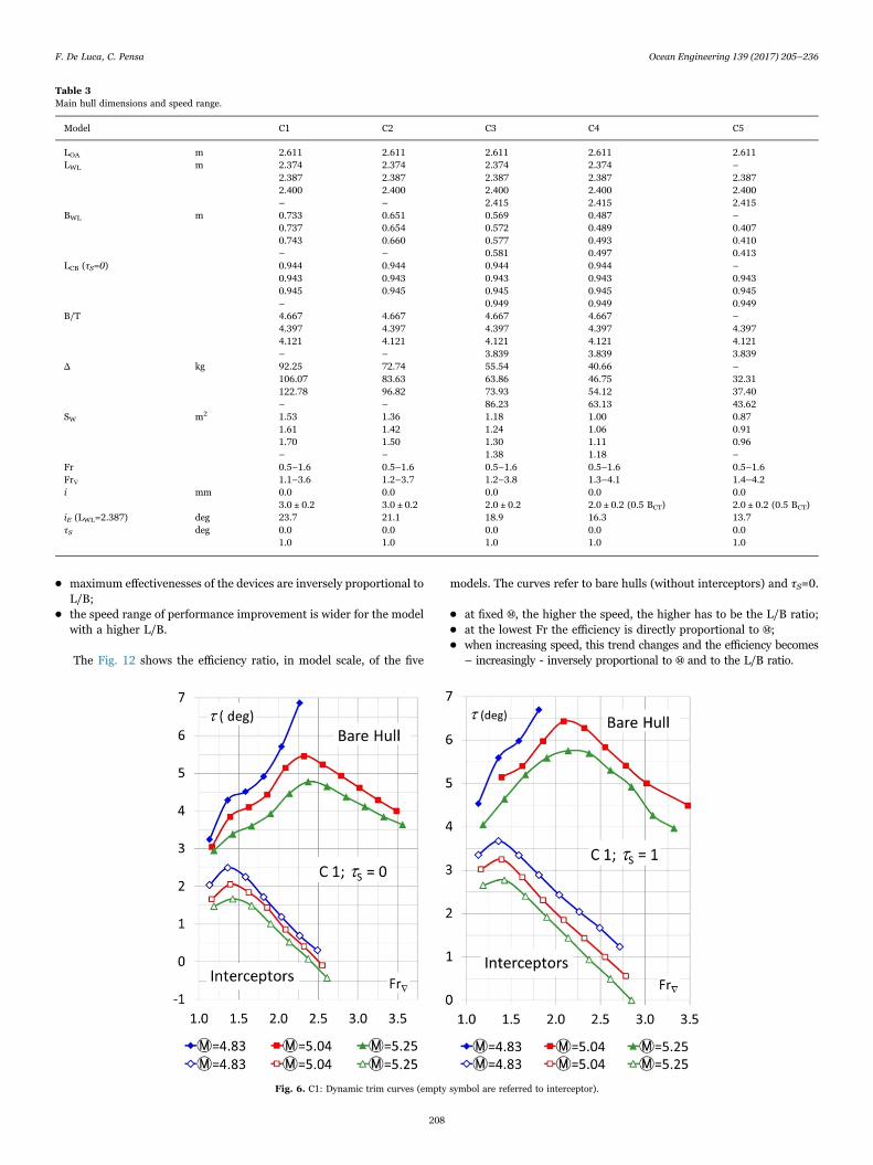
The dynamic trim angles of the models C1, C3 and C5, referred attwo conditions - i.e., trimmed, at rest, by the stern 0.0° and 1.0° – arepresented in Figs. 6–8.
Figs. 9–11 show the RT/W and RTi/RT ratios of the same modelswith and without interceptors. The complete set of data for all fivemodels is shown, as table, in Appendix A.
The data highlights the effectiveness of the interceptors over a widerange of speeds, especially in hump zones. In particular:
• higher resistance reductions occur at speeds that are growing withL/B ratio;
Fig. 3. C1: Transversal sections (units: mm).
Fig. 4. C1: Longitudinal profile (units: mm).
Fig. 5. Interceptors positioning.
Table 2Scale factors and slenderness ratios.
Model reduction factors LP/BC Ⓜ
C1 / 3.45 4.83–5.25C2 0.888 3.89 5.23–5.69C3 0.776 4.45 5.47–6.22C4 0.664 5.19 6.06–6.90C5 0.552 6.25 6.86–7.49
F. De Luca, C. Pensa Ocean Engineering 139 (2017) 205–236
207
• maximum effectivenesses of the devices are inversely proportional toL/B;
• the speed range of performance improvement is wider for the modelwith a higher L/B.
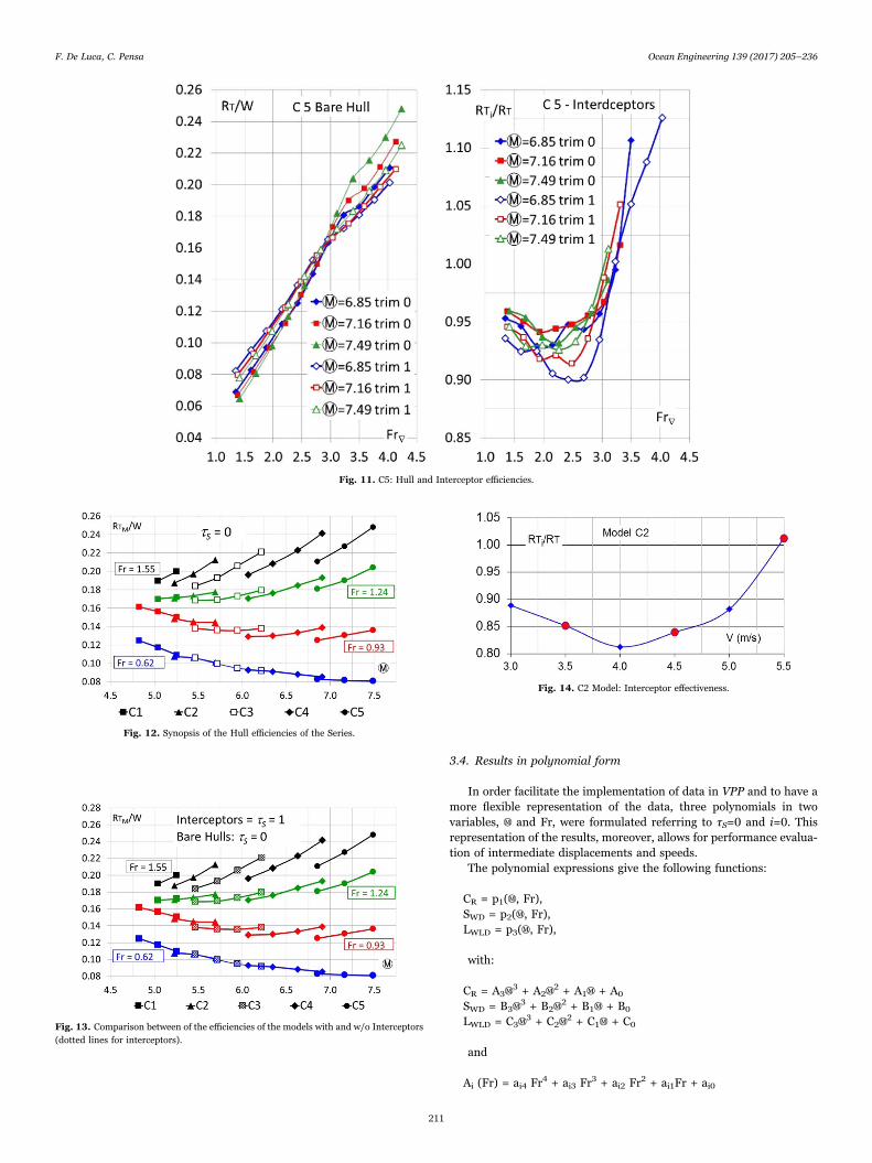
The Fig. 12 shows the efficiency ratio, in model scale, of the five
models. The curves refer to bare hulls (without interceptors) and τS=0.
• at fixed Ⓜ, the higher the speed, the higher has to be the L/B ratio;
• at the lowest Fr the efficiency is directly proportional to Ⓜ;
• when increasing speed, this trend changes and the efficiency becomes– increasingly - inversely proportional to Ⓜ and to the L/B ratio.
Fig. 6. C1: Dynamic trim curves (empty symbol are referred to interceptor).
Table 3Main hull dimensions and speed range.
Model C1 C2 C3 C4 C5
LOA m 2.611 2.611 2.611 2.611 2.611LWL m 2.374 2.374 2.374 2.374 –
2.387 2.387 2.387 2.387 2.3872.400 2.400 2.400 2.400 2.400– – 2.415 2.415 2.415
BWL m 0.733 0.651 0.569 0.487 –
0.737 0.654 0.572 0.489 0.4070.743 0.660 0.577 0.493 0.410– – 0.581 0.497 0.413
LCB (τS=0) 0.944 0.944 0.944 0.944 –
0.943 0.943 0.943 0.943 0.9430.945 0.945 0.945 0.945 0.945– 0.949 0.949 0.949
B/T 4.667 4.667 4.667 4.667 –
4.397 4.397 4.397 4.397 4.3974.121 4.121 4.121 4.121 4.121– – 3.839 3.839 3.839
Δ kg 92.25 72.74 55.54 40.66 –
106.07 83.63 63.86 46.75 32.31122.78 96.82 73.93 54.12 37.40– – 86.23 63.13 43.62
SW m2 1.53 1.36 1.18 1.00 0.871.61 1.42 1.24 1.06 0.911.70 1.50 1.30 1.11 0.96– – 1.38 1.18 –
Fr 0.5–1.6 0.5–1.6 0.5–1.6 0.5–1.6 0.5–1.6Fr∇ 1.1–3.6 1.2–3.7 1.2–3.8 1.3–4.1 1.4–4.2i mm 0.0 0.0 0.0 0.0 0.0
3.0 ± 0.2 3.0 ± 0.2 2.0 ± 0.2 2.0 ± 0.2 (0.5 BCT) 2.0 ± 0.2 (0.5 BCT)iΕ (LWL=2.387) deg 23.7 21.1 18.9 16.3 13.7τS deg 0.0 0.0 0.0 0.0 0.0
1.0 1.0 1.0 1.0 1.0
F. De Luca, C. Pensa Ocean Engineering 139 (2017) 205–236
208
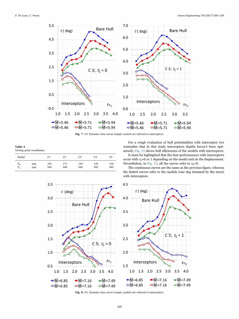
For a rough evaluation of hull potentialities with interceptor (weremember that in this study interceptors depths haven’t been opti-mized), Fig. 13 shows hull efficiencies of the models with interceptors.
It must be highlighted that the best performances with interceptorsoccur with τS=0 or 1 depending on the model and on the displacement.Nevertheless, in Fig. 13, all the curves refer to τS=0.
The continuous curves are the same as the previous figure, whereasthe dotted curves refer to the models (one deg trimmed by the stern)with interceptors.
Table 4Towing point coordinates.
Model C1 C2 C3 C4 C5
TH mm 191 171 154 145 134TL mm 945 945 945 945 945
Fig. 7. C3: Dynamic trim curves (empty symbol are referred to interceptor).
Fig. 8. C5: Dynamic trim curves (empty symbol are referred to interceptor).
F. De Luca, C. Pensa Ocean Engineering 139 (2017) 205–236
209
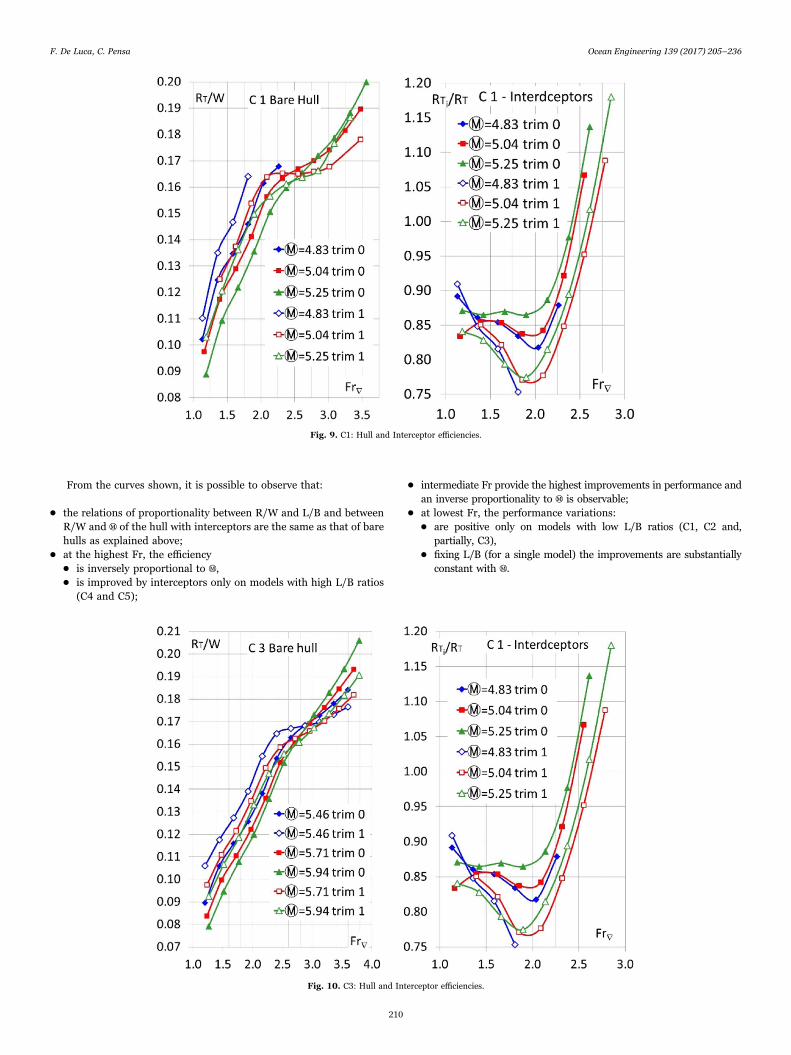
From the curves shown, it is possible to observe that:
• the relations of proportionality between R/W and L/B and betweenR/W and Ⓜ of the hull with interceptors are the same as that of barehulls as explained above;
• at the highest Fr, the efficiency
• is inversely proportional to Ⓜ,
• is improved by interceptors only on models with high L/B ratios(C4 and C5);
• intermediate Fr provide the highest improvements in performance andan inverse proportionality to Ⓜ is observable;
• at lowest Fr, the performance variations:
• are positive only on models with low L/B ratios (C1, C2 and,partially, C3),
• fixing L/B (for a single model) the improvements are substantiallyconstant with Ⓜ.
Fig. 9. C1: Hull and Interceptor efficiencies.
Fig. 10. C3: Hull and Interceptor efficiencies.
F. De Luca, C. Pensa Ocean Engineering 139 (2017) 205–236
210
3.4. Results in polynomial form
In order facilitate the implementation of data in VPP and to have amore flexible representation of the data, three polynomials in twovariables, Ⓜ and Fr, were formulated referring to τS=0 and i=0. Thisrepresentation of the results, moreover, allows for performance evalua-tion of intermediate displacements and speeds.
The polynomial expressions give the following functions:
CR = p1(Ⓜ, Fr),SWD = p2(Ⓜ, Fr),LWLD = p3(Ⓜ, Fr),
with:
CR = A3Ⓜ3 + A2Ⓜ
2 + A1Ⓜ + A0
SWD = B3Ⓜ3 + B2Ⓜ
2 + B1Ⓜ + B0
LWLD = C3Ⓜ3 + C2Ⓜ
2 + C1Ⓜ + C0
and
Ai (Fr) = ai4 Fr4 + ai3 Fr3 + ai2 Fr2 + ai1Fr + ai0
Fig. 12. Synopsis of the Hull efficiencies of the Series.
Fig. 13. Comparison between of the efficiencies of the models with and w/o Interceptors(dotted lines for interceptors).
Fig. 14. C2 Model: Interceptor effectiveness.
Fig. 11. C5: Hull and Interceptor efficiencies.
F. De Luca, C. Pensa Ocean Engineering 139 (2017) 205–236
211
Bi (Fr) = bi4 Fr4 + bi3 Fr3 + bi2 Fr2 + bi1Fr + bi0Ci (Fr) = ci4 Fr4 + ci3 Fr3 + ci2 Fr2 + ci1Fr + ci0
Due to the great number of coefficients, the polynomial formulas,for convenience, will be expressed with the vectors and the matrices asdefined below:
(Fr)T = {1, Fr, Fr2, Fr3, Fr4};ⓂT = {1, Ⓜ, Ⓜ 2, Ⓜ 3};
whereby the polynomials can be expressed as the product of thevectors: Fr and Ⓜ for the matrices A, B and C.
CR = (Fr)T·A Ⓜ
SWD = (Fr)T·B Ⓜ
LWLD = (Fr)T·C Ⓜ
In addition to the capability to predict resistance at intermediatespeed and displacements, the supply of data as continuous functionsallows, in the development of the project, to evaluate the sensibility ofresistance respect Ⓜ (i.e., the weight) that is the most affected byuncertainty in the development of a project. Indeed, the continuouspolynomial functions allow an easy evaluation of a partial derivativethrough the use of the same coefficients. Defining
Ⓜ iT = {0, 1, 2Ⓜ, 3Ⓜ 2, 4Ⓜ 3, 5Ⓜ4}
it is possible to evaluate the partial derivative of CR, SWD and LWLD
to Ⓜ as follows:
∂CR/∂Ⓜ = (Fr)T·A Ⓜ i
∂SWD/∂Ⓜ = (Fr)T·B Ⓜi
∂LWLD/∂Ⓜ = (Fr)T·C Ⓜi
This is quite useful by providing an evaluation of error propagationon resistance due to Ⓜ.
δCR (Ⓜ) = |∂CR/∂Ⓜ|δⓂ
In short, in this way the designer can estimate the maximum errorfor resistance due to the error expected in Ⓜ which, especially in thefirst part of design, could be significant. Similarly, it is possible toevaluate the expression of the partial derivatives of Fr to appraise thesensitivity of the resistance to the speed.
The coefficients of the matrices have been obtained by applying aleast-squares root fit procedure to the numerical results, similar to theoptimization techniques used to find a set of design parameters, asdescribed in Balsamo and Alii (2011).
3.5. Results: wave elevations
The curves shown in Appendix E highlight a noticeable reduction ofthe wave heights due to the work of the interceptors and the directproportionality between wave heights and speed. It is of interest toobserve that the effectiveness of the interceptors, as shown in Fig. 14,do not follow the same proportionality.
This circumstance shows that at higher speeds, the frictionalresistance, as a component of the total resistance, increases its weightin respect to wave pattern resistance. This higher weight of thefrictional resistance is due to a larger wetted surface induced by thelower trim effected by the interceptors. Consequently, to evaluateactual interceptor effectiveness, this must be referred to in theresistances at full scale, otherwise, in model scale the interceptor'seffectiveness will be underestimated.
3.6. Model-Ship correlation
To make feasible model-ship correlations following ITTC recom-mendations, wetted lengths and surfaces of the models underway werereported for each test in Appendix A. To determine wetted surfaces, theboundaries of these surfaces were evaluated by camera documentationand assigned to hull surfaces in 3D-CAD. The identified surfacesinclude the reattached wetted area above the chines. Whisker sprayareas, as a precaution, were excluded from the estimations of thewetted surfaces due to the uncertainty of their contribution to viscousresistance. With the same criterion of precaution, the dynamic wettedlength taken into account for the Reynolds number was measured onthe keel line (not as an average value between keel and chine lengths).
4. Conclusions & future work
This work presented a new hard chine Systematic Series, composedof five models, showing hull forms, geometric coefficients and a table ofoffset. The hull forms of the models were characterized by a very highlevel of developability of the plating. In tabular form and as acontinuous function, CR and dynamic SW and LWL are furnished tocarry out very accurate model-ship correlations. The experimental testshighlight the good quality of the parent hull and show it to be in linewith state-of-the-art technologies.
The experimental program on the Series is in progress to char-acterize the behaviour of the models on waves and to evaluate, for eachmodel, the dependence on the interceptor effectiveness of the depth i.To the completion of the study on the models with interceptors, data inpolynomial form will be furnished as done for the bare hulls.
Both these tests will be completed at the end of the 2017.
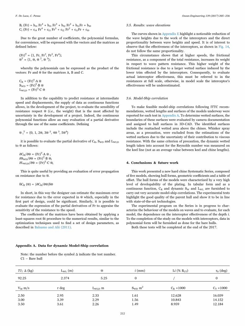
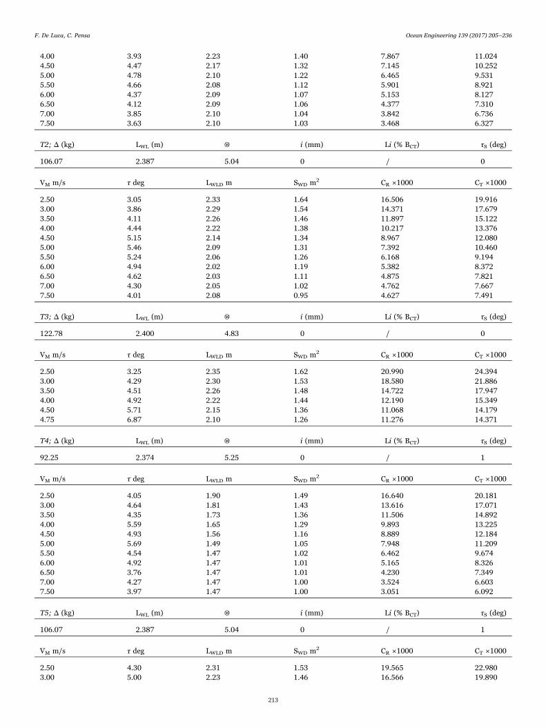
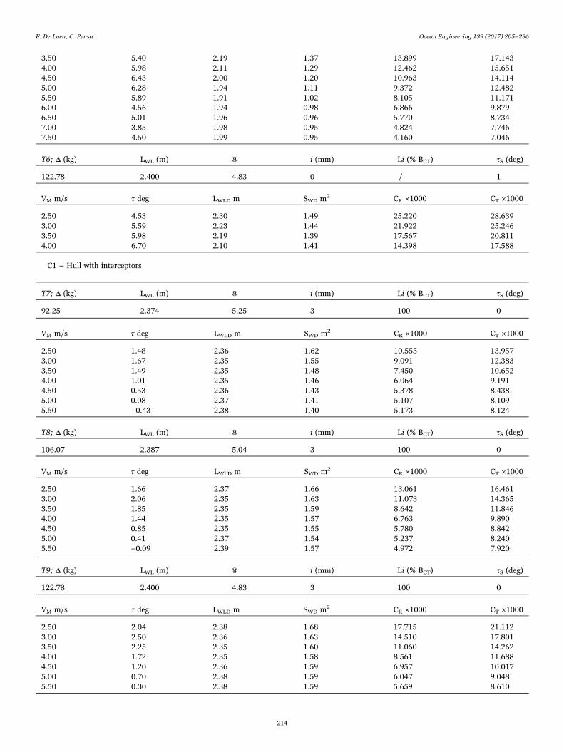
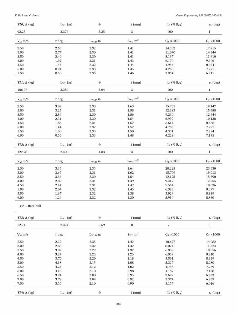
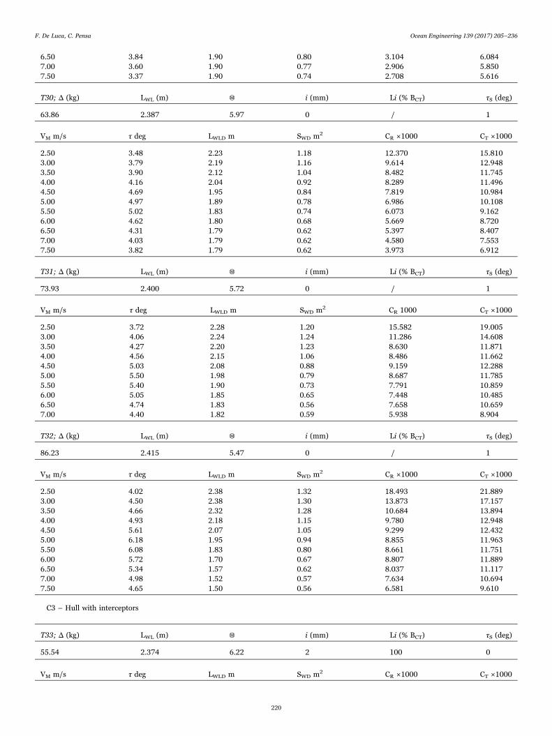
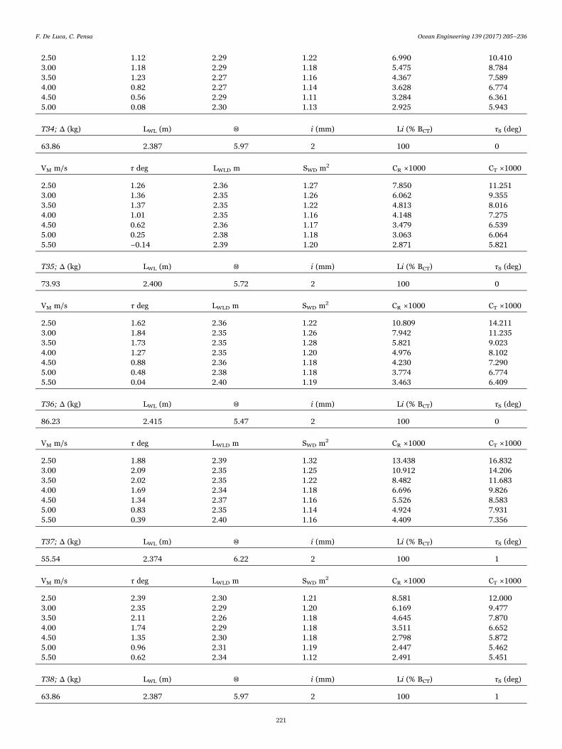
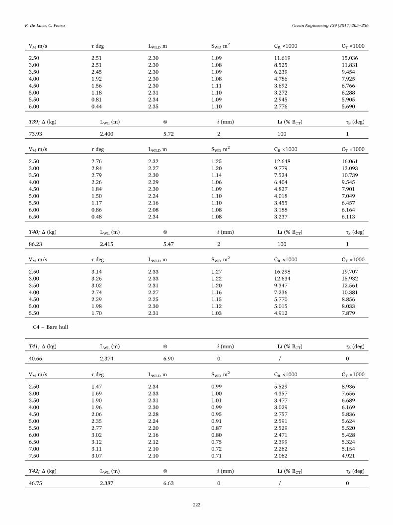
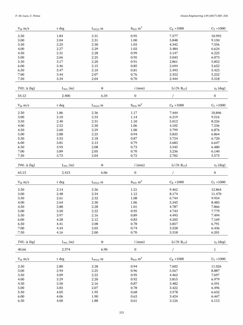
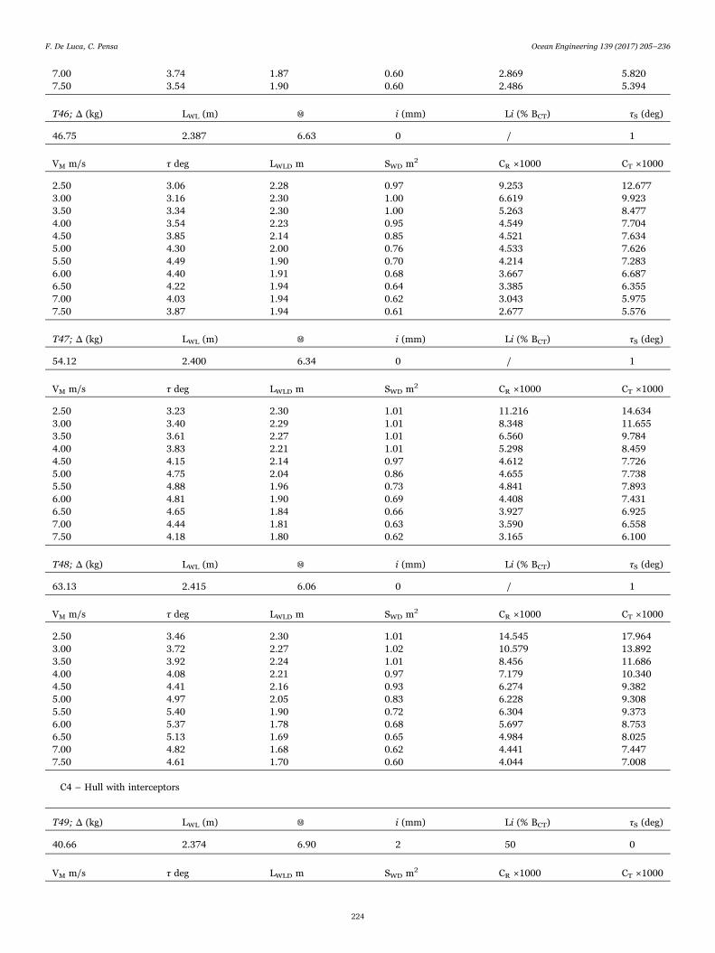
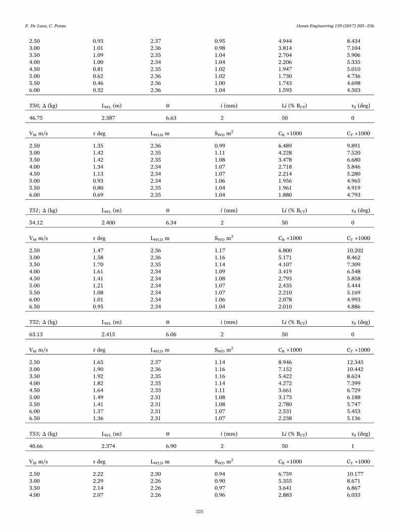
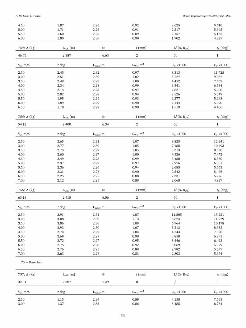
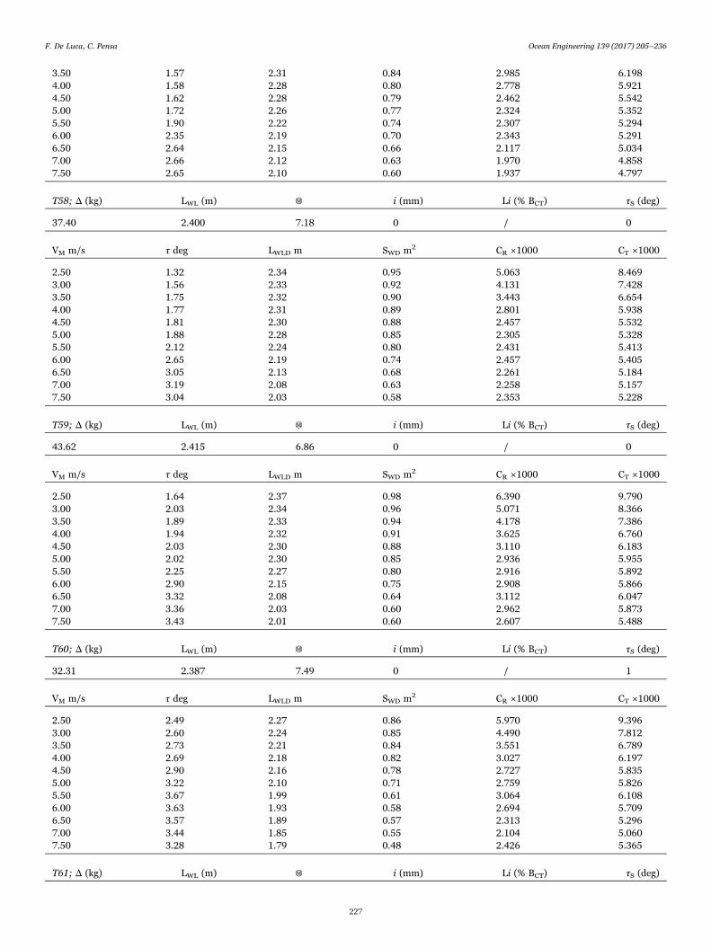
Appendix A. Data for dynamic Model-Ship correlation
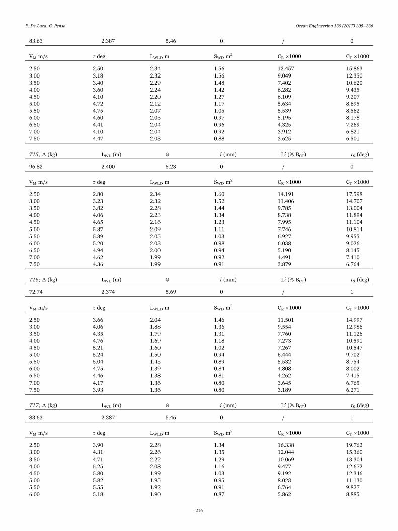
Note: the number before the symbol Δ indicate the test number.C1 – Bare hull
Τ1; Δ (kg) LWL (m) Ⓜ i (mm) Li (% BCT) τS (deg)
92.25 2.374 5.25 0 / 0
VM m/s τ deg LWLD m SWD m2 CR ×1000 CT ×1000
2.50 2.95 2.33 1.61 12.628 16.0393.00 3.39 2.29 1.56 10.843 14.1523.50 3.61 2.26 1.49 8.959 12.184
F. De Luca, C. Pensa Ocean Engineering 139 (2017) 205–236
212
4.00 3.93 2.23 1.40 7.867 11.0244.50 4.47 2.17 1.32 7.145 10.2525.00 4.78 2.10 1.22 6.465 9.5315.50 4.66 2.08 1.12 5.901 8.9216.00 4.37 2.09 1.07 5.153 8.1276.50 4.12 2.09 1.06 4.377 7.3107.00 3.85 2.10 1.04 3.842 6.7367.50 3.63 2.10 1.03 3.468 6.327
Τ2; Δ (kg) LWL (m) Ⓜ i (mm) Li (% BCT) τS (deg)
106.07 2.387 5.04 0 / 0
VM m/s τ deg LWLD m SWD m2 CR ×1000 CT ×1000
2.50 3.05 2.33 1.64 16.506 19.9163.00 3.86 2.29 1.54 14.371 17.6793.50 4.11 2.26 1.46 11.897 15.1224.00 4.44 2.22 1.38 10.217 13.3764.50 5.15 2.14 1.34 8.967 12.0805.00 5.46 2.09 1.31 7.392 10.4605.50 5.24 2.06 1.26 6.168 9.1946.00 4.94 2.02 1.19 5.382 8.3726.50 4.62 2.03 1.11 4.875 7.8217.00 4.30 2.05 1.02 4.762 7.6677.50 4.01 2.08 0.95 4.627 7.491
Τ3; Δ (kg) LWL (m) Ⓜ i (mm) Li (% BCT) τS (deg)
122.78 2.400 4.83 0 / 0
VM m/s τ deg LWLD m SWD m2 CR ×1000 CT ×1000
2.50 3.25 2.35 1.62 20.990 24.3943.00 4.29 2.30 1.53 18.580 21.8863.50 4.51 2.26 1.48 14.722 17.9474.00 4.92 2.22 1.44 12.190 15.3494.50 5.71 2.15 1.36 11.068 14.1794.75 6.87 2.10 1.26 11.276 14.371
Τ4; Δ (kg) LWL (m) Ⓜ i (mm) Li (% BCT) τS (deg)
92.25 2.374 5.25 0 / 1
VM m/s τ deg LWLD m SWD m2 CR ×1000 CT ×1000
2.50 4.05 1.90 1.49 16.640 20.1813.00 4.64 1.81 1.43 13.616 17.0713.50 4.35 1.73 1.36 11.506 14.8924.00 5.59 1.65 1.29 9.893 13.2254.50 4.93 1.56 1.16 8.889 12.1845.00 5.69 1.49 1.05 7.948 11.2095.50 4.54 1.47 1.02 6.462 9.6746.00 4.92 1.47 1.01 5.165 8.3266.50 3.76 1.47 1.01 4.230 7.3497.00 4.27 1.47 1.00 3.524 6.6037.50 3.97 1.47 1.00 3.051 6.092
Τ5; Δ (kg) LWL (m) Ⓜ i (mm) Li (% BCT) τS (deg)
106.07 2.387 5.04 0 / 1
VM m/s τ deg LWLD m SWD m2 CR ×1000 CT ×1000
2.50 4.30 2.31 1.53 19.565 22.9803.00 5.00 2.23 1.46 16.566 19.890
F. De Luca, C. Pensa Ocean Engineering 139 (2017) 205–236
213
3.50 5.40 2.19 1.37 13.899 17.1434.00 5.98 2.11 1.29 12.462 15.6514.50 6.43 2.00 1.20 10.963 14.1145.00 6.28 1.94 1.11 9.372 12.4825.50 5.89 1.91 1.02 8.105 11.1716.00 4.56 1.94 0.98 6.866 9.8796.50 5.01 1.96 0.96 5.770 8.7347.00 3.85 1.98 0.95 4.824 7.7467.50 4.50 1.99 0.95 4.160 7.046
Τ6; Δ (kg) LWL (m) Ⓜ i (mm) Li (% BCT) τS (deg)
122.78 2.400 4.83 0 / 1
VM m/s τ deg LWLD m SWD m2 CR ×1000 CT ×1000
2.50 4.53 2.30 1.49 25.220 28.6393.00 5.59 2.23 1.44 21.922 25.2463.50 5.98 2.19 1.39 17.567 20.8114.00 6.70 2.10 1.41 14.398 17.588
C1 – Hull with interceptors
Τ7; Δ (kg) LWL (m) Ⓜ i (mm) Li (% BCT) τS (deg)
92.25 2.374 5.25 3 100 0
VM m/s τ deg LWLD m SWD m2 CR ×1000 CT ×1000
2.50 1.48 2.36 1.62 10.555 13.9573.00 1.67 2.35 1.55 9.091 12.3833.50 1.49 2.35 1.48 7.450 10.6524.00 1.01 2.35 1.46 6.064 9.1914.50 0.53 2.36 1.43 5.378 8.4385.00 0.08 2.37 1.41 5.107 8.1095.50 −0.43 2.38 1.40 5.173 8.124
Τ8; Δ (kg) LWL (m) Ⓜ i (mm) Li (% BCT) τS (deg)
106.07 2.387 5.04 3 100 0
VM m/s τ deg LWLD m SWD m2 CR ×1000 CT ×1000
2.50 1.66 2.37 1.66 13.061 16.4613.00 2.06 2.35 1.63 11.073 14.3653.50 1.85 2.35 1.59 8.642 11.8464.00 1.44 2.35 1.57 6.763 9.8904.50 0.85 2.35 1.55 5.780 8.8425.00 0.41 2.37 1.54 5.237 8.2405.50 −0.09 2.39 1.57 4.972 7.920
Τ9; Δ (kg) LWL (m) Ⓜ i (mm) Li (% BCT) τS (deg)
122.78 2.400 4.83 3 100 0
VM m/s τ deg LWLD m SWD m2 CR ×1000 CT ×1000
2.50 2.04 2.38 1.68 17.715 21.1123.00 2.50 2.36 1.63 14.510 17.8013.50 2.25 2.35 1.60 11.060 14.2624.00 1.72 2.35 1.58 8.561 11.6884.50 1.20 2.36 1.59 6.957 10.0175.00 0.70 2.38 1.59 6.047 9.0485.50 0.30 2.38 1.59 5.659 8.610
F. De Luca, C. Pensa Ocean Engineering 139 (2017) 205–236
214
Τ10; Δ (kg) LWL (m) Ⓜ i (mm) Li (% BCT) τS (deg)
92.25 2.374 5.25 3 100 1
VM m/s τ deg LWLD m SWD m2 CR ×1000 CT ×1000
2.50 2.65 2.32 1.41 14.502 17.9153.00 2.77 2.30 1.41 11.040 14.3443.50 2.40 2.30 1.41 8.197 11.4104.00 1.92 2.31 1.43 6.170 9.3064.50 1.44 2.32 1.44 4.954 8.0245.00 0.94 2.33 1.45 4.280 7.2915.50 0.50 2.35 1.46 3.954 6.911
Τ11; Δ (kg) LWL (m) Ⓜ i (mm) Li (% BCT) τS (deg)
106.07 2.387 5.04 3 100 1
VM m/s τ deg LWLD m SWD m2 CR ×1000 CT ×1000
2.50 3.02 2.33 1.63 15.735 19.1473.00 3.25 2.31 1.58 12.383 15.6883.50 2.84 2.30 1.56 9.230 12.4444.00 2.31 2.30 1.54 6.999 10.1384.50 1.85 2.31 1.52 5.614 8.6865.00 1.44 2.32 1.52 4.783 7.7975.50 1.00 2.33 1.50 4.331 7.2946.00 0.56 2.33 1.48 4.228 7.145
Τ12; Δ (kg) LWL (m) Ⓜ i (mm) Li (% BCT) τS (deg)
122.78 2.400 4.83 3 100 1
VM m/s τ deg LWLD m SWD m2 CR ×1000 CT ×1000
2.50 3.35 2.35 1.64 20.225 23.6303.00 3.67 2.31 1.62 15.709 19.0133.50 3.34 2.30 1.54 12.175 15.3904.00 2.89 2.31 1.49 9.417 12.5554.50 2.44 2.31 1.47 7.564 10.6365.00 2.04 2.32 1.45 6.383 9.3975.50 1.67 2.32 1.38 5.924 8.8896.00 1.24 2.32 1.30 5.910 8.830
C2 – Bare hull
Τ13; Δ (kg) LWL (m) Ⓜ i (mm) Li (% BCT) τS (deg)
72.74 2.374 5.69 0 / 0
VM m/s τ deg LWLD m SWD m2 CR ×1000 CT ×1000
2.50 2.22 2.35 1.42 10.677 14.0823.00 2.83 2.32 1.42 8.024 11.3243.50 3.07 2.29 1.32 6.839 10.0564.00 3.24 2.25 1.25 6.059 9.2104.50 3.70 2.20 1.18 5.531 8.6295.00 4.18 2.15 1.08 5.227 8.2805.50 4.24 2.12 1.02 4.758 7.7696.00 4.13 2.10 0.98 4.187 7.1586.50 3.94 2.08 0.95 3.699 6.6337.00 3.78 2.09 0.92 3.374 6.2697.50 3.56 2.10 0.90 3.157 6.016
Τ14; Δ (kg) LWL (m) Ⓜ i (mm) Li (% BCT) τS (deg)
F. De Luca, C. Pensa Ocean Engineering 139 (2017) 205–236
215
83.63 2.387 5.46 0 / 0
VM m/s τ deg LWLD m SWD m2 CR ×1000 CT ×1000
2.50 2.50 2.34 1.56 12.457 15.8633.00 3.18 2.32 1.56 9.049 12.3503.50 3.40 2.29 1.48 7.402 10.6204.00 3.60 2.24 1.42 6.282 9.4354.50 4.10 2.20 1.27 6.109 9.2075.00 4.72 2.12 1.17 5.634 8.6955.50 4.75 2.07 1.05 5.539 8.5626.00 4.60 2.05 0.97 5.195 8.1786.50 4.41 2.04 0.96 4.325 7.2697.00 4.10 2.04 0.92 3.912 6.8217.50 4.47 2.03 0.88 3.625 6.501
Τ15; Δ (kg) LWL (m) Ⓜ i (mm) Li (% BCT) τS (deg)
96.82 2.400 5.23 0 / 0
VM m/s τ deg LWLD m SWD m2 CR ×1000 CT ×1000
2.50 2.80 2.34 1.60 14.191 17.5983.00 3.23 2.32 1.52 11.406 14.7073.50 3.82 2.28 1.44 9.785 13.0044.00 4.06 2.23 1.34 8.738 11.8944.50 4.65 2.16 1.23 7.995 11.1045.00 5.37 2.09 1.11 7.746 10.8145.50 5.39 2.05 1.03 6.927 9.9556.00 5.20 2.03 0.98 6.038 9.0266.50 4.94 2.00 0.94 5.190 8.1457.00 4.62 1.99 0.92 4.491 7.4107.50 4.36 1.99 0.91 3.879 6.764
Τ16; Δ (kg) LWL (m) Ⓜ i (mm) Li (% BCT) τS (deg)
72.74 2.374 5.69 0 / 1
VM m/s τ deg LWLD m SWD m2 CR ×1000 CT ×1000
2.50 3.66 2.04 1.46 11.501 14.9973.00 4.06 1.88 1.36 9.554 12.9863.50 4.35 1.79 1.31 7.760 11.1264.00 4.76 1.69 1.18 7.273 10.5914.50 5.21 1.60 1.02 7.267 10.5475.00 5.24 1.50 0.94 6.444 9.7025.50 5.04 1.45 0.89 5.532 8.7546.00 4.75 1.39 0.84 4.808 8.0026.50 4.46 1.38 0.81 4.262 7.4157.00 4.17 1.36 0.80 3.645 6.7657.50 3.93 1.36 0.80 3.189 6.271
Τ17; Δ (kg) LWL (m) Ⓜ i (mm) Li (% BCT) τS (deg)
83.63 2.387 5.46 0 / 1
VM m/s τ deg LWLD m SWD m2 CR ×1000 CT ×1000
2.50 3.90 2.28 1.34 16.338 19.7623.00 4.31 2.26 1.35 12.044 15.3603.50 4.71 2.22 1.29 10.069 13.3044.00 5.25 2.08 1.16 9.477 12.6724.50 5.80 1.99 1.03 9.192 12.3465.00 5.82 1.95 0.95 8.023 11.1305.50 5.55 1.92 0.91 6.764 9.8276.00 5.18 1.90 0.87 5.862 8.885
F. De Luca, C. Pensa Ocean Engineering 139 (2017) 205–236
216
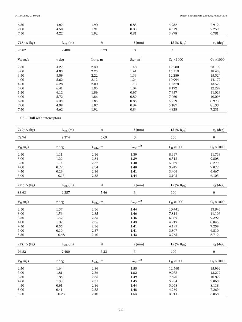
6.50 4.82 1.90 0.85 4.932 7.9127.00 4.50 1.91 0.83 4.319 7.2597.50 4.22 1.92 0.81 3.878 6.781
Τ18; Δ (kg) LWL (m) Ⓜ i (mm) Li (% BCT) τS (deg)
96.82 2.400 5.23 0 / 1
VM m/s τ deg LWLD m SWD m2 CR ×1000 CT ×1000
2.50 4.27 2.30 1.48 19.780 23.1993.00 4.83 2.25 1.41 15.119 18.4383.50 5.09 2.22 1.33 12.289 15.5244.00 5.62 2.12 1.24 10.994 14.1794.50 6.28 2.00 1.13 10.378 13.5295.00 6.41 1.95 1.04 9.192 12.2995.50 6.12 1.89 0.97 7.957 11.0296.00 5.72 1.86 0.89 7.060 10.0936.50 5.34 1.85 0.86 5.979 8.9737.00 4.99 1.87 0.84 5.187 8.1387.50 4.62 1.92 0.84 4.328 7.231
C2 – Hull with interceptors
Τ19; Δ (kg) LWL (m) Ⓜ i (mm) Li (% BCT) τS (deg)
72.74 2.374 5.69 3 100 0
VM m/s τ deg LWLD m SWD m2 CR ×1000 CT ×1000
2.50 1.11 2.36 1.39 8.337 11.7393.00 1.22 2.34 1.39 6.512 9.8083.50 1.14 2.32 1.40 5.069 8.2794.00 0.77 2.34 1.40 3.947 7.0774.50 0.29 2.36 1.41 3.406 6.4675.00 −0.15 2.38 1.44 3.105 6.105
Τ20; Δ (kg) LWL (m) Ⓜ i (mm) Li (% BCT) τS (deg)
83.63 2.387 5.46 3 100 0
VM m/s τ deg LWLD m SWD m2 CR ×1000 CT ×1000
2.50 1.37 2.36 1.44 10.441 13.8433.00 1.56 2.35 1.46 7.814 11.1063.50 1.52 2.35 1.46 6.089 9.2924.00 1.02 2.35 1.43 4.919 8.0454.50 0.55 2.36 1.41 4.199 7.2595.00 0.10 2.37 1.41 3.807 6.8105.50 −0.48 2.40 1.43 3.765 6.712
Τ21; Δ (kg) LWL (m) Ⓜ i (mm) Li (% BCT) τS (deg)
96.82 2.400 5.23 3 100 0
VM m/s τ deg LWLD m SWD m2 CR ×1000 CT ×1000
2.50 1.64 2.36 1.55 12.560 15.9623.00 1.81 2.36 1.52 9.988 13.2793.50 1.86 2.35 1.49 7.670 10.8724.00 1.33 2.35 1.45 5.934 9.0604.50 0.91 2.36 1.44 5.058 8.1185.00 0.41 2.38 1.48 4.269 7.2695.50 −0.23 2.40 1.54 3.911 6.858
F. De Luca, C. Pensa Ocean Engineering 139 (2017) 205–236
217
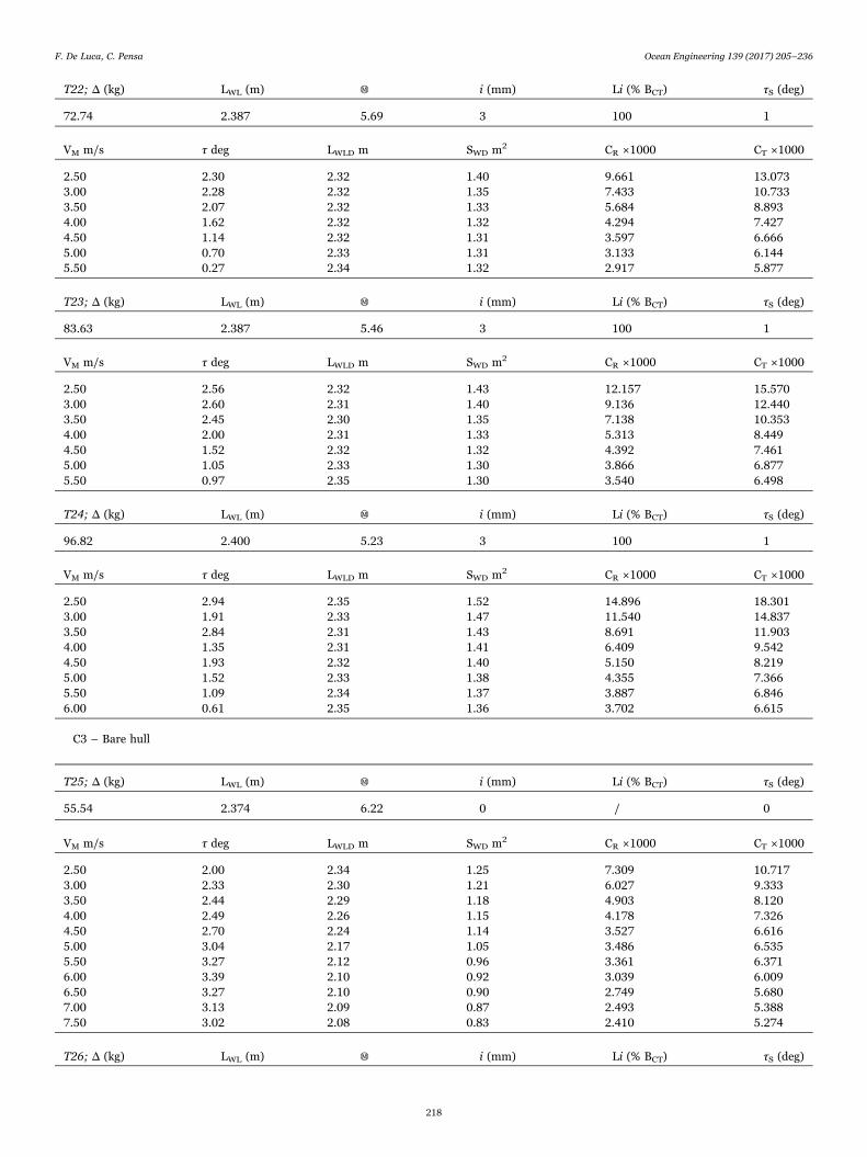
Τ22; Δ (kg) LWL (m) Ⓜ i (mm) Li (% BCT) τS (deg)
72.74 2.387 5.69 3 100 1
VM m/s τ deg LWLD m SWD m2 CR ×1000 CT ×1000
2.50 2.30 2.32 1.40 9.661 13.0733.00 2.28 2.32 1.35 7.433 10.7333.50 2.07 2.32 1.33 5.684 8.8934.00 1.62 2.32 1.32 4.294 7.4274.50 1.14 2.32 1.31 3.597 6.6665.00 0.70 2.33 1.31 3.133 6.1445.50 0.27 2.34 1.32 2.917 5.877
Τ23; Δ (kg) LWL (m) Ⓜ i (mm) Li (% BCT) τS (deg)
83.63 2.387 5.46 3 100 1
VM m/s τ deg LWLD m SWD m2 CR ×1000 CT ×1000
2.50 2.56 2.32 1.43 12.157 15.5703.00 2.60 2.31 1.40 9.136 12.4403.50 2.45 2.30 1.35 7.138 10.3534.00 2.00 2.31 1.33 5.313 8.4494.50 1.52 2.32 1.32 4.392 7.4615.00 1.05 2.33 1.30 3.866 6.8775.50 0.97 2.35 1.30 3.540 6.498
Τ24; Δ (kg) LWL (m) Ⓜ i (mm) Li (% BCT) τS (deg)
96.82 2.400 5.23 3 100 1
VM m/s τ deg LWLD m SWD m2 CR ×1000 CT ×1000
2.50 2.94 2.35 1.52 14.896 18.3013.00 1.91 2.33 1.47 11.540 14.8373.50 2.84 2.31 1.43 8.691 11.9034.00 1.35 2.31 1.41 6.409 9.5424.50 1.93 2.32 1.40 5.150 8.2195.00 1.52 2.33 1.38 4.355 7.3665.50 1.09 2.34 1.37 3.887 6.8466.00 0.61 2.35 1.36 3.702 6.615
C3 – Bare hull
Τ25; Δ (kg) LWL (m) Ⓜ i (mm) Li (% BCT) τS (deg)
55.54 2.374 6.22 0 / 0
VM m/s τ deg LWLD m SWD m2 CR ×1000 CT ×1000
2.50 2.00 2.34 1.25 7.309 10.7173.00 2.33 2.30 1.21 6.027 9.3333.50 2.44 2.29 1.18 4.903 8.1204.00 2.49 2.26 1.15 4.178 7.3264.50 2.70 2.24 1.14 3.527 6.6165.00 3.04 2.17 1.05 3.486 6.5355.50 3.27 2.12 0.96 3.361 6.3716.00 3.39 2.10 0.92 3.039 6.0096.50 3.27 2.10 0.90 2.749 5.6807.00 3.13 2.09 0.87 2.493 5.3887.50 3.02 2.08 0.83 2.410 5.274
Τ26; Δ (kg) LWL (m) Ⓜ i (mm) Li (% BCT) τS (deg)
F. De Luca, C. Pensa Ocean Engineering 139 (2017) 205–236
218
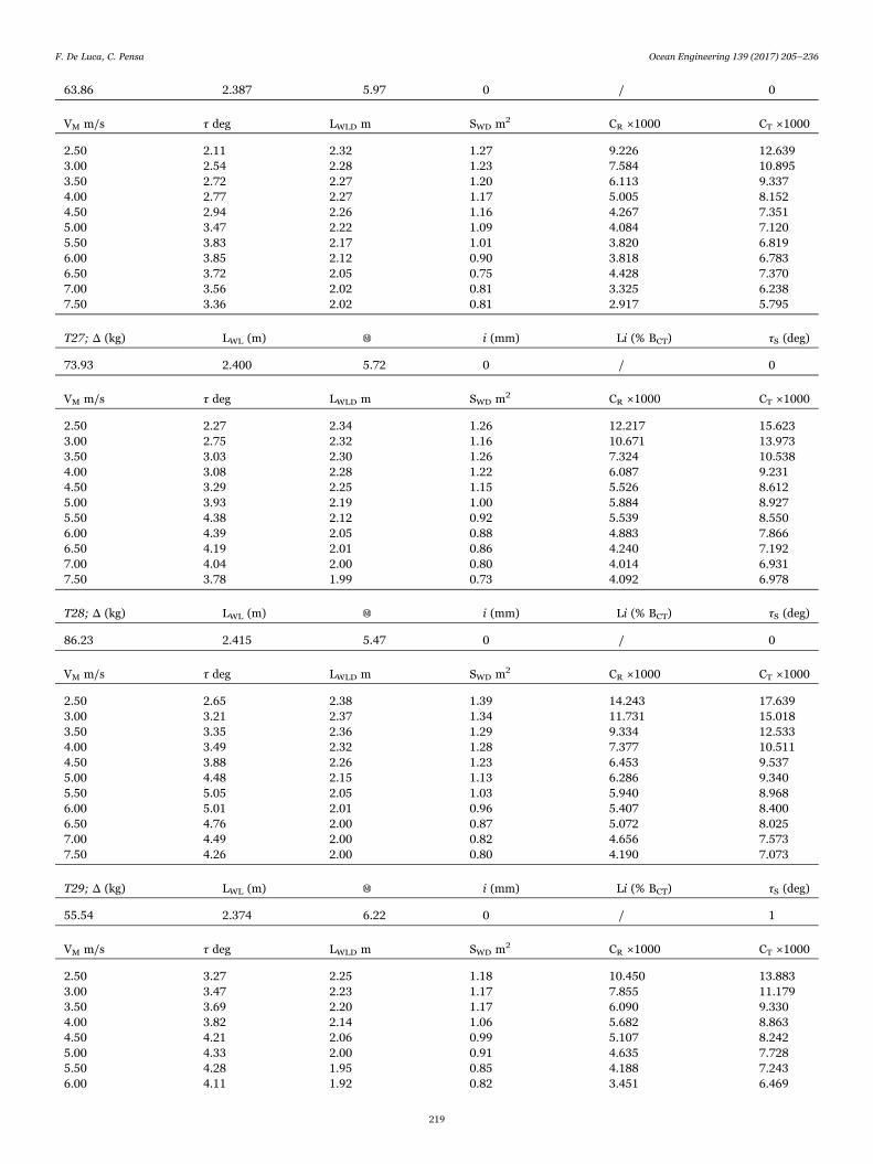
63.86 2.387 5.97 0 / 0
VM m/s τ deg LWLD m SWD m2 CR ×1000 CT ×1000
2.50 2.11 2.32 1.27 9.226 12.6393.00 2.54 2.28 1.23 7.584 10.8953.50 2.72 2.27 1.20 6.113 9.3374.00 2.77 2.27 1.17 5.005 8.1524.50 2.94 2.26 1.16 4.267 7.3515.00 3.47 2.22 1.09 4.084 7.1205.50 3.83 2.17 1.01 3.820 6.8196.00 3.85 2.12 0.90 3.818 6.7836.50 3.72 2.05 0.75 4.428 7.3707.00 3.56 2.02 0.81 3.325 6.2387.50 3.36 2.02 0.81 2.917 5.795
Τ27; Δ (kg) LWL (m) Ⓜ i (mm) Li (% BCT) τS (deg)
73.93 2.400 5.72 0 / 0
VM m/s τ deg LWLD m SWD m2 CR ×1000 CT ×1000
2.50 2.27 2.34 1.26 12.217 15.6233.00 2.75 2.32 1.16 10.671 13.9733.50 3.03 2.30 1.26 7.324 10.5384.00 3.08 2.28 1.22 6.087 9.2314.50 3.29 2.25 1.15 5.526 8.6125.00 3.93 2.19 1.00 5.884 8.9275.50 4.38 2.12 0.92 5.539 8.5506.00 4.39 2.05 0.88 4.883 7.8666.50 4.19 2.01 0.86 4.240 7.1927.00 4.04 2.00 0.80 4.014 6.9317.50 3.78 1.99 0.73 4.092 6.978
Τ28; Δ (kg) LWL (m) Ⓜ i (mm) Li (% BCT) τS (deg)
86.23 2.415 5.47 0 / 0
VM m/s τ deg LWLD m SWD m2 CR ×1000 CT ×1000
2.50 2.65 2.38 1.39 14.243 17.6393.00 3.21 2.37 1.34 11.731 15.0183.50 3.35 2.36 1.29 9.334 12.5334.00 3.49 2.32 1.28 7.377 10.5114.50 3.88 2.26 1.23 6.453 9.5375.00 4.48 2.15 1.13 6.286 9.3405.50 5.05 2.05 1.03 5.940 8.9686.00 5.01 2.01 0.96 5.407 8.4006.50 4.76 2.00 0.87 5.072 8.0257.00 4.49 2.00 0.82 4.656 7.5737.50 4.26 2.00 0.80 4.190 7.073
Τ29; Δ (kg) LWL (m) Ⓜ i (mm) Li (% BCT) τS (deg)
55.54 2.374 6.22 0 / 1
VM m/s τ deg LWLD m SWD m2 CR ×1000 CT ×1000
2.50 3.27 2.25 1.18 10.450 13.8833.00 3.47 2.23 1.17 7.855 11.1793.50 3.69 2.20 1.17 6.090 9.3304.00 3.82 2.14 1.06 5.682 8.8634.50 4.21 2.06 0.99 5.107 8.2425.00 4.33 2.00 0.91 4.635 7.7285.50 4.28 1.95 0.85 4.188 7.2436.00 4.11 1.92 0.82 3.451 6.469
F. De Luca, C. Pensa Ocean Engineering 139 (2017) 205–236
219
6.50 3.84 1.90 0.80 3.104 6.0847.00 3.60 1.90 0.77 2.906 5.8507.50 3.37 1.90 0.74 2.708 5.616
Τ30; Δ (kg) LWL (m) Ⓜ i (mm) Li (% BCT) τS (deg)
63.86 2.387 5.97 0 / 1
VM m/s τ deg LWLD m SWD m2 CR ×1000 CT ×1000
2.50 3.48 2.23 1.18 12.370 15.8103.00 3.79 2.19 1.16 9.614 12.9483.50 3.90 2.12 1.04 8.482 11.7454.00 4.16 2.04 0.92 8.289 11.4964.50 4.69 1.95 0.84 7.819 10.9845.00 4.97 1.89 0.78 6.986 10.1085.50 5.02 1.83 0.74 6.073 9.1626.00 4.62 1.80 0.68 5.669 8.7206.50 4.31 1.79 0.62 5.397 8.4077.00 4.03 1.79 0.62 4.580 7.5537.50 3.82 1.79 0.62 3.973 6.912
Τ31; Δ (kg) LWL (m) Ⓜ i (mm) Li (% BCT) τS (deg)
73.93 2.400 5.72 0 / 1
VM m/s τ deg LWLD m SWD m2 CR 1000 CT ×1000
2.50 3.72 2.28 1.20 15.582 19.0053.00 4.06 2.24 1.24 11.286 14.6083.50 4.27 2.20 1.23 8.630 11.8714.00 4.56 2.15 1.06 8.486 11.6624.50 5.03 2.08 0.88 9.159 12.2885.00 5.50 1.98 0.79 8.687 11.7855.50 5.40 1.90 0.73 7.791 10.8596.00 5.05 1.85 0.65 7.448 10.4856.50 4.74 1.83 0.56 7.658 10.6597.00 4.40 1.82 0.59 5.938 8.904
Τ32; Δ (kg) LWL (m) Ⓜ i (mm) Li (% BCT) τS (deg)
86.23 2.415 5.47 0 / 1
VM m/s τ deg LWLD m SWD m2 CR ×1000 CT ×1000
2.50 4.02 2.38 1.32 18.493 21.8893.00 4.50 2.38 1.30 13.873 17.1573.50 4.66 2.32 1.28 10.684 13.8944.00 4.93 2.18 1.15 9.780 12.9484.50 5.61 2.07 1.05 9.299 12.4325.00 6.18 1.95 0.94 8.855 11.9635.50 6.08 1.83 0.80 8.661 11.7516.00 5.72 1.70 0.67 8.807 11.8896.50 5.34 1.57 0.62 8.037 11.1177.00 4.98 1.52 0.57 7.634 10.6947.50 4.65 1.50 0.56 6.581 9.610
C3 – Hull with interceptors
Τ33; Δ (kg) LWL (m) Ⓜ i (mm) Li (% BCT) τS (deg)
55.54 2.374 6.22 2 100 0
VM m/s τ deg LWLD m SWD m2 CR ×1000 CT ×1000
F. De Luca, C. Pensa Ocean Engineering 139 (2017) 205–236
220
2.50 1.12 2.29 1.22 6.990 10.4103.00 1.18 2.29 1.18 5.475 8.7843.50 1.23 2.27 1.16 4.367 7.5894.00 0.82 2.27 1.14 3.628 6.7744.50 0.56 2.29 1.11 3.284 6.3615.00 0.08 2.30 1.13 2.925 5.943
Τ34; Δ (kg) LWL (m) Ⓜ i (mm) Li (% BCT) τS (deg)
63.86 2.387 5.97 2 100 0
VM m/s τ deg LWLD m SWD m2 CR ×1000 CT ×1000
2.50 1.26 2.36 1.27 7.850 11.2513.00 1.36 2.35 1.26 6.062 9.3553.50 1.37 2.35 1.22 4.813 8.0164.00 1.01 2.35 1.16 4.148 7.2754.50 0.62 2.36 1.17 3.479 6.5395.00 0.25 2.38 1.18 3.063 6.0645.50 −0.14 2.39 1.20 2.871 5.821
Τ35; Δ (kg) LWL (m) Ⓜ i (mm) Li (% BCT) τS (deg)
73.93 2.400 5.72 2 100 0
VM m/s τ deg LWLD m SWD m2 CR ×1000 CT ×1000
2.50 1.62 2.36 1.22 10.809 14.2113.00 1.84 2.35 1.26 7.942 11.2353.50 1.73 2.35 1.28 5.821 9.0234.00 1.27 2.35 1.20 4.976 8.1024.50 0.88 2.36 1.18 4.230 7.2905.00 0.48 2.38 1.18 3.774 6.7745.50 0.04 2.40 1.19 3.463 6.409
Τ36; Δ (kg) LWL (m) Ⓜ i (mm) Li (% BCT) τS (deg)
86.23 2.415 5.47 2 100 0
VM m/s τ deg LWLD m SWD m2 CR ×1000 CT ×1000
2.50 1.88 2.39 1.32 13.438 16.8323.00 2.09 2.35 1.25 10.912 14.2063.50 2.02 2.35 1.22 8.482 11.6834.00 1.69 2.34 1.18 6.696 9.8264.50 1.34 2.37 1.16 5.526 8.5835.00 0.83 2.35 1.14 4.924 7.9315.50 0.39 2.40 1.16 4.409 7.356
Τ37; Δ (kg) LWL (m) Ⓜ i (mm) Li (% BCT) τS (deg)
55.54 2.374 6.22 2 100 1
VM m/s τ deg LWLD m SWD m2 CR ×1000 CT ×1000
2.50 2.39 2.30 1.21 8.581 12.0003.00 2.35 2.29 1.20 6.169 9.4773.50 2.11 2.26 1.18 4.645 7.8704.00 1.74 2.29 1.18 3.511 6.6524.50 1.35 2.30 1.18 2.798 5.8725.00 0.96 2.31 1.19 2.447 5.4625.50 0.62 2.34 1.12 2.491 5.451
Τ38; Δ (kg) LWL (m) Ⓜ i (mm) Li (% BCT) τS (deg)
63.86 2.387 5.97 2 100 1
F. De Luca, C. Pensa Ocean Engineering 139 (2017) 205–236
221
VM m/s τ deg LWLD m SWD m2 CR ×1000 CT ×1000
2.50 2.51 2.30 1.09 11.619 15.0363.00 2.51 2.30 1.08 8.525 11.8313.50 2.45 2.30 1.09 6.239 9.4544.00 1.92 2.30 1.08 4.786 7.9254.50 1.56 2.30 1.11 3.692 6.7665.00 1.18 2.31 1.10 3.272 6.2885.50 0.81 2.34 1.09 2.945 5.9056.00 0.44 2.35 1.10 2.776 5.690
Τ39; Δ (kg) LWL (m) Ⓜ i (mm) Li (% BCT) τS (deg)
73.93 2.400 5.72 2 100 1
VM m/s τ deg LWLD m SWD m2 CR ×1000 CT ×1000
2.50 2.76 2.32 1.25 12.648 16.0613.00 2.84 2.27 1.20 9.779 13.0933.50 2.79 2.30 1.14 7.524 10.7394.00 2.26 2.29 1.06 6.404 9.5454.50 1.84 2.30 1.09 4.827 7.9015.00 1.50 2.24 1.10 4.018 7.0495.50 1.17 2.16 1.10 3.455 6.4576.00 0.86 2.08 1.08 3.188 6.1646.50 0.48 2.34 1.08 3.237 6.113
Τ40; Δ (kg) LWL (m) Ⓜ i (mm) Li (% BCT) τS (deg)
86.23 2.415 5.47 2 100 1
VM m/s τ deg LWLD m SWD m2 CR ×1000 CT ×1000
2.50 3.14 2.33 1.27 16.298 19.7073.00 3.26 2.33 1.22 12.634 15.9323.50 3.02 2.31 1.20 9.347 12.5614.00 2.74 2.27 1.16 7.236 10.3814.50 2.29 2.25 1.15 5.770 8.8565.00 1.98 2.30 1.12 5.015 8.0335.50 1.70 2.31 1.03 4.912 7.879
C4 – Bare hull
Τ41; Δ (kg) LWL (m) Ⓜ i (mm) Li (% BCT) τS (deg)
40.66 2.374 6.90 0 / 0
VM m/s τ deg LWLD m SWD m2 CR ×1000 CT ×1000
2.50 1.47 2.34 0.99 5.529 8.9363.00 1.69 2.33 1.00 4.357 7.6563.50 1.90 2.31 1.01 3.477 6.6894.00 1.96 2.30 0.99 3.029 6.1694.50 2.06 2.28 0.95 2.757 5.8365.00 2.35 2.24 0.91 2.591 5.6245.50 2.77 2.20 0.87 2.529 5.5206.00 3.02 2.16 0.80 2.471 5.4286.50 3.12 2.12 0.75 2.399 5.3247.00 3.11 2.10 0.72 2.262 5.1547.50 3.07 2.10 0.71 2.062 4.921
Τ42; Δ (kg) LWL (m) Ⓜ i (mm) Li (% BCT) τS (deg)
46.75 2.387 6.63 0 / 0
F. De Luca, C. Pensa Ocean Engineering 139 (2017) 205–236
222
VM m/s τ deg LWLD m SWD m2 CR ×1000 CT ×1000
2.50 1.84 2.31 0.95 7.577 10.9923.00 2.04 2.31 1.00 5.848 9.1503.50 2.25 2.30 1.03 4.342 7.5564.00 2.27 2.29 1.03 3.484 6.6244.50 2.31 2.28 0.99 3.147 6.2255.00 2.66 2.25 0.95 3.043 6.0735.50 3.17 2.20 0.91 2.861 5.8526.00 3.46 2.15 0.85 2.694 5.6526.50 3.47 2.10 0.81 2.493 5.4237.00 3.44 2.07 0.76 2.352 5.2527.50 3.34 2.04 0.70 2.444 5.318
Τ43; Δ (kg) LWL (m) Ⓜ i (mm) Li (% BCT) τS (deg)
54.12 2.400 6.34 0 / 0
VM m/s τ deg LWLD m SWD m2 CR ×1000 CT ×1000
2.50 1.86 2.36 1.17 7.444 10.8463.00 2.10 2.33 1.14 6.219 9.5163.50 2.40 2.31 1.10 5.013 8.2264.00 2.52 2.30 1.06 4.102 7.2364.50 2.60 2.29 1.00 3.799 6.8765.00 2.88 2.25 0.94 3.835 6.8645.50 3.53 2.18 0.87 3.724 6.7206.00 3.81 2.13 0.79 3.683 6.6476.50 3.93 2.08 0.73 3.545 6.4807.00 3.89 2.05 0.70 3.236 6.1407.50 3.73 2.04 0.72 2.702 5.575
Τ44; Δ (kg) LWL (m) Ⓜ i (mm) Li (% BCT) τS (deg)
63.13 2.415 6.06 0 / 0
VM m/s τ deg LWLD m SWD m2 CR ×1000 CT ×1000
2.50 2.14 2.36 1.21 9.462 12.8643.00 2.48 2.34 1.12 8.174 11.4703.50 2.61 2.32 1.08 6.744 9.9544.00 2.64 2.30 1.06 5.345 8.4834.50 2.88 2.28 1.01 4.787 7.8665.00 3.50 2.22 0.95 4.743 7.7795.50 3.97 2.16 0.89 4.493 7.4946.00 4.28 2.12 0.83 4.203 7.1696.50 4.41 2.08 0.78 3.857 6.7917.00 4.34 2.03 0.74 3.528 6.4367.50 4.16 2.00 0.70 3.318 6.201
Τ45; Δ (kg) LWL (m) Ⓜ i (mm) Li (% BCT) τS (deg)
40.66 2.374 6.90 0 / 1
VM m/s τ deg LWLD m SWD m2 CR ×1000 CT ×1000
2.50 2.80 2.28 0.94 7.602 11.0263.00 2.94 2.25 0.96 5.567 8.8873.50 3.09 2.22 0.95 4.462 7.6974.00 3.29 2.20 0.92 3.815 6.9794.50 3.50 2.16 0.87 3.482 6.5915.00 3.83 2.07 0.78 3.422 6.4965.50 4.05 1.95 0.68 3.578 6.6326.00 4.06 1.90 0.63 3.424 6.4476.50 4.00 1.88 0.61 3.126 6.113
F. De Luca, C. Pensa Ocean Engineering 139 (2017) 205–236
223
7.00 3.74 1.87 0.60 2.869 5.8207.50 3.54 1.90 0.60 2.486 5.394
Τ46; Δ (kg) LWL (m) Ⓜ i (mm) Li (% BCT) τS (deg)
46.75 2.387 6.63 0 / 1
VM m/s τ deg LWLD m SWD m2 CR ×1000 CT ×1000
2.50 3.06 2.28 0.97 9.253 12.6773.00 3.16 2.30 1.00 6.619 9.9233.50 3.34 2.30 1.00 5.263 8.4774.00 3.54 2.23 0.95 4.549 7.7044.50 3.85 2.14 0.85 4.521 7.6345.00 4.30 2.00 0.76 4.533 7.6265.50 4.49 1.90 0.70 4.214 7.2836.00 4.40 1.91 0.68 3.667 6.6876.50 4.22 1.94 0.64 3.385 6.3557.00 4.03 1.94 0.62 3.043 5.9757.50 3.87 1.94 0.61 2.677 5.576
Τ47; Δ (kg) LWL (m) Ⓜ i (mm) Li (% BCT) τS (deg)
54.12 2.400 6.34 0 / 1
VM m/s τ deg LWLD m SWD m2 CR ×1000 CT ×1000
2.50 3.23 2.30 1.01 11.216 14.6343.00 3.40 2.29 1.01 8.348 11.6553.50 3.61 2.27 1.01 6.560 9.7844.00 3.83 2.21 1.01 5.298 8.4594.50 4.15 2.14 0.97 4.612 7.7265.00 4.75 2.04 0.86 4.655 7.7385.50 4.88 1.96 0.73 4.841 7.8936.00 4.81 1.90 0.69 4.408 7.4316.50 4.65 1.84 0.66 3.927 6.9257.00 4.44 1.81 0.63 3.590 6.5587.50 4.18 1.80 0.62 3.165 6.100
Τ48; Δ (kg) LWL (m) Ⓜ i (mm) Li (% BCT) τS (deg)
63.13 2.415 6.06 0 / 1
VM m/s τ deg LWLD m SWD m2 CR ×1000 CT ×1000
2.50 3.46 2.30 1.01 14.545 17.9643.00 3.72 2.27 1.02 10.579 13.8923.50 3.92 2.24 1.01 8.456 11.6864.00 4.08 2.21 0.97 7.179 10.3404.50 4.41 2.16 0.93 6.274 9.3825.00 4.97 2.05 0.83 6.228 9.3085.50 5.40 1.90 0.72 6.304 9.3736.00 5.37 1.78 0.68 5.697 8.7536.50 5.13 1.69 0.65 4.984 8.0257.00 4.82 1.68 0.62 4.441 7.4477.50 4.61 1.70 0.60 4.044 7.008
C4 – Hull with interceptors
Τ49; Δ (kg) LWL (m) Ⓜ i (mm) Li (% BCT) τS (deg)
40.66 2.374 6.90 2 50 0
VM m/s τ deg LWLD m SWD m2 CR ×1000 CT ×1000
F. De Luca, C. Pensa Ocean Engineering 139 (2017) 205–236
224
2.50 0.93 2.37 0.95 4.944 8.4343.00 1.01 2.36 0.98 3.814 7.1043.50 1.09 2.35 1.04 2.704 5.9064.00 1.00 2.34 1.04 2.206 5.3354.50 0.81 2.35 1.02 1.947 5.0105.00 0.62 2.36 1.02 1.730 4.7365.50 0.46 2.36 1.00 1.743 4.6986.00 0.32 2.36 1.04 1.593 4.503
Τ50; Δ (kg) LWL (m) Ⓜ i (mm) Li (% BCT) τS (deg)
46.75 2.387 6.63 2 50 0
VM m/s τ deg LWLD m SWD m2 CR ×1000 CT ×1000
2.50 1.35 2.36 0.99 6.489 9.8913.00 1.42 2.35 1.11 4.228 7.5203.50 1.42 2.35 1.08 3.478 6.6804.00 1.34 2.34 1.07 2.718 5.8464.50 1.13 2.34 1.07 2.214 5.2805.00 0.93 2.34 1.06 1.956 4.9655.50 0.80 2.35 1.04 1.961 4.9196.00 0.69 2.35 1.04 1.880 4.793
Τ51; Δ (kg) LWL (m) Ⓜ i (mm) Li (% BCT) τS (deg)
54.12 2.400 6.34 2 50 0
VM m/s τ deg LWLD m SWD m2 CR ×1000 CT ×1000
2.50 1.47 2.36 1.17 6.800 10.2023.00 1.58 2.36 1.16 5.171 8.4623.50 1.70 2.35 1.14 4.107 7.3094.00 1.61 2.34 1.09 3.419 6.5484.50 1.41 2.34 1.08 2.793 5.8585.00 1.21 2.34 1.07 2.435 5.4445.50 1.08 2.34 1.07 2.210 5.1696.00 1.01 2.34 1.06 2.078 4.9936.50 0.95 2.34 1.04 2.010 4.886
Τ52; Δ (kg) LWL (m) Ⓜ i (mm) Li (% BCT) τS (deg)
63.13 2.415 6.06 2 50 0
VM m/s τ deg LWLD m SWD m2 CR ×1000 CT ×1000
2.50 1.65 2.37 1.14 8.946 12.3453.00 1.90 2.36 1.16 7.152 10.4423.50 1.92 2.35 1.16 5.422 8.6244.00 1.82 2.35 1.14 4.272 7.3994.50 1.64 2.33 1.11 3.661 6.7295.00 1.49 2.31 1.08 3.173 6.1885.50 1.41 2.31 1.08 2.780 5.7476.00 1.37 2.31 1.07 2.531 5.4536.50 1.36 2.31 1.07 2.238 5.136
Τ53; Δ (kg) LWL (m) Ⓜ i (mm) Li (% BCT) τS (deg)
40.66 2.374 6.90 2 50 1
VM m/s τ deg LWLD m SWD m2 CR ×1000 CT ×1000
2.50 2.22 2.30 0.94 6.759 10.1773.00 2.29 2.26 0.90 5.355 8.6713.50 2.14 2.26 0.97 3.641 6.8674.00 2.07 2.26 0.96 2.883 6.033
F. De Luca, C. Pensa Ocean Engineering 139 (2017) 205–236
225
4.50 1.87 2.26 0.92 2.625 5.7105.00 1.71 2.26 0.91 2.317 5.3455.50 1.60 2.26 0.89 2.157 5.1356.00 1.00 2.30 0.90 1.902 4.827
Τ54; Δ (kg) LWL (m) Ⓜ i (mm) Li (% BCT) τS (deg)
46.75 2.387 6.63 2 50 1
VM m/s τ deg LWLD m SWD m2 CR ×1000 CT ×1000
2.50 2.45 2.32 0.97 8.313 11.7253.00 2.51 2.30 1.02 5.727 9.0323.50 2.49 2.29 1.00 4.452 7.6694.00 2.34 2.28 0.99 3.441 6.5844.50 2.14 2.28 0.97 2.821 5.9005.00 2.02 2.28 0.94 2.526 5.5495.50 1.95 2.29 0.93 2.277 5.2486.00 1.89 2.29 0.90 2.144 5.0706.50 1.78 2.29 0.98 1.519 4.406
Τ55; Δ (kg) LWL (m) Ⓜ i (mm) Li (% BCT) τS (deg)
54.12 2.400 6.34 2 50 1
VM m/s τ deg LWLD m SWD m2 CR ×1000 CT ×1000
2.50 2.65 2.31 1.07 8.825 12.2413.00 2.77 2.30 1.05 7.188 10.4933.50 2.73 2.29 1.05 5.313 8.5304.00 2.60 2.27 1.00 4.326 7.4724.50 2.49 2.28 0.99 3.450 6.5305.00 2.37 2.27 0.97 2.976 6.0015.50 2.36 2.26 0.94 2.685 5.6636.00 2.31 2.26 0.90 2.542 5.4766.50 2.25 2.25 0.88 2.331 5.2267.00 2.12 2.25 0.88 2.068 4.927
Τ56; Δ (kg) LWL (m) Ⓜ i (mm) Li (% BCT) τS (deg)
63.13 2.415 6.06 2 50 1
VM m/s τ deg LWLD m SWD m2 CR ×1000 CT ×1000
2.50 2.91 2.31 1.07 11.805 15.2213.00 3.08 2.30 1.13 8.624 11.9293.50 3.06 2.30 1.09 6.964 10.1784.00 2.93 2.30 1.07 5.213 8.3524.50 2.74 2.29 1.04 4.243 7.3205.00 2.69 2.29 0.98 3.850 6.8715.50 2.72 2.27 0.95 3.446 6.4226.00 2.75 2.28 0.92 3.069 5.9996.50 2.76 2.25 0.89 2.782 5.6777.00 2.63 2.24 0.83 2.803 5.664
C5 – Bare hull
Τ57; Δ (kg) LWL (m) Ⓜ i (mm) Li (% BCT) τS (deg)
32.31 2.387 7.49 0 / 0
VM m/s τ deg LWLD m SWD m2 CR ×1000 CT ×1000
2.50 1.15 2.34 0.89 4.158 7.5653.00 1.37 2.33 0.86 3.485 6.784
F. De Luca, C. Pensa Ocean Engineering 139 (2017) 205–236
226
3.50 1.57 2.31 0.84 2.985 6.1984.00 1.58 2.28 0.80 2.778 5.9214.50 1.62 2.28 0.79 2.462 5.5425.00 1.72 2.26 0.77 2.324 5.3525.50 1.90 2.22 0.74 2.307 5.2946.00 2.35 2.19 0.70 2.343 5.2916.50 2.64 2.15 0.66 2.117 5.0347.00 2.66 2.12 0.63 1.970 4.8587.50 2.65 2.10 0.60 1.937 4.797
Τ58; Δ (kg) LWL (m) Ⓜ i (mm) Li (% BCT) τS (deg)
37.40 2.400 7.18 0 / 0
VM m/s τ deg LWLD m SWD m2 CR ×1000 CT ×1000
2.50 1.32 2.34 0.95 5.063 8.4693.00 1.56 2.33 0.92 4.131 7.4283.50 1.75 2.32 0.90 3.443 6.6544.00 1.77 2.31 0.89 2.801 5.9384.50 1.81 2.30 0.88 2.457 5.5325.00 1.88 2.28 0.85 2.305 5.3285.50 2.12 2.24 0.80 2.431 5.4136.00 2.65 2.19 0.74 2.457 5.4056.50 3.05 2.13 0.68 2.261 5.1847.00 3.19 2.08 0.63 2.258 5.1577.50 3.04 2.03 0.58 2.353 5.228
Τ59; Δ (kg) LWL (m) Ⓜ i (mm) Li (% BCT) τS (deg)
43.62 2.415 6.86 0 / 0
VM m/s τ deg LWLD m SWD m2 CR ×1000 CT ×1000
2.50 1.64 2.37 0.98 6.390 9.7903.00 2.03 2.34 0.96 5.071 8.3663.50 1.89 2.33 0.94 4.178 7.3864.00 1.94 2.32 0.91 3.625 6.7604.50 2.03 2.30 0.88 3.110 6.1835.00 2.02 2.30 0.85 2.936 5.9555.50 2.25 2.27 0.80 2.916 5.8926.00 2.90 2.15 0.75 2.908 5.8666.50 3.32 2.08 0.64 3.112 6.0477.00 3.36 2.03 0.60 2.962 5.8737.50 3.43 2.01 0.60 2.607 5.488
Τ60; Δ (kg) LWL (m) Ⓜ i (mm) Li (% BCT) τS (deg)
32.31 2.387 7.49 0 / 1
VM m/s τ deg LWLD m SWD m2 CR ×1000 CT ×1000
2.50 2.49 2.27 0.86 5.970 9.3963.00 2.60 2.24 0.85 4.490 7.8123.50 2.73 2.21 0.84 3.551 6.7894.00 2.69 2.18 0.82 3.027 6.1974.50 2.90 2.16 0.78 2.727 5.8355.00 3.22 2.10 0.71 2.759 5.8265.50 3.67 1.99 0.61 3.064 6.1086.00 3.63 1.93 0.58 2.694 5.7096.50 3.57 1.89 0.57 2.313 5.2967.00 3.44 1.85 0.55 2.104 5.0607.50 3.28 1.79 0.48 2.426 5.365
Τ61; Δ (kg) LWL (m) Ⓜ i (mm) Li (% BCT) τS (deg)
F. De Luca, C. Pensa Ocean Engineering 139 (2017) 205–236
227
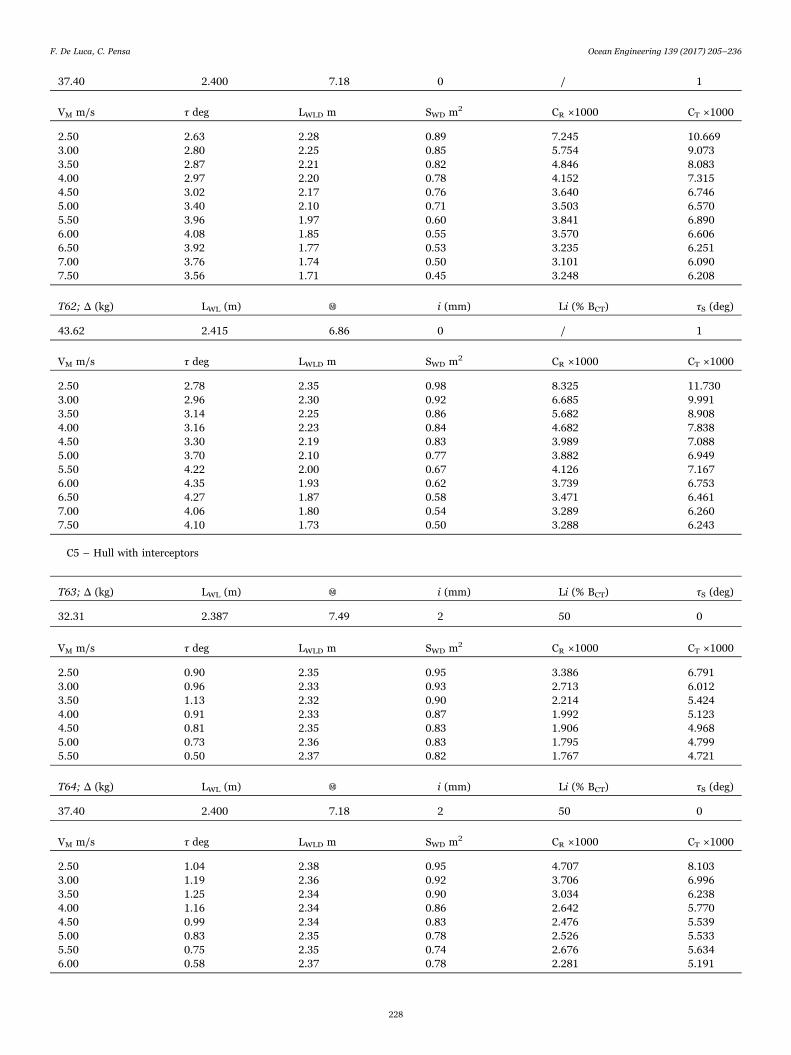
37.40 2.400 7.18 0 / 1
VM m/s τ deg LWLD m SWD m2 CR ×1000 CT ×1000
2.50 2.63 2.28 0.89 7.245 10.6693.00 2.80 2.25 0.85 5.754 9.0733.50 2.87 2.21 0.82 4.846 8.0834.00 2.97 2.20 0.78 4.152 7.3154.50 3.02 2.17 0.76 3.640 6.7465.00 3.40 2.10 0.71 3.503 6.5705.50 3.96 1.97 0.60 3.841 6.8906.00 4.08 1.85 0.55 3.570 6.6066.50 3.92 1.77 0.53 3.235 6.2517.00 3.76 1.74 0.50 3.101 6.0907.50 3.56 1.71 0.45 3.248 6.208
Τ62; Δ (kg) LWL (m) Ⓜ i (mm) Li (% BCT) τS (deg)
43.62 2.415 6.86 0 / 1
VM m/s τ deg LWLD m SWD m2 CR ×1000 CT ×1000
2.50 2.78 2.35 0.98 8.325 11.7303.00 2.96 2.30 0.92 6.685 9.9913.50 3.14 2.25 0.86 5.682 8.9084.00 3.16 2.23 0.84 4.682 7.8384.50 3.30 2.19 0.83 3.989 7.0885.00 3.70 2.10 0.77 3.882 6.9495.50 4.22 2.00 0.67 4.126 7.1676.00 4.35 1.93 0.62 3.739 6.7536.50 4.27 1.87 0.58 3.471 6.4617.00 4.06 1.80 0.54 3.289 6.2607.50 4.10 1.73 0.50 3.288 6.243
C5 – Hull with interceptors
Τ63; Δ (kg) LWL (m) Ⓜ i (mm) Li (% BCT) τS (deg)
32.31 2.387 7.49 2 50 0
VM m/s τ deg LWLD m SWD m2 CR ×1000 CT ×1000
2.50 0.90 2.35 0.95 3.386 6.7913.00 0.96 2.33 0.93 2.713 6.0123.50 1.13 2.32 0.90 2.214 5.4244.00 0.91 2.33 0.87 1.992 5.1234.50 0.81 2.35 0.83 1.906 4.9685.00 0.73 2.36 0.83 1.795 4.7995.50 0.50 2.37 0.82 1.767 4.721
Τ64; Δ (kg) LWL (m) Ⓜ i (mm) Li (% BCT) τS (deg)
37.40 2.400 7.18 2 50 0
VM m/s τ deg LWLD m SWD m2 CR ×1000 CT ×1000
2.50 1.04 2.38 0.95 4.707 8.1033.00 1.19 2.36 0.92 3.706 6.9963.50 1.25 2.34 0.90 3.034 6.2384.00 1.16 2.34 0.86 2.642 5.7704.50 0.99 2.34 0.83 2.476 5.5395.00 0.83 2.35 0.78 2.526 5.5335.50 0.75 2.35 0.74 2.676 5.6346.00 0.58 2.37 0.78 2.281 5.191
F. De Luca, C. Pensa Ocean Engineering 139 (2017) 205–236
228
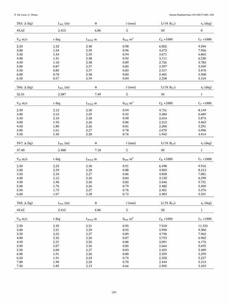
Τ65; Δ (kg) LWL (m) Ⓜ i (mm) Li (% BCT) τS (deg)
43.62 2.415 6.86 2 50 0
VM m/s τ deg LWLD m SWD m2 CR ×1000 CT ×1000
2.50 1.32 2.40 0.98 6.002 9.3943.00 1.54 2.39 0.96 4.673 7.9563.50 1.43 2.39 0.94 3.671 6.8654.00 1.31 2.38 0.92 3.111 6.2304.50 1.10 2.38 0.89 2.726 5.7835.00 0.87 2.37 0.85 2.597 5.5995.50 0.85 2.37 0.83 2.517 5.4706.00 0.70 2.38 0.83 2.401 5.3086.50 0.57 2.39 0.84 2.258 5.124
Τ66; Δ (kg) LWL (m) Ⓜ i (mm) Li (% BCT) τS (deg)
32.31 2.387 7.49 2 50 1
VM m/s τ deg LWLD m SWD m2 CR ×1000 CT ×1000
2.50 2.12 2.30 0.94 4.731 8.1493.00 2.12 2.29 0.92 3.380 6.6893.50 2.10 2.28 0.90 2.654 5.8744.00 1.93 2.26 0.86 2.315 5.4634.50 1.80 2.26 0.81 2.206 5.2915.00 1.61 2.27 0.78 2.070 5.0965.50 1.50 2.28 0.76 1.942 4.914
Τ67; Δ (kg) LWL (m) Ⓜ i (mm) Li (% BCT) τS (deg)
37.40 2.400 7.18 2 50 1
VM m/s τ deg LWLD m SWD m2 CR ×1000 CT ×1000
2.50 2.25 2.30 0.91 6.498 9.9163.00 2.29 2.28 0.88 4.903 8.2133.50 2.34 2.27 0.86 3.858 7.0814.00 2.12 2.26 0.84 3.150 6.2994.50 1.96 2.26 0.82 2.646 5.7315.00 1.76 2.26 0.79 2.482 5.5095.50 1.73 2.27 0.76 2.401 5.3766.00 1.67 2.28 0.72 2.403 5.331
Τ68; Δ (kg) LWL (m) Ⓜ i (mm) Li (% BCT) τS (deg)
43.62 2.415 6.86 2 50 1
VM m/s τ deg LWLD m SWD m2 CR ×1000 CT ×1000
2.50 2.45 2.31 0.95 7.918 11.3333.00 2.51 2.29 0.92 5.990 9.3003.50 2.53 2.27 0.89 4.740 7.9624.00 2.35 2.26 0.87 3.753 6.9024.50 2.21 2.26 0.86 3.091 6.1765.00 2.07 2.26 0.85 2.664 5.6925.50 2.00 2.27 0.83 2.433 5.4096.00 1.91 2.26 0.80 2.359 5.2936.50 1.91 2.24 0.75 2.358 5.2577.00 1.90 2.20 0.70 2.444 5.3147.50 1.85 2.15 0.66 2.505 5.353
F. De Luca, C. Pensa Ocean Engineering 139 (2017) 205–236
229
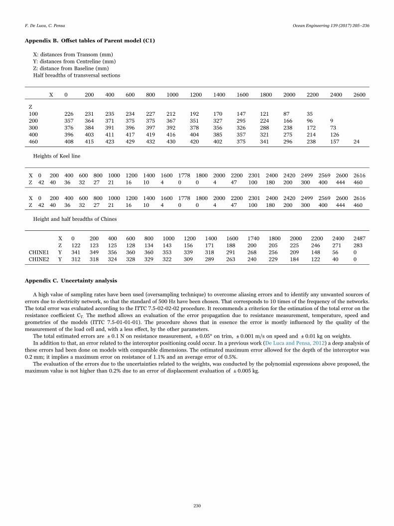
Appendix B. Offset tables of Parent model (C1)
X: distances from Transom (mm)Y: distances from Centreline (mm)Z: distance from Baseline (mm)Half breadths of transversal sections
X 0 200 400 600 800 1000 1200 1400 1600 1800 2000 2200 2400 2600
Z100 226 231 235 234 227 212 192 170 147 121 87 35200 357 364 371 375 375 367 351 327 295 224 166 96 9300 376 384 391 396 397 392 378 356 326 288 238 172 73400 396 403 411 417 419 416 404 385 357 321 275 214 126460 408 415 423 429 432 430 420 402 375 341 296 238 157 24
Heights of Keel line
X 0 200 400 600 800 1000 1200 1400 1600 1778 1800 2000 2200 2301 2400 2420 2499 2569 2600 2616Z 42 40 36 32 27 21 16 10 4 0 0 4 47 100 180 200 300 400 444 460
X 0 200 400 600 800 1000 1200 1400 1600 1778 1800 2000 2200 2301 2400 2420 2499 2569 2600 2616Z 42 40 36 32 27 21 16 10 4 0 0 4 47 100 180 200 300 400 444 460
Height and half breadths of Chines
X 0 200 400 600 800 1000 1200 1400 1600 1740 1800 2000 2200 2400 2487Z 122 123 125 128 134 143 156 171 188 200 205 225 246 271 283
CHINE1 Y 341 349 356 360 360 353 339 318 291 268 256 209 148 56 0CHINE2 Y 312 318 324 328 329 322 309 289 263 240 229 184 122 40 0
Appendix C. Uncertainty analysis
A high value of sampling rates have been used (oversampling technique) to overcome aliasing errors and to identify any unwanted sources oferrors due to electricity network, so that the standard of 500 Hz have been chosen. That corresponds to 10 times of the frequency of the networks.The total error was evaluated according to the ITTC 7.5-02-02-02 procedure. It recommends a criterion for the estimation of the total error on theresistance coefficient CT. The method allows an evaluation of the error propagation due to resistance measurement, temperature, speed andgeometries of the models (ITTC 7.5-01-01-01). The procedure shows that in essence the error is mostly influenced by the quality of themeasurement of the load cell and, with a less effect, by the other parameters.
The total estimated errors are ± 0.1 N on resistance measurement, ± 0.05° on trim, ± 0.001 m/s on speed and ± 0.01 kg on weights.In addition to that, an error related to the interceptor positioning could occur. In a previous work (De Luca and Pensa, 2012) a deep analysis of
these errors had been done on models with comparable dimensions. The estimated maximum error allowed for the depth of the interceptor was0.2 mm; it implies a maximum error on resistance of 1.1% and an average error of 0.5%.
The evaluation of the errors due to the uncertainties related to the weights, was conducted by the polynomial expressions above proposed, themaximum value is not higher than 0.2% due to an error of displacement evaluation of ± 0.005 kg.
F. De Luca, C. Pensa Ocean Engineering 139 (2017) 205–236
230
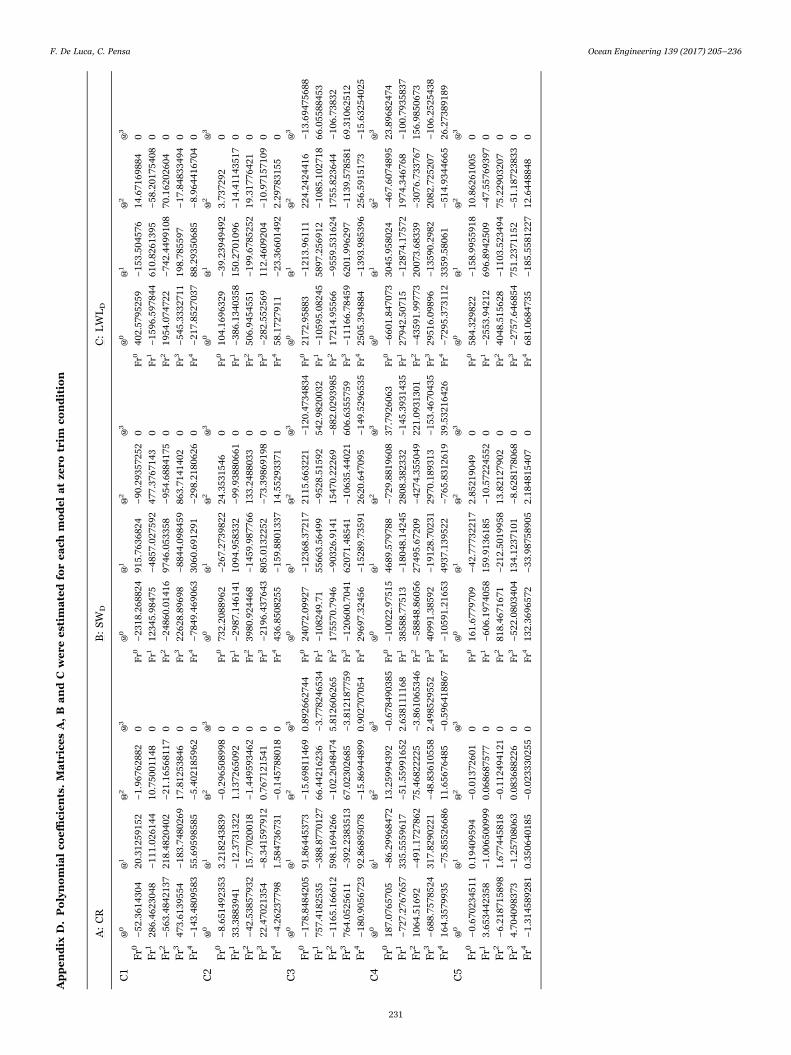
Appendix
D.Polynom
ialco
effi
cients.M
atricesA,B
andC
were
estim
atedfo
reach
modelatze
rotrim
condition
A:CR
B:SW
DC:LWLD
C1
Ⓜ0
Ⓜ1
Ⓜ2
Ⓜ3
Ⓜ0
Ⓜ1
Ⓜ2
Ⓜ3
Ⓜ0
Ⓜ1
Ⓜ2
Ⓜ3
Fr0
−52
.361
4304
20.312
5915
2−1.96
7628
820
Fr0
−23
18.268
824
915.76
3682
4−90
.293
5725
20
Fr0
402.57
9525
9−15
3.50
4576
14.671
6988
40
Fr1
286.46
2304
8−11
1.02
6144
10.750
0114
80
Fr1
1234
5.98
475
−48
57.027
592
477.37
6714
30
Fr1
−15
96.597
844
610.82
6139
5−58
.201
7540
80
Fr2
−56
3.48
4213
721
8.48
2040
2−21
.165
6811
70
Fr2
−24
860.01
416
9746
.053
358
−95
4.68
8417
50
Fr2
1954
.074
722
−74
2.44
9910
870
.162
0260
40
Fr3
473.61
3955
4−18
3.74
8026
917
.812
5384
60
Fr3
2262
8.89
698
−88
44.098
459
863.71
4140
20
Fr3
−54
5.33
3271
119
8.78
5597
−17
.848
3349
40
Fr4
−14
3.48
0958
355
.695
9858
5−5.40
2185
962
0Fr4
−78
49.469
063
3060
.691
291
−29
8.21
8062
60
Fr4
−21
7.85
2703
788
.293
5068
5−8.96
4416
704
0
C2
Ⓜ0
Ⓜ1
Ⓜ2
Ⓜ3
Ⓜ0
Ⓜ1
Ⓜ2
Ⓜ3
Ⓜ0
Ⓜ1
Ⓜ2
Ⓜ3
Fr0
−8.65
1492
353
3.21
8243
839
−0.29
6508
998
0Fr0
732.20
8896
2−26
7.27
3982
224
.353
1546
0Fr0
104.16
9632
9−39
.239
4949
23.73
7292
0
Fr1
33.388
3941
−12
.373
1322
1.13
7265
092
0Fr1
−29
87.146
141
1094
.958
332
−99
.938
8066
10
Fr1
−38
6.13
4035
815
0.27
0109
6−14
.411
4351
70
Fr2
−42
.538
5793
215
.770
2001
8−1.44
9593
462
0Fr2
3980
.924
468
−14
59.987
766
133.24
8803
30
Fr2
506.94
5455
1−19
9.67
8525
219
.317
7642
10
Fr3
22.470
2135
4−8.34
1597
912
0.76
7121
541
0Fr3
−21
96.437
643
805.01
3225
2−73
.398
6919
80
Fr3
−28
2.55
2569
112.46
0920
4−10
.971
5710
90
Fr4
−4.26
2377
981.58
4736
731
−0.14
5788
018
0Fr4
436.85
0825
5−15
9.88
0133
714
.552
9337
10
Fr4
58.172
7911
−23
.366
0149
22.29
7831
550
C3
Ⓜ0
Ⓜ1
Ⓜ2
Ⓜ3
Ⓜ0
Ⓜ1
Ⓜ2
Ⓜ3
Ⓜ0
Ⓜ1
Ⓜ2
Ⓜ3
Fr0
−17
8.84
8420
591
.864
4537
3−15
.698
1146
90.89
2662
744
Fr0
2407
2.09
927
−12
368.37
217
2115
.663
221
−12
0.47
3483
4Fr0
2172
.958
83−12
13.961
1122
4.24
2441
6−13
.694
7568
8
Fr1
757.41
8253
5−38
8.87
7012
766
.442
1623
6−3.77
8246
534
Fr1
−10
8249
.71
5566
3.56
499
−95
28.515
9254
2.98
2003
2Fr1
−10
595.08
245
5897
.256
912
−10
85.102
718
66.055
8845
3
Fr2
−11
65.166
612
598.16
9426
6−10
2.20
4847
45.81
2606
265
Fr2
1755
70.794
6−90
326.91
4115
470.22
269
−88
2.02
9398
5Fr2
1721
4.95
566
−95
59.531
624
1755
.823
644
−10
6.73
832
Fr3
764.05
2561
1−39
2.23
8351
367
.023
0268
5−3.81
2187
759
Fr3
−12
0600
.704
162
071.48
541
−10
635.44
021
606.63
5575
9Fr3
−11
166.78
459
6201
.996
297
−11
39.578
581
69.310
6251
2
Fr4
−18
0.90
5672
392
.868
9507
8−15
.869
4489
90.90
2707
054
Fr4
2969
7.32
456
−15
289.73
591
2620
.647
095
−14
9.52
9653
5Fr4
2505
.394
884
−13
93.985
396
256.59
1517
3−15
.632
5402
5
C4
Ⓜ0
Ⓜ1
Ⓜ2
Ⓜ3
Ⓜ0
Ⓜ1
Ⓜ2
Ⓜ3
Ⓜ0
Ⓜ1
Ⓜ2
Ⓜ3
Fr0
187.07
6570
5−86
.299
6847
213
.259
9439
2−0.67
8490
385
Fr0
−10
022.97
515
4689
.579
788
−72
9.88
1960
837
.792
6063
Fr0
−66
01.847
073
3045
.958
024
−46
7.60
7489
523
.896
8247
4
Fr1
−72
7.27
6765
733
5.55
5961
7−51
.559
9165
22.63
8111
168
Fr1
3858
8.77
513
−18
048.14
245
2808
.382
332
−14
5.39
3143
5Fr1
2794
2.50
715
−12
874.17
572
1974
.346
768
−10
0.79
3583
7
Fr2
1064
.516
92−49
1.17
2786
275
.468
2222
5−3.86
1065
346
Fr2
−58
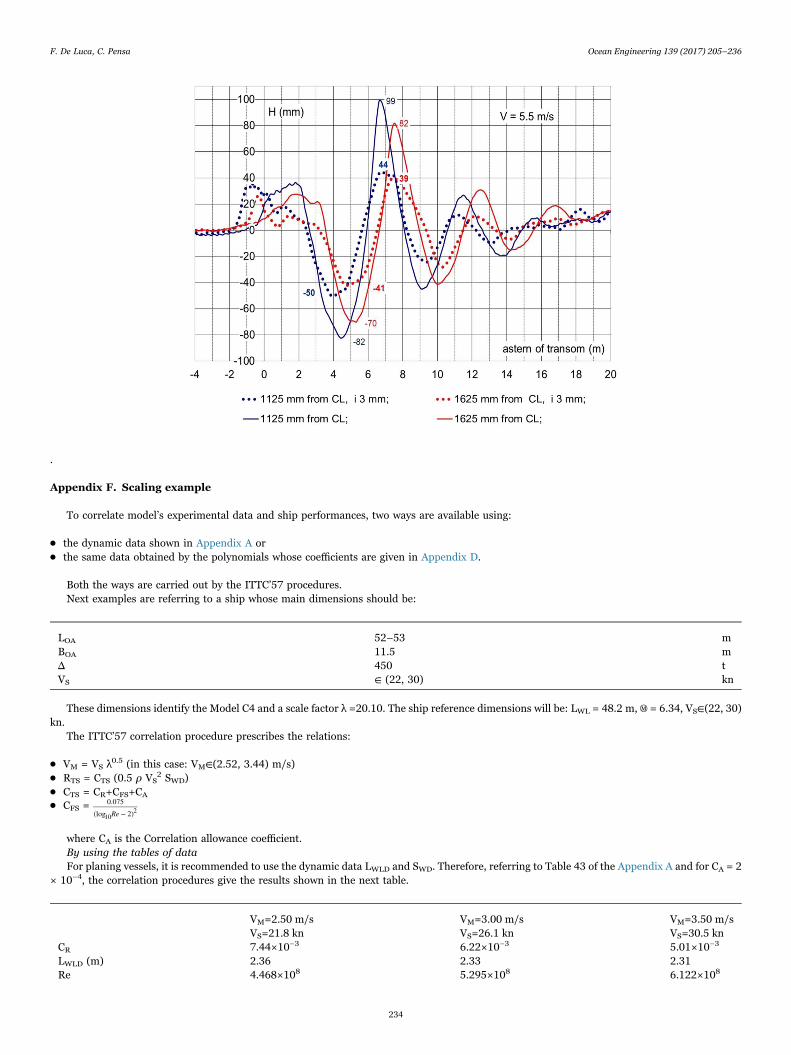
848.86
056
2749
5.67
209
−42
74.355
049
221.09
3130
1Fr2
−43
591.99
773
2007
3.68
339
−30
76.733
767
156.98
5067
3
Fr3
−68
8.75
7852
431
7.82
9022
1−48
.836
1055
82.49
8529
552
Fr3
4099
1.38
592
−19
128.70
231
2970
.189
313
−15
3.46
7043
5Fr3
2951
6.09
896
−13
590.29
8220
82.725
207
−10
6.25
2543
8
Fr4
164.35
7993
5−75
.855
2668
611
.656
7648
5−0.59
6418
867
Fr4
−10
591.21
653
4937
.139
522
−76
5.83
1261
939
.532
1642
6Fr4
−72
95.373
112
3359
.580
61−51
4.93
4466
526
.273
8918
9
C5
Ⓜ0
Ⓜ1
Ⓜ2
Ⓜ3
Ⓜ0
Ⓜ1
Ⓜ2
Ⓜ3
Ⓜ0
Ⓜ1
Ⓜ2
Ⓜ3
Fr0
−0.67
0234
511
0.19
4095
94−0.01
3726
010
Fr0
161.67
7970
9−42
.777
3221
72.85
2190
490
Fr0
584.32
9822
−15
8.99
5591
810
.862
6100
50
Fr1
3.65
3442
358
−1.00
6500
999
0.06
8687
577
0Fr1
−60
6.19
7405
815
9.91
3618
5−10
.572
2455
20
Fr1
−25
53.942
1269
6.89
4250
9−47
.557
6939
70
Fr2
−6.21
8715
898
1.67
7445
818
−0.11
2494
121
0Fr2
818.46
7167
1−21
2.50
1995
813
.821
2790
20
Fr2
4048
.515
628
−11
03.523
494
75.229
0320
70
Fr3
4.70
4098
373
−1.25
7080
630.08
3688
226
0Fr3
−52
2.08
0340
413
4.12
3710
1−8.62
8178
068
0Fr3
−27
57.646
854
751.23
7115
2−51
.187
2383
30
Fr4
−1.31
4589
281
0.35
0640
185
−0.02
3330
255
0Fr4
132.36
9657
2−33
.987
5890
52.18
4815
407
0Fr4
681.06
8473
5−18
5.55
8122
712
.644
8848
0
F. De Luca, C. Pensa Ocean Engineering 139 (2017) 205–236
231
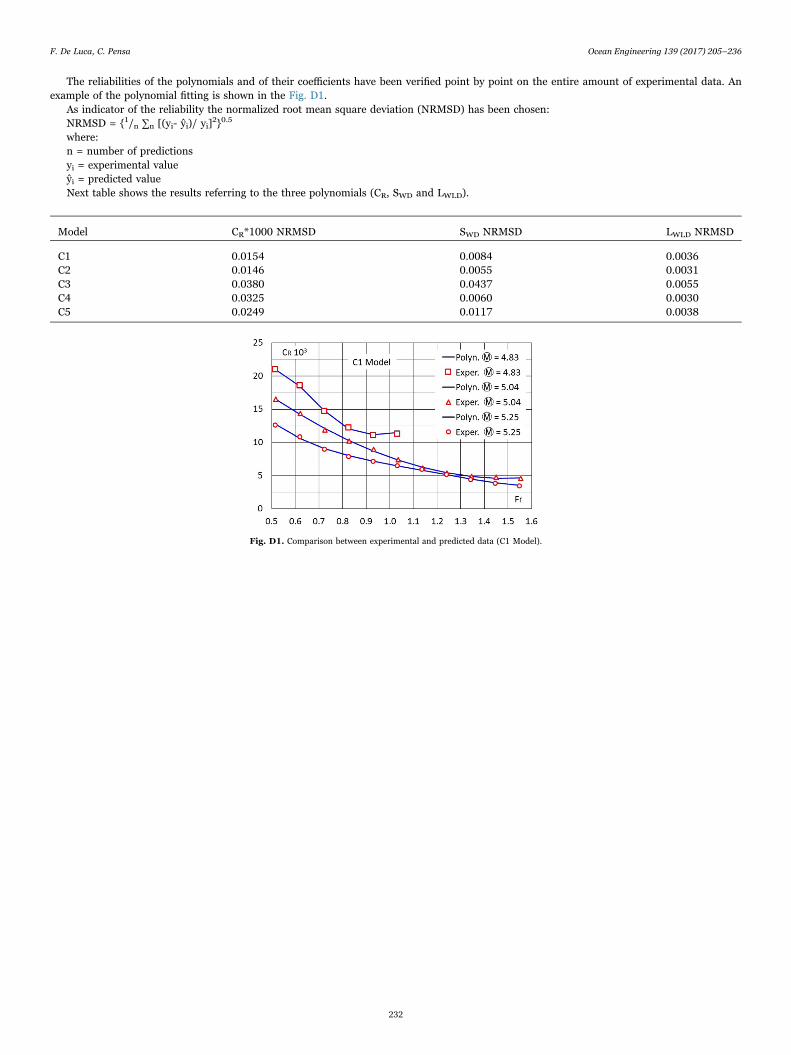
The reliabilities of the polynomials and of their coefficients have been verified point by point on the entire amount of experimental data. Anexample of the polynomial fitting is shown in the Fig. D1.
As indicator of the reliability the normalized root mean square deviation (NRMSD) has been chosen:NRMSD = {1/n ∑n [(yi- ŷi)/ yi]
2}0.5
where:n = number of predictionsyi = experimental valueŷi = predicted valueNext table shows the results referring to the three polynomials (CR, SWD and LWLD).
Model CR*1000 NRMSD SWD NRMSD LWLD NRMSD
C1 0.0154 0.0084 0.0036C2 0.0146 0.0055 0.0031C3 0.0380 0.0437 0.0055C4 0.0325 0.0060 0.0030C5 0.0249 0.0117 0.0038
Fig. D1. Comparison between experimental and predicted data (C1 Model).
F. De Luca, C. Pensa Ocean Engineering 139 (2017) 205–236
232
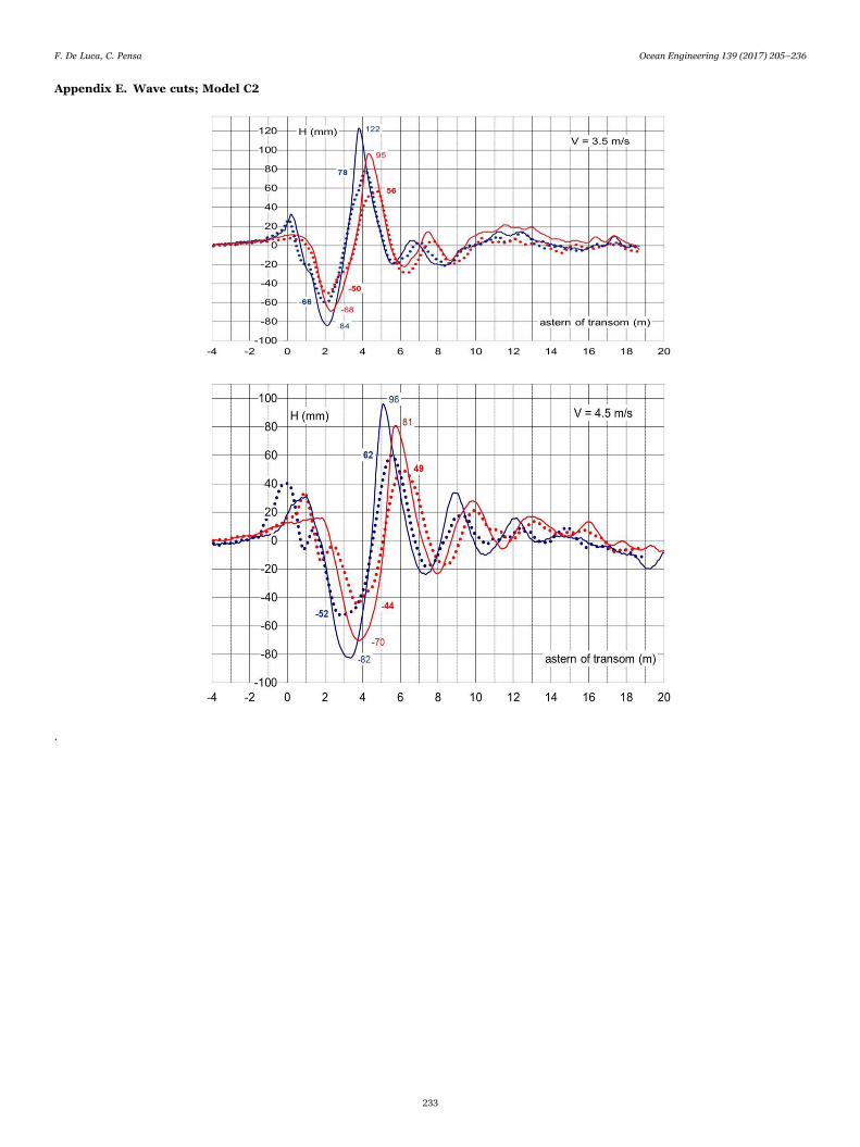
Appendix E. Wave cuts; Model C2
.
F. De Luca, C. Pensa Ocean Engineering 139 (2017) 205–236
233
.
Appendix F. Scaling example
To correlate model’s experimental data and ship performances, two ways are available using:
• the dynamic data shown in Appendix A or
• the same data obtained by the polynomials whose coefficients are given in Appendix D.
Both the ways are carried out by the ITTC’57 procedures.Next examples are referring to a ship whose main dimensions should be:
LOA 52–53 mBOA 11.5 mΔ 450 tVS ∈ (22, 30) kn
These dimensions identify the Model C4 and a scale factor λ =20.10. The ship reference dimensions will be: LWL = 48.2 m, Ⓜ = 6.34, VS∈(22, 30)kn.
The ITTC’57 correlation procedure prescribes the relations:
• VM = VS λ0.5 (in this case: VM∈(2.52, 3.44) m/s)
• RTS = CTS (0.5 ρ VS2 SWD)
• CTS = CR+CFS+CA
• CFS =Re
0.075(log − 2)10
2
where CA is the Correlation allowance coefficient.By using the tables of dataFor planing vessels, it is recommended to use the dynamic data LWLD and SWD. Therefore, referring to Table 43 of the Appendix A and for CA = 2
× 10−4, the correlation procedures give the results shown in the next table.
VM=2.50 m/s VM=3.00 m/s VM=3.50 m/sVS=21.8 kn VS=26.1 kn VS=30.5 kn
CR 7.44×10⁻³ 6.22×10⁻³ 5.01×10⁻³
LWLD (m) 2.36 2.33 2.31Re 4.468×10⁸ 5.295×10⁸ 6.122×10⁸
F. De Luca, C. Pensa Ocean Engineering 139 (2017) 205–236
234
CFS 1.696×10⁻³ 1.659×10⁻³ 1.628×10⁻³
CTS 9.34×10⁻³ 7.90×10⁻³ 6.66×10⁻³
SWD (m2) 1.17 1.14 1.1RTS (kN) 283.2 344.6 381.6
Obviously, for models with interceptors, the calculation procedure is the same. Nevertheless it has been highlighted that there is a significantscale effect in the correlation of the interceptor work in ship scale. In particular, in model scale the effectiveness of the interceptor (as trim correctorand as high lift device) is underrated. This underestimate is due to the non-proportional boundary layer and is growing with the scale factor. Thistheme is described in detail in (De Luca and Pensa, 2012).
By using the polynomialsIt is possible to perform the same example using the polynomial expressions. The vectors Ⓜ and Fr should be calculate for the speeds of interest.ⓂT = {1, Ⓜ, Ⓜ 2, Ⓜ 3} = {1, 6.341, 40.208, 254.961}
VS = 21.8 kn:FrT = {1, Fr, Fr2, Fr3, Fr4} = {1, 0.515, 0.265, 0.137, 0.070}VS = 30.5 kn:FrT = {1, Fr, Fr2, Fr3, Fr4} = {1, 0.721, 0.520, 0.375, 0.270}By the next expressions, it is possible to calculate CR, SWD and LWLD.CR = (Fr)T·A Ⓜ
SWD = (Fr)T·B Ⓜ
LWLD = (Fr)T·C Ⓜ
To be clear, the calculation of the CR at VS = 21.8 kn is shown.⎛
⎝
⎜⎜⎜⎜⎜
⎞
⎠
⎟⎟⎟⎟⎟
⎛
⎝
⎜⎜⎜
⎞
⎠
⎟⎟⎟V T1 : CR = (Fr) ·AⓂ = (1, 0. 515, 0. 265, 0. 137, 0. 070)·
187.0765705, − 86.2996847, 13.25994392, − 0.6784904−727.276765, 335.5559617, − 51.55991652, 2.63811121064.51692, − 491.172786, 75.46822225, − 3.8610653−688.757852, 317.8290221, − 48.83610558, 2.4985296164.3579935, − 75.8552669, 11.65676485, − 0.5964189
16. 341
40. 208254. 961
= 0. 0075214
The results are:
VS CR SWD LWLD
kn (m2) (m)
21.8 0.0075214 1.17 2.3630.5 0.0050002 1.10 2.32
Now it is possible to repeat the same ITTC’57 procedures above shown and taking ΔCF=2·10 −4 , it is possible to articulate the resistance by asingle expression
RTS = {[(Fr)T A·Ⓜ]+{0.075/{Log10{{Vs [(Fr)T·C Ⓜ] λ)/νs}−2}2}+ΔCF}1/2ρ[(Fr)T·B Ⓜ] λ2 Vs2
VS (kn) ReS CFS CTS RTS (kN)
21.8 4.465E+08 0.0016961 0.009418 286.230.5 6.135E+08 0.0016278 0.006828 382.5
By the following expressions it is possible to evaluate the sensitivity of the resistance to the displacement.∂CR/∂Ⓜ = (Fr)T·A Ⓜi;∂SWD/∂Ⓜ = (Fr)T·B Ⓜi;∂LWLD/∂Ⓜ = (Fr)T·C Ⓜi;Ⓜi
T = {0, 1, 2Ⓜ, 3Ⓜ2, 4Ⓜ3, 5Ⓜ4}for Ⓜ = 6.34Ⓜi
T = {0, 1, 12.682, 120.625}whereas an increase of the displacement of 1.0% leads to reducing the Ⓜ of 0.02, the above mentioned expressions give the following derivatives.
VS (kn) ∂CR/∂Ⓜ ∂SWD/∂Ⓜ ∂LWLD/∂Ⓜ
21.8 −0.002524 −0.713 −0.1530.5 −0.003053 −0.187 −0.04
The next expressions give the variations of CR, SWD and LWLD:δCR = - δⓂ·∂CR /∂Ⓜ.δSWD = - δⓂ·∂SWD /∂Ⓜ.δLWLD = - δⓂ·∂LWLD /∂Ⓜ.
VS (kn) δCR* δSWD*(m2) δLWLD*(m)
21.8 0.000051 0.0143 0.003130.5 0.000061 0.0037 0.0008
F. De Luca, C. Pensa Ocean Engineering 139 (2017) 205–236
235
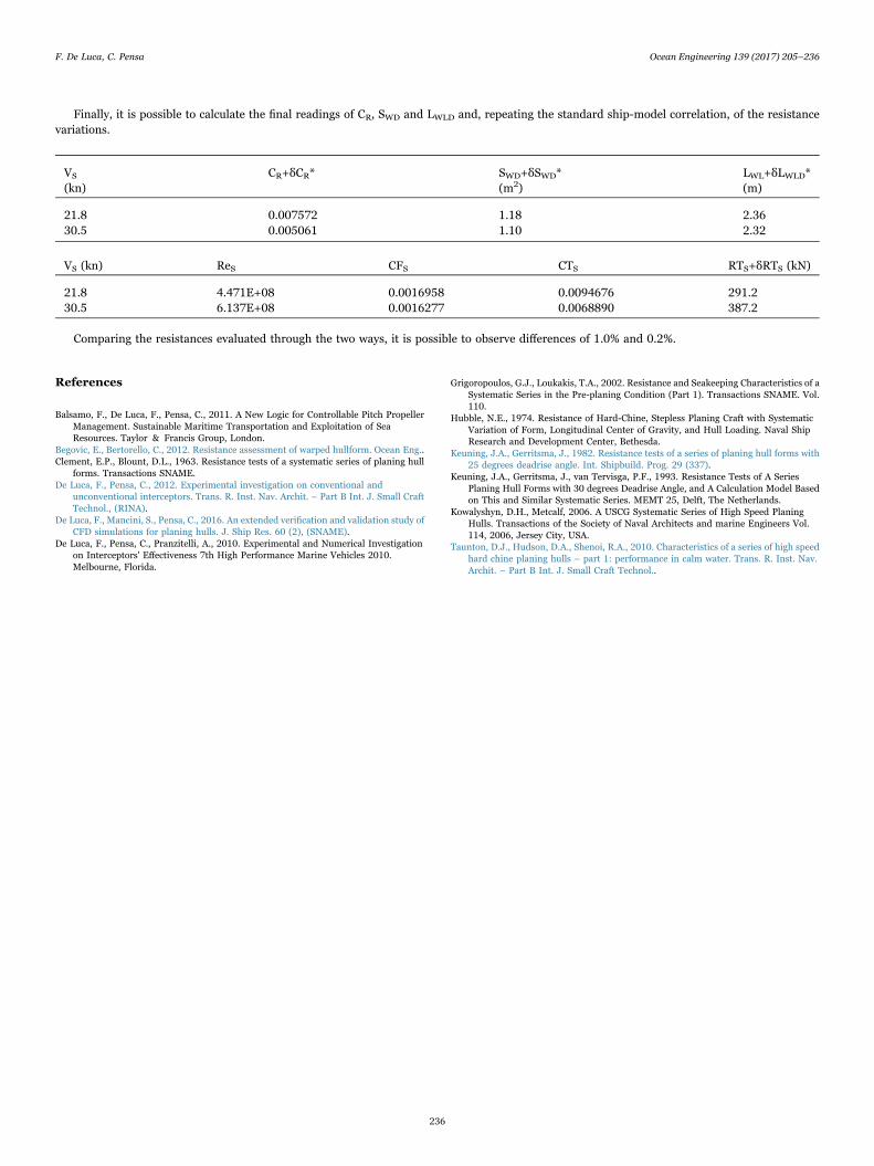
Finally, it is possible to calculate the final readings of CR, SWD and LWLD and, repeating the standard ship-model correlation, of the resistancevariations.
VS CR+δCR* SWD+δSWD* LWL+δLWLD*(kn) (m2) (m)
21.8 0.007572 1.18 2.3630.5 0.005061 1.10 2.32
VS (kn) ReS CFS CTS RTS+δRTS (kN)
21.8 4.471E+08 0.0016958 0.0094676 291.230.5 6.137E+08 0.0016277 0.0068890 387.2
Comparing the resistances evaluated through the two ways, it is possible to observe differences of 1.0% and 0.2%.
References
Balsamo, F., De Luca, F., Pensa, C., 2011. A New Logic for Controllable Pitch PropellerManagement. Sustainable Maritime Transportation and Exploitation of SeaResources. Taylor & Francis Group, London.
Begovic, E., Bertorello, C., 2012. Resistance assessment of warped hullform. Ocean Eng..Clement, E.P., Blount, D.L., 1963. Resistance tests of a systematic series of planing hull
forms. Transactions SNAME.De Luca, F., Pensa, C., 2012. Experimental investigation on conventional and
unconventional interceptors. Trans. R. Inst. Nav. Archit. – Part B Int. J. Small CraftTechnol., (RINA).
De Luca, F., Mancini, S., Pensa, C., 2016. An extended verification and validation study ofCFD simulations for planing hulls. J. Ship Res. 60 (2), (SNAME).
De Luca, F., Pensa, C., Pranzitelli, A., 2010. Experimental and Numerical Investigationon Interceptors' Effectiveness 7th High Performance Marine Vehicles 2010.Melbourne, Florida.
Grigoropoulos, G.J., Loukakis, T.A., 2002. Resistance and Seakeeping Characteristics of aSystematic Series in the Pre-planing Condition (Part 1). Transactions SNAME. Vol.110.
Hubble, N.E., 1974. Resistance of Hard-Chine, Stepless Planing Craft with SystematicVariation of Form, Longitudinal Center of Gravity, and Hull Loading. Naval ShipResearch and Development Center, Bethesda.
Keuning, J.A., Gerritsma, J., 1982. Resistance tests of a series of planing hull forms with25 degrees deadrise angle. Int. Shipbuild. Prog. 29 (337).
Keuning, J.A., Gerritsma, J., van Tervisga, P.F., 1993. Resistance Tests of A SeriesPlaning Hull Forms with 30 degrees Deadrise Angle, and A Calculation Model Basedon This and Similar Systematic Series. MEMT 25, Delft, The Netherlands.
Kowalyshyn, D.H., Metcalf, 2006. A USCG Systematic Series of High Speed PlaningHulls. Transactions of the Society of Naval Architects and marine Engineers Vol.114, 2006, Jersey City, USA.
Taunton, D.J., Hudson, D.A., Shenoi, R.A., 2010. Characteristics of a series of high speedhard chine planing hulls – part 1: performance in calm water. Trans. R. Inst. Nav.Archit. – Part B Int. J. Small Craft Technol..
F. De Luca, C. Pensa Ocean Engineering 139 (2017) 205–236
236