The Myth of the Discounted Cash Flow #2 - Actuaries

Tom Mullin November 2003

The Myth of the Discounted Cash Flow

(How Uncertainty Affects Liabilities)

by

Tom Mullin

[email protected]

The Myth of the Discounted Cash Flow Page 2


Table of Contents

1. Précis .......................................................................................................................3

2. Introduction............................................................................................................4

3. Adding Uncertainty to Net Present Value ................................................................5

3.1 The Chaotic Problem of Equities .........................................................................5

3.2 Example – Australian Equities ............................................................................8

4. Computational Description (largely graphical)......................................................10

5. An Actual Example Using Real Data.....................................................................12

6. Comparison of the Probability Distribution of Liabilities to Standard Practises ...16

6.1 Impact of Increasing Payment Forecast Uncertainty.........................................16

6.2 Increasing Uncertainty at Extreme Values ........................................................18

6.3 Combining Multiple Injury Years and/or Product Lines ...................................19

7. Conclusions and Future Research to be Completed...............................................20

7.1 Conclusions .......................................................................................................20

7.2 Further Research to be Undertaken..................................................................20

7.3 Caveat ...............................................................................................................21



1. Précis

This paper is about the application of uncertainty to the calculation of discounted liabilities.

Formula non-linearities plus cashflow forecasting uncertainties, combined with non-parametric and non-linear investment return distributions and uncertainty of future inflationrates are combined to create a probability distribution of discounted liabilities.

It is demonstrated that where equity investments are used, the chaotic nature of investmentreturns renders standard techniques (such as a single pass Markov chain) invalid. It is alsodemonstrated that many of the approaches normally used in dynamic financial analysis arealso incomplete.

The only apparently valid approach utilises simulation techniques to calculate the probabilitydistributions of discounted liabilities, essentially using multiple Monte Carlo Markov chains.

The result of an actual calculation is presented using actual investment and CPI rates plustheir uncertainty, combined with combined cashflow forecast uncertainty. Risk levels(probability of failure) are calculated and compared with current standard techniques.

It will be shown that the uncertainties and non-linearities combine to give higher probabilitiesof failure (defined as insufficient premium to meet liabilities) than is commonly understood,particularly for long tailed insurance classes.

The ‘contamination’ effect of equities is discussed as well as the need to design models tosuite the specific circumstances that actually exist. Model design will depend on theinvestment portfolio profile, the cash inflow/outflow timings and the uncertainties in expectedcash payments.

Some ideas of some possible investment and cashflow optimisation techniques are alsodiscussed, indicating how reductions in liability uncertainty can be achieved.

The methodology demonstrated is mathematically straightforward but computationallydemanding, but is within the reach of current, high-end workstations.

This paper demonstrates that it is practically possible to calculate solutions to the problem ofliability uncertainty, even where there are chaotic investment returns.

.The applicability of this methodology applies to all general and life insurance as well as

supperannuation, project finance and investment analysis.



2. Introduction

Discounted liability is the cornerstone of pricing in insurance.

Stated simply, what amount of money do I need to collect today (premium) to meet mypayment obligation in the future. The time honoured method is to forecast the expectedcashflow (by some method), then calculate the present value, taking into account expectedinvestment income and the effects of inflation (where appropriate). The formula is:

( )( )∑

− ++n

ii

i

iii

inv

CF

1 1

)inf1

Where Cfi is the payment expected to be made at time i, and inf and inv are theexpected inflation and investment earning rates at time i.

Typically, though not always, only single investment earning and inflation rates are applied toall years.

This equation (dating back to at least the 1700s) is based on the following assumptions:

(1) The cashflow will actually happen at time i.(2) The investment earning rate will actually be inv at time i.(3) The inflation rate will actually be inf at time i.

However, the value calculated is only valid if the cashflows are accurate, the investmentearning rates actually achieved and inflation is what is predicted. The formula was originallydeveloped to calculate the expected returns on loans and calculate annuities. Long used in lifeinsurance, very stable data (life expectancy) was combined with conservative investments(rents and later government bonds).

Currently it is typical for an organisation to calculate the money required using a nominal(safe) earning rate and an assumption that the inflation rate is some (on average) amountlower than the nominal investment rate. Loadings will be added to create a prudential margin.Often organisations will normally invest their money in higher earning investments, oftenwith a large component in equities. The assumption is that the higher investment earning rateachieved will exceed the effects of any uncertainty in cashflow and inflation.

Unfortunately these assumptions are unrealistic. Any forecast of future payments is uncertain,inflation exhibits random uncertainty and any investment has an uncertain return (unless theyare Government bonds that are held to maturity).

The problem is how to combine these uncertainties and present a probability distribution oftotal liabilities, making it possible to determine what risks are actually being faced. If this canbe achieved, rational decisions can then be made about what premium levels and investmentportfolio mixes are appropriate.



3. Adding Uncertainty to Net Present Value

There are four sources of uncertainty:

(1) Inflation varies. Even in times of low, stable inflation rates there is an inherentuncertainty in inflation. Where there are trend changes (rising or falling) uncertainty ismagnified.

(2) Forecast cashflow. Every forecast has an inherent uncertainty ε . The distribution of εdepends on the forecasting method and the uncertainty in the originating data.

(3) Investment earning rates. All investments are uncertain, interest rates have significantuncertainty, bond yields vary considerably and equities have been proven to be a chaotic,fractal series. Again any trend changes magnify uncertainty.

(4) The forecast of future cashflows is typically non-linear, declining through time. (Littlesuccess has been made in fitting single continuous functions to long tailed insurancecashflows, the closest being weibull functions). This non-linear sinking fund creates a‘gearing’ effect, small changes in values at the beginning of the sinking fund can havelarge effects on the total cash outcomes. This amplifies the effects of cashflow andearning uncertainty. In simple terms slightly lower returns in the earlier years, when thecash balance is large, would have to be offset by much higher returns in later years, whenthe cash balance is small.

The total uncertainty is the product of all the uncertainties in all possible combinations. Thisuncertainty is multiplied by the non-linearity of the equation (for example; the ratio of a 4%inflation rate and a 7% investment earning rate is 0.97 at year 1 and 0.57 at year 20).

Can all uncertainties be combined and calculated to create a probability distribution ofdiscounted liabilities and hence calculate the risk probabilities of insufficient premium?

3.1 The Chaotic Problem of Equities

It is necessary to digress to examine the issue of equities and why their chaotic, fractal naturerenders standard solutions ineffective.

• Firstly, it has been well established that stock returns are non-Gaussian1. This means thatapproaches based on Brownian random walk models are invalid.

• Secondly there is evidence that there are no ‘short memory’ effects and contradictoryevidence for ‘long memory’ effects. This means that a value in the near future is notdependent on an earlier value and a value in the long term future may or may not bedependent on an earlier value 1&2 .

• Thirdly, stock indices exhibit scale invariance, that is, patterns appear the same onwhatever time scale they are viewed. A minute by minute series will appear similar to ayear by year series.

• Fourthly, large fluctuations can occur in the both short and long terms.• Fifthly, heteroscedasticity is common for values and returns. This means that variances

change through time and these variance changes are in themselves random andunpredictable.

1 See, for example, Brock, W.A., and de Lima, P.J.F. (1995), "Nonlinear Time Series, ComplexityTheory, and Finance", Preprint, Social Systems Research Institute, University of Wisconsin-Madison.

2 I.N. Lobato and N.E. Savin (1998), “Real and Spurious Long Memory Properties of Stock MarketData”, Journal of Business and Economic Statistics.



Current theory suggests that markets are the impact of mass psychological effects of allparticipants, with non-linear feedback mechanisms that self-reinforce independent events andcause irregular behaviour.3

From the point of view of solving current practical problems, these characteristics (andothers) render predictability of stock market returns impossible across any time period.

This contrasts with bond and cash yields, which though they exhibit uncertainty, do not havethe chaotic effects nature of equities. For example, Bonds are moderately correlated (R2 of0.54) to CPI, and exhibit Gaussian properties.

(1) It is common to maintain a mixed portfolio to manage risk, the idea being that aproportion of lower risk investments (e.g. bonds) create a base amount that relatively safe,reducing the overall risk of the total portfolio.

(2) What actually happens is that the more volatile (and chaotic) proportion of theinvestments that is held in equities ‘contaminates’ the total portfolio. Their characteristicsand probability distribution of returns influencing the whole portfolio to a greater andgreater extent as their proportion grows.

(4) This is not the same as the combination of two similar (parametric) distributions, which iswell understood and can easily be calculated. A well behaved distribution combined witha chaotic distribution will produce a chaotic distribution.

(5) This can be demonstrated by the following ‘thought experiment’:

• Take an amount of bonds combined with a smaller amount of equities.• In a given year the bonds deliver a return, well within expected (and narrow)

confidence limits.• In the same year the equities exhibit a large negative fluctuation in returns, well

within the range of such returns made in the past, but well outside the range of returnsin the bond portfolio.

• The total portfolio has now a lower return than expected.• To meet payment demands a sale of investments is required, crystallising the

fluctuation.• The whole portfolio is now in deficit.• With bond returns being predictable within reasonable confidence limits, the only

way the fund can return to balance is if the equities return a correspondingly highreturn, or a long period of above average returns.

What is happening is that the chaotic uncertainty in returns of the smaller number of equitiesis driving the total portfolio return probabilities. In other words:

Chaos Contaminates

Of course if the proportion of equities is very small then the effects will be more muted, as theproportion grows then the distribution of returns will then tend to take on the distribution ofthe equity part. Essentially the variance of the total portfolio will increase, with thedistribution becoming more chaotic like as the proportion increases.

3 “ Chinese Stock Market – Is it Chaos?” [Ref]



What is just as important is that other chaotic characteristics will contaminate the wholeportfolio, with correlations of returns between years dropping and heteroscedasticityincreasing.

Three additional points should be added:

(1) It is not known what proportion of equities is required to have a noticeable effect.Intuitively a very small proportion (say 1%) will be insignificant, but a larger amount(20%, 30%?) will be noticeable. This is a fruitful area for research.

The proportion may be smaller than common sense would expect because of the largefluctuation effect of chaos.

(2) There may be ways to buffer bonds from equity effects, provided the proportion is not toogreat. A cash ‘float’ that is sufficient to cover most probabilities (which can be calculatedby a stochastic EOQ* formula) could be utilised to prevent forced sales, thus avoiding thecrystallisation of losses and hence buying time for the fluctuation to smooth out.

It should be noted that this amount will be related (in a currently unknown way) to theproportion of equities and will probably be much larger than would commonly bethought, though theoretically calculable.

(3) This issue of contamination is of particular relevance to investment in overseas equities,while the jury is still out on whether exchange rates are chaotic and whether they do or donot exhibit ‘long memory’ effects, their returns will be chaotic in nature, combined withfurther exchange rate uncertainty.

* Economic Order Quantity, note that this approach can also be used to determine the cashbalance necessary to avoid bond tranding (and thus potential capital losses) for a purelycash/bond porfolio.



3.2 Example – Australian Equities

It is worthwhile to examine these characteristics to determine whether they apply toAustralian equities. The daily indices of the Australian All ordinaries for the last 20 yearsare:

The annual rates of return by day is:Chart 1

The distribution of annual returns, compared with normal and log-normal distributions are:Chart 2

A u s t r a l i a n A l l O r d i n a r i e s , 3 / 8 / 1 9 8 3 t o 2 9 / 4 / 2 0 0 3 b y D a y

-

5 0 0

1 , 0 0 0

1 , 5 0 0

2 , 0 0 0

2 , 5 0 0

3 , 0 0 0

3 , 5 0 0

4 , 0 0 0

1984

08.0

3

1985

02.0

6

1985

08.0

1

1986

01.2

3

1986

07.2

1

1987

01.1

2

1987

07.0

7

1987

12.2

4

1988

06.2

4

1988

12.1

4

1989

06.1

3

1989

11.3

0

1990

05.3

1

1990

11.2

0

1991

05.2

1

1991

11.0

8

1992

05.0

6

1992

10.2

6

1993

04.2

1

1993

10.1

1

1994

04.0

7

1994

09.2

8

1995

03.2

3

1995

09.1

5

1996

03.1

1

1996

09.0

3

1997

02.2

6

1997

08.2

1

1998

02.1

3

1998

08.0

7

1999

02.0

1

1999

07.2

6

2000

01.1

8

2000

07.1

2

2001

01.0

3

2001

06.2

9

2002

01.0

3

2002

07.0

1

2002

12.2

0

Annual Equity Returns, Daily All Ordinaries Index for last 20 Yearsvs Normal & Log Normal Distributions

0.00%

0.50%

1.00%

1.50%

2.00%

2.50%

3.00%

3.50%

4.00%

4.50%

5.00%

-50.

0%

-45.

0%

-40.

0%

-35.

0%

-30.

0%

-25.

0%

-20.

0%

-15.

0%

-10.

0%

-5.0

%

0.0%

5.0%

10.0

%

15.0

%

20.0

%

25.0

%

30.0

%

35.0

%

40.0

%

45.0

%

50.0

%

55.0

%

60.0

%

65.0

%

70.0

%

75.0

%

80.0

%

85.0

%

90.0

%

95.0

%

100.

0

% Annual Return

Pro

po

rtio

n Stock Returns

Normal DistClipped Normal Dist

Log Nomal Dist



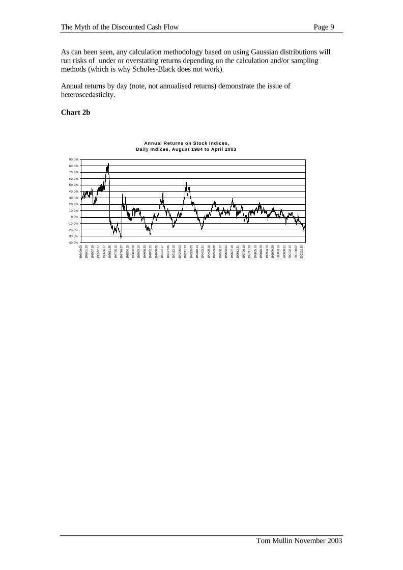
As can been seen, any calculation methodology based on using Gaussian distributions willrun risks of under or overstating returns depending on the calculation and/or samplingmethods (which is why Scholes-Black does not work).

Annual returns by day (note, not annualised returns) demonstrate the issue ofheteroscedasticity.

Chart 2b

Annual Returns on Stock Indices,Daily Indices, August 1984 to April 2003

-40.0%

-30.0%

-20.0%

-10.0%

0.0%

10.0%

20.0%

30.0%

40.0%

50.0%

60.0%

70.0%

80.0%

90.0%

1984

08.0

3

1985

01.2

9

1985

07.1

6

1985

12.2

7

1986

06.1

7

1986

11.2

6

1987

05.1

5

1987

10.2

7

1988

04.1

5

1988

09.2

8

1989

03.1

5

1989

08.3

0

1990

02.1

5

1990

08.0

2

1991

01.1

7

1991

07.0

5

1991

12.1

6

1992

06.0

3

1992

11.1

3

1993

05.0

3

1993

10.1

4

1994

03.3

1

1994

09.1

5

1995

03.0

2

1995

08.1

7

1996

02.0

1

1996

07.1

8

1996

12.3

1

1997

06.1

9

1997

11.2

8

1998

05.1

9

1998

10.2

9

1999

04.1

9

1999

09.2

9

2000

03.1

6

2000

08.3

1

2001

02.1

5

2001

08.0

2

2002

01.3

0



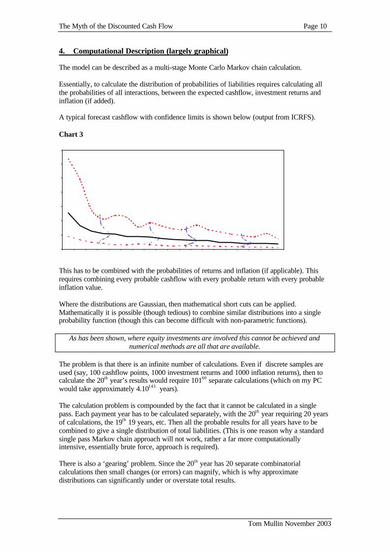
4. Computational Description (largely graphical)

The model can be described as a multi-stage Monte Carlo Markov chain calculation.

Essentially, to calculate the distribution of probabilities of liabilities requires calculating allthe probabilities of all interactions, between the expected cashflow, investment returns andinflation (if added).

A typical forecast cashflow with confidence limits is shown below (output from ICRFS).

Chart 3

This has to be combined with the probabilities of returns and inflation (if applicable). Thisrequires combining every probable cashflow with every probable return with every probableinflation value.

Where the distributions are Gaussian, then mathematical short cuts can be applied.Mathematically it is possible (though tedious) to combine similar distributions into a singleprobability function (though this can become difficult with non-parametric functions).

As has been shown, where equity investments are involved this cannot be achieved andnumerical methods are all that are available.

The problem is that there is an infinite number of calculations. Even if discrete samples areused (say, 100 cashflow points, 1000 investment returns and 1000 inflation returns), then tocalculate the 20th year’s results would require 10160 separate calculations (which on my PCwould take approximately 4.10143 years).

The calculation problem is compounded by the fact that it cannot be calculated in a singlepass. Each payment year has to be calculated separately, with the 20th year requiring 20 yearsof calculations, the 19th 19 years, etc. Then all the probable results for all years have to becombined to give a single distribution of total liabilities. (This is one reason why a standardsingle pass Markov chain approach will not work, rather a far more computationallyintensive, essentially brute force, approach is required).

There is also a ‘gearing’ problem. Since the 20th year has 20 separate combinatorialcalculations then small changes (or errors) can magnify, which is why approximatedistributions can significantly under or overstate total results.



Since this is impossible to do then a Monte Carlo approach is all that is available. This is asimulation technique where random samples of numbers are taken from distributions, thenused for calculation. These samples of numbers are then used to do a Markov chain typecalculation for every payment year. A further Markov chain calculation is then required tocombine every year’s liabilities into a single distribution. These then have to be repeated oftenenough to get a stable result, since every sample will have different values.

Though it is impossible to do all the calculations, it is possible to do enough of them to get astable and reliable result.

The methodology can be outlined as follows:

(1) First design the model. Care must be taken to model the portfolio’s characteristics, suchas premium income scheduling, payment timing, the forecasting error, the distribution ofapplicable investment returns and the distribution of applicable inflation effects.

A portfolio that (say) receives all income at one time, pays only annually and iscompletely invested in cash will require a very different model structure (trivial actually)to one that receives money continuously, pays continuously and is invested in equities.

A short tail portfolio may be as complex as a long-tailed one if cash inflows/outflows anduncertainties are sufficiently large and complex.

(2) Determine the forecasting period and number of periods. Again, an unstable short-tailedportfolio may require as complex a model as a stable long-tailed one.

(3) Input actual distributions that apply. This is one failing of many Dynamic FinancialModels, as they often use assumed distributions.

(4) If Gaussian distributions do apply, then try mathematical short cuts to combinedistributions to reduce the calculations required.

(5) If not Gaussian, then determine the level of discreteness in values used for sampling .Essentially the more coarse the values sampled from a distribution, then the moresimulations that have to be ran and the less stable will be the final result. Then applyMonte Carlo Markov techniques.



5. An Actual Example Using Real Data

The following model was created with these characteristics, choices being limited bycomputational capacity and data availability.

(1) A 20 year annual payment cashflow with an log normal ε and a CV of 40%. Thisforecast cashflow was based on actual workers’ compensation data and used the ICRFSsystem to forecast trends and uncertainties.

(2) Inflation is the same as Australian CPI.

(3) The total premium is invested in Australian equities in indexed funds and premiums werepaid at random times through the year.

(4) The choice of distribution to chose to select out probable investment earning rates was thedaily 20 year All Ordinaries index. The rationale was that:

• It is impossible to predict short and long term earning rates.

• Chaotic systems do exhibit regularity over sufficient time.

• Therefore a sufficiently large period will cover all probabilities of future returns(though we can never actually say when they may occur).

This is probably the most contentious assumption and does require furtherresearch. Is a 20 year history sufficient? Analysis of year to year (over even 3 or 5year) returns show significant differences between periods. Does it require 30 or 40years to capture all probable outcomes?

(5) 30 Simulation runs in total were undertaken, with a sampling of 2,000 points forevery calculation with constant resampling. This meant that the number ofcalculations increased linearly rather than geometrically (approximately 840.106

calculations). With overheads for frequency counts and other statistics beingcalculated at every step meant a single simulation run took approximately 15mins(1Ghz AMD processor), with the full 30 runs taking about 7.5 hours.

Deterministic NPV calculation of mean payments, liability = $24.251 millionWith a ‘safe’ investment earning rate of 2% above CPI, liability = $29.009 millionWith a ‘safe’ investment earning rate of 2.5% above CPI, liability = $28.046 millionWith a ‘safe’ investment earning rate of 3% above CPI, liability = $27.135 million

Stochastic Liability with Actual CPI and earning rates, liability = $29.116 million



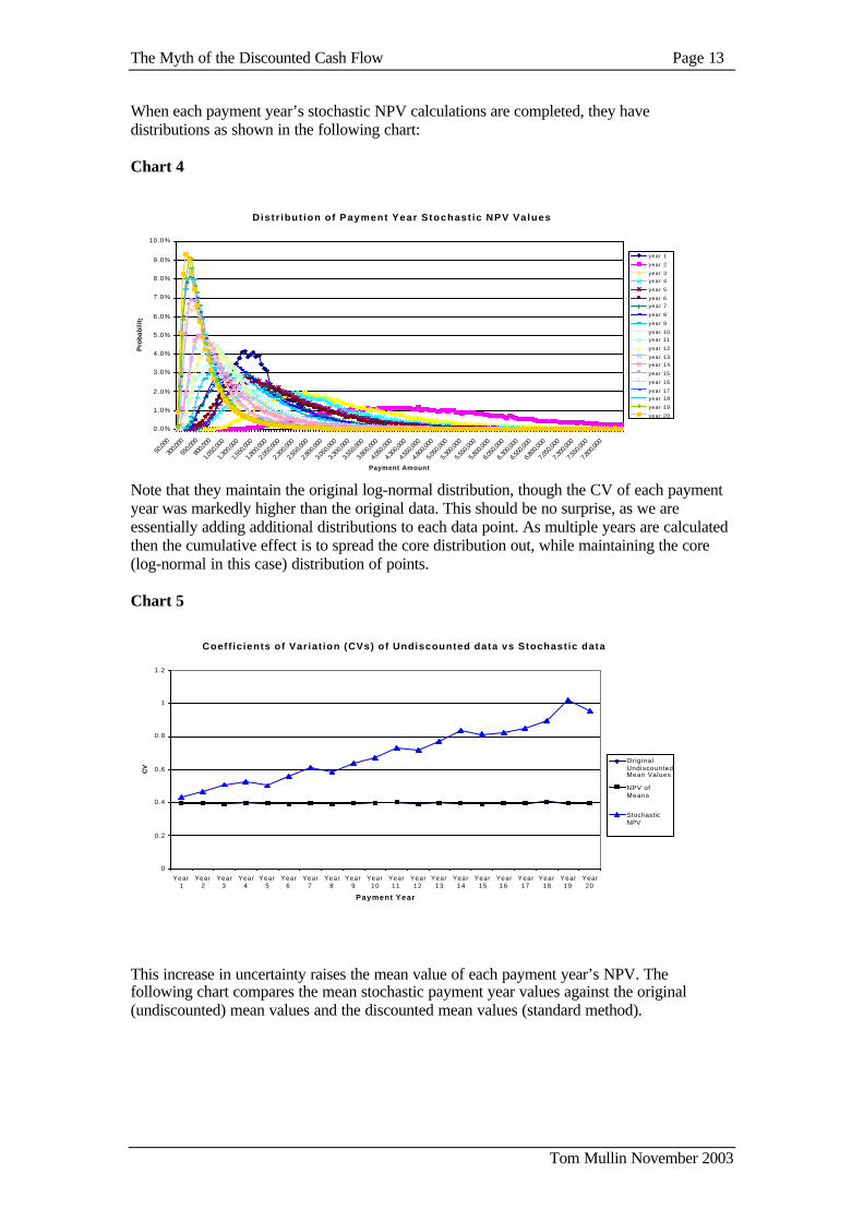
When each payment year’s stochastic NPV calculations are completed, they havedistributions as shown in the following chart:

Chart 4

Note that they maintain the original log-normal distribution, though the CV of each paymentyear was markedly higher than the original data. This should be no surprise, as we areessentially adding additional distributions to each data point. As multiple years are calculatedthen the cumulative effect is to spread the core distribution out, while maintaining the core(log-normal in this case) distribution of points.

Chart 5

This increase in uncertainty raises the mean value of each payment year’s NPV. Thefollowing chart compares the mean stochastic payment year values against the original(undiscounted) mean values and the discounted mean values (standard method).

Distr ibut ion of Payment Year Stochast ic NPV Values

0.0%

1.0%

2.0%

3.0%

4.0%

5.0%

6.0%

7.0%

8.0%

9.0%

10.0%

50,00

0

300,0

00

550,0

00

800,0

00

1,05

0,000

1,30

0,000

1,55

0,000

1,80

0,000

2,05

0,000

2,30

0,000

2,55

0,000

2,80

0,000

3,05

0,000

3,30

0,000

3,55

0,000

3,80

0,000

4,05

0,000

4,30

0,000

4,55

0,000

4,80

0,000

5,05

0,000

5,30

0,000

5,55

0,000

5,80

0,000

6,05

0,000

6,30

0,000

6,55

0,000

6,80

0,000

7,05

0,000

7,30

0,000

7,55

0,000

7,80

0,000

Payment Amount

Pro

bab

ility

year 1

year 2

year 3year 4

year 5

year 6year 7

year 8

year 9

year 10year 11

year 12

year 13year 14

year 15

year 16

year 17year 18

year 19

year 20

Coeff ic ients of Variat ion (CVs) of Undiscounted data vs Stochast ic data

0

0.2

0.4

0.6

0.8

1

1.2

Year1

Year2

Year3

Year4

Year5

Year6

Year7

Year8

Year9

Year10

Year11

Year12

Year13

Year14

Year15

Year16

Year17

Year18

Year19

Year20

Payment Year

CV

OriginalUndiscountedMean Values

NPV ofMeans

StochasticNPV



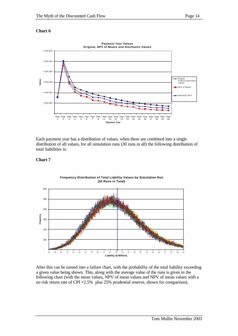
Chart 6

Each payment year has a distribution of values, when these are combined into a singledistribution of all values, for all simulation runs (30 runs in all) the following distribution oftotal liabilities is:

Chart 7

After this can be turned into a failure chart, with the probability of the total liability exceedinga given value being shown. This, along with the average value of the runs is given in thefollowing chart (with the mean values, NPV of mean values and NPV of mean values with ano risk return rate of CPI +2.5% plus 25% prudential reserve, shown for comparison).

Payment Year ValuesOriginal, NPV of Means and Stochastic Values

-

1,000,000

2,000,000

3,000,000

4,000,000

5,000,000

6,000,000

Year1

Year2

Year3

Year4

Year5

Year6

Year7

Year8

Year9

Year10

Year11

Year12

Year13

Year14

Year15

Year16

Year17

Year18

Year19

Year20

Payment Year

Val

ues

OriginalUndiscounted MeanValues

NPV of Means

Stochastic NPV

Frequency Distribution of Total Liabiltiy Values by Simulation Run(30 Runs in Total)

-

100

200

300

400

500

600

18 19 20 21 22 23 24 25 26 27 28 29 30 31 32 33 34 35 36 37 38 39 40

Liability ($ Million)

Fre

qu

ency



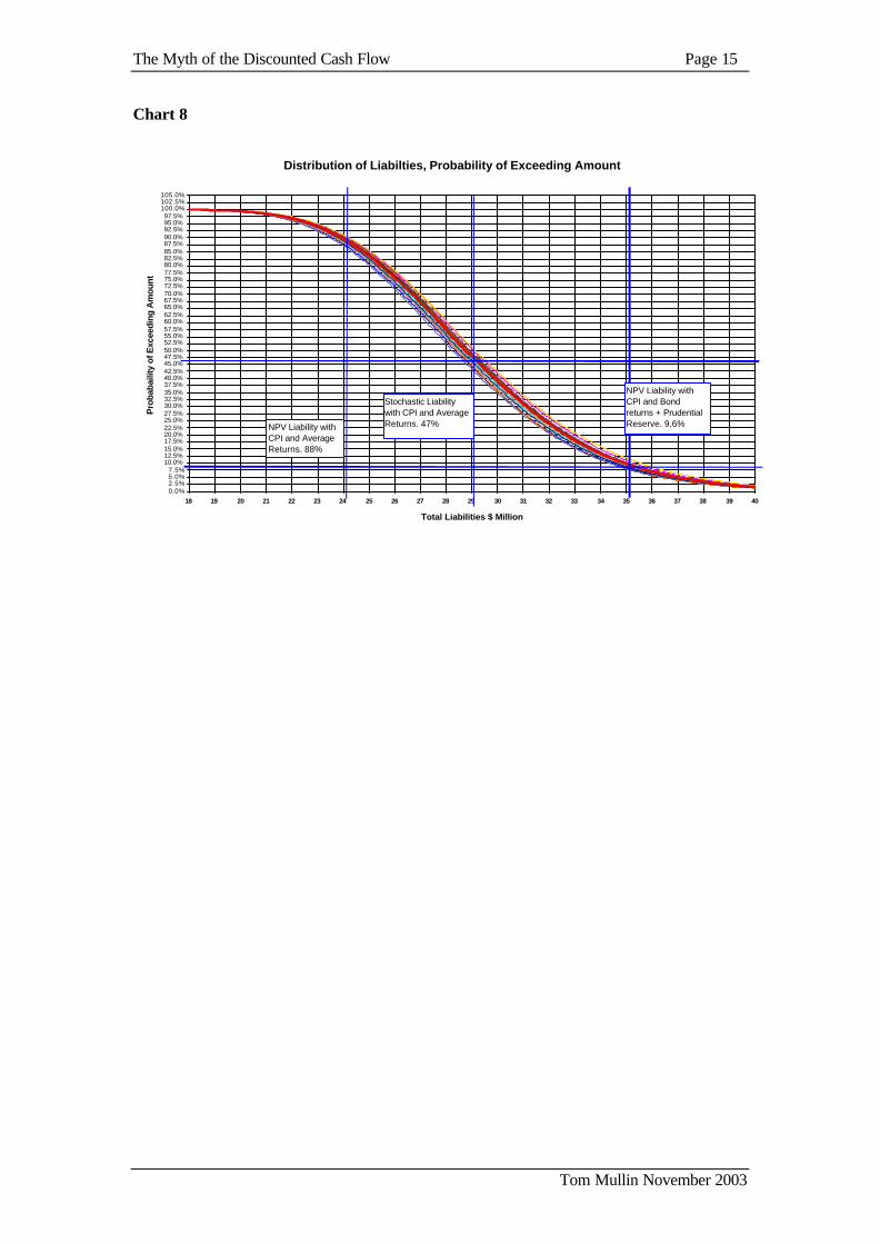
Chart 8

Distribution of Liabilties, Probability of Exceeding Amount

0.0%2.5%5.0%7.5%

10.0%12.5%15.0%17.5%20.0%22.5%25.0%27.5%30.0%32.5%35.0%37.5%40.0%42.5%45.0%47.5%50.0%52.5%55.0%57.5%60.0%62.5%65.0%67.5%70.0%72.5%75.0%77.5%80.0%82.5%85.0%87.5%90.0%92.5%95.0%97.5%

100.0%102.5%105.0%

18 19 20 21 22 23 24 25 26 27 28 29 30 31 32 33 34 35 36 37 38 39 40

Total Liabilities $ Million

Pro

baba

ility

of E

xcee

ding

Am

ount

NPV Liability with CPI and Average Returns. 88%

Stochastic Liability with CPI and Average Returns. 47%

NPV Liability with CPI and Bond returns + Prudential Reserve. 9.6%



6. Comparison of the Probability Distribution of Liabilities to StandardPractises

The stochastic liability values are compared with standard calculations in the following table:

Table 1

Liability Value Liability Valueas % of Mean

value

Probability of Thisor lesser Amount

Occurring

Probability of ThisAmount Being Exceeded

Comment

24,251,379 88.1% 11.8% 88.2% NPV of Mean Values,average CPI & Equityreturns

29,379,952 100.0% 53.2% 46.8% Mean Stochastic LiabilityValue

30,000,000 103.0% 61.1% 38.9%31,000,000 106.5% 69.2% 30.8%

32,000,000 109.9% 76.8% 23.2%

33,000,000 113.3% 82.0% 18.0%

34,000,000 116.8% 86.7% 13.3%

35,057,790 120.4% 90.4% 9.6%

NPV of Mean Values,Average CPI rates. Safeinvestment earning rate ofCPI + 2.5%. 25%Prudential Margin added .

36,000,000 123.6% 93.0% 7.0%37,000,000 127.1% 95.3% 4.9%

38,000,000 130.5% 96.6% 3.4%

39,000,000 133.9% 97.6% 2.4%

40,000,000 137.4% 98.4% 1.6%

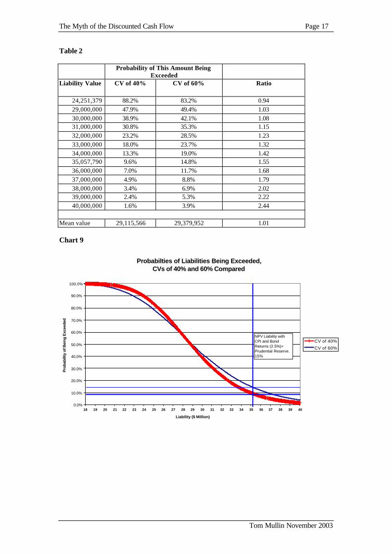
As can be seen there is nearly a 1 in 10 chance of the standard mean value (with a ‘safe’investment rate, plus a prudential margin), being exceeded. There is nearly 1 in 20 chance thatthe mean value will be exceeded by more that 27%.

6.1 Impact of Increasing Payment Forecast Uncertainty

As might be expected the results are sensitive to increases in the uncertainty in the paymentforecast, with failure risks increasing dramatically at higher values. Comparative runs with aforecasting uncertainty increased to 60% (not uncommon) were undertaken

If the CV of the original payment distribution increase to 60% then the mean value onlyincreases by 1%, however the risk of the ‘risk free’ liability being exceeded increases by over50%. The chance that the mean value will be exceeded by more that 27% increases by 80%.



Table 2

Probability of This Amount BeingExceeded

Liability Value CV of 40% CV of 60% Ratio

24,251,379 88.2% 83.2% 0.94 29,000,000 47.9% 49.4% 1.03 30,000,000 38.9% 42.1% 1.08 31,000,000 30.8% 35.3% 1.15 32,000,000 23.2% 28.5% 1.23 33,000,000 18.0% 23.7% 1.32 34,000,000 13.3% 19.0% 1.42 35,057,790 9.6% 14.8% 1.55 36,000,000 7.0% 11.7% 1.68 37,000,000 4.9% 8.8% 1.79 38,000,000 3.4% 6.9% 2.02 39,000,000 2.4% 5.3% 2.22 40,000,000 1.6% 3.9% 2.44

Mean value 29,115,566 29,379,952 1.01

Chart 9

Probabilties of Liabilities Being Exceeded, CVs of 40% and 60% Compared

0.0%

10.0%

20.0%

30.0%

40.0%

50.0%

60.0%

70.0%

80.0%

90.0%

100.0%

18 19 20 21 22 23 24 25 26 27 28 29 30 31 32 33 34 35 36 37 38 39 40

Liability ($ Million)

Pro

babi

lity

of B

eing

Exc

eede

d

CV of 40%

CV of 60%

NPV Liability with CPI and Bond Returns (2.5%)+ Prudential Reserve. 15%



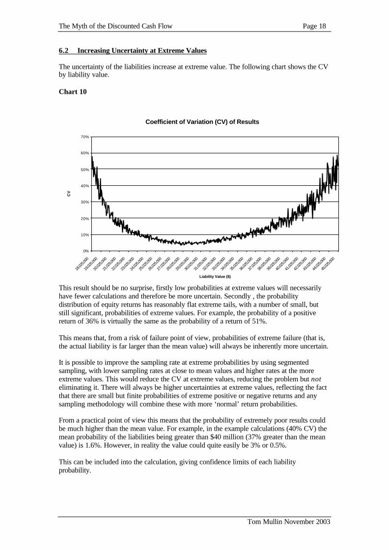
6.2 Increasing Uncertainty at Extreme Values

The uncertainty of the liabilities increase at extreme value. The following chart shows the CVby liability value.

Chart 10

This result should be no surprise, firstly low probabilities at extreme values will necessarilyhave fewer calculations and therefore be more uncertain. Secondly , the probabilitydistribution of equity returns has reasonably flat extreme tails, with a number of small, butstill significant, probabilities of extreme values. For example, the probability of a positivereturn of 36% is virtually the same as the probability of a return of 51%.

This means that, from a risk of failure point of view, probabilities of extreme failure (that is,the actual liability is far larger than the mean value) will always be inherently more uncertain.

It is possible to improve the sampling rate at extreme probabilities by using segmentedsampling, with lower sampling rates at close to mean values and higher rates at the moreextreme values. This would reduce the CV at extreme values, reducing the problem but noteliminating it. There will always be higher uncertainties at extreme values, reflecting the factthat there are small but finite probabilities of extreme positive or negative returns and anysampling methodology will combine these with more ‘normal’ return probabilities.

From a practical point of view this means that the probability of extremely poor results couldbe much higher than the mean value. For example, in the example calculations (40% CV) themean probability of the liabilities being greater than $40 million (37% greater than the meanvalue) is 1.6%. However, in reality the value could quite easily be 3% or 0.5%.

This can be included into the calculation, giving confidence limits of each liabilityprobability.

Coefficient of Variation (CV) of Results

0%

10%

20%

30%

40%

50%

60%

70%

18,02

5,000

19,02

5,000

20,02

5,000

21,02

5,000

22,02

5,000

23,02

5,000

24,02

5,000

25,02

5,000

26,02

5,000

27,02

5,000

28,02

5,000

29,02

5,000

30,02

5,000

31,02

5,000

32,02

5,000

33,02

5,000

34,02

5,000

35,02

5,000

36,02

5,000

37,02

5,000

38,02

5,000

39,02

5,000

40,02

5,000

41,02

5,000

42,02

5,000

43,02

5,000

44,02

5,000

45,02

5,000

Liability Value ($)

CV



6.3 Combining Multiple Injury Years and/or Product Lines

The example shown is for a single injury year, but in principle combining multiple injuryyears results, which can then be used for a stochastic NPV calculation, is straightforward.

• Where multiple injury years exhibit the same type of error(ε ) distribution (e.g. lognormal) then combining payments years (at the same point of development) distributions(albeit with different means and standard deviations) is trivial.

• Where error distributions differ in type, they can be combined using numerical methods.

• The same principles apply to combining different product lines, though caution should beapplied as it t may be advantageous to model widely differing products separately toenable better investment portfolio matching.

• The decision to combine/split stochastic NPV calculations of different products may beanother fruitful area of research to determine the optimum splits and combinations thatshould be made (e.g. all short tail combined, all long tail combined).



7. Conclusions and Future Research to be Completed

7.1 Conclusions

• The methodology outlined of applying stochastic principles to NPV calculations is valid.

• It is capable of handling chaotic equity returns, which few other methodologies attemptwithout resorting to unfounded assumptions.

• It can be expanded to mixed investment portfolios as well as other investment types (suchas overseas equities).

• The True Risk of investment portfolios not meeting liabilities can be calculated, alongwith the uncertainty of the calculation.

• This enables rational decisions to be made about the risk/returns that organisations wishto undertake.

• The methodology is computationally demanding but well within the reach of mostorganisations (additionally it is ideal for concurrent processing, with multiple processorsor PCs calculating separate sections then results being combined). It does vastly exceedthe capacity of any spreadsheet and would be difficult to undertake in a macro basedlanguage such as SAS. Any 3rd generation programming language (such as C) would besuitable (albeit after ensuring that high precision is available) though scientific basedlanguages such as Fortran or APL are more suitable, due to the need to manipulate verylarge matrices. It is essential that any language (or version/compiler) used has a goodrandom number generator.

7.2 Further Research to be Undertaken

• Further research needs to be undertaken on determining the optimum number of years ofequity returns to cover all probabilities that are appropriate for a given calculation.

• Further research to determine the optimum splits and combinations of product lines thatshould be made (e.g. all short tail combined, all long tail combined).

• What proportion of equities is required to have a noticeable chaotic effect on a mixedinvestment portfolio?

• Other investment types (such as overseas equities raising the additional issue of exchangerate uncertainty) need to be researched.

• Low cashflow uncertainty product lines (e.g. life insurance, where the cashflowuncertainty comes from sampling uncertainty from a population mortality table) need tobe investigated.

• Further work needs to be undertaken to investigate segmented sampling to reduce (butwont eliminate) high CVs for extreme values.

• The balance between sampling coarseness, number of simulations and result stabilityneeds to be researched to determine the best selections for optimum run time and resultstability.



7.3 Caveat

A stochastic cashflow forecasting methodology (such as Insureware’s ICRFS forecastingsystem) is essential.

If forecast cashflow uncertainty cannot be calculated then this methodology cannot beapplied, therefore standard industry techniques, such as chain-ladder/ratio forecasting

models, are inapplicable.

Documents

The Myth of the Discounted Cash Flow #2 - Actuaries