The Multinomial Model∗

STA 312: Fall 2012

Contents

1 Multinomial Coefficients 1

2 Multinomial Distribution 2

3 Estimation 4

4 Hypothesis tests 8

5 Power 17

1 Multinomial Coefficients

Multinomial coefficient For c categoriesFrom n objects, number of ways to choose

• n1 of type 1

• n2 of type 2...

• nc of type c

(n

n1 · · · nc

)=

n!

n1! · · · nc!

∗See last slide for copyright information.

1

Example of a multinomial coefficient A counting problemOf 30 graduating students, how many ways are there for 15 to be employed in a job

related to their field of study, 10 to be employed in a job unrelated to their field of study,and 5 unemployed? (

30

15 10 5

)= 465, 817, 912, 560

2 Multinomial Distribution

Multinomial Distribution Denote by M(n,π), where π = (π1, . . . , πc)

• Statistical experiment with c outcomes

• Repeated independently n times

• Pr(Outcome j) = πj, j = 1, . . . , c

• Number of times outcome j occurs is nj, j = 1, . . . , c

• An integer-valued multivariate distribution

P (n1, . . . , nc) =

(n

n1 · · · nc

)πn11 · · · πncc ,

where 0 ≤ nj ≤ n,c∑j=1

nj = n, 0 < πj < 1, andc∑j=1

πj = 1.

There are actually c− 1 variables and c− 1 parameters In the multinomial withc categories

P (n1, . . . , nc−1) =n!

n1! · · · nc−1!(n−∑c−1

j=1 nj)!

× πn11 · · · π

nc−1

c−1 (1−c−1∑j=1

πj)n−

∑c−1j=1 nj

2

Marginals of the multinomial are multinomial too Add over nc−1, which goesfrom zero to whatever is left over from the other counts.

n−∑c−2

j=1nj∑

nc−1=0

n!

n1! . . . nc−1!(n−∑c−1

j=1 nj)!πn11 · · ·π

nc−1c−1 (1 −

c−1∑j=1

πj)n−

∑c−1j=1

nj ×(n−

∑c−2j=1 nj)!

(n−∑c−2

j=1 nj)!

=n!

n1! . . . nc−2!(n−∑c−2

j=1 nj)!πn11 · · ·π

nc−2c−2

×

n−∑c−2

j=1nj∑

nc−1=0

(n−∑c−2

j=1 nj)!

nc−1!(n−∑c−2

j=1 nj − nc−1)!πnc−1c−1 (1 −

c−2∑j=1

πj − πc−1)n−

∑c−2j=1

nj−nc−1

=n!

n1! . . . nc−2!(n−∑c−2

j=1 nj)!πn11 · · ·π

nc−2c−2 (1 −

c−2∑j=1

πj)n−

∑c−2j=1

nj ,

where the last equality follows from the Binomial Theorem. It’s multinomial with c− 1categories.

Observe You are responsible for these implications of the last slide.

• Adding over nc−1 throws it into the last (“leftover”) category.

• Labels 1, . . . , c are arbitrary, so this means you can combine any 2 categories and theresult is still multinomial.

• c is arbitrary, so you can keep doing it and combine any number of categories.

• When only two categories are left, the result is binomial

• E(nj) = nπj = µj, V ar(nj) = nπj(1− πj)

Sample problem Recent university graduates

• Probability of job related to field of study = 0.60

• Probability of job unrelated to field of study = 0.30

• Probability of no job = 0.10

Of 30 randomly chosen students, what is probability that 15 are employed in a job relatedto their field of study, 10 are employed in a job unrelated to their field of study, and 5 areunemployed?(

30

15 10 5

)0.60150.30100.105 =

4933527642332542053801

381469726562500000000000≈ 0.0129

What is the probability that exactly 5 are unemployed?(30

5 25

)0.1050.9025 =

51152385317007572507646551997

500000000000000000000000000000≈ 0.1023

3

Conditional probabilities are multinomial too

• Given that a student finds a job, what is the probability that the job will be in thestudent’s field of study?

P (Field|Job) =P (Field, Job)

P (Job)=

0.60

0.90=

2

3

• Suppose we choose 50 students at random from those who found jobs. What is theprobability that exactly y of them will be employed in their field of study, for y =0, . . . , 50?

P (y|Job) =

(50

y

)(2

3

)y (1− 2

3

)50−y

Calculating multinomial probabilities with ROf 30 randomly chosen students, what is probability that 15 are employed in a job related

to their field of study, 10 are employed in a job unrelated to their field of study, and 5 areunemployed?(

30

15 10 5

)0.60150.30100.105 =

4933527642332542053801

381469726562500000000000≈ 0.0129

> dmultinom(c(15,10,5), prob=c(.6, .3, .1))

[1] 0.01293295

3 Estimation

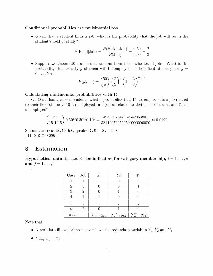
Hypothetical data file Let Yi,j be indicators for category membership, i = 1, . . . , nand j = 1, . . . , c

.

Case Job Y1 Y2 Y3

1 1 1 0 02 3 0 0 13 2 0 1 04 1 1 0 0...

......

......

n 2 0 1 0

Total∑n

i=1 yi,1∑n

i=1 yi,2∑n

i=1 yi,3

Note that

• A real data file will almost never have the redundant variables Y1, Y2 and Y3.

•∑n

i=1 yi,j = nj

4

Lessons from the data file

• Cases (n of them) are independent M(1,π), so E(Yi,j) = πj.

• Column totals nj count the number of times each category occurs: Joint distributionis M(n,π)

• If you make a frequency table (frequency distribution)

– The nj counts are the cell frequencies!

– They are random variables, and now we know their joint distribution.

– Each individual (marginal) table frequency is B(n, πj).

– Expected value of cell frequency j is E(nj) = nπj = µj

• Tables of 2 and or more dimensions present no problems; form combination variables.

Example of a frequency table For the Jobs data

Job Category Frequency PercentEmployed in field 106 53Employed outside field 74 37Unemployed 20 10Total 200 100.0

Likelihood function for the multinomial

`(π) =n∏i=1

Pr{Yi,1 = yi,1, Yi,2 = yi,2, . . . , Yi,c = yi,c|π}

=n∏i=1

πyi,11 π

yi,22 · · · πyi,cc

= π∑ni=1 yi,1

1 π∑ni=1 yi,2

2 · · · π∑ni=1 yi,c

c

= πn11 π

n22 · · · πncc

• Product of n probability mass functions, each M(1,π)

• Depends upon the sample data only through the vector of c frequency counts: (n1, . . . , nc)

5

All you need is the frequency table

`(π) = πn11 π

n22 · · · πncc

• Likelihood function depends upon the sample data only through the frequency counts.

• By the factorization theorem, (n1, . . . , nc) is a sufficient statistic.

• All the information about the parameter in the sample data is contained in the sufficientstatistic.

• So everything the sample data could tell you about (π1, . . . , πc) is given by in (n1, . . . , nc).

• You don’t need the raw data.

Log likelihood: c− 1 parameters

`(π) = πn11 · · · πncc

= πn11 · · · π

nc−1

c−1

(1−

c−1∑j=1

πj

)n−∑c−1j=1 nj

log `(π) =c−1∑j=1

nj log πj +

(n−

c−1∑j=1

nj

)log

(1−

c−1∑j=1

πj

)

∂ log `

∂πj=njπj− n−

∑c−1k=1 nk

1−∑c−1

k=1 πk, for j = 1, . . . , c− 1

Set all the partial derivatives to zero and solve For πj, j = 1 . . . , c-1

π̂j =njn

= pj =

∑ni=1 yi,jn

= yj

So the MLE is the sample proportion, which is also a sample mean.

6

In matrix terms: π̂ = p = Yn π̂1...

π̂c−1

=

p1...

pc−1

=

Y 1...

Y c−1

Remarks:

• Multivariate Law of Large Numbers says pp→ π

• Multivariate Central Limit Theorem says that Yn is approximately multivariate normalfor large n.

• Because nj ∼ B(n, πj),njn

= Y j = pj is approximately N(πj,

πj(1−πj)n

).

• Approximate πj with pj in the variance if necessary.

• Can be used in confidence intervals and tests about a single parameter.

• We have been using c− 1 categories only for technical convenience.

Confidence interval for a single parameter 95% confidence interval for true pro-portion unemployed

Job Category Frequency PercentEmployed in field 106 53Employed outside field 74 37Unemployed 20 10Total 200 100.0

p3approx∼ N

(π3,

π3(1− π3)n

)So a confidence interval is

p3 ± 1.96

√p3(1− p3)

n= 0.20± 1.96

√0.10(1− 0.10)

200= 0.10± 0.042

= (0.058, 0.242)

7

4 Hypothesis tests

For general tests on multinomial dataWe will use mostly

• Pearson chi-squared tests

• Large-sample likelihood ratio tests

There are other possibilities, including

• Wald tests

• Score tests

All these are large-sample chi-squared tests, justified as n→∞

Likelihood ratio tests In generalSetup

Y1, . . . , Yni.i.d.∼ Fβ, β ∈ B,

H0 : β ∈ B0 v.s. H1 : β ∈ B1 = B ∩ Bc0Test Statistic:

G2 = −2 log

(maxβ∈B0 `(β)

maxβ∈B `(β)

)= −2 log

(`0`1

)

What to do And how to think about it

G2 = −2 log

(maxβ∈B0 `(β)

maxβ∈B `(β)

)= −2 log

(`0`1

)• Maximize the likelihood over the whole parameter space. You already did this to

calculate the MLE. Evaluate the likelihood there. That’s the denominator.

• Maximize the likelihood over just the parameter values where H0 is true – that is, overB0. This yields a restricted MLE. Evaluate the likelihood there. That’s the numerator.

• The numerator cannot be larger, because B0 ⊂ B.

• If the numerator is a lot less than the denominator, the null hypothesis is unbelievable,and

– The ratio is close to zero

– The log of the ratio is a big negative number

– −2 times the log is a big positive number

– Reject H0 when G2 is large enough.

8

Distribution of G2 under H0

Given some technical conditions,

• G2 has an approximate chi-squared distribution under H0 for large n.

• Degrees of freedom equal number of (non-redundant) equalities specified by H0.

• Reject H0 when G2 is larger than the chi-squared critical value.

Counting degrees of freedom

• Express H0 as a set of linear combinations of the parameters, set equal to constants(usually zeros for regression problems).

• Degrees of freedom = number of non-redundant (linearly independent) linear combi-nations.

Suppose β = (β1, . . . β7), withH0 : β1 = β2, β6 = β7,

13

(β1 + β2 + β3) = 13

(β4 + β5 + β6)Then df = 3: Count the equals signs.But if β1 = β2 = β3 = β4 = β5 = β6 = β7 = 1

7, then df = 6

ExampleUniversity administrators recognize that the percentage of students who are unemployed

after graduation will vary depending upon economic conditions, but they claim that still,about twice as many students will be employed in a job related to their field of study,compared to those who get an unrelated job. To test this hypothesis, they select a randomsample of 200 students from the most recent class, and observe 106 employed in a jobrelated to their field of study, 74 employed in a job unrelated to their field of study, and 20unemployed. Test the hypothesis using a large-sample likelihood ratio test and the usual0.05 significance level State your conclusions in symbols and words.

Some detailed questions To guide us through the problem

• What is the model?Y1, . . . , Yn

i.i.d.∼ M(1, (π1, π2, π3))

• What is the null hypothesis, in symbols?

H0 : π1 = 2π2

• What are the degrees of freedom for this test?

1

9

What is the parameter space B? What is the restricted parameter space B0?

0.0 0.2 0.4 0.6 0.8 1.0

0.0

0.2

0.4

0.6

0.8

1.0

π1

π 2

B = {(π1, π2) : 0 < π1 < 1, 0 < π2 < 1, π1 + π2 < 1}B0 = {(π1, π2) : 0 < π1 < 1, 0 < π2 < 1, π1 = 2π2}

What is the unrestricted MLE?Give the answer in both symbolic and numerical form. Just write it down. There is no

need to show any work.

p = (n1

n,n2

n,n3

n)

= (106

200,

74

200,

20

200)

= (0.53, 0.37, 0.10)

Derive the restricted MLEYour answer is a symbolic expression. It’s a vector. Show your work.

10

∂

∂π(n1 log(2π) + n2 log π + n3 log(1− 3π))

=n1

π+n2

π+

n3

1− 3π(−3)

set= 0

⇒ n1 + n2

π=

3n3

1− 3π⇒ (n1 + n2)(1− 3π) = 3πn3

⇒ n1 + n2 = 3π(n1 + n2 + n3) = 3πn

⇒ π =n1 + n2

3n

So π̂ =(

2(n1+n2)3n

, n1+n2

3n, n3

n

). From now on, π̂ means the restricted MLE.

Give the restricted MLE in numeric form The answer is a vector of 3 numbers

π̂ =

(2(n1 + n2)

3n,n1 + n2

3n,n3

n

)=

(2(106 + 74)

600,106 + 74

600,

20

200

)= (0.6, 0.3, 0.1)

Show the restricted and unrestricted MLEs Restricted is black diamond, unre-stricted is red circle

0.0 0.2 0.4 0.6 0.8 1.0

0.0

0.2

0.4

0.6

0.8

1.0

π1

π 2

11

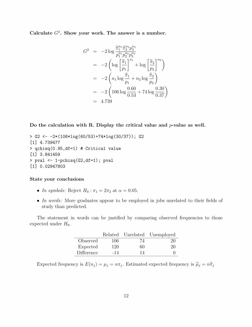
Calculate G2. Show your work. The answer is a number.

G2 = −2 logπ̂n11 π̂

n22 p

n33

pn11 p

n22 p

n33

= −2

(log

[π̂1p1

]n1

+ log

[π̂2p2

]n2)

= −2

(n1 log

π̂1p1

+ n2 logπ̂2p2

)= −2

(106 log

0.60

0.53+ 74 log

0.30

0.37

)= 4.739

Do the calculation with R. Display the critical value and p-value as well.

> G2 <- -2*(106*log(60/53)+74*log(30/37)); G2

[1] 4.739477

> qchisq(0.95,df=1) # Critical value

[1] 3.841459

> pval <- 1-pchisq(G2,df=1); pval

[1] 0.02947803

State your conclusions

• In symbols : Reject H0 : π1 = 2π2 at α = 0.05.

• In words : More graduates appear to be employed in jobs unrelated to their fields ofstudy than predicted.

The statement in words can be justified by comparing observed frequencies to thoseexpected under H0.

Related Unrelated UnemployedObserved 106 74 20Expected 120 60 20

Difference -14 14 0

Expected frequency is E(nj) = µj = nπj. Estimated expected frequency is µ̂j = nπ̂j

12

Write G2 in terms of observed and expected frequencies For a general hypothesisabout a multinomial

G2 = −2 log

(`0`1

)= −2 log

(∏cj=1 π̂

njj∏c

j=1 pnjj

)

= −2 logk∏j=1

(π̂jpj

)nj= 2

c∑j=1

− log

(π̂jpj

)xj= 2

c∑j=1

nj log

(π̂jpj

)−1= 2

c∑j=1

nj log

(pjπ̂j

)

= 2c∑j=1

nj log

(njnπ̂j

)= 2

c∑j=1

nj log

(njµ̂j

)

Likelihood ratio test for the multinomial Jobs data

G2 = 2c∑j=1

nj log

(njnπ̂j

)= 2

c∑j=1

nj log

(njµ̂j

)

> freq = c(106,74,20); n = sum(freq)

> pihat = c(0.6,0.3,0.1); muhat = n*pihat

> G2 = 2 * sum(freq*log(freq/muhat)); G2

[1] 4.739477

Pearson’s chi-squared test Comparing observed and expected frequencies

X2 =

c∑j=1

(nj − µ̂j)2

µ̂j

where µ̂j = nπ̂j

• A large value means the observed frequencies are far from what is expected given H0.

13

• A large value makes H0 less believable.

• Distributed approximately as chi-squared for large n if H0 is true.

Pearson Chi-squared on the jobs data

Observed 106 74 20Expected 120 60 20

X2 =c∑j=1

(nj − µ̂j)2

µ̂j

=(106− 120)2

120+

(74− 60)2

60+ 0

= 4.9 (Compare G2 = 4.74)

Two chi-squared test statistics There are plenty more.

G2 = 2c∑j=1

nj log

(njµ̂j

)X2 =

c∑j=1

(nj − µ̂j)2

µ̂j

• Both compare observed to expected frequencies.

• By expected we mean estimated expected: µ̂j = nπ̂j.

• Both equal zero when all observed frequencies equal the corresponding expected fre-quencies.

• Both have approximate chi-squared distributions with the same df when H0 is true,for large n.

• Values are close for large n when H0 is true.

• Both go to infinity when H0 is false.

• X2 works better for smaller samples.

• X2 is specific to multinomial data; G2 is more general.

14

Rules of thumb

• Small expected frequencies can create trouble by inflating the test statistic.

• G2 is okay if all (estimated) expected frequencies are at least 5.

• X2 is okay if all (estimated) expected frequencies are at least 1.

One more example: Is a die fair?Roll the die 300 times and observe these frequencies:

1 2 3 4 5 672 39 54 44 44 47

• State a reasonable model for these data.

• Without any derivation, estimate the probability of rolling a 1. Your answer is a number.

• Give an approximate 95% confidence interval for the probability of rolling a 1. Your answeris a set of two numbers.

• What is the null hypothesis corresponding to the main question, in symbols?

• What is the parameter space B?

• What is the restricted parameter space B0?

• What are the degrees of freedom? The answer is a number.

• What is the critical value of the test statistic at α = 0.05? The answer is a number.

Questions continued

• What are the expected frequencies under H0? Give 6 numbers.

• Carry out the likelihood ratio test.

– What is the value of the test statistic? Your answer is a number. Show somework.

– Do you reject H0 at α = 0.05? Answer Yes or No.

– Using R, calculate the p-value.

– Do the data provide convincing evidence against the null hypothesis?

• Carry out Pearson test. Answer the same questions you did for the likelihood ratiotest.

15

More questions To help with the plain language conclusion

• Does the confidence interval for π1 allow you to reject H0 : π1 = 16

at α = 0.05? AnswerYes or No.

• In plain language, what do you conclude from the test corresponding to the confidenceinterval? (You need not actually carry out the test.)

• Is there evidence that the chances of getting 2 through 6 are unequal? This questionrequires its own slide.

Is there evidence that the chances of getting 2 through 6 are unequal?

• What is the null hypothesis?

• What is the restricted parameter space B0? It’s convenient to make the first categorythe residual category.

• Write the likelihood function for the restricted model. How many free parameters arethere in this model?

• Obtain the restricted MLE π̂. Your final answer is a set of 6 numbers.

• Give the estimated expected frequencies (µ̂1, . . . , µ̂6).

• Calculate the likelihood ratio test statistic. Your answer is a number.

Questions continued

• What are the degrees of freedom of the test? The answer is a number.

• What is the critical value of the test statistic at α = 0.05? The answer is a number.

• Do you reject H0 at α = 0.05? Answer Yes or No.

• In plain language, what (if anything) do you conclude from the test.

• In plain language, what are your overall conclusion about this die?

For most statistical analyses, your final conclusions should be regarded as hypothesesthat need to be tested on a new set of data.

16

5 Power

Power and sample size Using the non-central chi-squared distributionIf X ∼ N(µ, σ2), then

• Z =(X−µσ

)2 ∼ χ2(1)

• Y = X2

σ2 is said to have a non-central chi-squared distribution with degrees of freedom

one and non-centrality parameter λ = µ2

σ2 .

• Write Y ∼ χ2(1, λ)

Facts about the non-central chi-squared distribution With one df

Y ∼ χ2(1, λ), where λ ≥ 0• Pr{Y > 0} = 1, of course.

• If λ = 0, the non-central chi-squared reduces to the ordinary central chi-squared.

• The distribution is “stochastically increasing” in λ, meaning that if Y1 ∼ χ2(1, λ1) andY2 ∼ χ2(1, λ2) with λ1 > λ2, then Pr{Y1 > y} > Pr{Y2 > y} for any y > 0.

• limλ→∞ Pr{Y > y} = 1

• There are efficient algorithms for calculating non-central chi-squared probabilities. R’spchisq function does it.

An example Back to the coffee taste test

Y1, . . . , Yni.i.d.∼ B(1, π)

H0 : π = π0 = 12

Reject H0 if |Z2| =∣∣∣∣√n(p−π0)√

p(1−p)

∣∣∣∣ > zα/2

Suppose that in the population, 60% of consumers would prefer the new blend. If we test100 consumers, what is the probability of obtaining results that are statistically significant?

That is, if π = 0.60, what is the power with n = 100?

17

Recall that if X ∼ N(µ, σ2), then X2

σ2 ∼ χ2(1, µ2

σ2 ).Reject H0 if

|Z2| =

∣∣∣∣∣√n(p− π0)√p(1− p)

∣∣∣∣∣ > zα/2 ⇔ Z22 > z2α/2 = χ2

α(1)

For large n, X = p− π0 is approximately normal, with µ = π − π0 and σ2 = π(1−π)n

. So,

Z22 =

(p− π0)2

p(1− p)/n≈ (p− π0)2

π(1− π)/n=X2

σ2

approx∼ χ2

(1, n

(π − π0)2

π(1− π)

)

We have found thatThe Wald chi-squared test statistic of H0 : π = π0

Z22 =

n(p− π0)2

p(1− p)

has an asymptotic non-central chi-squared distribution with df = 1 and non-centrality pa-rameter

λ = n(π − π0)2

π(1− π)

Notice the similarity, and also that

• If π = π0, then λ = 0 and Z22 has a central chi-squared distribution.

• The probability of exceeding any critical value (power) can be made as large as desiredby making λ bigger.

• There are 2 ways to make λ bigger.

Power calculation with R For n = 100, π0 = 0.50 and π = 0.60

> # Power for Wald chisquare test of H0: pi=pi0

> n=100; pi0=0.50; pi=0.60

> lambda = n * (pi-pi0)^2 / (pi*(1-pi))

> critval = qchisq(0.95,1)

> power = 1-pchisq(critval,1,lambda); power

[1] 0.5324209

18

General non-central chi-squaredLet X1, . . . , Xn be independent N(µi, σ

2i ). Then

Y =n∑i=1

X2i

σ2i

∼ χ2(n, λ), where λ =n∑i=1

µ2i

σ2i

• Density is a bit messy

• Reduces to central chi-squared when λ = 0.

• Generalizes to Y ∼ χ2(ν, λ), where ν > 0 as well as λ > 0

• Stochastically increasing in λ, meaning Pr{Y > y} can be increased by increasing λ.

• limλ→∞ Pr{Y > y} = 1

• Probabilities are easy to calculate numerically.

Non-centrality parameters for Pearson and likelihood Ratio chi-squared testsRe-writing the test statistics in terms of pj . . .

X2 = nc∑j=1

(pj − π̂j)2

π̂jλ = n

c∑j=1

[πj − πj(M)]2

πj(M)

G2 = 2nc∑j=1

pj log

(pjπ̂j

)λ = 2n

c∑j=1

πj log

(πj

πj(M)

),

• Where π̂j → πj(M) as n→∞ under the “model” H0.

• That is, πj(M) is the large-sample target of the restricted MLE.

• The technical meaning is convergence in probability, or π̂jp→ πj(M)

• πj(M) is a function of π1, . . . , πc. Sometimes, πj(M) = πj

For the fair (?) die exampleSuppose we want to test whether the die is fair, but it is not. The true π =

(213, 213, 313, 213, 213, 213

).

What is the power of the Pearson chi-squared test for n = 300?Because B0 = {(1

6, 16, 16, 16, 16)}, It’s easy to see πj(M) = 1

6.

19

λ = nc∑j=1

[πj − πj(M)]2

πj(M)

= 300

(( 313− 1

6)2

16

+ 5( 213− 1

6)2

16

)= 8.87574

Calculate power with R

> piM = 1/6 + numeric(6); piM

[1] 0.1666667 0.1666667 0.1666667 0.1666667 0.1666667 0.1666667

> pi = c(2,2,3,2,2,2)/13; pi

[1] 0.1538462 0.1538462 0.2307692 0.1538462 0.1538462 0.1538462

> lambda = 300 * sum( (pi-piM)^2/piM ); lambda

[1] 8.87574

> critval = qchisq(0.95,5); critval

[1] 11.0705

> power = 1-pchisq(critval,5,lambda); power

[1] 0.6165159

Calculate required sample size To detect π =(

213, 213, 313, 213, 213, 213

)as unfair with

high probabilityPower of 0.62 is not too impressive. How many times would you have to roll the die to

detect this degree of unfairness with probability 0.90?

> piM = 1/6 + numeric(6)

> pi = c(2,2,3,2,2,2)/13

> critval = qchisq(0.95,5)

>

> n = 0; power = 0.05

> while(power < 0.90)

+ { n = n+1

+ lambda = n * sum( (pi-piM)^2/piM )

+ power = power = 1-pchisq(critval,5,lambda)

+ }

> n; power

[1] 557

[1] 0.9001972

20

Sometimes, finding π(M) is more challenging Recall the Jobs example, withH0 : π1 = 2π2

π̂ =

(2(n1 + n2)

3n,n1 + n2

3n,n3

n

)=

(2

3

(n1

n+n2

n

),1

3

(n1

n+n2

n

),n3

n

)=

(2

3(p1 + p2) ,

1

3(p1 + p2) , p3

)p→(

2

3(π1 + π2) ,

1

3(π1 + π2) , π3

)By the Law of Large Numbers.

Copyright InformationThis slide show was prepared by Jerry Brunner, Department of Statistics, University of

Toronto. It is licensed under a Creative Commons Attribution - ShareAlike 3.0 Unported Li-cense. Use any part of it as you like and share the result freely. The LATEX source code is avail-able from the course website: http://www.utstat.toronto.edu/∼brunner/oldclass/312f12

21