The Multi-Fractal Model of Asset Returns:

Its Estimation via GMM and Its Use for Volatility Forecasting

Thomas Lux*

Abstract: Multi-fractal processes have been proposed as a new formalism for modeling the time series of returns in finance. The major attraction of these processes is their ability to generate various degrees of long memory in different powers of returns - a feature that has been found to characterize virtually all financial prices. Furthermore, elementary variants of multi-fractal models are very parsimonious formalizations as they are essentially one-parameter families of stochastic processes. The aim of this paper is to provide the characteristics of a causal multi-fractal model (replacing the earlier combinatorial approaches discussed in the literature), to estimate the parameters of this model and to use these estimates in forecasting financial volatility. We use the auto-covariances of log increments of the multi-fractal process in order to estimate its parameters consistently via GMM (Generalized Method of Moment). Simulations show that this approach leads to essentially unbiased estimates, which also have much smaller root mean squared errors than those obtained from traditional ‘scaling’ approach. Our empirical estimates are used in out-of-sample forecasting of volatility for a number of important financial assets. Comparing the multi-fractal forecasts with those derived from GARCH and FIGARCH models yields results in favor of the new model: multi-fractal forecasts dominate all other forecasts in one out of four cases considered, while in the remaining cases they are head to head with one or more of their competitors. Keywords: multi-fractality, financial volatility, forecasting JEL classification: C20, G12

* Earlier versions of this paper have been presented at the International Conference on Long-Range Dependent Stochastic Processes and their Applications, Indian Institute of Science, Bangalore, 7 – 12 January 2002, the International Conference on Economics and Physics, Denpasar, 28 - 31 August, 2002, the Second ISM/SEKONDAI Economics Meeting, Institute of Statistical Mathematics, Tokyo, 11 November 2002 and the Second Symposium on Financial Fluctuations at Nihon Keizai Nikkei Corp., Tokyo, 12 – 14 November 2002. The author is indebted to many colleagues and participants of these events for their helpful comments. Particular thanks go to two JBES referees and editor-in-charge Alistair Hall for their most useful comments and suggestions, and to Hwa-Taek Lee and Simone Alfarano for their able research assistance. The present version of this paper has been completed during a sabbatical stay at International Christian University Tokyo whose great hospitality is gratefully acknowledged. The author also gratefully appreciates financial support by the Landeszentralbank Schleswig-Holstein and the Japan Society for the Promotion of Science.

February 2003 Address of author: Department of Economics, University of Kiel, Olshausenstr. 40, 24118 Kiel, Germany lux@bwl.uni-kiel.de

2

1. Introduction

While so-called uni-fractal or self-similar processes, such as fractional Brownian motion, have been

known for quite some time in empirical finance, more general multi-fractal processes have been considered

only very recently. After some earlier attempts at recovering traces of multi-fractal behavior (Vassilicos,

Demos and Tata, 1993, Ghasghaie, S. et al., 1996) this topic has also been taken up in a couple of recent

papers. Among these contributions, Schmitt, Schertzer and Lovejoy (1999) and Vandewalle and Ausloos

(1998a, b) concentrate on statistical analyses suggesting the multi-fractal nature of various financial records.

Mandelbrot, Fisher and Calvet (1997), Mandelbrot (1999) and Calvet and Fisher (2002a) proceed one

step further by proposing a compound stochastic process as a generating mechanism of stock returns and

exchange rate changes in which a multi-fractal cascade plays the role of a time transformation. The message

of these papers is unequivocal in indicating that the data under consideration consistently exhibit features

that have been found to characterize multi-fractality in other environments (e.g. statistical analyses of

turbulence1). However, the methods employed by these authors differ quite fundamentally from the usual

techniques used to estimate and evaluate time series models in economics. Although a comparison of

simulated multi-fractal processes with empirical data (Fisher, Calvet and Mandelbrot, 1997; Mandelbrot,

1999) suggests that they are, in fact, able to reproduce to a large extent the empirical characteristics of

financial returns, no assessment of goodness-of-fit is provided in these early papers. A comparison of the

performance of multi-fractals with, for example, GARCH processes as a candidate alternative, was

particularly hampered by the fact, that ‘time series’ of this first vintage of multi-fractal processes have been

generated by algorithms that are of a combinatorial nature rather than by truly iterative mechanisms.

The purpose of this paper is to go one (modest) step towards such an assessment of the empirical

performance of multi-fractal cascade models. Following similar approaches by Breymann et al. (2000) and

Calvet and Fisher (2001,2002b), we first set up a causal counterpart of one variant of the combinatorial

multi-fractal model analyzed by Calvet and Fisher (2002a). The iterative nature of this process allows

simulations of arbitrary length. We show that this process preserves the scaling laws of moments

characterizing its combinatorial predecessor, so that we can also apply the ‘scaling estimator’ of Calvet and

Fisher for estimating the parameters of the causal process. As an alternative, potentially more efficient

framework for parameter estimation we consider Generalized Method of Moments (GMM) estimation.

We discuss under what circumstances GMM might be applicable to this new class of long-memory

models. For a certain selection of moment conditions, we explore the finite-sample properties of the GMM

estimators via Monte Carlo simulations. As it turns out, the root mean-squared error (RMSE) from this

procedure is much smaller than that of the standard heuristic estimation method. Furthermore, the decrease

of RMSE under increasing sample size nicely exhibits T1/2 consistency for all parameter choices and sets of

moment conditions we have explored. When increasing the number of moment conditions, we find a

1 The similarities in the time series characteristics of financial data and data from turbulent flows has

stimulated a discussion about potential similarities in the underlying data generating mechanisms among physicists, cf. Vassilicos, 1995; Gashghaie et al., 1996, and Mantegna and Stanley, 1996.

3

continuous improvement in terms of mean squared errors of parameter estimates albeit with decreasing

marginal returns from additional moment conditions. As concerns the distribution of the statistic used in

Hansen’s related test of overidentifying restrictions, we found almost no variation with sample size,

parameter values and number of moment conditions. Unfortunately, the distribution of p-values seems to

have too much mass on the extreme left-hand side even for relatively large samples up to 1000

observations, and, therefore, too often rejects the underlying model.

Equipped with these results, we estimate the parameters of the causal multi-fractal process for daily

variations of various financial data: two stock market indices (the German DAX and the New York Stock

Exchange Composite Index), an exchange rate (Deutsche Mark/U.S$), and the daily price of gold from the

London Precious Metal Exchange. Since the multi-fractal model allows to capture the long-term

dependence of volatility and the scaling of various moments, one might also expect that it can be used as a

tool for forecasting the time development of volatility over short and medium time horizons. The use of the

multi-fractal (MF) model to this end is, however, hampered by the lack of identification of the individual

volatility components (this unsolved task is known as the inverse multi-fractal problem in physics).

Nevertheless, even without being able to identify the ruling individual components of the volatility dynamics,

we can devise a best linear predictor using the aggregate information available in our time series. To this

end, we construct best linear forecasts for future volatility within time horizons ranging from 1 day to 100

days. For comparison, we compute similar forecasts based on historical volatility (HV), GARCH and

FIGARCH models. Overall, the performance of the MF model compares quite well to that of its

competitors. It beats all other forecasts for the U.S.$-DEM exchange rate, while in forecasting the volatility

of the gold price, it comes in second in a very narrow race with one specification of the FIGARCH model.

Furthermore, while the gain in MSEs is probably negligible for small forecasting horizons in these cases, the

gap between the multi-fractal (or the multi-fractal and the FIGARCH model) and alternative methods also

widens with increasing time horizon and becomes quite sizable for larger forecasting horizons. For the two

stock indices, results from HV, GARCH, FIGARCH and the multi-fractal model are almost

indistinguishable, which might be explained by the tremendous increase of volatility in our out-of-sample

period 1997/98.

Our aims of constructing iterative multi-fractal cascades and developing rigorous estimation methods are

shared by three other recent entries in the literature. Breymann et al. (2000) have developed a model very

similar to the present one and explore some of its scaling characteristics. Another closely related version of

a causal multi-fractal model is studied in Calvet and Fisher (2001, 2002b). In contrast to the present entry,

they assume that the multipliers are drawn from a Binomial distribution which allows maximum likelihood

estimation based on the Hamilton filter for Markov-switching processes. Most interestingly, they have also

been the first to investigate the performance of a multi-fractal model in forecasting volatility. However, for

the one-day forecasting horizons considered in their paper, they were unable of finding an advantage of MF

against standard GARCH models. We will point to the similarities and differences between our approach

and results and theirs repeatedly over the course of the presentation.

4

The paper proceeds as follows: sec. 2 introduces both the original combinatorial multi-fractal model with

Lognormal multipliers as well as its causal counterpart used in the present study. Sec. 3 presents the scaling

estimator introduced by Calvet and Fisher (2002a) while sec. 4 develops our alternative GMM estimator

and provides a comparative Monte Carlo study of the performance of both estimators. Sec. 5 deals with

some problems of empirical implementation of the GMM approach and reports the results of estimating the

multi-fractal model for four different financial time series. Sec. 6 continues with the forecasting competition

between the MF model and three alternative approaches. Sec. 7 concludes. The Appendix contains

derivations of various analytical moments of the multi-fractal process used in both GMM estimation and

forecasting as well as details on our GARCH and FIGARCH estimates used in sec. 6.

2. The Multi-Fractal Model: Combinatorial and Causal Versions

The multi-fractal model put forward in Mandelbrot, Calvet and Fisher (1997) and Calvet and Fisher

(2002a) postulates that returns x(t) follow a compound process:

(1) x(t) = BH[θ(t)].

In this notation, BH[ ] is a fractional Brownian motion with index H, and θ(t) is the distribution function of

a multi-fractal measure which plays the role of a time-deformation. Both component processes are

assumed to be independent of each other. With a time-homogeneous Brownian process BH, the multi-

fractal measure θ(t) is responsible for changes in the scale of the fluctuations which generate

heteroskedasticity of the overall dynamics. In contrast to the GARCH and stochastic volatility models and

their descendants, the above cascade model is scale-free and, therefore, one and the same specification

can be applied to data of different sampling frequencies. This feature is highlighted by Calvet and Fisher in

their analysis of both high-frequency and daily returns of the Deutschmark/U.S.$ exchange rate.

In our application, we simplify the general compound model by setting H = 0.5. This means we restrict

the price process assuming that (in transformed time) the logs of prices follow a (Wiener) Brownian motion

instead of fractal Brownian motion with arbitrary H. The reason is that empirical evidence in favor of H ≠

0.5 is weak: statistical tests can usually not reject the null hypothesis H = 0.5 for raw returns (cf. Lo, 1991;

Goetzman, 1991; Mills, 1993),2 while absolute and squared returns have values of H significantly

exceeding 0.5. Hence, the picture from the literature (as well as from a preliminary analysis of our time

series) is that long-term dependence (which shows up in an estimate H > 0.5) is confined to various

powers of returns, but is almost absent in the raw data. In order to model long-term dependence in the

2 It is also well-known that the R/S and other estimation methods are positively biased around H = 0.5 which

may explain some (seemingly significant) findings of H in excess of one half in the earlier literature (cf. North and Halliwell, 1994).

5

powers, we do not need to assume a fractional Brownian motion of returns. This feature of the data can be

accounted for by the introduction of the multi-fractal time-transformation alone.

Inspired by the multi-fractal models for turbulent flows in physics several models of multiplicative

cascades have been applied for modeling the time-transformation θ(t). Mandelbrot, Calvet and Fisher

focus on the so-called Binomial and Log-normal cascades, while Schmitt, Schertzer and Lovejoy (1999)

estimate the parameters of the Log-Levy model for a number of foreign exchange rates. To get a basic idea

of this approach, it is useful to first have a look at one of the simplest cases, the Binomial model.

In their original form, multi-fractal cascades are operations performed on probability measures. 3 The

‘cascade’ starts with assigning uniform probability to the interval [0,1]. In the first step, this interval is split

up into two subintervals of equal length, which receive a fraction m0 and 1 - m0, respectively, of the total

probability mass. In the next step, each subinterval is again split up into two subintervals, which again

receive fractions m0 and 1 - m0 of the probability mass of their ‘mother’ intervals. In principle, this

procedure is, then, repeated ad infinitum.

It is easy to envisage more or less complicated variants of this general procedure: first, the probabilities

could be assigned in a systematic fashion (e.g. always assigning probability m0 to the left hand descendant

and 1 - m0 to the right-hand descendant of a mother interval). Alternatively, this assignment could be made

randomly. Going beyond the Binomial model, one could think of more than two subintervals to be

generated in each step (which leads to multinomial cascades) or of generating random numbers for m0 in

each iteration instead of using the same constant value throughout the formation of the cascade. The Log-

normal and Log-Levy models mentioned above are examples of the latter type of multi-fractal measures.

In the resulting final stage of the creation of a combinatorial cascade process consisting of, say, k such

operations, the remaining subintervals all have size 2-k and do possess mass identical to the product of their

k multipliers chosen at different levels of the cascade:

(2) ∏=

=θk

1i

)i(jj m ,

with j a partition of the unit interval, i.e. j is an index of subintervals with constant mass:

2,...,2,1j],2j,2)1j[(: kkkj =⋅⋅−θ=θ −− .

3 Tel (1988), Falconer (1990) and Evertz and Mandelbrot (1992) are recommendable introductory sources to

multi-fractal measures.

6

Depending on the type of process, the )i(jm may represent independent draws from a Binomial,

Lognormal or any other distribution one considers useful in this context. The defining characteristic of these

measures is their non-linear scaling of moments, i.e.

(3) ( ) 1)q(kqj 2][E

+τ−=θ

with ô(q) a non-linear function of q. Various scaling functions for different underlying distributions of the multipliers can be found in Calvet, Fisher and Mandelbrot (1997). Defining 1Hq)q( q −⋅=τ , we can

highlight the key difference between uni-fractal and multi-fractal processes: for the former Hq is a constant

and, hence, τ(q) is linear in q. For multi-fractal processes, on the contrary, the nonlinear shape of τ(q)

implies non-constant Hq. It is this feature which makes the later formalism an attractive model of financial

returns. In fact, variability of H over various powers has been found to be a pervasive feature of financial

data. The first systematic inquiry into the behavior of various measures of long-term dependence with

varying powers q has been contributed by Ding, Engle and Granger (1993) and their findings have been

confirmed in a number of other studies recently (Lux, 1996; Mills, 1997). The consensus now is that this

feature appears in virtually all financial prices (Anderson and Bollerslev, 1997; Lobato and Savin, 1998). It

is noteworthy that, although the above authors did not refer to multi-fractality in their papers, they did

already point to empirical regularities of the type depicted in eq. (3) that are consistent with the multi-fractal

model. Their basic message is, therefore, very similar to that of the recent contributions by Fisher, Calvet

and Mandelbrot (1997), Schmitt, Schertzer and Lovejoy (1999), and Calvet and Fisher (2001, 2002a, b).

The progress made by the later papers is, however, to go beyond a description of stylized facts and to

propose a new class of models that genuinely allows to capture these facts.

The approach proposed by Calvet and Fisher (2002a) consists in interpreting the order of the subsets of a multi-fractal measure within the interval [0, 1] as an ordering along the time axis so that jθ can be used as

a transformation of homogenous clock-time or, in an equivalent interpretation, as the local volatility of the

process governing stock price changes. It is immediately obvious that one important limitation of this

approach is the finite support of the resulting compound process. Although one constructs a temporal order

of the subintervals, the whole ‘time path’ is still obtained (or simulated) in one act which leaves no room for

predicting the likely future development after the end of the current cascade. Furthermore, with an

underlying cascade extending over k steps, we have exactly 2k different subintervals at our disposal and,

therefore, could lodge only time series which are no longer than that. It is not clear how one should

proceed when reaching the end point T = 2k, since starting with a new cascade, for example, would

amount to a structural break at T without any dependence between the parts of the time series before and

after that point.4 This underscores the need for an iterative framework instead of the traditional

combinatorial approach.

4 Muzy et al. (2001) construct an iterative ‘multi-fractal random walk’ assuming a finite depth of its

underlying volatility cascade and extract the number of valid multipliers, k , from the ‘zero-crossing’ of the

7

Expanding on a recent proposal by Breymann et al. (2000) and a similar approach found in Calvet and

Fisher (2001, 2002b), we replace the non-causal construction outlined above by an iterative mechanism

that preserves its essential features. This approach conserves the hierarchical nature of the volatility process

but allows for stochastic changes of its individual components over time. The volatility components, )i(tm at

time t (chronological time t now replacing the ordering j within the unit interval), are, then, replaced over

time by new multipliers with certain probabilities. To replicate the structure of a binary cascade, the

probability of replacement would have to be:

(4) Prob (new )i(tm ) = 2

-(k-i) .

This implies that the last multiplier would be replaced with probability Prob (new )k(m ) = 1 at each time

step, while the first, i = 1, would be replaced with probability Prob(new )1(m ) = 2-(k-1). Keeping in line with

the spirit of the original non-causal model, replacement of an element )p(tm would also have the

consequence of replacement of all subordinated multipliers p+1, p+2, …, k at t. This is in contrast to the

approach of Calvet and Fisher (2002b) who assume independent replacement operations at all levels of the

cascade.

The construction of our iterative cascade process is illustrated in Fig. 1. The first and second panel

exhibit the developments of the multipliers of levels 2 and 6. The basic difference with respect to the

combinatorial models is that their renewal occurs in irregular intervals determined as random events. For

example, in a simulation of the same length the second level multiplier would have exactly four different

realizations of exactly equal duration in the framework of Calvet and Fisher (2002a), while here it has 5

realizations of very different duration. The third panel shows the overall volatility process resulting from the

superimposition of all active multipliers, while the bottom panel exhibits the dynamics of returns as a

compound process with an incremental Wiener Brownian motion sampled at unit time intervals. This

illustration is, in fact, similar to Fig. 1 in Calvet and Fisher (2001) although the model presented there is

based on a continuous-time Poisson process governing the replacement of multipliers. In its discretized

version, the later is equivalent to the process studied here.

Insert Fig. 1 about here

As a consequence of our construction, on average 2k-1 adjacent time steps share the same multiplier at

level 1, 2k-2 the same multiplier et level 2 etc. Note that in the non-causal binary cascade model, there are

(with a process consisting of k iterations) exactly 2k-1 adjacent subintervals with the same multiplier at level

auto-correlation function of absolute returns. However, under ‘true’ long-memory, autocorrelations should remain positive over all lags. In any case, even if their were a finite correlation length, the ‘zero-crossing’ might be hard to identify due to the noisiness of the autocorrelation function at long lags

8

1, 2k-2 subintervals with the same multiplier et level 2 etc. The iterative process, therefore, preserves the

average duration of hierarchical components but allows for stochastic fluctuations in their realized durations.

Like in the standard model, many choices for the selection of the )i(tm are possible. For the sake of

comparability, a particularly well-known model is chosen here, the Lognormal model. This means that

when a new multiplier is needed at any level, it will be determined via a random draw from a Log-Normal

distribution:

(5) ( )22)i(t )2ln(s),2ln(LN~m λ− ,

where the normalization of the parameters of the Lognormal distribution via multiplication by ln(2) stems

form consideration of binary intervals in the combinatorial process. To facilitate comparison with earlier

literature, we keep this convention in our causal setting.

Note, that in (5), the scale parameter, s2, of the Lognormal distribution must be determined from the

restriction5 E[M] = 0.5, which in the combinatorial model is necessary to preserve average mass of the

interval [0, 1] during the evolution of the cascade, and, therefore, prevents nonstationarity of the multi-

fractal cascade dynamics (explosion to infinity or collapse to zero upon addition of further volatility

components). With this restriction, we can substitute )2ln(/)1(2s2 −λ= and the Lognormal volatility

process therefore, boils down to a one-parameter model which is fully defined by the parameter λ.

To see the similarity to the model analyzed in Mandelbrot, Calvet and Fisher (1997) and Calvet and

Fisher (2002a), we compute the unconditional moments of the resulting process. Let us denote by ìt the

causal multi-fractal process:

(6) ∏=

=µk

1i

)i(tt m

with replacement rule (4). Its q-th moment is given by:

(7) ( ) ( )

=

=µ

⋅qk)i(t

q)k(t

)2(t

)1(t

q mEm...mmE][Et

since all the )i(tm are independent. For the Log-normal model, this leads to:

(8) ( )( ))2ln()1(q)2ln(qkexp][E 2q

t−λ+λ−=µ

5 Note that without such restriction E[M] = exp(-λ ln(2) + 0.5 s2 (ln(2))2)

9

which can be transformed into:

(9) ( ) 1)q(kq 2][Et

+τ−=µ with: 1)1(qq)q( 2 −−λ−λ=τ .

Since ô(q) is the celebrated scaling function of the Log-Normal model for turbulence first proposed in

Mandelbrot (1974), the behavior of unconditional moments is identical to that of the traditional

combinatorial model. Since the unconditional moments of the resulting volatility model are not affected by

our randomization of replacement times, we can apply the traditional ‘scaling estimator’ built upon this

relationship to estimate the parameters of the causal model (cf. Calvet and Fisher, 2002a). However, we

will see that this estimator has relatively large bias and root mean squared error in finite samples and is

dominated by a GMM estimator to be introduced in section 4 below.

Using the iterative version of the multi-fractal model instead of its combinatorial predecessor in the

process (1), and confining attention to unit time intervals, the resulting dynamics can also be seen as a

particular version of a stochastic volatility model. Rescaling the volatility dynamics in a way to preserve a

mean value equal to 1 of the cascade, we can write returns over unit time intervals as the product of local

volatility and Normally distributed increments:

(10) t

k

1i

)i(t

kt um2x ⋅σ⋅= ∏

= ,

in which the factor 2k compensates for the mean value equal to 0.5 of the k multipliers, ut is a standard

Normal random variate ut ~ N(0,1), and ó is the standard deviation of the incremental process.

3. Estimation of the Multi-Fractal Parameters: The Scaling Approach

In the physics literature, multi-fractal behavior is usually identified via analysis of the so-called partition function S t q( , )∆ of a time series. Denoting by p(t) the logarithm of the asset price at time t, it summarizes

the behavior of moments q of increments (returns) computed over various time horizons Ät:

(11) S t q( , )∆ = ( ) ( ) int[ / ]

p t t p tt

T t q

+ −=∑ ∆

∆

1

∼ )q(tτ∆

In the pertinent literature, the parameters of multi-fractal cascades are usually not estimated directly from

the scaling function ô(q), but rather from its Legendre transformation:

10

(12) f(α) = q

q qargmin[ ( )]α τ− .

The resulting function f(α) can be interpreted as the distribution of so-called local Hölder exponents α

(which as a continuum of local scaling factors replaces the unique Hurst exponent of uni-fractal processes

such as fractional Brownian motion). In the case of the Log-normal model, both the ô(q) and f(á) functions

depend on one parameter, the location parameter λ of the Lognormal distribution ( ))2ln()1(2),2ln(LN −λλ− from which the volatility components are drawn. The pertinent fractal

spectrum is given by (cf Calvet and Fisher, 2001a):

(13) fµ(α) = 1 − −−

( )

( )

α λλ

2

4 1.

In estimating the multi-fractal spectrum of returns time series, we note that under the assumption of

Brownian motion of price changes in transformed time the spectrum of the compound process x(t) =

BH[θ(t)] is related to the spectrum of the multi-fractal time-transformation µ(t) in the following way (cf.

Mandelbrot, Calvet and Fisher, 1997):

(14) )(fx α = )H(f αµ = )2/(f αµ .

Fig. 2 illustrates the traditional method of estimating the key parameter λ of the multi-fractal model. One starts with the empirical partition functions S t q( , )∆ which are, then, used to estimate the scaling function

τ(q) from regressions in log co-ordinates. The upper panel of Fig. 2 shows a selection of partition functions

for some low (left-hand side) and higher moments (right-hand side) for the German stock market index

DAX.6 As can be observed, the empirical behavior is very close to the presumed linear shape for moments

of small order, while the fluctuations around the regression line become more pronounced for higher

powers. This is, however, to be expected as the influence of chance fluctuations is magnified with higher

powers q. The resulting scaling function for moments in the range [-10, 20] is exhibited in the lower left

panel of Fig. 2,7 For comparison, the broken line shows the behavior expected with Wiener Brownian

motion, i.e. scaling according to q/2 - 1. There is a clear deviation from pure Brownian motion. The

qualitative picture is the same found by Mandelbrot et al. as well as Schmitt, Schertzer and Lovejoy.

Finally, the last step consists in computing the multi-fractal f(α) spectrum. The lower right-hand panel of

Fig. 2 is a visualization of the Legendre transformation. The spectrum is obtained by drawing lines of slope

q and intercept -τ(q) for various q. If the underlying data indeed exhibits multi-fractal properties, these lines

would turn out to constitute the envelop of the distribution f(α). As can be seen, a convex envelope

emerges from our scaling functions. It seems worthwhile to emphasize that this outcome is shared by all

6 Plots from the other three time series are almost identical. 7 Negative moments are only shown for illustration, but are discarded in the ensuing statistical analyses.

11

other studies available hitherto, which may suggest that such a shape of the spectrum is a robust feature of

financial data.

Insert Fig. 2 about here

For fitting the empirical spectrum by its theoretical counterpart, the inverted parabolic shape of the

Lognormal cascade (13), we have to keep in mind, that the cascade model is used for the volatility or time

deformation µ(t) and that the returns themselves result from the compound process B.5[µ(t)]. We,

therefore, have to take into account the shift in the spectrum as detailed in eq. (14). In order to arrive at

parameter estimates for λ, the common approach pursued in physical applications is to compute the best fit

to (14) for the empirical spectrum using a least square criterion. To this end, we restrict our attention to the

positively sloped, left-hand part of the spectrum. The reason is, that the right-hand arm is computed from

partition functions with negative powers and is, therefore, strongly affected by chance fluctuations due to

the Brownian process. In fact, performing experiments with synthetic data from multi-fractal processes, we

find that the location of the downward sloping part is strongly biased and, even with a symmetrical

theoretical spectrum, often shows the same skewness as our empirical spectra. As a consequence, a fit

based on the left-hand arm alone seems preferable.8 Empirical results from this procedure are exhibited

below in Table 4.

The physics literature notes biases and other problems of the scaling method (cf. Ouillon and Sornette,

1996; and Veneziano et al., 1995), but to our knowledge, no systematic inquiry into the reliability and

performance of the resulting estimates is available. In order to arrive at an assessment of the quality of the

estimates and, in particular, to be able to compare it with that of the upcoming GMM estimates, we

performed Monte Carlo experiments with simulated data. For these experiments, the set-up was as

follows: 1,000 replications were run for six values of ë ( running from 1.05 to 1.30 in increments of 0.05)

and sample sizes T equal to 2,000, 5,000 and 10,000. Each data set has been obtained as a random

subsample from a longer simulation run with 105 iterations and underlying k = 15. A visual comparison with

the upcoming results for the GMM estimator is provided in Fig. 3. Detailed results are shown in Table 1.

Because of the similarity of our results from different parameter values, we only provide data for three

entries of λ: 1.1, 1.2, and 1.3. As can be seen, for all parameter values, the estimates of ë are positively

biased, while the reduction of the RMSE is often much slower than T-1/2 (the more so, the higher the true

parameter ë).

8It may be added that fits with both arms gave inferior results throughout and sometimes even led to violations

of the restrictions of the underlying model. Note also that a bias towards skewness on the right implies also that our empirical f(α) shape does not necessarily speak against the symmetric shape implied by the Log-normal model.

12

Insert Table 1 and 2 about here

4. GMM Estimation of Multi-Fractal Models

Unfortunately, no results on the consistency and asymptotic distribution of the f(α) estimates seem to be

available in the relevant literature. This approach also does not provide us with estimates of the standard

deviation ó of the incremental Brownian motion nor of the number of steps k to be used in the cascade.

The later omission is somewhat natural since the underlying physical models assume an infinite progression

of the cascade which is also the reason for their initially scale free approach.

Besides that, the ô(q) and f(á) fits also require judgmental selection of the number and location of steps

used for the scaling estimates of the moments and the non-linear least-square fit of the spectrum. However,

in principle, the fitting of the spectrum amounts to matching the moments of the theoretical process. This

may lead to the question whether one could not resort to the methodology introduced under the heading of

Generalized Methods of Moments by Hansen (1982). The advantage of this later approach consists in

the availability of results on the asymptotic distribution of the estimates as well as the possibility of testing

well specified null hypotheses. We will discuss shortly, under what conditions we are allowed to apply

GMM for the estimation of the multi-fractal model.

In the GMM approach, the vector of parameter estimates of a model, say ϕ, is obtained as

(16) ),(fA)'(fminargˆ TTTT ϕϕ=ϕ

Ω∈ϕ

where Ω is the parameter space, fT(ϕ) is the vector of differences between sample moments and

analytical moments, and AT is a positive definite and possibly random weighting matrix. Under ‘suitable regularity conditions’, detailed, for example in Harris and Mátyás (1999), Tϕ is consistent and

asymptotically Normal with

(15) ),0(N~)ˆ(T 0T2/1 Ξϕ−ϕ , with covariance matrix 1

T1

T )FV'F( T−−=Ξ

and ϕ0 the true parameter vector, )ˆ(fvarTV TT1

T ϕ=− the covariance matrix of the moment conditions,

'

)(f)(F T

T ϕ∂ϕ∂=ϕ the matrix of first derivatives of the moment functions, and TV and TF the constant

limiting matrices to which TV and FT converge. Knowledge about this asymptotic distribution can be used

to construct a test of the null hypothesis that the model is the true data-generating process. With the number

13

of moment conditions (say q) exceeding the number of model parameters (say p), we can test the model using Hansen’s statistic: ),ˆ(fA)'ˆ(fTJ TTTT ϕϕ⋅= which under the null hypothesis can be shown to

converge to a χ2 distribution with q-p degrees of freedom.

Now turn to the question of applicability of the GMM procedure. For models incorporating long-term

dependence, applicability of the ‘usual regularity conditions’ of GMM and other estimators is often

questionable or simply not known. In fact, to the best of our knowledge, no rigorous proof of applicability

of GMM to stochastic volatility models (even without the long-memory feature) has been provided in the

literature so far.9 To see what kind of difficulties one encounters in the present framework, consider the

following sets of conditions for consistency and asymptotic Normality of GMM estimators (cf. Harris and Mátyás, 1999). First, weak consistency can be shown to hold if: (i) )](f[E T ϕ exists for all ϕ and is finite,

(ii) there exists a ϕ0 such that )](f[E T ϕ = 0 if and only if ϕ = ϕ0, (iii) fT(ϕ) satisfies a weak law of large

numbers, and (iv) the sequence of (random) weighting matrices converges to a constant matrix TA . For

strong consistency, the assumed convergence in probability in (iii) and (iv) would have to be replaced by

convergence almost surely. Furthermore, asymptotic Normality requires the following additional or sharper conditions: (v) fT(ϕ) needs to be continuously differentiable, (vi) the matrix of first derivatives )(FT ϕ should

converge to a constant matrix TF for ϕ → ϕ0, and (vii) fT(ϕ) now needs to satisfy a central limit theorem

(cf. Harris and Mátyás, 1999).

Immediate problems may arise with (vii) and (iv): first, given the genuine long-memory features of the

process under consideration, the moment functions will probably not satisfy a central limit law. In fact,

whether or not a central limit law holds depends on the degree of dependence (cf. Beran, 1994, c. 3).

Unfortunately, the estimated parameters for the long-term dependence in, for example, absolute returns

usually fall into the range of non-applicability of these central limit laws. If that is true, the usual estimators

for the covariance matrix VT do also not fall into the classes for which consistency is guaranteed and will

possibly not converge to a constant limiting matrix. One may circumvent this problem by resorting to other

choices of the weighting matrix, e.g. a constant matrix, in order to guarantee consistency. However,

abandoning the usual weighting according to the precision of the individual entry in the vector of moment

conditions would greatly reduce the intuitive appeal of GMM.

A possible way out of this dilemma is provided by differencing the data. As shown in the technical

Appendix, log differences of either the multi-fractal process itself or the compound process for (absolute)

returns yield a stationary stochastic process which definitely has no long memory. As is shown in the

Appendix, this process, in fact, only has non-zero autocovariances at the first lag. For our GMM estimation

approach, we, therefore, select moments of the transformed process:10 9 Melino and Turnbull (1990) note difficulties in evoking the usual large sample limit. 10 In an earlier version of the paper, moments of raw differences instead of log differences have been used

for GMM estimation. However, closer inspection showed that this transformation did still preserve the long-memory property of the multi-fractal model. Similar moment conditions have also been used for SMS (simulated method of moment) estimation in Calvet and Fisher (2002b).

14

(17) TttT,t xlnxln −−=ξ .

From (10), this transformation amounts to:

(18)

⋅σ⋅∏−

⋅σ⋅∏=ξ −

=−

=Tt

k

1i

)i(Tt

kt

k

1i

)i(t

kT,t um2lnum2ln =

( ) Ttt

k

1i

)i(Tt

)i(t ulnuln5.0 −

=− −+ε−ε∑ , with )mln( )i(

t)i(

t =ε

With all the entries on the right-hand side stemming from random Normal variates drawn at times t and t-T,

it is almost obvious that this is a particularly harmless process which should be unproblematic in terms of

the regularity conditions of GMM. One drawback (similar to the f(á) methodology) is that this

transformation only allows to estimate the parameter ë of the Lognormal distribution while the standard

deviation from the Normally distributed increments drops out when computing log differences, and the

depth of the cascade, k, as a discrete parameter is not amenable to GMM estimation anyway.

Nevertheless, as shown in our simulation, this approach provides a tremendous reduction of bias and root

mean squared error so that it seems worthwhile to pursue this avenue. In practical applications, the

standard deviation of the time series can be used as an estimate of ó. As concerns the number of

multipliers, k, we will try to extract a rough estimate from a chain of GMM estimates for ë as detailed

below.

Our choice of moment conditions tries to exploit the scaling properties of the multi-fractal processes. Like

the original scaling estimator, our alternative GMM estimator, therefore, uses information over various time

horizons, albeit for the log differenced process instead of the original one. In particular, we select

covariances of the powers of ît,T, i.e., moments of the following type:

(19) ][E)q,T(M qTt,

qTT,t ξ⋅ξ= + for different T and q = 1,2.

Analytical expressions for all the relevant moments are to be found in the Technical Appendix. In order to

assess the quality of the GMM estimates, we performed a chain of Monte Carlo simulations using lags T =

1,5,10, and 20. We started with a set of two moment equations, M(T=1,q=1) and M(T=1,q=2), i.e.

autocovariances of the absolute and squared values of log differences computed over one lag. In order to

see the influence of the number of moment conditions, we have subsequently enlarged the set of moments

by including M(T=5,q=1) and M(T=5,q=2) when using four moments, M(T=10,q=1) and M(T=10,q=2)

when using six moments, and finally, M(T=20,q=1) and M(T=20,q=2) when using eight moments.

15

Now turn to the results of our Monte Carlo simulations. The design of our experiments is as follows: we

have again chosen three sample sizes: T = 2,000, 5,000, and 10,000 in all cases. Each sample is again

generated as a randomly drawn subsample from a longer simulation with k = 15 (with a length of 105

observations). As with the f(α) Monte Carlo experiments, the parameter λ was allowed to vary from 1.05

to 1.30 using increments of size 0.05. Again, we only show the cases λ = 1.2, 1.2, and 1.3 in Table 2 since

behavior of the other cases is almost identical. Note that increasing the parameter λ amounts to generating

more pronounced bursts of volatility. As is routinely done in the literature, we computed the optimal

weighting matrix from the covariance matrix for which we applied the Newey-West autocorrelation and

heteroskedasticity consistent estimator (which should be a consistent estimator for the covariance matrix of

the moments of the transformed process). Furthermore, we used the iterative GMM in which a new

weighting matrix is computed and the whole estimation process repeated until one gets convergence of

both the estimates and the weighting matrix (cf. Hansen, Heaton and Yaron, 1996).

As it turned out, results were almost identical over parameter values in terms of biases and root mean-

squared errors. One only recovers a very slight tendency towards increasing RMSEs with higher λ.

Furthermore, we found a continuous reduction of both the bias and the mean-squared error when

increasing the number of moment conditions, albeit with a decreasing rate of return in terms of relative

improvement per added moment. Hence, at least from our chosen set of up to eight moments, there seems

to be no reason for restricting the number of moment conditions to be used in GMM estimation. This is in

contrast to the results on GMM estimation of the stochastic volatility model, for which it has been shown by

Andersen and Sørensen (1996) that using too many moment conditions leads to deterioration of the

results.11

Unfortunately, the results with respect to the p-values of Hansen’s test of overidentifying restrictions were

rather disappointing (cf. Table 3). In particular, over all sampling horizons, parameter values, and moment

conditions, a pronounced skewness on the left-hand side of the distributions of p-values was found. Closer

inspection of the histograms, in fact, reveals, that the largest deviation from the expected Chi-square

distribution always occurs in the leftmost ten or so percent of the data, while the remainder of the

distribution is rather well-behaved. It, therefore, seems that with respect to Hansen’s test, asymptotic

theory does not provide a good guidance for samples as large as 10,000 data points. One of the reasons

for this poor behavior might be the influence of the borderline solution ë = 1 at which the iterative GMM

typically stops and fails to reinject the parameter estimates into the sensible region ë > 1

11 Results of our earlier analysis of moments of raw differences were different in many respects: (i) similar to

the f(á) estimates, the former GMM estimates of ë had large biases which were increasing in the underlying true parameter value, (ii) there was definitely no indication of T1/2 consistency, (iii) RMSEs were smaller (larger) than the present ones for small (large) ë, (iv) best results were found with only few moment conditions with results deteriorating with an increase of the number of moments (similar to the findings of Andersen and Sørensen for stochastic volatility models)

16

Insert Fig. 3 about here.

In summary, our Monte Carlo experiments suggest the following conclusions:

(i) GMM by far outperforms the f(α) methodology in all cases. First, while the f(α) estimates have a

large bias for all parameter values and sample sizes, the GMM estimates are essentially unbiased

even with small sample size and few moments to match. Second, the RMSE of GMM estimates is

also always smaller than that of the f(á) estimates at all sample sizes. When using only two moments,

the RMSE can already be reduced by about 30 to 50 percent with GMM compared to that of the

scaling estimator. When using more than two moment conditions, the ratio of the RMSEs becomes

even higher. In the case of eight moments, the RMSE of the GMM estimates is only of the order of

10 percent or less of that of the scaling estimator. It is worth emphasizing that this occurs despite the

use of even more information in the f(α) approach since the later estimate is based on a much higher

number of scaling laws for various powers q. Note also that GMM with eight conditions is still by

far faster than the scaling approach.

(ii) The decrease in RMSE with sample size for the Binomial model is in good overall harmony with

T1/2 consistency: proceeding from 10,000 to 5,000 and further to 2,000 observations, the root

mean-squared error, in fact, increases roughly with factors of about 2 and 5.2 , respectively.

Reduction of the (generally much larger) RMSEs from f(α) often occurs more slowly (particularly so

for high values of the parameter ë).

(iii) Turning to the distribution of p-values, we found that in all our scenarios, the GMM estimators

suffer from skewness on the left-hand side (i.e., too many rejections of the null hypothesis).

However, in contrast to the findings of Andersen and Sørensen (1996) for stochastic volatility

models, there seems to be no trade-off between the preferred number of moments for RMSE

(small) and specification tests (somewhat larger) in our setting.

(iv) It also seems worth noting that in contrast to the case of stochastic volatility models, problems of

non-convergence of the estimates were altogether absent in the present setting. On the contrary, it

could be observed that the iterative GMM procedure very reliably converged to the same set of

estimates with different choices of initial conditions. For extreme initial conditions, the number of

iterations sometimes became relatively large (> 10) before the process eventually found its way to

the apparent global minimum.

5. Parameter Estimation and Forecasting of Volatility

Equipped with these encouraging findings we proceed to empirical applications. Our empirical analysis

uses data from four different financial markets: the New York Stock Exchange Composite Index, the

17

German share price index DAX, the U.S. $-Deutsche Mark exchange rate and the price of gold. The

stock market series were obtained from the New York and Frankfurt Stock Exchanges, the exchange rate

and precious metal series were obtained from the financial database at the University of Bonn. Our sample

covers twenty years starting on 1 January 1979 and ending on 31 December 1998. For in-sample

estimates we use the years 1979 to 1996 and leave the two remaining years for out-of-sample forecasts of

volatility. This gives a number of in-sample observations of about 4,400 and 500 out-of-sample entries

(with slight variations of the numbers between markets depending on the number of active days).

Following the results of the Monte Carlo simulations, we attempt to estimate the parameter ë from the

largest set of eight moment conditions after demeaning the data and filtering out linear dependence. In

estimating the multi-fractal model with empirical data, the question of appropriate selection of the depth of

the cascade, i.e. the number k of multipliers, emerges. Of course, one would like to have some data-driven

selection of k. Since multi-fractal processes with varying k can be viewed as nested alternatives, the

following procedure seems a natural choice: estimate λ with varying k and record the value of Hansen’s statistic )ˆ(fA)'ˆ(fTJ TTTT ϕϕ⋅= . From this chain of estimates, choose the one with the minimum JT

which apparently seems to provide the best fit of the underlying moments. Unfortunately, Monte Carlo

simulations indicate that this algorithm would not work properly. We tried this method with ‘true’ k’s

ranging from 4 to 14, a data size of T = 5000, and 500 replications for each k. ‘Estimation’ was done in

each trial with k ranging from 1 to 20. Unfortunately, the JT minimizing choice showed no correlation at all

with the ‘true’ parameter k but was strongly attracted towards the extreme ends of the admissible

spectrum. In all cases considered we found a concentration at small values (k ≤ 3, accounting for about

sixty percent of all experiments independent of true k) and at k = 20 (about twenty percent).

Since we found no indication of revelation of the true k with this approach, we resorted to heuristically

choosing k from a chain of GMM estimates (again ranging from k = 1 to 20) as the value from which

onward the estimated λ practically remains constant. In fact, we typically found large variations of λ when

initially increasing the number of cascade steps starting at k = 1, but after a number of steps, the outcome

of the estimation did remain practically unchanged with addition of cascade branches. This could be taken

as an indication of the number of relevant steps the algorithm could find in the data, and so we have chosen

to select k as that value at which the estimated λ did not change by more than 0.001 compared to its value

at k-1. Of course, one could imagine that the underlying process has a much larger number of volatility

branches, but due to the limited size of the available time series, most of the higher multipliers are constant

so that their influence remains invisible. However, in such a situation, it would probably be useful to only

rely on the number of multipliers whose influence can be detected in the data when, for example, trying to

forecast volatility. Luckily, misspecification of the model in the sense e of using the wrong number of

cascade steps, seems to be relatively harmless within a rather large range of choices for k. This can be seen

in another Monte Carlo experiment whose results are shown in Table 3. Similarly like in Tables 1 and 2,

the underlying data are generated from a model with ‘true’ k = 15, but now λ has been estimated under the

assumptions of k = 5, 10, and 20. As can be seen, the misspecifications k = 10 and k = 20 do almost no

18

harm to the resulting estimates we have generated. Ironically, the misspecified model with k = 20 even

comes out marginally better with λ = 1.1 and 1.2 than the true model. For the very different k = 5, the

RMSE with eight moment conditions is in the range of what one gets from the true model with two or four

moments. However, both the bias and mean squared error are still much smaller than those of the scaling

method.12

Insert Table 3 about here

These results seem encouraging enough to proceed with empirical estimation whose results are given in

Table 4 together with the estimates produced from the f(α) estimator.

With the scaling estimator, results show quite some variation ranging from a very low value of 1.02 for

the U.S. $-DEM exchange rate to the high 1.57 obtained for the NYSE index. Admittedly, our estimates

are obtained by mechanical implementation of the scaling estimator based on (11) to (14) with a fixed

number of moments and time steps used. In physical applications, typically much emphasis is laid on

checking the visual appearance of the scaling behavior. However, while the visual appearance as illustrated

in Fig. 1 seems in harmony with what one expects, different set-ups, in fact, sometimes lead to wide

variations of the results. Comparison with the estimates obtained by Calvet and Fisher (1997) for the

Lognormal model with the DM/U.S.$ exchange rate shows quite a big gap between our λ = 1.016 and

their estimate of 1.09 for the case H = 0.5. The sources of this remarkable differences could only be

recovered by a re-investigation of their data set. However, the large root mean-squared errors that we get

in our Monte Carlo simulations for the estimates of the multipliers from the f(α) method may provide a

partial explanation of the differences.

With the GMM approach, a certain difficulty was encountered with the German stock index DAX for

which at all k, the iterative GMM converged to an estimate of λ = 1. We conjecture that this is one of the

cases where the GMM fails to reinject the estimate into the sensible parameter region after it had hit the

lower boundary. In order to be able to report an estimate different form the degenerate and useless λ = 1

for this case as well13, we used two different approaches: first, we reduced the number of moment

conditions until we eventually obtained convergence to some λ > 1 with only two moment conditions left,

second, we also report results obtained with a weighting matrix equal to the identity matrix (since this is not

really a GMM estimation, the reported objective function is relatively large in the later case).

12 Interestingly, for this grossly misspecified model, RMSE also declines much slower than T1/2, while for k =

10 and k = 20, T1/2 consistency is nicely preserved. Note that we also checked for the influence of the choice of k (and pertinent estimate of λ) in our forecasting exercise reported below. Results paralleled those exhibited in Fig. 3 in that practically no differences in MSEs were obtained for alternative k’s in the vicinity of the original choice

13 Note that according to eq. (10), λ = 1 effectively implies that returns are drawn from a standard Normal distribution.

19

Comparing the numerical estimates obtained from the scaling and GMM estimator, we find that they

differ more for the stock indices, but are relatively similar for the exchange rate and the price of gold.

Remarkably, Hansen’s test is not able to reject the multi-fractal model as the underlying data generating

process for any of our time series (except for the case of the identity matrix as the ‘weighting’ matrix used

for the DAX) at any conventional level of significance! This good fit is the more remarkable as we have

seen that the test of overidentifying restrictions produces a large number of false rejections of the null in

Monte Carlo simulations. It shows that the MF model provides a reasonable fit of the chosen moment

conditions. It is interesting to note, that Lux (2001) was also unable to reject the MF model in tests of the

Kolmogorov-Smirnov type for identity of the hypothesized unconditional distribution from the combinatorial

MF model and the empirical distribution, for the same underlying time series. Comparing the results with

those obtained from the standard GARCH(1,1) model and a GARCH model with Student-t innovations,

he also found the MF model to dominate in terms of the Kolmogorov-Smirnov distance.

Insert Table 4 about here

6. Forecasting Volatility: A Competition between MF, GARCH, FIGARCH and Historical

Volatility

According to the above results, the multi-fractal model appears capable of producing good fits to both

the unconditional distribution and the conditional moments of empirical data.14 However, estimating the

parameters of a new model alone does not proof that it might be a useful addition to the existing tool-box

of empirical financial. Since the main motivation of the multi-fractal model is to capture the supposed

hierarchical structure of the volatility dynamics, one of its contributions should be an improved ability to

forecast financial volatility. In order to see how our estimates perform on this task, we have carried out a

competition between forecasts of volatility derived from the Lognormal multi-fractal model with a number

of well-known alternatives. Given that one of the virtues of the multi-fractal model is incorporation of long

memory found in various powers of returns, we found that we should test its forecasting performance over

relatively long time horizons. Like many forecasting competitions, we start with 1 day and 5 day forecasts,

but then proceed via 10 day increments to forecasts up to 100 periods ahead.

The competitors of our multi-fractal forecasts are (1) the naïve forecasts formed on the base of

historical volatility, (2) forecasts computed from the standard GARCH(1,1) model and (3) forecasts

derived from the FIGARCH(1,d,1) model first proposed by Baillie et al. (1996). Inclusion of the later

seems sensible since it also has built-in long memory of volatility and, therefore, should be the main rival of

14 Of course, it remains to be shown whether estimates produced from different sets of moments are in

harmony with each other.

20

the new multi-fractal model. While the derivation of efficient forecasts from GARCH and FIGARCH

models is well-known, it is not clear how to construct efficient predictors from the new multi-fractal model.

In principle, one would like to identify the ruling multipliers within the observable realizations of the process

(in fact, identification of the multipliers within the last available entry of the time series would be sufficient),

and from this knowledge, could probably compute most efficient forecasts on the base of expected future

replacements of individual volatility components. Unfortunately, this identification problem (known as the

inverse multi-fractal problem in physics) is still unsolved for the combinatorial models. Of course, our

approach also provides no solution to this problem for the more complicated causal structures analyzed

here. What one can do, however, is deriving forecasts based on best linear predictors for the multi-fractal

model. The later only need analytical solutions for the autocovariances of 2tx which are provided in the

Technical Appendix.

With this information, forecasts of future volatility can be computed following the standard approach for

best linear forecasts outlined, for example, in Brockwell and Davis (1991, c.3). Assuming that the data

under scrutinity follow a stationary process Xt with mean zero, h-step forecasts are obtained as:

(19) n)h(

ni1n

n

1i

)h(hn XX

niXö ⋅=⋅φ= −+

=+ ∑

with the vector of weights )',...,,( nn2n1n)h(

n φφφ=ö being any solution of )h(n

)h(nn ãöÃ = ,

))'1hn(),...,1h(),h(()h(n −+γ+γγ=ã being the autocovariances for the data generating process of Xt at

lags h and beyond, and n,...,1j,in )]ji([ =−γ=Ã the pertinent variance-covariance matrix. It is well known,

that this is the best linear estimator under the criterion of minimization of mean squared error. It is also

known that for long-memory processes, one should use as much information as available, i.e., the vector

Xn should contain all past realizations of the process under study. In our application, the realizations Xt are

given by:

(20) 22t

2t

2tt ˆx]x[ExX σ−=−=

with σ the standard deviation of the time series which as an elementary estimate for the standard

deviation of the incremental process enters besides our above estimates of ë and k. Note that he HV

predictor can be interpreted as a special case of (19) and (20) which emerges if weights of all past

observations are identical equal to zero and, hence, one assumes absence of temporal dependency in the

volatility dynamics. The computational burden of these predictors is immensely reduced by using the

generalized Levinson-Durbin algorithm developed in Brockwell and Dahlhaus (2002, particularly their

algorithm 6).

21

GARCH and FIGARCH estimates are obtained on the base of (quasi-) maximum likelihood estimates of

the parameters of the following standard fomalizations:

(21) tt1tt hxx ε+⋅ρ+µ= − with ε t ∼ N(0, 1)

and

(22) 1t12

1t1t hxh −− β+α+ω= , ω > 0, α1, ß1 ≥ 0

or

(23) 2t

d111t1t ))L1)(L1(L1(hh ε−ϕ−−β−+β+ω= −

for the GARCH(1,1) and FIGARCH(1,d,1) specification of the volatility dynamics, respectively. In

GARCH and FIGARCH estimation, we have also demeaned the raw data and removed linear dependence

(through eq. 20) as we did when developing the MF and HV forecasts.

With respect to the FIGARCH model, we should note that the underlying concept and implementation

has been extensively discussed in recent literature (cf. Chung, 2002; Zumbach, 2002). Despite certain

recently emphasized ambiguities of their parameterization, we stick to the original framework of Baillie et

al. in our empirical implementation. With respect to the infinite number of lags incorporated in the fractional

difference we followed most of the available literature by using a truncation lag of 1000 past observations in

both estimation and forecasting (together with 1000 presample values set equal to the variance of the in-

sample observations). Alternatively, we also tried estimation and forecasting using all available past data

(again with 1000 presample observations), but results were practically identical.

Before considering the results of our competition in detail, a short review of available empirical evidence

on the forecasting performance of long-memory processes is in order. To our great surprise, despite the

immense literature on volatility forecasting (surveyed recently by Poon and Granger, 2003), entries

comparing the forecasts from FIGARCH and more traditional GARCH models are extremely scarce and

those available do not yield a clear indication for the long-memory variant to provide an advantage in this

respect. Basically, only two papers with a direct comparison of FIGARCH and GARCH seem to be

available at present: Vilasuso (2002) and Zumbach (2002), both considering forecasting of volatility in

foreign exchange markets. While Vilasuso uses daily data of five currencies against the U.S. dollar,

Zumbach’s data base consists of intra-daily variations of the Swiss Franc against the U.S. dollar. The later

finds, that the original FIGARCH model as well as a variety of closely related specifications of long-

memory models have a higher log-likelihood than the basic GARCH(1,1) model, but provide only very

modest gains in forecasting daily volatility on the order of 1 to 2 percent of MSE. Vilasuso, on the other

hand, does not report figures for model selection criteria, but notes relatively large reductions of both mean

22

squared error and mean absolute errors for all currencies over forecasting horizons of 1,5, and 10 days.

The advantage of FIGARCH versus GARCH (as well as EGARCH) reported in this paper increases with

forecasting horizon with the difference ranging between 8 and 37 percent at the 10 day horizon. To date,

this study appears to be the only entry in the literature reporting a clear advantage of the FIGARCH model

over simpler specifications (however, we were unable to replicate his results for the U.S. Dollar-DEM

exchange rate). Another interesting comparison in our context is that by Calvet and Fisher (2002b)

between GARCH, Markov-Switching GARCH and one variant of a causal multi-fractal model They find,

that their Binomial model mostly dominates GARCH and MS-GARCH in terms of AIC and BIC model

selection criteria (data are again daily returns of four currencies against the U.S. dollar). However, when it

comes to forecasting at daily horizons, it mostly does marginally worse than GARCH(1,1).

Under the light of the above review of similar literature, our ensuing results should be of interest under a

variety of aspects: first, what evidence exists concerning the case of GARCH versus FIGARCH (or, more

generally, short-memory vs. long-memory models), is limited to foreign exchange markets so that the

analysis of stock and precious metal markets would give us some clue on whether the above results are

typical or not. Second, evidence concerning the performance of multi-fractal models versus GARCH is

confined to the recent entry by Calvet and Fisher (2002b), while it is non-existing for the MF versus

FIGARCH case. The later, should, however, be particularly interesting since both models share the long-

memory property observed in empirical data. Third, we also do have only comparative evidence on

forecasting competitions for relatively small horizons (mostly one day comparisons). However, from their

very construction, long-memory models should be able to play out their advantages more clearly over

longer time horizons. To see whether they have any use, it would, therefore, be of relevance to compare

their forecasting performance for long horizons with that of short-memory (GARCH) or no-memory (HV)

approaches.

With this background, turn to the results of our comparison. GARCH and FIGARCH estimates are

given in Table A1 in the Appendix. We see that AIC and BIC selection criteria prefer FIGARCH for both

stock indices as well as the price of gold, while for the exchange rate, GARCH seems more appropriate. A

particularly interesting case, is, however, that of gold. For this time series, we actually could find two

maxima of the FIGARCH log-likelihood: one global maximum at a corner solution with d = 0.999 (i.e.

practically identical to an EGARCH specification) which dominates an interior local maximum with d =

0.41.15 In our forecasting experiments, we report results from both specifications.

The forecasting results are conveniently summarized graphically in Figs. 4 a to d. for the mean squared

errors obtained for the four (five) models over forecasting horizons ranging from 1 day to 100 days. Results

for absolute errors are qualitatively similar so that we dispense with a detailed consideration of this quantity

15 Parameter estimation was carried out under the restriction 0 < d 0.999, and repeated ten times with

different starting values. Except for gold, we found only apparently unique maxima.

23

here.16 Starting with the NYSE composite index, we find a mixed picture: while FIGARCH and MF seem

to dominate over GARCH and HV over short horizons. However, from about 30 days onward, HV

comes in best followed by MF, GARCH, and FIGARCH, although differences appear to be negligible.

The picture is only slightly different for the second stock index, the German DAX: here the time series

models have also almost indistinguishable performance, but are uniformly somewhat better than historical

volatility.

More interesting differences appear with the two remaining series: For the U.S. dollar-DEM exchange

rate, the MF seems to dominate over all time horizons with the gap between its forecasts and those of all

alternative models continuously increasing with forecasting horizon. Second comes FIGARCH which in

turn is by far better than GARCH at long horizons (although the simpler GARCH would have been favored

by model selection criteria). HV first provides the weakest forecasts, but from a horizon of about 30 days,

dominates GARCH and eventually also gets a slight advantage against FIGARCH at the 100 day horizon.

If we look at some of the details, we see that initially all the time series models have very similar MSEs

which provide an improvement against HV of about 11 percent. However, while the advantage of GARCH

is fading away quite quickly, FIGARCH and particularly MF manage to keep a certain advantage against

HV for rather long forecasting horizons. In the case of MF, the difference is declining very slowly and stays

in the range between 5 and 6 percent for all time horizons between 20 and 100 days. Taking into account,

that HV uses the same estimate of the unconditional variance, this advantage has to be attributed to a

successful extraction of long-memory features.17

The case of gold also speaks in favor of the value added by long-memory models albeit with some

differences in its details. First, the dominant FIGARCH1 specification performs very poorly and is the

worst of all time series models considered, while the local maximum of FIGARCH2 is head to head with

(and, in fact, slightly better than) MF. Both are again much better than GARCH and HV. Here, the use of

time series models in fact, leads to dramatic reductions of MSE against the naïve HV model. Initially, at

the 1 day horizon, all models have MSEs as small as about 37 percent of that of HV. Although some of the

advantage is melting away with higher time horizons, at lag 100 we still have 8 percent difference between

GARCH and HV and as much as 40 and 45 percent difference between MF and FIGARCH2, and HV,

16 We also computed R2’s from regression of actual volatility on its various forecasts. As it turned out, results

were almost uncorrelated with the very clear picture that emerged from comparisons of MSE and MAE. Inspection suggests that the obvious violation of the linear model invalidates any inference drawn from this popular measure of forecasting accuracy.

17 It should also be mentioned, however, that we were unable to replicate the dramatic reductions of MSE and AME from the FIGARCH model against GARCH at 1, 5, and 10 day horizons reported for the same data by Vilasuso (2002). Note that we have chosen exactly the same in-sample and out-of-sample periods. Although our time series is from a different source, we would not expect this to exert such a large influence on empirical results. One difference in specification is that Vilasuso only uses a truncation lag of 250 past observations. We have repeated our exercise with this choice. What we found was, on the one hand, parameter estimates closer to the ones reported in his study, but, on the other hand, no change in forecasting quality.

24

respectively. Again, this is a clear indication of the potential usefulness of long-memory models for long-

term volatility predictions.18

Our results for the exchange rate and the price of gold underscore the value of long memory models for

volatility predictions. Although it seems very natural that these models should play out their advantage at

relatively long forecasting horizons, little supporting evidence had been brought forward for this conjecture

in the available literature so far. The failure of both FIGARCH and MF to improve on the forecasting

accurateness of GARCH and HV for the two stock market indices calls for more comparative research

along the previous lines. The striking difference in the results is the more puzzling since the huge body of

time series literature on volatility models did find only minor differences in the volatility dynamics of stock

markets and foreign exchange markets. One potential reason for the lack of improvement for the NYSE

and DAX indices might be a structural break occurring near the beginning of our out-of-sample period. In

fact, volatility has increased dramatically for both markets in 1997/98 while it remained much closer to

earlier periods for the exchange rate and for gold (this difference in out-of-sample periods can already be

seen in the behavior of HV in Figs. 4a. – d.).

As concerns the multi-fractal model as the main focus of this paper, we see that in those cases where we

find any remarkable differences in forecasting performance at all, its forecasts come out very favorably. It

dominates all other forecasts over long horizons for the U.S.$-DEM, and is only slight worse than

FIGARCH2 for gold (however note that the later would have been discarded in favor of the poorly

performing FIGARCH1 when selecting according to information criteria). This outcome seems the more

promising taking into account, that for GARCH and FIGARCH we have used the most efficient forecasts

under these data generating processes, while we have used only best linear forecasts for MF. There seems,

thus, even scope for improvements on the performance of the new MF model.

Insert Fig. 4 about here

7. Conclusion

This paper has been concerned with estimation of a particular causal variant of the recently proposed

18 One might ask, how the estimates obtained from the scaling estimator would have performed when used

for forecasting future volatility. Somewhat ironically, results are not much different from those obtained with the GMM estimates. This similarity may have different sources: in the case of the stock markets, MSEs are apparently dominated by the increase in volatility in 1997/98 which all methods have difficulties to cope with. Hence, another MF estimator adds another time series model which is similarly insufficient to make any gain compared to its competitors. In the case of the exchange rate and the price of gold, the particular parameter estimates are not too different between the scaling estimator and GMM, so that forecasts are rather similar.

25

new multi-fractal model for financial returns and its application in forecasting future volatility. From their

very construction, multi-fractal processes account for the pervasive finding of long-memory effects in

volatility. They also capture a broader spectrum of dependence structures than models of the uni-fractal

type in that different degrees of auto-correlation in various powers of returns can be explained within these

models.

One of the contributions of this paper consisted in the development of consistent GMM estimators for

the key parameter characterizing the underlying distribution of the multipliers. It could be shown that this

estimator had much better small sample properties than the traditional scaling method adopted from

statistical physics. It should be straightforward to develop similar GMM estimators for various alternative

multi-fractal models, e.g., the Binomial and Log-Levy types discussed in the literature. Our estimation

method still shares one of the drawbacks of the scaling method: it does not deliver a GMM estimate of the

number of cascade steps together with the distributional parameter. In order to complement our estimated

parameter set, we, therefore, had to resort to a more heuristic approach for an assessment of the relevant

number of multiplies. However, Monte Carlo simulations have also shown that misspecification within a

certain range of the model at this end seems to do be very harmless.

Equipped with these results, we have estimated multi-fractal parameters for four important financial time

series and used these estimates in out-of-sample forecasting of volatility over various time horizons.

Although results were not uniform, they indicate a certain potential of improvement over no-memory (HV)

and short-memory (GARCH) approaches. While results for the U.S. and German stock market do not

indicate a clear advantage of any of the four forecasts, for the U.S.$-DEM and gold price, we can see a

clear advantage of long-memory models. Furthermore, at least in one case, MF has the lead against

FIGARCH. As an interesting additional insight, our results also indicate that model choice according to

standard information criteria does not necessarily favor those models which provide the best forecasting

performance. Note that if we would have only chosen the preferred member of the (FI)GARCH family as

the rivals of the MF model, we could have reported a much clearer advantage for the later.

Our results underscore that the new family of hierarchical volatility models of the multi-fractal type should

be a useful addition to the tool-box of financial economists. The early stage of research on these models

suggests a number of avenues for future work: many alternative multi-fractal models with different numbers

of states, different distributions of the volatility components and different marginal distributions could be

explored along the above lines. Furthermore, one would like to see whether forecasting performance could

be further improved by developing non-linear predictors taking account of the hierarchical nature of the

underlying process. One would surely also like to now in how far our striking differences obtained for stock

markets, on the one hand, and for foreign exchange and precious metal markets, on the other hand, are

reflections of intrinsic difference or are rather governed by the particular time interval chosen for out-of-

sample forecasting exercise.

26

References: Anderson, T.G. and T. Bollerslev (1997) Heterogeneous Information Arrivals and Return Volatility

Dynamics: Uncovering the Long Run in High Frequency Data, Journal of Finance, 52, 975 - 1005. Andersen, T.G. and B.E. Sørensen (1996) GMM Estimation of a Stochastic Volatility Model: A Monte Carlo

Study, Journal of Business and Economics Statistics, 14, 328 – 352. Baillie, R.T., T. Bollerslev and H.O. Mikkelsen (1996) Fractionally Integrated Generalized Autoregressive

Conditional Heteroskedasticity, Journal of Econometrics 74, 3 – 30. Beran, J. (1994) Statistics for Long-Memory Processes. New York: Chapman & Hall. Breymann, W, S. Ghashgaie and P. Talckner (2000) A Stochastic Cascade Model for FX Dynamics,

International Journal of Theoretical and Applied Finance, 3, 357 – 360. Brockwell, P.J. and R. Dahlhaus (2002) Generalized Levinson-Durbin and Burg Algorithms, Journal of

Econometrics, in press. Brockwell, P.J. and R.A. Davis (1991) Time Series: Theory and Methods. New York, Springer). Calvet, L. and A. Fisher (2001) Forecasting Multifractal Vola tility, Journal of Econometrics 105, 27 – 58. Calvet, L. and A. Fisher (2002a) Multi-Fractality in Asset Returns: Theory and Evidence, Review of

Economics & Statistics 84, 381 – 406. Calvet, L. and A. Fisher (2002b) Regime-Switching and the Estimation of Multifractal Processes. Mimeo:

Harvard University Chung, C.-F. (2002) Estimating the Fractionally Integrated GARCH Model. Mimeo: Academia Sinica. Ding, Z., C.W.J. Granger and R.F. Engle (1993) A Long Memory Property of Stock Market Returns and a

New Model, Journal of Empirical Finance, 1, 83 - 106. Evertz, C.J.G. and B. Mandelbrot (1992) Multifractal Measures, in: Peitgen, H.-O., H. Jürgens and D. Saupe,

eds., Chaos and Fractals: New Frontiers of Science. Berlin: Springer. Falconer, K. (1990) Fractal Geometry: Mathematical Foundations and Applications. New York: John

Wiley. Fisher, A., L. Calvet and B. Mandelbrot (1997) Multifractality of Deutschemark/US Dollar Exchange

Rates. Mimeo: Cowles Foundation for Research in Economics. Ghasghaie, S. et al. (1996) Turbulent Cascades in Foreign Exchange Markets, Nature 381, 767 - 770. Goetzman, W.N. (1993) Patterns in Three Centuries of Stock Market Prices, Journal of Business, 66, 249 -

270. Hansen, L.P. (1982) Large Sample Properties of Generalized Method of Moments Estimators,

Econometrica, 50, 1029 – 1054. Hansen, L.P., J. Heaton and A. Yaron (1996) Finite-Sample Properties of Some Alternative GMM

Estimators, Journal of Business & Economics Statistics, 14, 262 – 280.

27

Harris, D. and L. Mátyás (1999) Introduction to the Generalized Method of Moments Estimation, chap. 1 in:

L. Mátyás, ed., Generalized Method of Moment Estimation. Cambridge: University Press. Lo, A.W. (1991) Long-term Memory in Stock Market Prices, Econometrica, 59, 1279 - 1313. Lobato. I.N. and N.E. Savin (1998) Real and Spurious Long-Memory Properties of Stock Market Data,

Journal of Business and Economics Statistics, 16, 261 - 283. Lux, T. (1996) Long-term Stochastic Dependence in Financial Prices: Evidence from the German Stock

Market, Applied Economics Letters, 3, 701 - 6. Lux, T. (2001) Turbulence in Financial Markets: The Surprising Explanatory Power of Simple Cascade

Models, Quantitative Finance 1, 632 – 640. Mandelbrot, B., 1974, Intermittent Turbulence in Self Similar Cascades: Divergence of High Moments and

Dimension of the Carrier, Journal of Fluid Mechanics 62, 331 – 358 Mandelbrot, B. (1999) A Multifractal Walk down Wall Street, Scientific American, February, 50 - 53. Mandelbrot, B., A. Fisher and L. Calvet (1997) A Multifractal Model of Asset Returns. mimeo: Cowles

Foundation for Research in Economics. Mantegna, R. N. and H. E. Stanley (1996) Turbulence and Financial Markets, Nature 383, 587 - 588. Melino, A. and S.M. Turnbull (1990) Pricing Foreign Currency Options with Stochastic Volatility, Journal of

Econometrics, 45, 239 – 265. Mills, T.C. (1997) Stylized Facts of the Temporal and Distributional Properties of Daily FT-SE Returns,

Applied Financial Economics, 7, 599 - 604. Muzy, J.-F., D. Sornette, J. Delour and A. Arneodo (2001) Multifractal Returns and Hierarchical Portfolio

Theory, Quantitative Finance, 1, 131 – 148. North, C.P. and D.I. Halliwell (1994) Bias in Estimating Fractal Dimension with the Rescaled-Range (R/S)

Technique, Mathematical Geology, 26, 531 - 55. Ouillon, G. and D. Sornette (1996) Unbiased Multifractal Analysis: Applications to Fault Patterns,

Geophysical Research Letters, 23, 3409 – 3412. Poon, S.-H. and C. Granger (2003) Forecasting Volatility in Financial Markets: A Review, Journal of

Economic Literature, in press. Schmitt, F., D. Schertzer and S. Lovejoy (1999), Multifractal Analysis of Foreign Exchange Data, Applied

Stochastic Models and Data Analysis, 15, 29 – 53. Tel, T. (1988) Fractals, Multifractals, and Thermodynamics, Zeitschrift für Naturforschung, 43, 1154 -

1174. Vandewalle, N. and M. Ausloos (1998a) Sparseness and Roughness of Foreign Exchange Rates,

International Journal of Modern Physics C, 9, 711 - 719. Vandewalle, N. and M. Ausloos (1998b) Multi-affine Analysis of Typical Currency Exchange Rates,

European Physical Journal B, 4, 257 - 261. Vassilicos, J.C. (1995) Turbulence and Intermittency, Nature, 374, 408 - 409.

28

Vassilicos, J.C., A. Demos and F. Tata (1993) No Evidence of Chaos But Some Evidence of Multifractals in the Foreign Exchange and the Stock Market, in: Crilly, A.J., R.A. Earnshaw and H. Jones, eds., Applications of Fractals and Chaos. Berlin: Springer.

Veneziano, D., G.E. Moglen and R.F. Bras (1995) Multifractal Analysis: Pitfalls of Standard Procedures,

Physical Review E, 52, 1387 – 1398. Vilasuso, J. (2002) Forecasting Exchange Rate Volatility, Economics Letters 76, 59 – 64. Zumbach, G. (2002) Volatility Processes and Volatility Forecast with Long Memory. Mimeo, Zurich.

29

Table 1: Simulated Biases, Standard Errors and RMSEs for Scaling and GMM Estimators

Method

n

Bias( λ)

SE( λ)

RMSE( λ)

Scaling 2.000 5.000 10.000

0.120 0.074 0.067

0.185 0.125 0.115

0.220 0.145 0.133

GMM(2)

2.000 5.000 10.000

0.007 0.002 0.002

0.119 0.083 0.065

0.120 0.083 0.065

GMM(4)

2.000 5.000 10.000

-0.011 -0.001 0.001

0.071 0.046 0.032

0.072 0.046 0.032

GMM(6)

2.000 5.000 10.000

-0.005 -0.000 0.003

0.050 0.030 0.021

0.050 0.030 0.022

λ =1.1

GMM(8)

2.000 5.000 10.000

-0.007 0.001 0.003

0.040 0.024 0.017

0.041 0.024 0.017

Scaling

2.000 5.000 10.000

0.115 0.086 0.067

0.240 0.199 0.147

0.266 0.216 0.161

GMM(2)

2.000 5.000 10.000

-0.028 -0.009 -0.003

0.142 0.100 0.070

0.145 0.100 0.071

GMM(4)

2.000 5.000 10.000

-0.019 -0.004 0.003

0.082 0.052 0.036

0.084 0.052 0.036

GMM(6)

2.000 5.000 10.000

-0.015 -0.003 0.001

0.058 0.034 0.024

0.060 0.034 0.024

λ = 1.2

GMM(8)

2.000 5.000 10.000

-0.012 -0.000 0.001

0.047 0.029 0.019

0.049 0.029 0.019

Scaling

2.000 5.000 10.000

0.125 0.060 0.044

0.263 0.208 0.176

0.291 0.217 0.181

GMM(2)

.000 5.000 10.000

-0.035 -0.012 0.003

0.169 0.109 0.072

0.173 0.109 0.072

GMM(4)

2.000 5.000 10.000

-0.026 -0.006 -0.002

0.091 0.055 0.038

0.094 0.055 0.038

GMM(6)

2.000 5.000 10.000

-0.020 -0.005 0.000

0.065 0.040 0.025

0.068 0.040 0.025

λ = 1.30

GMM(8)

2.000 5.000 10.000

-0.017 -0.004 0.000

0.055 0.032 0.022

0.057 0.032 0.022

Note: see main text for the design of the scaling estimator and the moment conditions used for GMM estimation. The depth of the cascade has been set equal to k = 15, the standard deviation of the increments is σu = 1.

30

Table 2: Simulated Fractiles of p Values for the Test of Overidentifying Restrictions

Method

n

0.05

0.1

0.5

0.9

0.95

GMM(2)

2.000 5.000

10.000

0.181 0.129 0.120

0.262 0.184 0.176

0.623 0.596 0.535

0.940 0.939 0.906

0.974 0.975 0.950

λ =1.1

GMM(8)

2.000 5.000

10.000

0.185 0.137 0.103

0.237 0.183 0.144

0.500 0.458 0.434

0.865 0.834 0.843

0.940 0.917 0.923

GMM(2)

2.000 5.000

10.000

0.171 0.115 0.102

0.213 0.154 0.157

0.598 0.543 0.552

0.917 0.915 0.914

0.964 0.965 0.949

λ = 1.2

GMM(8)

2.000 5.000

10.000

0.187 0.130 0.111

0.238 0.166 0.155

0.520 0.475 0.481

0.880 0.892 0.869

0.955 0.947 0.931

GMM(2)

2.000 5.000

10.000

0.127 0.107 0.100

0.182 0.168 0.151

0.575 0.541 0.550

0.930 0.901 0.917

0.960 0.953 0.962

λ = 1.3

GMM(8)

2.000 5.000

10.000

0.135 0.144 0.110

0.176 0.200 0.145

0.485 0.500 0.495

0.877 0.884 0.894

0.932 0.938 0.942

Note: see main text for the moment conditions used for GMM estimation. The results are obtained with the

same Monte Carlo simulations from which the results of Table 2 have been extracted. Hence, the depth of the cascade is k = 15, and the standard deviation of the increments is σu = 1. Because of the near homogeneity of the results over different sets of moments, only those for the sets of two and eight moment conditions are shown.

31

Table 3: Estimating λλ with the Wrong Number of Multipliers

k used in GMM

n

Bias( λ)

SE( λ)

RMSE( λ)

5

2.000 5.000

10.000

0.013 0.021 0.023

0.048 0.030 0.021

0.049 0.037 0.031

10

2.000 5.000

10.000

-0.005 0.003 0.004

0.040 0.025 0.017

0.041 0.025 0.018

λ =1.1,

true k = 15,

20

2.000 5.000

10.000

-0.006 0.003 0.003

0.041 0.024 0.016

0.041 0.024 0.017

5

2.000 5.000

10.000

0.027 0.038 0.040

0.052 0.032 0.024

0.058 0.050 0.047

10

2.000 5.000

10.000

-0.011 0.000 0.003

0.047 0.028 0.019

0.048 0.028 0.019

λ =1.2,

true k = 15,

20

2.000 5.000

10.000

-0.013 -0.002 0.001

0.046 0.028 0.019

0.048 0.028 0.019

5

2.000 5.000

10.000

0.035 0.054 0.056

0.061 0.038 0.027

0.070 0.066 0.062

10

2.000 5.000

10.000

-0.015 -0.004 0.002

0.054 0.032 0.022

0.056 0.032 0.022

λ =1.3,

true k = 15,

20

2.000 5.000

10.000

-0.020 -0.005 0.001

0.054 0.033 0.022

0.058 0.033 0.022

Note: in this set of experiments, we investigate the behavior of the estimate of λ with misspecified depth

parameter k. The ‘true’ k is equal to 15 in all experiments, σu = 1, and GMM specification is GMM(8).

32

Table 4: In-Sample Parameter Estimates from Scaling Estimator and GMM

Data

λ from f(á)

λ from

GMM(8)

(t-statistic)

k

J

(p-value)

NYCI 1.567 1.043

(41.441)

9 5.364

(0.616)

1.045a

(47.324)

10 9142.815

(0.000)

DAX

1.172

1.036b

(11.184)

6 0.035

(0.852)

US$-DEM 1.016 1.049

(44.082)

10 7.029

(0.426)

Gold 1.117 1.123

(43.438)

10 8.387

(0.300)

Note: The scaling estimator is implemented in the following way: 25 time increments Ät ranging from Ät = 5 to Ät = T/5 (T the length of the time series) have been used which are equally spaced in logs (i.e. the next Ät is computed as Ät’ = exp(ln(Ät) + ln(T/5)/25), only positive moments are used, q = 0.1, 0.2…(0.1)…3, 3.5,. (0.5),… 10, and the estimate of ë is found by minimizing the squared deviation between the theoretical and empirical spectrum at the á coordinates of the empirical spectrum. For GMM estimation, the eight moment conditions listed in the main text have been used. In the case of the DAX, iterative GMM estimation with 8 moment conditions produced only degenerate results (estimated ë = 1). Results reported here have been obtained via the following modifications of the original set-up: a. estimation with only two moment conditions, M(T=1,q=1,2), and b. estimation with eight moment conditions, but with the identity matrix used as the ‘weighting’ matrix. The number of volatility components, k, is estimated via a chain of GMM runs with underlying k ranging from 1 to 20. When the estimate of λ changes by no more than 0.001 in successive steps, we choose the last k as the relevant

number of multipliers. λ and J are reported for this particular GMM run. The in-sample entries extend from 1 January 1979 to 31 December 1996.

33

Fig. 1: Simulation of a Causal Lognormal Cascade and its Use as a Local Volatility Process. For

a cascade with k = 12 levels and parameter ë = 1.1, the upper panels of the figure show (from top to bottom) the time development of the multipliers of level 2 and 6, and the product of all 12 multipliers. Note that with the original combinatorial cascade, one would expect evenly spaced change periods of the multipliers while here we have random survival times. In the lower panel, a compound process is illustrated in which the same cascade is used as a local volatility process. Superimposed is a Wiener Brownian motion (H = 0.5).

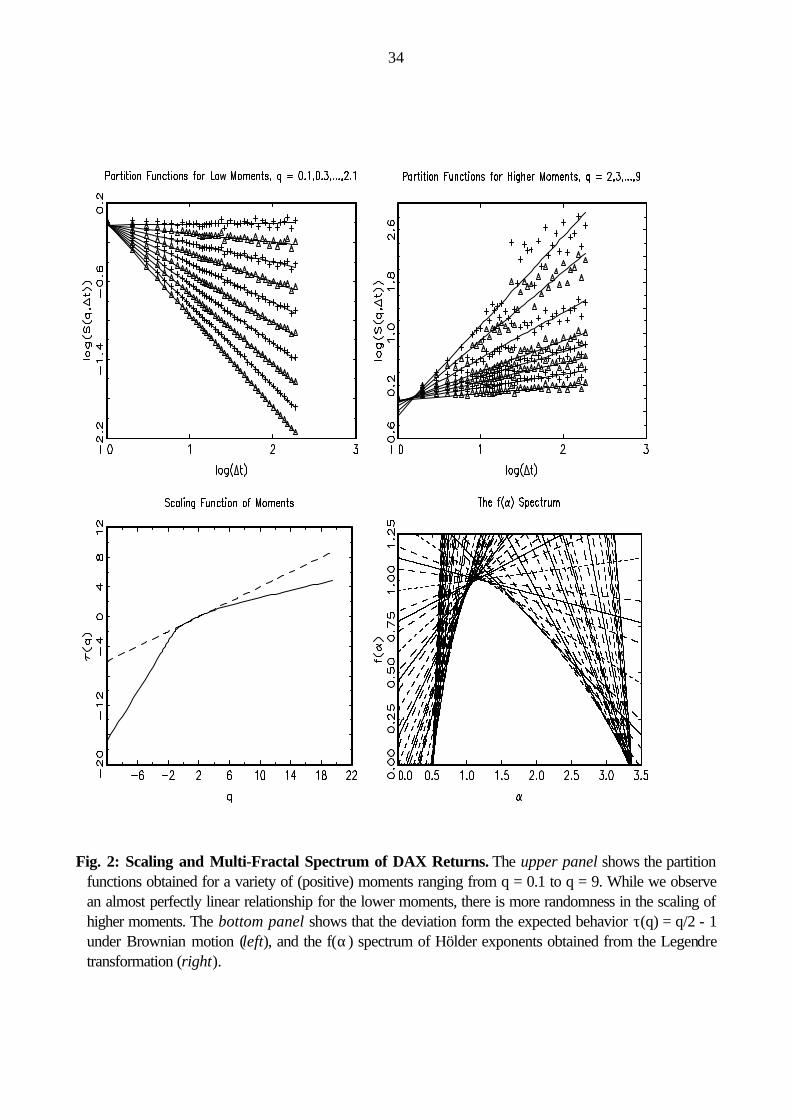
34

Fig. 2: Scaling and Multi-Fractal Spectrum of DAX Returns. The upper panel shows the partition

functions obtained for a variety of (positive) moments ranging from q = 0.1 to q = 9. While we observe an almost perfectly linear relationship for the lower moments, there is more randomness in the scaling of higher moments. The bottom panel shows that the deviation form the expected behavior τ(q) = q/2 - 1 under Brownian motion (left), and the f(α) spectrum of Hölder exponents obtained from the Legendre transformation (right).

35

Fig. 3: RMSE of f(αα ) and GMM estimators of the parameter λλ of the Lognormal multi-fractal

model. The shaded bars illustrate the development of the RMSE with sample size for the scaling

estimator, the unshaded bars illustrate that of the GMM estimator.

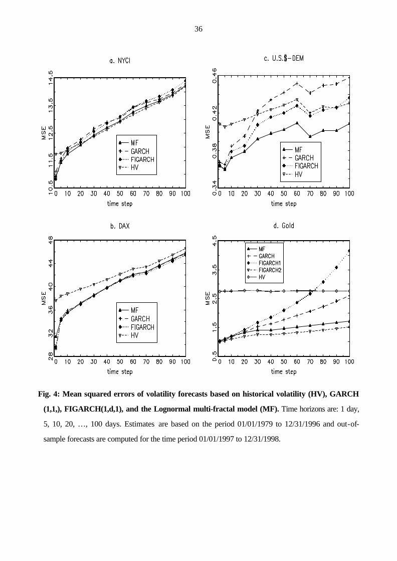
36

Fig. 4: Mean squared errors of volatility forecasts based on historical volatility (HV), GARCH

(1,1,), FIGARCH(1,d,1), and the Lognormal multi-fractal model (MF). Time horizons are: 1 day,

5, 10, 20, …, 100 days. Estimates are based on the period 01/01/1979 to 12/31/1996 and out-of-

sample forecasts are computed for the time period 01/01/1997 to 12/31/1998.