Embed Size (px)
Citation preview
The Mortality Transition, Malthusian Dynamics,and the Rise of Poor Mega-Cities∗
Remi Jedwab† and Dietrich Vollrath‡
January 2015
Abstract: The largest cities in the world today lie mainly in relatively poor countries, which
is a departure from historical experience, when the largest cities were typically found in
the richest places. Using new data on the demographic history of the 100 largest mega-
cities of today, we establish several new stylized facts distinguishing poor mega-cities from
historically rich mega-cities. To account for these facts we develop a model that combines
Malthusian models of endogenous population growth with urban models of agglomeration
and congestion, and it shows that the absolute growth of the urban population determines
whether a city becomes a poor or rich mega-city. We posit that poor mega-cities arose in
part because the post-war mortality transition raised their absolute growth above a crucial
threshold. Poor mega-cities continue to grow in size but not in living standards because
their poverty keeps population growth high. By expanding prior to the mortality transition,
historical mega-cities experienced smaller absolute growth that allowed them to sustain
wage growth and kept population growth relatively low.
Keywords: Urban Malthusianism; Demographic Regime; Megacities; Congestion; Growth
JEL classification: O11; O14; O18; L16; N10; N90; R10
∗We would like to thank Quamrul Ashraf, Alain Bertaud, Edward Glaeser, Stelios Michalopoulos, Paul Romer,Nico Voigtlaender, David Weil and seminar audiences at George Mason-George Washington Economic HistoryWorkshop, George Washington (IIEP and SAGE), George Washington University Urban Day, Harvard KennedySchool (NEUDC), Michigan, Minnesota (MIEDC), NYU Urbanization Project, Oxford (CSAE), Paris School ofEconomics (seminar and RSUE Workshop), University of California-Los Angeles (PACDEV), University Paris 1,U.S. Department of State (Strategic Consequences of Urbanization in Sub-Saharan Africa to 2025), WilliamsCollege, World Bank-George Washington University Conference on Urbanization and Poverty Reduction 2014,and World Bank-UNESCAP for very helpful comments. We thank the Institute for International Economic Policyat George Washington University for financial assistance.
†Remi Jedwab, Department of Economics, George Washington University, 2115 G Street, NW, Washington,DC 20052, USA (e-mail: [email protected]).
‡Corresponding Author: Dietrich Vollrath, Department of Economics, University of Houston, 201C McElhinneyHall, Houston, TX 77204, USA (e-mail: [email protected]).
1. INTRODUCTION
Urbanization has gone hand in hand with economic growth throughout history, and the
majority of world population now lives in cities. However, post-war developing countries
have urbanized in a fundamentally different manner compared to the historical experience
of currently developed countries. Specifically, the post-war period has seen the rise of poor
mega-cities in developing nations. Delhi, Dhaka, Karachi, Kinshasa, Lagos, and Manila are
some of the very largest urban agglomerations on the planet today, each with over 10 million
inhabitants. Only six of the currently largest 30 cities (London, Los Angeles, New York, Osaka,
Paris, and Tokyo) today are in high income countries. The prevalence of poor mega-cities
today runs counter to historical experience. In the first half of the 20th century, the very
largest urban agglomerations in the world were all in the most advanced economies.
The mega-cities of today’s developing world are also unlike their historical peers in that their
massive size is not indicative of rapid economic growth. This “poor country urbanization”
(Glaeser, 2013) has generated poor mega-cities that do not appear to be able to take advantage
of the agglomeration economies of their rich-country peers (World Bank, 2009).
Our aim in this paper is to provide an explanation for the rise of these poor mega-cities, and
why they differ from the historical experience of urbanization and rapid economic growth.
We propose that these mega-cities grew in poverty - and tend to remain mired in poverty -
because of what we characterize as urban Malthusian forces. To describe these forces, we build
a model that combines the insights of Malthusian models of endogenous population growth
(Ashraf & Galor, 2011; Galor & Weil, 2000) with the urban literature on equilibrium city
size (Henderson, 1974; Duranton & Puga, 2004; Duranton, 2013). The Malthusian literature
describes how limited resources will tend to reduce living standards as populations grows. The
urban literature captures the tension between the positive effects of agglomeration economies
and the negative effects of congestion to find that urban wages display an inverted-U shape
with respect to city population size. For a given set of urban technologies, in a sufficiently large
city the urban congestion effect dominates and generates a Malthusian relationship between
city size and city living standards.
In our model the growth rate of wages depends on the urban productivity growth rate relative
to the absolute change in the city population. A sufficiently large change in city population
can produce so much additional congestion that it offsets productivity growth, leaving wages
stagnant. Wage growth can be sustained in cities only if the absolute growth in city population
remains below a critical level, and this leads to two possible long-run equilibrium outcomes.
In the first, the absolute growth of cities is too large, and the economy ends up with poor
mega-cities. They end up in a bad cycle where low wages keep city population growth high,
and this keeps the absolute growth of the city so large that wages cannot grow. In contrast, the
second equilibrium occurs when a city has small absolute increases in population size, what
1
we call a historical mega-city. For these cities, low population growth allows for positive wage
growth, and this in turn leads to lower population growth rates, which further accelerates
wage growth. Both types of cities grow in population, but poor mega-cities grow because they
are poor, and rich mega-cities grow because they are rich.
We posit that a crucial distinction between poor mega-cities and their historical counterparts
is in their demographics. We collected historical data for today’s largest 100 mega-cities, from
antiquity to modern times, to document the differences in demographics between poor and rich
mega-cities. In modern developing nations nascent mega-cities experienced extremely large
absolute population growth, in large part because of the Mortality Transition of the 1940’s
and 1950’s. The rate of urban natural increase - the urban crude birth rate minus the urban
crude death rate - is well above those seen historically, and this is almost exclusively due to
the severe drop in urban crude death rates following the Mortality Transition. Cities in these
countries grew in absolute terms both because of in-migration from rural areas and significant
natural increase in the cities themselves. The combination put absolute city growth above the
critical threshold, and resulted in poor mega-cities.1
In comparison, historical cities grew prior to the Mortality Transition. The rate of urban
natural increase was low in historical cities because of high death rates. Even with in-
migration, the absolute growth in these city populations was relatively small and fell below the
critical threshold. Hence wage growth remained positive even as the cities expanded. When
significant declines in urban mortality rates did occur later in these cities, they were already
rich enough that population growth rates had slowed down and they were able to sustain wage
growth.
The main contribution of our paper is to explain the conditions under which these poor mega-
cities will arise, and to describe what their future may look like. In addition to this, our work
adds to the literature on the effects of demography on economic growth in general. Population
growth promotes economic growth if high population densities encourage human capital
accumulation or technological progress (Kremer, 1993; Becker, Glaeser & Murphy, 1999;
Lagerlof, 2003). In the urban setting we consider, there are positive impacts of population
growth due to agglomeration effects - but only over some range of population size. Population
growth also induces congestion effects, which negatively affects living standards, similar
to unified growth models that have a fixed resource (i.e. agricultural land) as part of the
production process (Galor & Weil, 1999, 2000; Strulik & Weisdorf, 2008; Galor, 2011). Our
work shows that the negative Malthusian effects need not arise because of natural resource
limits, but rather due to the nature of urbanization. Significantly, this implies that Malthusian
forces need not disappear as economies develop. Those forces remain operational even though
1Our paper is related to Jedwab, Christiaensen & Gindelsky (2014) who study the effects of urban naturalincrease on urbanization rates for developing countries from 1960-2010. While they focus their analysis on thegrowth of the urban population as a whole, we focus on the absolute growth of the largest cities of the world,across space and over time, and study how there are multiple equilibria in city size and city incomes.
2
agriculture and/or resource extraction cease to be significant sectors of production. The poor
mega-city equilibrium is one that arises perversely because of the success of interventions that
limited urban mortality rates while urban fertility remained relatively high. In this, our work
is similar to others that emphasize the negative effect of mortality interventions and/or the
positive impacts of mortality increases (Acemoglu & Johnson, 2007; Young, 2005).
This paper is close in subject matter to Voigtländer & Voth (2013a), who study the possibility
of multiple equilibria based on the urbanization process in historical Europe and China, but
do not consider the modern arrival of poor mega-cities in the developing world. In terms of
mechanisms, they introduce a non-linearity in mortality rates tied to a threshold urbanization
rate, and thus an exogenous shock like the Black Death allows Europe to move to a better
equilibrium. In comparison, our model introduces an explicit Malthusian force in city size,
and the equilibrium that a city ends up is not a result of an exogenous shock to city size, but
a change in the growth rate of city population.2
While there is some work on urbanization without growth (Fay & Opal, 2000), in general
there has been less attention given to poor mega-cities. See Duranton (2008), Henderson
(2010), and Duranton (2013) for recent surveys of cities in developing countries that do not
address the topic explicitly. In contrast, Glaeser (2013) begins with the same set of motivating
facts regarding poor mega-cities, but looks at them in a different light. His paper focuses on
the internal institutional structure that prevents mega-cities from reducing the overwhelming
congestion effects of their size, examining the trade-off between disorder and dictatorship.
His model does not consider the unique demographics leading to the origin of these mega-
cities.
The origin of poor mega-cities is certainly not mono-causal, and our explanation involving
Malthusian effects should be thought of as a complement to those involving changes in urban
transportation and housing technologies (i.e. the ability to build out or build up), changes in
preferences towards large cities, urban-biased policies, and others. Other explanations would
exacerbate the effects we are discussing here, but do not rule ours out.3
In the following section we document more fully the rise of poor mega-cities in the developing
world, and the underlying demographic features of these cities. Then, with those stylized facts
in place, we present our model of urban Malthusian dynamics, showing how an economy may
find itself in an equilibrium with poor mega-cities. We then compare this equilibrium to the
2Our work is also linked to studies that consider the effect of lower mortality on population and economicgrowth (Acemoglu & Johnson, 2007; Bleakley, 2007; Bleakley & Lange, 2009; Bleakley, 2010; Cutler et al.,2010) as well as those examining the effect of unexpected decreases in population on development (Young,2005; Voigtländer & Voth, 2009; Ashraf, Weil & Wilde, 2011; Voigtländer & Voth, 2013a,b). Relative to thoseworks we consider the implications of unexpected mortality changes from the perspective of cities and highlightsthat absolute changes in city populations are a crucial component of development.
3Notable alternatives include natural disasters (Barrios, Bertinelli & Strobl, 2006; Henderson, Storeygard &Deichmann, 2013), urban bias (Ades & Glaeser, 1995; Davis & Henderson, 2003; Henderson, 2003), and naturalresource exports (Gollin, Jedwab & Vollrath, 2015; Jedwab, 2013)
3
situation seen in historical European development and discuss the rise of poor mega-cities in
the context of our model.
2. RICH AND POOR MEGA-CITIES IN HISTORY
Table 1 shows the largest 30 cities in select years from 1700 to 2015 (Chandler, 1987; United
Nations, 2014). In 1700, the largest cities were all under 1 million persons in size, with
Istanbul, Tokyo, and Beijing all at around 700,000 inhabitants. While small in absolute size,
the largest cities in 1700 were generally located in the most economically advanced areas of
the world in that period. While London and Amsterdam had wages that were high relative
to the rest of the world, cities such as Istanbul, Tokyo, and Beijing all had wages equivalent
to those found in cities such as Paris and Naples (Allen, 2001; Allen et al., 2011; Özmucur &
Pamuk, 2002).
By 1900, the nature of the list of largest cities changed along several dimensions. First, the
absolute sizes were roughly ten times larger than in 1700. The largest city was London, with
6.5 million inhabitants, and there were 17 cities with over one million residents. Second, the
cities that dominate this list were the leading cities from the richest countries. London, New
York, Paris, Berlin, Chicago, Vienna, and Tokyo are all found on the list. Further down, we
see Birmingham, Boston, Hamburg, Liverpool, Manchester, and Philadelphia, all centers of
industrialization.
There were several large agglomerations of around 1 million in relatively poor places in 1900:
Beijing, Kolkata, Mumbai, and Rio de Janeiro. But none approached the absolute size of the
leaders like London or New York. Comparing 1900 to 1700, one can also see that their growth
in this period was not on the same scale as the richer cities. Beijing increased only from
700,000 to 1.1 million in the same 200 years that London went from 600,000 to 6.5 million.
Istanbul had 900,000 residents in 1900, up from 700,000 in 1700.
In 1950 the top cities remained those in relatively advanced nations but we see the very
beginnings of mega-city growth in relatively poor countries. Kolkata and Shanghai both had
more than four million inhabitants in 1950, putting them in the top 10 cities in the world
in 1950. Beijing, Cairo, Mexico City, Mumbai, and Rio de Janeiro were all over 2 million
inhabitants, reflecting rapid growth for most of them from earlier periods.
By 2015, the nature of the largest cities has changed dramatically. First, the absolute scale of
cities is 3-5 times larger than in 1950. Second, the composition of the list is now dominated
by cities in poor countries. Only Tokyo, Osaka, New York, Los Angeles, Paris, and London
are in what we would term rich countries. Instead we see cities such as Delhi, Mexico City,
Mumbai, and Sao Paulo. Countries that rank at the bottom in development levels have cities
present on this list, such as Dhaka (Bangladesh), Manila (Philippines), Karachi (Pakistan),
4
Lagos (Nigeria), and Kinshasa (DRC). Each of those poor cities have at least 11 million people,
making them larger in absolute size than nearly every city in the world in 1950.
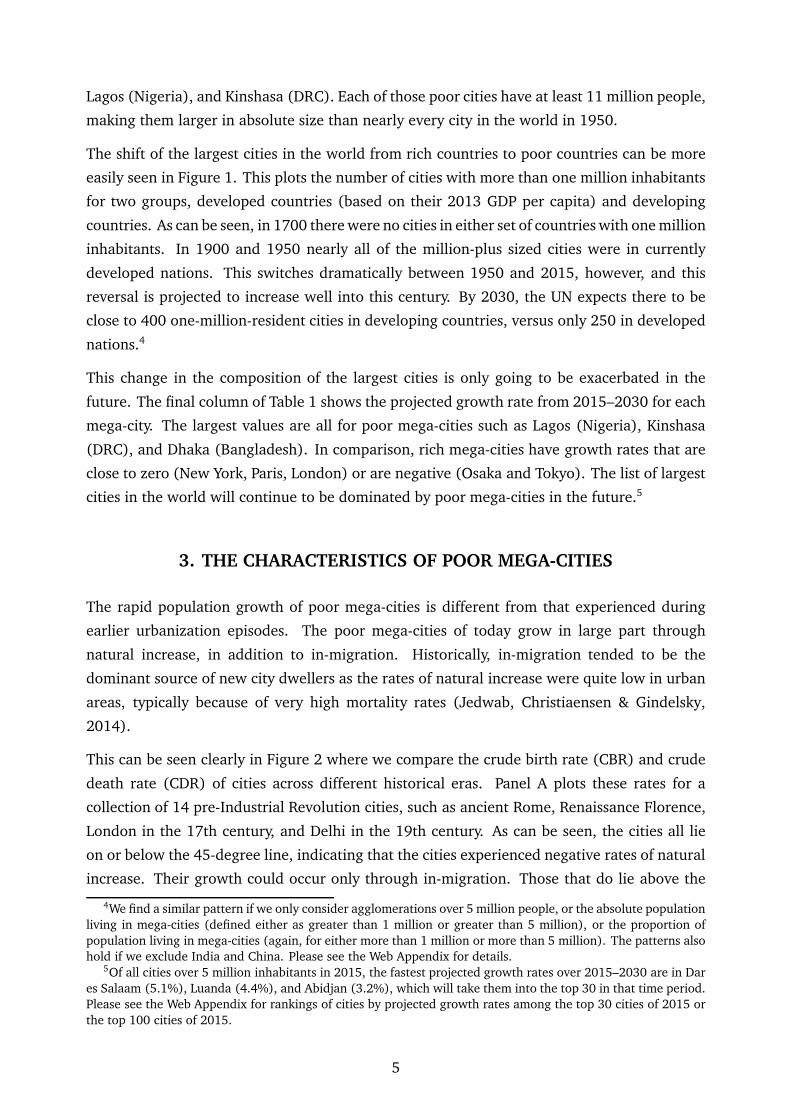
The shift of the largest cities in the world from rich countries to poor countries can be more
easily seen in Figure 1. This plots the number of cities with more than one million inhabitants
for two groups, developed countries (based on their 2013 GDP per capita) and developing
countries. As can be seen, in 1700 there were no cities in either set of countries with one million
inhabitants. In 1900 and 1950 nearly all of the million-plus sized cities were in currently
developed nations. This switches dramatically between 1950 and 2015, however, and this
reversal is projected to increase well into this century. By 2030, the UN expects there to be
close to 400 one-million-resident cities in developing countries, versus only 250 in developed
nations.4
This change in the composition of the largest cities is only going to be exacerbated in the
future. The final column of Table 1 shows the projected growth rate from 2015–2030 for each
mega-city. The largest values are all for poor mega-cities such as Lagos (Nigeria), Kinshasa
(DRC), and Dhaka (Bangladesh). In comparison, rich mega-cities have growth rates that are
close to zero (New York, Paris, London) or are negative (Osaka and Tokyo). The list of largest
cities in the world will continue to be dominated by poor mega-cities in the future.5
3. THE CHARACTERISTICS OF POOR MEGA-CITIES
The rapid population growth of poor mega-cities is different from that experienced during
earlier urbanization episodes. The poor mega-cities of today grow in large part through
natural increase, in addition to in-migration. Historically, in-migration tended to be the
dominant source of new city dwellers as the rates of natural increase were quite low in urban
areas, typically because of very high mortality rates (Jedwab, Christiaensen & Gindelsky,
2014).
This can be seen clearly in Figure 2 where we compare the crude birth rate (CBR) and crude
death rate (CDR) of cities across different historical eras. Panel A plots these rates for a
collection of 14 pre-Industrial Revolution cities, such as ancient Rome, Renaissance Florence,
London in the 17th century, and Delhi in the 19th century. As can be seen, the cities all lie
on or below the 45-degree line, indicating that the cities experienced negative rates of natural
increase. Their growth could occur only through in-migration. Those that do lie above the
4We find a similar pattern if we only consider agglomerations over 5 million people, or the absolute populationliving in mega-cities (defined either as greater than 1 million or greater than 5 million), or the proportion ofpopulation living in mega-cities (again, for either more than 1 million or more than 5 million). The patterns alsohold if we exclude India and China. Please see the Web Appendix for details.
5Of all cities over 5 million inhabitants in 2015, the fastest projected growth rates over 2015–2030 are in Dares Salaam (5.1%), Luanda (4.4%), and Abidjan (3.2%), which will take them into the top 30 in that time period.Please see the Web Appendix for rankings of cities by projected growth rates among the top 30 cities of 2015 orthe top 100 cities of 2015.
5
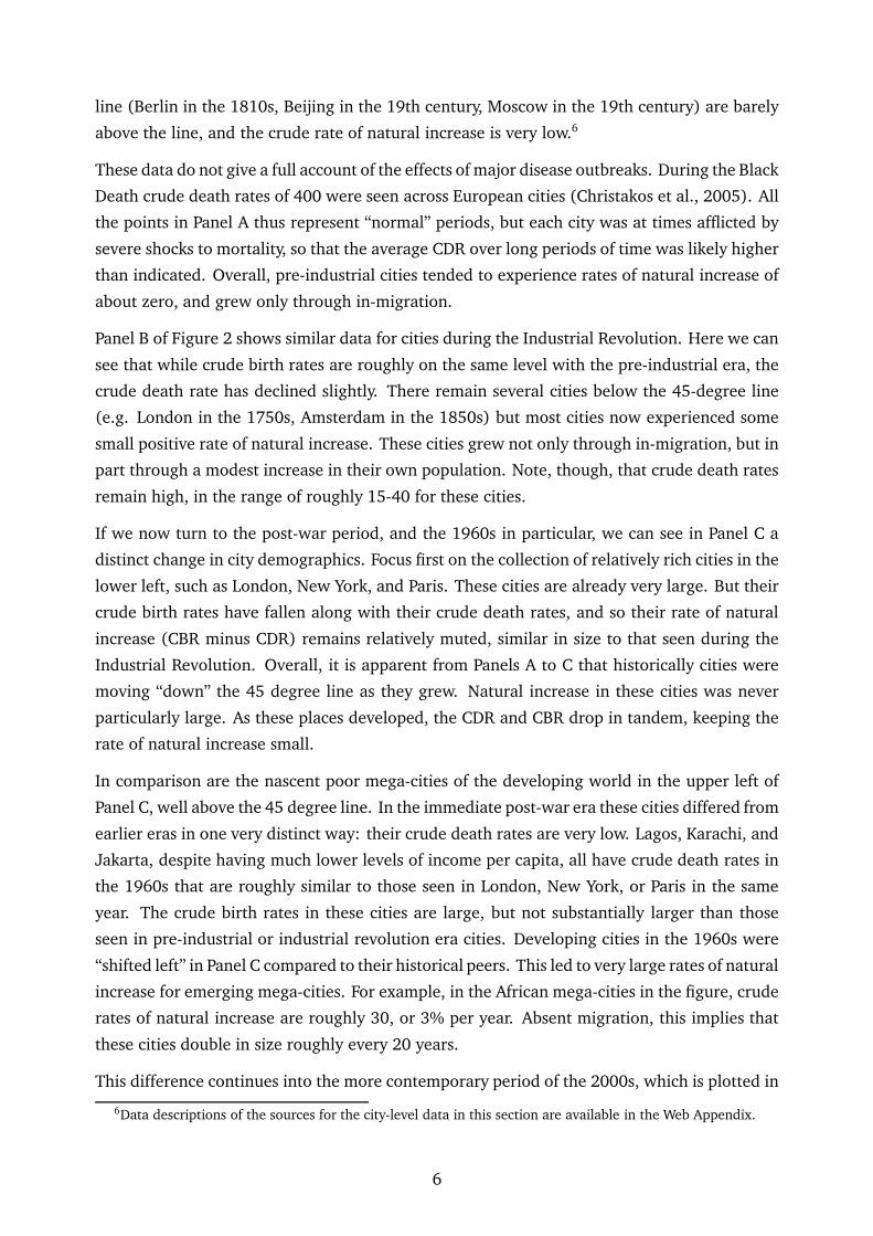
line (Berlin in the 1810s, Beijing in the 19th century, Moscow in the 19th century) are barely
above the line, and the crude rate of natural increase is very low.6
These data do not give a full account of the effects of major disease outbreaks. During the Black
Death crude death rates of 400 were seen across European cities (Christakos et al., 2005). All
the points in Panel A thus represent “normal” periods, but each city was at times afflicted by
severe shocks to mortality, so that the average CDR over long periods of time was likely higher
than indicated. Overall, pre-industrial cities tended to experience rates of natural increase of
about zero, and grew only through in-migration.
Panel B of Figure 2 shows similar data for cities during the Industrial Revolution. Here we can
see that while crude birth rates are roughly on the same level with the pre-industrial era, the
crude death rate has declined slightly. There remain several cities below the 45-degree line
(e.g. London in the 1750s, Amsterdam in the 1850s) but most cities now experienced some
small positive rate of natural increase. These cities grew not only through in-migration, but in
part through a modest increase in their own population. Note, though, that crude death rates
remain high, in the range of roughly 15-40 for these cities.
If we now turn to the post-war period, and the 1960s in particular, we can see in Panel C a
distinct change in city demographics. Focus first on the collection of relatively rich cities in the
lower left, such as London, New York, and Paris. These cities are already very large. But their
crude birth rates have fallen along with their crude death rates, and so their rate of natural
increase (CBR minus CDR) remains relatively muted, similar in size to that seen during the
Industrial Revolution. Overall, it is apparent from Panels A to C that historically cities were
moving “down” the 45 degree line as they grew. Natural increase in these cities was never
particularly large. As these places developed, the CDR and CBR drop in tandem, keeping the
rate of natural increase small.
In comparison are the nascent poor mega-cities of the developing world in the upper left of
Panel C, well above the 45 degree line. In the immediate post-war era these cities differed from
earlier eras in one very distinct way: their crude death rates are very low. Lagos, Karachi, and
Jakarta, despite having much lower levels of income per capita, all have crude death rates in
the 1960s that are roughly similar to those seen in London, New York, or Paris in the same
year. The crude birth rates in these cities are large, but not substantially larger than those
seen in pre-industrial or industrial revolution era cities. Developing cities in the 1960s were
“shifted left” in Panel C compared to their historical peers. This led to very large rates of natural
increase for emerging mega-cities. For example, in the African mega-cities in the figure, crude
rates of natural increase are roughly 30, or 3% per year. Absent migration, this implies that
these cities double in size roughly every 20 years.
This difference continues into the more contemporary period of the 2000s, which is plotted in
6Data descriptions of the sources for the city-level data in this section are available in the Web Appendix.
6
Panel D of Figure 2. Rich mega-cities such as London, New York, and Paris remain in roughly
the same position as in the 1960s, with low crude death and crude birth rates. The poor mega-
cities of the developing world have also shifted down to lower crude birth rates. However, the
crude death rates in these poor mega-cities are much lower than the historical comparisons, for
the most part falling below 10 per thousand. Thus in the 2000s poor mega-cities continued to
have extremely rapid rates of natural increase. A notable exception are Chinese cities, which
in the 1960s (Panel C) looked quite similar to other developing mega-cities, but after the
introduction of the one-child policy moved in the 2000s (Panel D) to a pattern of crude death
and crude birth rates very similar to rich mega-cities.
The deviation of the developing countries in Panels C and D from the historical norms
appears due, in large part, to what Acemoglu & Johnson (2007) refer to as the international
epidemiological transition. Following 1940, there was a rapid improvement in health
(particularly in infant mortality) in many developing countries. This was due to the availability
of vaccines and new treatments (e.g. antibiotics), a world-wide effort by the World Health
Organization and others to provide access to those vaccines and new treatments, and a focus
on rapid dissemination of public health innovations to developing countries (Stolnitz, 1955;
Davis, 1956; Preston, 1975).7
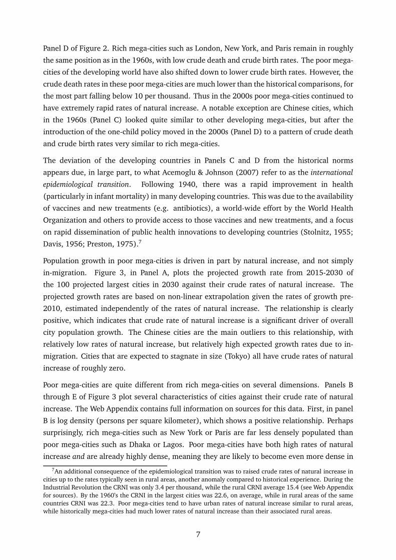
Population growth in poor mega-cities is driven in part by natural increase, and not simply
in-migration. Figure 3, in Panel A, plots the projected growth rate from 2015-2030 of
the 100 projected largest cities in 2030 against their crude rates of natural increase. The
projected growth rates are based on non-linear extrapolation given the rates of growth pre-
2010, estimated independently of the rates of natural increase. The relationship is clearly
positive, which indicates that crude rate of natural increase is a significant driver of overall
city population growth. The Chinese cities are the main outliers to this relationship, with
relatively low rates of natural increase, but relatively high expected growth rates due to in-
migration. Cities that are expected to stagnate in size (Tokyo) all have crude rates of natural
increase of roughly zero.
Poor mega-cities are quite different from rich mega-cities on several dimensions. Panels B
through E of Figure 3 plot several characteristics of cities against their crude rate of natural
increase. The Web Appendix contains full information on sources for this data. First, in panel
B is log density (persons per square kilometer), which shows a positive relationship. Perhaps
surprisingly, rich mega-cities such as New York or Paris are far less densely populated than
poor mega-cities such as Dhaka or Lagos. Poor mega-cities have both high rates of natural
increase and are already highly dense, meaning they are likely to become even more dense in
7An additional consequence of the epidemiological transition was to raised crude rates of natural increase incities up to the rates typically seen in rural areas, another anomaly compared to historical experience. During theIndustrial Revolution the CRNI was only 3.4 per thousand, while the rural CRNI average 15.4 (see Web Appendixfor sources). By the 1960’s the CRNI in the largest cities was 22.6, on average, while in rural areas of the samecountries CRNI was 22.3. Poor mega-cities tend to have urban rates of natural increase similar to rural areas,while historically mega-cities had much lower rates of natural increase than their associated rural areas.
7
the future.
This density is indicative of congestion rather than positive agglomeration effects. Panel C
shows that slum shares (measured at the national level) are much higher in poor mega-cities
than in rich ones. Roughly two-thirds of the residents of Dhaka, Lagos, and Kinshasa live in
slums, which is measured based on lack of access to services like running water or sewage.
Density and slum shares are not the only means of measuring congestion. The Web Appendix
contains supplemental plots using a variety of alternative measures of congestion. Poor mega-
cities with rapid population growth perform worse on each metric.
The high rates of natural increase and density of poor mega-cities do not necessarily indicate
a large supply of skilled workers, which may generate positive agglomeration effects. Panel D
shows the dependency ratio (the share of those under 14 and 65-plus to population aged 15-
64) across our sample of cities. In poor mega-cities with high crude rates of natural increase,
this dependency ratio reaches more than 60 percent. While there are several richer cities
with relatively high values (Tokyo or Osaka) due to large elderly populations, in general the
dependency ratio is lower the smaller the crude rate of natural increase. Poor mega-cities
grow quickly through natural increase, but this does not necessarily lead to rapid growth in
the effective labor force.8
Further, the labor force that does exist in poor mega-cities tends to be low skilled. Panel E
plots the tertiary school completion rate against the crude rate of natural increase. In poor
mega-cities, the share of college-educated workers is close to zero, as compared to rich mega-
cities like London, New York, or Paris where it is one-third or more. Poor mega-cities have
large populations, but due to age structure and lack of education, this does not translate to a
large effective workforce.
This is consistent with the final Panel F of figure 3, where we show that city crude rates of
natural increase correlate negatively with income levels in 2000. As we do not have individual
city-level data, we plot city crude rates of natural increase against country-level GDP per capita.
Natural increase is extremely high in the African and Asian mega-cities located in the poorest
countries (e.g. Dhaka, Kinshasa, and others). Natural increase falls regularly as countries get
richer, consistent with their rising education levels seen in panel E.9
Overall, it is the distinct characteristics of developing countries seen in both figures 2 and 3,
in our model, the source of their move into a poor mega-city equilibrium. The rapid rate of
natural increase in these cities has two effects. First, it implies that they very quickly hit the
Malthusian congestion effects in urban areas: high density, a large prevalence of slums, low
education, and high dependency ratios. Second, the high rate of natural increase lowers living
8The Web Appendix contains alternative plots using child dependency and old-age dependency, each showinghigher dependency ratios in poor mega-cities with only a few exceptions.
9The Web Appendix contains further plots of city labor force characteristics on education, employment,productivity, and poverty that are consistent with the relationships in panels E and F.
8
standards due to that congestion. Rapid natural increase thus keeps wages low, which in turn
implies that natural increase remains high, and the poor mega-cities remain stuck in a low-
wage equilibrium where they grow without bound. The demographic shock of low mortality
rates in the post-war era seen in figure 2, by increasing the rate of natural increase, contributed
to the arrival and persistence of the poor mega-city equilibrium.
4. A MODEL OF RICH AND POOR MEGA-CITIES
The facts presented above established that poor mega-cities have distinctly different
demographic patterns than mega-cities of the past. One reaction is that these demographic
patterns, while deviating from past experience, are just part of a transitory phase of growth
in these cities, and that they will become rich mega-cities given sufficient time. What we will
show in the model that follows is that this is likely too optimistic an outlook. Under reasonable
assumptions that match the facts we outlined in the prior sections, we show that a poor mega-
city equilibrium exists. In particular, cities that experience extremely rapid absolute gains in
population can find themselves stuck in an equilibrium with low wages and high population
growth. As we discuss after the model is presented, the Mortality Transition after World War
II may have pushed cities into the poor mega-city equilibrium.
Our model is based on two strands of literature. First, we adopt explicit micro-foundations for
city production that display both agglomeration and congestion, as emphasized in the urban
economics literature. Second, we combine that with endogenous population growth as in a
typical quantity/quality trade-off model. The combination shows that it is the absolute growth
in city population, not the growth rate, that is crucial in determining whether a city ends up a
poor or a rich mega-city.
We derive the model for a mega-city that has an associated rural area which provides a possible
pool of migrants. The absolute growth of the city population will depend on the natural
increase in both the urban and rural sectors, as well as on the urbanization rate, which we will
initially take as exogenously given. We show in the Web Appendix how to adapt the model
to allow for a distribution of cities and/or an endogenous determination of the urbanization
rate. The basic logic of the single city model will not be altered by the introduction of either
element. For clarity we therefore continue to work with the single city model.
4.1 The City Sector
The city in our model will benefit from agglomeration effects in the sense that output
has increasing returns to scale with respect to city population. This arises in a model of
differentiated inputs to city production combined with firm fixed costs. As the scale of the city
increases, more firms find they can make enough profits to offset the fixed cost, the number
9
of intermediate goods in production rises, and this increases output.10
4.1.1 Production and Agglomeration
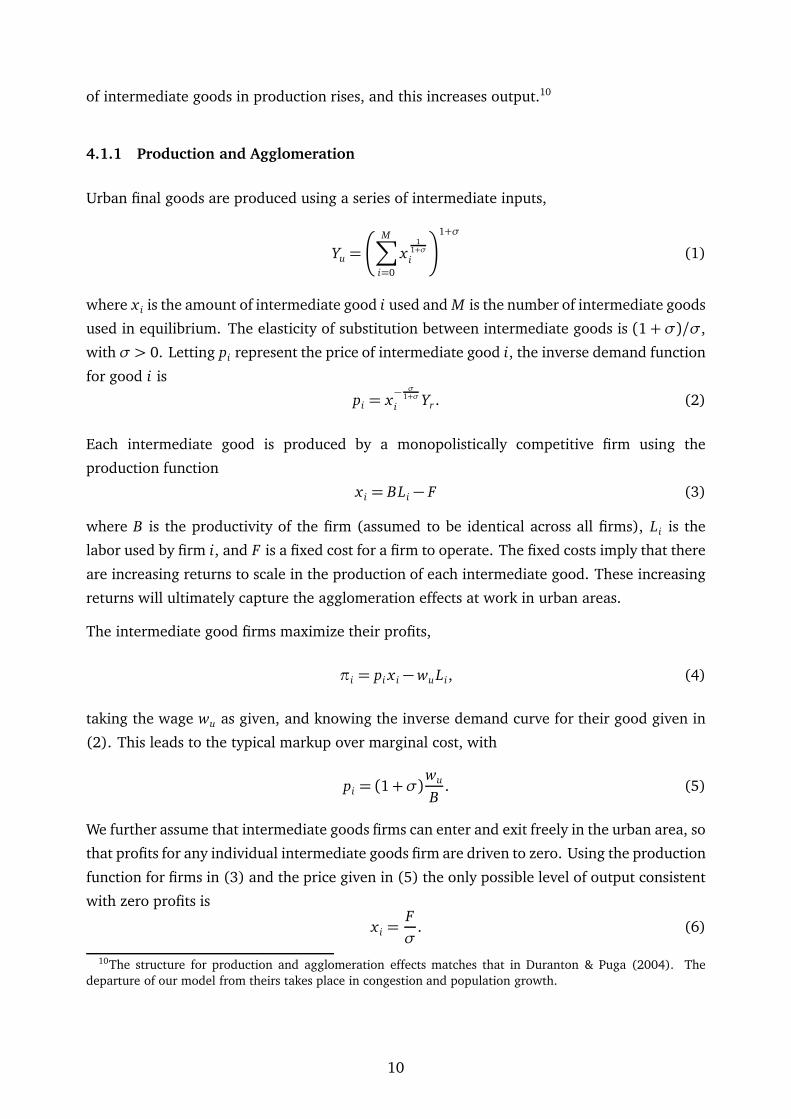
Urban final goods are produced using a series of intermediate inputs,
Yu =
M∑
i=0
x1
1+σ
i
1+σ
(1)
where x i is the amount of intermediate good i used and M is the number of intermediate goods
used in equilibrium. The elasticity of substitution between intermediate goods is (1+σ)/σ,
withσ > 0. Letting pi represent the price of intermediate good i, the inverse demand function
for good i is
pi = x−σ
1+σ
iYr . (2)
Each intermediate good is produced by a monopolistically competitive firm using the
production function
x i = BLi − F (3)
where B is the productivity of the firm (assumed to be identical across all firms), Li is the
labor used by firm i, and F is a fixed cost for a firm to operate. The fixed costs imply that there
are increasing returns to scale in the production of each intermediate good. These increasing
returns will ultimately capture the agglomeration effects at work in urban areas.
The intermediate good firms maximize their profits,
πi = pi x i −wu Li, (4)
taking the wage wu as given, and knowing the inverse demand curve for their good given in
(2). This leads to the typical markup over marginal cost, with
pi = (1+σ)wu
B. (5)
We further assume that intermediate goods firms can enter and exit freely in the urban area, so
that profits for any individual intermediate goods firm are driven to zero. Using the production
function for firms in (3) and the price given in (5) the only possible level of output consistent
with zero profits is
x i =F
σ. (6)
10The structure for production and agglomeration effects matches that in Duranton & Puga (2004). Thedeparture of our model from theirs takes place in congestion and population growth.
10
Given this level of output, each firm hires
Li =1+σ
σ
F
B. (7)
As each intermediate good provider is identical, their total demand for labor must equal the
total supply of labor in the urban area, Lu
M∑
i=0
Li = Lu, (8)
which can be solved for the equilibrium number of firms,
M =Lu
Li
=σ
1+σ
B
FLu. (9)
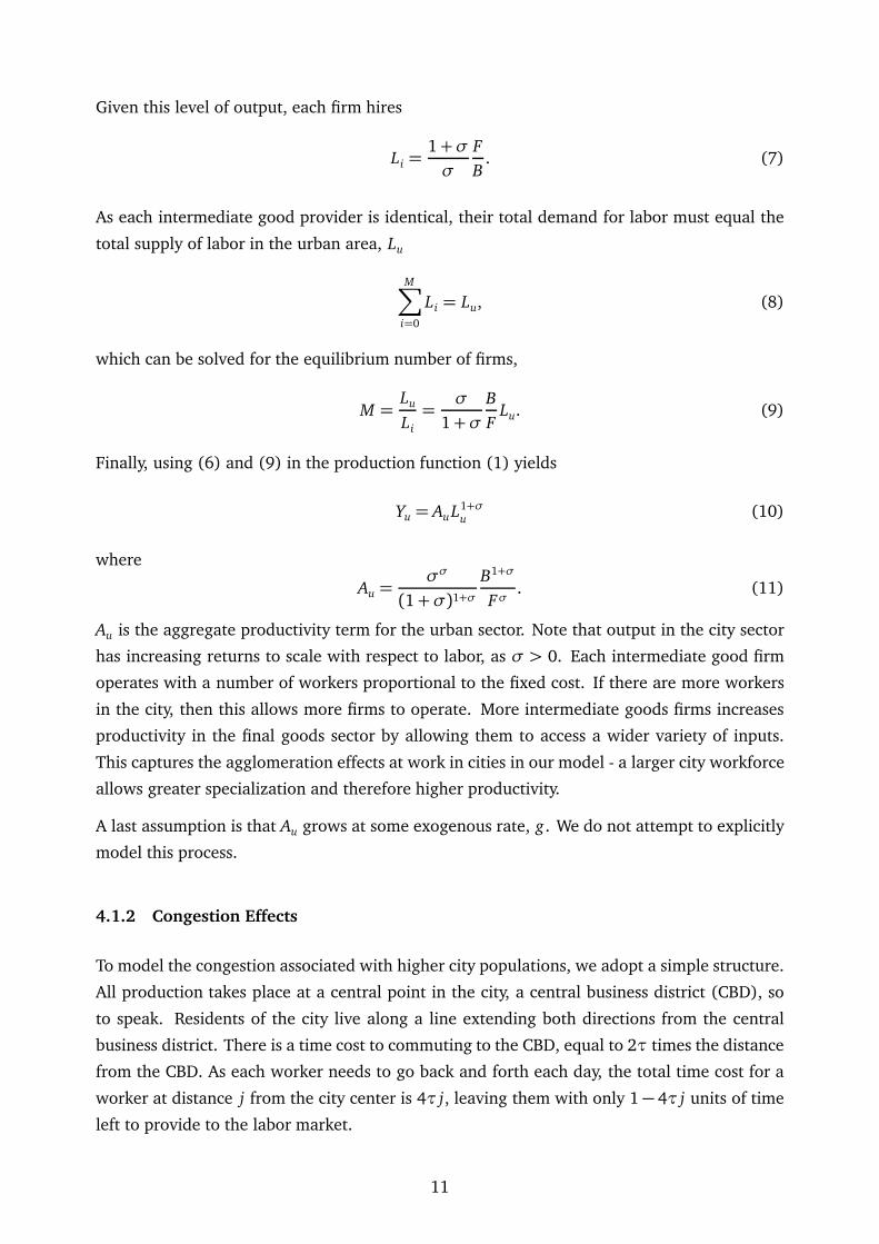
Finally, using (6) and (9) in the production function (1) yields
Yu = AuL1+σu
(10)
where
Au =σσ
(1+σ)1+σB1+σ
Fσ. (11)
Au is the aggregate productivity term for the urban sector. Note that output in the city sector
has increasing returns to scale with respect to labor, as σ > 0. Each intermediate good firm
operates with a number of workers proportional to the fixed cost. If there are more workers
in the city, then this allows more firms to operate. More intermediate goods firms increases
productivity in the final goods sector by allowing them to access a wider variety of inputs.
This captures the agglomeration effects at work in cities in our model - a larger city workforce
allows greater specialization and therefore higher productivity.
A last assumption is that Au grows at some exogenous rate, g. We do not attempt to explicitly
model this process.
4.1.2 Congestion Effects
To model the congestion associated with higher city populations, we adopt a simple structure.
All production takes place at a central point in the city, a central business district (CBD), so
to speak. Residents of the city live along a line extending both directions from the central
business district. There is a time cost to commuting to the CBD, equal to 2τ times the distance
from the CBD. As each worker needs to go back and forth each day, the total time cost for a
worker at distance j from the city center is 4τ j, leaving them with only 1− 4τ j units of time
left to provide to the labor market.
11
The distance that each worker has to travel is a function of the number of workers in the city,
Nu. Each worker uses up one unit along the line, so that the maximum distance a worker is
from the center is Nu/2, as workers can live in either direction. Integrating over all the workers
we can find the total labor supply
Lu = 2
∫ Nu/2
0
(1− 4τ j) d j = Nu [1−τNu] . (12)
Here we can see the impact of congestion. Labor supply, Lu is increasing in the number of
city workers, Nu, but only up to a point. Eventually increased city population becomes so
burdensome that the actual labor supplied by workers falls.
The effective labor force in (12) has a strict upper limit of Nu = 1/τ. Above that limit the
labor provided is zero, and this would put a firm cap on city size. To avoid this limit, we make
a functional modification to this standard model of city congestion. We let τ be a function of
city size itself, specifically setting τ = (1 − ex p(−λNu))/Nu. λ captures the speed at which
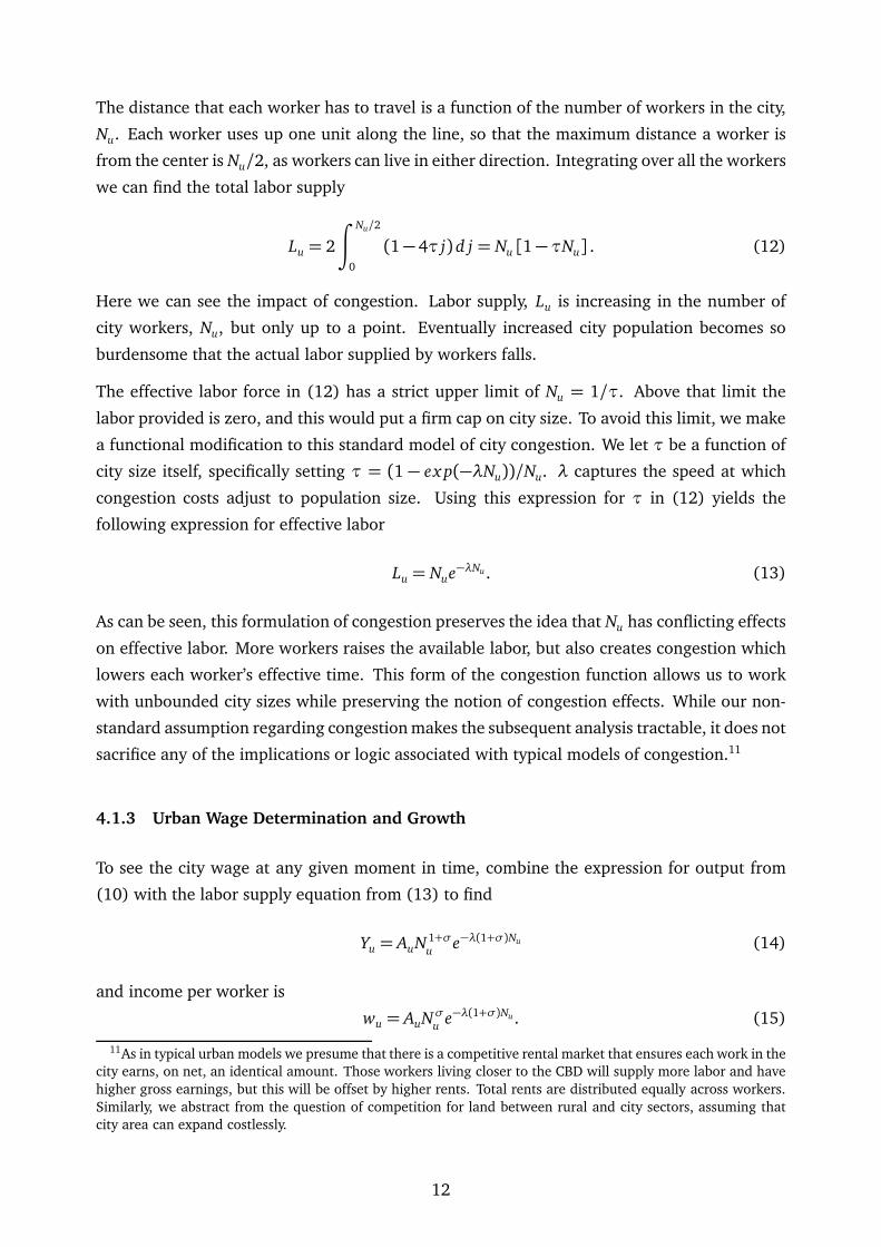
congestion costs adjust to population size. Using this expression for τ in (12) yields the
following expression for effective labor
Lu = Nue−λNu. (13)
As can be seen, this formulation of congestion preserves the idea that Nu has conflicting effects
on effective labor. More workers raises the available labor, but also creates congestion which
lowers each worker’s effective time. This form of the congestion function allows us to work
with unbounded city sizes while preserving the notion of congestion effects. While our non-
standard assumption regarding congestion makes the subsequent analysis tractable, it does not
sacrifice any of the implications or logic associated with typical models of congestion.11
4.1.3 Urban Wage Determination and Growth
To see the city wage at any given moment in time, combine the expression for output from
(10) with the labor supply equation from (13) to find
Yu = AuN 1+σu
e−λ(1+σ)Nu (14)
and income per worker is
wu = AuNσu
e−λ(1+σ)Nu. (15)
11As in typical urban models we presume that there is a competitive rental market that ensures each work in thecity earns, on net, an identical amount. Those workers living closer to the CBD will supply more labor and havehigher gross earnings, but this will be offset by higher rents. Total rents are distributed equally across workers.Similarly, we abstract from the question of competition for land between rural and city sectors, assuming thatcity area can expand costlessly.
12
What can be seen here is that the number of city workers, Nu, influences earnings in the
city, and that these earnings form an inverted U-shape. That is, for low levels of Nu earnings
are increasing in city workers as the agglomeration effects outweigh the congestion effect.
Eventually, though, when Nu is large enough the congestion effects dominate and more
city workers will lower earnings. Differentiating (15) with respect to Nu shows the wage-
maximizing number of workers is N ∗ = σ/[(1 + σ)λ]. Above that level, wages fall as more
residents arrive in the city.
wu
wu
= g +Nu
Nu
[σ−λ(1+σ)Nu] (16)
so that we have the growth rate of population times this term in the brackets. The term in
brackets captures agglomeration (σ) and congestion (λ(1+σ)Nu). As the absolute size of Nu
goes up, congestion gets worse.
Given this determination of the wage, we can turn to how this wage will grow (or stagnate).
Taking logs and time derivatives, we have that
wu
wu
= g +σNu
Nu
−λ(1+σ)Nu (17)
where recall that g is the exogenous growth rate of Au. City wage growth depends positively
on productivity growth, and on the agglomeration effects coming from the growth rate of the
city population.12
But there are congestion effects, and the last term in (17) captures this drag on wages. Notice
that the congestion term depends on the absolute change in city population, not its growth
rate. Larger absolute increases in city population push up congestion costs for all existing
residents, no matter how many there are, and this lowers the wage.
From equation (17) we can already develop the basic intuition behind poor mega-cities, and
the relevance of the Mortality Transition coming before widespread urbanization. In poor
countries, the Mortality Transition raised the rate of urban natural increase, so that even
without any in-migration from rural areas, cities experienced very large absolute gains in
population. Urbanization then pushes even more workers into cities from rural areas, and
together this leads to very large absolute gains in city population, Nu. If this absolute gain is
too large, then wage growth can actually become negative, leading to a poor mega-city. This
poverty, as we will discuss in more detail below, keeps population growth rates high, and thus
the poor mega-city becomes self-perpetuating.
12The dependence of wage growth on the absolute growth in urban population is not an artifact of our particularassumption regarding congestion. This would appear in any model where the absolute number of residents wasassociated with higher congestion costs. It implies that a city doubling in size from 50 thousand to 100 thousandresidents will be able to sustain higher wage growth than one doubling from 500 thousand to 1 million, ceterisparibus.
13
Urbanizing before the Mortality Transition, as in currently rich mega-cities, avoided this
problem. With high mortality, and particularly with high mortality in urban areas, the absolute
increase in city populations was very small over time. Even with in-migration from rural areas,
Nu was small, and this ensured that wage growth could remain positive. As wages rose, this
induced lower population growth rates, which reinforces the outcome of positive wage growth
in cities.
A simple example of the difference is between New York and Dhaka. Both have roughly 18
million inhabitants today, but the absolute growth in city population was much slower in New
York. In the 19th century New York grew by about 67,000 residents per year, and at its peak
from 1900 to 1940 grew at roughly 155,000 per year. In contrast between 1960–2010 Dhaka
grew by about 284,000 per year, reaching 445,000 per year in the 2000’s. The absolute growth
of modern developing cities is on a different scale than that experienced historically.
4.2 City Population Growth
Wage growth in the city sector depends on both the growth rate of the city population as well
as its absolute change. By modeling the population growth process more formally, we can
better understand the conditions under which poor mega-cities will develop. City population
growth depends on both the urban rate of natural increase and on in-migration from rural
areas, so we will need models of population processes in both sectors.
In each sector, there is natural increase in population. We model this natural increase as
depending on the wage rate, w(t), as well as a sector-specific mortality shifter, m. Specifically,
we have
N N Iu= φ(w(t), mu) (18)
N N Ir= φ(w(t), mr),
where φ(w(t), mi) is the function describing the relationship of natural increase to wages
and the shifter, with i ∈ (u, r). The φ() function captures demographic behavior related to
income, including both fertility and mortality responses, and the shifter mi is intended to
capture exogenous changes in the underlying mortality regime.
We do not specify precise micro-foundations for theφ() function, as those are readily available
14
from the literature.13 The specific properties that we assume are as follows,
φw(w(t), mi) < 0 (19)
φm(w(t), mi) < 0 (20)
limw→∞
φ(w(t), mi) = φmin. (21)
The first property simply states that natural increase in either sector is decreasing with
income, matching the empirical evidence.14 The second property states that natural increase
is negatively related to exogenous mortality, mi. We think of mi as representing level effects
on population growth. In particular, the mortality transition will be captured by a decrease in
mi. The final property says that regardless of sector, as wages get arbitrary high, the rate of
natural increase reaches a minimum. This minimum need not be zero.
With total population equalling the sum of urban and rural population, N(t) = Nu(t)+Nr(t),
the absolute change in total population is the sum of natural increase in the two sectors,
N = Nu(t)NN Iu+ Nr(t)N
N Ir
. (22)
Plugging in (19) for the natural increase terms, dividing by N , and suppressing the time
notation we haveN
N=
Nu
Nφ(w, mu) +
Nr
Nφ(w, mr), (23)
as the expression for total population growth.
Define the urbanization rate (again suppressing time notation) as
u =Nu
N. (24)
It follows that the growth rate of the urban population is simply
Nu
Nu
=u
u+
N
N. (25)
Use expression (23) to plug in for the growth rate of total population and after a small amount
of manipulation we have that the growth rate of city population can be written as
Nu
Nu
= φ(w, mu) +u
u+ (1− u) [φ(w, mr)−φ(w, mu)] . (26)
13Jones, Schoonbroodt & Tertilt (2010) and Galor (2011) provide reviews of common explanations for therelationship between wages, fertility, and mortality.
14Becker (1960) observed the negative relationship of incomes and fertility, and see Jones, Schoonbroodt &Tertilt (2010) for a more recent summary of the available evidence. Allowing for a positive effect of income onpopulation growth at very low income levels, as in unified growth models (Galor, 2011), complicates the analysisbut does not change the ultimate implications of the model.
15
The first term on the right is urban natural increase, i.e. the growth in city population arising
solely from the growth of urban families, and ignoring in-migration. The last two terms on
the right capture net migration. If u/u > 0, and the urbanization rate is rising, then this
implies a net movement of population from rural areas to the city. Additionally, if there is
some difference in natural increase between rural and urban areas (φ(w, mr) − φ(w, mu)),
then there will be additional net migration between the two. Historically economies had
φ(w, mr) > φ(w, mu) because of high city mortality (i.e. a high value of mu), and even with a
fixed urbanization rate this led to a constant flow of workers from rural areas to the city.15
From equation (26) we can identify several of the important forces that will determine whether
an economy ends up with poor mega-cities or rich ones. First, note that the growth rate of
city population, and by extension the absolute change in city population, depends on the rate
of natural increase in cities. The mortality transition, by raising φ(w, mu), raises absolute city
population growth, and hence lowers the growth rate of wages. Lower wages implies that
natural increase remains high, and hence city population growth remains high.
For clarity, we will continue by analyzing an economy where the urbanization rate, u, is
constant, and hence u/u = 0. Available in the appendix is a discussion of the model with
the urbanization rate allowed to change over time. With u = 0, we then define the following
function,
n(w, cu) ≡ φ(w, mu) + (1− u) [φ(w, mr)−φ(w, mu)] (27)
as the instantaneous growth rate of city population. It is straightforward to see that n(w, mu)
inherits the properties of the φ(w, mu) function and therefore
nw(w, mu) < 0 (28)
nm(w, mu) < 0 (29)
limw→∞
n(w, cu) = nmin. (30)
The growth rate of city population is negatively related to wages, as this lowers population
growth in both rural and urban sectors. City population growth is also negatively related to the
value of mu. As wages rise, the growth rate falls towards a minimum, and again this minimum
need not equal zero.
4.3 Equilibrium Outcomes
We can now characterize the dynamics of wages with respect to city population size. From
equation (17) we know that growth in wages is positive if productivity growth and the
15An additional consideration is that in many developing countries after the mortality transition, cities becameless deadly than rural areas, and φ(w, mr) < φ(w, mu). This would, by itself, limit city population growth. Butthen any increase in urbanization, u, actually increased city population growth as more people moved into alow-mortality area, further raising population growth.
16
agglomeration effects are large relative to the congestion effect driven by the absolute change
in city population. Given that city population growth itself depends on the wage we will be
able to define a relationship between the wage rate and city population size that determines
whether wages grow or not. Following that we will provide the conditions under which a city
will be able to sustain positive wage growth over time.
In words, a city will be able to sustain wage growth indefinitely if their rate of absolute
population growth is sufficiently small. This will occur if either their initial wage is high,
and so natural increase is low, or if their initial size is small, and hence the absolute growth
in city size is also small. Rich mega-cities will arise because their wages grow fast enough
to lower population growth rates, which in turn reinforces wage growth. Poor mega-cities
will arise because their population growth makes wages growth slow enough (or shrink) to
keep population growth high, which in turn reinforces the slow or falling wage growth. We
then show that a sufficiently large boost to population growth, such as occurred following the
mortality transition, could push a city into the poor mega-city equilibrium regardless of initial
conditions. Conversely, a sufficiently large drop in population growth, such as with China’s
single-child policy, could push a city into the rich mega-city equilibrium.
More formally, we begin by establishing the conditions under which wage growth in urban
areas will be positive.
Lemma 1. There is a function
N(w, mu) ≡g
λ(1+σ)n(w, mu)+
σ
λ(1+σ)(31)
such that
• For Nu < N (w, mu), wage growth is positive, w/w > 0
• For Nu > N (w, mu), wage growth is negative, w/w < 0.
and with the properties
• ∂ N (w, mu)/∂ w > 0
• ∂ N (w, mu)/∂mu > 0.
Proof. Please see appendix.
If the city population is sufficiently small, then the absolute growth in city population is also
small enough that congestion effects do not overwhelm the positive effects of agglomeration
and productivity growth, and wages grow. N (w, mu) defines the cutoff level for city population
to achieve this wage growth.
The cutoff is increasing with the wage. This occurs because at higher wages, the city population
growth rate is smaller, given the properties of n(w, mu). With a smaller growth rate, the
absolute change in city population is small even in a large city, and the congestion effects
17
do not offset productivity growth. Hence, at higher wages the absolute size of the city can
be larger and yet still have positive wage growth. Whether cities can maintain positive wage
growth over time is the subject of the following lemma.
Lemma 2. There is a function
N (w, mu) ≡ N(w, mu)1
1+Ω, (32)
where Ω= −n(w, mu)2/nw(w, mu)wg > 0 such that
• If Nu < N(w, mu), then Nu < N(w, mu)
• If Nu > N(w, mu), then Nu > N(w, mu)
and with the properties that
• N(w, mu) < N (w, mu)
• N(w, mu)→ 0 as w→ 0
• N(w, mu)→ N(w, mu) as w→∞
Proof. Please see appendix.
Lemma 2 shows that for cities below a lower threshold, N (w, mu), wage growth will be positive
and their population growth is low enough to continue to stay below N(w, mu). But can those
cities indefinitely maintain wage growth as their populations grow? Or will they eventually
become so big that congestion effects overwhelm the growth in productivity? What the
following Proposition establishes is that if city size is smaller than N(w, mu) to begin with, then
in fact it will always remain below that threshold and wage growth will be positive forever.
These cities become rich mega-cities. Conversely, cities with populations above the threshold
N(w, mu)will grow in size too quickly and eventually reach a point where congestion overtakes
them. These become poor mega-cities.
Proposition 1. Given initial conditions w(0) and Nu(0) there are two possible equilibrium
outcomes
(a) Poor Mega-City: If Nu(0) ≥ N (w(0), mu) then wages will approach zero, limt→∞w(t) = 0,
and population growth will remain strictly above nmin.
(b) Rich Mega-City: If Nu(0) < N (w(0), mu) then wage growth is always positive, w/w > 0∀t,
and population growth approaches the minimum nmin.
Proof. Please see appendix.
The intuition for rich mega-cities in Proposition 1 is that for a sufficiently small city wage
growth is rapid enough that the city population growth rate shrinks relatively quickly. As
the population growth rate falls, the absolute change in city size is never sufficient to have
congestion effects overwhelm productivity growth, and hence wages continue to rise. As
18
population growth is decreasing in wages, once started, this process reinforces itself as time
goes on. Note that population growth goes to nmin, which can be non-zero, meaning that both
wages and city size can continue to grow indefinitely in rich mega-cities.
In poor mega-cities, with initial city population sizes above N(w(0), mu), wage growth is
not very rapid (or is negative), and hence the population growth rate does not decline by
much (or rises). This leads to larger absolute gains in city population size, which create
congestion effects that overwhelm productivity growth. Eventually city wages fall, and this
drives population growth higher, exacerbating the congestion effects, which further lowers
wages. Poor mega-cities grow in size because they are poor.
Note that having positive wage growth initially, Nu < N (w(0), mu), is not sufficient to ensure
a city becomes a rich mega-city. A city may begin with positive wage growth, but still
acquire a population so large that congestion effects begin to offset productivity growth and
agglomeration.
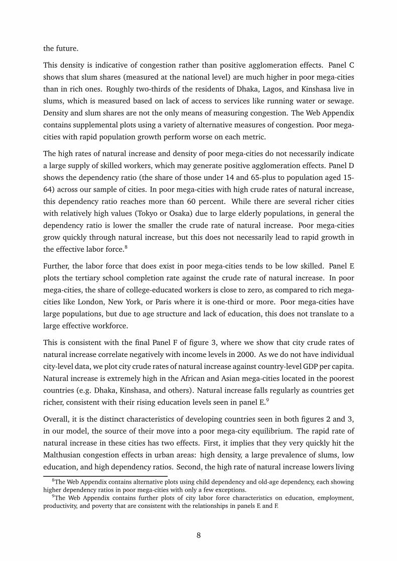
The dynamics can be most easily seen in a diagram. Figure 4 plots city population, Nu, against
wages, w. In the figure, the curves defined by N(w, mu) and N(w, mu) are plotted, and note
that at every wage N(w, mu)< N(w, mu), as noted in Lemma 2. Three initial points are plotted
with equal wages, but with varying initial city sizes.
Below N(w, mu), the city starts small enough that wage growth is positive and sufficient to
lower population growth fast enough to sustain wage growth indefinitely. This city becomes a
rich mega-city. Between N(w, mu) and N(w, mu), in the shaded area, wage growth is positive
at first but is not sufficient to lower the absolute population growth far enough to overcome
the effects of congestion. Eventually this city transitions into the third zone on the figure,
where Nu > N(w, mu), and wage growth becomes negative. This city becomes a poor mega-
city eventually.
Finally, the city starting with Nu > N (w, mu) is already so large that congestion effects are
sufficient to overwhelm productivity growth and the wage shrinks as the city grows. This city
is a poor mega-city as well.
The figure shows that the initial position of the city relative to the N(w, mu) curve is crucial
for determining the long-run outcome. Only cities that have a combination of high wages
and/or low population are able to experience fast enough wage growth to overcome the drag
of congestion effects.
The model indicates the poor mega-cities have wages that collapse to zero in the long-run. We
can easily allow for non-zero long-run wages in poor mega-cities by allowing for a minimum
level of earnings in the urban technology. We show in the appendix how to incorporate an
informal urban sector into the analysis that provides just such a minimum level of earnings.
Productivity growth in this informal technology would allow for wage growth in poor mega-
cities over time, but this wage growth would fall below rich mega-cities under most reasonable
19
assumptions.
4.4 The Rise of Poor Mega-Cities
Given our model, how do we explain the divergence of poor mega-cities from the historical
norms? As noted in the introduction, we focus on the distinct change in demographics
following the mortality transition that occurred after World War II. Recall from Figure 2 that
crude death rates in developing cities fell dramatically relative to their crude birth rates, and
thus the crude rate of natural increase in developing cities became very large. We propose that
in developing countries after the mortality transition, mu fell below a critical threshold that
pushed these cities into the poor mega-city equilibrium. Formally, in our model the following
proposition holds.
Proposition 2. For any given initial conditions w(0) and Nu(0) there is a threshold level mu such
that
• if mu ≤ mu the city becomes a Poor Mega-City
• if mu > mu the city becomes a Rich Mega-City
Proof. Please see appendix.
Low mortality cities become poor mega-cities because their population growth proceeds too
quickly. But note that the proposition implies that there is a non-linear effect of mu on city
development. Cities with mortality rates just above and just below the threshold mu can look
very similar at first, but the slightly faster natural increase in a city with a low mortality rate
will eventually create congestion effects that cannot be overcome. Differences in mortality
rates need not be large to generate significant long-run differences between poor and rich
mega-cities.
The difference between these poor mega-cities and their historical peers can be seen most
easily in Figure 5. Think of the pre-mortality transition demographics as being measured by
mPreu> mu, implying a low growth rate of urban population due to the high mortality rates in
urban areas. In comparison, developing countries after the mortality transition faced a much
higher level of population growth, because mPostu< mu.
In Figure 5 we have plotted both N(w, mPreu), the pre-mortality transition curve, and
N(w, mPostu), the post-mortality transition curve. We have also noted initial conditions of w(0)
and Nu(0). Given these initial conditions, after the mortality transition Nu(0)> N(w(0), mPostu)
and wage growth was negative as city size grew so fast it overwhelmed productivity growth.
This kept wages low, and because wages were low population growth continued at a rapid rate,
which in turn kept wages low. Poor mega-cities became stuck in the bad equilibrium.
20
Compare this to a historical city with identical initial conditions, but prior to the mortality
transition. In this case Nu(0) < N (w(0), mPreu), and city growth was slow enough that wages
were able to grow. This city was able to become a rich mega-city. Its wage growth was
sufficiently high to reduce population growth, and that in turn ensured that wage growth
remained high. They found themselves in the good equilibrium. The mortality transition
came to the historically rich mega-cities as well, later in their development. By beginning to
grow prior to the mortality transition, though, they would have been able to reach a high
enough wage that once the mortality transition did hit, they still had Nu < N (w, mPostu), and
thus were able to continue having growth in wages.
Note in the Figure that cities developed into poor mega-cities even though they may have
shared the same initial conditions and productivity growth as historical cities. Developing
country cities did not necessarily have to start out poorer or larger than their historical
counterparts in order to become poor mega-cities. The mortality transition was sufficient
to push them into that outcome. Of course, technology levels (Au(0)), productivity growth
(g), the strength of congestion effects (λ), and the exact relationship of population growth
to income (n(w, mu)) could all be different between historical cities and those in developing
countries. Those factors would alter the position or shape of the N (w, mu) curve, generating
differences in the long-run outcomes for cities. Those other factors are not irrelevant to the
growth of poor mega-cities, but the shift in mortality rates seen after World War II deserves
particular attention given the departure from historical norms.
5. DISCUSSION AND CONCLUSION
The model we developed relates city population growth to agglomeration and congestion in
those cities. It shows that wages in a city are not simply a function of productivity levels or
growth rates, but depend also on demographic behaviors. It is a general framework that can
be used to understand the dynamics of both city size and wage levels over time.
The model shows that small differences in population growth rates in emerging mega-cities
can result in very different long-run outcomes. We used this to explain the rise of poor mega-
cities after World War II, attributing it in part to the severe decline in death rates that occurred
because of the mortality transition. These lower death rates led these mega-cities to grow so
fast in absolute terms that the congestion effects overwhelmed productivity growth and led to
lower wages, which in turn perpetuated high population growth rates. This spiral led to the
poor mega-cities of today.
A critical implication of the model is that the poor mega-city equilibrium is stable. Once upon
that path a city will remain a poor mega-city indefinitely, even if it shares the same underlying
rate of productivity growth as rich mega-cities. The poor mega-cities of today are not simply
in a transitional state towards becoming the next New York or Tokyo, but rather have grown
21
so fast they are actively working against their own prosperity.
As in standard Malthusian models, our model implies that it takes a significant shift in
demographic behavior to break out of a poor equilibrium. Examples of these shifts and the
possibility of breaking out of the poor mega-city equilibrium exist. China’s one-child policy was
a severe brake on population growth, bringing crude rates of natural increase in major cities
close to zero. Now mega-cities like Beijing, Chongqing, Guangzhou, and Shanghai look similar
to historical mega-cities, growing only through in-migration from rural areas and generating
sustained growth in living standards.
At the other end of the scale we have the currently rich mega-cities that grew slowly over
time, which allowed productivity growth to stay ahead of congestion. One question is how
these cities have become so large (e.g. Tokyo with 38 million residents) while avoiding the
issues of poor mega-cities. As our model indicates, it is the relative growth rate of productivity
and absolute growth of population that determine wage growth. The level of population does
not necessarily dictate outcomes. There is nothing in our model dictating that rich mega-cities
must stay below a certain absolute cap in size. Aside from the theoretical considerations, these
rich mega-cities obviously invested in alleviating congestion as they grew. While we did not
discuss this explicitly, one could easily imagine that the effect of congestion (our parameter λ)
as an endogenous decision. At some threshold of total city revenues, for example, it is possible
to invest in congestion-alleviating technologies like sewage systems and subways. Rich mega-
cities were able to hit that threshold because their wages and population size grew, while poor
mega-cities are unable to hit the threshold because wages remain low even while population
grows.
Other explanations for the nature of poor mega-cities certainly exist. Urban bias, changing
preferences, and rural over-crowding are just some of the possibilities. While we focused on
mortality changes, our model is flexible enough to incorporate those alternatives easily. It
provides a way of understanding how these other factors may change cities dynamically, and
highlights that the effect of these factors on demographics are likely just as important as their
effects on city productivity or congestion.
The rise of poor mega-cities is a distinct shift from the historical experience. Given the sheer
numbers of people involved, understanding these cities is an important part of understanding
growth and development in general. Urbanization is often presumed to be synonymous with
economic growth, but the evidence on these poor mega-cities and the implications of our model
suggest that this is too broad a generalization. It is entirely possible for poor mega-cities to
appear and persist in poverty given their rapid growth in population. We cannot presume that
these poor mega-cities represent the initial stages of rapid economic development. Rather,
they may indicate traps that cannot be escaped from.
22
REFERENCES
Acemoglu, Daron, and Simon Johnson. 2007. “Disease and Development: The Effect of Life Expectancy onEconomic Growth.” Journal of Political Economy, 115(6): 925–985.
Ades, Alberto F, and Edward L Glaeser. 1995. “Trade and Circuses: Explaining Urban Giants.” The Quarterly
Journal of Economics, 110(1): 195–227.Allen, Robert C. 2001. “The great divergence in European wages and prices from the Middle Ages to the First
World War.” Explorations in Economic History, 38(4): 411–447.Allen, Robert C., Jean-Pascal Bassino, Debin Ma, Christine Mollâ-Murata, and Jan Luiten Van Zanden.
2011. “Wages, prices, and living standards in China, 1738-1925: in comparison with Europe, Japan, andIndia.” Economic History Review, Economic History Society, 64(s1): 8–38.
Ashraf, Quamrul, and Oded Galor. 2011. “Dynamics and stagnation in the malthusian epoch.” American
Economic Review, 101(5): 2003–41.Ashraf, Quamrul H., David N. Weil, and Joshua Wilde. 2011. “The Effect of Interventions to Reduce Fertility
on Economic Growth.” National Bureau of Economic Research Working Paper 17377.Barrios, Salvador, Luisito Bertinelli, and Eric Strobl. 2006. “Climatic Change and Rural-Urban Migration: The
Case of Sub-Saharan Africa.” Journal of Urban Economics, 60(3): 357–371.Becker, Gary S. 1960. “An Economic Analysis of Fertility.” In Demographic and Economic Change in Developed
Countries. NBER Chapters, 209–240. National Bureau of Economic Research, Inc.Becker, Gary S., Edward L. Glaeser, and Kevin M. Murphy. 1999. “Population and Economic Growth.” American
Economic Review, 89(2): 145–149.Bleakley, Hoyt. 2007. “Disease and Development: Evidence from Hookworm Eradication in the American South.”
The Quarterly Journal of Economics, 122(1): 73–117.Bleakley, Hoyt. 2010. “Malaria Eradication in the Americas: A Retrospective Analysis of Childhood Exposure.”
American Economic Journal: Applied Economics, 2(2): 1–45.Bleakley, Hoyt, and Fabian Lange. 2009. “Chronic Disease Burden and the Interaction of Education, Fertility,
and Growth.” The Review of Economics and Statistics, 91(1): 52–65.Chandler, Tertius. 1987. Four Thousand Years of Urban Growth: An Historical Census. Lampeter, UK: The Edwin
Mellen Press.Christakos, George, Ricardo A. Olea, Mark L. Serre, Hwa-Lung Yu, and Lin-Lin Wang. 2005. Interdisciplinary
Public Health Reasoning and Epidemic Modeling: The Case of Black Death. New York:Springer.Cutler, David, Winnie Fung, Michael Kremer, Monica Singhal, and Tom Vogl. 2010. “Early-Life Malaria
Exposure and Adult Outcomes: Evidence from Malaria Eradication in India.” American Economic Journal:
Applied Economics, 2(2): 72–94.Davis, James C., and J. Vernon Henderson. 2003. “Evidence on the Political Economy of the Urbanization
Process.” Journal of Urban Economics, 53(1): 98–125.Davis, Kingsley. 1956. “The Amazing Decline of Mortality in Underdeveloped Areas.” American Economic Review
Papers and Proceedings, 46: 305–18.Duranton, Gilles. 2008. “Viewpoint: From Cities to Productivity and Growth in Developing Countries.” Canadian
Journal of Economics, 41(3): 689–736.Duranton, Gilles. 2013. “Growing through Cities in Developing Countries.” Unpublished manuscript, Wharton
School, University of Pennsylvania.Duranton, Gilles, and Diego Puga. 2004. “Micro-foundations of urban agglomeration economies.” In Handbook
of Regional and Urban Economics. Vol. 4 of Handbook of Regional and Urban Economics, , ed. J. V. Hendersonand J. F. Thisse, Chapter 48, 2063–2117. Elsevier.
Fay, Marianne, and Charlotte Opal. 2000. “Urbanization without growth : a not-so-uncommon phenomenon.”The World Bank Policy Research Working Paper Series 2412.
Galor, Oded. 2011. Unified Growth Theory. Princeton, NJ:Princeton University Press.Galor, Oded, and David Weil. 1999. “From Malthusian Stagnation to Modern Growth.” American Economic
Review, 89(2): 150–154.Galor, Oded, and David Weil. 2000. “Population, Technology, and Growth: From Malthusian Stagnation to the
Demographic Transition and Beyond.” American Economic Review, 90(4): 806–828.Glaeser, Edward L. 2013. “A World of Cities: The Causes and Consequences of Urbanization in Poorer Countries.”
National Bureau of Economic Research, Inc NBER Working Papers 19745.Gollin, Douglas, Remi Jedwab, and Dietrich Vollrath. 2015. “Urbanization with and without Industrialization.”
working paper.
23
Henderson, J. Vernon. 1974. “The Size and Types of Cities.” American Economic Review, 64(4): 640–656.Henderson, J. Vernon. 2003. “The Urbanization Process and Economic Growth: The So-What Question.” Journal
of Economic Growth, 8(1): 47–71.Henderson, J. Vernon. 2010. “Cities and Development.” Journal of Regional Science, 50(1): 515–540.
Henderson, Vernon, Adam Storeygard, and Uwe Deichmann. 2013. “Has Climate Change PromotedUrbanization in Sub-Saharan Africa?” Unpublished manuscript, Department of Economics, Brown University.
Jedwab, Remi. 2013. “Urbanization without Industrialization: Evidence from Consumption Cities in Africa.”Unpublished manuscript, Department of Economics, George Washington University.
Jedwab, Remi, Luc Christiaensen, and Marina Gindelsky. 2014. “Rural Push, Urban Pull and ... Urban Push?New Historical Evidence from Developing Countries.” Working Paper.
Jones, Larry E., Alice Schoonbroodt, and Michele Tertilt. 2010. “Fertility Theories: Can They Explain theNegative Fertility-Income Relationship?” In Demography and the Economy. NBER Chapters, 43–100. NationalBureau of Economic Research, Inc.
Kremer, Michael. 1993. “Population Growth and Technological Change: One Million B.C. to 1990.” The Quarterly
Journal of Economics, 108(3): pp. 681–716.Lagerlof, Nils-Petter. 2003. “Mortality and Early Growth in England, France and Sweden.” Scandinavian Journal
of Economics, 105(3): 419–440.Maddison, Angus. 2008. Statistics on World Population, GDP and Per Capita GDP, 1-2008 AD. Groningen: GGDC.
Özmucur, Süleyman, and Sevket Pamuk. 2002. “Real Wages and Standards of Living in the Ottoman Empire,1489-1914.” Journal of Economic History, 62(2): 293–321.
Preston, Samuel H. 1975. “The Changing Relation between Mortality and Level of Economic Development.”Population Studies, 29: 231–48.
Stolnitz, George J. 1955. “A Century of International Mortality Trends: I.” Population Studies, 9: 24–55.Strulik, Holger, and Jacob L. Weisdorf. 2008. “Population, food, and knowledge: A simple unified growth
theory.” Journal of Economic Growth, 13(3): 195–216.United Nations. 2014. World Urbanization Prospects: The 2014 Revision. New York: United Nations, Department
of Economic and Social Affairs.Voigtländer, Nico, and Hans-Joachim Voth. 2009. “Malthusian Dynamism and the Rise of Europe: Make War,
Not Love.” American Economic Review Papers and Proceedings, 99(2): 248–54.Voigtländer, Nico, and Hans-Joachim Voth. 2013a. “How the West ‘Invented’ Fertility Restriction.” American
Economic Review, 103(6): 2227–64.
Voigtländer, Nico, and Hans-Joachim Voth. 2013b. “The Three Horsemen of Riches: Plague, War, andUrbanization in Early Modern Europe.” Review of Economic Studies, 80(2): 774–811.
World Bank. 2009. World Development Report 2009: Reshaping Economic Geography. Washington DC: World BankPublications.
World Bank. 2013. World Development Indicators. Washington D.C.: World Bank.Young, Alwyn. 2005. “The Gift of the Dying: The Tragedy of Aids and the Welfare of Future African Generations.”
The Quarterly Journal of Economics, 120(2): 423–466.
24
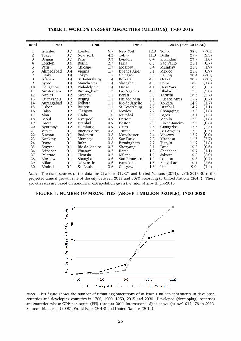
TABLE 1: WORLD’S LARGEST MEGACITIES (MILLIONS), 1700-2015
Rank 1700 1900 1950 2015 (% 2015-30)
1 Istanbul 0.7 London 6.5 New York 12.3 Tokyo 38.0 (-0.1)2 Tokyo 0.7 New York 4.2 Tokyo 11.3 Delhi 25.7 (2.3)3 Beijing 0.7 Paris 3.3 London 8.4 Shanghai 23.7 (1.8)4 London 0.6 Berlin 2.7 Paris 6.3 Sao Paulo 21.1 (0.7)5 Paris 0.5 Chicago 1.7 Moscow 5.4 Mumbay 21.0 (1.9)6 Ahmedabad 0.4 Vienna 1.7 Buenos Aires 5.1 Mexico 21.0 (0.9)7 Osaka 0.4 Tokyo 1.5 Chicago 5.0 Beijing 20.4 (-0.1)8 Isfahan 0.4 St. Petersburg 1.4 Kolkata 4.5 Osaka 20.2 (-0.1)9 Kyoto 0.4 Manchester 1.4 Shanghai 4.3 Cairo 18.8 (1.8)10 Hangzhou 0.3 Philadelphia 1.4 Osaka 4.1 New York 18.6 (0.5)11 Amsterdam 0.2 Birmingham 1.2 Los Angeles 4.0 Dhaka 17.6 (3.0)12 Naples 0.2 Moscow 1.1 Berlin 3.3 Karachi 16.6 (2.7)13 Guangzhou 0.2 Beijing 1.1 Philadelphia 3.1 Buenos Aires 15.2 (0.7)14 Aurangabad 0.2 Kolkata 1.1 Rio de Janeiro 3.0 Kolkata 14.9 (1.7)15 Lisbon 0.2 Boston 1.1 St. Petersburg 2.9 Istanbul 14.2 (1.1)16 Cairo 0.2 Glasgow 1.0 Mexico 2.9 Chongqing 13.3 (1.8)17 Xian 0.2 Osaka 1.0 Mumbai 2.9 Lagos 13.1 (4.2)18 Seoul 0.2 Liverpool 0.9 Detroit 2.8 Manila 12.9 (1.8)19 Dacca 0.2 Istanbul 0.9 Boston 2.6 Rio de Janeiro 12.9 (0.6)20 Ayutthaya 0.2 Hamburg 0.9 Cairo 2.5 Guangzhou 12.5 (2.3)21 Venice 0.1 Buenos Aires 0.8 Tianjin 2.5 Los Angeles 12.3 (0.5)22 Suzhou 0.1 Budapest 0.8 Manchester 2.4 Moscow 12.2 (0.0)23 Nanking 0.1 Mumbay 0.8 Sao Paulo 2.3 Kinshasa 11.6 (3.7)24 Rome 0.1 Ruhr 0.8 Birmingham 2.2 Tianjin 11.2 (1.8)25 Smyrna 0.1 Rio de Janeiro 0.7 Shenyang 2.1 Paris 10.8 (0.6)26 Srinagar 0.1 Warsaw 0.7 Roma 1.9 Shenzhen 10.7 (1.1)27 Palermo 0.1 Tientsin 0.7 Milano 1.9 Jakarta 10.3 (2.0)28 Moscow 0.1 Shanghai 0.6 San Francisco 1.9 London 10.3 (0.7)29 Milan 0.1 Newcastle 0.6 Barcelona 1.8 Bangalore 10.1 (2.6)30 Madrid 0.1 St. Louis 0.6 Glasgow 1.8 Lima 9.9 (1.4)
Notes: The main sources of the data are Chandler (1987) and United Nations (2014). % 2015-30 is theprojected annual growth rate of the city between 2015 and 2030 according to United Nations (2014). Thesegrowth rates are based on non-linear extrapolation given the rates of growth pre-2015.
FIGURE 1: NUMBER OF MEGACITIES (ABOVE 1 MILLION PEOPLE), 1700-2030
Notes: This figure shows the number of urban agglomerations of at least 1 million inhabitants in developedcountries and developing countries in 1700, 1900, 1950, 2015 and 2030. Developed (developing) countriesare countries whose GDP per capita (PPP, constant 2011 international $) is above (below) $12,476 in 2013.Sources: Maddison (2008), World Bank (2013) and United Nations (2014).
25
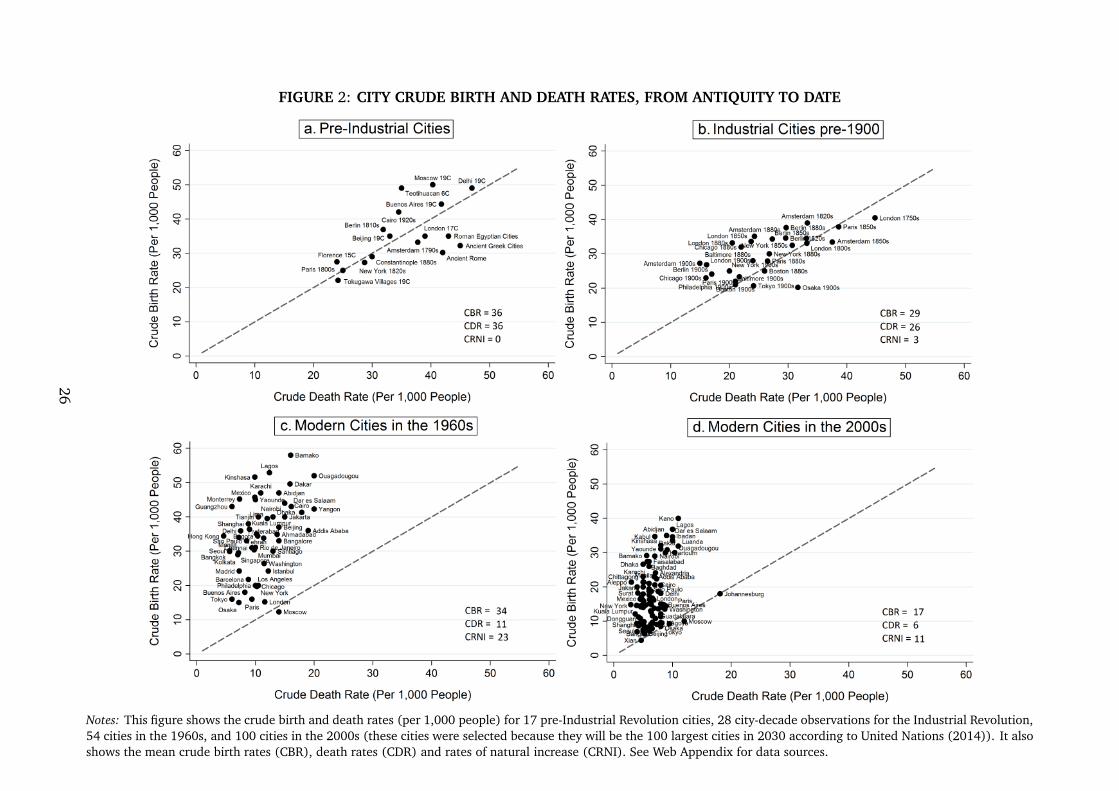
FIGURE 2: CITY CRUDE BIRTH AND DEATH RATES, FROM ANTIQUITY TO DATE
Notes: This figure shows the crude birth and death rates (per 1,000 people) for 17 pre-Industrial Revolution cities, 28 city-decade observations for the Industrial Revolution,54 cities in the 1960s, and 100 cities in the 2000s (these cities were selected because they will be the 100 largest cities in 2030 according to United Nations (2014)). It alsoshows the mean crude birth rates (CBR), death rates (CDR) and rates of natural increase (CRNI). See Web Appendix for data sources.
26
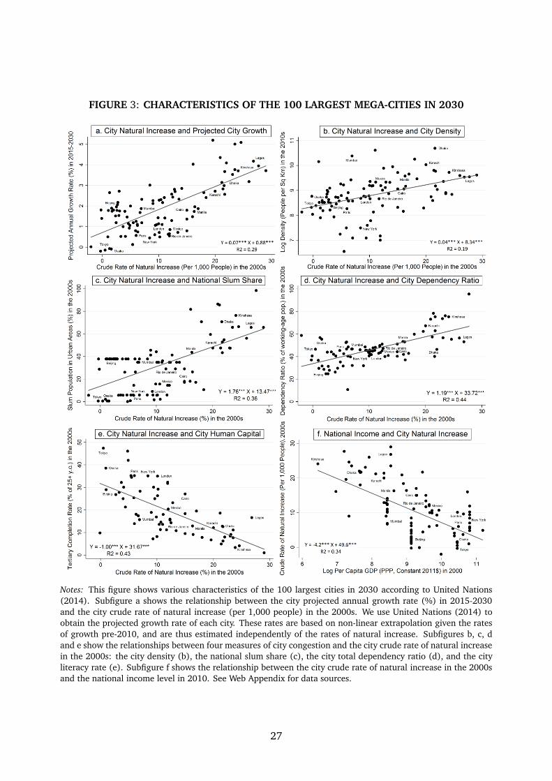
FIGURE 3: CHARACTERISTICS OF THE 100 LARGEST MEGA-CITIES IN 2030
Notes: This figure shows various characteristics of the 100 largest cities in 2030 according to United Nations(2014). Subfigure a shows the relationship between the city projected annual growth rate (%) in 2015-2030and the city crude rate of natural increase (per 1,000 people) in the 2000s. We use United Nations (2014) toobtain the projected growth rate of each city. These rates are based on non-linear extrapolation given the ratesof growth pre-2010, and are thus estimated independently of the rates of natural increase. Subfigures b, c, dand e show the relationships between four measures of city congestion and the city crude rate of natural increasein the 2000s: the city density (b), the national slum share (c), the city total dependency ratio (d), and the cityliteracy rate (e). Subfigure f shows the relationship between the city crude rate of natural increase in the 2000sand the national income level in 2010. See Web Appendix for data sources.
27
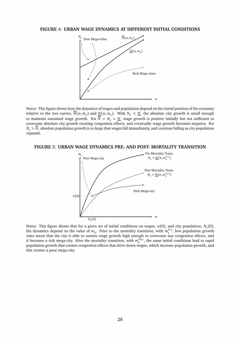
FIGURE 4: URBAN WAGE DYNAMICS AT DIFFERENT INITIAL CONDITIONS
Nu
w
N (w, mu)
N (w, mu)
b
b
b
Rich Mega-cities
Poor Mega-cities
Notes: This figure shows how the dynamics of wages and population depend on the initial position of the economyrelative to the two curves, N(w, mu) and N(w, mu). With Nu < N , the absolute city growth is small enoughto maintain sustained wage growth. For N > Nu > N , wage growth is positive initially but not sufficient toovercome absolute city growth creating congestion effects, and eventually wage growth becomes negative. ForNu > N , absolute population growth is so large that wages fall immediately, and continue falling as city populationexpands.
FIGURE 5: URBAN WAGE DYNAMICS PRE- AND POST- MORTALITY TRANSITION
Nu
w
Post Mortality Trans.Nu = N (w, mPost
u)
Pre Mortality Trans.Nu = N(w, mPre
u)
b
Rich Mega-city
Poor Mega-city
Nu(0)
w(0)
Notes: This figure shows that for a given set of initial conditions on wages, w(0), and city population, Nu(0),the dynamics depend on the value of mu. Prior to the mortality transition, with mPre
u, low population growth
rates mean that the city is able to sustain wage growth high enough to overcome any congestion effects, andit becomes a rich mega-city. After the mortality transition, with mPost
u, the same initial conditions lead to rapid
population growth that creates congestion effects that drive down wages, which increase population growth, andthis creates a poor mega-city.
28