JOURNAL OF DIFFERENTIAL EQUATIONS 69, 31fk-321 (1987)

The Monotonicity of the Period Function for Planar Hamiltonian Vet--r Fields

CARMEN CHICONE *

Depnrtment of Mathemnttcs, Umaersity of Missourt, Columbia, Missouri 6821 I

Received December 23, 1985; revised January 27, 1987

If the Hamiltoman system with Hamiltoman H(X, v) = +yz + I’(X) has a center at

the origin it is shown that the period function for the family of periodic trajectories surrounding the center is tnonotone when the function c//iv’~’ is convex. This theorem is applied to determine existence and uniqueness of solutions for the Neumann boundary value problem X” = a(.~‘)~ + bs + c, s’(O) = s’( 1) = 0. C’ 1937 Academic Press, Inc.

I. INTRODUCTION

We consider classical Hamiltonian systems on the plane with Hamiltonians of the form H(x, ~1) = +I>‘+ C’(x), where V is a smooth potential function with a nondegenerate relative minimum at the origin. The phase portrait of the Hamiltonian vector field X= ~~(a/&- V’(X)(~/C~J~) has a center at the origin surrounded by periodic orbits each of which is a level energy curve of H with energy EE (0, E,). In this article we study the period function T: (0, E, j + R which assigns to each periodic orbit its minimum period. In order to state our main result we let K(E) = {x E K: V(x) ,( Ej and define

N(x) = 6V(x)( V”(s))‘- 3( V’(x))’ V”(x) - 2V(x) V’(x) V”‘(x)

V(x) ” = (WY))” (m

>

We have the following theorem.

THEOREM A. If N(x) 2 0 for all x E K(E), then T is monotone increasing

on (0, E). If N(x) < 0 for ull x E K(E). then T is monotone decreasing on

(0, El.

* Research funded in part by a grant from the Research Council of the Graduate School, University of Missouri-Columbia.

310 0022-0396/X7 $3.00

MIONOTONICITYOF PERIOD FUN<'TIONS 311

The period function has been extensively studied by a number of dif- ferent authors, especially [3, 5, 6, 1 l-171. It is perhaps remarkable that so many different methods of analysis have been applied to this problem. Our observation that the monotonicity of the period function is implied by the convexity of the function V(x)/r”(x))’ seems to bc new. However, our results are similar in spirit to the work of Chow and Wang [6 3 which came to our attention during the preparation of this paper. It seems that both papers were motivated by a desire to understand the potential V(X) = eY - s - 1 which resists analysis by previous methods. Monotonicity of the associated period function follows from our results and those of Chow and Wang.

2. THE PROOF OF THEOREM A

Since each trajectory of X is a level curve of I-i the phase portrait is sym- metric with respect to the .y-axis. Thus. the period of the periodic orbit with energy E is given by

T=2 “I& 2 j“ 1

d.u

‘it, !: ,i5 w &5- V(x)’

where sg and x, denote the left and right intersections of the curve given by i J.’ + V(x) = E with the -u-axis. We observe that T is a convergent improper Riemann integral.

In order to express the integral so that we can compute dT/dE we con- sider a change of variables. Dclinc

V(x) ’ = X

h(s) =

I ( > 7 .y- ) x E fq E)‘?. ( 0 )

0, x = 0.

Since V has a quadratic minimum at the origin h is smooth. Moreover, it is easy to see that h’(x) > 0 for all x E K( E,) so h is monotone increasing. Set r = II(X) and change variables in the integral to obtain

This form of the integral suggests the further substitution r = \,%sin 0. After this change of variables we obtain

d0

h’(h- l(jEsin 0))

312 CARMEN CHICONE

With the integral in this form we can differentiate to obtain

dT 1 r lii2

J -h”(h -=- ‘(fi sin 0)) sin 0 de

dE &E -n/2 (h’(h-‘(*sin e)))3

Next we integrate by parts. For this computation it is convenient to set .Y = h-‘(,/?? sin 0) and separate the integrand as

-a(sin 0 de).

Then,

d.v fi cos u

z=h’(h-‘(fisin 0))

and

dT h”(x) x:2

E= ,/%(hr(x))3 cos 0

II;2

rn;2

+& n;2

3(h”(x))’ - h’(x) h”‘(x) cos o d’r de

(h’(x)T’ d0

7~,7 =-$Lrj2

3(/~“(x))~ - h’(x) h”‘(x)

(h’(x)15 cos2 8 de.

Finally, using h2(x) = V(X), it is easy to compute

h’=;, h,, = 2 Vv’ - ( V)’

4h’

and

h,,,=4V2V”‘-6VV’V”+3(V’)3 8h V’

from which we obtain

3(h”)2 - h’h”’ = ~V’(IJ”‘)~-~(V’)~ V”-2VV’V” 8 V’

3. APPLICATIONS

We consider some examples to illustrate the application of Theorem A.

MONOTONICITY OF PERIOD FUNCTIONS 313

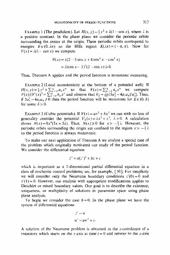
EXAMPLE 1 (The pendulum). Let H(x, JP) = t y2 + 1( 1 - cos x), where i, is a positive constant. In the phase plane we consider the periodic orbits surrounding the center at the origin. These periodic orbits correspond to energies E E (0, ,‘.rr) so the Hills region K(,?n) = ( -n, n). Now for V(X) = E.( 1 - cos x) we compute

N(x) = A(2 - 5 cos .K + 4 cos2 x - cos3 x)

= %(cos x - I)‘(2 - cos x) >, 0.

Thus, Theorem A applies and the period function IS monotone increasing.

EXAYPLE 2 (Local monotonicity at the bottom of a potential well) If H(s, y) = t y* + z;- z a,~” so that V(X) = C,“-? LI,X” we compute V(x)/( r(x)’ = x:,“=O h,,x” and observe that h, = &((5a: - 4azu,),faz). Thus, if 5~1: - 4a,a, #O then the period function will be monotone for EE (0,6) for some 6 > 0.

EXAMPLE 3 (Cubic potentials). If V(x) = us-’ + hx’ we can with no loss of generality consider the potential V,(x) = /Ix2 + x3, i. > 0. A calculation shows IV(X) = 6x4(3x + 5i). Thus, X(s) 2 0 for x > -s i.. However, the periodic orbits surrounding the origin arc confined to the region x > - f i. so the period function is always monotonic.

To make our next application of Theorem A we analyse a special case of the problem which originally motivated our study of the period function. We consider the differential equation

z” = a(z’)’ + bz + c

which is important as a I-dimensional partial differential equation in a class of stochastic control problems; see, for example, [lo]. For simplicity we will consider only the Neumann boundary conditions z’(O) =0 and z’( 1) = 0. However, our analysis with appropriate modifications applies to Dirichlet or mixed boundary values. Our goal is to describe the exislence, uniqueness. or multiplicity of solutions in parameter space using phase plane analysis.

To begin we consider the cast b=O. In the phase plane we have the system of differential equations

-” z ,y

w’ = aw2 + c.

A solution of the Neumann problem is obtained as the z-coordinate of a traiectory which starts on the z-axis at time t = 0 and returns to the z-axis

314 CARMEN CHICONE

at time t = 1. There are just two possibilities. If c # 0 all trajectories starting on the z-axis cross the z-axis in the same direction and thus never return so that the Neumann problem has no solutions. If c =0 all trajectories starting on the z-axis remain at their initial positions for all time and thus z(t) = const. gives infinitely many solutions.

When b # 0 the change of variables z = x - c/b transforms the Neumann boundary value problem to the equivalent problem

x” = a(.~‘)~ + bx

x’(0) = 0, x’( 1) = 0.

Again, we consider the differential equation in the phase plane where a solution is the x-coordinate of a trajectory of the system

x’=y

which starts on the x-axis and returns in one unit of time. We observe that the origin is the only stationary point for the phase flow and it corresponds to the trivial nonoscillatory solution x(t) = 0 of the Neumann problem.

If b > 0 the origin in the phase plane is a hyperbolic saddle point for the phase flow. Any orbit which starts at (x,, 0) for x0 > 0 enters the upper half plane and drifts to the right (since x’ > 0 in the upper half plane). But, since the vector field ~(a/ax) + (bx + uy2j(i3/dy) always points into the upper half plane along the positive x-axis the orbit can not return to the x-axis. Similarly, an orbit starting at (x0, 0) for x0 < 0 enters the lower half plane, drifts left and cannot return to the x-axis. Thus, for b > 0 the Neumann problem has no nontrivial solution.

The case b < 0 is the most interesting case because the origin is a center surrounded by periodic orbits of the phase flow and the possibility of oscillatory solutions exists. We will say a solution has n nodes in case the corresponding trajectory in the phase plane crosses the y-axis exactly n times. In case a = 0 the system is linear and all phase trajectories other than the center are periodic with period 2x( - b)-~‘j2. Clearly, solutions with n nodes exist if and only if b = - (n7c)“; n = 1, 2, 3,.... Also, we have time reversal (due to the symmetry of the phase flow with respect to the x-axis), i.e., s(t) is a solution if and only if x( I- t) is a solution. Thus, there are infinitely many pairs of solutions with n nodes when b = ( --nn j’. When a # 0 we observe the system of differential equations has the integral

Using this integral it follows easily that the set of periodic orbits

MONOTONICITY OF PERIOD FUNCTIONS 315

surrounding the center is bounded by the (unbounded) separatrix given by the integral when k= 0. Moreover, it is easy to see there is no ioss of generality in assuming a > 0 because the phase portrait of the system with a t0 is identical to the phase portrait with a > 0 up to the symmetry f(x, v) = (-x, v). With this assumption in force we compute the time 5 required for the trajectory starting on the separatrix at (- 1/2a, 0) to reach infinity along the separatrix as

Since the linearized equations have all solutions periodic with period 2n( -b) ~ ‘!’ the period function T for this family of periodic orbits has range (2x( -b)-‘,‘2, cc).

We intend to show T is monotone but first we note the consequences. Using the time reversal property we again have oscillatory solutions existing in pairs. Hence, a solution with II nodes unique up to time reversal exists if and only if b < - (117c)~. Also, for fixed b < 0 at most a finite num- ber of solutions exist.

Finally, we show T is monotone when b < 0 and a> 0. To see this we compute the change of variables defined by

u = In (

b + 2a( bx + uy’ )‘ i b ,

2’ = 2aJl

and obtain the transformed system of differential equations

u’ = L’

u’ = b(e” - 1).

This system is in Hamiltonian form with Hamiltonian

H(u, u) = 4 u2 - b(e” - u - 1).

Hence, Theorem A will apply to show T is monotone as soon as we show V(x) = - b(e” - IV - 1) satisfies N(X) > 0 for all .Y E ( - a, orj ). We have

N(x) = ex(e2” - 4xex f 4e” - 2-r - 5) = e’F(x).

But, we compute F(O)=O, F(O)=O, and

F’(x) = 4ex(ex - x - 1) >, 0.

Thus, N(x) > 0 and T is monotone.

316 CARMEN CHICONE

In view of the analysis just completed, Example 2 and the results of [ 171 we know the period function is monotonic on the family of periodic orbits surrounding the center of a quadratic system which can be expressed in one of the three forms

y’ = - bx + q2,

x’ =)’

)I’ = - bx + cx’,

and

x’ = x( a - by)

y’=y(-c+dx).

It thus seems natural to ask if the same is true for any quadratic system with a center. This delicate question serves nicely as a test of the current state of knowledge about the period function. We are content here to make a few remarks about our attempt to apply Theorem A to this question.

Since all quadratic systems with centers are known and since the corresponding integrals can be given explicitly, see [18], there is ample opportunity to compute. We consider the system

u’ = t’

VI= -bbu+Au*+Buv+Cd

for which there is a center at the origin if and only if either B= 0 or C + A/b = 0. In case B = 0 we have already shown the monotonicity of the period function when AC = 0. For AC # 0 the substitution

z=ci2 bCt, J-

where CI = A/bC transforms the differential equation to the Hamiltonian form

1” = a4~2 ~(1-x)(ozln2(1-x)+ln(l-x))5

MONOTONICITY OF PERIOD FUNCTIONS 317

which has Hamiitonian

fax, y)=$‘+& ( ( (l--~)~ aln2(1-x)

l--Cc 1-a +(l-U)ln(l-xx)-- #+2

1 1

1 =zy”+ -& V(x).

In the new coordinates the center resides at the origin and the stationary point (1 - exp( - c( ~ ‘), 0) is one end point of the Hills region. Thus in the Hills region 1 -x > 0, the logarithms are defined and H is analytic. We compute

2cr+l 1 “““;x2--a x3-j--$x4+ ..‘,

whence by Example 2 the period function is monotone increasing in a neighborhood of the origin. Since the period approaches intinity as the periodic orbits approach their boundary separatrix there is evidence that the period is monotone. A calculation shows

-I- f (1 - x)‘(2a3L5 + (3~~ + 5a*) L4 + ( - 10a3 + 6a2 + 4cz) L3

+(10LY3-15a~+4a+1)Lz+10a2-11M+1)L-3(1-cr)),

where L=ln(l-x). At x=1-exp(--a-‘) we compute

N=&X*(l-cr)[l-a+e-2~~(1+C1)],

which is negative for LY > 1. Thus N is not always of constant sign and Theorem A does not apply directly. However, Theorem A does apply in special cases. For example, when a = 1,

N(x) = (1 - x)’ (ln’( 1 - x))(4 + ln( 1 - x)).

Here the Hills region is contained in the set x < 1 - exp( - 1) and N is always positive. Also, when c1= - 1 we compute

318 CARMEN CHICONE

where as above L = ln( 1 -x). The Hills region in terms of L is the interval (-co, 1) and again N is positive over the Hills region.

Actually, the case D! = - 1 corresponds to the system

u’ = v

A v’= -bu-+Au2--v2.

b

This system is transformed by the substitution

A 5 = - 11

b

to

x’=y

y’= --x+x2+.

A second substitution given by

w=l-((x+y)

z=l-(x-y)

transforms to the Volterra-Lotka system

w’ = w( 1 - z)

z’ = z( W’ - 1).

Thus, the monotonicity in case CI = - 1 is a special case of the results of

t-171. The case C + A/b = 0 is more difficult. We will again consider only some

special cases in this family. In case both A and C vanish we have the form

v’ = - bu + 2Buv,

MONOTONICITY OF PERIOD FUNCTIONS 319

for which the substitution

x = -; (II - BU2)

transforms the differential equation to the form

x’ = y

y’= -bbx+By’

and the period function is monotonic as shown by the discussion following Example 3.

EXAMPLE 4. This example is motivated by a desire to understand the behavior of the period function when the region containing periodic orbits has boundary points in the finite plane but none of them are stationary. For this we consider the system

2.4’ = v

u’= -u(b- av')

with a, b > 0 which has a center at the origin surrounded by periodic orbits which are bounded by the lines given by u = + (ba -‘)‘!2. The substitution

x= tanh-‘((abk’)%)

y = - (ab)‘12u

transforms the differential equation to

x’ = I

~1’ = -b tanh x,

which is in Hamiltonian form with Hamiltonian

H(x, y) = 4 y2 + b ln(cosh x).

Thus, we consider V(x) = ln(cosh x) and compute

N(x) = (sech2 x)(6 ln(cosh x) - 2 ln(cosh x) tanh’ x - 3 tanh’ x),

Since sech’ s is always positive it is enough to show

M(x) = 6 ln(cosh X) - 2 ln(cosh X) tanh” x - 3 tanh’ x >, 0.

3X6913-3

320 CARMEN CHICONE

Note that A4 is even and cash x is increasing for x>O. Thus, with z = cash x it suffkes to show

L(z)=M(cosh-‘~)=-$(6z~lnz--2(z’- 1) fnz--j(r2- l))>O

for z 2 1. To see this consider K(z) = z’L(z) and observe K( 1) = 0, K’( 1) = 0, and R’(z) > 0 for z 2 1.

We end this section with a question. If the differential equation

24’ = P(r.4, II)

u’ = Q(u, u)

has a center at the origin surrounded by a region R consisting of periodic orbits, when is there a change of coordinates defined on R such that in the new coordinates the differential equation is in Hamiltonian form with Hamiltonian

REFERENCES

1. V. I. ARNOLD, “Geometric Methods in the Theory of Ordinary Differential Equations,” Springer-Verlag, New York, 1983.

2. R. I. BOGDANOV, Bifurcation of limit cycle of a family of plane vector fields, Selecta Math. Soviet 1 (1981), 373-387.

3. J. CARR, S. N. CHOW, AND J. K. HALE, Abelian integrals and bifurcation theory, J. Oif- ferential Equations, in press.

4. S. N. CHOW AND J. K. HALE, “Methods of bifurcation Theory,” Springer-Verlag, New York, 1982.

5. S. N. CHOW AND J. A. SANDERS, On the number of critical points of the period, to appear. 6. S. N. CHOW AND D. WANG, On the monotonicity of the period function of some second

order equations, to appear. 7. R. H. CUSHMAN AND J. A. SANDERS, A codimension two bifurcation with a third order

Picard-Fuchs equations, Differemial Equations 59 (1985), 243-256. 8. S. B. HSU, A remark on the period of the periodic solution in the Lotka-Volterra systems,

J. Math. Anal. Appl. 95 (1983), 428-436. 9. Yu. IL’YASHENKO, The multiplicity of limit cycles arising from perturbations of the form

M” = P,/Q, of a Hamiltonian equation in the real and complex domain, .4mer. Marh. Sot. Tram-l. 118 (1982), 191-202.

10. J. M. LASRY AND P. L. LIONS, Equations elliptiques non lineaires avec conditions aux limites intinies et controle stochastique avec contraintes d&tat, C. R. .4cad. Sci. Paris, Ser. 1299, 7 (1984), 213-216.

11. W. S. LLXJD, Periodic solution of x” + cx’ +g(x) = &f(r). Menr. .4mer. Math. sot. 31(1959), l-57.

MONOTONICITY OF PERIOD FUNCTIONS 321

12. C. OBI, Analytical theory of nonlinear oscillation, VII, The periods of the periodic solutions of the equation x” + g(x) = 0, J. Math. Anal. Appl. 55 (1976), 295-301.

13. Z. OPIAL, Sur les piriodes des solutions de l’equation diffirentielle x” +g(x) =O, Amt. Polon. Math. LO (1961), 49-72.

t4. J. SBAOLLER AND A. WASSERMAN, Global bifurcation of steady-state solutions, 1. D@j%rm- tial Equations 39 ( 198 1 ), 269-290.

15. D. WANG, On the existence of 2x-periodic solutions of differential equation x” +g(x) =p(t), Chinese Ann. Mark No. 1 A 5 (1984), 61-72.

16. J. WALDVOGEL, The period in the Lotka-Volterra predator-prey model, SZ.4,w J. Numer. .4nal. 20 (1983).

17. J. WALDVOGEL, The period in the Lotka-Volterra system is monotonic. preprint. 18. V. LUNKEVICH AND K. SIBIRSKII, Integrals of a general quadratic differential system in

cases of a center, DiJfirential Equations 18 (1982) 563-568.