Embed Size (px)
Citation preview
Print Date: 3/25/2010
The Moderating Impact of Promotion on Substitution: An Economic Approach
Elina Petrova and Alan L. Montgomery
Working Draft, Do Not Distribute
March 2010
Elina Petrova is an Assistant Professor of Marketing at Washington State University and Alan L. Montgomery (e-mail: [email protected]) is an Associate Professor at the Tepper School of Business, Carnegie Mellon University, 5000 Forbes Ave., Pittsburgh, PA 15213.
Copyright © 2010 by Elina Petrova and Alan L. Montgomery, All rights reserved
Abstract
We show that there is an economically consistent way to introduce interactions between price and promotion. The model affords a more informative and comprehensive outlook on the impact of promotion on the demand elasticities in the category and enables interesting insights into the associated changes in consumer price sensitivity and spending proclivity. The main effect of promotions is that they increase market share. However, there are many other more subtle effects that depend upon the strength of the product. For example, as the category expands we find that superior products can benefit from promotions over weaker ones. The vulnerability of a product to competitor prices can be lessened if it is superior, while lesser products will experience increased price competition. The often discussed asymmetric competition between products can either be magnified or reduced by promotions. If promotional effects are strong enough then substitution between a promoted product and superior alternative can be depressed enough that we can see sign reversals in the cross-price elasticity between this promoted product and its non-promoted superior-alternative. Negative cross-price elasticities are persistent problems when estimating demand models in marketing applications, and promotions may provide an explanation for why these unexpected signs can occur for apparent substitutes.
Keywords: Economic Theory, Promotions, Substitution

- 1 -
1. Introduction
Promotions are a powerful and ubiquitous tool to spur demand and are almost always
accompanied by price discounts. Empirical research shows that promotions reinforce price
discounts and generate more in sales than a price discount alone (Blattberg, Briesch and Fox 1995).
Marketing models like Wittink et al. (1988) SCAN*PRO model or Guadagni and Little’s (1983) logit
model frequently incorporate interactions between price and promotions to capture this effect.
However, these direct interactions are often not consistent with economic models, and as a
consequence we lose the rich knowledge about demand afforded by economic theory. Our
objective is to show how promotions can interact with price in an economically consistent manner.
Our results yield insights into understanding how promotion moderates competition. Obviously
promotions tend to increase own product sales, but they can also confound existing substitution
patterns and under certain conditions increase the attractiveness of non-promoted products and led
to increases in their purchases.
The idea that promotions may have interact with price changes is empirically well supported
by empirical marketing research. Mulhern and Padgett (1995) finds evidence that buying promoted
items also induces customers to spend more on non-promoted items in the store. In a similar vein,
Heilman et al. (2002) find that unexpected in-store coupons induce customers to make more
unplanned purchases in general, as well as more unplanned purchases of treats, and more purchases
in categories that are in close physical proximity to the promoted ones. Heilman et al. (2002) call it
“the psychological income effect”. Using household data, Dreze et al (2004) find that consumer
shopping trips to supermarkets that include purchases of promoted dry goods result in households
that spend more on non-promoted items in that category than is spent on the entire category when

- 2 -
no promoted items are purchased. Finally, promotional elasticities have been shown to be distinctly
different from the attendant price elasticities (Lattin and Bucklin, 1989; Blattberg and Neslin, 1990).
Thus, the empirical evidence seems to indicate that promotions are more effective than a
commensurate price adjustment may suggest. From a classical economic perspective the
interactions between prices and promotions are perplexing, since promotions serve an educational
role which is often assumed away by complete information. The traditional assumptions concerning
transitivity and fungability of money also indicate that price promotions should have the same
impact as a price discount. An alternative behavioral theory is that an interaction between price and
promotion occurs because of reference price effects. However, this behavioral explanation may not
be consistent with a classical economic framework. If we reject an economic approach then the
desirable theoretical foundation provided by demand theory is lost.
Our objective is to understand if a classical economic approach can be extended to
incorporate non-traditional roles for promotion in moderating price discounts and changing
consumer perceptions of their expenditures. To achieve this aim we show how promotions can be
introduced by modifying price and expenditures with functions that depend on promotions, or what
we refer to simply as modifying functions. We adapt a method developed by Lewbel (1985) for
incorporating demographic variables into demand model to show how promotional variables can
also be incorporated. The advantage of this approach is that it generalizes to any demand system
and preserves the consistency of the original demand system.
The novelty and substantive value of our approach can also be found in its inferential
capabilities about how promotions moderate substitution. The main effect of promotions is that
they increase market share. However, there are many other more subtle effects that depend upon
the strength of the product. For example, as the category expands we find that superior products
- 3 -
can benefit from promotions of weaker ones. The vulnerability of a product to competitor prices
can be lessened if it is superior, while lesser products will experience increased price competition.
The often discussed asymmetric competition between products can either be magnified or reduced
by promotions. If promotional effects are strong enough then substitution between a promoted
product and superior alternative can be depressed enough that we can see sign reversals in the cross-
price elasticity between this promoted product and its non-promoted superior-alternative. Negative
cross-price elasticities are persistent problems when estimating demand models in marketing
applications, and promotions may provide an explanation for why these unexpected signs can occur
for apparent substitutes.
2. Introducing Price-Promotion Interactions through Modifying Functions
An economic approach to understanding sales response (Deaton and Muellbauer 1980) is
characterized by a consumer maximizing their direct utility function, *( )U q , which is a function of
the vector of n quantities 1 2* nq qq q consumed at their corresponding prices
1 2* np p p p , and subject to a constraint on expenditures *x :
*
* * * *max ( ) . . 'U s t xq
q p q (1)
The solution to this problem yields a system of Marshallian demand equations: * * *,i iq D x p .
Alternatively we could also consider the dual problem in which a consumer minimizes their
expenditures subject to a utility constraint:
*
* * * *min ' . . ( )x
x s t U u p q q (2)
- 4 -
The solution to this problem yields a system of Hicksian demand equations: * * *,i iq H u p .
Substitution of Hicksian demands into the expenditure equation yields the cost function:
* * *,x C u p . For the time being we suppress indices for consumer or store and time for all our
variables.
A common approach to incorporate exogenous variables, like demographics and
promotions, is to assume that the parameters of the utility function are themselves functions of
these variables. The problem is that this ad hoc introduction can destroy the consistency of the
economic approach. For example, the adding up, homogeneity, or Slutsky symmetry can be
destroyed or the concavity of the cost function may not hold. Suppose we employ a log-log demand
model (Montgomery and Rossi 1999) and presume that the price elasticity parameters are a function
of promotions then the homogeneity constraint is violated. In general the ad hoc introduction of
exogenous variables as functions of the parameters is problematic.
An alternative approach is to introduce promotions and other exogenous variables by
directly modifying price and expenditures. We posit that promotions operate by transforming
consumer’s perceptions of prices and expenditures. Lewbel (1985) provides a general treatment for
understanding what types of transformations are permissible and how an existing demand system or
cost function can be transformed into a new, consistent demand system. Although Lewbel’s
objective was to introduce demographic variables into a demand system the same methodology can
be used to introduce promotions and other marketing variables into a demand system.
The methodology derives a correspondence between the original (and potentially
unobserved) decision space and a new decision that incorporates observed variables of interest. For
example, in our analysis we could begin with an Almost Ideal Demand System (AIDS) model and
- 5 -
modify price and expenditures with promotion effects to derive a new AIDS model with promotion
effects. Instead of assuming that quantity, prices, and expenditures are directly observed in the
original demand system, we can instead think of these as intermediate goods. Our new variables can
be thought of as the observable quantities, and our modifying functions define the transformation of
these intermediate goods into the observable quantities.
In our research we focus our attention on the following class of modifying functions:
( ), exp( )i i i i i ip h p s p s , (3)
1
(1 )
1
/ , i i i i
ns s
ii
P Px x p
. (4)
Notice the variables with asterisk superscripts are assumed to be the shadow or effective variables
that are not directly observed. Specifically, x denotes the effective expenditure while x is the
observed expenditure, ip denotes the effective price while ip indicates the observed price, the
variable is is an indicators for the presence of promotions, and 1 2 ns s s s denotes the vector
of promotion variables. We consider the behavioral interpretation of these modifying functions in
subsection 2.1. It is trivial to remove promotions from the model by nullifying the parameters
( 0i and 0i ). Under this condition our intermediate variables are the same as the observable
ones: x x and i ip p .
Notice that equation (4) implicitly defines our new cost function:
* 1*, , , ( , ) , , , ( , ) i isx C u f C u h C u h P p s p s p s p s , (5)
where the vector is defined componentwise: * ( , )hp p s .

- 6 -
Additionally we must impose the following constraints on this transformation to ensure that
the cost function implied by our modifying function will be valid:
0 1i ii
s . (6)
Since our promotion variables must lie within the interval 0 to 1, this constraint implies that our
parameters must be non-negative and less than unity: 0 1i . This is also a sufficient condition if
only one product is promoted. A proof of the validity of our modifying functions is given in
Appendix A.
The importance of our modifying function is that we can express our new demand system in
terms of our original system. Following Lewbel (1985) we can show (see Appendix B3 for a
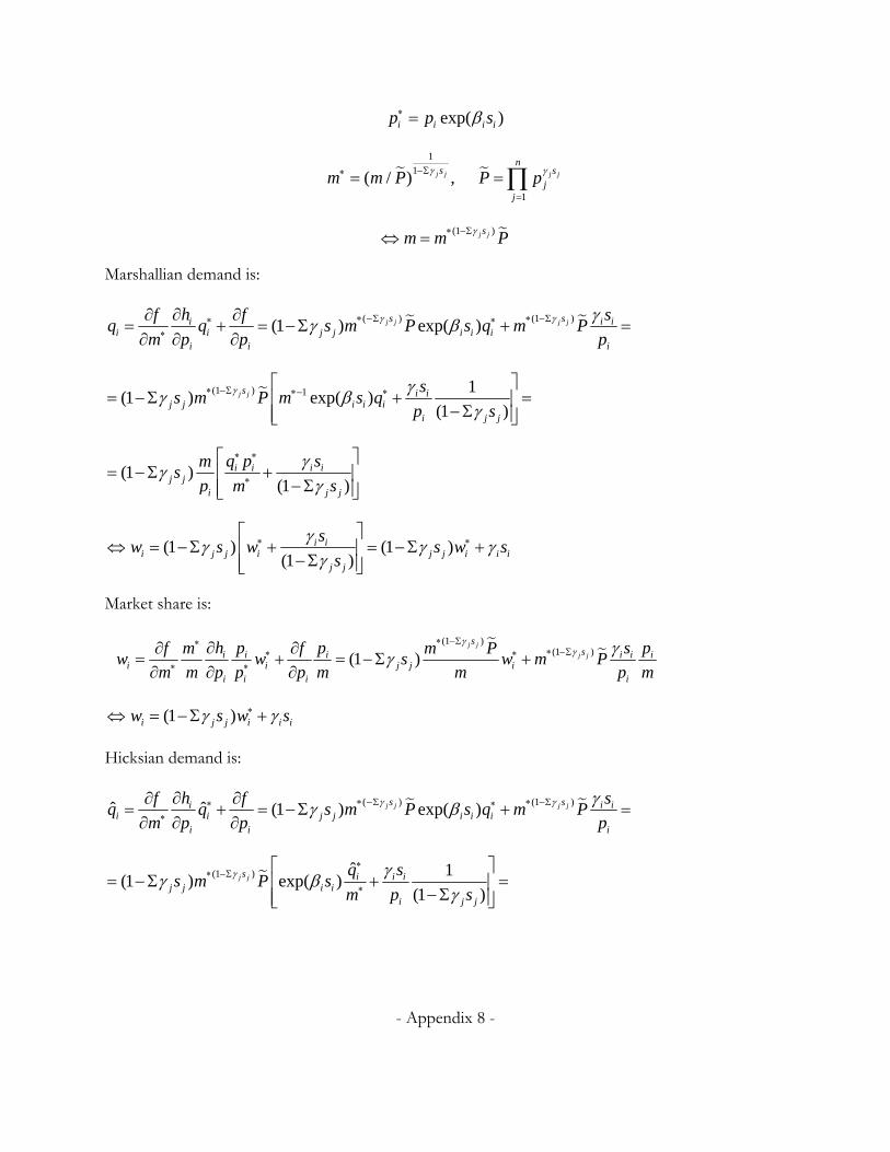
derivation) that that our modified Marshallian demand is:
(1
)
*
11 exp{ }
/ i i
i ii j j i i i
j is
sxq s s q x
pPx
. (7)
Hicksian demand is:
*
1(1 )
( , ,
(
)1 exp{
)}
/, , i i
i ii j j
si i i
j i
sC uq s s q x
pu PC
p s
p s. (8)
The budget shares or market shares ( iw and *iw ) are:
*1i j j i i ij
w s w s
, where i ii
p qw
x and
* **
*i i
i
p qw
x . (9)
Although it appears the share is a linear function of promotions, we point out that quantity and
expenditures have nonlinear dependencies on promotions.
- 7 -
Perhaps it is easiest to understand the relationship between the original and modified
demand systems using the budget share equation. In equation (9) we observe that promotions
translate demand and then rescale the original budget shares to guarantee adding up. Observe that
the translation in budget shares due to promotion guarantees that a promoted product will attain a
minimum share of i i iw s . Additionally, if a product is not promoted while other products are
promoted, then its budget share can never exceed the original budget share: *i iw w . Alternatively,
suppose that only a single competing product j is promoted (e.g., 0, 1,i js s i j ), then the share
of the remaining products are reduced proportionately: *(1 )i j j iw s w .
Our choice of a modifying function for price is driven by our desire to rescale price, for
example promotions may reinforce price declines and make them appear more substantial. We also
considered power transformations of price with functions of promotions in the power, but these
transformations violate the homogeneity of the cost function (see Theorem 1 of Lewbel 1985). The
choice of modifying function for expenditure is largely driven by our need to deflate expenditures as
a function of price and promotions to insure homogeneity of the cost function.
Our modifying function falls within a more general family of modifying functions:
* ( )/ ( )( ) , where kd
kk
x x P P p d dd (10)
( )( )i i ip p dd (11)
Where d is the vector of promotional effects, and id is the ith element of this vector. In our
previous example i i id s . We have introduced this new variable d instead of s to generalize the
functional dependence on promotions. Appendix A shows that these modifying functions of this
form will yield consistent economic models if the following conditions are met:
- 8 -
( ) 0, ( ) 0, ( ) 0, ( ) 0, s.t. ( ) 0, 0, 1i i ii
i d d d d d d d (12)
If ( ) ( )i d d then Lewbel (1985, Theorem 8) shows that this form of modifying functions are
the only ones that satisfy the necessary conditions for ordinary budget share scaling and translation.
In other words our observed budget shares ( iw ) translate and scale our shadow ones ( *iw ):
*0 1i iw w , where the translation and scale factors are functions of our demographic and
promotional variables.
2.1 Interpretting our Modifying Functions
We believe that behavioral changes in consumer behavior triggered by promotions are
related to biases in the perception of prices and committed expenditures. Previous research
supports the proposal that promotions may alter consumers’ perceptions of prices. Inman et al.
(1990) found that some consumers use promotions as a sufficient cue to purchase a product and
obviating the need for further deliberation. Inman et al.’s study demonstrates that signals implying
good product value may be more important than the actual depth of the price discount. This can be
construed as a perceptual bias of the price variable. Dickson and Sawyer (1990) provide further
evidence for perceptual changes in prices are due to promotions. They report a systematic
downward bias in the recalled prices of just purchased products when they are bought on
promotion. Hence, promotions seem to impact customers’ price perceptions. Therefore, we believe
it is justified to believe that promotional prices are perceived differently than regular prices.
However, it is not sufficient to only consider the direct impact of promotions on price, since
it must also have a corresponding change in expenditures to satisfy adding up restrictions. The
- 9 -
studies of Dreze et al (2004), Heilman et al. (2002), and Mulhern and Padgett (1995) provide
empirical evidence that promotions increase expenditure above the level warranted by the price
decrease alone, and also bring about a reallocation of expenditure. This change in behavioral
patterns can be attributed to an altered decision-making process whereby the expenditure factor is
perceived with bias fostered by promotion.
We conjecture that promotions work through two mechanisms: an incentive role and a
perceptual role. The incentive role is to temporarily improve a product’s value through price
changes either compared with competing products or its non-promoted price. The perceptual role
serves to focus consumer attention on the promoted brand and subsequently alter the perception of
the other prices. From a classical economic perspective the incentive role should equal the price
discount, however the perceptual role is frequently ignored in an economic model which assumes
there are no costs associated with the transaction or gathering information. Although we attempt to
distinguish between the incentive and perceptual roles of promotions they are clearly dependent
upon one another.
The incentive role can be observed directly through the modifying function on price.
Specifically, our modifying function shows that when 0i then the observed or perceived prices
will be lower due to promotion, this follows by inverting equation (3) to *exp{ }i i i ip s p . The
greater the value of i then the greater the incentive created by promotions. In practice we find
that promoted products also experience a price decrease, which would suggest that promotions
serve to reinforce the price decline.
An interpretation of our modifying function on expenditures suggests that promotions may
alter a consumer’s perception of their budget. Observe that our observed or perceived budget

- 10 -
increases with the values of i . Therefore the stronger the promotional effect then the greater the
perceived or observed amount of money that consumers have to expend. (Specifically observed
expenditures grow logarithmically with observed prices.) Therefore promotions may lead
consumers to inflate their perceived expenditures. This would move consumers further out on their
Engle curves and encourage consumers to reallocate their allocations towards superior products.
This argument is analogous to the quality argument advocated by Allenby and Rossi (1991) to create
a non-homothetic choice model.
2.2 Illustrating our Approach with a Cobb-Douglas Utility Model
To better understand the implications of our modifying functions we consider a simple
example with the following bivariate, Cobb-Douglas direct utility:
* * * *1 1( )U q qq . (13)
This is a special case of the linear expenditure system in which the exponents are equal to ½ and
there are no translation terms on quantity. Equivalently the cost function can be expressed as:
* * * * *1 2( , ) 2x C u u p p p . (14)
The indirect utility is:
*
* *
* *1 2
( , )2
xu x
p p p . (15)
The Marshallian demand functions are:
*
**2ii
xq
p . (16)
The Hicksian demand functions are:

- 11 -
* , i
i j
uq i j
p p . (17)
Notice that the market shares are equal to ½ due to the symmetry of the problem: * *
* 1* 2
i ii
p qwx
.
These statements are proven in Appendix B1.
Our modifying function defines our new cost function:
1 1 2 21* * *, , , exp{ }s s
i i i ix f x x P p s p
p s . (18)
After applying our transformation functions we can derive new expressions for the indirect utility,
Marshallian demand, and Hicksian demand functions following Theorem 4 of Lewbel (1985).
Specifically, the indirect utility is:
1 1 2 2
11
1 1 1 2 2 22 exp{ } exp{ }
s sxPus p s p
. (19)
The Marshallian demand functions are:
1 , 2i i i j j
i
xq s s i j
p . (20)
The Hicksian demand functions are:
1 1 2 21 1 2 2
1
1 1 1 2 2 22 exp{ } exp{ } 1 , s s
s si i i j j
i
Pq u s p s p s s i j
p
. (21)
The market shares are now impacted by promotion:
1 12 21 1 , i i i j j i i i i j jw s s s s s i j . (22)
Notice the advantage of Lewbel (1985) is that we can transform the original system into the new
system, without having to solve the utility maximization or the cost minimization problems.

- 12 -
Although as an exercise in Appendix B2 we show that these forms can be derived equivalently by
optimizing utility following the usual budget constraint.
The qualitative impact of promotion in this simple model is clear: promotions increase sales
at the expense of competitors. If both products are promoted then the stronger one (i.e., the one
with a larger promotion parameter: i j ) will have higher sales, while the weaker one’s sales will
decrease. Also notice that if neither product is promoted we have our original structure. We discuss
the implications on the elasticity structure in greater depth for a more flexible demand system in the
next section.
This procedure illustrates the use of our modifying functions. The alternative would have
been to directly modify the utility or cost functions by introducing terms that depend upon
promotions without destroying the homogeneity of the cost function. The primary advantage of
modifying functions is that the same form of modifying function can be applied to any demand
system and yield an economically consistent form. This does imply that our modifying function is
unique or correct. However, it does illustrate the primary advantage of this approach is its
generality. If we employ a specific utility function then promotional effects could yield quite
different results depending upon the properties of the model. Secondly, we can directly transform
the cost or demand models of a known system that does not have promotional effects into one that
includes such effects. Finally, as discussed in the previous subsection the motivation of promotional
effects are interpretable in light of consumer behavior.
- 13 -
2.3 Illustrating our Approach with the AIDS Model
Our modifying functions are quite general and can be applied to any demand model. The
previous subsection provided a very elementary example. In general our approach could be applied
to a translog, Rotterdam model, linear expenditure system, Stone-Geary utility, or any demand
model. The Almost Ideal Demand System (AIDS) model is a good candidate since it can be
justified as a second-order approximation to any utility function and has found a number of
empirical applications in marketing (Cotterill, Putsis, and Dhar 2000; Putsis and Cotterill 2001;
Dreze, Nisol, and Vilcassim 2004).
Following Deaton and Muellbauer (1980) suppose consumers have the following
expenditure function:
* * *ln ( , ) ( ) ( )C u a u b p p p (23)
Where
* * * *10 2( ) ln( ) ln( ) ln( )
k k jkjk
k j k
a p p p p (24)
* *0( )
k
kk
b p
p (25)
As before C is the minimum expenditure necessary to receive utility level u for the given price
vector *p .
Using Shephard’s Lemma the budget share (or market share) equations implied by the
demand model are:
* * * *ln( / ) ln( )i i i ij j
j
w x P p (26)
Where *P is a price index defined by:
- 14 -
* * * *10 2ln( ) ln( ) ln( ) ln( )k k kj k j
k j k
P p p p (27)
and
12 ij jiij ji . (28)
The AIDS model is a popular one amongst econometricians since it can be considered a first-order
approximation to any demand system, it satisfies the axioms of choice, and it can be aggregated over
consumers (Deaton and Muellbauer 1980). The following restrictions on adding up, homogeneity
and symmetry can be tested or imposed directly. Adding up requires:
1, 0, 0k k kjk k k
(29)
Homogeneity is satisfied if:
0jkk
(30)
Slutsky symmetry is satisfied if:
ij ji (31)
The Standard Approach: Introducing Promotions by Translating Demand
Our goal is to introduce promotions into this model. A common approach for
incorporating demographics or promotion variables into the AIDS demand is to assume that the
intercept is a linear function of these variables:
0i i ik kk
d . (32)
The first adding up restriction now becomes:
- 15 -
0 1ii
and 0iki
. (33)
Presently, marketing applications of the AIDS model have incorporated promotion variables in this
manner (Cotterill, Putsis, and Dhar 2000; Putsis and Cotterill 2001; Dreze, Nisol, and Vilcassim
2004). Although in these applications the price index is assumed to be well approximated by the
Stone price index, hence market shares (or budget shares) depend only linearly upon promotion, and
there is no interaction between promotion and price. We could follow a similar approach for
allowing the price parameters to be linear functions of price, but empirically this will improve a large
number of restrictions that may be difficult to estimate in practice.
The Use of Modifying Functions to Introduce Promotion Into Demand
Using the modifying functions that we defined in equations (3) and (4), along with the
specification of the AIDS model in budget form from equations (26) and (27) we can state the
demand model for our new demand model in share form:
1 ln( / ) 1 ln( )i i i j j i i j j ij j j jj
w s s x P s p s (34)
Where P is a price index defined by:
1
0 2
ln( ) ln( )
1 ln( ) ln( ) ln( )
k k kk
k k k k k k kj k k k j j jk k k j
P s p
s p s p s p s
(35)
The derivation is shown in Appendix B4.
Notice that equation (34) has a similar form to the original AIDS model in that the budget
share is a linear function of the deflated expenditures and the logged price terms. However, the
- 16 -
price index and price terms are now functions of promotions. This contrasts with the form of the
AIDS model in which only the constants are translated by promotions. Also, adding up,
homogeneity, and symmetry still require that the constraints given in equations (29) through (31) be
enforced. Additionally, we must enforce the constraint given in equation (6) to ensure the
consistency of our system.
3. The Moderating Effects of Promotions on Substitution
The incorporation of promotions into the demand function means that competition is no
longer driven only by prices but also through promotions. To understand how promotions can alter
the competitive structure we consider the elasticity matrix. Just as we can relate the original and new
demand systems through our modifying functions, we can also work to understand the elasticity
structure in terms of these modifying functions. In our problem the original system provides a
baseline for our elasticity structure when no promotions occur. We discuss the properties of the
modified elasticity structure in this section.
3.1 Expenditure Elasticities
Expenditure elasticities ( i ) measure how the product responds to changes in
expenditures: ii
i
q x
x q
. Throughout the remainder of this paper we focus on subset demand
systems that include all products within a category. This is consistent with the focus in the
marketing on demand within a category. It means that expenditures refer to category expenditures,
and not total store expenditures or income (e.g., expenditures over all goods). Although we could
- 17 -
replace category expenditures with income and think about a full system of demand equations if this
is desirable. Category expenditures may increase due to market influences (e.g., new product
additions or product improvements), increased income, or heavy promotional activity. Following
usual economics nomenclature we define products as superior if 1i , necessities if 0 1i ,
and inferior if 0i .
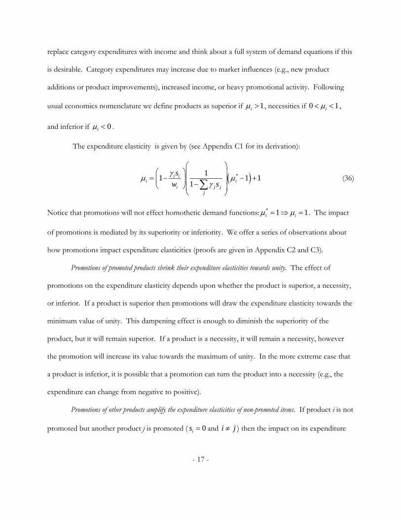
The expenditure elasticity is given by (see Appendix C1 for its derivation):
*11 1 1
1i i
i ii j j
j
s
w s
(36)
Notice that promotions will not effect homothetic demand functions: * 1 1i i . The impact
of promotions is mediated by its superiority or inferiority. We offer a series of observations about
how promotions impact expenditure elasticities (proofs are given in Appendix C2 and C3).
Promotions of promoted products shrink their expenditure elasticities towards unity. The effect of
promotions on the expenditure elasticity depends upon whether the product is superior, a necessity,
or inferior. If a product is superior then promotions will draw the expenditure elasticity towards the
minimum value of unity. This dampening effect is enough to diminish the superiority of the
product, but it will remain superior. If a product is a necessity, it will remain a necessity, however
the promotion will increase its value towards the maximum of unity. In the more extreme case that
a product is inferior, it is possible that a promotion can turn the product into a necessity (e.g., the
expenditure can change from negative to positive).
Promotions of other products amplify the expenditure elasticities of non-promoted items. If product i is not
promoted but another product j is promoted ( 0is and i j ) then the impact on its expenditure
- 18 -
elasticity depends upon its position in the market. If the product is superior, * 1i , then it will
become more superior: * 1i i . If the product is inferior, * 1i , then it will become more
inferior: * 1i i . Potentially, it can even push a product that was considered a necessity to
become inferior. For example, suppose there are two products and the first product is the market
leader (e.g., high market share: 1 .9w , superior: *1 1.2 , and promotions have a strong positive
influence: 1 .5 ), then the promotion of the market leader can make the non-promoted product
move from necessary ( *2 .2 ) to inferior ( *
1 .6 ). In summary, strong products can benefit
from competitor promotions, while weak products are hurt.
Promotions that expand the consumer base will benefit superior products. If promotions simply
reallocate share across products within the category, then promotions will clearly result in a loss of
market share for non-promoted products. As discussed in section 2 we know that if product i is not
promoted that *i iw w . However, it is possible that promotions may bring new consumers and
increase expenditures in a product category. The marginal increase of an additional dollar of
expenditures will be allocated proportional to the expenditure elasticities. Hence, promotions can
benefit strong products within a category through increased quantity sales.
3.2 Price Elasticities
A common measure of price competition is through the measure of price elasticities.
Uncompensated price elasticities ( ij ) measure the effect of a change in the Marshallian demand of
product i from a change in the price of product j: jiij
j i
pq
p q
. Compensated elasticities ( ij )
- 19 -
similarly measure the effect of a change in the Hicksian demand of product i from a change in the
price of product j:
0
jiij
j i u u
pq
p q
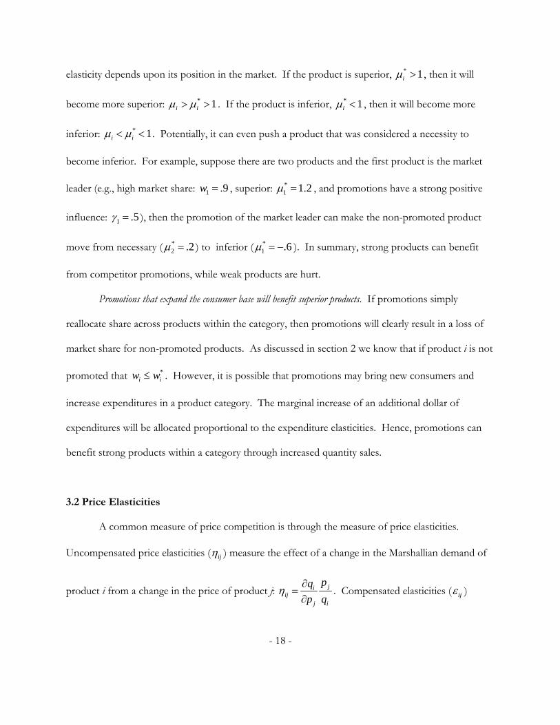
. The uncompensated own-price elasticities of our modified
system in terms of the original system are:
*
*
1 1 1 1 if
1 1 if
i iij j j i
i
ij
i iij j j i
i
ss i j
w
ss i j
w
(37)
The uncompensated cross-price elasticities are:
*
*
1 1 1 if
1
1 if
1
j j ji ii iij j
i ik k
k
ij
j j ji ii iij j
i ik k
k
w sw ssw i j
w ws
w sw ssw i j
w ws
(38)
We refer the reader to Appendix C4 and C5 for the derivation of these equations and proofs of the
statements that follow.
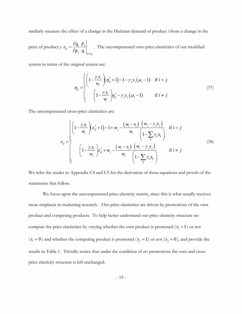
We focus upon the uncompensated price elasticity matrix, since this is what usually receives
more emphasis in marketing research. Our price elasticities are driven by promotions of the own
product and competing products. To help better understand our price elasticity structure we
compute the price elasticities by varying whether the own product is promoted ( 1is ) or not
( 0is ) and whether the competing product is promoted ( 1js ) or not ( 0js ), and provide the
results in Table 1. Trivially notice that under the condition of no promotions the own and cross
price elasticity structure is left unchanged.
- 20 -
Own Promotion
Competitor Promotion
Yes ( 1is ) No ( 0is )
Own-Price Elasticities ( i j )
Yes ( 1js ) *1 1 1 1iii i i
iw
*ii
No ( 0js )
Cross-Price Elasticities ( i j )
Yes ( 1js ) *1 1iij j i
iw
* 1ij j i
No ( 0js ) *1 iij
iw
*ij
Table 1. Uncompensated Cross Price Elasticity Matrix under varying own and cross promotions.
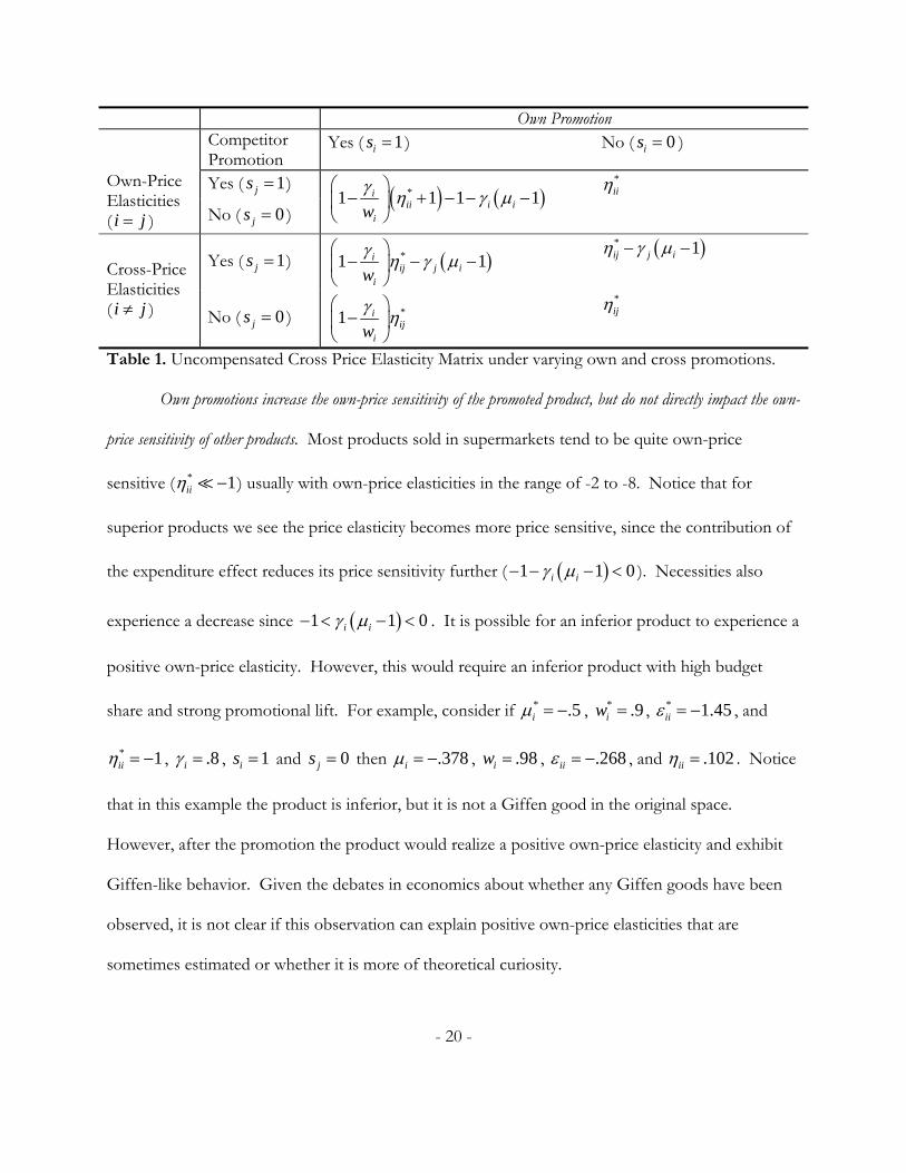
Own promotions increase the own-price sensitivity of the promoted product, but do not directly impact the own-
price sensitivity of other products. Most products sold in supermarkets tend to be quite own-price
sensitive ( * 1ii ) usually with own-price elasticities in the range of -2 to -8. Notice that for
superior products we see the price elasticity becomes more price sensitive, since the contribution of
the expenditure effect reduces its price sensitivity further ( 1 1 0i i ). Necessities also
experience a decrease since 1 1 0i i . It is possible for an inferior product to experience a
positive own-price elasticity. However, this would require an inferior product with high budget
share and strong promotional lift. For example, consider if * .5i , * .9iw , * 1.45ii , and
* 1ii , .8i , 1is and 0js then .378i , .98iw , .268ii , and .102ii . Notice
that in this example the product is inferior, but it is not a Giffen good in the original space.
However, after the promotion the product would realize a positive own-price elasticity and exhibit
Giffen-like behavior. Given the debates in economics about whether any Giffen goods have been
observed, it is not clear if this observation can explain positive own-price elasticities that are
sometimes estimated or whether it is more of theoretical curiosity.
- 21 -
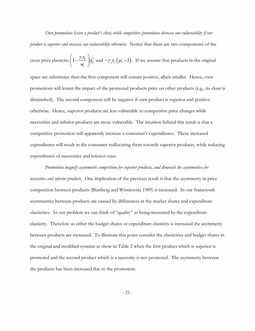
Own promotions lessen a product’s clout, while competitive promotions decrease our vulnerability if our
product is superior and increase our vulnerability otherwise. Notice that there are two components of the
cross price elasticity: *1 i iij
i
s
w
and 1j j is . If we assume that products in the original
space are substitutes then the first component will remain positive, albeit smaller. Hence, own
promotions will lessen the impact of the promoted products price on other products (e.g., its clout is
diminished). The second component will be negative if own product is superior and positive
otherwise. Hence, superior products are less vulnerable to competitive price changes while
necessities and inferior products are more vulnerable. The intuition behind this result is that a
competitive promotion will apparently increase a consumer’s expenditures. These increased
expenditures will result in the consumer reallocating them towards superior products, while reducing
expenditures of necessities and inferior ones.
Promotions magnify asymmetric competition for superior products, and diminish the asymmetries for
necessities and inferior products. One implication of the previous result is that the asymmetry in price
competition between products (Blattberg and Wisniewski 1989) is increased. In our framework
asymmetries between products are caused by differences in the market shares and expenditure
elasticities. In our problem we can think of “quality” as being measured by the expenditure
elasticity. Therefore as either the budget shares or expenditure elasticity is increased the asymmetry
between products are increased. To illustrate this point consider the elasticities and budget shares in
the original and modified systems as show in Table 2 when the first product which is superior is
promoted and the second product which is a necessity is not promoted. The asymmetry between
the products has been increased due to the promotion.

- 22 -
Product
Market Share
Expenditure Elasticities
Compensated Elasticity
Uncompensated Elasticity
1 2 1 2 Original 1 .60 1.2 -2.02 2.02 -2.74 1.54
2 .40 0.7 3.02 3.02 2.60 -3.30 Modified 1 .80 1.15 -.81 .81 -1.73 .58
2 .20 0.4 3.22 -3.22 2.90 -3.30 Table 2. Example to illustrate increased asymmetry for two products system ( 1
1 2 2 ). The first product is promoted and a superior, while the second is not promoted and a necessity. To illustrate what happens when the first product is not promoted while the second product
is promoted consider the results given in Table 3. Notice that the promotion of the weaker product
has result in an increase in its share, a decrease in its own-price sensitivity, and a reduction in the
vulnerability of price changes to the first product. In summary, the asymmetry between the
products has been reversed.
Product
Market Share
Expenditure Elasticities
Compensated Elasticity
Uncompensated Elasticity
1 2 1 2 Original 1 .60 1.2 -2.02 2.02 -2.74 1.54
2 .40 0.7 3.02 -3.02 2.60 -3.30 Modified 1 .30 1.4 -2.32 2.32 -2.74 1.34
2 .70 0.83 .99 -.99 .74 -1.57 Table 3. Example to illustrate increased asymmetry for two products system ( 1
1 2 2 ). The first product is promoted and a necessity, while the second is not promoted and superior. Competitive promotions can result in sign-reversal for cross-price elasticities. A vexing problem for
applied researchers is negative cross-price elasticities. In general products within a category are
assumed to be substitutes, which means that the cross price elasticities should be small positive
numbers. One explanation is that these negative cross-price elasticities can result from the second
component, 1j j is , in equation (37). Notice that if the promotional effect of the competing
product j is strong and the superiority of product i is high, then apparent substitutes can become
complements. Consider another example in Table 4, where the first product is strongly superior but
- 23 -
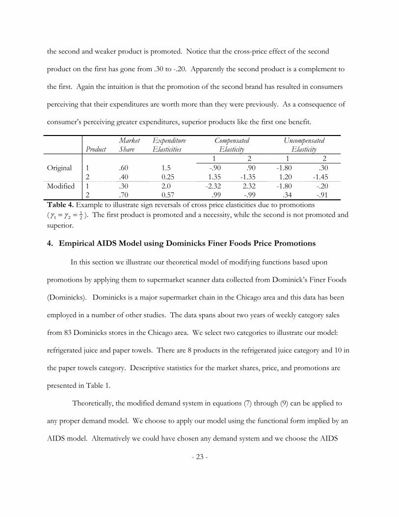
the second and weaker product is promoted. Notice that the cross-price effect of the second
product on the first has gone from .30 to -.20. Apparently the second product is a complement to
the first. Again the intuition is that the promotion of the second brand has resulted in consumers
perceiving that their expenditures are worth more than they were previously. As a consequence of
consumer’s perceiving greater expenditures, superior products like the first one benefit.
Product
Market Share
Expenditure Elasticities
Compensated Elasticity
Uncompensated Elasticity
1 2 1 2 Original 1 .60 1.5 -.90 .90 -1.80 .30
2 .40 0.25 1.35 -1.35 1.20 -1.45 Modified 1 .30 2.0 -2.32 2.32 -1.80 -.20
2 .70 0.57 .99 -.99 .34 -.91 Table 4. Example to illustrate sign reversals of cross price elasticities due to promotions ( 1
1 2 2 ). The first product is promoted and a necessity, while the second is not promoted and superior. 4. Empirical AIDS Model using Dominicks Finer Foods Price Promotions
In this section we illustrate our theoretical model of modifying functions based upon
promotions by applying them to supermarket scanner data collected from Dominick’s Finer Foods
(Dominicks). Dominicks is a major supermarket chain in the Chicago area and this data has been
employed in a number of other studies. The data spans about two years of weekly category sales
from 83 Dominicks stores in the Chicago area. We select two categories to illustrate our model:
refrigerated juice and paper towels. There are 8 products in the refrigerated juice category and 10 in
the paper towels category. Descriptive statistics for the market shares, price, and promotions are
presented in Table 1.
Theoretically, the modified demand system in equations (7) through (9) can be applied to
any proper demand model. We choose to apply our model using the functional form implied by an
AIDS model. Alternatively we could have chosen any demand system and we choose the AIDS

- 24 -
models since it is theoretically consistent and has been employed both other researchers using
scanner data. Up to this point we have not discussed that promotions may take different forms in
supermarket environments. The two predominate forms are feature promotions and display
promotions. Feature promotions or more simply features refer to out of store advertisements that
are placed in printed weekly circulars that are distributed to households directly or in-store or
sometimes features are simultaneously promoted via television or radio. Display promotions or
more simply displays refer to in-store advertisements that are placed next to the product. For
example, in the Dominicks dataset displays may include signs displaying the text “bonus buy”, shelf-
talkers, coupon dispensers, large end-of-aisle displays, or other types of special in-store promotional
displays (e.g., cardboard cutouts in front of the product).
To account for these two types of promotions we augment our model to think of
promotions as a vector. In our notation is becomes i i if ds , where if is feature and id is
display for product i. The scalar effects in our model now become dot products, i is becomes
f di i i i if d γ s and i is becomes f d
i i i i if d β s . Our modifying functions are easily
generalized except that our restrictions in equation (6) becomes 0 1i ii
γ s . Again since our
indicators only take values on the unit interval we enforce the following sufficient conditions:
0 1, 0 1, 0 1, 0 1f d f d f di i i i i i
i
(39)
Following others who have worked with this data we aggregate individual products that are
promoted together (e.g., plain white versus printed patterns, scented versus unscented, or orange
juice with pulp versus without) and our promotion indicators become indices that are weighted by
individual product sales.

- 25 -
Using the introduction of display and feature promotions we postulate the form of our
AIDS model that we employ in our empirical application follows from equations (34) and (35) given
in section 2.3. We model the expected market share ( iktw ) for product i in store k at week t:
1 1
1 ln( / ) 1 ln( )M M
ikt ik ikt jk jkt ik ik kt kt jk jkt ijk jkt jk jktj j j
w x P p
γ s γ s γ s β s (40)
Where ktP is a price index defined by:
10 2
ln( ) ln( ) 1
ln( ) ln( ) ln( )
kt jk jkt jkt jk jktj j
k jk jkt jk jkt jlk jkt jk jkt lkt lk lktj j l
P p
p p p
γ s γ s
β s β s β s
(41)
Throughout this paper we have assumed that economic theory holds, therefore we also enforce the
restrictions implied by adding up, homogeneity, and symmetry from equations (29), (30), and (31),
respectively. We refer to this as model A.
We assume that these restrictions hold exactly. However, if we so desired we could follow
Montgomery and Rossi (1999) and use these restrictions as prior information over which we center
our data. Our reasoning for not attempting to relax these restrictions is that we are attempting to
see what economic theory has to offer, and it is outside the scope of this paper to test whether
economic theory holds.
An alternative model B is to assume that the promotional patterns are nullified in which case
we are left with the standard AIDS model:
ln( / ) ln( )ikt ik ik kt kt ijk jktj
w x P p (42)
Where ktP is a price index defined by:
- 26 -
10 2ln( ) ln( ) ln( ) ln( )kt k j jkt jlk jkt lkt
j j l
P p p p (43)
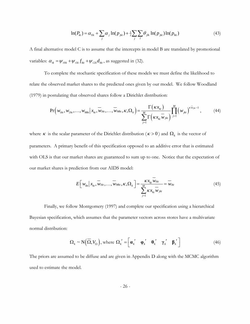
A final alternative model C is to assume that the intercepts in model B are translated by promotional
variables: 0 1 2ik i k i k ikt i k iktf d , as suggested in (32).
To complete the stochastic specification of these models we must define the likelihood to
relate the observed market shares to the predicted ones given by our model. We follow Woodland
(1979) in postulating that observed shares follow a Dirichlet distribution:
1
11 21
1
Pr , , , , , , , ,jkt
M wktkt Mktkt kt Mkt kt k jktM
jjktkt
j
xw w w x w w w
x w
, (44)
where is the scalar parameter of the Dirichlet distribution ( 0 ) and k is the vector of
parameters. A primary benefit of this specification opposed to an additive error that is estimated
with OLS is that our market shares are guaranteed to sum up to one. Notice that the expectation of
our market shares is prediction from our AIDS model:
1
1
, , , , ,iktkt
kt Mkt iktikt kt k M
jktktj
x wE w x w w w
x w
(45)
Finally, we follow Montgomery (1997) and complete our specification using a hierarchical
Bayesian specification, which assumes that the parameter vectors across stores have a multivariate
normal distribution:
~ N ,k V , where k k k k k k α φ θ γ β (46)
The priors are assumed to be diffuse and are given in Appendix D along with the MCMC algorithm
used to estimate the model.

- 27 -
5. Findings from Empirical Estimates of AIDS Model using Dominicks Data
[discuss results, the key point is to reinforce the findings from the analytical section to the
extent that they are present]
6. Discussion and Conclusions
Economic theory is criticized for making unrealistic assumptions about consumer behavior.
However, instead of positing a new theory of consumer behavior we have returned to the classical
economic approach. This is driven by our belief that economic theory is a powerful device for
understanding consumer behavior. It is beyond the scope of this research to prove whether the
economic approach is correct. Instead we have simply asked what insights it has to offer about
promotions if they operate within standard economic theory. Our desire to rely upon theory is not
meant to be an affront to empirical approaches to understanding how promotions work (Blattberg,
Briesch and Fox 1995, van Heerde et al 2002), since empirical analysis generalizations can offer
insights to both practice and theory.
We have introduced promotional effects so that they interact with price and expenditures.
Central to our approach is the premise that promotions may affect customer perceptions of prices,
expenditure, and products, and temporarily alter the consumer decision-making process. Our
theoretical framework is based upon the work of Lewbel (1985) to demonstrate how promotions
can be incorporated into demand systems using modifying functions. Ours is the first within
marketing to suggest such an approach. A primary advantage of this approach is that it yields a
regular method for incorporating promotions into any demand system. Theoretically we have

- 28 -
shown that perceptual changes of prices and expenditures are consistent with classical economic
theory. An alternative interpretation of our modifying functions is that they posit the existing of
intermediary or shadow goods that enter into a consumer’s utility maximization or cost
minimization problems. However, the essence of the classical economic approach remains intact.
Our results show that promotions moderate substitution between products. We
demonstrate both analytically and numerically a number of findings that we believe are of theoretical
and practical importance for empirical research on price promotions. The main effect of
promotions is that they increase market share. However, there are many other more subtle effects
that depend upon the strength of the product. For example, as the category expands we find that
superior products can benefit from promotions over weaker ones. The vulnerability of a product to
competitor prices can be lessened if it is superior, while lesser products will experience increased
price competition. The often discussed asymmetric competition between products can either be
magnified or reduced by promotions. If promotional effects are strong enough then substitution
between a promoted product and superior alternative can be depressed enough that we can see sign
reversals in the cross-price elasticity between this promoted product and its non-promoted superior-
alternative. Negative cross-price elasticities are persistent problems when estimating demand models
in marketing applications, and promotions may provide an explanation for why these unexpected
signs can occur for apparent substitutes.
A limitation of our current research is that we consider only one family of modifying
functions. This family was motivated by our desire to translate demand and to introduce a simple
scaling function of prices. However, it is not a unique solution to the problem. There may exist
other modifying functions that better capture consumer behavior. We hope our work encourages
other to consider the use of modifying functions in understanding how promotions impact demand.
- 29 -
References
Allenby, Gregory M. and Peter E. Rossi (1991), “Quality Perceptions and Asymmetric Switching Between Brands”, Marketing Science, 10 (3), 185-204.
Blattberg, Robert C., Richard Briesch, and Edward J. Fox (1995), “How Promotions Work”, Marketing Science, 14 (3), G122-G132.
Blattberg, Robert C. and Scott A. Neslin (1990), Sales Promotion: Concepts, Methods, and Strategies, Englewood Cliff, NJ: Prentice Hall.
Blattberg, Robert C. and Kenneth J. Wisniewski (1989), “Price-Induced Patterns of Competition”, Marketing Science, 8 (4), 291-309.
Cotterill, Ronald W., William P. Putsis, Jr., and Ravi Dhar (2000), Assessing the Competitve Interaction between Private Labels and National Brands”, Journal of Business, 73 (1), 109-137.
Deaton, Angus and John Muellbauer (1980), “An Almost Ideal Demand System”, American Economic Review, 70, 312-326.
Dickson, Peter R. and Alan G. Sawyer (1990), “The Price Knowledge and Search of Supermarket Shoppers”, Journal of Marketing, 54, 42-53.
Dreze, Xavier, Patricia Nisol, and Naufel J. Vilcassim (2004), “Do Promotions Increase Store Expendtirue?” A Descriptive Study of Household Shopping Behavior”, Quantitative Marketing and Economics, 2, 59-92.
Guadagni, Peter M. and John D.C. Little (1983), “A Logit Model of Brand Choice Calibrated on Scanner Data”, Marketing Science, 27 (1), 29-48.
Heilman, Carrie M., Kent Nakamoto, and Ambar Rao (2002), “Please Surprises: Consumer Respond to Unexepcted In-Store Coupons”, Journal of Marketing Research, 39, 242-252.
Inman, J. Jeffrey, Leigh McAlister, and Wayne D. Hoyer (1990), “Promotion Signal: Proxy for a Price Cut?”, Journal of Consumer Research, 17, 74-81.
Lattin, James M. and Randolph E. Bucklin (1989), “Reference Effects of Price and Promotionon Brand Choice Behavior”, Journal of Marketing Research, 26, 299-309.
Lewbel, Arthur (1985), “A Unified Approach to Incorporating Demographic of Other Effects into Demand Systems”, Review of Economic Studies, 52 (1), 1-18.
Montgomery, Alan L. (1997), “Creating Micro-Marketing Pricing Strategies Using Supermarket Scanner Data”, Marketing Science, 16 (4), 315-337.
Montgomery, Alan L. and Peter E. Rossi (1999), “Estimating Price Elasticities with Theory-based Priors”, Journal of Marketing Research, 36 (4), 413-423.
Mulhern, Francis J. and Daniel Padgett (1995), “The Relationship Between Retail Price Promotions and Regular Price Purchases”, Journal of Marketing, 59, 83-90.
Putsis and Cotterill 2001
- 30 -
van Heerde, Harald J., Peter S. H. Leeflang, and Dick R. Wittink (2002), “How Promotions Work: SCAN*PRO-Based Evolutionary Model Building”, Schmalenbach Business Review (54), 198-220.
Wittink, Dick R., M. J. Addona, W.J. Hawkes, and J.C. Porter (1988), “SCAN*PRO: The Estimation, Validation and Use of Promotion Effects Based on Scanner Data”, Cornell University, Working Paper.
Woodland, A. D. (1979), “Stochastic Specification and the Estimation of Share Equations”, Journal of Econometrics, 10, 361-383.

- Appendix 1 -
Appendix A: Consistency of our Modifying Functions
A1. Consistency of General Functional Form
We show the consistency of the general form of our modifying functions by verifying that they
satisfy Theorems 1, 2, and 3 of Lewbel (1985). First we restate our modifying definitions from
equations (10) and (11):
* * ( ) ( )( , , ) ( ) ( , )f m m m P d dp d d p d , where 1
( , ) i
nd
ii
P p
p d
* ( ) ( , ) ( ) ;i i i ih p p dp d d
Compliance with Lewbel's Theorem 1:
( )
* * ( )
* ( ) ( )
1
*
*
( ) ( )( , ) ( ) ( , );
( )
( )
1 1 1 ;
( ) ( )( , ) ( , ) ( ) ( );
( ) ( )
1 ( ).
i
ji i i i i
j j i i i i i
nd
j ij j i
jj jj
jj
ph h p p
p p p p p
d m ppf
dp f f
f m
m f
d
d
d
d d
d dp d d p d
d
d
d dp d p d d d
d d
d
Compliance with Lewbel's Theorem 2:
*( ) ( , , ) 0 ( ) 0;a f m p d d
*
( )( ) 0 0;
( )
fb
m
d
d
( ) 0 0;ii
fc d
p
- Appendix 2 -
( ) for all and , 0 ( ) ( ) 0 ;ji
i
hd i j
p
d d
( ) at least one ( ) 0ie d
Compliance with Lewbel's Theorem 3:
2
2
2
2
2
2
( , , ) ( ) ( ) ( )0 1 0 1
( ) ( ) ( )
( , , )0 ( 1) 0 1
( , )( )[ (0 ) 1] 0
i i ij
i
j
f m
m
f md d d
p
h
p
p d d d d
d d
d
d
d
pd
p
d
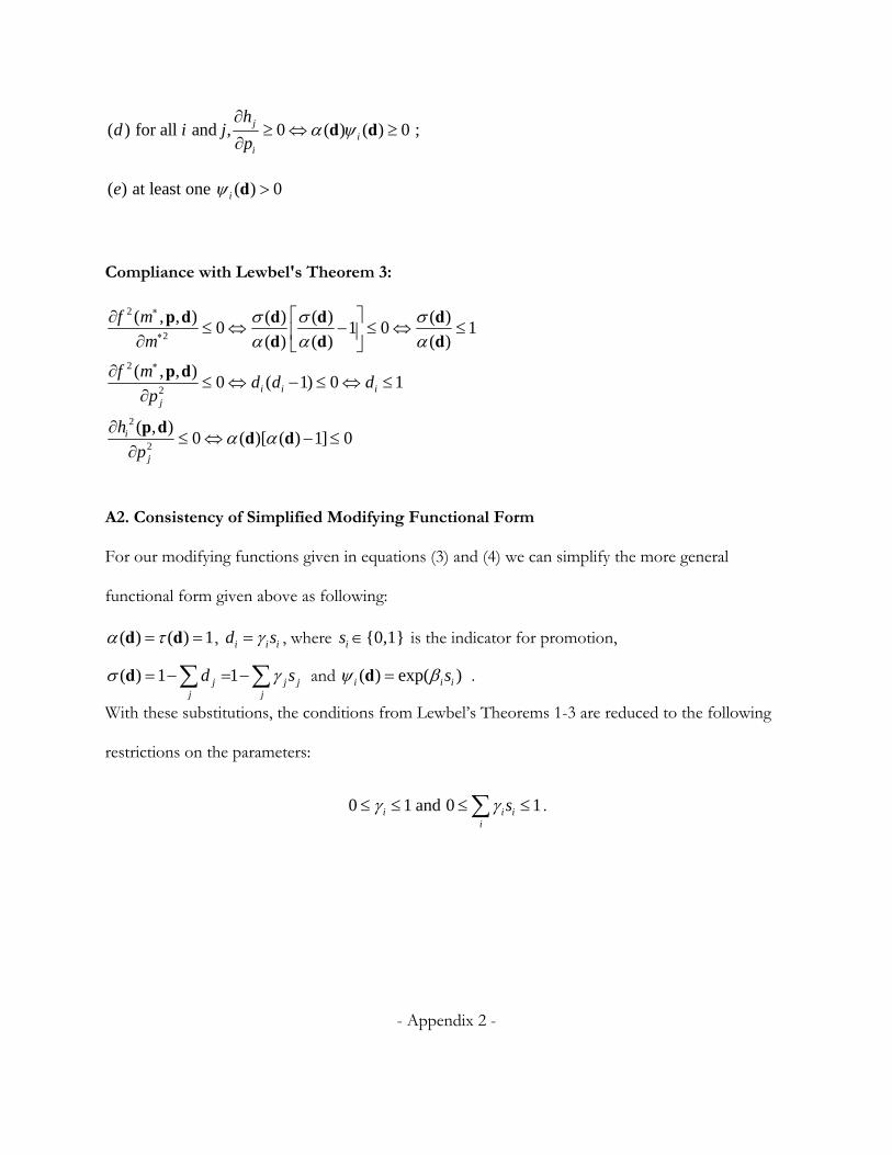
A2. Consistency of Simplified Modifying Functional Form
For our modifying functions given in equations (3) and (4) we can simplify the more general
functional form given above as following:
( ) ( ) 1 d d , i i id s , where {0,1}is is the indicator for promotion,
( ) 1 1 j j jj j
d s d and ( ) exp( ) i i is d .
With these substitutions, the conditions from Lewbel’s Theorems 1-3 are reduced to the following
restrictions on the parameters:
0 1 and 0 1i i ii
s .

- Appendix 3 -
Appendix B: Cobb-Douglas Demand Example
First, we provide some definitions and their specifications that we shall use or prove in this
appendix:
Direct utility: 1/2 1/21 2( ) ,u q q q s.t. 1 1 2 2p q p q m
Marshallian Demand: 11
;2
mq
p
22
;2
mq
p
Indirect Utility: 1 2 1 2
1
2 2 2
m m mu
p p p p
Cost Function: 1 22m u p p
Hicksian Demand: ( 1/2) 1/21 1 2 ;q up p 1/2 ( 1/2)
2 1 2q up p
Market Share: 1 11 1
1
1;
2 2
p qmq w
p m
2
1.
2w
B1. Derivation of Demand Model Using Cobb-Douglas Utility
Utility Maximization Subject to a Budget Constraint
We start with a Cobb-Douglas utility specification for two brands, 1/2 1/2i ju q q . The budget
constraint is i i j jm p q p q . Hence, our utility maximization problem is:
1 2
1/2 1/21 2 1 1 2 2
,max , s.t. q q
U m pq qq p q
We formulate the Lagrangean that is associated with our problem:
1/2 1/21 2 1 1 2 2( )m p q p qq q

- Appendix 4 -
The first order conditions for this optimization problem are met when:
1/2 1/2 1/2 1/2
1/2 1/2 1/2
1 2 1 1 2 11
1 2 2 1 2 22
2 1 2 2 1 11 1 2 2 1 2
1 2 1
1/2
2
1 0 ;2
1 0 ;2
0; , or a
12
1
nd ;
2
pq
pq
q p p q p qm p q p q q q
q
q q q q p
q q q q p
p p p
Hence, 2 2 2 2 1 1 1 11 2
1 1 2 2
and m p q p q m p q p q
q qp p p p
, which yields the optimum solution:
1 21 2
; .2 2
m mq q
p p
Cost Minimization Subject to Utility Constraint
The dual of our previous utility maximization problem is to minimize our expenditures
subject to a utility constraint:
1 1 21/2
2 112/2min{ }, s.t. = ,p q p q q qu
Which yields the Lagrangean:
1 1 2 2 1 21/2 1/2( )p q p qq u q
The first order conditions imply the following:
1/2 1/2 1/2 1/2
1/2 1/2 1/2 1/2
1
1 1 2 1 1 21
2 1 2 2 1 22
1 2 21 2 1
2
/2 1/2 2
1 1
1 10 ;2 2
1 10 ;2 2
0; , or ;
q q q q
q q q q
qq q
q
p u p uq
p u p uq
p p qu q
p p

- Appendix 5 -
Hence 22
1
=p
u qp
and 11
2
=p
u qp
which yields the Hicksian demand functions:
1/2 1/21 1 2q up p and 1/2 1/2
2 1 2q up p .
B2. Demand for Modified Cobb-Douglas Utility Model
In this section we deduce the demand models for the Cobb-Douglas Utility with our
modifying functions using Lewbel’s Theorems and directly through substitution and optimization.
Deduction of Demand using Lewbel’s Theorems
First we restate our modifying functions for price and expenditures:
( ), exp( )i i i i i ip h p s p s ;
(1 ) *(11
)
1
, or / , i i i i i i
ns s s
ii
p m mm m P P P
The derivatives of these transformations are:
(1 )*
*
*
exp( ), if
0, if
(1 )
j j
j j
i ii
j
s i i
i i
sj j
j
s i jh
i jp
sfm P
p p
fs m P
m
Following Lewbel the indirect utility can be found by equating the indirect utility from the original
system through substitution:
- Appendix 6 -
1 1 2 2(11
** * *
* *1 1 1 2 21
)
22
/( , ,
exp( )) ( ,
exp( ))
22
s sm PmV m p
p s pr m p
p p sV
We can derive the Hicksian Demand using Lewbel’s Theorem 4:
( ) (1 )(1 ) exp( )j j j js si i ii i j j i i i
i i i
h sf fq q s m P s q m P
m p p p
( ) (1 )( 1/2) (1/2)(1 ) exp( )j j j js s i ij j i i i j
i
ss m P s up p m P
p
( ) exp( )(1 )exp( )
exp( )j js j j j i i
j j i ii i i i
p s sm P s s u m
p s p
( ) exp( )2 (1 )exp( ) 2
exp( )
j jsj j j i i
i j j j i i i ji i i i
p s su p p P s s u u p p
p s p
( ) 12 exp( ) (1 )exp( ) 2 exp( )
exp( )
j jsi i
i j j j j j j i i i i ii i i i
su p p Pu p s s s p s
p s p
( ) 12 exp( ) exp( ) (1 ) 2
j js
i j j j j i i i j j i ii
u p p Pu p s p s s sp
(1 )( )2 exp( ) exp( ) (1 )j j
j jss
i i i j j j i i j ji
Pu p s p s s s
p
The Marshallian demand can be found following the same theorem:
( ) (1 )(1 ) exp( )2
j j j js si i ii i j j i i
i i i i
h sf f mq q s m P s m P
m p p p p
(1 ) 1(1 )exp( )
2j js i i
j j i ii i
sm P s s
p p
(1 ) 1 1
(1 ) (1 )2 2
j jsj j i i j j i i
i i
P mm s s s s
p p
- Appendix 7 -
(1 )2 i i j j
i
ms s
p
Finally, we can compute the budget shares:
1(1 )
2i i
i i i j j
q pw s s
m
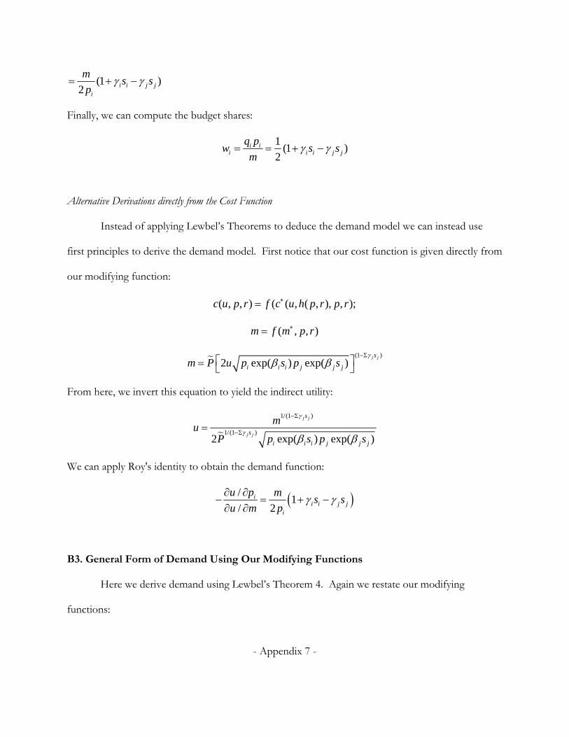
Alternative Derivations directly from the Cost Function
Instead of applying Lewbel’s Theorems to deduce the demand model we can instead use
first principles to derive the demand model. First notice that our cost function is given directly from
our modifying function:
( , , ) ( ( , ( , ), , );c u p r f c u h p r p r
( , , )m f m p r
(1 )
2 exp( ) exp( )j js
i i i j j jm P u p s p s
From here, we invert this equation to yield the indirect utility:
1/(1 )
1/(1 )2 exp( ) exp( )
j j
j j
s
s
i i i j j j
mu
P p s p s
We can apply Roy's identity to obtain the demand function:
/1
/ 2i
i i j ji
u p ms s
u m p
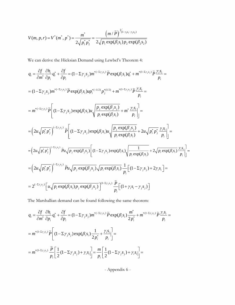
B3. General Form of Demand Using Our Modifying Functions
Here we derive demand using Lewbel’s Theorem 4. Again we restate our modifying
functions:
- Appendix 8 -
exp( )i i i ip p s
1
1( / ) ,j jsm m P 1
j j
ns
jj
P p
(1 )j jsm m P
Marshallian demand is:
( ) (1 )(1 ) exp( )j j j js si i ii i j j i i i
i i i
h sf fq q s m P s q m P
m p p p
(1 ) 1 1(1 ) exp( )
(1 )j js i i
j j i i ii j j
ss m P m s q
p s
(1 )(1 )
i i i ij j
i j j
q p sms
p m s
(1 ) (1 )(1 )
i ii j j i j j i i i
j j
sw s w s w s
s
Market share is:
(1 )(1 )(1 )
j j
j j
ssi i i i i i
i i j j ii i i i
h p p s pf m f m Pw w s w m P
m m p p p m m p m
(1 )i j j i i iw s w s
Hicksian demand is:
( ) (1 )ˆ ˆ (1 ) exp( )j j j js si i ii i j j i i i
i i i
h sf fq q s m P s q m P
m p p p
(1 ) ˆ 1(1 ) exp( )
(1 )j js i i i
j j i ii j j
q ss m P s
m p s
- Appendix 9 -
1
1
exp( )ˆ(1 )
( / ) j j
i i i ij j i
is
m s ss q m
pm P
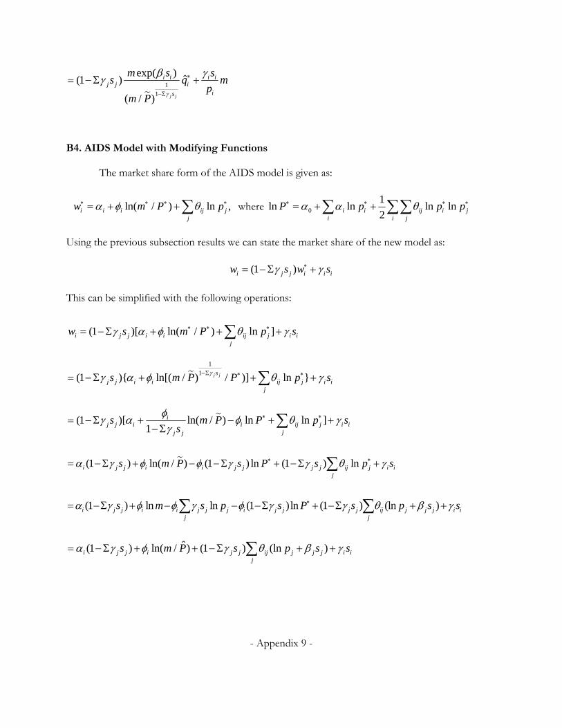
B4. AIDS Model with Modifying Functions
The market share form of the AIDS model is given as:
ln( / ) ln ,i i i ij jj
w m P p where 0
1ln ln ln ln
2i i ij i ji i j
P p p p
Using the previous subsection results we can state the market share of the new model as:
(1 )i j j i i iw s w s
This can be simplified with the following operations:
(1 )[ ln( / ) ]lni j j i i j j ij
i iw s m P p s
1
1(1 ){ ln[( / ) / )] ln }j jsj j i i ij j i i
j
s m P P p s
(1 )[ ln( / ) ln l1
]nij j i i ij j i i
j j j
s m P P p ss
(1 ) ln( / ) (1 ) ln (1 ) lni j j i i j j j j ij j i ij
s m P s P s p s
(1 ) ln ln (1 )ln (1 ) (ln )i j j i i j j j i j j j j ij j j j ijj
is m s p s P s p s s
ˆ(1 ) ln( / ) (1 ) (ln )i j j i j j ij j j j i ij
s m P s p s s

- Appendix 10 -
where ˆln ln (1 ) lnj j j j jj
P s p s P and
0
1ln (ln ) (ln )(ln )
2i i i i ij i i i j j ji i j
P p s p s p s
Notice that the price index of this new modifying form is an average of a price index based upon
promoted prices and the original price index with modified prices.
- Appendix 11 -
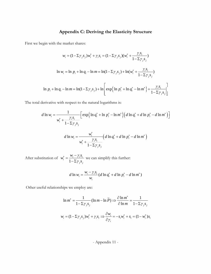
Appendix C: Deriving the Elasticity Structure
First we begin with the market shares:
(1 ) (1 )( )1
i ii j j i i i j j i
j j
sw s w s s w
s
ln ln ln ln ln(1 ) ln( )1
i ii i i j j i
j j
sw p q m s w
s
ln ln ln ln(1 ) ln exp ln ln ln1
i ii i j j i i
j j
sp q m s p q m
s
The total derivative with respect to the natural logarithms is:
1ln exp ln ln ln ln ln ln
1
i i i i ii i
ij j
d w q p m d q d p d ms
ws
ln ln ln ln
1
ii i i
i ii
j j
wd w d q d p d m
sw
s
After substitution of 1
i i ii
j j
w sw
s
we can simplify this further:
ln ( ln ln ln )i i ii i i
i
w sd w d q d p d m
w
Other useful relationships we employ are:
1 ln 1ln (ln ln )
1 ln 1j j j j
mm m P
s m s
(1 ) (1 )ii j j i i i i i i i i
i
ww s w s s w s w s
- Appendix 12 -
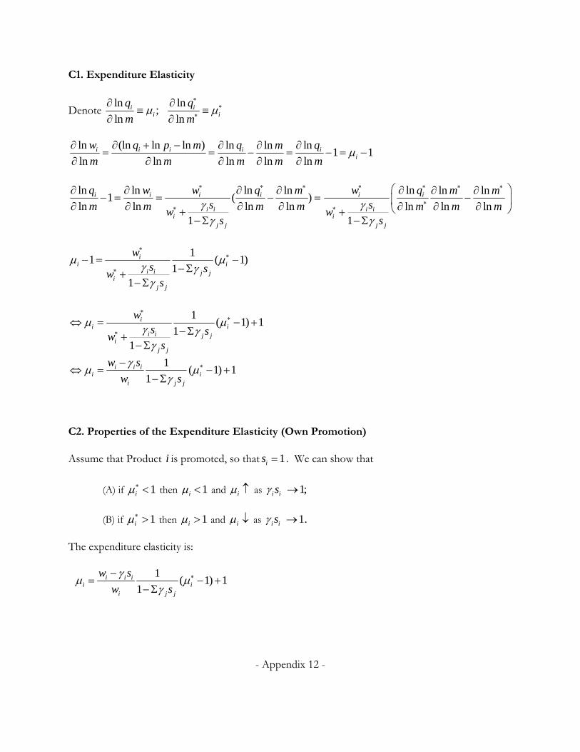
C1. Expenditure Elasticity
Denote ln
;ln
ii
q
m
ln
lni
i
q
m
ln (ln ln ln ) ln lnln1 1
ln ln ln ln lni i i i i
i
w q p m q qm
m m m m m
ln ln ln ln1 ( )
ln ln ln ln1
i i i i
i ii
j j
q w w q msm m m mw
s
ln ln ln
ln ln ln1
i i
i ii
j j
w q m ms m m mw
s
11 ( 1)
11
ii i
i i j ji
j j
ws sw
s
1( 1) 1
1i i i
i ii j j
w s
w s
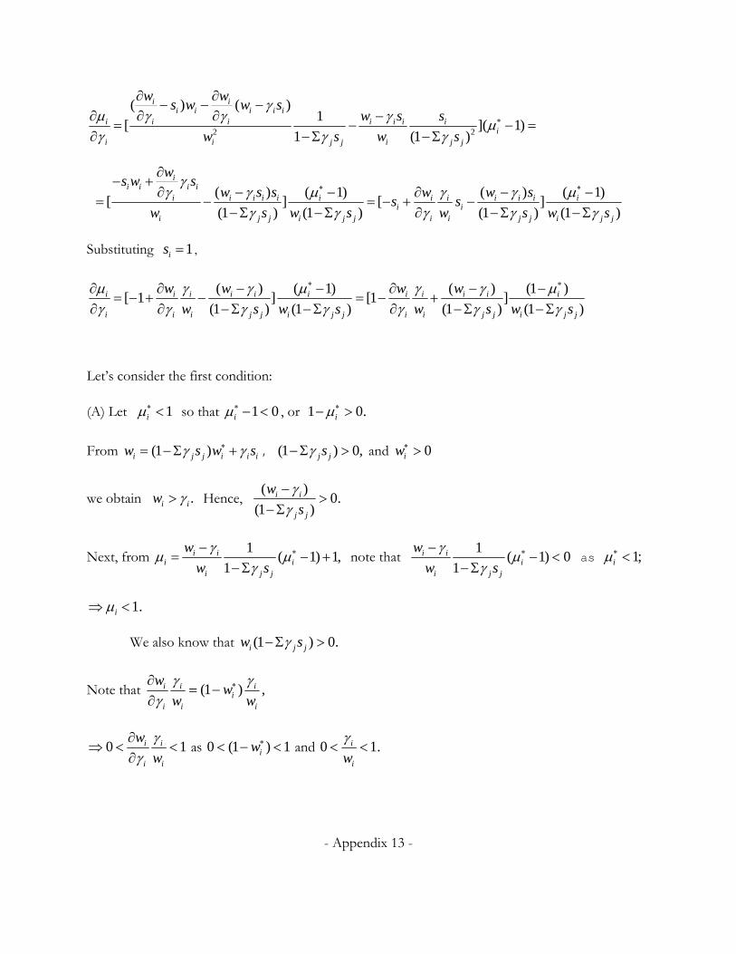
C2. Properties of the Expenditure Elasticity (Own Promotion)
Assume that Product i is promoted, so that 1is . We can show that
(A) if 1i then 1i and i as i is 1;
(B) if 1i then 1i and i as i is 1.
The expenditure elasticity is:
1
( 1) 11
i i ii i
i j j
w s
w s
1( 1) 1
11
ii i
i i j ji
j j
ws sw
s
- Appendix 13 -
2 2
( ) ( )1
[ ]( 1)1 (1 )
i ii i i i i
i i i i i i ii
i i j j i j j
w ws w w s
w s s
w s w s
( ) ( 1) ( ) ( 1)
[ ] [ ](1 ) (1 ) (1 ) (1 )
ii i i i
i i i i i i i i i i i ii i
i j j i j j i i j j i j j
ws w s
w s s w w ss s
w s w s w s w s
Substituting 1is ,
( ) ( 1) ( ) (1 )[ 1 ] [1 ]
(1 ) (1 ) (1 ) (1 )i i i i i i i i i i i
i i i j j i j j i i j j i j j
w w w w
w s w s w s w s
Let’s consider the first condition:
(A) Let 1i so that 1 0i
, or 1 0.i
From (1 )i j j i i iw s w s , (1 ) 0,j js and 0iw
we obtain .i iw Hence, ( )
0.(1 )
i i
j j
w
s
Next, from 1
( 1) 1,1
i ii i
i j j
w
w s
note that
1( 1) 0
1i i
ii j j
w
w s
as 1;i
1.i
We also know that (1 ) 0.i j jw s
Note that (1 ) ,i i ii
i i i
ww
w w
0 1i i
i i
w
w
as 0 (1 ) 1iw and 0 1.i
iw
- Appendix 14 -
Also, ( )
1 1.(1 )
i i
j j
w
s
Then ( )
[1 ](1 )
i i i i
i i j j
w w
w s
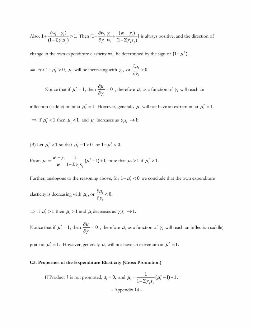
is always positive, and the direction of
change in the own expenditure elasticity will be determined by the sign of (1 ).i
For 1 0,i i will be increasing with ,i or 0.i
i
Notice that if 1i , then 0i
i
, therefore i as a function of i will reach an
inflection (saddle) point at 1.i However, generally i will not have an extremum at 1.i
if 1i then 1,i and i increases as i is 1;
(B) Let 1i so that 1 0i
, or 1 0.i
From 1
( 1) 1,1
i ii i
i j j
w
w s
note that 1i if 1i
.
Further, analogous to the reasoning above, for 1 0i we conclude that the own expenditure
elasticity is decreasing with i , or 0.i
i
if 1i then 1i and i decreases as i is 1.
Notice that if 1i , then 0i
i
, therefore i as a function of i will reach an inflection saddle)
point at 1i . However, generally i will not have an extremum at 1.i
C3. Properties of the Expenditure Elasticity (Cross Promotion)
If Product i is not promoted, 0,is and 1
( 1) 11i i
j js
.
- Appendix 15 -
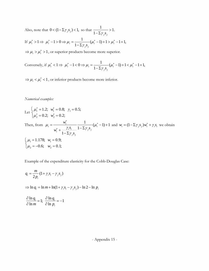
Also, note that 0 (1 ) 1,j js so that 1
1.1 j js
If 1i
11 0 ( 1) 1 1 1,
1i i i ij js
1i i , or superior products become more superior.
Conversely, if 1i
11 0 ( 1) 1 1 1,
1i i i ij js
1i i , or inferior products become more inferior.
Numerical examples:
Let 1 1 1
2 2
1.2; 0.8; 0.5;
0.2; 0.2;
w
w
Then, from 1
( 1) 11
1
ii i
i i j ji
j j
ws sw
s
and (1 )i j j i i iw s w s we obtain
2
1
2
11.178; 0.9;
0.6; 0.1;
w
w
Example of the expenditure elasticity for the Cobb-Douglas Case:
(1 )2i i i j j
i
mq s s
p
ln ln ln(1 ) ln 2 lni i i j j iq m s s p
ln
1;ln
iq
m
ln1
lni
i
q
p
- Appendix 16 -
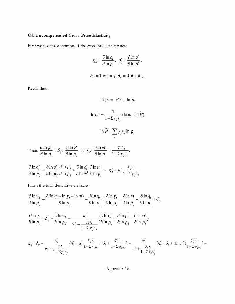
C4. Uncompensated Cross-Price Elasticity
First we use the definition of the cross price-elasticities:
ln,
lni
iji
q
p
ln
,ln
iij
i
q
p
1ij if , 0iji j if i j .
Recall that:
ln ip lni i is p
1ln (ln ln )
1 j j
m m Ps
ln lnj j jj
P s p
Then, ln
;ln
iij
i
p
p
ln;
ln j jj
Ps
p
ln
.ln 1
j j
j j j
sm
p s
lnln ln ln ln
ln ln ln ln lnji i i
j j j j
pq q q m
p p p m p
1j j
ij ij j
s
s
From the total derivative we have:
ln (ln ln ln ) ln ln lnln
ln ln ln ln ln lni i i i i i
ijj j j j j j
w q p m q p qm
p p p p p p
ln ln ln ln ln( ).
ln ln ln ln ln1
i i i i iij
i ij j j j ji
j j
q w w q p msp p p p pw
s
( ) [ (1 ) ]1 1 1
1 1
j j j j j ji iij ij ij i ij ij ij i
i i i ij j j j j ji i
j j j j
s s sw ws ss s sw w
s s
- Appendix 17 -
(1 )[ (1 ) ] [(1 )( ) (1 ) ];
(1 ) 1j j i j j i
ij ij i j j ij ij i j jj j i i i j j i
s w s ws s
s w s s w
[( ) (1 ) ] (1 )( ) (1 )(1 ) .1 1
j j j ji i i i i i iij ij ij ij i ij ij i
i j j i i j j
s sw s s s
w s w w s
We know that ( 1)
1 ,1
(1 )1
ii
i i
i j j
s
w s
(1 )( ) ( 1)i iij ij ij ij i j j
i
ss
w
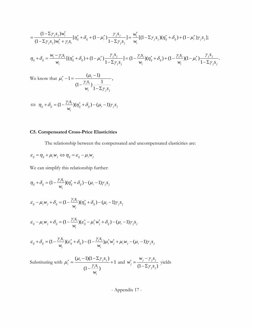
C5. Compensated Cross-Price Elasticities
The relationship between the compensated and uncompensated elasticities are:
ij ij i j ij ij i jw w
We can simplify this relationship further:
(1 )( ) ( 1)i iij ij ij ij i j j
i
ss
w
(1 )( ) ( 1)i iij i j ij ij ij i j j
i
sw s
w
(1 )( ) ( 1)i iij i j ij ij i j ij i j j
i
sw w s
w
(1 )( ) (1 ) ( 1)i i i iij ij ij ij i j i j i j j
i i
s sw w s
w w
Substituting with ( 1)(1 )
1(1 )
i j ji
i i
i
s
s
w
and
(1 )j j j
jj j
w sw
s
yields
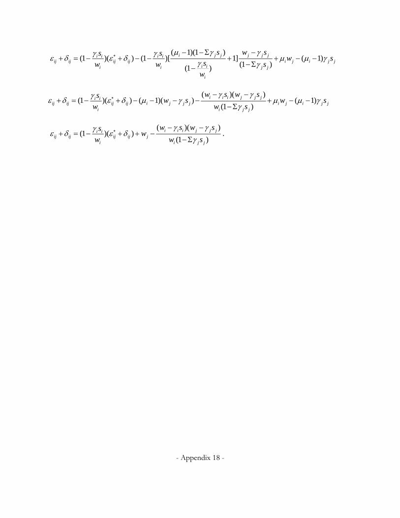
- Appendix 18 -
( 1)(1 )
(1 )( ) (1 )[ 1] ( 1)(1 )(1 )
i j j j j ji i i iij ij ij ij i j i j j
i ii i j j
i
s w ss sw s
sw w sw
( )( )(1 )( ) ( 1)( ) ( 1)
(1 )i i i j j ji i
ij ij ij ij i j j j i j i j ji i j j
w s w ssw s w s
w w s
( )( )
(1 )( )(1 )
i i i j j ji iij ij ij ij j
i i j j
w s w ssw
w w s
.