Embed Size (px)
Citation preview

The Modeling of Surface TNR’s on Compact Stars
• Nova – review
• X-Ray bursts on NS – first steps
Multidimensional NovaSimulations
• Why ?
• Who ?
• How ?
• What’s Now ?
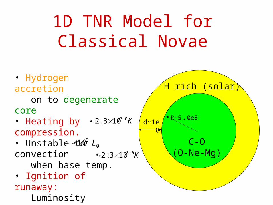
1D TNR Model for Classical Novae
K07103:2
K08103:2
H rich (solar) • Hydrogen accretion on to degenerate core• Heating by compression. • Unstable to convection when base temp. • Ignition of runaway: Luminosity peak temperatures
C-O(O-Ne-Mg)
R~5.0e8d~1e8
0510 L
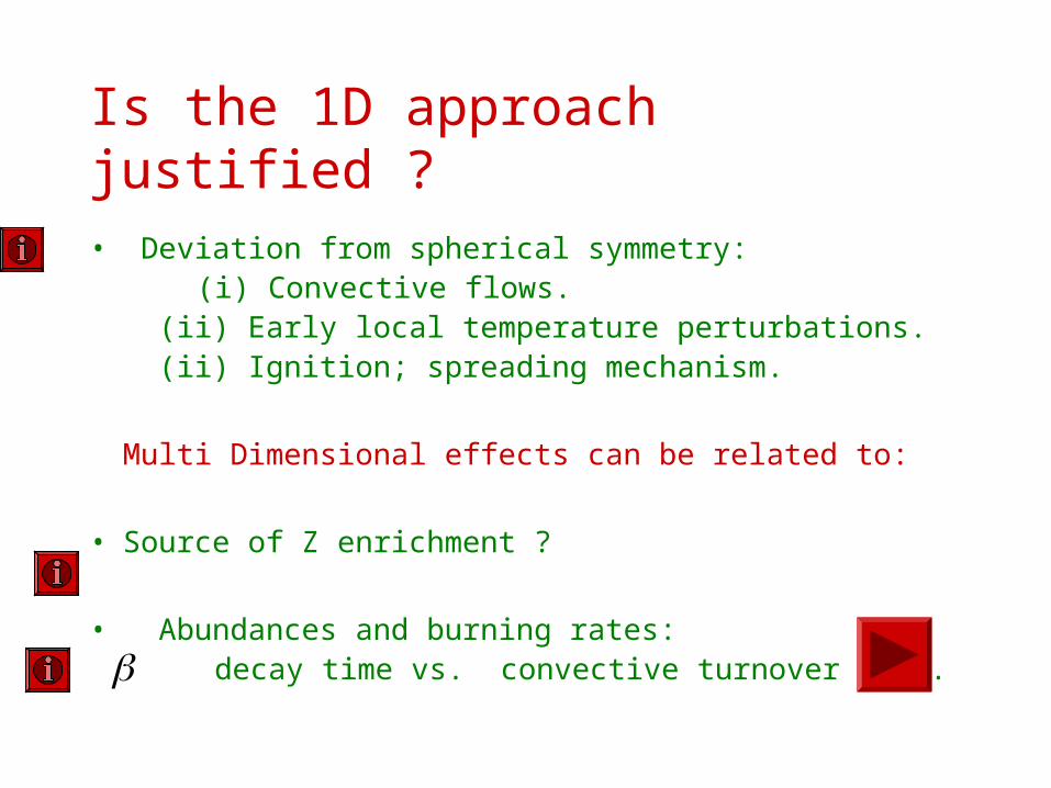
Is the 1D approach justified ?
• Deviation from spherical symmetry: (i) Convective flows. (ii) Early local temperature perturbations. (ii) Ignition; spreading mechanism.
Multi Dimensional effects can be related to:
• Source of Z enrichment ?
• Abundances and burning rates: decay time vs. convective turnover time.

H rich (solar)
C-O(O-Ne-Mg)
R~5.0e8d~1e8
Local perturbation
1D Temperature history

Time Scales• Dynamic ~ 1 sec (sound crossing time)• Thermal diffusion ~ 100-1000 years• Convection (1D MLT) :
V~10^6 cm/sec , scale height~5*10^7 cm
Turnover time~50 sec• Burning:
Depends on temperature and composition
0.1 sec at 10^8 K
10^4 sec at 7*10^7 K
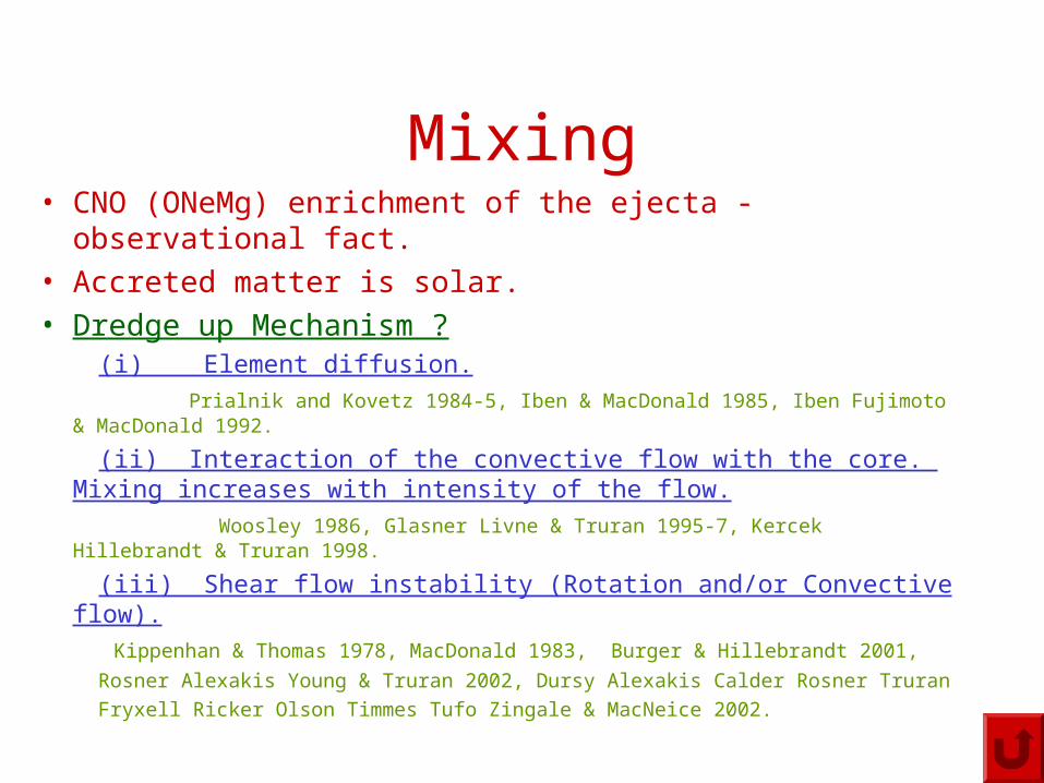
Mixing• CNO (ONeMg) enrichment of the ejecta - observational fact.
• Accreted matter is solar.
• Dredge up Mechanism ? (i) Element diffusion.
Prialnik and Kovetz 1984-5, Iben & MacDonald 1985, Iben Fujimoto & MacDonald 1992.
(ii) Interaction of the convective flow with the core. Mixing increases with intensity of the flow.
Woosley 1986, Glasner Livne & Truran 1995-7, Kercek Hillebrandt & Truran 1998.
(iii) Shear flow instability (Rotation and/or Convective flow).
Kippenhan & Thomas 1978, MacDonald 1983, Burger & Hillebrandt 2001,
Rosner Alexakis Young & Truran 2002, Dursy Alexakis Calder Rosner Truran
Fryxell Ricker Olson Timmes Tufo Zingale & MacNeice 2002.
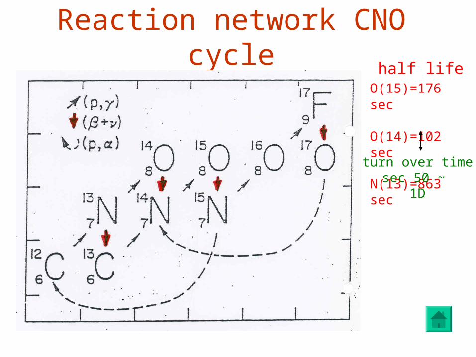
Reaction network CNO cycle
half life O(15)=176 sec O(14)=102 sec N(13)=863 sec
turn over time ~ 50 sec
1D

Who ? How ?Kercek, Hillebrandt & TruranShankar, Arnett & Fryxell
Glasner, Livne & Truran Alexakis, Young, Rosner, Truran, Hillebrandt, and the Flash Code Team
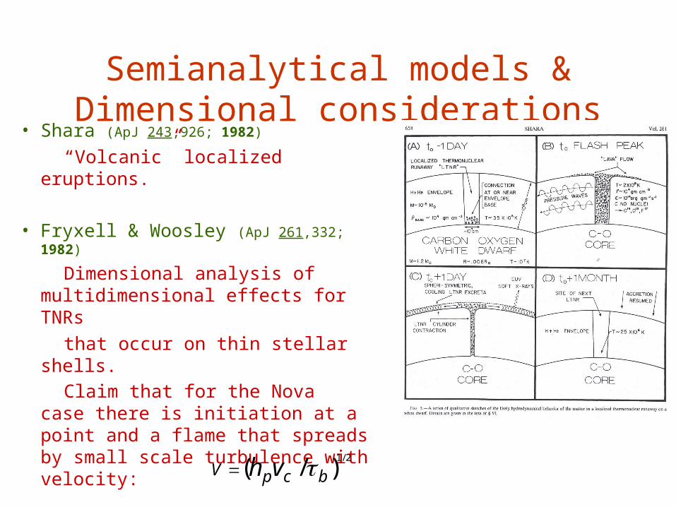
Semianalytical models & Dimensional considerations
• Shara (ApJ 243,926; 1982)
“Volcanic” localized eruptions.
• Fryxell & Woosley (ApJ 261,332; 1982)
Dimensional analysis of multidimensional effects for TNRs
that occur on thin stellar shells.
Claim that for the Nova case there is initiation at a point and a flame that spreads by small scale turbulence with velocity:
)/(2/1
bcpV vh
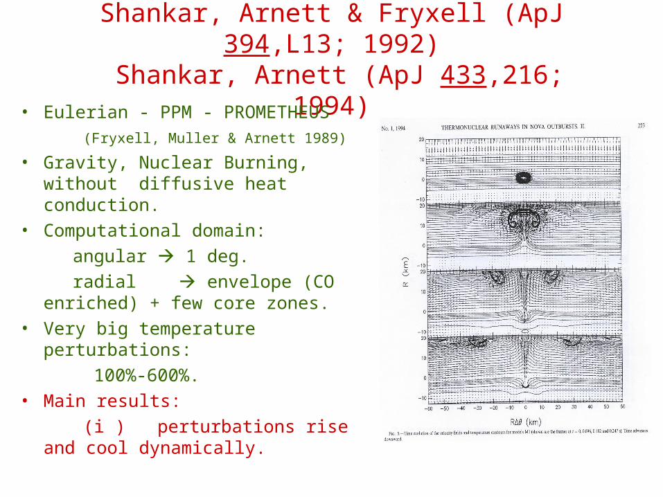
Shankar, Arnett & Fryxell (ApJ 394,L13; 1992) Shankar, Arnett (ApJ 433,216; 1994)
• Eulerian - PPM - PROMETHEUS
(Fryxell, Muller & Arnett 1989)
• Gravity, Nuclear Burning, without diffusive heat conduction.
• Computational domain:
angular 1 deg.
radial envelope (CO enriched) + few core zones.
• Very big temperature perturbations:
100%-600%.
• Main results:
(i ) perturbations rise and cool dynamically.

Glasner & Livne (ApJ,445,L149; 1995)Glasner, Livne & Truran (ApJ,475,754; 1997)
• ALE – VULCAN – Livne 1993 Explicit – Implicit• Computational domain: angular 20 deg radial envelope (solar) + few core
zones. Size ~ 5x5 Km. • Relax the convective flow; no pertur.• Main results: (i) Mixing by dredge up. (ii) TNR takes place with very
irregular local flames. (iii) No trace for flame propagation. (iv) Convective cells and convective
velocities are bigger than those predicted by 1D MLT.

Kercek, Hillebrandt & Truran (A&A 337,379; 1998)• Eulerian - PPM – improved PROMETHEUS (Fryxell, Muller & Arnett 1989)• Computational domain: same as GLT 1997.• Cell Size ~ 5x5 Km. (same as GLT) + HIGHER RESOLUTION ~ 1x1 Km.• Remap the 1D zones, Relax hydro, Ignition in one zone.
• Main results: (i) Direct numerical 2D simulations of
TNRs are feasible. (ii) Signs for convergence for higher
resolution. (iii) General outcome resembles GLT 1997 (iv) Mixing by dredge up but at a later stage. (iv) Somewhat less violent.
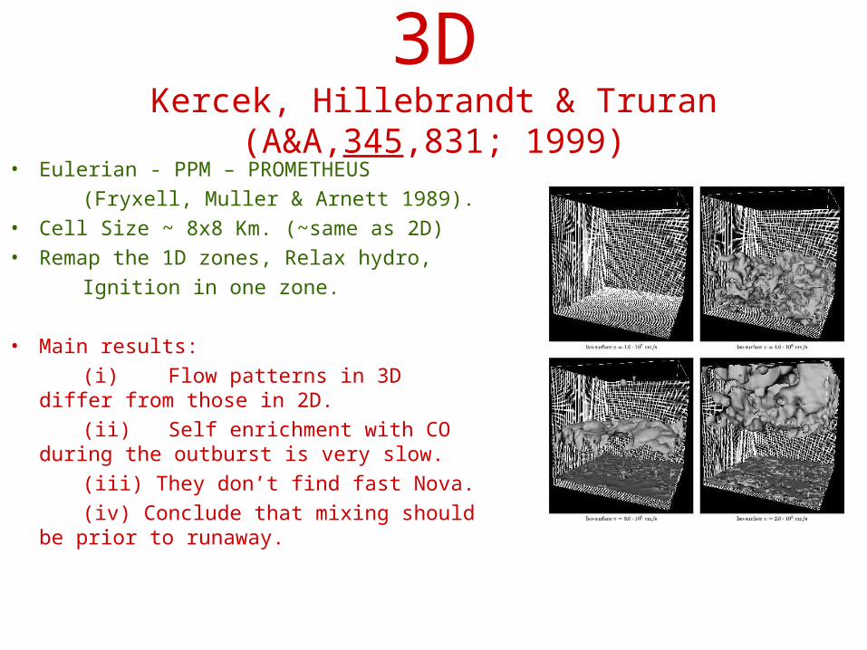
3DKercek, Hillebrandt & Truran (A&A,345,831; 1999)
• Eulerian - PPM – PROMETHEUS
(Fryxell, Muller & Arnett 1989).
• Cell Size ~ 8x8 Km. (~same as 2D)
• Remap the 1D zones, Relax hydro,
Ignition in one zone.
• Main results:
(i) Flow patterns in 3D differ from those in 2D.
(ii) Self enrichment with CO during the outburst is very slow.
(iii) They don’t find fast Nova.
(iv) Conclude that mixing should be prior to runaway.

A few of the things we learned up to now

Ignition process
• TNR takes place with very irregular local flames no trace for flame propagation.
• We can follow the ignition process almost
from the set on of convection.
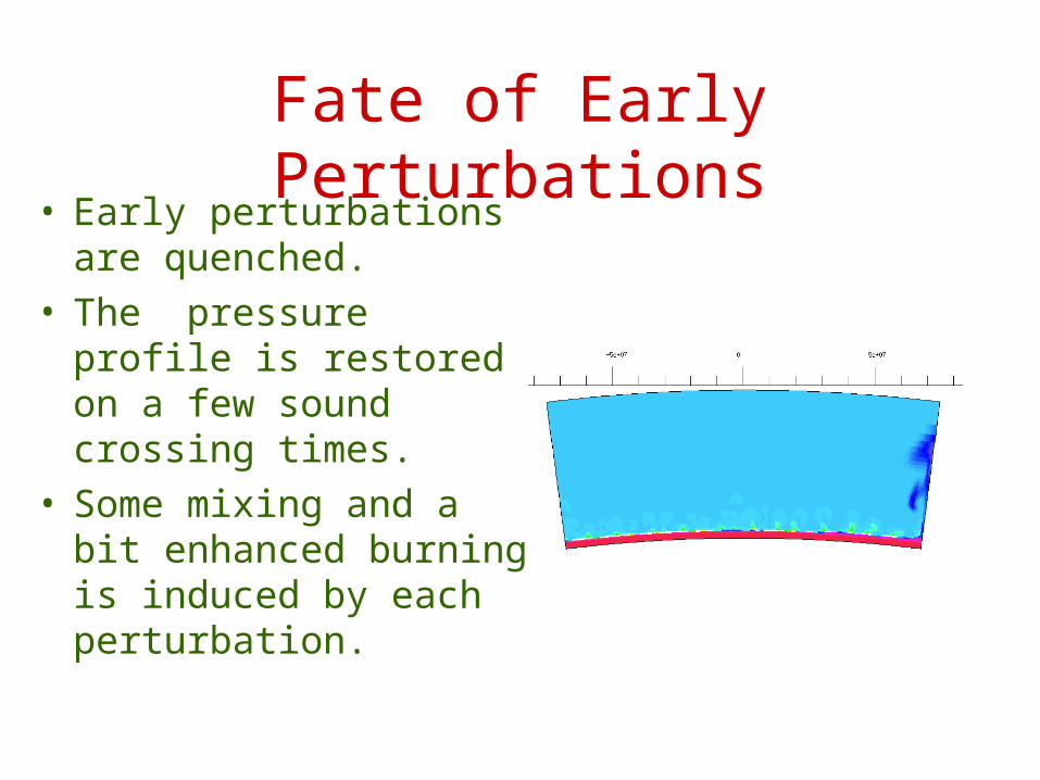
Fate of Early Perturbations• Early perturbations are
quenched. • The pressure profile is
restored on a few sound crossing times.
• Some mixing and a bit enhanced burning is induced by each perturbation.
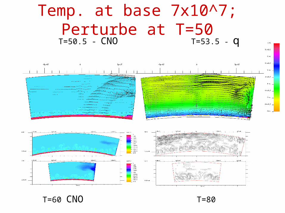
Temp. at base 7x10^7; Perturbe at T=50T=50.5 - CNO T=53.5 - q
T=60 CNO T=80

Burning rates – time history

Mixing• Macroscopic overshot
(undershoot) mixing exists from the moment the flow becomes unstable to convection. The amount of mixing increases
(not linearly) with the approach towards runaway conditions.
Eulerian=>advection=>
Numerical Mixing !!!

• Without mixing burning rates are limited by proton capture on C12:
Dredge up of fresh C12 on times shorter than beta decay time can lead to extreme burning rates that are temperature dependent
Burning rates
)01.0/(108.5 13max cnoZq

What are the differences ?
• Can we explain fast Nova ?
• What is the amount of mixing during each stage of the runaway ?
• What is the topology of the convective cells ?

Why is it hard ?&
What are the reasons for the differences ?
• Mapping the 1D initial model to 2D.
• Discontinuities in the initial model.
• Sensitivity of the burning rates to the exact amount of mixing.
• Sensitivity to the outer boundary conditions.
• The role of hydrodynamic instabilities (KH).

Tmp
Initial Model
rho
P
CNO
Steep gradients at the base of the envelope

Dependence of Q on the amount of mixing
of cold C12 with hot Hydrogen

Demonstration of the sensitivity to the outer boundary conditions
Time=130 Time=400

and indeed…

The future is…
INSTABILITIES !!!
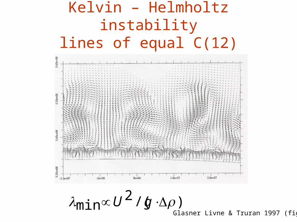
Kelvin – Helmholtz instabilitylines of equal C(12) abundance
Glasner Livne & Truran 1997 (fig.2))/(2
min gU

What should be done ?&
Who started to do homework ?

Theoretical analysis and simulations of
Mixing through shear instabilities
• Distinct between: (i) KH Instability due to a velocity jump. (ii) Critical Layer Instability - Shear flow drive gravity waves by resonant interaction when both have the
same velocity –> Non linear “breaking waves” induce mixing.• Linear analysis of the instabilities in order to find the relevant
control parameters and the relevant unstable modes.• Use the acquired knowledge in order to perform ‘wise’
simulations putting efforts to resolve the relevant modes. • Work in those directions is done by the Flash code team in
Chicago and at the Max Planck Institute.

Induced mixing by shear wind
The Flash code team ; Chicago

NOVA Temp=4e7 t=10

T=20 v_scale=2e7

T=38

T=38
Flashes on NS
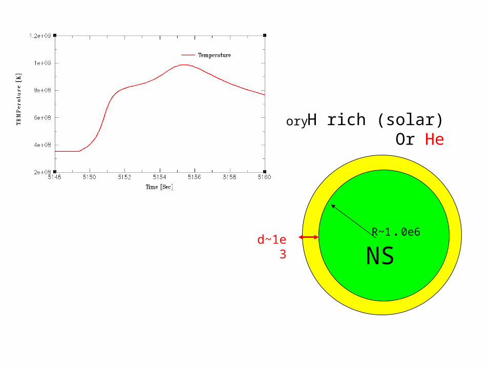
H rich (solar)Or He
NSR~1.0e6
d~1e3
1D Temperature history

Time Scales• Dynamic ~ 1 micro sec (sound crossing
time)
• Thermal diffusion ~ 10-100 Sec
• Convection (1D MLT) :
V~10^6 cm/sec , scale height~ 10-100 cm
Turnover time~10^(-5) sec
• Burning: The whole fuel is consumed
• Rotation ~ 10^(-3) Sec.
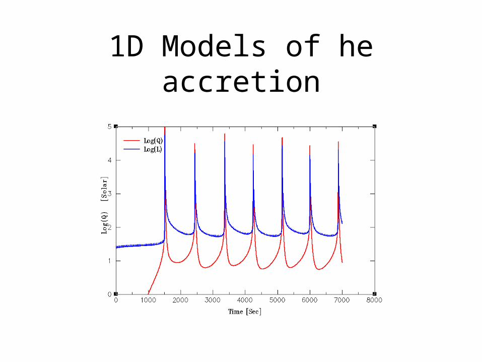
1D Models of he accretion

Fryxell & Woosley 1982 ApJThey give three different
phenomenological estimates for the speed of the front:
• The width of the front is equal to the length scale of a convective cell, taken to be the scalehight.
v=(h_scale/t_nuc) ~ 10^4 cm/sec
• Heat is transported by turbulent convective diffusion.
v=Sqrt(D/t_nuc) ~ 2*10^5 cm/sec D=h_scale*v_conv
• The turbulent scale is much larger than the front width
v=v_conv ~ a few 10^6 cm/sec


Global energy production ratefor 2D modelWithout any perturbation Temp=6e8
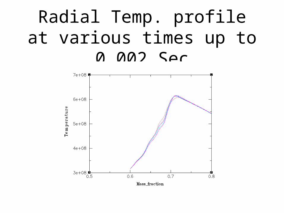
Radial Temp. profile at various times up to 0.002 Sec

Perturbation Temp 6e8=>2e9At Time=0
Non existing initial velocity field

T=3e-7
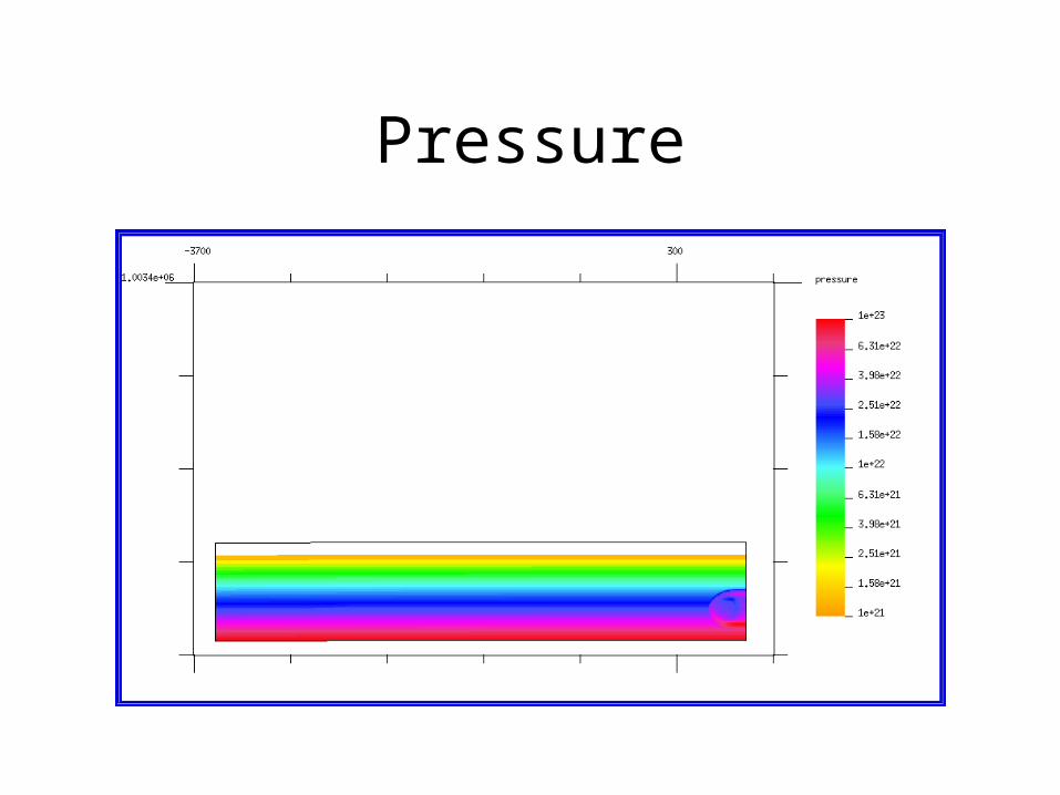
Pressure

T=1e-6

Pressure 1.0e-6

T=2e-6

Pressure

T=5e-6

Pressure t=5e-6

T=6e-6

T=7e-6
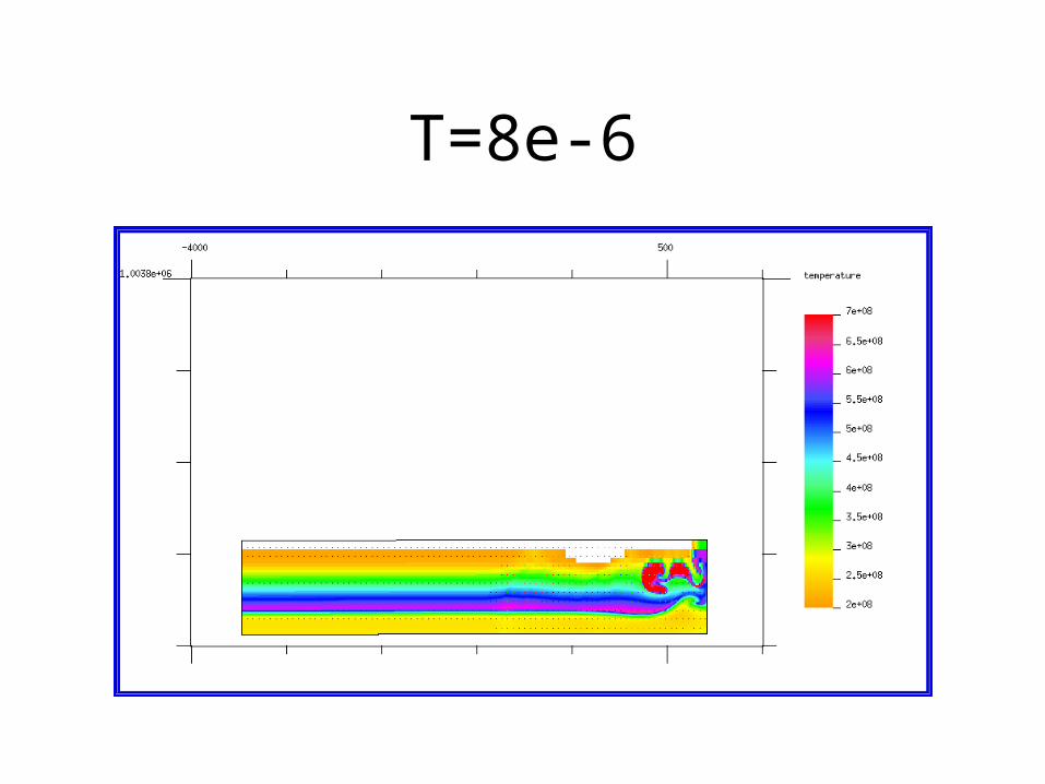
T=8e-6

T=9e-6

T=10e-6

Pressure t=10e-6

T=11e-6

T=16e-6

Perturbation Temp 6e8=>2e9At Time=2.7e-3 sec
existing initial convective velocity field

Temp=2e9 t0=2.701e-3

V_scale=2e8

Pressure
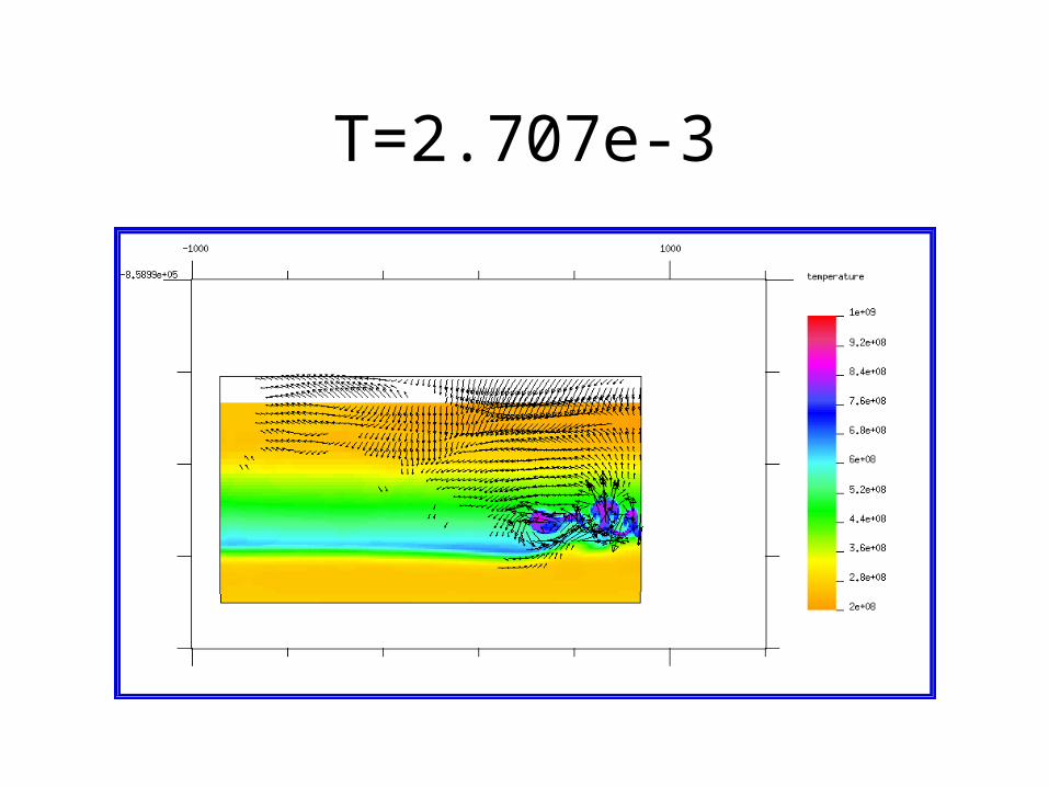
T=2.707e-3
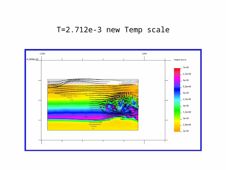
T=2.712e-3 new Temp scale
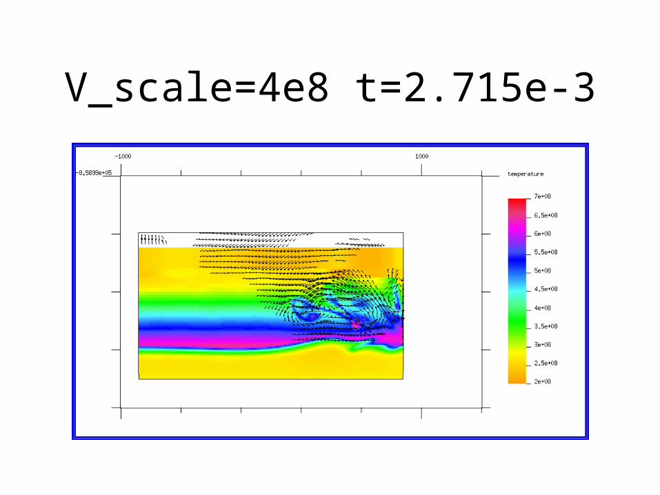
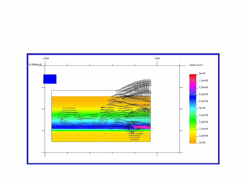
V_scale=4e8 t=2.715e-3
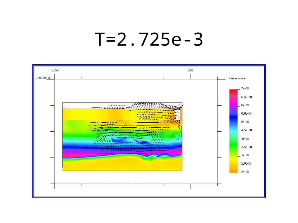
T=2.725e-3

Perturbation Temp 6e8=>8e8At Time=2.7e-3 sec
existing initial convective velocity field

Convective Temp_pertube=8e8t=2.701e-3 dt=1.0e-6 v_scale=5e7

Press t=2.701e-3
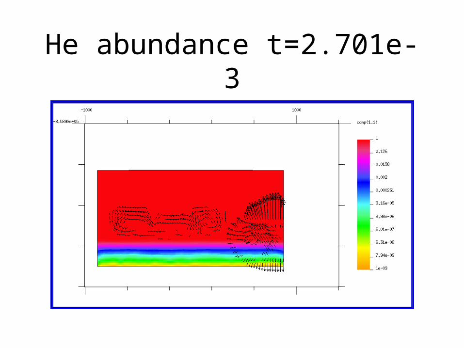
He abundance t=2.701e-3


2.704e-3

T=2.707e-3

T=2.709 v_scale=1e8

T=2.713e-3 v-scale=2e8
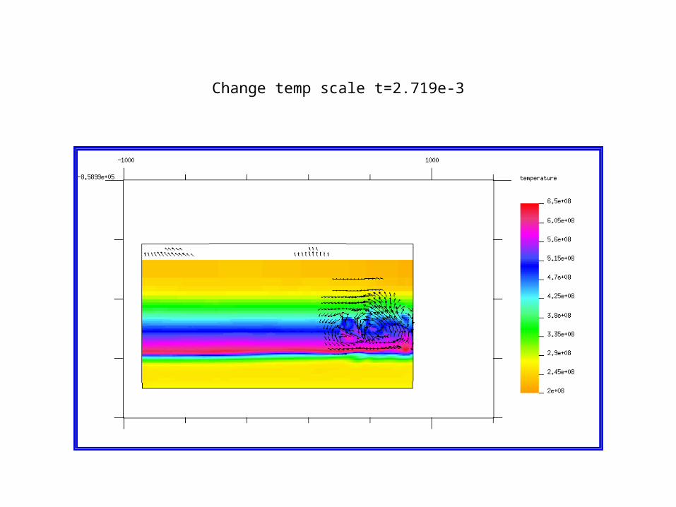
Change temp scale t=2.719e-3

T=2.735e-3
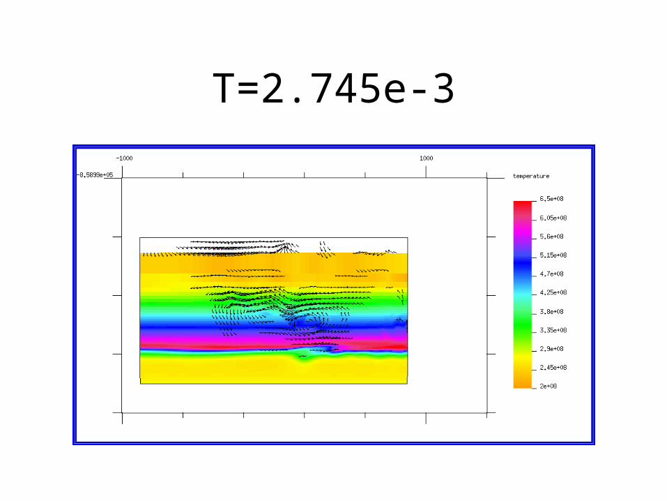
T=2.745e-3

T=2.755e-3

END