Principles for Optimal Control, Part 2!

Robert Stengel! Optimal Control and Estimation, MAE 546, Princeton

University, 2017

•! Minimum Principle•! Hamilton-Jacobi-Bellman Equation

(Dynamic Programming)•! Terminal State Equality Constraint•! Linear, Time-Invariant, Minimum-Time

Control Problem

Copyright 2017 by Robert Stengel. All rights reserved. For educational use only.http://www.princeton.edu/~stengel/MAE546.html

http://www.princeton.edu/~stengel/OptConEst.html 1

The Minimum Principle!

2

The Minimum Principle*

!H[x(t),u(t),""(t),t]!u

= 0 in t0 ,t f( )

! 2H[x(t),u(t),""(t),t]!u2 > 0 in t0 ,t f( )

H*= H x*(t),u*(t),!! "" (t)[ ]# H x*(t),u(t),!! "" (t)[ ]

Variational necessary and sufficient conditions imply that minimum H is optimal

* After the Maximum Principle of Pontryagin, et al, 1950s (opposite convention for sign of Hamiltonian)

3

Control Perturbation Can Only Increase Cost

J u*(t)+ !u(t)[ ]" J u*(t)[ ] = # x*(t f )$% &' "# x*(t f )$% &'

+ H x*(t),u*(t)+ !u(t),(( )) (t)[ ]" (( ))T (t)!x*(t){ }" H x*(t),u*(t),(( )) (t)[ ]" (( ))T (t)!x*(t){ }t0

t f

* dt

J u*(t)+ !u(t)[ ]" J u*(t)[ ] =

H x*(t),u*(t)+ !u(t),## $$ (t)[ ]{ }" H x*(t),u*(t),## $$ (t)[ ]{ }t0

t f

% dt & 0

Effect of control perturbation on optimal H and J *

Control perturbation has no effect on terminal cost or !!T "x"t

Assuming that x* t( ) and !! * t( ) are the optimal values 4

Optimal x(t)

Application of the Minimum Principle with Bounded Control

•! Minimum principle applies –! when control is limited such

that !H/!u " 0–! in some cases of singular

control, e.g. bang-bang control (TBD)

5

Dynamic Programming!

6

Cost Function vs. Value Function

J * t1( ) = L x(! ),u(! )[ ]t0

t1

" d!

Optimal Cost Function (i.e., accrued cost) at t1

J * t f( ) = ! x(t f )"# $% + L x(& ),u(& )[ ]

t0

t f

' d& ! J *max

Optimal Cost Function at tf

Cost

7

Cost Function vs. Value Function

Optimal Value Function (i.e., remaining cost) at t1

V * x1,t1( ) = ! x * (t f )"# $% + L x * (& ),u * (& )[ ]t1

t f

' d&

= ! x * (t f )"# $% ( L x * (& ),u * (& )[ ]t f

t1

' d&

= minu

! x * (t f )"# $% ( L x * (& ),u(& )[ ]t f

t1

' d&)*+

,+

-.+

/+

Optimal Value Function at to

V * xo,to( ) = ! x*(t f )"# $% & L x*(' ),u*(' )[ ]t f

t0

( d'

!V *max ) J *max

Value = Cost-to-Go

8

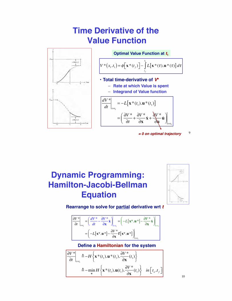
Time Derivative of the Value Function

V * x1,t1( ) = ! x * (t f )"# $% & L x * (' ),u * (' )[ ]t f

t1

( d'

•!Total time-derivative of V*–! Rate at which Value is spent–! Integrand of Value function

dV *dt t=t1

= !L x*(t1),u*(t1)[ ]

= "V *"t

+ "V *"x!x + "V *

"u!u#

$%&'(t=t1

= 0 on optimal trajectory

Optimal Value Function at t1

9

Dynamic Programming: !Hamilton-Jacobi-Bellman

EquationRearrange to solve for partial derivative wrt t

!V *!t t=t1

= dV *dt

" !V *!x!x#

$%&'(t=t1

= "L x*,u*[ ]" !V *!x!x#

$%&'(t=t1

= "L x*,u*[ ]" !V *!x

f x*,u*[ ]#$%

&'(t=t1

!V *!t t=t1

! "H x*(t1),u*(t1),!V *!x

(t1)#$%

&'(

! "minuH x*(t1),u(t1),

!V *!x

(t1)#$%

&'(

in to,t f)* +,

Define a Hamiltonian for the system

10

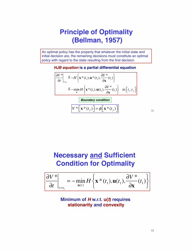
Principle of Optimality (Bellman, 1957)

An optimal policy has the property that whatever the initial state and initial decision are, the remaining decisions must constitute an optimal policy with regard to the state resulting from the first decision.

!V *!t t=t1

! "H x*(t1),u*(t1),!V *!x

(t1)#$%

&'(

! "minuH x*(t1),u(t1),

!V *!x

(t1)#$%

&'(

in to,t f)* +,

HJB equation is a partial differential equation

Boundary condition

V * x * (t f )!" #$ = % x * (t f )!" #$ 11

Necessary and Sufficient Condition for Optimality

!V *!t t= t1

= "minu(t )

H x * (t1),u(t1),!V *!x

(t1)#$%

&'(

Minimum of H w.r.t. u(t) requires stationarity and convexity

12

V*[x(t),t] is a Hypersurface That Defines Minimum Cost Control

•!V*[x(t),t] is the integral of the HJB equation–! V* is a scalar function of the state

•! Ideally, the time-varying hypersurface of V* is bowl-shaped

•!Minimum of hypersurface specifies optimal control policy

Time

u * t( ) = u * V * x * t( )!" #${ }

V * x * (t f )!" #$ = % x * (t f )!" #$

At the terminal time

13

Relationship of HJB Equation to Other Principles of Optimality

Calculus of Variations (Euler-Lagrange Equations)

!V *!x

(t1) = ""T (t1)

minuH x*(t1),u(t1),

!V *!x

(t1)"#$

%&'in t0,t f() *+ defines optimality

Minimum Principle

!V *!t t=t1

! "H x*(t1),u*(t1),!V *!x

(t1)#$%

&'(

! "minuH x*(t1),u(t1),

!V *!x

(t1)#$%

&'(in t0,t f)* +,

14

Space Shuttle Reentry Example!

15

Optimal Guidance for Space Shuttle Reentry

DGO = Distance to GoAGO = Azimuth to Go

16

Optimal Trajectories for !Space Shuttle Reentry

Altitude vs. Velocity Range vs. Cross-Range ( footprint )

Numerical solutions using steepest-descent and conjugate-gradient algorithms17

Optimal Controls for

Space Shuttle Reentry

Angle of Attack vs. Specific Energy

!! Independent variable is specific total energy rather than time

!! On reentry, total energy decreases as time increases

Roll Angle vs. Specific Energy

18

Optimal Guidance System Derived from Optimal Trajectories

Angle of Attack and Roll Angle vs. Specific Energy

Diagram of Energy-Guidance Law

19

Guidance Functions for !Space Shuttle Reentry

Angle of Attack Guidance Function

Roll Angle Guidance Function

•!Guidance surfaces can be implemented with–! Table lookup–! Computational neural networks

20

Terminal State Equality Constraint!

21

Minimize a Cost Function Subject to a Terminal State Equality Constraint

minu(t )

J = ! x(t f )"# $% + L x(t),u(t)[ ]ti

t f

& dt

!x(t) = f[x(t),u(t)], x to( ) given

! x(t f )"# $% & 0 (scalar)

Dynamic Constraint

Terminal State Equality Constraint

!! subject to

22

Terminal State Equality ConstraintsSoft Constraint (= terminal cost)

Hard Constraint

! x(t f )"# $% & 0

minu(t )

! x(t f )"# $%, e.g., ! x(t f )"# $% = kxT t f( )x t f( )

! x(t f )"# $% ! 0 is OK

! x(t f )"# $% = x1 f & xD ' 0

! x(t f )"# $% = x1 f & xD ' 0

Examples

23

Cost Function Augmented by Terminal State Equality Constraint

JConstrained = JUnconstrained + µ! x(t f )"# $%! J0 + µJ1

µ = constant scalar Lagrange multiplier for terminal constraint

!! Separate solution into two parts!! Optimize original cost function alone!! Optimize for constraint alone

24

Euler-Lagrange Equations and 1st Variation for Unconstrained

Optimization!!0 (t f ) =

"#[x(t f )]"x

$%&

'()

T

!!!0 = " #H0[x,u,!!0,t]

#x$%&

'()

T

= " #L#x

+ !!0T # f#x

*+,

-./

T

= " Lx + FT!!0*+ -.

!J0 ="H0

"u!u#

$%&'(

ti

t f

) dt = Lu + **0TG( )!u

ti

t f

) dt

Assuming that these equations are satisfied, the first variation is

25

Terminal Constraint Cost Augmented by Dynamic Constraint

J1 =! x(t f )"# $% + &&1T (t) f[x(t),u(t)]' !x(t)[ ]{ }

ti

t f

( dt

=! x(t f )"# $% + &&1T f[x,u]' &&1

T !x{ }ti

t f

( dt

J1 !! x(t f )"# $% + H1[x,u,&&1T ]' &&1

T "x{ }ti

t f

( dt

=! x(t f )"# $% + &&1T (t0 )x(t0 )' &&1

T (t f )x(t f )"# $%

+ H1 x,u,&&1[ ]+ "&&1Tx{ }ti

t f

( dt H1 ! !!1T f[x,u]

26

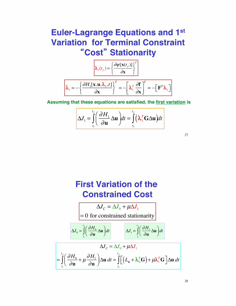
Euler-Lagrange Equations and 1st Variation for Terminal Constraint

Cost Stationarity!!1(t f ) =

"# [x(t f )]"x

$%&

'()

T

!!!1 = "

#H1[x,u,!!1,t]#x

$%&

'()

T

= " !!1T #f#x

*+,

-./

T

= " FT!!1*+ -.

!J1 ="H1

"u!u#

$%&'(

ti

t f

) dt = **1TG!u( )

ti

t f

) dt

Assuming that these equations are satisfied, the first variation is

27

First Variation of the Constrained Cost

!J1 ="H1

"u!u#

$%&'( dt

ti

t f

)

!JC = !J0 + µ!J1

= 0 for constrained stationarity

!J0 ="H0

"u!u#

$%&'( dt

ti

t f

)

!JC = !J0 + µ!J1

= "H0

"u+ µ "H1

"u#$%

&'( !u

ti

t f

) dt = Lu + **0TG( ) + µ**1

TG+, -.!uti

t f

) dt

28

First Variation of the Constrained Cost

!JC = !J0 + µ!J1 = 0

= "H0

"u+ µ "H1

"u#$%

&'( !u

ti

t f

) dt = Lu + **0TG( ) + µ**1

TG+, -.!uti

t f

) dt

Control perturbation is arbitrary, so chose

!u = " #H1

#u$%&

'()T

= " **1TG( )T , " = arbitrary constant

29

First Variation of the Constrained Cost

!JC = Lu + ""0TG( ) + µ""1

TG#$ %&'GT""1

ti

t f

( dt

= ' Lu + ""0TG( )GT""1 + µ""1

TGGT""1#$ %&ti

t f

( dt

= ' Lu + ""0TG( )GT""1#$ %&

ti

t f

( dt + µ ""1TGGT""1#$ %&

ti

t f

( dt)*+

,+

-.+

/+! ' a + µb( )

!JC = 0 if µ = " ab

Solution for terminal constraint Lagrange multiplier

30

Controllability Gramian

b ! !!1

T t( )G t( )GT t( )!!1 t( )"# $%ti

t f

& dt ' 0

For control of the terminal constraint, the controllability gramian must not equal zero

A sufficient condition for optimality

31

Optimizing Control for Terminal Constraint

!HC

!u= !H0

!u" a

b#$%

&'(!H1

!u)*+

,-.

= Lu + //0TG( )" a

b#$%

&'( //1

TG)*+

,-.= 0

Choose u t( ) such that

32

Linear, Time-Invariant Minimum-Time Problem!

33

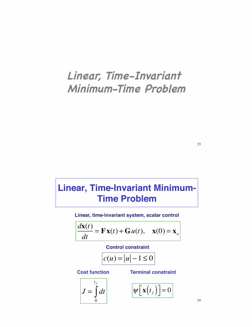
Linear, Time-Invariant Minimum-Time Problem

dx(t)dt

= Fx(t) +Gu(t), x(0) = xo

Linear, time-invariant system, scalar control

Control constraint

c(u) = u !1 " 0

Cost function

J = dt0

t f

!

Terminal constraint

! x t f( )"# $% = 034

Linear, Time-Invariant Minimum-Time Problem

HC = 1+ !!T Fx +Gu( ) + µ"Hamiltonian

Adjoint equation

!!! = "

#HC

#x$%&

'()T

= "FT!!, !! t f( ) = #*#x

t f( )+,-

./0

Open-end time problem

HC * t f( ) = 0Time-invariant problem

HC * t( ) = 0 on entire trajectory35

Linear, Time-Invariant Minimum-Time Problem

!HC

!u= ""TG , #

!2HC

!u2 = 0 $ Singular problem (not convex)

Standard optimality conditions not satisfied

Minimum principle (smallest Hamiltonian) solves the problem1+ !! ""T Fx *+Gu *( ) #1+ !! ""T Fx *+Gu( )

!! ""T Gu *( ) # !! ""T Gu( )!! ""T G( )u*# !! ""T G( )u, most negative value

Optimal control is a switching law u* =

+1, !! ""T G < 0

#1, !! ""T G > 0

$%&

'& 36

Bang-Bang Control of the Lunar Module

!!(t)!q(t)

"

#$$

%

&''= 0 1

0 0"

#$

%

&'

!(t)q(t)

"

#$$

%

&''+

0gA / Iyy

"

#$$

%

&''u(t)

Time evolution of the state while a thruster is on [u(t) = 1]Angular rate, deg/s: q(t) = gA / Iyy( )t + q(0)

Angle, deg: !(t) = gA / Iyy( )t 2 / 2 + q(0)t +!(0)

Neglecting initial conditions, what does the phase-plane plot (pitch rate vs. pitch angle) look like?

Second-order system with ON/OFF reaction control

37

Constant-Thrust (Acceleration) Trajectories

For u = 1,Acceleration = gA/Iyy

Thrusting away from the origin

Thrusting to the origin

With zero thrust, what does the phase-plane plot look like?

For u = –1,Acceleration = –gA/Iyy

38

Switching-Curve Control Law for On-Off Thrusters

•! Origin (i.e., zero rate and attitude error) can be reached from any point in the state space

•! Control logic:–! Thrust in one

direction until switching curve is reached

–! Then reverse thrust

–! Switch thrust off when errors are zero

39

Next Time:!Constraints and

Numerical Optimization!!

Reading!OCE: Section 3.5, 3.6!

40

SSuupppplleemmeennttaarryy MMaatteerriiaall

41

Apollo Lunar Module Control•! 16 reaction control thrusters

–! Control about 3 axes–! Redundancy of thrusters

•! LM Digital Autopilot

42

Apollo Lunar Module Phase-Plane Control Logic

•! Coast zones conserve RCS propellant by limiting angular rate•! With no coast zone, thrusters would chatter on and off at

origin, wasting propellant•! State limit cycles about target attitude•! Switching curve shapes modified to provide robustness

against modeling errors–! RCS thrust level–! Moment of inertia 43

Apollo Lunar Module Phase-Plane Control Law

•! Switching logic implemented in the Apollo Guidance & Control Computer

•! More efficient than a linear control law for on-off actuators

44

Typical Phase-Plane Trajectory

•! With angle error, RCS turned on until reaching OFF switching curve

•! Phase point drifts until reaching ON switching curve•! RCS turned off when rate is 0-•! Limit cycle maintained with minimum-impulse RCS firings

–! Amplitude = ±1 deg (coarse), ±0.1 deg (fine)

45