The Min-Max Multi-Depot Vehicle Routing Problem:Three-Stage Heuristic and Computational Results

X. Wang, B. Golden, and E. WasilPOMS -May 4, 2013

Overview

•Introduction

•Literature review

•Heuristic for solving the Min-Max MDVRP

•Computational results

•Conclusions

1

3

Introduction• The Min-Max Multi-Depot Vehicle Routing

Problem

4

Introduction

• In the Multi-Depot VRP, the objective is to minimize the total distance traveled by all vehicles

• In the Min-Max MDVRP, the objective is to minimize the maximum distance traveled by the vehicles

5

Introduction•The min-max objective function

6

IntroductionWhy is the min-max objective important?

•Applications ▫Disaster relief efforts

Serve all victims as soon as possible

▫Computer networks Minimize maximum latency between a server and a

client

▫Workload balance Balance amount of work among drivers or across time

horizon

7

Literature Review

•Carlsson et al. (2007) proposed an LP-based balancing approach to solve the Min-Max MDVRP▫Assignment of customers to vehicles by LP▫TSP solved by Concorde▫These steps are repeated and the best feasible

solution is returned

8

Solving the Min-Max MDVRP

•We develop a heuristic (denoted by MD)

•MD has three phases1. Initialization2. Local search3. Perturbation

9

Phase 1: Initialization• Assign customers evenly to vehicles

• Solve a TSP on each route using the Lin-Kernighan heuristic

jix

jm

nor

m

nx

ixts

xc

ij

iij

jij

jiijij

,1,0

1

1..

min,

10

Phase 2: Local Search

•Step 1. From the maximal route, identify the customer to remove (savings estimation)

Customer to remove Savings estimation

11

Phase 2: Local Search

•Step 2. Identify the route to insert the removed customer (cost estimation)

•Step 3. Try inserting the customer in the cheapest way▫Successful – go back to Step 1▫Unsuccessful – try moving another customer

•Step 4. Stop if we have tried to move every customer on the maximal route

12

Phase 3: Perturbation

•Perturb the locations of the depots

13

Phase 3: Perturbation

•Solve the new problem

•Set the depots back the their original positions

•Solve the problem and update the solution

•Repeat the process

14

Computational Results

• 20 test problems▫10 – 500 customers▫3 – 20 depots▫Problems have uniform and non-uniform

customer locations

• MD used an Intel Pentium CPU with 2.20 GHz processor

• Code for LB required a 32-bit machine (Intel Core i5 with 2.40 GHz processor)

15

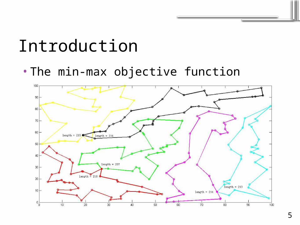
Computational ResultsProblem MM8 (3 depots, 200 customers, 2 vehicles)

16

Computational ResultsProblem MM8 (3 depots, 200 customers, 2 vehicles)

17

Computational ResultsUniform Customer Locations• MD outperforms the LB-based heuristic by 10.7% on average

Identifier

LB MD

Improvement (%)Objective Time (s) Objective Time (s)

MM2 149.225 38.2 131.431 2.80 11.92

MM3 265.349 61.4 236.174 8.20 10.99

MM7 222.071 14.5 189.016 0.74 14.88

MM8 242.730 73.2 215.269 12.56 11.31

MM10 197.594 32.9 197.869 1.33 -0.14

MM11 119.658 78.5 111.067 0.65 7.18

MM12 114.826 37.9 81.300 0.86 29.20

MM13 138.823 35.8 125.268 2.55 9.76

MM14 146.492 35.5 134.476 3.67 8.20

MM15 110.963 41.0 100.074 1.80 9.81

MM16 115.744 60.2 104.125 3.92 10.04

MM18 439.606 68.4 415.777 91.00 5.42

18

Computational ResultsNon-uniform Customer Locations• MD outperforms the LB-based heuristic by 16.2% on average

Identifier

LB MD

Improvement (%)Objective Time (s) Objective Time (s)

MM4 569.453 43.9 488.254 57.7 14.26

MM5 398.970 40.2 330.195 7.7 17.24

MM9 183.157 36.8 153.286 38.1 16.31

MM17 325.708 56.8 253.765 84.4 22.09

MM19 474.935 68.4 395.606 155.8 16.70

MM20 385.297 92.1 344.309 74.2 10.64

19

Computational Results

•On all 20 problems, the running time for MD (596s) is much less than LB (943s)

•Times for MD are between 0.65s and 156s with most times under 13s

•Times for LB are between 6s and 92s

20

Computational Results

Contribution from improvement procedures

21

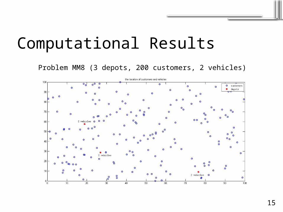
Conclusions

•On the 20 test problems, MD outperforms the LB-based heuristic by 11.27% on average

•In future work, we hope to apply MD to solve a real-world problem

•We want to extend our heuristic to solve min-max problems with service times