Embed Size (px)
Citation preview
The Mid-Latitude Ionosphere: Modeling and Analysis of PlasmaWave Irregularities and the Potential Impact on GPS Signals
Ahmed Said Hassan Ahmed Eltrass
Dissertation submitted to the faculty of theVirginia Polytechnic Institute and State University
in partial fulfillment of the requirements for the degree of
Doctor of Philosophyin
Electrical Engineering
Wayne A. Scales, ChairJ. Michael Ruohoniemi
Sedki M. RiadKathleen MeehanLeigh Winfrey
Hassan M. Elkamchouchi
March 16, 2015Blacksburg, Virginia
Keywords: Ionospheric Irregularities, Plasma Instability, GPS, SuperDARN Radar,Computational Modeling
Copyright 2015, Ahmed Said Hassan Ahmed Eltrass
The Mid-Latitude Ionosphere: Modeling and Analysis of Plasma WaveIrregularities and the Potential Impact on GPS Signals
Ahmed Said Hassan Ahmed Eltrass
ABSTRACT
The mid-latitude ionosphere is more complicated than previously thought, as it includesmany different scales of wave-like structures. Recent studies reveal that the mid-latitudeionospheric irregularities are less understood due to lack of models and observations that canexplain the characteristics of the observed wave structures. Since temperature and densitygradients are a persistent feature in the mid-latitude ionosphere near the plasmapause, thedrift mode growth rate at short wavelengths may explain the mid-latitude decameter-scaleionospheric irregularities observed by the Super Dual Auroral Radar Network (SuperDARN).In the context of this dissertation, we focus on investigating the plasma waves responsible forthe mid-latitude ionospheric irregularities and studying their influence on Global PositioningSystem (GPS) scintillations.
First, the physical mechanism of the Temperature Gradient Instability (TGI), which isa strong candidate for producing mid-latitude irregularities, is proposed. The electro-static dispersion relation for TGI is extended into the kinetic regime appropriate for High-Frequency (HF) radars by including Landau damping, finite gyro-radius effects, and tem-perature anisotropy. The kinetic dispersion relation of the Gradient Drift Instability (GDI)including finite ion gyro-radius effects is also solved to consider decameter-scale waves gen-eration. The TGI and GDI calculations are obtained over a broad set of parameter regimesto underscore limitations in fluid theory for short wavelengths and to provide perspective onthe experimental observations.
Joint measurements by the Millstone Hill Incoherent Scatter Radar (ISR) and the Su-perDARN HF radar located at Wallops Island, Virginia have identified the presence ofdecameter-scale electron density irregularities that have been proposed to be responsible forlow-velocity Sub-Auroral Ionospheric Scatter (SAIS) observed by SuperDARN radars. Inorder to investigate the mechanism responsible for the growth of these irregularities, a timeseries for the growth rate of both TGI and GDI is developed. The time series is computedfor both perpendicular and meridional density and temperature gradients. The growth ratecomparison shows that the TGI is the most likely generation mechanism for the observedquiet-time irregularities and the GDI is expected to play a relatively minor role in irregular-ity generation. This is the first experimental confirmation that mid-latitude decameter-scaleionospheric irregularities are produced by the TGI or by turbulent cascade from primary ir-regularity structures produced from this instability. The quiet- and disturbed-times plasma
wave irregularities are compared by investigating co-located experimental observations bythe Blackstone SuperDARN radar and the Millstone Hill ISR under various sets of geo-magnetic conditions. The radar observations in conjunction with growth rate calculationssuggest that the TGI in association with the GDI or a cascade product from them may causethe observations of disturbed-time sub-auroral ionospheric irregularities.
Following this, the nonlinear evolution of the TGI is investigated utilizing gyro-kineticParticle-In-Cell (PIC) simulation techniques with Monte Carlo collisions for the first time.The purpose of this investigation is to identify the mechanism responsible for the nonlinearsaturation as well as the associated anomalous transport. The simulation results indicatethat the nonlinear E × B convection (trapping) of the electrons is the dominant TGI sat-uration mechanism. The spatial power spectra of the electrostatic potential and densityfluctuations associated with the TGI are also computed and the results show wave cascad-ing of TGI from kilometer scales into the decameter-scale regime of the radar observations.This suggests that the observed mid-latitude decameter-scale ionospheric irregularities maybe produced directly by the TGI or by turbulent cascade from primary longer-wavelengthirregularity structures produced from this instability.
Finally, the potential impact of the mid-latitude ionospheric irregularities on GPS signals isinvestigated utilizing modeling and observations. The recorded GPS data at mid-latitudestations are analyzed to study the amplitude and phase fluctuations of the GPS signalsand to investigate the spectral index variations due to ionospheric irregularities. The GPSmeasurements show weak to moderate scintillations of GPS L1 signals in the presence ofionospheric irregularities during disturbed geomagnetic conditions. The GPS spectral indicesare calculated and found to be in the same range of the numerical simulations of TGI andGDI. Both simulation results and GPS spectral analysis are consistent with previous in-situsatellite measurements during disturbed periods, showing that the spectral index of mid-latitude density irregularities are of the order 2. The scintillation results along with radarobservations suggest that the observed decameter-scale irregularities that cause SuperDARNbackscatter, co-exist with kilometer-scale irregularities that cause L-band scintillations. Thealignment between the experimental, theoretical, and computational results of this studysuggests that turbulent cascade processes of TGI and GDI may cause the observations of GPSscintillations that occur under disturbed conditions of the mid-latitude F-region ionosphere.The TGI and GDI wave cascading lends further support to the belief that the E-region maybe responsible for shorting out the F-region TGI and GDI electric fields before and aroundsunset and ultimately leading to irregularity suppression.
iii
Dedication
To my parents Said and Haiam, my better half Sara, and my lovely son Adham.
iv

Acknowledgments
First, I would like to thank my advisor, Prof. Wayne A. Scales, for his tremendous support,valuable advice, and comprehensive guidance during my Ph.D. studies at Virginia Tech.This dissertation would not have been possible without his encouragement, enthusiasm, andpatience in guiding me during this research work. I would also appreciate Prof. Wayne A.Scales for giving me the opportunities to acquire the skills and knowledge necessary for thecompletion of this dissertation.
I would like to express thanks to my dissertation committee members: Prof. J. MichaelRuohoniemi, Prof. Sedki M. Riad, Prof. Kathleen Meehan, Prof. Leigh Winfrey, andProf. Hassan M. Elkamchouchi for their willingness to be on my committee and for alltheir valuable suggestions on my research. Thanks for guiding me through the process ofcompleting this dissertation.
I would like to thank the Virginia Tech SuperDARN group for their support. A special thanksgoes to Prof. J. Michael Ruohoniemi and Prof. Joseph Baker for their valuable feedbackand advice on my research. I want to thank Prof. Phil Erickson at MIT Haystack Observa-tory for excellent research collaboration. I would like to acknowledge my colleagues AlirezaMahmoudian and Kshitija Deshpande for their help, encouragement, and collaboration.
I would like to express my great gratitude to Prof. Hassan M. Elkamchouchi for his contin-uous support and guidance during both of my M.Sc. and Ph.D. studies.
I would like to thank my parents Said and Haiam for all their deep love and support through-out my life. I sincerely thank my sisters Ghada and Amany for their encouragement. Finally,no words can express my deepest love and gratitude to my wife, Sara, for her endless love,patience, and support.
This research is supported by the VT-MENA program, the National Science Foundation(NSF), and the Air Force Office of Scientific Research (AFSOR).
Ahmed Eltrass,Blacksburg, VASpring 2015
v
Contents
1 Introduction 1
1.1 Motivation . . . . . . . . . . . . . . . . . . . . . . . . . . . . . . . . . . . . . 2
1.2 Research Objectives . . . . . . . . . . . . . . . . . . . . . . . . . . . . . . . . 3
1.3 Dissertation Organization . . . . . . . . . . . . . . . . . . . . . . . . . . . . 5
2 Radio Wave Scattering from Ionospheric Irregularities 6
2.1 The Ionosphere . . . . . . . . . . . . . . . . . . . . . . . . . . . . . . . . . . 6
2.1.1 Basic Structure and Formation . . . . . . . . . . . . . . . . . . . . . 6
2.1.2 The Mid-Latitude Ionosphere . . . . . . . . . . . . . . . . . . . . . . 10
2.2 Plasma Instability Processes . . . . . . . . . . . . . . . . . . . . . . . . . . . 11
2.2.1 Plasma Concepts . . . . . . . . . . . . . . . . . . . . . . . . . . . . . 11
2.2.2 Plasma Waves . . . . . . . . . . . . . . . . . . . . . . . . . . . . . . . 13
2.2.3 Ionospheric Plasma Instabilities . . . . . . . . . . . . . . . . . . . . . 14
2.3 Radio Wave Scattering . . . . . . . . . . . . . . . . . . . . . . . . . . . . . . 15
2.3.1 Bragg Scattering . . . . . . . . . . . . . . . . . . . . . . . . . . . . . 18
2.3.2 Thomson Scattering . . . . . . . . . . . . . . . . . . . . . . . . . . . 18
2.4 Radar Techniques . . . . . . . . . . . . . . . . . . . . . . . . . . . . . . . . . 20
2.4.1 Incoherent Scatter Radars (ISRs) . . . . . . . . . . . . . . . . . . . . 20
2.4.2 SuperDARN Radars . . . . . . . . . . . . . . . . . . . . . . . . . . . 21
3 Mid-Latitude Plasma Instabilities 24
3.1 Temperature Gradient Instability (TGI) . . . . . . . . . . . . . . . . . . . . 24
vi
3.1.1 TGI Fluid Model . . . . . . . . . . . . . . . . . . . . . . . . . . . . . 26
3.1.2 Linear Kinetic Theory of TGI . . . . . . . . . . . . . . . . . . . . . . 28
3.1.3 Fluid Model Versus Kinetic Theory . . . . . . . . . . . . . . . . . . . 31
3.1.4 Parametric Investigation of TGI . . . . . . . . . . . . . . . . . . . . 33
3.2 Gradient Drift Instability (GDI) . . . . . . . . . . . . . . . . . . . . . . . . . 34
3.2.1 Fluid Theory of GDI . . . . . . . . . . . . . . . . . . . . . . . . . . . 36
3.2.2 Linear Kinetic Theory of GDI . . . . . . . . . . . . . . . . . . . . . . 36
3.2.3 Parametric Investigation of GDI . . . . . . . . . . . . . . . . . . . . 39
4 Experimental Radar Observations of Mid-Latitude Irregularities 42
4.1 Quiet-Time Ionospheric Irregularities . . . . . . . . . . . . . . . . . . . . . . 42
4.1.1 SuperDARN Observations . . . . . . . . . . . . . . . . . . . . . . . . 43
4.1.2 Millstone Hill ISR Observations . . . . . . . . . . . . . . . . . . . . . 45
4.1.3 Irregularity Growth Rate Calculations . . . . . . . . . . . . . . . . . 49
4.1.4 Discussion . . . . . . . . . . . . . . . . . . . . . . . . . . . . . . . . . 52
4.2 Comparison with Disturbed-Time Plasma Wave Irregularities . . . . . . . . 54
4.2.1 SuperDARN Observations . . . . . . . . . . . . . . . . . . . . . . . . 54
4.2.2 Millstone Hill ISR Measurements . . . . . . . . . . . . . . . . . . . . 56
4.2.3 Growth Rate Comparisons . . . . . . . . . . . . . . . . . . . . . . . . 57
4.2.4 Discussion . . . . . . . . . . . . . . . . . . . . . . . . . . . . . . . . . 58
5 Simulation of TGI Irregularities in the Mid-Latitude Ionosphere 60
5.1 Computational Modeling . . . . . . . . . . . . . . . . . . . . . . . . . . . . . 60
5.1.1 Basic Formulation of Plasma Simulation . . . . . . . . . . . . . . . . 62
5.1.2 Electrostatic Field Approximation . . . . . . . . . . . . . . . . . . . 62
5.2 Plasma Simulation Model . . . . . . . . . . . . . . . . . . . . . . . . . . . . 63
5.2.1 Gyro-Kinetic Simulation Model . . . . . . . . . . . . . . . . . . . . . 64
5.3 Simulation Results . . . . . . . . . . . . . . . . . . . . . . . . . . . . . . . . 70
5.4 Discussion . . . . . . . . . . . . . . . . . . . . . . . . . . . . . . . . . . . . . 76
vii
6 Potential Impact of Mid-Latitude Irregularities on GPS Signals 78
6.1 Introduction . . . . . . . . . . . . . . . . . . . . . . . . . . . . . . . . . . . . 78
6.1.1 Global Navigation Satellite System (GNSS) . . . . . . . . . . . . . . 78
6.1.2 Ionospheric Effects on GPS Signals . . . . . . . . . . . . . . . . . . . 80
6.2 Wave Propagation through Ionospheric Irregularities . . . . . . . . . . . . . 83
6.3 GPS Scintillations at Mid-Latitudes . . . . . . . . . . . . . . . . . . . . . . . 85
6.3.1 Scintillation Measurements . . . . . . . . . . . . . . . . . . . . . . . . 86
6.3.2 Amplitude Scintillation Analysis . . . . . . . . . . . . . . . . . . . . 88
6.4 Spectral Measurements of Density Irregularities at Mid-Latitudes . . . . . . 89
6.4.1 GPS Spectral Measurements . . . . . . . . . . . . . . . . . . . . . . . 91
6.4.2 Satellite In-Situ Spectral Measurements . . . . . . . . . . . . . . . . . 93
6.4.3 Spectral Analysis . . . . . . . . . . . . . . . . . . . . . . . . . . . . . 94
7 Conclusions and Future Work 96
7.1 Summary and Conclusions . . . . . . . . . . . . . . . . . . . . . . . . . . . . 96
7.2 Future Work . . . . . . . . . . . . . . . . . . . . . . . . . . . . . . . . . . . . 98
A Simplified Approximations for the TGI Kinetic Dispersion Relation 101
B Numerical Analysis for Instability Kinetic Dispersion Relations 107
C A Description of the Electrostatic Gyro-Kinetic Simulation Model 112
C.1 Plasma Simulation Algorithm . . . . . . . . . . . . . . . . . . . . . . . . . . 112
C.2 Spectral and Pseudospectral Methods . . . . . . . . . . . . . . . . . . . . . . 116
Bibliography 120
viii
List of Figures
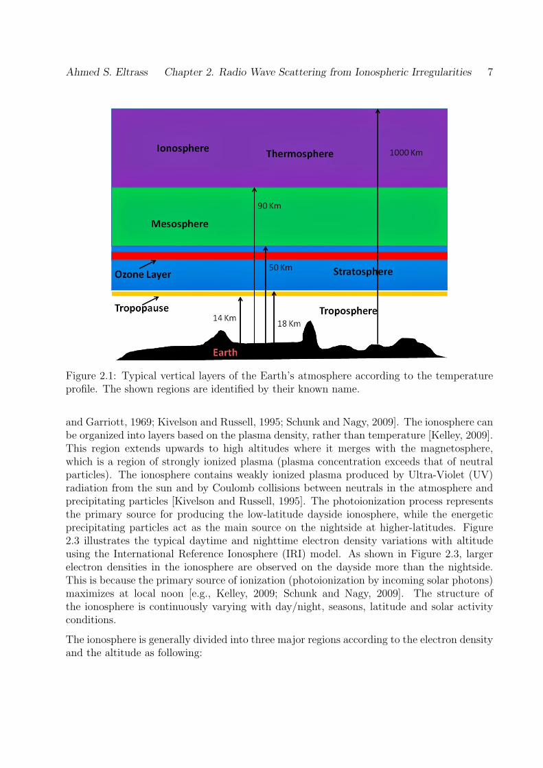
2.1 Typical vertical layers of the Earth’s atmosphere according to the temperatureprofile. The shown regions are identified by their known name. . . . . . . . . 7
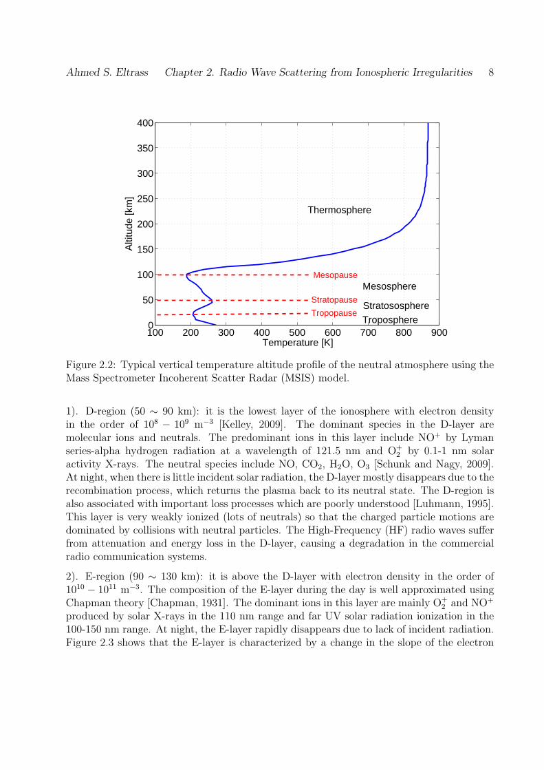
2.2 Typical vertical temperature altitude profile of the neutral atmosphere usingthe Mass Spectrometer Incoherent Scatter Radar (MSIS) model. . . . . . . 8
2.3 Typical plasma density altitude profile during the daytime (red) and the night-time (blue) generated from the IRI model. The ionosphere is divided into threeprincipal layers (from low to high: D, E, and F) according to the electron density. 9
2.4 Radio wave refraction in the ionosphere due to electron density fluctuations.Transmitted signals can be reflected back to the radar by ionospheric plasmairregularities (ionospheric scatter) or by the Earth’s surface (ground scatter). 16
2.5 A ray-tracing plot of HF radio waves during daytime (top) and nighttime(bottom) conditions for the Blackstone, VA radar. The ionosphere is color-coded by electron density using the 2011 IRI model. Gray lines represent thetransmitted radar rays, pink lines represent the Earth’s geomagnetic field lines,and white lines are regularly spaced slant-range intervals. The black markersare the regions of backscatter from either field-aligned plasma irregularities orthe Earth’s surface. . . . . . . . . . . . . . . . . . . . . . . . . . . . . . . . . 17
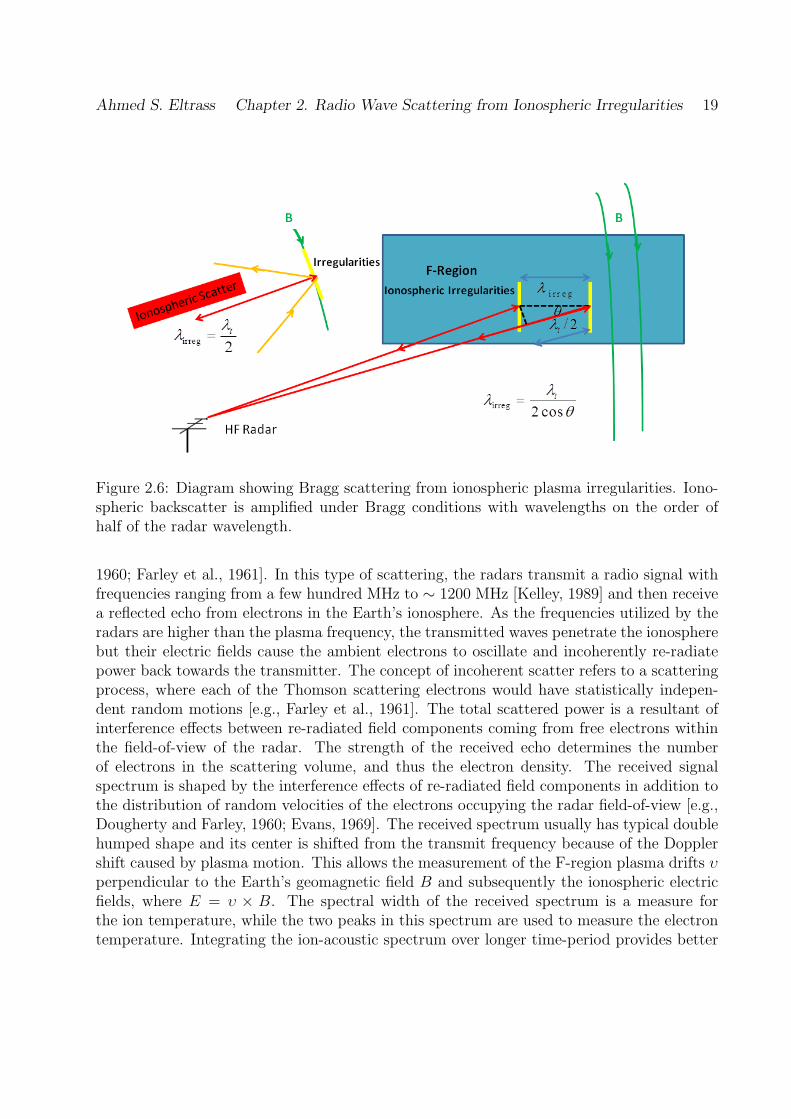
2.6 Diagram showing Bragg scattering from ionospheric plasma irregularities.Ionospheric backscatter is amplified under Bragg conditions with wavelengthson the order of half of the radar wavelength. . . . . . . . . . . . . . . . . . . 19
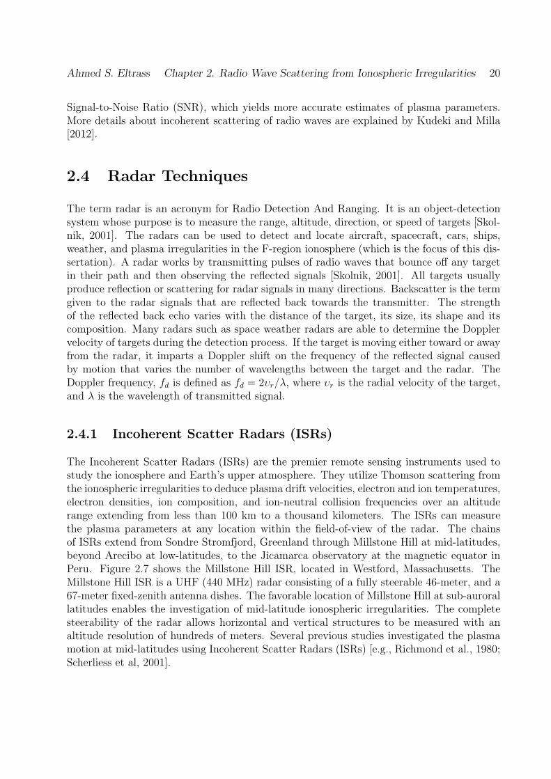
2.7 The Millstone Hill Incoherent Scatter Radar (ISR) located in Westford, Mas-sachusetts. This radar includes a 67 meter fixed-zenith antenna and a 46meter fully steerable antenna. . . . . . . . . . . . . . . . . . . . . . . . . . . 21
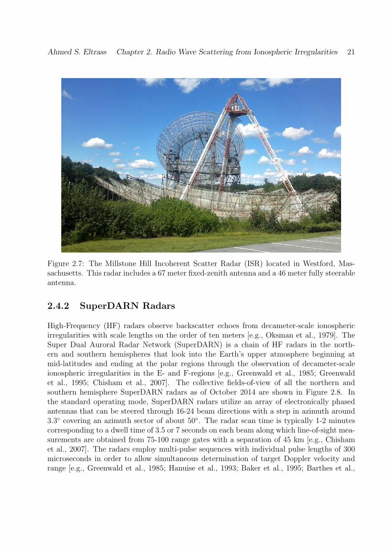
2.8 Fields of view of the SuperDARN radars in both hemispheres as of October2014. The right panel shows the southern hemisphere radars, and the leftpanel shows the northern hemisphere radars. Our work will be focused onmid-latitude (orange) radars in the northern hemisphere. . . . . . . . . . . . 22
ix
3.1 The physical mechanism of the TGI in the ionosphere (see text for details).The density and temperature gradients (κn and κT ), respectively, driving theTGI are assumed to be perpendicular to the magnetic field and oppositelydirected. . . . . . . . . . . . . . . . . . . . . . . . . . . . . . . . . . . . . . . 25
3.2 The TGI geometry relative to the magnetic field, the temperature gradient,the density gradient, and the wave vector of resistive drift waves. This geom-etry is also used for the GDI driven by diamagnetic and Pedersen drifts. . . . 27
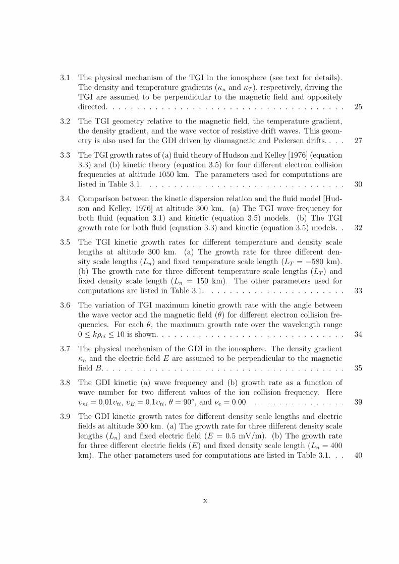
3.3 The TGI growth rates of (a) fluid theory of Hudson and Kelley [1976] (equation3.3) and (b) kinetic theory (equation 3.5) for four different electron collisionfrequencies at altitude 1050 km. The parameters used for computations arelisted in Table 3.1. . . . . . . . . . . . . . . . . . . . . . . . . . . . . . . . . 30
3.4 Comparison between the kinetic dispersion relation and the fluid model [Hud-son and Kelley, 1976] at altitude 300 km. (a) The TGI wave frequency forboth fluid (equation 3.1) and kinetic (equation 3.5) models. (b) The TGIgrowth rate for both fluid (equation 3.3) and kinetic (equation 3.5) models. . 32
3.5 The TGI kinetic growth rates for different temperature and density scalelengths at altitude 300 km. (a) The growth rate for three different den-sity scale lengths (Ln) and fixed temperature scale length (LT = −580 km).(b) The growth rate for three different temperature scale lengths (LT ) andfixed density scale length (Ln = 150 km). The other parameters used forcomputations are listed in Table 3.1. . . . . . . . . . . . . . . . . . . . . . . 33
3.6 The variation of TGI maximum kinetic growth rate with the angle betweenthe wave vector and the magnetic field (θ) for different electron collision fre-quencies. For each θ, the maximum growth rate over the wavelength range0 ≤ kρci ≤ 10 is shown. . . . . . . . . . . . . . . . . . . . . . . . . . . . . . . 34
3.7 The physical mechanism of the GDI in the ionosphere. The density gradientκn and the electric field E are assumed to be perpendicular to the magneticfield B. . . . . . . . . . . . . . . . . . . . . . . . . . . . . . . . . . . . . . . . 35
3.8 The GDI kinetic (a) wave frequency and (b) growth rate as a function ofwave number for two different values of the ion collision frequency. Hereυni = 0.01υti, υE = 0.1υti, θ = 90, and νe = 0.00. . . . . . . . . . . . . . . . 39
3.9 The GDI kinetic growth rates for different density scale lengths and electricfields at altitude 300 km. (a) The growth rate for three different density scalelengths (Ln) and fixed electric field (E = 0.5 mV/m). (b) The growth ratefor three different electric fields (E) and fixed density scale length (Ln = 400km). The other parameters used for computations are listed in Table 3.1. . . 40
x
3.10 The variation of TGI and GDI maximum kinetic growth rate with the anglebetween the wave vector and the magnetic field (θ). For each θ, the maximumgrowth rate over the wavelength range 0 ≤ kρci ≤ 10 is shown. . . . . . . . . 41
4.1 SuperDARN backscatter distribution between 00:00 and 05:00 UT on thenight of February 22-23, 2006. Beams 3 (left) and 9 (right) of the WallopsSuperDARN radar are highlighted in blue. Also shown is the position andpointing direction (black beam) of the Millstone Hill ISR during that night.The map is gridded with a geomagnetic coordinate system. . . . . . . . . . . 44
4.2 Backscatter observed by the Wallops SuperDARN radar on 22-23 February2006 from 22:00 to 05:00 UT in beam 9 (top 2 panels) and beam 3 (bottom2 panels). The backscatter power and Doppler velocities are shown for eachbeam. . . . . . . . . . . . . . . . . . . . . . . . . . . . . . . . . . . . . . . . 45
4.3 Summary of Millstone Hill ISR data on the night of 22-23 February 2006. (a)Electron densities at 300 km altitude for each pointing directions. (b) Electrontemperatures at 300 km altitude for each pointing directions. (c) Meridionalscale length for the electron density (black) and temperature (red) between53.8 and 58.1 magnetic latitude. Positive gradients (dashed) are polewardand up, while negative gradients (solid) are equatorward and down. . . . . . 46
4.4 Electron density (black curves) and electron temperature (red curves) scalelengths along (a) the meridional direction, (b) and the direction perpendicularto the geomagnetic field B. Positive gradients (dashed) are poleward and up,while negative gradients (solid) are equatorward and down. . . . . . . . . . . 47
4.5 The TGI and GDI geometry in the mid-latitude ionosphere relative to theEarth’s magnetic field, temperature and density gradient, diamagnetic andPedersen drifts, and the wave vector of resistive drift waves. The perpen-dicular temperature and density gradients are calculated as the sum of theprojections of the horizontal and vertical gradients (∇H and ∇V , respectively). 48
4.6 The TGI kinetic growth rate (equation 3.5) at altitude 300 km for differentelectron collision frequencies. The shown wavelength range 1.1 < kρci < 1.6corresponds to the operating frequency range of the Wallops SuperDARNradar throughout the experiment. . . . . . . . . . . . . . . . . . . . . . . . . 50
4.7 The time series of TGI and GDI growth rates for (a) meridional and (b)perpendicular scale lengths shown in Figure 4.4. The growth rates are calcu-lated over the wavelength range 1.1 < kρci < 1.6, which corresponds to theoperating frequency range of the Wallops SuperDARN radar throughout theexperiment. . . . . . . . . . . . . . . . . . . . . . . . . . . . . . . . . . . . . 51
xi
4.8 Backscatter echoes from the Blackstone SuperDARN radar on the nights ofOctober 15-16 and October 10-11, 2014. Backscatter power and line-of-sightDoppler velocity measured along beam 13 during the two events are shown inpanels (a, c) and (b, d), respectively. . . . . . . . . . . . . . . . . . . . . . . 55
4.9 Electron density (black curves) and electron temperature (red curves) scalelengths along the direction perpendicular to the geomagnetic field B dur-ing the nights of (a) October 15-16 and (b) October 10-11, 2014. Positivegradients (dashed) are poleward and up, while negative gradients (solid) areequatorward and down. . . . . . . . . . . . . . . . . . . . . . . . . . . . . . . 57
4.10 The time series of TGI and GDI growth rates on the nights of (a) October15-16 and (b) October 10-11, 2014. The growth rates are calculated overthe wavelength range 1.1 < kρci < 1.5, which corresponds to the operatingfrequency range of the Blackstone SuperDARN radar throughout the twoexperiments. . . . . . . . . . . . . . . . . . . . . . . . . . . . . . . . . . . . . 58
5.1 Time and space scales for different plasma simulation methods. . . . . . . . . 61
5.2 The gyro-kinetic TGI simulation geometry relative to the magnetic field, thetemperature and density gradients, and the wave vector of resistive drift waves.The temperature and density gradients are assumed to be opposite and per-pendicular to the magnetic field. . . . . . . . . . . . . . . . . . . . . . . . . . 65
5.3 The TGI (a) wave frequency and (b) growth rate of the kinetic dispersion re-lation (equation 3.5) at altitude 300 km. The parameters used for calculationsare listed in Table 3.1. . . . . . . . . . . . . . . . . . . . . . . . . . . . . . . 66
5.4 The geometric relationship of the gyro-kinetic method relative to the guidingcenter position (R), the actual particle position (x), and the gyro-radius (ρ). 67
5.5 Illustration of the gyro-averaging process, where ions are treated as chargerings and sampled at 4 spatial points [Lee, 1987]. (a) The gyro-averageddensity of a single ion particle is constructed by collecting charge density onthe grid points associated with the 4 shaded cells. (b) The electric field atguiding center is calculated from averaging at 4 points on the gyro-orbit. . . 68
5.6 The velocity vector scattering geometry. Two random angles Ψ and ϕ arecalculated to appropriately perform the change in the velocity vector due tocollisions. . . . . . . . . . . . . . . . . . . . . . . . . . . . . . . . . . . . . . 69
5.7 The normalized electrostatic field energy for three TGI simulations with vary-ing electron collision frequency. . . . . . . . . . . . . . . . . . . . . . . . . . 71
5.8 The normalized (a) electron heat flux and (b) electron diffusion coefficient fordifferent electron collision frequencies. . . . . . . . . . . . . . . . . . . . . . . 72
xii

5.9 Two-dimensional snapshots at t = 100/Ωci of (a) normalized electron densityand (b) electric potential wave number spectrum in the linear growth stage.In (a), the TGI waves propagate in the x-direction. In (b), the wave numberspectrum shows the TGI km-scale irregularities. . . . . . . . . . . . . . . . . 73
5.10 Two-dimensional snapshots at t = 1200/Ωci of (a) normalized electron densityand (b) electric potential wave number spectrum in the saturation stage. In(a), the nonlinearly enhanced density regions shown in the inset box are ofdecameter-scale (9-15 m). In (b), the wave number spectrum shows the TGIdecameter-scale irregularities. . . . . . . . . . . . . . . . . . . . . . . . . . . 74
5.11 The time evolution of the 1-D potential wave number spectrum, where P (kx)is the spatial power spectra averaged over the x-directions in arbitrary units.The spectral index of k−5.2 is calculated from the linear slope of potentialwave spectrum. . . . . . . . . . . . . . . . . . . . . . . . . . . . . . . . . . . 75
6.1 The GPS satellite constellation. The shown red lines represent the line-of-sight visible satellites for the ground GPS receiver. . . . . . . . . . . . . . . 79
6.2 Diagram showing the ionospheric refraction process that introduces propaga-tion delays on GPS signals. . . . . . . . . . . . . . . . . . . . . . . . . . . . 81
6.3 Diagram showing the radio wave propagation through a disturbed ionosphere.The ionospheric irregularities introduce phase shifts that become amplitudefluctuations as the wave propagates below the ionosphere. . . . . . . . . . . . 82
6.4 Coordinate system illustrating the radio wave propagation through a randomscattering medium (the ionosphere) [After Kintner et al., 2007]. . . . . . . . 84
6.5 S4 measurements for four different GPS satellites in view during the night of10-11 October 2014. . . . . . . . . . . . . . . . . . . . . . . . . . . . . . . . . 87
6.6 Phase scintillation measurements for two different GPS satellites in view dur-ing the night of 20-21 October 2014. . . . . . . . . . . . . . . . . . . . . . . 88
6.7 Power spectra of amplitude scintillation recorded at 04:50 UT on October 11,2014. The spectral index p and the Fresnel frequency fF are 2.8 and 0.09 Hz,respectively. The selected portion for estimating the spectral index is shownby two vertical dashed lines. . . . . . . . . . . . . . . . . . . . . . . . . . . . 91
6.8 Variation of spectral index (p) with amplitude scintillation index (S4) for scin-tillation measurements during January-December 2014. On average, the spec-tral index increases with increasing S4 index for weak to moderate amplitudescintillations. . . . . . . . . . . . . . . . . . . . . . . . . . . . . . . . . . . . 92
xiii
6.9 The power spectra for the DMSP F13-14 measurements of density irregular-ities as a function of spatial wave number during the shown periods on 26September 2001 [After Mishin and Blaunstein, 2008]. The spectral index ofk−1.8 is determined from the linear slope of the power spectra. . . . . . . . . 94
C.1 2-D simulation box set up with discretization of the plasma length. . . . . . 113
C.2 Computational cycle for the Particle-In-Cell (PIC) gyro-kinetic simulationmodel with collisional effects. . . . . . . . . . . . . . . . . . . . . . . . . . . 114
xiv
List of Tables
3.1 Parameters for computing the wave frequency and the growth rate of bothTGI and GDI at altitudes 1050 km and 300 km, respectively. . . . . . . . . . 31
4.1 The perpendicular and meridional electron temperature and density scalelengths computed at altitude 300 km on 22-23 February 2006. Ln and LT
are the density and temperature scale lengths, respectively. . . . . . . . . . . 49
5.1 Comparison of spectral indices for averaged power spectra of potential anddensity in Temperature Gradient Instability (TGI). . . . . . . . . . . . . . . 74
xv
Chapter 1
Introduction
The study of the near Earth space environment has become very essential due to its greatinfluence on the modern technologies and communication systems that directly affect ourtechnical infrastructure. The natural and artificial disturbances that may occur in the nearEarth space can produce disruptions on radio signals, including the Global Positioning Sys-tem (GPS), satellite communication systems, Over-The-Horizon (OTH) radars, HF commu-nications, and also influence global climate change [e.g., Baker, 2000]. Plasma instabilitiesand other magnetospheric sources can generate electron density fluctuations in the Earth’sionosphere, known as ionospheric irregularities, that impact the performance of various com-munication systems.
The ionospheric irregularities are small-scale structures in the ionospheric plasma densitycaused by plasma instability processes. The sources of plasma instabilities could be streamingvelocity of the particles relative to each other, inhomogeneities in the plasma density, densityand temperature gradients, electric fields, and anisotropies in plasma temperature [e.g., Fejerand Kelley, 1980; Keskinen and Ossakow, 1983]. Several processes such as the Perkinsinstability, the Gradient Drift Instability (GDI), and the Kelvin-Helmholtz instability werecited to identify the source of the ionospheric irregularities [e.g., Kelley and Miller, 1997;Ruohoniemi et al., 1988; Kelley, 2009]. These mechanisms lead to irregularities with scalesizes ranging from a few centimeters to several kilometers. According to their scale sizes,ionospheric irregularities can be monitored by a variety of techniques, both ground- andspace-based instruments that depend on various passive and active optical or electromagneticsystems [e.g., Schunk and Nagy, 2009]. Several previous studies have employed statisticalanalyses to identify the source of F-region irregularities [e.g., Ruohoniemi and Greenwald,1997; Milan et al., 1997; Ballatore et al., 2001; Parkinson et al., 2003; Koustov et al., 2004;Kane and Makarevich, 2010; Kumar et al., 2011; Ribeiro et al. 2012].
1
Ahmed S. Eltrass Chapter 1. Introduction 2
1.1 Motivation
Recent works indicate that the mid-latitude ionosphere is more active than currently ap-preciated, and that ionospheric processes producing the mid-latitude GPS scintillations areless understood due to lack of models and observations that can explain their characteristicsand distributions [e.g., Kelley, 2009]. During geomagnetically quiet conditions (Kp ≤ 2),the mid-latitude ionosphere (30 to 60 geomagnetic latitude) is a quiescent plasma but stillpopulated by plasma density irregularities generated by both plasma and neutral processes.The storm-time ionospheric irregularities at mid-latitudes are sufficiently strong to causesignal power fluctuations, known as ionospheric scintillation, in transionospheric satellitetransmissions such as GPS [e.g., Basu et al., 2001; Ledvina et al., 2002; Mishin et al., 2003].This raises the importance of knowing the cause and distribution of these ionospheric plasmairregularities to maintain the performance of satellite-ground data transmission. In this dis-sertation, we focus on the analysis and modeling of mid-latitude ionospheric irregularitiesand their impact on GPS scintillations.
The mid-latitude decameter-scale ionospheric irregularities with scale lengths on the orderof 10 m were studied early through the detection of backscatter echoes observed by High-Frequency (HF) radars [e.g., Oksman et al., 1979]. The Super Dual Auroral Radar Network(SuperDARN) consists of chains of HF radars that cover middle- and high-latitudes in bothhemispheres. SuperDARN radars monitor the ionospheric dynamics through the detectionof decameter-scale ionospheric plasma irregularities in the E- and F-regions [e.g., Green-wald et al., 1995; Chisham et al., 2007]. Oksavik et al. [2006] and Baker et al. [2007]have investigated the mid-latitude plasma dynamics during geomagnetically active periods.The mid-latitude SuperDARN radars have revealed decameter-scale ionospheric irregularitiesduring quiet geomagnetic periods that have been proposed to be responsible for the observedlow-velocity Sub-Auroral Ionospheric Scatter (SAIS) [e.g., Greenwald et al., 2006; Ribeiro etal., 2012; Kane et al., 2012]. Based on the coordination between the SuperDARN HF radarlocated at Wallops Island, Virginia and the Millstone Hill Incoherent Scatter Radar (ISR),Greenwald et al. [2006] reported recurring mid-latitude decameter-scale irregularities withlow drift velocities (< 100 m/s) during quiet geomagnetic periods on the nightside. Becauseof their low velocity, the GDI seemed an infeasible source for these irregularities and theyinstead suggested that the TGI [i.e., Hudson and Kelley, 1976] could be a feasible mechanismfor generating these irregularities. Using the data from the Blackstone, VA radar, Ribeiro etal. [2012] showed that the low-velocity SAIS associated with such irregularities is confinedto local night and is observed on 70 % of nights. Despite their high occurrence rate andlarge geographical spread, the plasma instability mechanism responsible for the growth ofthese irregularities is still unknown. A quantitative analysis of growth rates and timescalesof feasible plasma instabilities is required to identify what mechanisms predominate.
Several studies have focused on the space weather impacts in the mid-latitude sub-auroralionosphere during magnetic storm periods [e.g., Foster et al., 2002; Mishin et al., 2003; Basuet al., 2001; Ledvina et al., 2002]. During disturbed geomagnetic conditions, large regions
Ahmed S. Eltrass Chapter 1. Introduction 3
hosting an ionospheric density gradient exist in the evening sector at sub-auroral latitudesin the top-side ionosphere [e.g., Coster et al., 2005; Spiro et al., 1979; Evans et al., 1983;Anderson et al., 1991, 1993]. These density gradients are often associated with streams ofenhanced plasma convection known as Sub-Auroral Plasma Streams (SAPS) [e.g., Fosterand Burke, 2002], and with Storm-Enhanced Densities (SEDs) [e.g., Erickson et al., 2002].Satellite and radar observations reveal that the SAPS region is often irregular and includeswave-like structures [e.g., Erickson et al., 2002; Mishin et al., 2002, 2003, 2004; Streltsovand Mishin, 2003]. Mishin and Blaunstein [2008] showed that intense mid-latitude UHFand L1-band scintillations observed by Basu et al. [2001, 2008] and Ledvina et al. [ 2002]originated within structured SAPS. Strong SAPS wave structures and irregular plasma den-sity troughs are associated with strong temperature and density gradients, quite similar tothe observations of Mishin et al. [2003, 2004]. The generation mechanism of such strongoppositely directed gradients has been suggested by Mishin and Burke [2005] inside the plas-masphere and by Mishin [2013] at the plasmapause. It is due to strong electron heating inthe plasmasphere by plasma turbulence generated by hot plasma jets penetrating from themagnetotail. Then, heat transport leads to heating of ionospheric electrons and formationof the plasma density troughs. Using satellite data from the Defense Meteorological SatelliteProgram (DMSP), Mishin et al. [2003] determined that small-scale density, electric field,velocity, and electron temperature structures can occur in SAPS storm-time mid-latitudetrough structures. Keskinen et al. [2004] suggested that the Temperature Gradient Insta-bility (TGI) in association with the Gradient Drift Instability (GDI) could be responsiblefor generating these small-scale structures in the trough wall region. Although the TGI andGDI are suggested to be responsible for the observed mid-latitude ionospheric irregularities,more detail is not known about the exact role of these plasma instabilities in generatingthe sub-auroral irregularities [e.g., Kelley, 2009]. Important effects to be considered in fur-ther detail include different spatial scales, nonlinear cascading, and the impact of E-regionconductance.
1.2 Research Objectives
The aim of this work is to model and analyze the observed ionospheric structures at mid-latitudes through the coordination between the SuperDARN HF radars, Incoherent ScatterRadars (ISRs), and GPS receivers under various sets of geomagnetic conditions. This canbe achieved by determining the role of the Temperature Gradient Instability (TGI) and theGradient Drift Instability (GDI) in the generation of these ionospheric irregularities. Thelinear theory of both TGI and GDI are extended into the kinetic regime appropriate forHF radar frequencies and analyzed as the cause of these irregularities. Although the lineartheory provides the insight for the initial growth, it cannot describe the subsequent nonlin-ear evolution and the associated particle transport. To investigate such nonlinear effects,the gyro-kinetic simulation model, which contains the nonlinearities relevant to F-regionirregularities, is employed. The usefulness of gyro-kinetic particle simulation as a computa-
Ahmed S. Eltrass Chapter 1. Introduction 4
tional tool is demonstrated to allow the study of the nonlinear evolution and the saturationmechanisms of the TGI for the observed decameter-scale ionospheric irregularities. Multipledata sets from dual frequency GPS receivers at Virginia Tech University and MIT HaystackObservatory are analyzed to study the amplitude and phase fluctuations of the received sig-nals and to investigate the spectral index variations of GPS scintillations due to ionosphericirregularities. The GPS measurements show that L-band scintillations occur more oftenthan previously thought, however, intense scintillations may be so exacting that only rareoccurrences are possible. The GPS spectral indices are calculated and compared with bothsimulation results and previous in-situ satellite measurements. The reasonable agreementbetween experimental, theoretical, and computational results of this study suggests that aTGI turbulent cascade may cause the quiet-time decameter-scale size irregularities, whileturbulent cascade processes of both TGI and GDI are responsible for the disturbed-timeirregularities that may cause GPS scintillations. The broad objectives of this research workcan be summarized as following:
1. Investigate the physical mechanism of the Temperature Gradient Instability (TGI) andextend the linear theory of both TGI and GDI into the kinetic regime appropriate for HFradar frequencies. The TGI and GDI calculations are obtained over a broad set of parameterregimes to underscore limitations in fluid theory for decameter-scale waves.
2. Investigate co-located observations by Incoherent Scatter Radars (ISRs) and SuperDARNHF radars at mid-latitudes under various sets of geomagnetic conditions to identify thephysical mechanisms responsible for the observed ionospheric plasma irregularities. A criticalcomparison of TGI and GDI is made for different observations in the sub-auroral ionosphereby the development of the growth rate time series of both TGI and GDI.
3. Study the nonlinear evolution of the mid-latitude ionospheric TGI utilizing gyro-kineticParticle-In-Cell (PIC) simulation techniques with Monte Carlo collisions for the first time.The purpose of this investigation is to identify the mechanism responsible for the nonlinearsaturation as well as the associated anomalous transport. The spatial power spectra ofthe electrostatic potential and density fluctuations associated with the TGI are computed todetermine the important consequences of the TGI nonlinear evolution such as wave cascading.This is critical for ultimately determining the scale size of the irregularities observed by theradar observations.
4. Investigate the potential impact of ionospheric irregularities on GPS signals utilizingdata collected from GPS stations at mid-latitudes. The scintillation data are analyzed tomonitor the amplitude and phase scintillations and to obtain the spectral characteristics ofirregularities producing ionospheric scintillations at mid-latitudes. A cascade product fromboth TGI and GDI is suggested to be responsible for the mid-latitude irregularities thatcause GPS scintillations during disturbed geomagnetic conditions.
Ahmed S. Eltrass Chapter 1. Introduction 5
1.3 Dissertation Organization
The dissertation is organized as follows. Chapter 2 presents a review of the Earth’s upperatmosphere and the radio wave scattering in the ionosphere due to plasma wave instabilitiesrelevant for this study. Also, Chapter 2 introduces the SuperDARN radars and the IncoherentScatter Radars (ISRs) that will be used to study the plasma wave irregularities at mid-latitudes. Chapter 3 presents the fluid and kinetic models of both the Temperature GradientInstability (TGI) and the Gradient Drift Instability (GDI). In this chapter, the TGI and GDIcalculations are obtained over a wide range of parameters to underscore limitations in fluidtheory for short wavelengths and to provide perspective on the experimental observationsin next chapter. Chapter 4 illustrates the co-located experimental observations by the mid-latitude SuperDARN radars and the Millstone Hill ISR under various sets of geomagneticconditions. Next, a critical comparison of TGI and GDI is made for these observations bythe development of the growth rate time series of both TGI and GDI. In Chapter 5, thenonlinear gyro-kinetic simulation algorithm is described in order to define the system underinvestigation and the basic gyro-kinetic formalism for studying the TGI. Next, Chapter 5presents the simulation results over a broad set of parameter regimes to investigate thenonlinear behavior including saturation amplitude and mechanisms. The discussion of thesimulation results corresponding to SuperDARN observations is also presented. Chapter 6addresses the potential impact of the mid-latitude ionospheric irregularities on GPS signals.Next, the spectral characteristics of the density fluctuations associated with ground GPSscintillations are calculated and compared with both simulation results and previous in-situsatellite spectral measurements. Chapter 7 outlines conclusions and recommendations forfuture work. Finally, the simplified approximations of the TGI kinetic dispersion relation,the numerical analysis of instability kinetic dispersion relations, and the description of the2-D electrostatic gyro-kinetic simulation model are presented in further detail in AppendicesA, B and C, respectively.
Chapter 2
Radio Wave Scattering fromIonospheric Irregularities
This chapter provides an overview of the Earth’s upper atmosphere, plasma instability pro-cesses, and the radio wave scattering from the ionospheric density fluctuations relevant tothis investigation. This chapter also presents the radars that will be used to investigate theionospheric wave-like structures.
2.1 The Ionosphere
2.1.1 Basic Structure and Formation
The Earth’s atmosphere is typically divided in vertical layers based on its neutral charac-teristic temperature regime [e.g., Kelley, 2009]. As shown in Figure 2.1, the atmosphere isarranged in 4 layers: troposphere (0-10 km), stratosphere (10-50 km), mesosphere (50-90km), and thermosphere (above 90 km). Figure 2.2 illustrates a representative temperatureprofile for the layers of the neutral atmosphere. With the altitude increase, the temperaturefalls through the troposphere, rises through the stratosphere, falls again through the meso-sphere, and finally rises through the thermosphere. Each layer is bounded by a pause wherethe temperature reaches a minimum (tropopause, mesopause) or a maximum (stratopause).As shown in Figure 2.2, the topmost layer of the atmosphere (thermosphere) is characterizedby a significant temperature increase with altitude due to the effect of solar radiation. Thiscauses the neutral gas in the upper atmosphere to be weakly ionized, forming a region ofcold plasma, known as the ionosphere, which extends from 50 to 1000 km.
The Earth’s ionosphere is the region of the atmosphere that stretches approximately between50 km to the edge of space at around 1000 km above the surface of the Earth [e.g., Rishbeth
6
Ahmed S. Eltrass Chapter 2. Radio Wave Scattering from Ionospheric Irregularities 7
Figure 2.1: Typical vertical layers of the Earth’s atmosphere according to the temperatureprofile. The shown regions are identified by their known name.
and Garriott, 1969; Kivelson and Russell, 1995; Schunk and Nagy, 2009]. The ionosphere canbe organized into layers based on the plasma density, rather than temperature [Kelley, 2009].This region extends upwards to high altitudes where it merges with the magnetosphere,which is a region of strongly ionized plasma (plasma concentration exceeds that of neutralparticles). The ionosphere contains weakly ionized plasma produced by Ultra-Violet (UV)radiation from the sun and by Coulomb collisions between neutrals in the atmosphere andprecipitating particles [Kivelson and Russell, 1995]. The photoionization process representsthe primary source for producing the low-latitude dayside ionosphere, while the energeticprecipitating particles act as the main source on the nightside at higher-latitudes. Figure2.3 illustrates the typical daytime and nighttime electron density variations with altitudeusing the International Reference Ionosphere (IRI) model. As shown in Figure 2.3, largerelectron densities in the ionosphere are observed on the dayside more than the nightside.This is because the primary source of ionization (photoionization by incoming solar photons)maximizes at local noon [e.g., Kelley, 2009; Schunk and Nagy, 2009]. The structure ofthe ionosphere is continuously varying with day/night, seasons, latitude and solar activityconditions.
The ionosphere is generally divided into three major regions according to the electron densityand the altitude as following:
Ahmed S. Eltrass Chapter 2. Radio Wave Scattering from Ionospheric Irregularities 8
100 200 300 400 500 600 700 800 9000
50
100
150
200
250
300
350
400
Temperature [K]
Alti
tude
[km
]
Stratopause
Mesopause
TroposphereTropopause
Stratososphere
Mesosphere
Thermosphere
Figure 2.2: Typical vertical temperature altitude profile of the neutral atmosphere using theMass Spectrometer Incoherent Scatter Radar (MSIS) model.
1). D-region (50 ∼ 90 km): it is the lowest layer of the ionosphere with electron densityin the order of 108 − 109 m−3 [Kelley, 2009]. The dominant species in the D-layer aremolecular ions and neutrals. The predominant ions in this layer include NO+ by Lymanseries-alpha hydrogen radiation at a wavelength of 121.5 nm and O+
2 by 0.1-1 nm solaractivity X-rays. The neutral species include NO, CO2, H2O, O3 [Schunk and Nagy, 2009].At night, when there is little incident solar radiation, the D-layer mostly disappears due to therecombination process, which returns the plasma back to its neutral state. The D-region isalso associated with important loss processes which are poorly understood [Luhmann, 1995].This layer is very weakly ionized (lots of neutrals) so that the charged particle motions aredominated by collisions with neutral particles. The High-Frequency (HF) radio waves sufferfrom attenuation and energy loss in the D-layer, causing a degradation in the commercialradio communication systems.
2). E-region (90 ∼ 130 km): it is above the D-layer with electron density in the order of1010 − 1011 m−3. The composition of the E-layer during the day is well approximated usingChapman theory [Chapman, 1931]. The dominant ions in this layer are mainly O+
2 and NO+
produced by solar X-rays in the 110 nm range and far UV solar radiation ionization in the100-150 nm range. At night, the E-layer rapidly disappears due to lack of incident radiation.Figure 2.3 shows that the E-layer is characterized by a change in the slope of the electron

Ahmed S. Eltrass Chapter 2. Radio Wave Scattering from Ionospheric Irregularities 9
106
108
1010
1012
1014
10
100
1000
Plasma Density (electrons/m3)
Alti
tude
(km
)
NightDay
F−RegionF2−Region
F1−Region
Night Day
E−RegionD−Region
Figure 2.3: Typical plasma density altitude profile during the daytime (red) and the night-time (blue) generated from the IRI model. The ionosphere is divided into three principallayers (from low to high: D, E, and F) according to the electron density.
density profile at ∼ 100 km altitude. A region of enhanced ionization and high electrondensity called the Sporadic E-region is often observed at mid-latitudes in the lower E-regionat altitudes between 95-120 km [Hargreaves, 1979]. The E-region can only reflect incidentradio waves of frequencies less than 10 MHz and may cause absorption for frequencies above.
3). F-region (above ∼ 130 km): it is the region of peak plasma density in the ionospherethat extends above about 130 km altitude with electron density in the order of 1011 − 1012
m−3 (see Figure 2.3). Since two plasma density peaks can occur in the F-region, it is oftenfurther divided into F1- and F2-regions as following:
a). F1-region (150 ∼ 200 km): it is composed of a mixture of molecular ions O+2 and NO+,
and dominated by atomic ions O+ produced by Extreme Ultra-Violet (EUV) radiation inthe 10-100 nm range. The F1-layer is controlled by photochemistry resulted from the pres-ence of molecular ions, and thus it is well approximated as a Chapman layer like the E-region.
Ahmed S. Eltrass Chapter 2. Radio Wave Scattering from Ionospheric Irregularities 10
b). F2-region (> 200 km): it is the region of the ionosphere with the highest electrondensity up to 1012 m−3 (see Figure 2.3). The F2-region consists primarily of ionized atomicOxygen (O+) and Nitrogen (N+). The F2 density peak (hmF2) is the peak density forthe entire ionosphere and it occurs between 250 km and 400 km altitude. The Chapmantheory is not suitable for modeling the F2-region because this layer is controlled not only byrecombination but also by diffusion and vertical transport processes [Luhmann, 1995]. TheF-region plasma density does not drop steeply at night like other layers because (1) the O+
has longer recombination time constant, and (2) vertical transport processes allow plasmato flow from the plasmasphere into the F-region ionosphere during nighttime, and thusmaintain the plasma density [Kelley, 2009]. The F-layer with the maximum plasma densityprovides the possibility for long distance radio communication through the refraction of HFradio waves in the F-region. This represents the basis for sky wave propagation, HF radiocommunications over long distances, and for Over-The-Horizon (OTH) radar.
According to the changing orientation of geomagnetic field lines with latitude, the iono-sphere can be structured into low-latitude (equatorial), mid-latitude (sub-auroral), andhigh-latitude (auroral) regions. The low-latitude region is characterized by nearly horizontalgeomagnetic field while the high-latitude region is defined by the energetic particle precip-itation. The mid-latitude region (which is the focus of this study) is usually considered asan intermediary zone with effects from both high- and low-latitude processes [Kelley, 2009].
2.1.2 The Mid-Latitude Ionosphere
The mid-latitude ionosphere behaves as a buffer zone between low-latitude (equatorial) re-gions and high-latitude (auroral) regions, with boundaries that change with the variationsof the geomagnetic activity [Kelley, 2009]. Recent studies reveal that the mid-latitude re-gion is more complicated than previously thought, as it includes many different scales ofwave-like structures [e.g., Kelley, 2009]. During geomagnetically quiet conditions (Kp ≤ 2),the mid-latitude ionosphere (30 to 60 geomagnetic latitude) is a quiescent plasma but stillpopulated by plasma density irregularities generated by both plasma and neutral processes[e.g., Titheridge, 1995; Tsugawa et al., 2007]. The plasma instability mechanism responsiblefor the growth of these irregularities is still unknown. The magnetospheric electric fields donot have a large effect on the quiet-time mid-latitude ionosphere due to the shielding effectof the Alfven layers [e.g., Huba et al., 2005]. The storm-time ionospheric irregularities atmid-latitudes are sufficiently strong to cause signal power fluctuations, known as ionosphericscintillation, in transionospheric satellite transmissions such as the Global Positioning Sys-tem (GPS) [e.g., Basu et al., 2001; Ledvina et al., 2002; Mishin et al., 2003]. This raisesthe importance of knowing the cause and distribution of these ionospheric plasma irregular-ities (which is the focus of this study) to maintain the performance of satellite-ground datatransmission.
Ahmed S. Eltrass Chapter 2. Radio Wave Scattering from Ionospheric Irregularities 11
2.2 Plasma Instability Processes
2.2.1 Plasma Concepts
A plasma is a quasi-neutral gas of charged and neutral particles (electrons and ions) whichexhibits a collective behavior. The basic plasma concepts can be summarized through thefollowing parameters:
1). Plasma frequency: consider two species of charged particles in a plasma, electrons andpositively charged ions. If the electrons in a plasma are displaced from a uniform backgroundof ions, electric fields will be formed such that the Coulomb forces pull the electrons backto their original positions in order to restore the charge neutrality. Due to their inertia, theelectrons will overshoot and oscillate around their equilibrium positions with a frequency,known as the plasma frequency. Since the ion mass is much smaller than the electron mass,the ions do not have time to respond to the oscillation field of electrons. The electron plasmafrequency is given by:
ωp =
√q2en0
meϵ0(2.1)
where, ωp is the electron plasma frequency, ϵ0 is the permittivity of free space, and qe, n0,me are the charge, charge density, and the mass of the electrons, respectively. A convenientapproximate formula for electron plasma frequency is
fp = 9√n0 (2.2)
where, fp is the electron plasma frequency in Hz. At the F-region ionosphere, where n0 ∼ 1012
m−3, the corresponding plasma frequency is fp ∼ 9 MHz.
2). Cyclotron frequency: if a magnetic field is applied on a charged particle, the particleundergoes a helix motion (gyro-motion) along the magnetic field with a frequency, known asthe cyclotron frequency. The cyclotron frequency (gyro-frequency) is given by:
Ωc =qB
m(2.3)
where, Ωc is the cyclotron frequency and B is the applied magnetic field strength. The radiusof gyration ρc = υt/Ωc is called the Larmor radius or the gyro-radius, where υt is the thermalvelocity.
3). Velocity distribution function: it describes the fact that particles in a plasma do notmove at the same velocity. In equilibrium, the velocity distribution function is Maxwellian.The 1-D Maxwellian distribution function is given by:
Ahmed S. Eltrass Chapter 2. Radio Wave Scattering from Ionospheric Irregularities 12
f(v) =n√πυt
exp(−υυ2t
) (2.4)
υt =√kBT/m is the species thermal velocity, kB is the Boltzmann constant, and n is the
plasma density. The thermal velocity represents a measure for the spread in the velocitydistribution function.
Several plasma characteristics could be obtained from the velocity distribution functionsuch as the plasma density and the average particle kinetic energy. When the distributionof particle velocities departs from the Maxwellian thermodynamic equilibrium and exhibitsdistinctly non-thermal features, plasma waves may grow through plasma instability processes(which will be explained shortly).
4). Debye length: it is one of the most important length scales in the plasma as it representsa measure for the plasma shielding distance. When external potentials are introduced intoa plasma, they are shielded. The Debye length is essentially the length over which thepotential of isolated charges are screened in a plasma (i.e., the thickness of the electronscreening cloud). The Debye length is given by:
λD =
√ϵ0kBTenqe
(2.5)
where, kB is the Boltzmann constant and Te is the electron temperature. Note that classifyingthe plasma as a quasi-neutral gas means that the plasma is neutral enough to assume ni =ne = n, where n is the plasma density.
A Debye sphere is a volume whose radius is the Debye length, in which charges outside thesphere are electrically screened [Chen, 1984]. The concept of Debye shielding is only valid ifthere are enough particles in the Debye sphere. The number of particles ND in the Debyesphere is given by [Chen, 1984]:
ND = n4
3πλ3D (2.6)
At the F-region ionosphere, where T ∼ 1000 K and n ∼ 1012 m−3, the corresponding Debyelength is ∼ 2.2 mm and ND ∼ 4.3× 10⁴.
The preceding parameters provide the conditions that must be satisfied in any ionized gasto be classified as a plasma:
• It has to be large enough that the size of the plasma is larger than the Debye length,L >> λD.
Ahmed S. Eltrass Chapter 2. Radio Wave Scattering from Ionospheric Irregularities 13
• The number of charged particles in the Debye sphere is large enough to make the Debyeshielding statistically valid, ND >> 1.
• The collisional frequency between the charged and neutral particles is smaller than thenatural plasma frequency ωp such that ωpτ > 1, where τ is the mean free time betweencollisions.
Since the ionosphere satisfies the aforementioned three conditions, it can be treated as aplasma. The collective particle motion in the ionosphere under the influence of electromag-netic or electrostatic fields can be treated as following:
1). Fluid theory: it is the simplest description of a plasma because it treats the plasmaas a moving fluid that is affected by electric and magnetic field forces. The fluid theoryneglects the identity of individual particles and only the motion of fluid elements as a wholeis taken into account. It also neglects the velocity-dependent efforts such as the Landaudamping and wave-particle effects. Fluid models allow the plasma formulation in termsof a dielectric response function as in standard electromagnetics. The fluid treatment forionospheric plasma is appropriate for the long wavelength regime (λ >> 15 m), however,it looses validity in the short wavelength, which is where kinetic effects begin to play animportant role.
2). Kinetic theory: it is the most accurate description of a plasma. The kinetic theory shouldbe used when particles cannot be approximated as all moving at the same speed, i.e., thevelocity distribution should be known. In this case, the plasma velocity distribution functionis used to describe the motion under the influence of electric and magnetic forces. One of themost important physical processes that is described by kinetic theory is the wave-particleinteraction, which can cause damping for the plasma waves and temperature increase forthe particles. This phenomena can also lead to velocity reduction for the resonant particles.The kinetic treatment for ionospheric plasma must be used for short wavelengths (λ ≤ 15m)as the fluid theory breaks down for this wavelength regime.
2.2.2 Plasma Waves
If a plasma contains a certain form of free energy in the particles, this free energy causesthe plasma waves to grow until they reach the steady state, which brings the system backinto equilibrium. Identification of the free energy source is essential to understand a givenplasma wave because distinct free energy sources may lead to very different consequences.Plasma waves which produce plasma instabilities can be categorized as electromagnetic orelectrostatic according to whether or not there is an oscillating magnetic field. Plasma wavescan be further classified by the oscillating species (electron and ion waves). The variouswave modes can also be classified according to whether they propagate in an unmagnetizedplasma or parallel, perpendicular, or oblique to the stationary magnetic field. The plasmawave modes and plasma instabilities in the linear regime can be described by a specific
Ahmed S. Eltrass Chapter 2. Radio Wave Scattering from Ionospheric Irregularities 14
relationship between frequency and wave number. This is called a dispersion relation and ithas the following form:
ω = ωr(k) + iωi(k) (2.7)
where, ωr is the wave frequency and ωi = γ is the growth rate. Important characteristicsfor plasma waves could be obtained from the dispersion relation such as the phase velocityυp = ω/k and the group velocity υg = ∂ω/∂k. If the frequency is complex and ωi = γ > 0,then this describes a growing wave mode or plasma instability, where the growth rate involvesnonlinear and kinetic effects. The wave growth often leads to a situation where some plasmaparticles start to interact with the growing wave, e.g., by heating. This can be explained interms of the so-called quasi-linear saturation within the Vlasov theory.
The plasma instability is a region where turbulence occurs due to changes in the character-istics of a plasma (e.g., temperature, density, electric fields, magnetic fields). The plasmainstabilities could be classified according to the type of free energy from which they arederived as following:
1). Streaming instabilities: these instabilities derive their energy from the streaming velocityof the particles relative to each other.
2). Configuration instabilities: they are generated due to inhomogeneities in the plasma den-sity, electric field flow velocity, pressure, temperature gradients, electric fields, and anisotropiesin plasma temperature.
3). Kinetic instabilities: they are derived by the deviation of the plasma velocity distributionfrom the Maxwellian distribution, i.e., the particles in a plasma do not move at the samevelocity. This can also be related as streaming instabilities.
2.2.3 Ionospheric Plasma Instabilities
Plasma instability processes can produce irregularities or turbulence in the ionosphere thatcause small-scale structures in the plasma density. Several plasma instabilities were wellstudied to identify the source of the ionospheric irregularities in high-latitude and equatorialregions [e.g., Kelley, 2009]. At low-latitudes, the combined effects of gravity and an eastwardelectric fields, in the presence of a vertical upward density gradient, can excite a plasmainstability known as Rayleigh-Taylor instability. The Rayleigh-Taylor instability typicallyforms the equatorial F-region irregularities, where the magnetic field is nearly perpendicularto the gravitational field [e.g., Dungey, 1956; Basu et al., 1978; Tsunoda, 1981; Kelley,1989]. The growth of Rayleigh-Taylor instability causes plume-like structure in electrondensity distribution (ionospheric bubbles) with scales ranging from 10 to 100 km [e.g., Basuet al., 1983]. Such structures produce equatorial plasma turbulence that may cause intenseamplitude and phase fluctuations for radio waves. The equatorial E-region irregularities are

Ahmed S. Eltrass Chapter 2. Radio Wave Scattering from Ionospheric Irregularities 15
strongly correlated with the equatorial electrojet, which is more intense over the magneticequator. The east-west drift velocity of the electrons exceeds the ion-acoustic speed, allowingthe growth of the two-stream instability. The echoes from this type of instabilities arecharacterized by a narrow spectrum with a doppler shift that corresponds approximately tothe ion acoustic velocity in the electrojet region. Another instability process that is knownto cause irregularities in the high- and low-latitudes is the Kelvin-Helmholtz or velocity-shear driven instability [e.g., Keskinen et al., 1988; Kintner and Seyler, 1985]. The Kelvin-Helmholtz instability is generated due to sheared (or inhomogeneous) E × B velocity flowsin plasma caused by inhomogeneous electric field. This instability produces turbulence inthe form of vortices (vortical structures) and leads to ionospheric irregularities at high- andlow-latitudes.
The low- and high-latitude plasma wave irregularities have been studied in detail for manydecades. In contrast, the mid-latitude plasma instability mechanisms are less understooddue to lack of models and observations that can explain the characteristics of these instabil-ities. In the context of this dissertation, we restrict our interest to the mid-latitude plasmainstabilities and their potential role in generating the ionospheric irregularities.
2.3 Radio Wave Scattering
Radio waves scatter and reflect in the ionosphere based on frequencies, polarizations, andionospheric conditions. The presence of free electrons in the ionosphere plays an importantrole in the radio wave propagation over a wide band of frequencies from 3 KHz to 30 GHz.When a radio wave reaches the ionosphere, the alternating electric field in the wave causesthe free electrons to move with the same frequency as the radio wave. The proximity ofthe transmitted signal to the plasma frequency determines what fraction of the transmittedsignal is refracted, reflected, transmitted or absorbed. Figure 2.4 illustrates the differentpossibilities for radio wave propagation through the ionosphere. If the transmitted frequencyis higher than the plasma frequency, the electrons are unable to respond fast enough andthey cannot re-radiate the signal, while waves with lower frequencies than plasma frequencyreflect from either plasma irregularities in the E- and F-regions or the Earth’s surface.
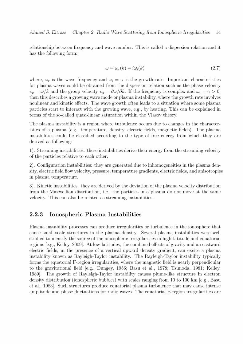
High-Frequency (HF, 10-20 MHz) radars utilize radio wave refraction in the ionosphere toobserve two types of backscatter:1). Ionospheric scatter: the ionospheric scatter produced by plasma instabilities in theE- and F-regions is observed when the radar wave vector k is nearly orthogonal to thegeomagnetic field B, a criterion known as the aspect condition. The HF refraction in theF-region ionosphere is utilized to bend the radio signals such that the waves propagate nearlyhorizontally and thus perpendicular to the geomagnetic field lines. This will maximize thecross section for the refraction from the field-aligned ionospheric irregularities [e.g., Hysellet al., 1996]. This is illustrated in Figures 2.4 and 2.6.
Ahmed S. Eltrass Chapter 2. Radio Wave Scattering from Ionospheric Irregularities 16
Figure 2.4: Radio wave refraction in the ionosphere due to electron density fluctuations.Transmitted signals can be reflected back to the radar by ionospheric plasma irregularities(ionospheric scatter) or by the Earth’s surface (ground scatter).
2). Ground scatter: the ground backscatter is observed when radar rays are refracted backto the Earth’s surface, resulting in backscatter from the ground to the radar according toterrain (geometry, composition) [e.g., Ponomarenko et al., 2010]. This type of scatter ischaracterized by the skip focusing distance (see Figure 2.4), which is defined as the closestregion where rays reach the ground after reflection in the ionosphere. The ground scatter isoften perturbed by gravity waves, changes in electron density, neutral winds, and TravellingIonospheric Disturbances (TIDs) [e.g., Samson et al., 1989; Bristow et al., 1996].
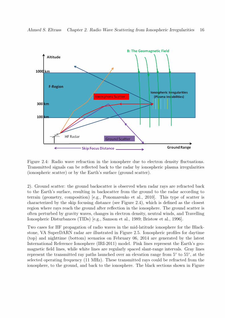
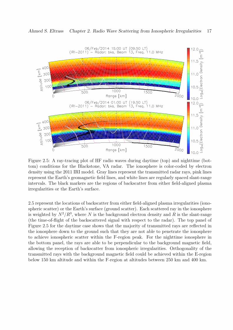
Two cases for HF propagation of radio waves in the mid-latitude ionosphere for the Black-stone, VA SuperDARN radar are illustrated in Figure 2.5. Ionospheric profiles for daytime(top) and nighttime (bottom) scenarios on February 06, 2014 are generated by the latestInternational Reference Ionosphere (IRI-2011) model. Pink lines represent the Earth’s geo-magnetic field lines, while white lines are regularly spaced slant-range intervals. Gray linesrepresent the transmitted ray paths launched over an elevation range from 5 to 55, at theselected operating frequency (11 MHz). These transmitted rays could be refracted from theionosphere, to the ground, and back to the ionosphere. The black sections shown in Figure
Ahmed S. Eltrass Chapter 2. Radio Wave Scattering from Ionospheric Irregularities 17
Figure 2.5: A ray-tracing plot of HF radio waves during daytime (top) and nighttime (bot-tom) conditions for the Blackstone, VA radar. The ionosphere is color-coded by electrondensity using the 2011 IRI model. Gray lines represent the transmitted radar rays, pink linesrepresent the Earth’s geomagnetic field lines, and white lines are regularly spaced slant-rangeintervals. The black markers are the regions of backscatter from either field-aligned plasmairregularities or the Earth’s surface.
2.5 represent the locations of backscatter from either field-aligned plasma irregularities (iono-spheric scatter) or the Earth’s surface (ground scatter). Each scattered ray in the ionosphereis weighted by N2/R3, where N is the background electron density and R is the slant-range(the time-of-flight of the backscattered signal with respect to the radar). The top panel ofFigure 2.5 for the daytime case shows that the majority of transmitted rays are reflected inthe ionosphere down to the ground such that they are not able to penetrate the ionosphereto achieve ionospheric scatter within the F-region peak. For the nighttime ionosphere inthe bottom panel, the rays are able to be perpendicular to the background magnetic field,allowing the reception of backscatter from ionospheric irregularities. Orthogonality of thetransmitted rays with the background magnetic field could be achieved within the E-regionbelow 150 km altitude and within the F-region at altitudes between 250 km and 400 km.
Ahmed S. Eltrass Chapter 2. Radio Wave Scattering from Ionospheric Irregularities 18
2.3.1 Bragg Scattering
When the radar signal hits small-scale electron density irregularities, the signal will returndirectly to the radar only when the transmitted signal scatters off a plasma wave that is on theorder of half the transmitted wavelength, and that is traveling in a radial path either directlyaway from or towards the radar. The backscattered electromagnetic waves are generated byfree electrons in the ionosphere accelerated by a transmitted signal, resulting in a strongreturn of energy at a very precise wavelength. This is known as the Bragg scattering. Asshown in Figure 2.6, the irregularity wavelength can be expressed as
λirreg =λt
2cos(θ)(2.8)
where λt is the wavelength of transmitted signal, λirreg is the irregularity wavelength, andθ is the complement of the aspect-angle, where the aspect-angle is the angle between thepropagation direction and the geomagnetic field B. As shown in Figure 2.6, when the aspect-angle is close to 90 (θ ≈ 0), maximum backscatter power is obtained.
The Bragg effect describes the amplification effect of a back-scattered electromagnetic waveby density fluctuations with scale sizes on the order of half the transmitted wavelength.This is illustrated in Figure 2.6. Dominant signature about the reflectors that fulfill thiscondition is carried in the returned signal. The expected signature is the Doppler velocityof the plasma wave, which is obtained from the Doppler frequency shift in the returningsignal. Since coherent-scatter radar observations prior to the 1980s were performed at VeryHigh Frequency (VHF, 30-300 MHz) and Ultra High Frequency (UHF, 300-3000 MHz), theirregularity wavelength range investigated under Bragg conditions was limited to wavelengthsranging from ∼ 20 cm to ∼ 3 m. During the past decade, HF coherent-scatter radars havebeen used increasingly to monitor F-region irregularities in the high-latitude ionosphereutilizing Bragg scatter from small-scale plasma density fluctuations. The HF radars useionospheric refraction of HF radio waves to achieve orthogonality of the transmitted waveswith the magnetic field (aspect condition) in both the E- and F-regions [e.g., Greenwald etal., 1995; Ballatore et al., 2001]. They also extend the irregularity wavelength range to bearound 10 m (decameter-scale ionospheric irregularities). The detection of HF backscatterdepends on the existence of ionospheric irregularities along with the propagation conditions.Note that the HF ionospheric refraction occurs predominantly in the F-layer rather than theE-layer over a wide range of altitudes extending from the bottom-side to the top-side of theionosphere due to plasma instabilities or particle precipitation.
2.3.2 Thomson Scattering
Thomson scattering in the ionosphere is a physical phenomenon that refers to the radio wavescattering by random fluctuations of electrons [e.g., Gordon, 1958; Dougherty and Farley,
Ahmed S. Eltrass Chapter 2. Radio Wave Scattering from Ionospheric Irregularities 19
Figure 2.6: Diagram showing Bragg scattering from ionospheric plasma irregularities. Iono-spheric backscatter is amplified under Bragg conditions with wavelengths on the order ofhalf of the radar wavelength.
1960; Farley et al., 1961]. In this type of scattering, the radars transmit a radio signal withfrequencies ranging from a few hundred MHz to ∼ 1200 MHz [Kelley, 1989] and then receivea reflected echo from electrons in the Earth’s ionosphere. As the frequencies utilized by theradars are higher than the plasma frequency, the transmitted waves penetrate the ionospherebut their electric fields cause the ambient electrons to oscillate and incoherently re-radiatepower back towards the transmitter. The concept of incoherent scatter refers to a scatteringprocess, where each of the Thomson scattering electrons would have statistically indepen-dent random motions [e.g., Farley et al., 1961]. The total scattered power is a resultant ofinterference effects between re-radiated field components coming from free electrons withinthe field-of-view of the radar. The strength of the received echo determines the numberof electrons in the scattering volume, and thus the electron density. The received signalspectrum is shaped by the interference effects of re-radiated field components in addition tothe distribution of random velocities of the electrons occupying the radar field-of-view [e.g.,Dougherty and Farley, 1960; Evans, 1969]. The received spectrum usually has typical doublehumped shape and its center is shifted from the transmit frequency because of the Dopplershift caused by plasma motion. This allows the measurement of the F-region plasma drifts υperpendicular to the Earth’s geomagnetic field B and subsequently the ionospheric electricfields, where E = υ × B. The spectral width of the received spectrum is a measure forthe ion temperature, while the two peaks in this spectrum are used to measure the electrontemperature. Integrating the ion-acoustic spectrum over longer time-period provides better
Ahmed S. Eltrass Chapter 2. Radio Wave Scattering from Ionospheric Irregularities 20
Signal-to-Noise Ratio (SNR), which yields more accurate estimates of plasma parameters.More details about incoherent scattering of radio waves are explained by Kudeki and Milla[2012].
2.4 Radar Techniques
The term radar is an acronym for Radio Detection And Ranging. It is an object-detectionsystem whose purpose is to measure the range, altitude, direction, or speed of targets [Skol-nik, 2001]. The radars can be used to detect and locate aircraft, spacecraft, cars, ships,weather, and plasma irregularities in the F-region ionosphere (which is the focus of this dis-sertation). A radar works by transmitting pulses of radio waves that bounce off any targetin their path and then observing the reflected signals [Skolnik, 2001]. All targets usuallyproduce reflection or scattering for radar signals in many directions. Backscatter is the termgiven to the radar signals that are reflected back towards the transmitter. The strengthof the reflected back echo varies with the distance of the target, its size, its shape and itscomposition. Many radars such as space weather radars are able to determine the Dopplervelocity of targets during the detection process. If the target is moving either toward or awayfrom the radar, it imparts a Doppler shift on the frequency of the reflected signal causedby motion that varies the number of wavelengths between the target and the radar. TheDoppler frequency, fd is defined as fd = 2υr/λ, where υr is the radial velocity of the target,and λ is the wavelength of transmitted signal.
2.4.1 Incoherent Scatter Radars (ISRs)
The Incoherent Scatter Radars (ISRs) are the premier remote sensing instruments used tostudy the ionosphere and Earth’s upper atmosphere. They utilize Thomson scattering fromthe ionospheric irregularities to deduce plasma drift velocities, electron and ion temperatures,electron densities, ion composition, and ion-neutral collision frequencies over an altituderange extending from less than 100 km to a thousand kilometers. The ISRs can measurethe plasma parameters at any location within the field-of-view of the radar. The chainsof ISRs extend from Sondre Stromfjord, Greenland through Millstone Hill at mid-latitudes,beyond Arecibo at low-latitudes, to the Jicamarca observatory at the magnetic equator inPeru. Figure 2.7 shows the Millstone Hill ISR, located in Westford, Massachusetts. TheMillstone Hill ISR is a UHF (440 MHz) radar consisting of a fully steerable 46-meter, and a67-meter fixed-zenith antenna dishes. The favorable location of Millstone Hill at sub-aurorallatitudes enables the investigation of mid-latitude ionospheric irregularities. The completesteerability of the radar allows horizontal and vertical structures to be measured with analtitude resolution of hundreds of meters. Several previous studies investigated the plasmamotion at mid-latitudes using Incoherent Scatter Radars (ISRs) [e.g., Richmond et al., 1980;Scherliess et al, 2001].
Ahmed S. Eltrass Chapter 2. Radio Wave Scattering from Ionospheric Irregularities 21
Figure 2.7: The Millstone Hill Incoherent Scatter Radar (ISR) located in Westford, Mas-sachusetts. This radar includes a 67 meter fixed-zenith antenna and a 46 meter fully steerableantenna.
2.4.2 SuperDARN Radars
High-Frequency (HF) radars observe backscatter echoes from decameter-scale ionosphericirregularities with scale lengths on the order of ten meters [e.g., Oksman et al., 1979]. TheSuper Dual Auroral Radar Network (SuperDARN) is a chain of HF radars in the north-ern and southern hemispheres that look into the Earth’s upper atmosphere beginning atmid-latitudes and ending at the polar regions through the observation of decameter-scaleionospheric irregularities in the E- and F-regions [e.g., Greenwald et al., 1985; Greenwaldet al., 1995; Chisham et al., 2007]. The collective fields-of-view of all the northern andsouthern hemisphere SuperDARN radars as of October 2014 are shown in Figure 2.8. Inthe standard operating mode, SuperDARN radars utilize an array of electronically phasedantennas that can be steered through 16-24 beam directions with a step in azimuth around3.3 covering an azimuth sector of about 50. The radar scan time is typically 1-2 minutescorresponding to a dwell time of 3.5 or 7 seconds on each beam along which line-of-sight mea-surements are obtained from 75-100 range gates with a separation of 45 km [e.g., Chishamet al., 2007]. The radars employ multi-pulse sequences with individual pulse lengths of 300microseconds in order to allow simultaneous determination of target Doppler velocity andrange [e.g., Greenwald et al., 1985; Hanuise et al., 1993; Baker et al., 1995; Barthes et al.,
Ahmed S. Eltrass Chapter 2. Radio Wave Scattering from Ionospheric Irregularities 22
Figure 2.8: Fields of view of the SuperDARN radars in both hemispheres as of October2014. The right panel shows the southern hemisphere radars, and the left panel shows thenorthern hemisphere radars. Our work will be focused on mid-latitude (orange) radars inthe northern hemisphere.
1998; Ponomarenko and Waters, 2006]. By combining returns from the same range gate fromdifferent pulses, the autocorrelation function are computed and used to provide a measurefor the power, line-of-sight Doppler velocity, and spectral width of the backscatter. TheDoppler shift of the backscattered signal is utilized to measure the E × B plasma drift inthe scattering region and subsequently the ionospheric electric field E [Villain et al., 1985;Ruohoniemi et al., 1987]. This allows the development of global electric field maps thatdescribe the large-scale plasma convection in the ionosphere [Ruohoniemi and Baker, 1998].Many studies have investigated the ionospheric plasma dynamics by comparing SuperDARNDoppler measurements with satellite and ISR measurements [e.g., Ruohoniemi et al., 1987;Xu et al., 2001; Drayton et al., 2005; Gillies et al., 2010].
SuperDARN has expanded to mid-latitudes in recent years to follow auroral expansion dur-ing active periods. In May 2005, the first mid-latitude SuperDARN radar was put intooperation at the NASA Wallops Flight Facility on Wallops Island, Virginia. This radar issited at L = 2.4 to expand the SuperDARN coverage to magnetic latitudes below 50 inthe northern hemisphere and to investigate the storm-time ionospheric electric fields thatcannot be seen by high-latitude SuperDARN radars. The location is also suited for deter-mining the low-latitude extent of the high-latitude convection electric field under moderate
Ahmed S. Eltrass Chapter 2. Radio Wave Scattering from Ionospheric Irregularities 23
to low geomagnetic conditions, allowing the study of electric field penetration from high-to mid-latitudes. In 2008, a second mid-latitude radar (47.8 geomagnetic latitude) wasconstructed in North America at Blackstone, Virginia. Five other mid-latitude radars be-came operational as of January 2011, with the planned construction of 4 more. Althoughthe expansion was motivated by the need to provide improved coverage of the auroral ovalduring times of enhanced geomagnetic activity [e.g., Oksavik et al., 2006; Baker et al., 2007],the mid-latitude SuperDARN radars reveal interesting and unexpected features of the sub-auroral ionosphere during moderate to low geomagnetic conditions [e.g., Greenwald et al.,2006; Clausen et al., 2012]. This dissertation will particularly focus on the plasma waveirregularities observed by SuperDARN radars at mid-latitudes.
Chapter 3
Mid-Latitude Plasma Instabilities
Ionospheric irregularities are small-scale structures in the plasma density created by var-ious plasma instabilities, which are driven by combinations of plasma drifts, density andtemperature gradients, and electric fields [Fejer and Kelley, 1980; Keskinen and Ossakow,1983; Tsunoda, 1988]. Several processes such as the Perkins instability, the Gradient DriftInstability (GDI), and the Kelvin-Helmholtz instability were cited to identify the source ofthe ionospheric irregularities [e.g., Kelley and Miller, 1997; Ruohoniemi et al., 1988; Kelley,2009]. These mechanisms lead to irregularities with scale sizes ranging from thousands ofkilometers down to a few centimeters. Under geomagnetically quiet conditions (Kp ≤ 2),the mid-latitude ionosphere (30 to 60 geomagnetic latitude) is believed to be a largelyquiescent plasma but is still occupied with plasma density irregularities generated by bothplasma and neutral processes. Several studies have focussed on the space weather impactsin the mid-latitude sub-auroral ionosphere during magnetic storm periods [e.g., Basu et al.,2001; Ledvina et al., 2002]. The existence of large scintillations in Global Positioning Sys-tem (GPS) signals at mid-latitudes was established at VHF/UHF frequencies during largemagnetic storms [e.g., Basu et al., 2001]. Keskinen et al. [2004] suggested that the Tem-perature Gradient Instability (TGI) in association with the Gradient Drift Instability (GDI)could be responsible for generating the mid-latitude ionospheric irregularities that cause GPSscintillations.
3.1 Temperature Gradient Instability (TGI)
The Temperature Gradient Instability (TGI), which is a strong candidate for generating mid-latitude irregularities, is a form of universal instability and an example of collisional driftwave instabilities [Hudson and Kelley, 1976]. The TGI is generated in plasmas with opposedtemperature and density gradients in the F-region in the plane perpendicular to the magneticfield [Hudson and Kelley, 1976]. The physical mechanism of the TGI is illustrated in Figure
24
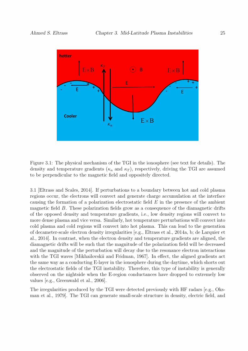
Ahmed S. Eltrass Chapter 3. Mid-Latitude Plasma Instabilities 25
Figure 3.1: The physical mechanism of the TGI in the ionosphere (see text for details). Thedensity and temperature gradients (κn and κT ), respectively, driving the TGI are assumedto be perpendicular to the magnetic field and oppositely directed.
3.1 [Eltrass and Scales, 2014]. If perturbations to a boundary between hot and cold plasmaregions occur, the electrons will convect and generate charge accumulation at the interfacecausing the formation of a polarization electrostatic field E in the presence of the ambientmagnetic field B. These polarization fields grow as a consequence of the diamagnetic driftsof the opposed density and temperature gradients, i.e., low density regions will convect tomore dense plasma and vice versa. Similarly, hot temperature perturbations will convect intocold plasma and cold regions will convect into hot plasma. This can lead to the generationof decameter-scale electron density irregularities [e.g., Eltrass et al., 2014a, b; de Larquier etal., 2014]. In contrast, when the electron density and temperature gradients are aligned, thediamagnetic drifts will be such that the magnitude of the polarization field will be decreasedand the magnitude of the perturbation will decay due to the resonance electron interactionswith the TGI waves [Mikhailovskii and Fridman, 1967]. In effect, the aligned gradients actthe same way as a conducting E-layer in the ionosphere during the daytime, which shorts outthe electrostatic fields of the TGI instability. Therefore, this type of instability is generallyobserved on the nightside when the E-region conductances have dropped to extremely lowvalues [e.g., Greenwald et al., 2006].
The irregularities produced by the TGI were detected previously with HF radars [e.g., Oks-man et al., 1979]. The TGI can generate small-scale structure in density, electric field, and
Ahmed S. Eltrass Chapter 3. Mid-Latitude Plasma Instabilities 26
electron temperature assuming that the electron density and temperature gradients are inopposite directions [e.g., Mikhailovskii, 1974; Hudson and Kelley, 1976]. Hudson and Kel-ley [1976] noted that the TGI might serve as an important energy source for the formationof the Stable Auroral Red (SAR) arc and the growth of irregularities at the equatorwardedge of the ionospheric plasma trough. Hudson and Kelley [1976] proposed that the de-velopment of the F-region TGI requires opposite temperature and density gradients. TheTGI can explain the observations of VLF and ELF waves on the plasmapause field lines bylow altitude spacecraft [e.g., Gurnett et al., 1969; Kelley, 1972]. Previous joint measure-ments by an oblique ionosonde located at Lindau, Germany and STARE VHF radar locatedin Hankasalmi, Finland have identified a band of irregularities equatorward of the STAREfield-of-view in the latitude range from L = 3.2-3.7 during the nighttime hours. Oksmanet al. [1979] suggested that these irregularities were produced by the TGI of Hudson andKelley [1976], but they did not provide measurements to support their suggestion. Sky im-ages collected by Nicolls et al. [2005] of a low density trough auroral red arc showed thatthe cross density/temperature gradient may be the reason for the small dynamic structureobserved on the poleward edge of this arc. Yizengaw and Moldwin [2005] showed that theequatorward wall of the mid-latitude ionospheric trough is magnetically conjugate to theplasmapause, while the opposed temperature and density gradients are the precise condi-tions for the generation of F-region TGI of Hudson and Kelley [1976]. Joint measurementsby the Millstone Hill Incoherent Scatter Radar (ISR) and the SuperDARN HF radar locatedat Wallops Island, Virginia detected decameter-scale irregularities with low drift velocities(< 100 m/s) in the quiet-time mid-latitude nightside ionosphere [Greenwald et al., 2006].Greenwald et al. [2006] showed that these irregularities were excited on the equatorwardwall of the mid-latitude ionospheric trough in a region of opposed density and temperaturegradients, and consequently they suggested that the TGI [i.e., Hudson and Kelley, 1976]could be a feasible mechanism for generating these irregularities.
3.1.1 TGI Fluid Model
The temperature gradient driven drift mode is obtained from the fluid theory by Kadomtsev[1965]. For a magnetic field in the z-direction, a perpendicular wave vector k⊥ in the y-direction, and gradients in the x-direction (see Figure 3.2), the wave frequency ω and growthrate γ for collisionless plasma are given by:
ω = k⊥
(kBTeqB0
)∇(ln(ne)) (3.1)
γ =√πω
(U
υte− 0.5
ωT
k∥υte
)(3.2)
where
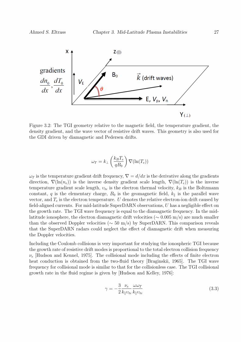
Ahmed S. Eltrass Chapter 3. Mid-Latitude Plasma Instabilities 27
Figure 3.2: The TGI geometry relative to the magnetic field, the temperature gradient, thedensity gradient, and the wave vector of resistive drift waves. This geometry is also used forthe GDI driven by diamagnetic and Pedersen drifts.
ωT = k⊥
(kBTeqB0
)∇(ln(Te))
ωT is the temperature gradient drift frequency, ∇ = d/dx is the derivative along the gradientsdirection, ∇(ln(ne)) is the inverse density gradient scale length, ∇(ln(Te)) is the inversetemperature gradient scale length, υte is the electron thermal velocity, kB is the Boltzmannconstant, q is the elementary charge, B0 is the geomagnetic field, k∥ is the parallel wavevector, and Te is the electron temperature. U denotes the relative electron-ion drift caused byfield-aligned currents. For mid-latitude SuperDARN observations, U has a negligible effect onthe growth rate. The TGI wave frequency is equal to the diamagnetic frequency. In the mid-latitude ionosphere, the electron diamagnetic drift velocities (∼ 0.005 m/s) are much smallerthan the observed Doppler velocities (∼ 50 m/s) by SuperDARN. This comparison revealsthat the SuperDARN radars could neglect the effect of diamagnetic drift when measuringthe Doppler velocities.
Including the Coulomb collisions is very important for studying the ionospheric TGI becausethe growth rate of resistive drift modes is proportional to the total electron collision frequencyνe [Hudson and Kennel, 1975]. The collisional mode including the effects of finite electronheat conduction is obtained from the two-fluid theory [Braginskii, 1965]. The TGI wavefrequency for collisional mode is similar to that for the collisionless case. The TGI collisionalgrowth rate in the fluid regime is given by [Hudson and Kelley, 1976]:
γ = −3
2
νek∥υte
ωωT
k∥υte(3.3)
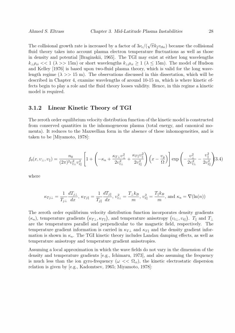
Ahmed S. Eltrass Chapter 3. Mid-Latitude Plasma Instabilities 28
The collisional growth rate is increased by a factor of 3νe/(√πk∥vthe) because the collisional
fluid theory takes into account plasma electron temperature fluctuations as well as thosein density and potential [Braginskii, 1965]. The TGI may exist at either long wavelengthsk⊥ρci << 1 (λ >> 15m) or short wavelengths k⊥ρci ≥ 1 (λ ≤ 15m). The model of Hudsonand Kelley [1976] is based upon two-fluid plasma theory, which is valid for the long wave-length regime (λ >> 15 m). The observations discussed in this dissertation, which will bedescribed in Chapter 4, examine wavelengths of around 10-15 m, which is where kinetic ef-fects begin to play a role and the fluid theory looses validity. Hence, in this regime a kineticmodel is required.
3.1.2 Linear Kinetic Theory of TGI
The zeroth order equilibrium velocity distribution function of the kinetic model is constructedfrom conserved quantities in the inhomogeneous plasma (total energy, and canonical mo-menta). It reduces to the Maxwellian form in the absence of these inhomogeneities, and istaken to be [Miyamoto, 1978]:
f0(x, υ⊥, υ∥) =n0
(2π)2υ2t⊥υ2t∥
[1 +
(−κn +
κT⊥υ2⊥
2υ2t⊥+κT∥υ
2∥
2υ2t∥
)(x− υy
Ω
)]exp
(− υ2⊥2υ2t⊥
−υ2∥2υ2t∥
)(3.4)
where
κTj⊥ =1
Tj⊥
dTj⊥dx
, κTj∥ =1
Tj∥
dTj∥dx
, υ2t⊥ =T⊥kBm
, υ2t∥ =T∥kBm
, and κn = ∇(ln(n))
The zeroth order equilibrium velocity distribution function incorporates density gradients(κn), temperature gradients
(κT⊥, κT∥
), and temperature anisotropy
(υt⊥, υt∥
). T∥ and T⊥
are the temperatures parallel and perpendicular to the magnetic field, respectively. Thetemperature gradient information is carried in κT⊥ and κT∥ and the density gradient infor-mation is shown in κn. The TGI kinetic theory includes Landau damping effects, as well astemperature anisotropy and temperature gradient anisotropies.
Assuming a local approximation in which the wave fields do not vary in the dimension of thedensity and temperature gradients [e.g., Ichimaru, 1973], and also assuming the frequencyis much less than the ion gyro-frequency (ω << Ωci), the kinetic electrostatic dispersionrelation is given by [e.g., Kadomtsev, 1965; Miyamoto, 1978]:

Ahmed S. Eltrass Chapter 3. Mid-Latitude Plasma Instabilities 29
k2⊥ + k2∥ +∑j
ω2pj
[mj
Tj⊥+ I0(bj)e
−bj
(mj
Tj∥− mj
Tj⊥
)+κTj∥ (ω + iνj)
2k2∥(Tj∥/mj
) k⊥Ωj
I0(bj) exp(−bj)
(1 + ζ0jZ(ζ0j)
)+ I0(bj) exp(−bj)ζ0jZ(ζ0j)
(mj
Tj∥+
k⊥(ω + iνj) Ωj(
−κj + (f0j − 1)κTj⊥ −κTj∥
2
))]/[1 +
iνjω + iνj
I0(bj) exp(−bj)ζ0jZ(ζ0j)]= 0 (3.5)
where
ζ0j =ω + iνj√
2k∥√Tj∥/mj
, f0(bj) = (1− bj) + bjI ′0(bj)
I0(bj), and bj = (k⊥ρj)
2
Here j = e, i stands for electron or ion. ωpj is the species plasma frequency, Ωj is the speciesgyro-frequency, ω is the wave frequency, νj is the species collision frequency, ρj is the speciesgyro-radius, mj is the species mass, κTj∥ is the zeroth-order parallel inverse temperaturegradient scale length, κTj⊥ is the zeroth-order perpendicular inverse temperature gradientscale length, I0(bj) is the zeroth order modified Bessel function of the first kind, Z(ζ0j) is theplasma dispersion function, and κj is the zeroth-order inverse density gradient scale length.k∥ and k⊥ are the perturbed wave numbers parallel and perpendicular to the magnetic field,respectively.
Neglecting the temperature anisotropy and the parallel temperature and density gradients,the simplified kinetic dispersion relation is given by [Eltrass et al., 2014a; Eltrass and Scales,2014]:
k2⊥ + k2∥ +∑j
ω2pj
[mj
Tj+ I0(bj) exp(−bj)ζ0jZ(ζ0j)
(mj
Tj+
k⊥(ω + iνj) Ωj
(−κnj + (f0j − 1)κTj))]/[
1 +iνj
ω + iνjI0(bj) exp(−bj)ζ0jZ(ζ0j)
]= 0 (3.6)
This TGI kinetic dispersion relation has been simplified to obtain approximate analyticalexpressions for the TGI wave frequency and growth rate [Appendix A] that can be seen to beextensions of past work using fluid theory appropriate for k⊥ρci << 1 (λ >> 15m) [Hudsonand Kelley, 1976]. Neglecting the electron gyro-radius and temperature anisotropy, the TGIwave frequency ω and growth rate γ are given by [e.g., Mikhailovskii, 1974; Dimits and Lee,1991]:

Ahmed S. Eltrass Chapter 3. Mid-Latitude Plasma Instabilities 30
0 0.5 1 1.5 20
0.5
1
1.5x 10
−6 (a) Hudson & Kelley [1976]
kρci
γ/Ω
ci
νe=8.2 Hz
νe=20 Hz
νe=30 Hz
νe=50 Hz
0 0.5 1 1.5 20
0.5
1
1.5x 10
−6(b) Kinetic Dispersion Relation
kρci
γ/Ω
ci
ν
e=8.2 Hz
νe=20 Hz
νe=30 Hz
νe=50 Hz
Figure 3.3: The TGI growth rates of (a) fluid theory of Hudson and Kelley [1976] (equation3.3) and (b) kinetic theory (equation 3.5) for four different electron collision frequencies ataltitude 1050 km. The parameters used for computations are listed in Table 3.1.
ω ≈ ω∗Γ0(bi)
Γ0(bi)− (1 + τ)(3.7)
γ ≈ 2νeω∗ωTΓ0(bi)
k2∥υ2te [Γ0(bi)− (1 + τ)]2
(3.8)
where
ω∗ = k⊥
(kBTeqB0
)κne, ωT = k⊥
(kBTeqB0
)κTe, Γ0(bi) = I0(bi) exp(−bi), and τ = Te/Ti
ωT is the temperature gradient drift frequency, ω∗ is the diamagnetic frequency, υte is theelectron thermal velocity, kB is the Boltzmann constant, Ti is the ion temperature, andTe is the electron temperature. It should be noted that the growth rate due to TGI isproportional to the product of the diamagnetic frequency and the temperature gradient driftfrequency, γ ∝ ωnωT . The results in equations (3.7) and (3.8) reduce to that of Hudsonand Kelley [1976] in the long wavelength regime k⊥ρci << 1, which corresponds to λ >> 15m. A rough approximation for the wave number for maximum growth can be determined
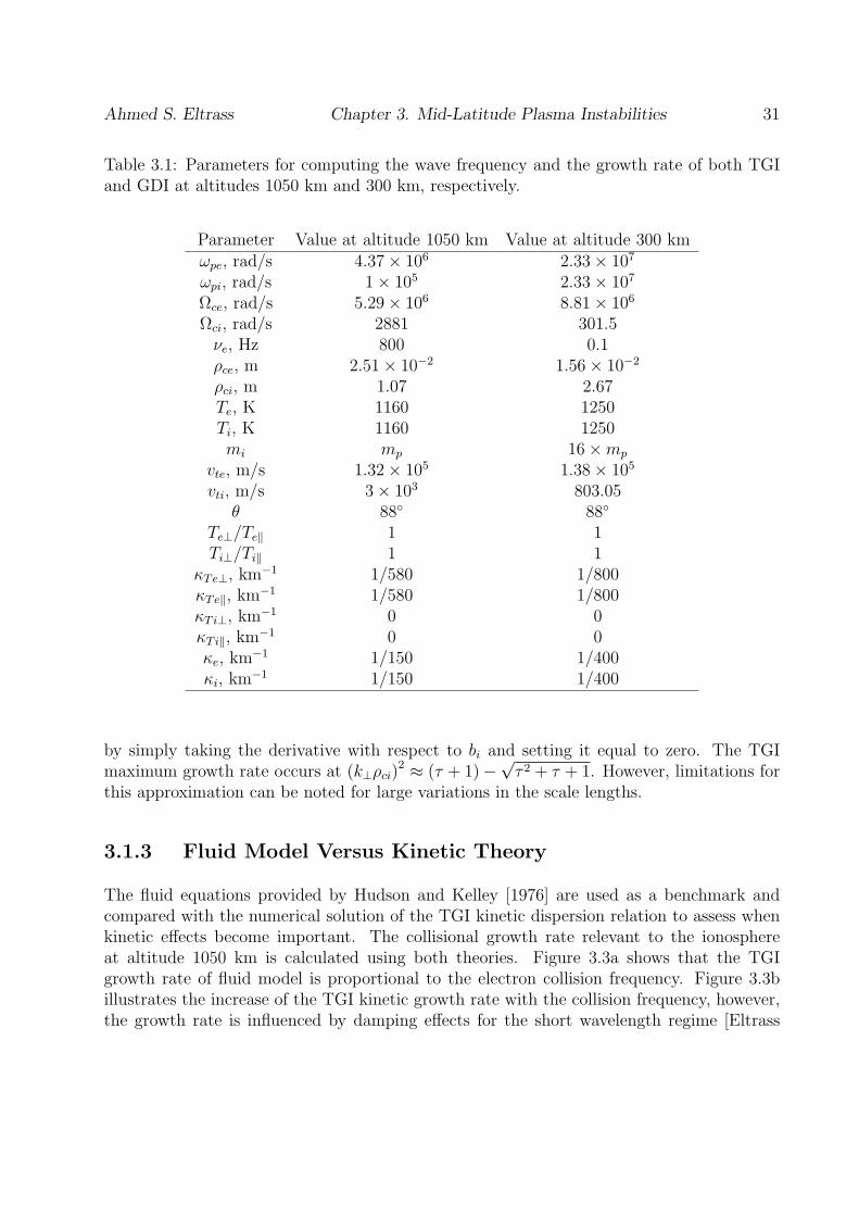
Ahmed S. Eltrass Chapter 3. Mid-Latitude Plasma Instabilities 31
Table 3.1: Parameters for computing the wave frequency and the growth rate of both TGIand GDI at altitudes 1050 km and 300 km, respectively.
Parameter Value at altitude 1050 km Value at altitude 300 kmωpe, rad/s 4.37× 10⁶ 2.33× 10⁷
ωpi, rad/s 1× 10⁵ 2.33× 10⁷
Ωce, rad/s 5.29× 10⁶ 8.81× 10⁶
Ωci, rad/s 2881 301.5νe, Hz 800 0.1ρce, m 2.51× 10⁻² 1.56× 10⁻²
ρci, m 1.07 2.67Te, K 1160 1250Ti, K 1160 1250mi mp 16×mp
vte, m/s 1.32× 10⁵ 1.38× 10⁵
vti, m/s 3× 10³ 803.05θ 88 88
Te⊥/Te∥ 1 1Ti⊥/Ti∥ 1 1
κTe⊥, km−1 1/580 1/800
κTe∥, km−1 1/580 1/800
κTi⊥, km−1 0 0
κTi∥, km−1 0 0
κe, km−1 1/150 1/400
κi, km−1 1/150 1/400
by simply taking the derivative with respect to bi and setting it equal to zero. The TGImaximum growth rate occurs at (k⊥ρci)
2 ≈ (τ + 1)−√τ 2 + τ + 1. However, limitations for
this approximation can be noted for large variations in the scale lengths.
3.1.3 Fluid Model Versus Kinetic Theory
The fluid equations provided by Hudson and Kelley [1976] are used as a benchmark andcompared with the numerical solution of the TGI kinetic dispersion relation to assess whenkinetic effects become important. The collisional growth rate relevant to the ionosphereat altitude 1050 km is calculated using both theories. Figure 3.3a shows that the TGIgrowth rate of fluid model is proportional to the electron collision frequency. Figure 3.3billustrates the increase of the TGI kinetic growth rate with the collision frequency, however,the growth rate is influenced by damping effects for the short wavelength regime [Eltrass
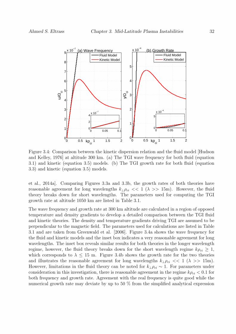
Ahmed S. Eltrass Chapter 3. Mid-Latitude Plasma Instabilities 32
0 0.5 1 1.5 20
1
2
3
4
5
6
7
8
9x 10
−7
kρci
ω/Ω
ci
(a) Wave Frequency
Fluid Model Kinetic Model
0 0.5 1 1.5 20
1
2
3
4
5
x 10−4
(b) Growth Rate
kρci
γ/Ω
ci
Fluid Model Kinetic Model
0 0.05 0.10
5
x 10−4
0 0.05 0.10
2
4x 10
−7
Figure 3.4: Comparison between the kinetic dispersion relation and the fluid model [Hudsonand Kelley, 1976] at altitude 300 km. (a) The TGI wave frequency for both fluid (equation3.1) and kinetic (equation 3.5) models. (b) The TGI growth rate for both fluid (equation3.3) and kinetic (equation 3.5) models.
et al., 2014a]. Comparing Figures 3.3a and 3.3b, the growth rates of both theories havereasonable agreement for long wavelengths k⊥ρci << 1 (λ >> 15m). However, the fluidtheory breaks down for short wavelengths. The parameters used for computing the TGIgrowth rate at altitude 1050 km are listed in Table 3.1.
The wave frequency and growth rate at 300 km altitude are calculated in a region of opposedtemperature and density gradients to develop a detailed comparison between the TGI fluidand kinetic theories. The density and temperature gradients driving TGI are assumed to beperpendicular to the magnetic field. The parameters used for calculations are listed in Table3.1 and are taken from Greenwald et al. [2006]. Figure 3.4a shows the wave frequency forthe fluid and kinetic models and the inset box indicates a very reasonable agreement for longwavelengths. The inset box reveals similar results for both theories in the longer wavelengthregime, however, the fluid theory breaks down for the short wavelength regime kρci ≥ 1,which corresponds to λ ≤ 15 m. Figure 3.4b shows the growth rate for the two theoriesand illustrates the reasonable agreement for long wavelengths k⊥ρci << 1 (λ >> 15m).However, limitations in the fluid theory can be noted for k⊥ρci ∼ 1. For parameters underconsideration in this investigation, there is reasonable agreement in the regime kρci < 0.1 forboth frequency and growth rate. Agreement with the real frequency is quite good while thenumerical growth rate may deviate by up to 50 % from the simplified analytical expression
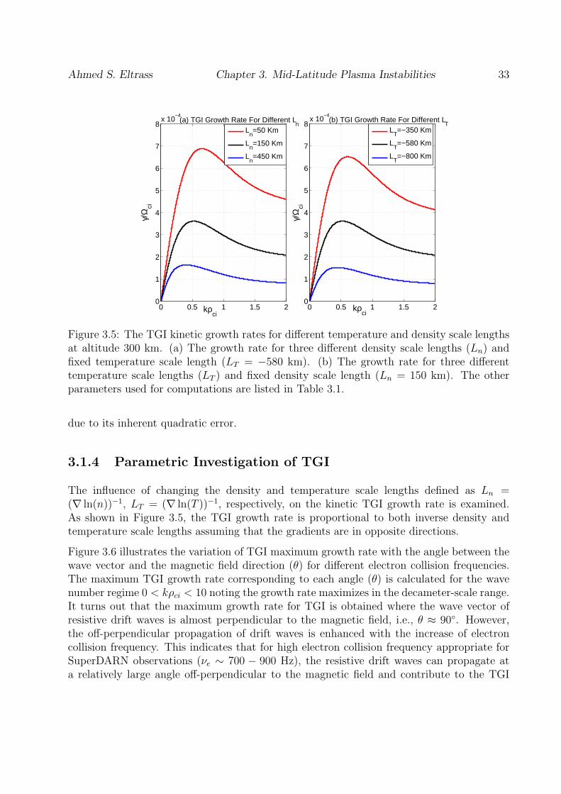
Ahmed S. Eltrass Chapter 3. Mid-Latitude Plasma Instabilities 33
0 0.5 1 1.5 20
1
2
3
4
5
6
7
8x 10
−4
kρci
γ/Ω
ci
(a) TGI Growth Rate For Different Ln
L
n=50 Km
Ln=150 Km
Ln=450 Km
0 0.5 1 1.5 20
1
2
3
4
5
6
7
8x 10
−4
kρci
γ/Ω
ci
(b) TGI Growth Rate For Different LT
L
T=−350 Km
LT=−580 Km
LT=−800 Km
Figure 3.5: The TGI kinetic growth rates for different temperature and density scale lengthsat altitude 300 km. (a) The growth rate for three different density scale lengths (Ln) andfixed temperature scale length (LT = −580 km). (b) The growth rate for three differenttemperature scale lengths (LT ) and fixed density scale length (Ln = 150 km). The otherparameters used for computations are listed in Table 3.1.
due to its inherent quadratic error.
3.1.4 Parametric Investigation of TGI
The influence of changing the density and temperature scale lengths defined as Ln =(∇ ln(n))−1, LT = (∇ ln(T ))−1, respectively, on the kinetic TGI growth rate is examined.As shown in Figure 3.5, the TGI growth rate is proportional to both inverse density andtemperature scale lengths assuming that the gradients are in opposite directions.
Figure 3.6 illustrates the variation of TGI maximum growth rate with the angle between thewave vector and the magnetic field direction (θ) for different electron collision frequencies.The maximum TGI growth rate corresponding to each angle (θ) is calculated for the wavenumber regime 0 < kρci < 10 noting the growth rate maximizes in the decameter-scale range.It turns out that the maximum growth rate for TGI is obtained where the wave vector ofresistive drift waves is almost perpendicular to the magnetic field, i.e., θ ≈ 90. However,the off-perpendicular propagation of drift waves is enhanced with the increase of electroncollision frequency. This indicates that for high electron collision frequency appropriate forSuperDARN observations (νe ∼ 700 − 900 Hz), the resistive drift waves can propagate ata relatively large angle off-perpendicular to the magnetic field and contribute to the TGI
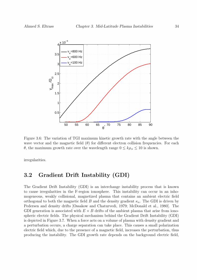
Ahmed S. Eltrass Chapter 3. Mid-Latitude Plasma Instabilities 34
50 55 60 65 70 75 80 85 90
0.5
1
1.5
2
2.5
3
3.5
4x 10
−4
θ°
γ max
/Ωci
νe=800 Hz
νe=600 Hz
νe=100 Hz
Figure 3.6: The variation of TGI maximum kinetic growth rate with the angle between thewave vector and the magnetic field (θ) for different electron collision frequencies. For eachθ, the maximum growth rate over the wavelength range 0 ≤ kρci ≤ 10 is shown.
irregularities.
3.2 Gradient Drift Instability (GDI)
The Gradient Drift Instability (GDI) is an interchange instability process that is knownto cause irregularities in the F-region ionosphere. This instability can occur in an inho-mogeneous, weakly collisional, magnetized plasma that contains an ambient electric fieldorthogonal to both the magnetic field B and the density gradient κn. The GDI is driven byPedersen and density drifts [Ossakow and Chaturvedi, 1979; McDonald et al., 1980]. TheGDI generation is associated with E ×B drifts of the ambient plasma that arise from iono-spheric electric fields. The physical mechanism behind the Gradient Drift Instability (GDI)is depicted in Figure 3.7. When a force acts on a volume of plasma with density gradient anda perturbation occurs, a charge separation can take place. This causes a small polarizationelectric field which, due to the presence of a magnetic field, increases the perturbation, thusproducing the instability. The GDI growth rate depends on the background electric field,
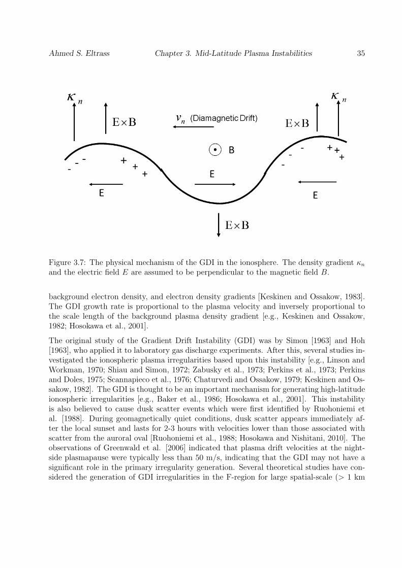
Ahmed S. Eltrass Chapter 3. Mid-Latitude Plasma Instabilities 35
Figure 3.7: The physical mechanism of the GDI in the ionosphere. The density gradient κnand the electric field E are assumed to be perpendicular to the magnetic field B.
background electron density, and electron density gradients [Keskinen and Ossakow, 1983].The GDI growth rate is proportional to the plasma velocity and inversely proportional tothe scale length of the background plasma density gradient [e.g., Keskinen and Ossakow,1982; Hosokawa et al., 2001].
The original study of the Gradient Drift Instability (GDI) was by Simon [1963] and Hoh[1963], who applied it to laboratory gas discharge experiments. After this, several studies in-vestigated the ionospheric plasma irregularities based upon this instability [e.g., Linson andWorkman, 1970; Shiau and Simon, 1972; Zabusky et al., 1973; Perkins et al., 1973; Perkinsand Doles, 1975; Scannapieco et al., 1976; Chaturvedi and Ossakow, 1979; Keskinen and Os-sakow, 1982]. The GDI is thought to be an important mechanism for generating high-latitudeionospheric irregularities [e.g., Baker et al., 1986; Hosokawa et al., 2001]. This instabilityis also believed to cause dusk scatter events which were first identified by Ruohoniemi etal. [1988]. During geomagnetically quiet conditions, dusk scatter appears immediately af-ter the local sunset and lasts for 2-3 hours with velocities lower than those associated withscatter from the auroral oval [Ruohoniemi et al., 1988; Hosokawa and Nishitani, 2010]. Theobservations of Greenwald et al. [2006] indicated that plasma drift velocities at the night-side plasmapause were typically less than 50 m/s, indicating that the GDI may not have asignificant role in the primary irregularity generation. Several theoretical studies have con-sidered the generation of GDI irregularities in the F-region for large spatial-scale (> 1 km
Ahmed S. Eltrass Chapter 3. Mid-Latitude Plasma Instabilities 36
in wavelength) [Kelley et al., 1982; Keskinen and Ossakow, 1983; Tsunoda, 1988]. Despitea good level of theoretical understanding of large-scale GDI irregularities, more studies arerequired at small spatial scales [Kelley, 2009]. Important effects to be considered in furtherdetail include nonlinear cascading and the impact of E-region conductance.
3.2.1 Fluid Theory of GDI
Ossakow et al. [1978] investigated the GDI in the fluid regime for F-region plasma cloudsand found that there is a further difference of the instability according to the altitude range.Based on the relative importance of inertia versus ion-neutral collisions in the GDI, we canconsider two separate regimes as following:
• Low altitude limit (∼ 200− 300 km): in this collisional regime, the ion inertial effects canbe neglected. The GDI wave frequency ω and growth rate γ for this regime are given by:
ω = k⊥υni νe >> 4κnυE (3.9)
γ ≈ κnυE νi >> 4κnυE (3.10)
where υE = E/B is the E × B drift velocity, υni = κnυ2ti/Ωci is the ion diamagnetic drift
velocity, κn is the inverse density gradient scale length, νi is the ion collision frequency, andΩci is the ion gyro-frequency. The form of low altitude limit represents the usual E × BGradient Drift Instability (GDI) for plasma clouds in the ionosphere [Linson and Workman,1970].
• High altitude limit (∼ 450 km): the ion inertial effects at high altitudes become more im-portant because the ion-neutral collision frequency decreases due to the reduction in neutraldensity. The GDI growth rate in this case is given by:
γ = (κnυEνi)1/2 νi << 4κnυE (3.11)
The model of Ossakow et al. [1978] is appropriate for investigating the GDI for long wave-lengths in the collisional regime of the F-region ionosphere. However, as described by Garyand Cole [1983], a kinetic model is more accurate in the short wavelength regime whenk⊥ρci ≈ 1.
3.2.2 Linear Kinetic Theory of GDI
The GDI generation is assumed to be due to two sources of free energy: the density gradientin the x-direction and the electric field in the y-direction perpendicular to both density
Ahmed S. Eltrass Chapter 3. Mid-Latitude Plasma Instabilities 37
gradient and magnetic field. As shown in Figure 3.2, the geometry used in the analysis ofthe GDI driven by Pedersen υp and diamagnetic drift velocities υn is similar to that of TGI.The GDI kinetic dispersion relation based on the Gary and Cole [1983] model is used toallow the study of GDI for short wavelengths (decameter-scale waves).
The zeroth order equilibrium velocity distribution function [Gary and Cole, 1983] is takento be:
f0(x, υ) =n0
(2πυ2t )3/2
[1 + κn
(x+
υyΩ
− νυxΩ2
)+υEυt
(υxυt
+ νυyΩυt
)]exp
(− υ2
2υ2t
)(3.12)
The zeroth order equilibrium velocity distribution function incorporates collisional effects(ν), density gradients (κn), and E ×B drift velocity (υE = E/B).
Assuming local approximation and that the frequency is much less than the ion gyro-frequency, the GDI kinetic dispersion relation including finite ion gyro-radius effects is givenby [Gary and Cole, 1983]:
1 +∑j
k2Dj
k2
[1 +
(ω − kυnj − kυpj)Aj(k, ω)−Nj(k, ω)
1 + νjAj(k, ω)− i (υpj/υtj)Rxj(k, ω)
]= 0 (3.13)
where Aj(k, ω) and Rj(k, ω) are expressed as [Appendix B]:
Aj(k, ω) =1√
2k∥υtj
∞∑n=−∞
Γn(bj)Z(ζjn) =1√
2k∥υtj
8∑m=1
rmk∥ρjbjY 2
(R(Y, bj) +
Y
bj
)(3.14)
Rxj(k, ω) =ik⊥υtj√2k∥υtj
∞∑n=−∞
Z(ζjn) [Γn(bj)− Γ′n(bj)]
=ik⊥υtj√2k∥υtj
[1√
2k∥υtj
8∑m=1
rmk∥ρjbjY 2
(R(Y, bj) +
Y
bj
)−
8∑m=1
rmk∥ρjY 2
R′(Y, bj)
](3.15)
Ryj(k, ω) =Ω2
j√2k∥k⊥υ2tj
∞∑n=−∞
nΓn(bj)Z(ζjn) =1√
2k∥υtj
Ω2j
k⊥υtj
8∑m=1
rmk∥ρjbjY
R(Y, bj) (3.16)
and
Ahmed S. Eltrass Chapter 3. Mid-Latitude Plasma Instabilities 38
N(k, ω) =ω(υnj + υpj)
Ωj
Ryj(k, ω) +ωνjυnjΩ2
jυtjRxj(k, ω) (3.17)
This version of the GDI dispersion relation, with all |m| ≥ 1 terms in the Bessel sums ofAj(k, ω) and Rj(k, ω), is used to investigate the variation of GDI maximum growth rate withthe angle between the wave vector and the magnetic field direction (θ). Further numericalcalculations have shown that it is a reasonably good approximation to ignore all |m| ≥ 1terms in the Bessel sums of Aj(k, ω) and Rj(k, ω). Also, the calculations show that themaximum GDI growth rate is obtained at k∥ = 0 (i.e., θ ≈ 90) for all parameters underconsideration in this investigation. Neglecting the parallel wave vector (k∥ = 0), i.e., θ ≈ 90,the Bessel sums of Aj(k, ω) and Rj(k, ω) are given by:
Aj(k, ω) = −exp(−bj)ω + iνj
I0(bj) (3.18)
Rxj(k, ω) = − ik⊥υtjω + iνj
exp(−bj) [I0(bj)− I ′0(bj)] (3.19)
and
Ryj(k, ω) = − Ωj
k⊥υtj[1− exp(−bj)I0(bj)] (3.20)
The diamagnetic drift velocity of the jth species is υnj = κnυ2tj/Ωj and the Pedersen drift
velocity is υpj = νjυE/Ωj.
Since frequencies much less than the ion gyro-frequency are considered, ω << Ωci, theinfinite Bessel function sums for Aj(k, ω) and Rj(k, ω) are neglected [Gary and Cole, 1983]and only the zeroth order Bessel function is retained. This treatment is used to study theproperties of instabilities for short wavelengths, however, the well known results for the longwavelength GDI could be also derived from this kinetic model. The short wavelength regimewould typically be expected to be excited with electric fields, E, larger than for the longwavelength version. However, the E×B drift velocity is still much less than the ion thermalvelocity.
Figures 3.8a and 3.8b show the wave frequency and the growth rate, respectively, as a functionof wave number in the limit of collisionless electrons and collisional ions. The parametersused for computations are for Gary and Cole [1983]. It can be noted that the GDI growth canpersist to very short wavelength (kρci >> 1). For υpi > 0.3υni, the kinetic GDI dispersionrelation yields maximum growth rate slightly larger than that of the fluid theory [Gary andThomsen, 1982]. The calculations of Gary and Cole [1983] established the conditions on theelectron and ion collision frequencies that allow the GDI to grow at kρci ≥ 1. If the E × B
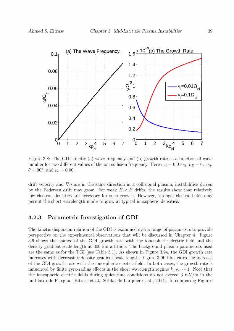
Ahmed S. Eltrass Chapter 3. Mid-Latitude Plasma Instabilities 39
0 1 2 3 4 5 6 70
0.02
0.04
0.06
0.08
0.1
kρci
ω/Ω
ci (a) The Wave Frequency
0 1 2 3 4 5 6 70
0.2
0.4
0.6
0.8
1
1.2
1.4
1.6x 10
−3
kρci
γ/Ω
ci
(b) The Growth Rate
νi=0.01Ω
ci
νi=0.1Ω
ci
Figure 3.8: The GDI kinetic (a) wave frequency and (b) growth rate as a function of wavenumber for two different values of the ion collision frequency. Here υni = 0.01υti, υE = 0.1υti,θ = 90, and νe = 0.00.
drift velocity and ∇n are in the same direction in a collisional plasma, instabilities drivenby the Pedersen drift may grow. For weak E × B drifts, the results show that relativelylow electron densities are necessary for such growth. However, stronger electric fields maypermit the short wavelength mode to grow at typical ionospheric densities.
3.2.3 Parametric Investigation of GDI
The kinetic dispersion relation of the GDI is examined over a range of parameters to provideperspective on the experimental observations that will be discussed in Chapter 4. Figure3.9 shows the change of the GDI growth rate with the ionospheric electric field and thedensity gradient scale length at 300 km altitude. The background plasma parameters usedare the same as for the TGI (see Table 3.1). As shown in Figure 3.9a, the GDI growth rateincreases with decreasing density gradient scale length. Figure 3.9b illustrates the increaseof the GDI growth rate with the ionospheric electric field. In both cases, the growth rate isinfluenced by finite gyro-radius effects in the short wavelength regime k⊥ρci ∼ 1. Note thatthe ionospheric electric fields during quiet-time conditions do not exceed 3 mV/m in themid-latitude F-region [Eltrass et al., 2014a; de Larquier et al., 2014]. In comparing Figures
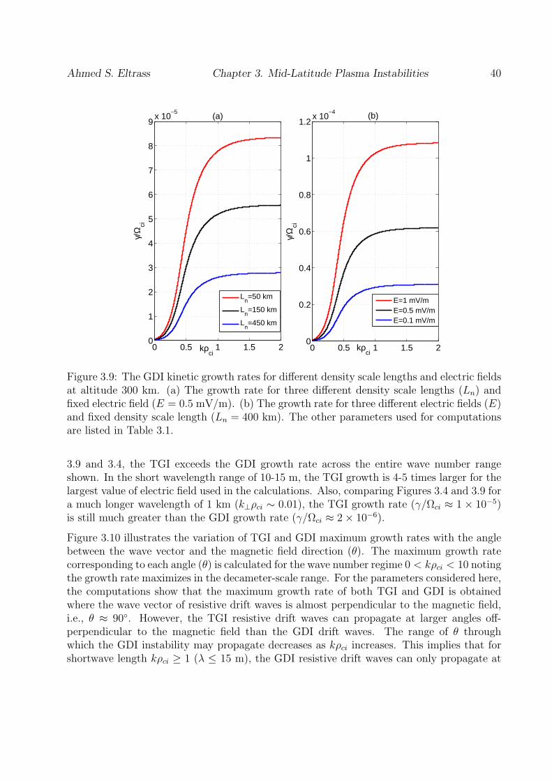
Ahmed S. Eltrass Chapter 3. Mid-Latitude Plasma Instabilities 40
0 0.5 1 1.5 20
1
2
3
4
5
6
7
8
9x 10
−5
kρci
γ/Ω
ci
(a)
Ln=50 km
Ln=150 km
Ln=450 km
0 0.5 1 1.5 20
0.2
0.4
0.6
0.8
1
1.2x 10
−4
kρci
γ/Ω
ci
(b)
E=1 mV/mE=0.5 mV/mE=0.1 mV/m
Figure 3.9: The GDI kinetic growth rates for different density scale lengths and electric fieldsat altitude 300 km. (a) The growth rate for three different density scale lengths (Ln) andfixed electric field (E = 0.5 mV/m). (b) The growth rate for three different electric fields (E)and fixed density scale length (Ln = 400 km). The other parameters used for computationsare listed in Table 3.1.
3.9 and 3.4, the TGI exceeds the GDI growth rate across the entire wave number rangeshown. In the short wavelength range of 10-15 m, the TGI growth is 4-5 times larger for thelargest value of electric field used in the calculations. Also, comparing Figures 3.4 and 3.9 fora much longer wavelength of 1 km (k⊥ρci ∼ 0.01), the TGI growth rate (γ/Ωci ≈ 1× 10⁻⁵)is still much greater than the GDI growth rate (γ/Ωci ≈ 2× 10⁻⁶).
Figure 3.10 illustrates the variation of TGI and GDI maximum growth rates with the anglebetween the wave vector and the magnetic field direction (θ). The maximum growth ratecorresponding to each angle (θ) is calculated for the wave number regime 0 < kρci < 10 notingthe growth rate maximizes in the decameter-scale range. For the parameters considered here,the computations show that the maximum growth rate of both TGI and GDI is obtainedwhere the wave vector of resistive drift waves is almost perpendicular to the magnetic field,i.e., θ ≈ 90. However, the TGI resistive drift waves can propagate at larger angles off-perpendicular to the magnetic field than the GDI drift waves. The range of θ throughwhich the GDI instability may propagate decreases as kρci increases. This implies that forshortwave length kρci ≥ 1 (λ ≤ 15 m), the GDI resistive drift waves can only propagate at
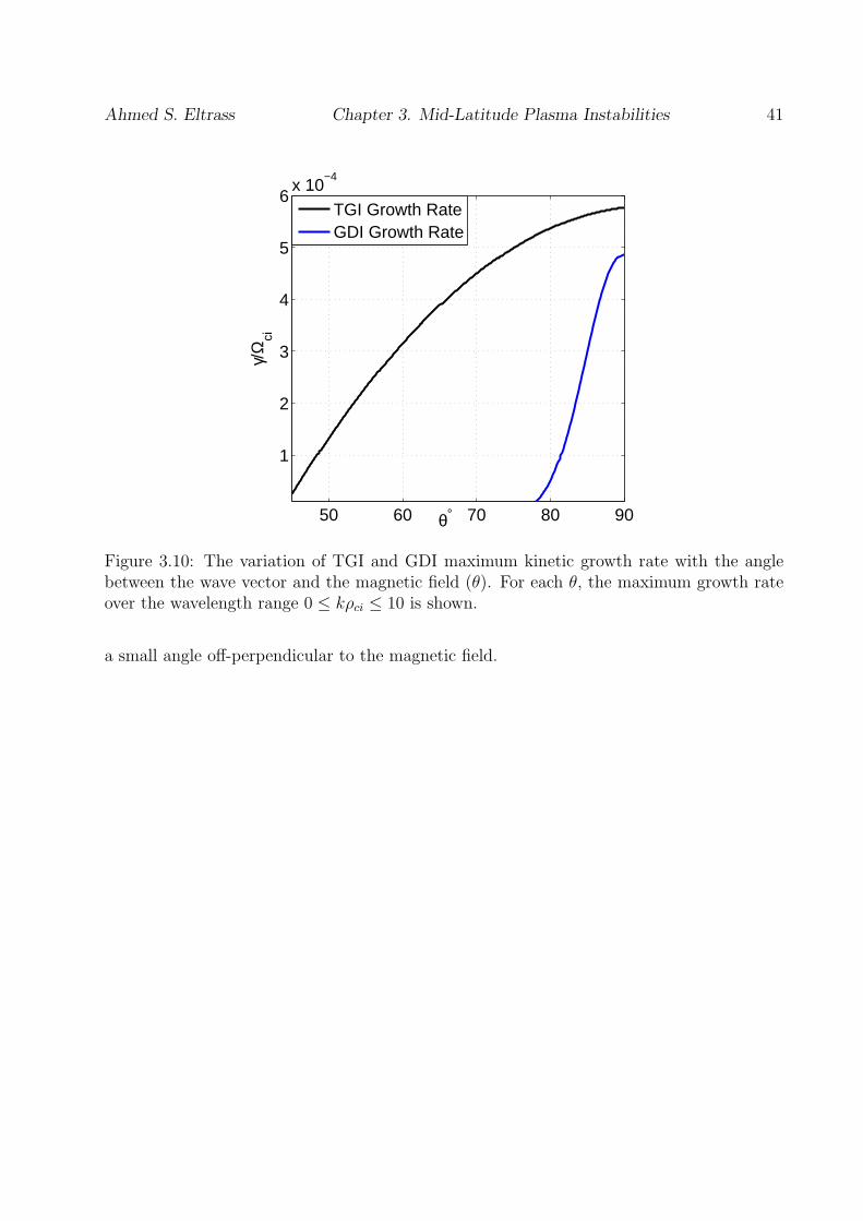
Ahmed S. Eltrass Chapter 3. Mid-Latitude Plasma Instabilities 41
50 60 70 80 90
1
2
3
4
5
6x 10
−4
θ°
γ/Ω
ci
TGI Growth RateGDI Growth Rate
Figure 3.10: The variation of TGI and GDI maximum kinetic growth rate with the anglebetween the wave vector and the magnetic field (θ). For each θ, the maximum growth rateover the wavelength range 0 ≤ kρci ≤ 10 is shown.
a small angle off-perpendicular to the magnetic field.
Chapter 4
Experimental Radar Observations ofMid-Latitude Irregularities
4.1 Quiet-Time Ionospheric Irregularities
During geomagnetically quiet conditions (Kp ≤ 2), the mid-latitude ionosphere (30 to 60
geomagnetic latitude) is a quiescent plasma but still populated by plasma density irregular-ities generated by both plasma and neutral processes. The mid-latitude SuperDARN radarsfrequently observe quiet-time decameter-scale ionospheric irregularities that have been pro-posed to be responsible for the observed low-velocity Sub-Auroral Ionospheric Scatter (SAIS)[e.g., Greenwald et al., 2006; Ribeiro et al., 2012; Kane et al., 2012]. Greenwald et al. [2006]observed a new type of backscatter from mid-latitude ionospheric irregularities on the night-side during quiescent conditions. Based on the coordination between the Millstone HillIncoherent Scatter Radar (ISR) and the SuperDARN HF radar located at Wallops Island,Virginia, Greenwald et al. [2006] reported recurring quiet-time decameter-scale irregularitieswith low drift velocities (< 100 m/s) in the nightside sub-auroral ionosphere. They showedthat these irregularities are excited on the equatorward wall of the mid-latitude ionospherictrough, where opposed temperature and density gradients are presented. Using 3 years ofdata from the second mid-latitude SuperDARN HF radar located at Blackstone, Virginia,Ribeiro et al. [2012] showed that such irregularities are confined to local night and remainequatorward of both the auroral region and the ionospheric projection of the plasmapause.One question which remains unanswered is what type of plasma instability mechanism isresponsible for the growth of these decameter-scale ionospheric irregularities. In order tounderstand the physical mechanisms responsible for the formation of these irregularities, anew approach for the analysis of TGI and GDI growth rates is developed. By re-derivingthe electron density and temperature gradients in the plane perpendicular to B, a detailedcomparison of TGI and GDI is made for the observations of Greenwald et al. [2006] by thedevelopment of the kinetic growth rate time series for both TGI and GDI [Eltrass et al.,
42
Ahmed S. Eltrass Chapter 4. Experimental Radar Observations of Mid-Latitude Irregularities 43
2014a, b].
4.1.1 SuperDARN Observations
On the night of 22-23 February 2006, the Wallops SuperDARN radar and Millstone Hill ISRwere running co-located observations of sub-auroral ionospheric irregularities [Greenwald etal., 2006]. The Wallops SuperDARN radar (37.93 N, −75.47 E) was operating in a standard16-position azimuth-scanning mode with a dwell time of 3 seconds in each azimuth directionand a scan repetition time of 60 seconds. The data are sampled at 110 range gates extendingfrom 180 km to 5130 km with a slant-range gate of 45 km. Each slant-range gate stores ameasure for the power, line-of-sight Doppler velocity, and spectral width of the backscatter.Due to the large Doppler variability associated with the nominally low-velocity irregularities,short dwell times were used. The geomagnetic coordinates of the backscatter positions arecalculated using the Altitude Adjusted Corrected GeoMagnetic (AACGM) coordinate system[Baker and Wing, 1989]. The altitude and elevation are determined as a function of the slant-range utilizing a simple linear model [Chisham et al., 2008]. The observations during thisevent were predominantly from F-region decameter-scale ionospheric irregularities extendingfrom 500-1400 km in range from Wallops radar, relevant to latitudes from 52 to 59.
Figure 4.1 shows the observation geometry, where the Millstone Hill ISR pointing directionis aligned with beam 9 of the Wallops SuperDARN radar [Eltrass et al., 2014b]. We alsodisplay the backscatter distribution due to ionospheric density irregularities between 00:00and 05:00 UT, showing that Millstone Hill ISR is ideally located below the backscatterobserved at Wallops SuperDARN radar. Beam 3 is directed about 11.5 to the east of thegeographic meridian, while beam 9 passes overhead of Millstone Hill. Figure 4.2 shows thebackscatter power and line-of-sight Doppler velocity observed by the Wallops SuperDARNradar along beam 9 (top two panels) and beam 3 (bottom two panels) on the night ofFebruary 22-23, 2006. The first and third panels show the relative backscattered power indB, while other panels show the line-of-sight Doppler velocity in m/s. The observationsduring this event show both types of backscatter, ground and ionospheric scatter. First,the scatter from higher magnetic latitudes over the time interval 22:00 to 00:00 UT (beforesunset) is ground backscatter, which occurs after an oblique reflection of the radar signalby the ionosphere when the ionospheric plasma frequency is sufficiently high. The groundscatter is observed with a small but predominantly negative Doppler velocity due to theapparent upward motion of the ionosphere around sunset when photoionization drops. At23:10 UT, the operating frequency of the radar is lowered from 14.5 MHz to 11.0 MHz toaccommodate for the drop in plasma critical frequency during the night [e.g., Davies, 1990].This causes the discontinuity shown in Figure 4.2. After sunset (from 00:10 to 05:00 UT),the radar begins to observe low-velocity Sub-Auroral Ionospheric Scatter (SAIS) [Greenwaldet al., 2006; Ribeiro et al. 2012] with a small but predominantly positive (i.e., westward)Doppler velocity over latitudes from 56 to 59 on most of the Wallops radar beams. Theionospheric irregularities responsible for the observed scatter are seen in the top-side F-
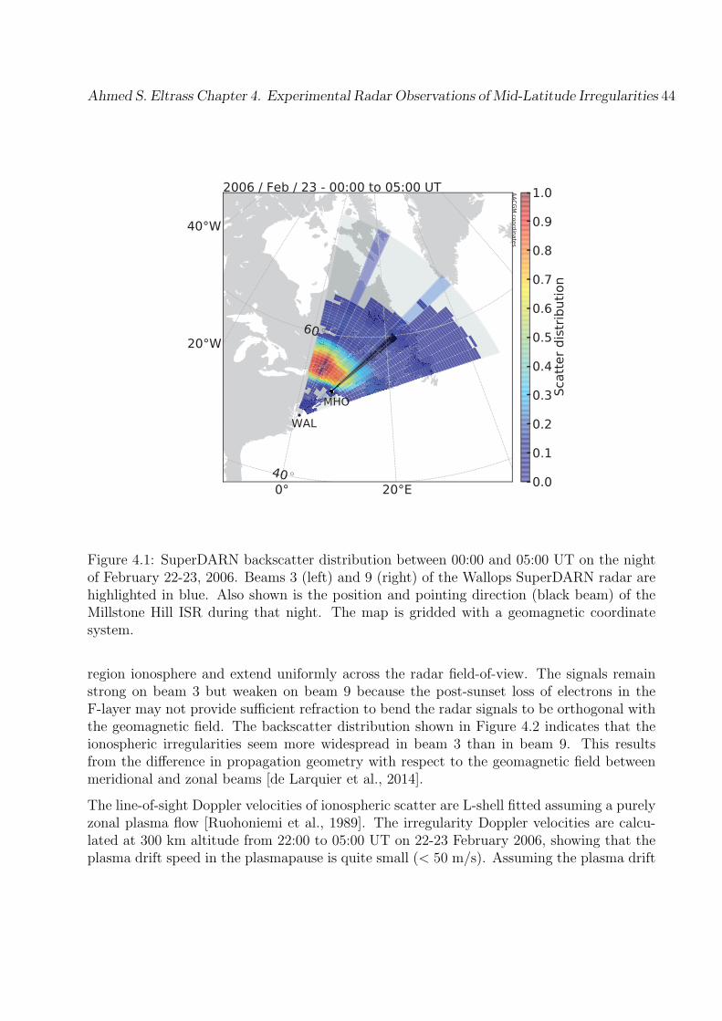
Ahmed S. Eltrass Chapter 4. Experimental Radar Observations of Mid-Latitude Irregularities 44
Figure 4.1: SuperDARN backscatter distribution between 00:00 and 05:00 UT on the nightof February 22-23, 2006. Beams 3 (left) and 9 (right) of the Wallops SuperDARN radar arehighlighted in blue. Also shown is the position and pointing direction (black beam) of theMillstone Hill ISR during that night. The map is gridded with a geomagnetic coordinatesystem.
region ionosphere and extend uniformly across the radar field-of-view. The signals remainstrong on beam 3 but weaken on beam 9 because the post-sunset loss of electrons in theF-layer may not provide sufficient refraction to bend the radar signals to be orthogonal withthe geomagnetic field. The backscatter distribution shown in Figure 4.2 indicates that theionospheric irregularities seem more widespread in beam 3 than in beam 9. This resultsfrom the difference in propagation geometry with respect to the geomagnetic field betweenmeridional and zonal beams [de Larquier et al., 2014].
The line-of-sight Doppler velocities of ionospheric scatter are L-shell fitted assuming a purelyzonal plasma flow [Ruohoniemi et al., 1989]. The irregularity Doppler velocities are calcu-lated at 300 km altitude from 22:00 to 05:00 UT on 22-23 February 2006, showing that theplasma drift speed in the plasmapause is quite small (< 50 m/s). Assuming the plasma drift

Ahmed S. Eltrass Chapter 4. Experimental Radar Observations of Mid-Latitude Irregularities 45
TGI driven irregularities
Figure 4.2: Backscatter observed by the Wallops SuperDARN radar on 22-23 February 2006from 22:00 to 05:00 UT in beam 9 (top 2 panels) and beam 3 (bottom 2 panels). Thebackscatter power and Doppler velocities are shown for each beam.
is mainly driven by E×B, the F-region electric field is calculated as E = υB, where E is theelectric field and B is the geomagnetic field. The observed Doppler velocities in the F-regionduring this event yield electric fields less than 3 mV/m. The calculated electric fields areused to compute the GDI growth rates.
4.1.2 Millstone Hill ISR Observations
In order to understand the physical mechanisms responsible for the observed irregularities,the data from the Millstone Hill ISR are analyzed. The Millstone Hill ISR is a UHF (440MHz) radar consisting of a zenith-pointing and a steerable antenna dishes. For this exper-iment, overhead measurements were obtained with the 68 m zenith-pointing antenna andoblique measurements were obtained with the 46 m steerable dish at a geographic azimuthof 33 and elevation angles of 48.8, 28.8, and 18.8. This azimuth direction shown in Figure4.1 is aligned with beam 9 of the Wallops SuperDARN radar. Each look direction is inte-

Ahmed S. Eltrass Chapter 4. Experimental Radar Observations of Mid-Latitude Irregularities 46
0
10
20
30
40
Ne
[1010
m
3]
Altitude: 300 km
Azim.:Elev.:GLon.:GLat.:MLat.:
33.019.0
-66.248.057.5
33.029.0-68.046.356.2
33.049.0-69.844.554.8
178.088.0-71.542.553.2
0
500
1000
1500
2000
Te
[K]
Altitude: 300 km
22:00 23:00 00:00 01:00 02:00 03:00 04:00 05:00Time [UT]
102
103
104
105
[km
]
Ne
Te
Meridional scale length [53.2, 56.2] MLAT
Figure 4.3: Summary of Millstone Hill ISR data on the night of 22-23 February 2006. (a)Electron densities at 300 km altitude for each pointing directions. (b) Electron temperaturesat 300 km altitude for each pointing directions. (c) Meridional scale length for the electrondensity (black) and temperature (red) between 53.8 and 58.1 magnetic latitude. Positivegradients (dashed) are poleward and up, while negative gradients (solid) are equatorwardand down.
grated for 240 s before moving on to the next look direction to obtain a high Signal-to-NoiseRatio (SNR) even with the low electron densities that exist after sunset at the F-regionpeak near 300 km altitude. The zenith direction is alternated between each look directions,giving its data a time resolution of 8 min compared to 24 min for the other three pointingdirections. The four Millstone Hill ISR positions intersect with the Wallops radar beam near300 km altitude at magnetic latitudes 53.2, 54.8, 56.2, and 57.5.
Figure 4.3 summarizes the processed data from the Millstone Hill ISR throughout the exper-iment with fairly quiet conditions. The first and second panels show electron densities andtemperatures, respectively, at 300 km altitude along the intersections of the four Millstone-radar positions with the Wallops radar beam. The position in geographic coordinates andmagnetic latitude of each pointing direction at 300 km altitude is reported in Figure 4.3 inorder to estimate the horizontal gradients. The altitude of 300 km is chosen to be close tothe F-region peak altitude, where the SNR should be maximum. Similar curves are obtainedbetween 260 and 300 km altitude in order to estimate the vertical gradients. The topmost ofthe plots shows that the electron density decreased from 30× 1010 m−3 at the beginning of
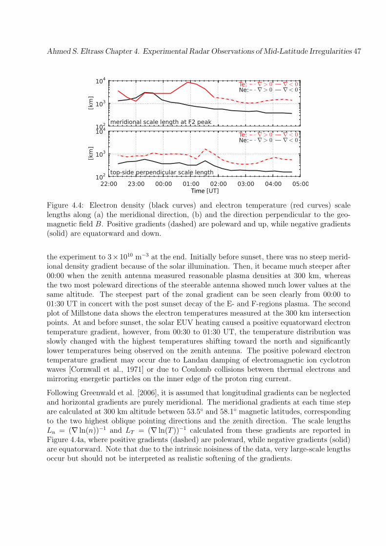
Ahmed S. Eltrass Chapter 4. Experimental Radar Observations of Mid-Latitude Irregularities 47
Time
Figure 4.4: Electron density (black curves) and electron temperature (red curves) scalelengths along (a) the meridional direction, (b) and the direction perpendicular to the geo-magnetic field B. Positive gradients (dashed) are poleward and up, while negative gradients(solid) are equatorward and down.
the experiment to 3×10¹⁰ m−3 at the end. Initially before sunset, there was no steep merid-ional density gradient because of the solar illumination. Then, it became much steeper after00:00 when the zenith antenna measured reasonable plasma densities at 300 km, whereasthe two most poleward directions of the steerable antenna showed much lower values at thesame altitude. The steepest part of the zonal gradient can be seen clearly from 00:00 to01:30 UT in concert with the post sunset decay of the E- and F-regions plasma. The secondplot of Millstone data shows the electron temperatures measured at the 300 km intersectionpoints. At and before sunset, the solar EUV heating caused a positive equatorward electrontemperature gradient, however, from 00:30 to 01:30 UT, the temperature distribution wasslowly changed with the highest temperatures shifting toward the north and significantlylower temperatures being observed on the zenith antenna. The positive poleward electrontemperature gradient may occur due to Landau damping of electromagnetic ion cyclotronwaves [Cornwall et al., 1971] or due to Coulomb collisions between thermal electrons andmirroring energetic particles on the inner edge of the proton ring current.
Following Greenwald et al. [2006], it is assumed that longitudinal gradients can be neglectedand horizontal gradients are purely meridional. The meridional gradients at each time stepare calculated at 300 km altitude between 53.5 and 58.1 magnetic latitudes, correspondingto the two highest oblique pointing directions and the zenith direction. The scale lengthsLn = (∇ ln(n))−1 and LT = (∇ ln(T ))−1 calculated from these gradients are reported inFigure 4.4a, where positive gradients (dashed) are poleward, while negative gradients (solid)are equatorward. Note that due to the intrinsic noisiness of the data, very large-scale lengthsoccur but should not be interpreted as realistic softening of the gradients.
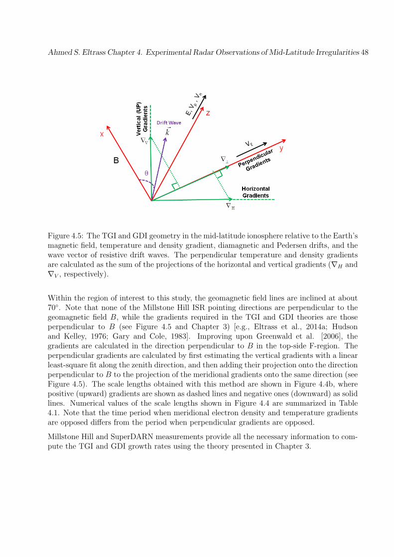
Ahmed S. Eltrass Chapter 4. Experimental Radar Observations of Mid-Latitude Irregularities 48
Figure 4.5: The TGI and GDI geometry in the mid-latitude ionosphere relative to the Earth’smagnetic field, temperature and density gradient, diamagnetic and Pedersen drifts, and thewave vector of resistive drift waves. The perpendicular temperature and density gradientsare calculated as the sum of the projections of the horizontal and vertical gradients (∇H and∇V , respectively).
Within the region of interest to this study, the geomagnetic field lines are inclined at about70. Note that none of the Millstone Hill ISR pointing directions are perpendicular to thegeomagnetic field B, while the gradients required in the TGI and GDI theories are thoseperpendicular to B (see Figure 4.5 and Chapter 3) [e.g., Eltrass et al., 2014a; Hudsonand Kelley, 1976; Gary and Cole, 1983]. Improving upon Greenwald et al. [2006], thegradients are calculated in the direction perpendicular to B in the top-side F-region. Theperpendicular gradients are calculated by first estimating the vertical gradients with a linearleast-square fit along the zenith direction, and then adding their projection onto the directionperpendicular to B to the projection of the meridional gradients onto the same direction (seeFigure 4.5). The scale lengths obtained with this method are shown in Figure 4.4b, wherepositive (upward) gradients are shown as dashed lines and negative ones (downward) as solidlines. Numerical values of the scale lengths shown in Figure 4.4 are summarized in Table4.1. Note that the time period when meridional electron density and temperature gradientsare opposed differs from the period when perpendicular gradients are opposed.
Millstone Hill and SuperDARN measurements provide all the necessary information to com-pute the TGI and GDI growth rates using the theory presented in Chapter 3.
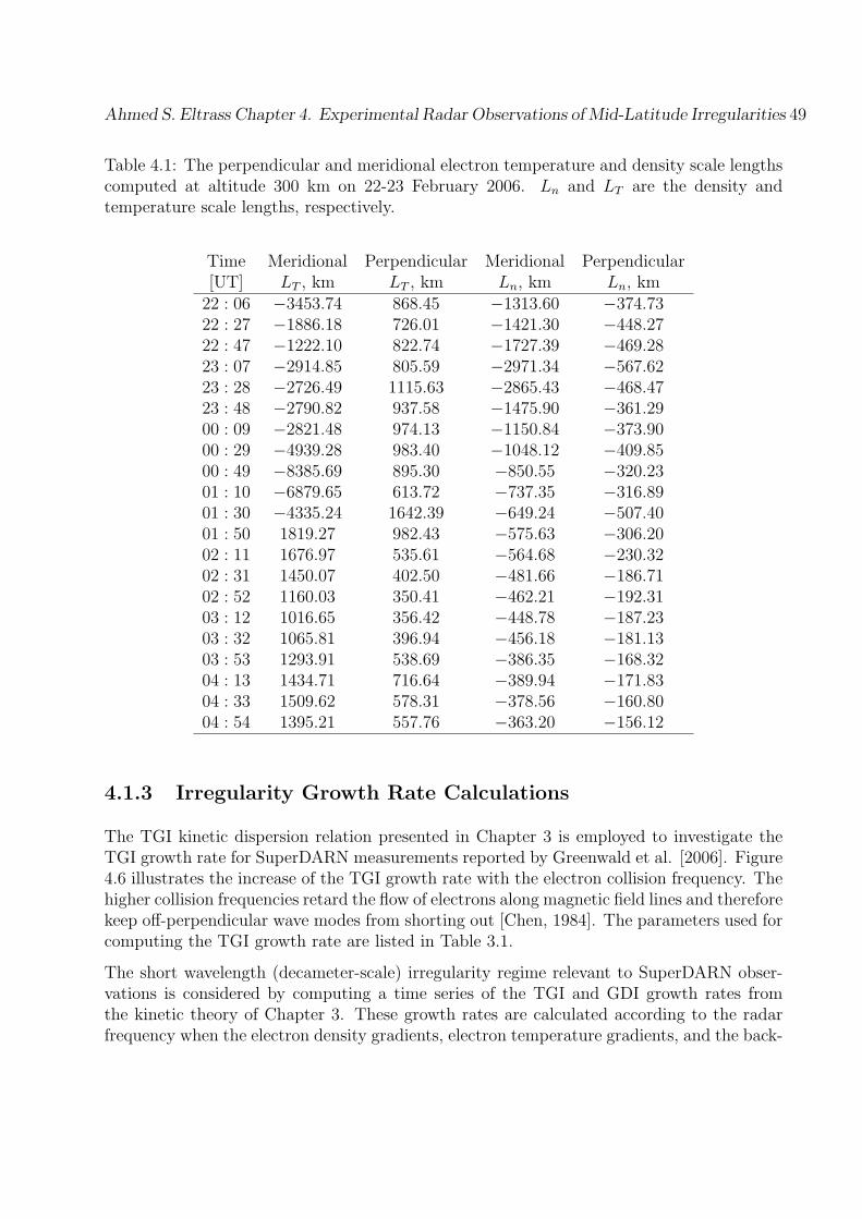
Ahmed S. Eltrass Chapter 4. Experimental Radar Observations of Mid-Latitude Irregularities 49
Table 4.1: The perpendicular and meridional electron temperature and density scale lengthscomputed at altitude 300 km on 22-23 February 2006. Ln and LT are the density andtemperature scale lengths, respectively.
Time Meridional Perpendicular Meridional Perpendicular[UT] LT , km LT , km Ln, km Ln, km22 : 06 −3453.74 868.45 −1313.60 −374.7322 : 27 −1886.18 726.01 −1421.30 −448.2722 : 47 −1222.10 822.74 −1727.39 −469.2823 : 07 −2914.85 805.59 −2971.34 −567.6223 : 28 −2726.49 1115.63 −2865.43 −468.4723 : 48 −2790.82 937.58 −1475.90 −361.2900 : 09 −2821.48 974.13 −1150.84 −373.9000 : 29 −4939.28 983.40 −1048.12 −409.8500 : 49 −8385.69 895.30 −850.55 −320.2301 : 10 −6879.65 613.72 −737.35 −316.8901 : 30 −4335.24 1642.39 −649.24 −507.4001 : 50 1819.27 982.43 −575.63 −306.2002 : 11 1676.97 535.61 −564.68 −230.3202 : 31 1450.07 402.50 −481.66 −186.7102 : 52 1160.03 350.41 −462.21 −192.3103 : 12 1016.65 356.42 −448.78 −187.2303 : 32 1065.81 396.94 −456.18 −181.1303 : 53 1293.91 538.69 −386.35 −168.3204 : 13 1434.71 716.64 −389.94 −171.8304 : 33 1509.62 578.31 −378.56 −160.8004 : 54 1395.21 557.76 −363.20 −156.12
4.1.3 Irregularity Growth Rate Calculations
The TGI kinetic dispersion relation presented in Chapter 3 is employed to investigate theTGI growth rate for SuperDARN measurements reported by Greenwald et al. [2006]. Figure4.6 illustrates the increase of the TGI growth rate with the electron collision frequency. Thehigher collision frequencies retard the flow of electrons along magnetic field lines and thereforekeep off-perpendicular wave modes from shorting out [Chen, 1984]. The parameters used forcomputing the TGI growth rate are listed in Table 3.1.
The short wavelength (decameter-scale) irregularity regime relevant to SuperDARN obser-vations is considered by computing a time series of the TGI and GDI growth rates fromthe kinetic theory of Chapter 3. These growth rates are calculated according to the radarfrequency when the electron density gradients, electron temperature gradients, and the back-
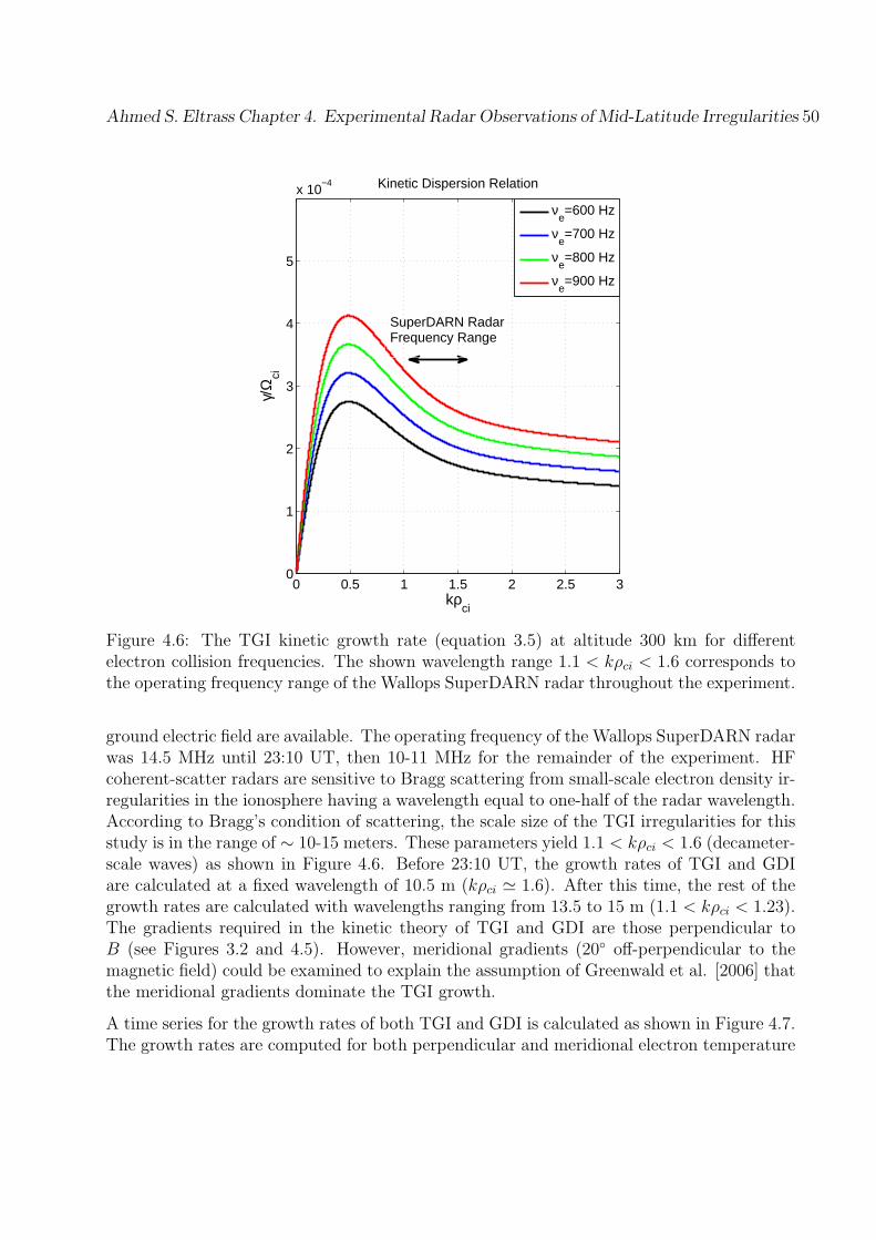
Ahmed S. Eltrass Chapter 4. Experimental Radar Observations of Mid-Latitude Irregularities 50
0 0.5 1 1.5 2 2.5 30
1
2
3
4
5
x 10−4 Kinetic Dispersion Relation
kρci
γ/Ω
ci
ν
e=600 Hz
νe=700 Hz
νe=800 Hz
νe=900 Hz
SuperDARN RadarFrequency Range
Figure 4.6: The TGI kinetic growth rate (equation 3.5) at altitude 300 km for differentelectron collision frequencies. The shown wavelength range 1.1 < kρci < 1.6 corresponds tothe operating frequency range of the Wallops SuperDARN radar throughout the experiment.
ground electric field are available. The operating frequency of the Wallops SuperDARN radarwas 14.5 MHz until 23:10 UT, then 10-11 MHz for the remainder of the experiment. HFcoherent-scatter radars are sensitive to Bragg scattering from small-scale electron density ir-regularities in the ionosphere having a wavelength equal to one-half of the radar wavelength.According to Bragg’s condition of scattering, the scale size of the TGI irregularities for thisstudy is in the range of ∼ 10-15 meters. These parameters yield 1.1 < kρci < 1.6 (decameter-scale waves) as shown in Figure 4.6. Before 23:10 UT, the growth rates of TGI and GDIare calculated at a fixed wavelength of 10.5 m (kρci ≃ 1.6). After this time, the rest of thegrowth rates are calculated with wavelengths ranging from 13.5 to 15 m (1.1 < kρci < 1.23).The gradients required in the kinetic theory of TGI and GDI are those perpendicular toB (see Figures 3.2 and 4.5). However, meridional gradients (20 off-perpendicular to themagnetic field) could be examined to explain the assumption of Greenwald et al. [2006] thatthe meridional gradients dominate the TGI growth.
A time series for the growth rates of both TGI and GDI is calculated as shown in Figure 4.7.The growth rates are computed for both perpendicular and meridional electron temperature
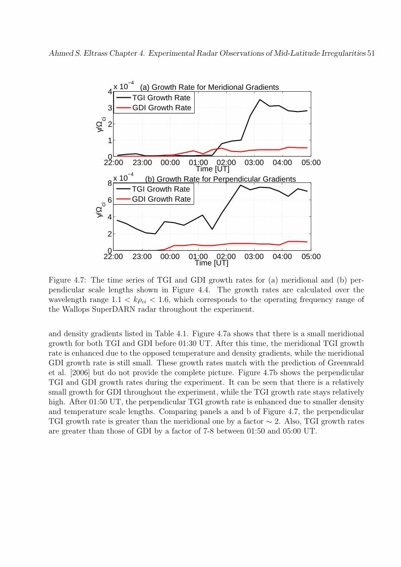
Ahmed S. Eltrass Chapter 4. Experimental Radar Observations of Mid-Latitude Irregularities 51
22:00 23:00 00:00 01:00 02:00 03:00 04:00 05:000
2
4
6
8x 10
−4
Time [UT]
γ/Ω
ci
(b) Growth Rate for Perpendicular Gradients
TGI Growth RateGDI Growth Rate
22:00 23:00 00:00 01:00 02:00 03:00 04:00 05:000
1
2
3
4x 10
−4
Time [UT]
γ/Ω
ci
(a) Growth Rate for Meridional Gradients
TGI Growth RateGDI Growth Rate
Figure 4.7: The time series of TGI and GDI growth rates for (a) meridional and (b) per-pendicular scale lengths shown in Figure 4.4. The growth rates are calculated over thewavelength range 1.1 < kρci < 1.6, which corresponds to the operating frequency range ofthe Wallops SuperDARN radar throughout the experiment.
and density gradients listed in Table 4.1. Figure 4.7a shows that there is a small meridionalgrowth for both TGI and GDI before 01:30 UT. After this time, the meridional TGI growthrate is enhanced due to the opposed temperature and density gradients, while the meridionalGDI growth rate is still small. These growth rates match with the prediction of Greenwaldet al. [2006] but do not provide the complete picture. Figure 4.7b shows the perpendicularTGI and GDI growth rates during the experiment. It can be seen that there is a relativelysmall growth for GDI throughout the experiment, while the TGI growth rate stays relativelyhigh. After 01:50 UT, the perpendicular TGI growth rate is enhanced due to smaller densityand temperature scale lengths. Comparing panels a and b of Figure 4.7, the perpendicularTGI growth rate is greater than the meridional one by a factor ∼ 2. Also, TGI growth ratesare greater than those of GDI by a factor of 7-8 between 01:50 and 05:00 UT.

Ahmed S. Eltrass Chapter 4. Experimental Radar Observations of Mid-Latitude Irregularities 52
4.1.4 Discussion
The mid-latitude decameter-scale ionospheric irregularities are generally observed on thenightside. During the day, the observation of these irregularities is controlled by both theelectrical conductance of the underlying ionosphere and the F-region electron density. Theabsence of these irregularities during the day may occur since the perturbation charges of theF-region may be shorted-out by a current flow to the E-region [Vickrey and Kelley, 1982].However, even if they exist during the daytime, the electron density variation can affectsignal propagation in such a way that the radar signals do not encounter the irregularitiesat all [Kane et al., 2012].
A complete comparison of TGI and GDI is done for SuperDARN observations at the night-side plasmapause reported by Greenwald et al. [2006]. As shown in Figure 4.7, the TGIand GDI growth rates for this experiment are calculated as a function of universal timecorresponding to both perpendicular and meridional gradients. Figure 4.7 illustrates thatthere is a relatively small growth for GDI throughout the experiment, while the TGI growthrate stays relatively high. The perpendicular TGI growth rates are greater than those ofGDI up to a factor of ∼ 8. This suggests that the observed decameter-scale ionosphericirregularities are produced by the TGI or a cascade product from it, while the GDI playsa relatively minor role in the generation of these irregularities. The GDI does not have asignificant role in the primary irregularity generation, however, it should not be ruled outat this time that turbulent cascade processes of both TGI and GDI may contribute to theobserved irregularities. The calculations here show the TGI growth exceeds that of the GDIgrowth in the wavelength of observations (10-15 m), as well as in the long wavelength regime(km). A cascade process may occur from km-scale irregularity structures down to the ob-served decameter-scale irregularities. Such critical physics, e.g., wave cascading, can mosteffectively be investigated with nonlinear plasma simulation models. The simulation resultswill be discussed in Chapter 5.
Figure 4.4a revealed opposed meridional temperature and density gradients at the night-side mid-latitude ionosphere after 01:30 UT. Initially, there was no steep meridional densitygradient due to solar illumination of the F-region, but it became much steeper after 00:00UT because of F-region sunset. Before sunset, solar heating caused a positive equatorwardelectron temperature gradient. In the time interval from 01:00-02:00 UT, the meridionalelectron temperature gradient changed direction and the positive gradient in electron tem-perature reversed from equatorward to poleward. The positive poleward meridional electrontemperature gradient may have occurred due to Coulomb collisions between thermal elec-trons and trapped energetic particles in the poleward region, while the reduction of electrontemperatures in the equatorward region was due to post-sunset cooling [Greenwald et al.,2006].
The perpendicular temperature and density gradients at the nightside mid-latitude iono-sphere are opposite throughout the experiment, while the meridional gradients are opposedonly after 01:30 UT. The TGI growth rate is largely affected by the variations of the temper-
Ahmed S. Eltrass Chapter 4. Experimental Radar Observations of Mid-Latitude Irregularities 53
ature and density gradients. As shown in Table 4.1 and Figure 4.4, the perpendicular andmeridional scale lengths become much smaller after 01:30 UT, causing the large enhance-ment of the TGI growth rate shown in Figure 4.7. Panels a and b of Figure 4.7 show thatthe perpendicular TGI growth rate is greater than the meridional one and dominates forthe duration of the experiment, while the meridional TGI growth starts only after 01:30.The perpendicular TGI growth rate challenges the suggestion of Greenwald et al. [2006]that the dusk scatter associated with the GDI [Ruohoniemi et al., 1988] may account for theirregularities observed between 00:00 and 01:40 UT. The dusk scatter appears immediatelyafter the local sunset and does not typically connect with scatter from other irregularitytypes in a smooth transition such as seen in Figure 4.2. The continuity of the scatter shownin Figure 4.2 along with the growth rate calculations suggest that the TGI is the most likelygeneration mechanism for the irregularities observed during the experiment and the GDI isexpected to play a relatively minor role in irregularity generation. The TGI growth rate canalso explain the observed low-velocity SAIS between 00:10 and 05:00 UT shown in Figure4.2.
The TGI growth may not be observed by the Wallops SuperDARN radar before sunsetdue to two distinct reasons. The first is the signal propagation effects in which the radarsignals encounter these irregularities under unsuitable magnetic aspect conditions or donot encounter them at all [e.g., Davies, 1990]. Using a ray-tracing model coupled withthe International Reference Ionosphere (IRI) [de Larquier et al., 2014], the propagationconditions are shown to be favorable for observing decameter-scale irregularities in the F-region before sunset. This suggests that propagation aspect conditions did not limit theobservation of irregularity backscatter. The second potential explanation is the high E-region conductivity, which may short-out the F-region TGI electric fields before and aroundsunset in spite of favorable growth conditions for the TGI. After sunset, the TGI irregularitywere able to grow for the remainder of the experiment as suggested by the TGI growth ratesshown in Figure 4.7. The role of the E-region in shorting out F-region electrostatic fieldsbefore sunset raises the importance of knowing the wavelength of these irregularities. Theirregularities with scale sizes smaller than 1 km are greatly attenuated when mapped fromthe F- to the E-region [e.g., Farley, 1959; Kelley, 2009]. This implies that for the E-region tobe responsible for shorting out the F-region TGI electric fields before and around sunset, theirregularities should be in the km-scale. This result suggests that a turbulent cascade processmay occur from km-scale primary TGI irregularity structures down to the decameter-scaleirregularities. Such physics will be investigated with plasma simulation models in Chapter5.
Ahmed S. Eltrass Chapter 4. Experimental Radar Observations of Mid-Latitude Irregularities 54
4.2 Comparison with Disturbed-Time Plasma Wave
Irregularities
The storm-time ionospheric irregularities at mid-latitudes are sufficiently strong to causesignal power fluctuations, known as ionospheric scintillation, in transionospheric satellitetransmissions such as the Global Positioning System (GPS) [e.g., Basu et al., 2001; Ledv-ina et al., 2002; Mishin et al., 2003]. This raises the importance of knowing the causeand distribution of these ionospheric plasma irregularities to maintain the performance ofsatellite-ground data transmission. Potential space weather applications have paid the at-tention to the spatial temporal variability of the mid-latitude sub-auroral ionosphere duringmagnetic storm periods [e.g., Mishin et al., 2003; Ledvina et al., 2002; Foster et al., 2002;Basu et al., 2001, 2008]. During disturbed geomagnetic conditions, large regions hostingan ionospheric density gradient exist in the evening sector at sub-auroral latitudes in thetop-side ionosphere [e.g., Coster et al., 2005; Spiro et al., 1979; Evans et al., 1983; Andersonet al., 1991, 1993]. These density gradients are often associated with streams of enhancedplasma convection known as Sub-Auroral Plasma Streams (SAPS) [e.g., Foster and Burke,2002], and with Storm-Enhanced Densities (SEDs) [e.g., Erickson et al., 2002]. Several pre-vious studies investigated the characteristics of SAPS using the measurements of MillstoneHill ISR during disconnected events over a span of two solar cycles starting in 1979 [e.g., Yehet al., 1991; Erickson et al., 2002]. Satellite measurements reveal the existence of wave-likestructures embedded within the SAPS [Mishin et al., 2002, 2003, 2004; Streltsov and Mishin,2003; Streltsov and Foster, 2004; Foster et al., 2004]. Basu et al. [2001] and Ledvina et al.[2002] reported intense mid-latitude UHF and L1-band scintillations within structured SAPSover the eastern continental United States. Mishin et al. [2004] showed that strong SAPSwave structures and irregular plasma density troughs are associated with strong oppositetemperature and density gradients, which represent the precise conditions required for thedevelopment of the F-region Temperature Gradient Instability (TGI) [e.g., Hudson and Kel-ley, 1976; Eltrass et al., 2014a; Eltrass and Scales, 2014]. Satellite observations also indicatethe presence of small-scale density, electric field, velocity, and electron temperature struc-tures in SAPS storm-time mid-latitude trough structures [e.g., Mishin et al., 2003]. Keskinenet al. [2004] suggested that the Temperature Gradient Instability (TGI) in association withthe Gradient Drift Instability (GDI) could be responsible for generating these small-scalestructures in the trough wall region.
4.2.1 SuperDARN Observations
During the nights of 15-16 October 2014 (quiet geomagnetic conditions Kp < 2) and 10-11October 2014 (active geomagnetic conditions 3 < Kp ≤ 4), the Blackstone SuperDARNradar (37.10 N, 282.05 E) and the Millstone Hill Incoherent Scatter Radar (ISR) (42.6
N, 288.5 E) were running co-located observations of sub-auroral ionospheric irregularities.

Ahmed S. Eltrass Chapter 4. Experimental Radar Observations of Mid-Latitude Irregularities 55
Figure 4.8: Backscatter echoes from the Blackstone SuperDARN radar on the nights ofOctober 15-16 and October 10-11, 2014. Backscatter power and line-of-sight Doppler velocitymeasured along beam 13 during the two events are shown in panels (a, c) and (b, d),respectively.
The Blackstone SuperDARN radar was operating in a standard 16-position azimuth-scanningmode with a dwell time of 3 seconds in each azimuth direction and a scan repetition timeof 60 seconds. The observations during the two events were predominantly from F-regiondecameter-scale ionospheric irregularities extending from 500-1400 km in range from Black-stone radar, relevant to latitudes from 52 to 60.
Figure 4.8 shows the backscatter power and line-of-sight Doppler velocity observed by theBlackstone SuperDARN radar through the two events along beam 13 on the nights of Oc-tober 15-16 (quiet-time) and October 10-11 (disturbed-time), 2014. Figure 4.8a-c showsthe relative backscattered power in dB, while Figure 4.8b-d shows the line-of-sight Dopplervelocity in m/s. The line-of-sight Doppler velocities of ionospheric scatter are L-shell fittedassuming a purely zonal plasma flow [Ruohoniemi et al., 1989]. The irregularity Doppler
Ahmed S. Eltrass Chapter 4. Experimental Radar Observations of Mid-Latitude Irregularities 56
velocities are calculated at 300 km altitude from 00:00 to 08:00 UT on both events, showingthat the plasma drift speed in the plasmapause is quite small (< 50 m/s) during quiet-timebut relatively high during active periods (< 150 m/s). The observations during the twoevents show both types of backscatter, ground and ionospheric scatter. First, the scatterfrom higher magnetic latitudes over the time interval 00:00 to 02:00 UT is ground backscat-ter. After 02:00, the radar begins to observe ionospheric scatter over latitudes from 54 to60 on most of the radar beams. The ionospheric irregularities responsible for the observedscatter are seen in the top-side F-region ionosphere and extend uniformly across the radarfield-of-view.
4.2.2 Millstone Hill ISR Measurements
The data from the Millstone Hill Incoherent Scatter Radar (ISR) are analyzed to determinethe physical mechanisms responsible for the observed ionospheric irregularities during thetwo events. For this experiment, overhead measurements are obtained with the 68 m zenith-pointing antenna and oblique measurements were obtained with the 46 m steerable dishto provide quantitative estimates of vertical and horizontal ionospheric structure in the F-region ionosphere within the field-of-view of the Blackstone SuperDARN radar. The gradientmeasurement region is centered on a point with geodetic latitude and longitude coordinatesof (43.55, −84.89), intersecting beam 13 of the Blackstone system at 300 km altitude. Thealtitude of 300 km is chosen to be close to the F-region peak altitude, where the Signal-to-Noise Ratio (SNR) should be maximum. Using Millstone Hill steerable antenna, elevationscanning is done from 8 to 12 at a fixed azimuth of −80, while azimuth scanning isperformed from −105 to 60 at a fixed elevation of 10. The zenith direction is alternatedbetween each look directions, giving its data a time resolution of 5 min compared to 30 minfor other pointing directions. Slow azimuth and elevation scans are performed around the300 km point to provide the horizontal and vertical structure.
Combining measurements from the zenith scans and the azimuth scans, the Millstone HillISR data are used to calculate the horizontal and vertical gradients. Within the region ofinterest to this study, the geomagnetic field lines are inclined at about 70. The electrondensity and temperature gradients are calculated in the direction perpendicular to B in thetop-side F-region by first estimating the vertical gradients with a linear least-square fit alongthe zenith direction, and then adding their projection onto the direction perpendicular to Bto the projection of the horizontal gradients onto the same direction (see Figure 4.5). Theperpendicular density and temperature scale lengths for both events are shown in Figure4.9a-b, where positive (upward) gradients are shown as dashed lines and negative gradients(downward) as solid lines. It can be noted that the quiet-time scale lengths (> 300 km) arelarger than those obtained during the disturbed-time event (> 100 km).
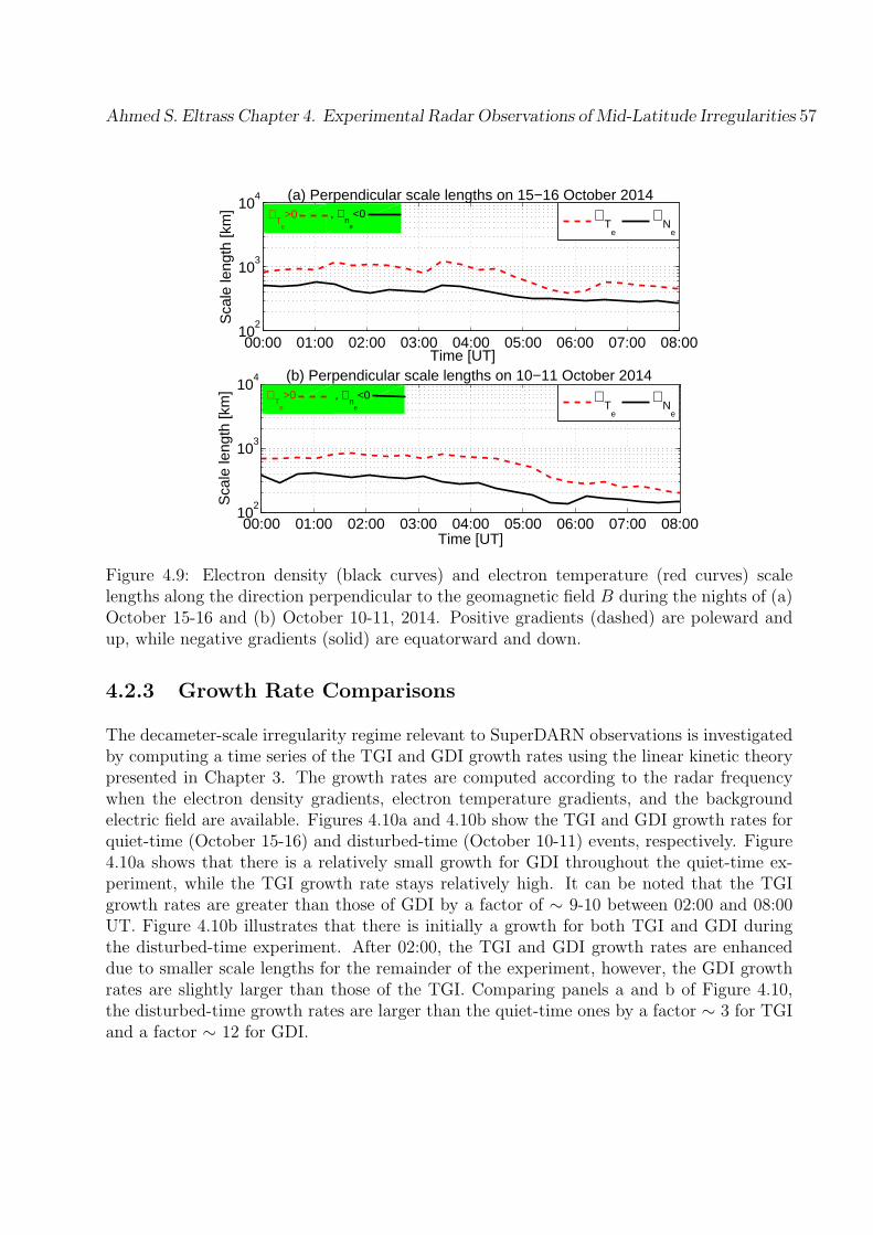
Ahmed S. Eltrass Chapter 4. Experimental Radar Observations of Mid-Latitude Irregularities 57
00:00 01:00 02:00 03:00 04:00 05:00 06:00 07:00 08:0010
2
103
104
Time [UT]
Sca
le le
ngth
[km
]
(a) Perpendicular scale lengths on 15−16 October 2014
00:00 01:00 02:00 03:00 04:00 05:00 06:00 07:00 08:0010
2
103
104
Time [UT]
Sca
le le
ngth
[km
]
(b) Perpendicular scale lengths on 10−11 October 2014
∇T
e
∇N
e
∇T
e
∇N
e
, ∇n
e
<0
∇T
e
>0 , ∇n
e
<0
∇T
e
>0
Figure 4.9: Electron density (black curves) and electron temperature (red curves) scalelengths along the direction perpendicular to the geomagnetic field B during the nights of (a)October 15-16 and (b) October 10-11, 2014. Positive gradients (dashed) are poleward andup, while negative gradients (solid) are equatorward and down.
4.2.3 Growth Rate Comparisons
The decameter-scale irregularity regime relevant to SuperDARN observations is investigatedby computing a time series of the TGI and GDI growth rates using the linear kinetic theorypresented in Chapter 3. The growth rates are computed according to the radar frequencywhen the electron density gradients, electron temperature gradients, and the backgroundelectric field are available. Figures 4.10a and 4.10b show the TGI and GDI growth rates forquiet-time (October 15-16) and disturbed-time (October 10-11) events, respectively. Figure4.10a shows that there is a relatively small growth for GDI throughout the quiet-time ex-periment, while the TGI growth rate stays relatively high. It can be noted that the TGIgrowth rates are greater than those of GDI by a factor of ∼ 9-10 between 02:00 and 08:00UT. Figure 4.10b illustrates that there is initially a growth for both TGI and GDI duringthe disturbed-time experiment. After 02:00, the TGI and GDI growth rates are enhanceddue to smaller scale lengths for the remainder of the experiment, however, the GDI growthrates are slightly larger than those of the TGI. Comparing panels a and b of Figure 4.10,the disturbed-time growth rates are larger than the quiet-time ones by a factor ∼ 3 for TGIand a factor ∼ 12 for GDI.
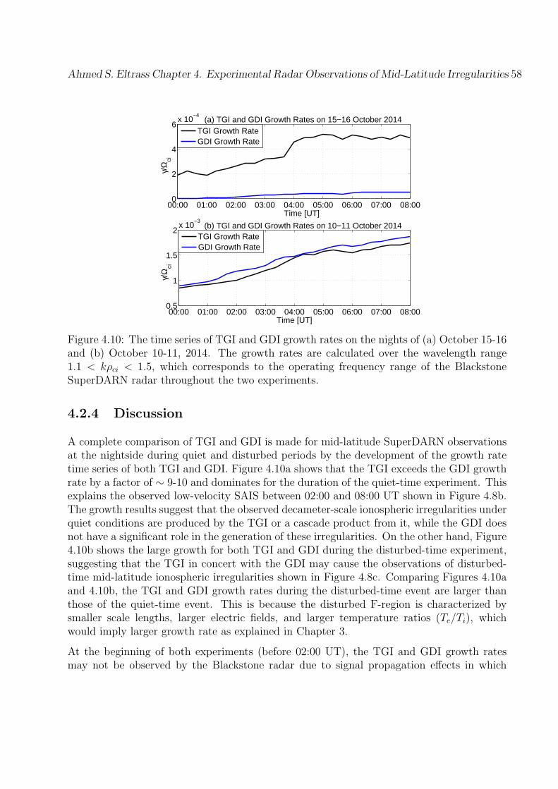
Ahmed S. Eltrass Chapter 4. Experimental Radar Observations of Mid-Latitude Irregularities 58
00:00 01:00 02:00 03:00 04:00 05:00 06:00 07:00 08:000.5
1
1.5
2x 10
−3
Time [UT]
γ/Ω
ci
(b) TGI and GDI Growth Rates on 10−11 October 2014
TGI Growth RateGDI Growth Rate
00:00 01:00 02:00 03:00 04:00 05:00 06:00 07:00 08:000
2
4
6x 10
−4
Time [UT]
γ/Ω
ci
(a) TGI and GDI Growth Rates on 15−16 October 2014
TGI Growth RateGDI Growth Rate
Figure 4.10: The time series of TGI and GDI growth rates on the nights of (a) October 15-16and (b) October 10-11, 2014. The growth rates are calculated over the wavelength range1.1 < kρci < 1.5, which corresponds to the operating frequency range of the BlackstoneSuperDARN radar throughout the two experiments.
4.2.4 Discussion
A complete comparison of TGI and GDI is made for mid-latitude SuperDARN observationsat the nightside during quiet and disturbed periods by the development of the growth ratetime series of both TGI and GDI. Figure 4.10a shows that the TGI exceeds the GDI growthrate by a factor of ∼ 9-10 and dominates for the duration of the quiet-time experiment. Thisexplains the observed low-velocity SAIS between 02:00 and 08:00 UT shown in Figure 4.8b.The growth results suggest that the observed decameter-scale ionospheric irregularities underquiet conditions are produced by the TGI or a cascade product from it, while the GDI doesnot have a significant role in the generation of these irregularities. On the other hand, Figure4.10b shows the large growth for both TGI and GDI during the disturbed-time experiment,suggesting that the TGI in concert with the GDI may cause the observations of disturbed-time mid-latitude ionospheric irregularities shown in Figure 4.8c. Comparing Figures 4.10aand 4.10b, the TGI and GDI growth rates during the disturbed-time event are larger thanthose of the quiet-time event. This is because the disturbed F-region is characterized bysmaller scale lengths, larger electric fields, and larger temperature ratios (Te/Ti), whichwould imply larger growth rate as explained in Chapter 3.
At the beginning of both experiments (before 02:00 UT), the TGI and GDI growth ratesmay not be observed by the Blackstone radar due to signal propagation effects in which
Ahmed S. Eltrass Chapter 4. Experimental Radar Observations of Mid-Latitude Irregularities 59
the radar signals encounter these irregularities under unsuitable magnetic aspect conditionsor do not encounter them at all [e.g., Davies, 1990]. Another reason for the delay betweensunset (00:00 UT) and irregularity observations (02:00 UT) could be the E-region as thecontrolling factor for irregularity growth. The reasonable agreement between experimentaland theoretical results of this study suggests that a TGI turbulent cascade is the most likelygeneration mechanism for the quiet-time irregularities that cause the observed low-velocitySAIS, while turbulent cascade processes of both TGI and GDI may cause the observationsof ionospheric irregularities during disturbed geomagnetic conditions. This lends furthersupport to the belief that the E-region may be responsible for shorting out the F-region TGIand GDI electric fields before and around sunset and ultimately resulting in irregularitysuppression.
Chapter 5
Simulation of TGI Irregularities inthe Mid-Latitude Ionosphere
5.1 Computational Modeling
Although the linear theory of Chapter 3 provides the insight for the initial linear growth of theplasma instability process, it cannot fully describe the nonlinearly saturated behavior and theassociated particle transport. When the plasma waves are observed with radars, they havealready evolved into a nonlinear state. Such nonlinear evolution, e.g., wave cascading, is mostlikely critical for ultimately determining the scale size of the irregularities observed by theradar observations [Eltrass et al., 2014a]. The physics associated with plasma instabilitiescan most effectively be investigated with plasma simulation models. The computationalplasma simulation is an efficient tool to provide physical insight and predictions for plasmainstabilities. Plasma simulations comprise two general methods based on kinetic and fluiddescription. This classification can be divided further into tree types of plasma simulationas following:
• Fluid and magnetohydrodynamic codes: the fluid simulation is the oldest and simplestmethod in plasma simulation. The equations in the fluid formulation treat each plasmaspecies as a moving fluid ignoring the important wave and particle interaction. The fluidsimulation approach neglects the identity of individual particles and only the collective natureof plasma particles is considered. Due to the nature of fluid treatment, fluid simulationmethods are most appropriate for scale lengths much larger than the ion gyro-radius ρciand time scales larger than the inverse of the ion gyro-period Ω−1
ci (see Figure 5.1). In amagnetized plasma, the fluid formulation is replaced by magnetohydrodynamic equations tosimulate the plasma as a single fluid.
• Particle-In-Cell (PIC) codes: the PIC simulation is an efficient approach for simulatingsmall time scales and small spatial scales with full kinetic effects. As shown in Figure 5.1, the
60

Ahmed S. Eltrass Chapter 5. Simulation of TGI Irregularities in the Mid-Latitude Ionosphere 61
Figure 5.1: Time and space scales for different plasma simulation methods.
time scales for PIC codes are typically on the order of electron plasma period, while the PICspace scales are on the order of the Debye length λD. In this approach, the plasma behavioris modeled by following the motion of a large number of charged particles interacting witheach other and with externally applied fields. Note that each particle has a set of attributessuch as mass, position, charge, and momentum. Equations included in the PIC simulationare the discretized version of Maxwell’s equations, Newton’s second law of motion, and theLorentz force equation (see Appendix C).
• Hybrid codes: this simulation approach is appropriate for scales larger than ρci and Ω−1ci
but shorter than the fluid scales (intermediate scales as shown in Figure 5.1), in which amixing of the particle-like and the fluid-like behavior occurs. In the hybrid codes, fluid andparticle treatments are applied to different components of a given plasma, i.e., electrons aretreated as a massless fluid, while the ions and neutrals are treated as simulation particleswith kinetic effects [Winske et al., 2003]. Hybrid codes allow the modeling of the ionosphericplasma irregularities at ion scales (ion gyro-radius and ion inertial spatial scales) but they donot solve processes at electron scales (electron gyro-radius and electron Debye length scales).
Of the three types of plasma simulations described above, the Particle-In-Cell (PIC) sim-ulation is the suitable approach for studying the nonlinear evolution of decameter-scaleionospheric irregularities observed by SuperDARN radars (which is the focus of this study).
Ahmed S. Eltrass Chapter 5. Simulation of TGI Irregularities in the Mid-Latitude Ionosphere 62
5.1.1 Basic Formulation of Plasma Simulation
The Vlasov equation describes the kinetic plasma evolution as follows:
∂fj∂t
+ υ · ∇fj +qjmj
(E + υ ×B) · ∂fj∂υ
= 0 (5.1)
where fj(x, υ) is the velocity distribution of the jth plasma species, qj is the species charge,and mj is the species mass. The electric field E and the magnetic field B are obtainedusing Maxwell’s equations, which contain the sources terms from the moments of all plasmaspecies.
The Maxwell’s equations in term of the velocity distribution can be expressed as:
∇× E = −∂B∂t
(5.2)
∇×B = µ
(n∑
j=1
qj
∫fjdυ + ϵ
∂E
∂t
)(5.3)
ϵ∇ · E =n∑
j=1
qj
∫fjdυ (5.4)
∇ ·B = 0 (5.5)
where ϵ is the medium permittivity and µ is the medium permeability. If all charged particlesin a plasma are free, then ϵ ≃ ϵ0 and µ = µ0, where the subscript 0 denotes the quantity invacuum. The Vlasov equation along with Maxwell’s equations make up a complete descrip-tion for the kinetic behavior of the plasma evolution. This set of equations could be furthersimplified by electrostatic field approximation (no magnetic variations with time) dependingon different applications. The Particle-In-Cell (PIC) method is a kinetic treatment adoptedto solve these equations.
5.1.2 Electrostatic Field Approximation
The ionosphere is a low-β plasma (β << 1), where β is the ratio of plasma pressure tomagnetic pressure. The ionospheric magnetic field is sufficiently large such that the magneticfield variations can be neglected at all frequencies (∂B/∂t = 0). Based on the Faraday’s law(∇ × E = 0), the electric field can be written as E = −∇Φ, where Φ is the electrostatic
Ahmed S. Eltrass Chapter 5. Simulation of TGI Irregularities in the Mid-Latitude Ionosphere 63
potential. Using this result and substituting into the Gauss’s law (equation 5.4), the Poisson’sequation can be written as:
ϵ0∇2Φ = −n∑
j=1
qjnj (5.6)
Since small charge differences in the ionosphere can cause large electric fields, the ionosphericplasma should exhibit charge neutrality ∂ρ/∂t ≈ 0, where ρ is the charge density and J isthe current density. This implies that ∇ · J = 0 and that the number of electrons per unitvolume should be equal to the number of positive ions of all types. Also, the conductioncurrent is much larger than the vacuum displacement current (ϵ0∂E/∂t) for all frequenciesof interest. Therefore, the displacement current in the Ampere’s law (equation 5.3) can beneglected. Now, the Maxwell’s equations for the electrostatic treatment can be written as:
E = −∇Φ (5.7)
∇×B = µ
n∑j=1
qj
∫fjdυ = µJ (5.8)
ϵ∇ · E =n∑
j=1
qj
∫fjdυ = ρ (5.9)
∇ ·B = 0 (5.10)
These equations along with Vlasov equation form the basis for the electrostatic treatmentof the ionospheric plasma. Note that a pure electrostatic model is computationally morefeasible than a fully electromagnetic model and consequently provides more resolution of theelectrostatic parametric processes that produce ionospheric plasma instabilities. In essenceof the above, the electrostatic approximation is used in this study to model the mid-latitudeionospheric TGI.
5.2 Plasma Simulation Model
The application of particle simulation to the study of nonlinear evolution of drift waves hasa relatively long history [Lee and Okuda, 1978]. The conventional particle models basedon the guiding center electrons and gyrating (Vlasov) ion processes [Lee and Okuda, 1978]are not practical for studying low-frequency drift waves. The reason is that high-frequencyspace-charge waves increase the noise level in the simulation plasma, which can lead to the
Ahmed S. Eltrass Chapter 5. Simulation of TGI Irregularities in the Mid-Latitude Ionosphere 64
suppression of irregularity growth of the low-frequency drift waves. Also, when the saturationamplitude of the instability is lower than the noise level, the nonlinear physics can also belost [Lee, 1987]. The conventional models [Lee and Okuda, 1978], limited by large noise levelas well as by small time steps and small grid sizes, are not suitable for simulating the TGInonlinear evolution relevant to SuperDARN observations.
The development of the gyro-kinetic particle simulation method [Lee, 1987] was motivatedto be able to investigate the nonlinear kinetic effects (for example, the electron behavior indrift waves). The gyro-kinetic model provides a way to separate the spatial scales for thebackground inhomogeneity from those associated with the perturbations [Lee, 1987]. In doingthis, the density and temperature gradients become input parameters for the simulation.This allows the study of steady-state drift wave turbulence problems through the eliminationof time and spatial scales associated with global transport from the simulation [Lee, 1983].This reflects the realistic experimental situation for SuperDARN observations, where thedensity and temperature gradients, which drive the TGI, tend to persist as a quasi-staticprofiles caused by the continuous replenishment of the plasma. The turbulence consideredis driven by diamagnetic drifts (from both temperature and density gradients) to simulatereplenishing gradients. This model is also appropriate for shallow density gradients 1
ndndx>> λ
(suitable for SuperDARN decameter-scale observations).
5.2.1 Gyro-Kinetic Simulation Model
In order to investigate the nonlinear evolution of the Temperature Gradient Instability (TGI)in the mid-latitude ionosphere, the gyro-kinetic simulation model, which contains the non-linearities relevant to F-region irregularities, is employed. The gyro-averaged Vlasov-Poissonsystem of equations are solved using particle simulation methods, in which the particle gy-ration is removed from the equations of motion [Lee, 1983; Dubin et al., 1983]. This modelallows the use of time steps longer than the gyro-period Ω−1
ci (and the plasma period ω−1pe )
and grid sizes longer than the Debye length (λD) [Lee, 1987]. Therefore, the computationalefficiency for the gyro-kinetic approach is much improved in the time step and grid size re-quirements compared with conventional simulations [Lee and Okuda, 1978]. The low noiselevel of this model provides the possibility of simulating a much larger volume of plasma forthe same number of particles [Krommes et al., 1986].
The simulation geometry used in the investigation of the TGI gyro-kinetic approach is shownin Figure 5.2. The magnetic field is assumed to be nearly parallel to the z-direction andlies in the x-z plane described by angle θB as shown. The positive y-axis is the direction ofthe density gradient, while the negative y-axis is the direction of the temperature gradient.The drift waves propagate primarily in the x-direction because computations show that themaximum TGI growth rate is obtained where the wave vector of resistive drift waves isalmost perpendicular to the magnetic field.
As noted previously in Chapter 4, Eltrass et al. [2014a, b] identified the presence of
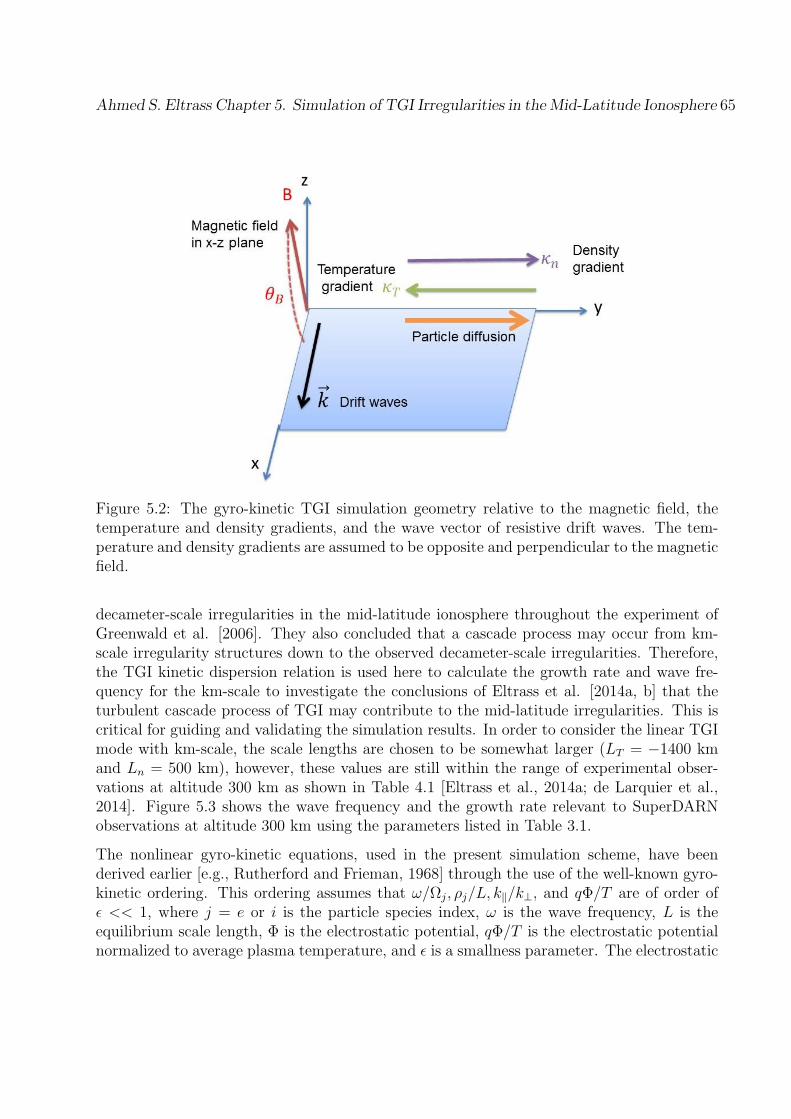
Ahmed S. Eltrass Chapter 5. Simulation of TGI Irregularities in the Mid-Latitude Ionosphere 65
Figure 5.2: The gyro-kinetic TGI simulation geometry relative to the magnetic field, thetemperature and density gradients, and the wave vector of resistive drift waves. The tem-perature and density gradients are assumed to be opposite and perpendicular to the magneticfield.
decameter-scale irregularities in the mid-latitude ionosphere throughout the experiment ofGreenwald et al. [2006]. They also concluded that a cascade process may occur from km-scale irregularity structures down to the observed decameter-scale irregularities. Therefore,the TGI kinetic dispersion relation is used here to calculate the growth rate and wave fre-quency for the km-scale to investigate the conclusions of Eltrass et al. [2014a, b] that theturbulent cascade process of TGI may contribute to the mid-latitude irregularities. This iscritical for guiding and validating the simulation results. In order to consider the linear TGImode with km-scale, the scale lengths are chosen to be somewhat larger (LT = −1400 kmand Ln = 500 km), however, these values are still within the range of experimental obser-vations at altitude 300 km as shown in Table 4.1 [Eltrass et al., 2014a; de Larquier et al.,2014]. Figure 5.3 shows the wave frequency and the growth rate relevant to SuperDARNobservations at altitude 300 km using the parameters listed in Table 3.1.
The nonlinear gyro-kinetic equations, used in the present simulation scheme, have beenderived earlier [e.g., Rutherford and Frieman, 1968] through the use of the well-known gyro-kinetic ordering. This ordering assumes that ω/Ωj, ρj/L, k∥/k⊥, and qΦ/T are of order ofϵ << 1, where j = e or i is the particle species index, ω is the wave frequency, L is theequilibrium scale length, Φ is the electrostatic potential, qΦ/T is the electrostatic potentialnormalized to average plasma temperature, and ϵ is a smallness parameter. The electrostatic
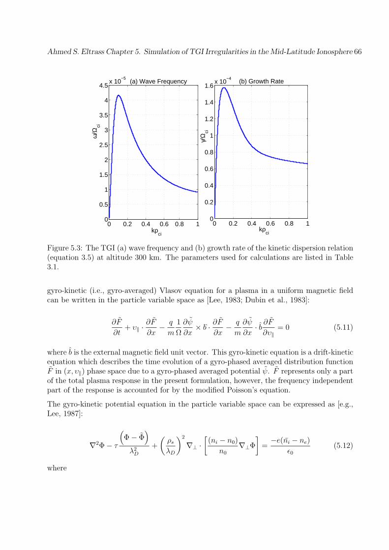
Ahmed S. Eltrass Chapter 5. Simulation of TGI Irregularities in the Mid-Latitude Ionosphere 66
0 0.2 0.4 0.6 0.8 10
0.5
1
1.5
2
2.5
3
3.5
4
4.5x 10
−5
kρci
ω/Ω
ci
(a) Wave Frequency
0 0.2 0.4 0.6 0.8 10
0.2
0.4
0.6
0.8
1
1.2
1.4
1.6x 10
−4
kρci
γ/Ω
ci
(b) Growth Rate
Figure 5.3: The TGI (a) wave frequency and (b) growth rate of the kinetic dispersion relation(equation 3.5) at altitude 300 km. The parameters used for calculations are listed in Table3.1.
gyro-kinetic (i.e., gyro-averaged) Vlasov equation for a plasma in a uniform magnetic fieldcan be written in the particle variable space as [Lee, 1983; Dubin et al., 1983]:
∂F
∂t+ υ∥ ·
∂F
∂x− q
m
1
Ω
∂ψ
∂x× b · ∂F
∂x− q
m
∂ψ
∂x· b ∂F∂υ∥
= 0 (5.11)
where b is the external magnetic field unit vector. This gyro-kinetic equation is a drift-kineticequation which describes the time evolution of a gyro-phased averaged distribution functionF in (x, υ∥) phase space due to a gyro-phased averaged potential ψ. F represents only a partof the total plasma response in the present formulation, however, the frequency independentpart of the response is accounted for by the modified Poisson’s equation.
The gyro-kinetic potential equation in the particle variable space can be expressed as [e.g.,Lee, 1987]:
∇2Φ− τ
(Φ− Φ
)λ2D
+
(ρsλD
)2
∇⊥ ·[(ni − n0)
n0
∇⊥Φ
]=
−e(ni − ne)
ϵ0(5.12)
where
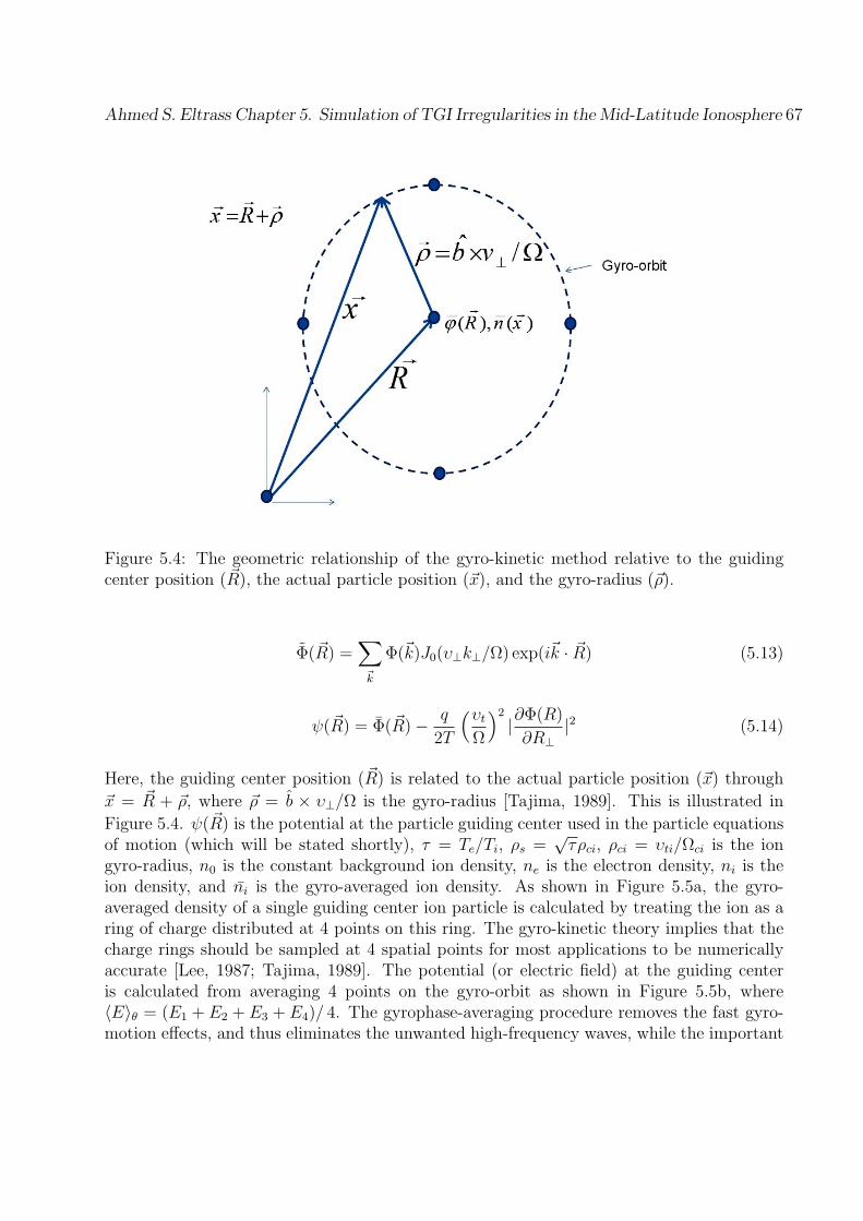
Ahmed S. Eltrass Chapter 5. Simulation of TGI Irregularities in the Mid-Latitude Ionosphere 67
Figure 5.4: The geometric relationship of the gyro-kinetic method relative to the guidingcenter position (R), the actual particle position (x), and the gyro-radius (ρ).
Φ(R) =∑k
Φ(k)J0(υ⊥k⊥/Ω) exp(ik · R) (5.13)
ψ(R) = Φ(R)− q
2T
(υtΩ
)2|∂Φ(R)∂R⊥
|2 (5.14)
Here, the guiding center position (R) is related to the actual particle position (x) through
x = R + ρ, where ρ = b × υ⊥/Ω is the gyro-radius [Tajima, 1989]. This is illustrated in
Figure 5.4. ψ(R) is the potential at the particle guiding center used in the particle equationsof motion (which will be stated shortly), τ = Te/Ti, ρs =
√τρci, ρci = υti/Ωci is the ion
gyro-radius, n0 is the constant background ion density, ne is the electron density, ni is theion density, and ni is the gyro-averaged ion density. As shown in Figure 5.5a, the gyro-averaged density of a single guiding center ion particle is calculated by treating the ion as aring of charge distributed at 4 points on this ring. The gyro-kinetic theory implies that thecharge rings should be sampled at 4 spatial points for most applications to be numericallyaccurate [Lee, 1987; Tajima, 1989]. The potential (or electric field) at the guiding centeris calculated from averaging 4 points on the gyro-orbit as shown in Figure 5.5b, where⟨E⟩θ = (E1 + E2 + E3 + E4)/ 4. The gyrophase-averaging procedure removes the fast gyro-motion effects, and thus eliminates the unwanted high-frequency waves, while the important
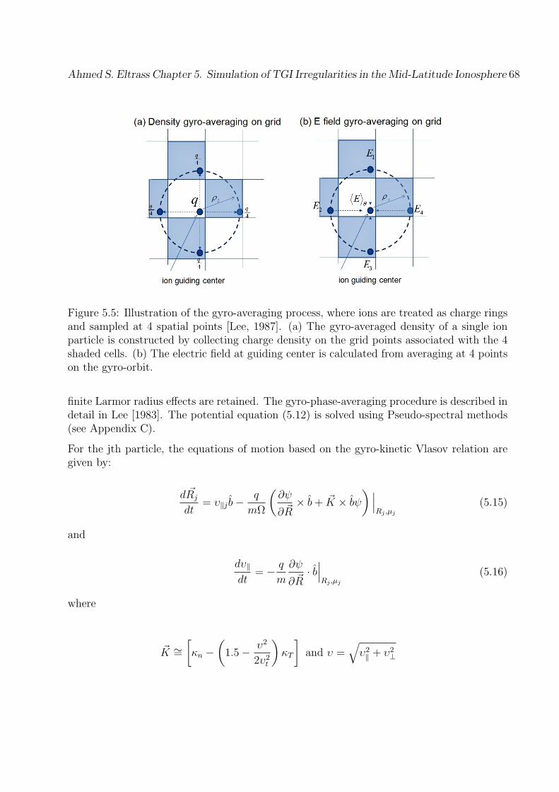
Ahmed S. Eltrass Chapter 5. Simulation of TGI Irregularities in the Mid-Latitude Ionosphere 68
Figure 5.5: Illustration of the gyro-averaging process, where ions are treated as charge ringsand sampled at 4 spatial points [Lee, 1987]. (a) The gyro-averaged density of a single ionparticle is constructed by collecting charge density on the grid points associated with the 4shaded cells. (b) The electric field at guiding center is calculated from averaging at 4 pointson the gyro-orbit.
finite Larmor radius effects are retained. The gyro-phase-averaging procedure is described indetail in Lee [1983]. The potential equation (5.12) is solved using Pseudo-spectral methods(see Appendix C).
For the jth particle, the equations of motion based on the gyro-kinetic Vlasov relation aregiven by:
dRj
dt= υ∥j b−
q
mΩ
(∂ψ
∂R× b+ K × bψ
) ∣∣∣Rj ,µj
(5.15)
and
dυ∥dt
= − q
m
∂ψ
∂R· b∣∣∣Rj ,µj
(5.16)
where
K ∼=[κn −
(1.5− υ2
2υ2t
)κT
]and υ =
√υ2∥ + υ2⊥
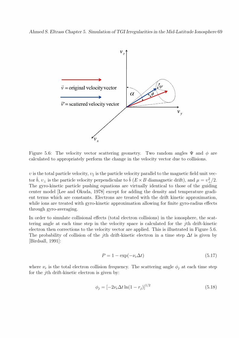
Ahmed S. Eltrass Chapter 5. Simulation of TGI Irregularities in the Mid-Latitude Ionosphere 69
Figure 5.6: The velocity vector scattering geometry. Two random angles Ψ and ϕ arecalculated to appropriately perform the change in the velocity vector due to collisions.
υ is the total particle velocity, υ∥ is the particle velocity parallel to the magnetic field unit vec-
tor b, υ⊥ is the particle velocity perpendicular to b (E×B diamagnetic drift), and µ = υ2⊥/2.The gyro-kinetic particle pushing equations are virtually identical to those of the guidingcenter model [Lee and Okuda, 1978] except for adding the density and temperature gradi-ent terms which are constants. Electrons are treated with the drift kinetic approximation,while ions are treated with gyro-kinetic approximation allowing for finite gyro-radius effectsthrough gyro-averaging.
In order to simulate collisional effects (total electron collisions) in the ionosphere, the scat-tering angle at each time step in the velocity space is calculated for the jth drift-kineticelectron then corrections to the velocity vector are applied. This is illustrated in Figure 5.6.The probability of collision of the jth drift-kinetic electron in a time step ∆t is given by[Birdsall, 1991]:
P = 1− exp(−νe∆t) (5.17)
where νe is the total electron collision frequency. The scattering angle ϕj at each time stepfor the jth drift-kinetic electron is given by:
ϕj = [−2νe∆t ln(1− rj)]1/2 (5.18)
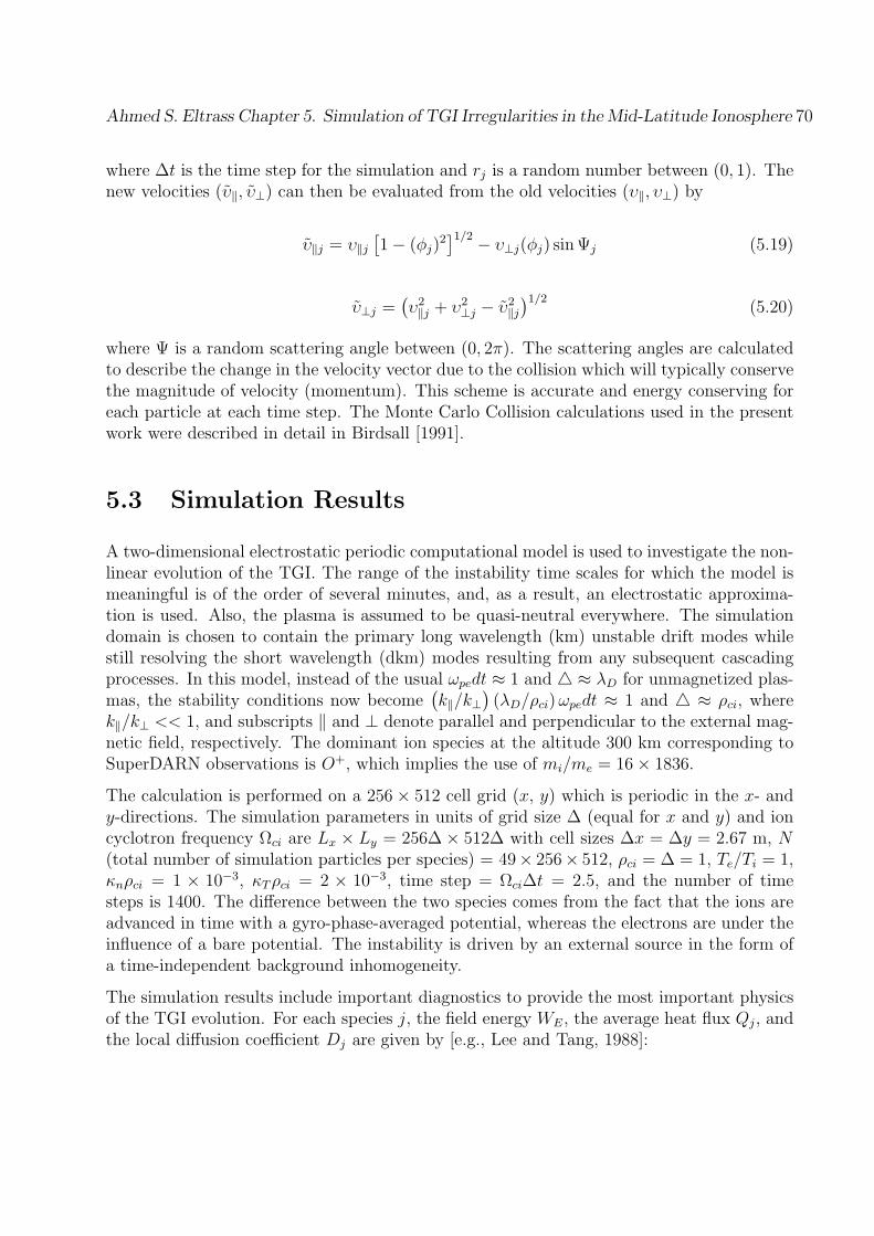
Ahmed S. Eltrass Chapter 5. Simulation of TGI Irregularities in the Mid-Latitude Ionosphere 70
where ∆t is the time step for the simulation and rj is a random number between (0, 1). Thenew velocities (υ∥, υ⊥) can then be evaluated from the old velocities (υ∥, υ⊥) by
υ∥j = υ∥j[1− (ϕj)
2]1/2 − υ⊥j(ϕj) sinΨj (5.19)
υ⊥j =(υ2∥j + υ2⊥j − υ2∥j
)1/2(5.20)
where Ψ is a random scattering angle between (0, 2π). The scattering angles are calculatedto describe the change in the velocity vector due to the collision which will typically conservethe magnitude of velocity (momentum). This scheme is accurate and energy conserving foreach particle at each time step. The Monte Carlo Collision calculations used in the presentwork were described in detail in Birdsall [1991].
5.3 Simulation Results
A two-dimensional electrostatic periodic computational model is used to investigate the non-linear evolution of the TGI. The range of the instability time scales for which the model ismeaningful is of the order of several minutes, and, as a result, an electrostatic approxima-tion is used. Also, the plasma is assumed to be quasi-neutral everywhere. The simulationdomain is chosen to contain the primary long wavelength (km) unstable drift modes whilestill resolving the short wavelength (dkm) modes resulting from any subsequent cascadingprocesses. In this model, instead of the usual ωpedt ≈ 1 and ≈ λD for unmagnetized plas-mas, the stability conditions now become
(k∥/k⊥
)(λD/ρci)ωpedt ≈ 1 and ≈ ρci, where
k∥/k⊥ << 1, and subscripts ∥ and ⊥ denote parallel and perpendicular to the external mag-netic field, respectively. The dominant ion species at the altitude 300 km corresponding toSuperDARN observations is O+, which implies the use of mi/me = 16× 1836.
The calculation is performed on a 256× 512 cell grid (x, y) which is periodic in the x- andy-directions. The simulation parameters in units of grid size ∆ (equal for x and y) and ioncyclotron frequency Ωci are Lx × Ly = 256∆ × 512∆ with cell sizes ∆x = ∆y = 2.67 m, N(total number of simulation particles per species) = 49× 256× 512, ρci = ∆ = 1, Te/Ti = 1,κnρci = 1 × 10⁻³, κTρci = 2 × 10⁻³, time step = Ωci∆t = 2.5, and the number of timesteps is 1400. The difference between the two species comes from the fact that the ions areadvanced in time with a gyro-phase-averaged potential, whereas the electrons are under theinfluence of a bare potential. The instability is driven by an external source in the form ofa time-independent background inhomogeneity.
The simulation results include important diagnostics to provide the most important physicsof the TGI evolution. For each species j, the field energy WE, the average heat flux Qj, andthe local diffusion coefficient Dj are given by [e.g., Lee and Tang, 1988]:

Ahmed S. Eltrass Chapter 5. Simulation of TGI Irregularities in the Mid-Latitude Ionosphere 71
0 200 400 600 800 1000 1200 1400
10−6
10−4
10−2
WEκ ne2
/(ω
* B)2
Electrostatic Field Energy
Ωcit
νe/Ω
ce=0
νe/Ω
ce= 3.4*10−5
νe/Ω
ce=9.1*10−5
Saturation
LinearGrowth
Figure 5.7: The normalized electrostatic field energy for three TGI simulations with varyingelectron collision frequency.
WE =∑i,j
| Ei,j |2 (5.21)
Qj =N∑j=1
(υ∥/υtj
)2υEj
N(5.22)
Dj =1
κn
N∑j=1
υEj
N(5.23)
where Ei,j is the grid electric field, υEjis the E × B drift (guiding center drift for each
particle), υ∥ is the parallel drift velocity, and N is the total number of particles in thesimulation. Note that the y-component of υEj
is used for calculating equations (5.22) and(5.23).
As shown in Figure 5.7, the TGI instability exhibits two distinct stages of development,i.e., the linear growth stage that fits the predictions of linear theory in Chapter 3 and thenonlinear oscillations associated with saturation. Three TGI simulations with the gyro-kinetic model, which have normalized electron collision frequency of νe/Ωce = 0.0, 3.4 ×10⁻⁵, and 9.1 × 10⁻⁵, were performed. Figure 5.7 shows the normalized field energy forthe three cases. With the introduction of collisions, the TGI instability grows faster andthe saturation amplitude scales by a factor of ∼ √
νe without exceeding an upper boundqΦ/kBTe ≈ (ω/Ωci)/(k⊥ρci)
2. This result has consistencies with previous work focused on
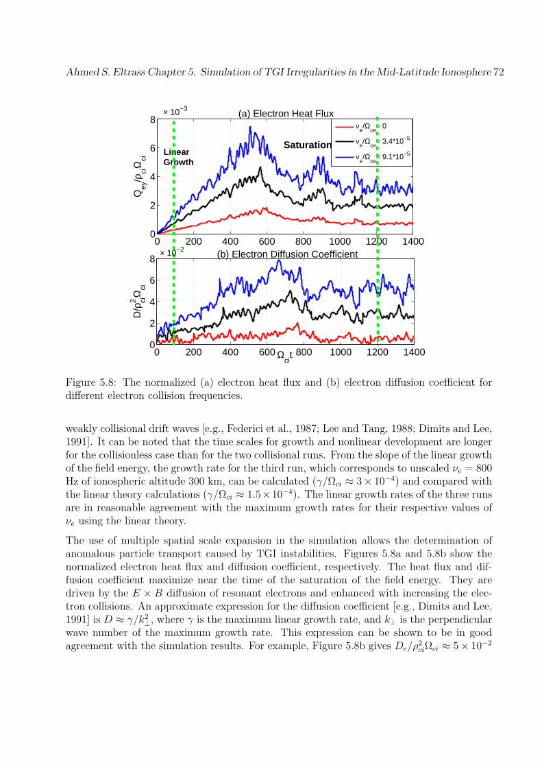
Ahmed S. Eltrass Chapter 5. Simulation of TGI Irregularities in the Mid-Latitude Ionosphere 72
0 200 400 600 800 1000 1200 14000
2
4
6
8
Qey
/ρciΩ
ci
(a) Electron Heat Flux
0 200 400 600 800 1000 1200 14000
2
4
6
8
Ωcit
D/ρ
ci2Ω
ci
(b) Electron Diffusion Coefficient
νe/Ω
ce= 0
νe/Ω
ce= 3.4*10−5
νe/Ω
ce= 9.1*10−5Linear
Growth
Saturation
× 10−3
× 10−2
Figure 5.8: The normalized (a) electron heat flux and (b) electron diffusion coefficient fordifferent electron collision frequencies.
weakly collisional drift waves [e.g., Federici et al., 1987; Lee and Tang, 1988; Dimits and Lee,1991]. It can be noted that the time scales for growth and nonlinear development are longerfor the collisionless case than for the two collisional runs. From the slope of the linear growthof the field energy, the growth rate for the third run, which corresponds to unscaled νe = 800Hz of ionospheric altitude 300 km, can be calculated (γ/Ωci ≈ 3× 10⁻⁴) and compared withthe linear theory calculations (γ/Ωci ≈ 1.5×10⁻⁴). The linear growth rates of the three runsare in reasonable agreement with the maximum growth rates for their respective values ofνe using the linear theory.
The use of multiple spatial scale expansion in the simulation allows the determination ofanomalous particle transport caused by TGI instabilities. Figures 5.8a and 5.8b show thenormalized electron heat flux and diffusion coefficient, respectively. The heat flux and dif-fusion coefficient maximize near the time of the saturation of the field energy. They aredriven by the E × B diffusion of resonant electrons and enhanced with increasing the elec-tron collisions. An approximate expression for the diffusion coefficient [e.g., Dimits and Lee,1991] is D ≈ γ/k2⊥, where γ is the maximum linear growth rate, and k⊥ is the perpendicularwave number of the maximum growth rate. This expression can be shown to be in goodagreement with the simulation results. For example, Figure 5.8b gives De/ρ
2ciΩci ≈ 5× 10⁻²

Ahmed S. Eltrass Chapter 5. Simulation of TGI Irregularities in the Mid-Latitude Ionosphere 73
x/ρci
y/ρ ci
(a) The Normalized Electron Density at Ωcit=100
50 100 150 200 250
50
100
150
200
250
300
350
400
450
500
ne /n
e (t=0)
0.8
0.9
1
1.1
TGIPhaseFronts
kxρ
ci
k yρ ci
(b) 2−D Wavenumber Spectrum at Ωcit=100
0.05 0.15 0.25 0.35 0.45 0.55 0.65 0.75 0.85 0.95
0.05
0.1
|qΦ/k
B Te | 2
0
10
20
30
40
50
Linear TGIMode
km−scale
Figure 5.9: Two-dimensional snapshots at t = 100/Ωci of (a) normalized electron densityand (b) electric potential wave number spectrum in the linear growth stage. In (a), theTGI waves propagate in the x-direction. In (b), the wave number spectrum shows the TGIkm-scale irregularities.
for νe/Ωce = 9.1× 10⁻⁵, whereas the approximate formula gives De/ρ2ciΩci ≈ 6× 10⁻². Since
periodic boundary conditions are imposed for the waves, the diffusion coefficient is ambipolar(Di ≈ De) in the simulation [Lee and Tang, 1988]. The particle diffusion is shown in Figure5.2 to be along the density gradient direction and opposite to the temperature gradient.
Focusing on the third run νe/Ωce = 9.1 × 10⁻⁵, which is most applicable for SuperDARNobservations at altitude 300 km, periodic snapshots of the electron density and the wavenumber spectrum were investigated to consider the density irregularities in detail. Thenormalized electron density snapshot during the linear growth stage shown in Figure 5.9aillustrates the formation of the TGI wave fronts. The TGI waves propagate in the x-directionwith phase velocity vph ≡ ω/kx. The phase velocity of these waves (∼ 3× 10⁻² m/s) lies inthe range predicted by linear theory which is the diamagnetic drift velocity. As discussedin Eltrass et al. [2014a], the diamagnetic drift velocity is typically too small relative tothe E ×B drift for SuperDARN radar measurement. The wave number spectrum snapshotshown in Figure 5.9b illustrates the km-scale TGI irregularities in the linear growth stage.The initial simulation mode growth corresponds to k⊥ρci ≈ 0.06 in Figure 5.9b which is tobe compared to k⊥ρci ≈ 0.08 from linear theory which is in reasonable agreement.
In the saturation stage, the formation of nonlinearly enhanced density regions is shown inFigure 5.10a. These nonlinearly generated fluctuations are responsible for the saturation ofthe instability. The TGI saturation is associated with the emergence of radially extendedstreamers with propagation velocity of vpr ≃ 0.1vph, where vph is the phase velocity in the x-
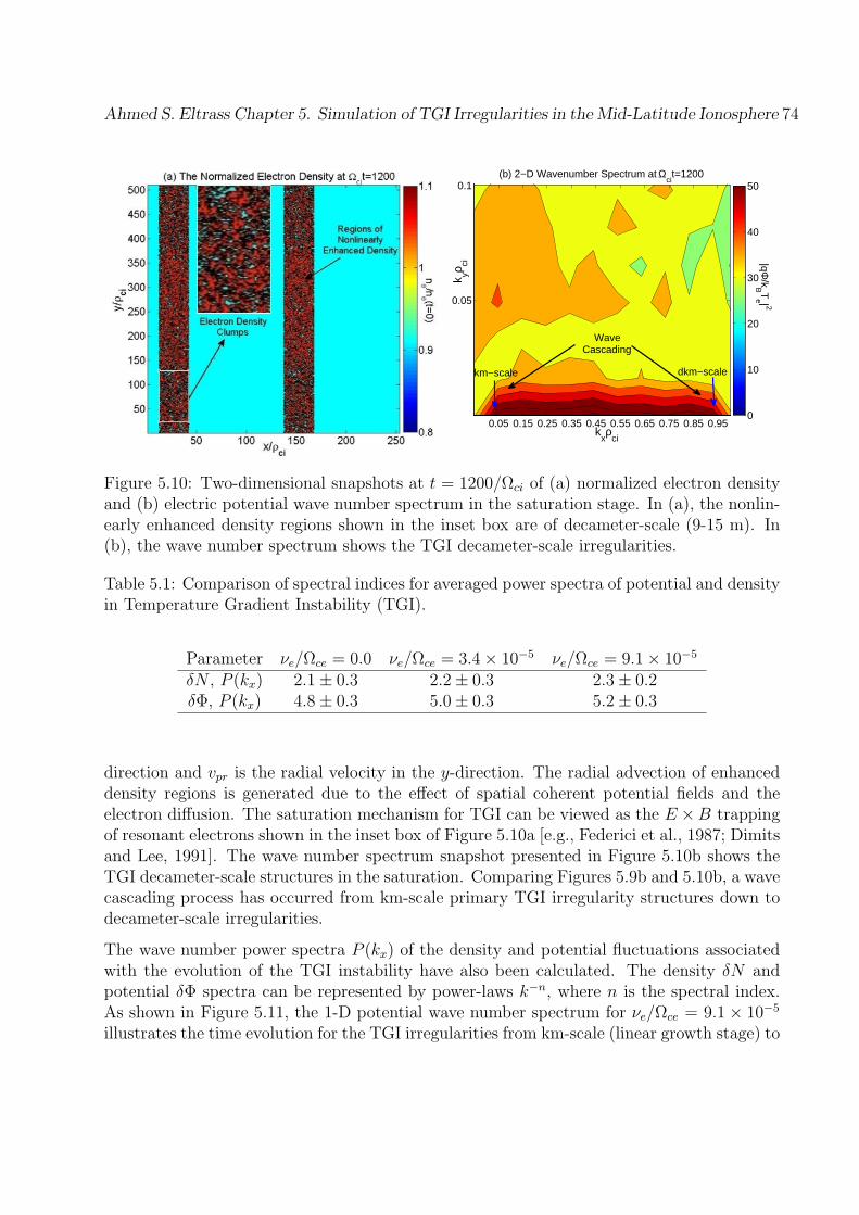
Ahmed S. Eltrass Chapter 5. Simulation of TGI Irregularities in the Mid-Latitude Ionosphere 74
kxρ
ci
k yρ ci
(b) 2−D Wavenumber Spectrum at Ωcit=1200
0.05 0.15 0.25 0.35 0.45 0.55 0.65 0.75 0.85 0.95
0.05
0.1
|qΦ/k
B Te | 2
0
10
20
30
40
50
WaveCascading
km−scale dkm−scale
Figure 5.10: Two-dimensional snapshots at t = 1200/Ωci of (a) normalized electron densityand (b) electric potential wave number spectrum in the saturation stage. In (a), the nonlin-early enhanced density regions shown in the inset box are of decameter-scale (9-15 m). In(b), the wave number spectrum shows the TGI decameter-scale irregularities.
Table 5.1: Comparison of spectral indices for averaged power spectra of potential and densityin Temperature Gradient Instability (TGI).
Parameter νe/Ωce = 0.0 νe/Ωce = 3.4× 10⁻⁵ νe/Ωce = 9.1× 10⁻⁵
δN , P (kx) 2.1± 0.3 2.2± 0.3 2.3± 0.2δΦ, P (kx) 4.8± 0.3 5.0± 0.3 5.2± 0.3
direction and vpr is the radial velocity in the y-direction. The radial advection of enhanceddensity regions is generated due to the effect of spatial coherent potential fields and theelectron diffusion. The saturation mechanism for TGI can be viewed as the E ×B trappingof resonant electrons shown in the inset box of Figure 5.10a [e.g., Federici et al., 1987; Dimitsand Lee, 1991]. The wave number spectrum snapshot presented in Figure 5.10b shows theTGI decameter-scale structures in the saturation. Comparing Figures 5.9b and 5.10b, a wavecascading process has occurred from km-scale primary TGI irregularity structures down todecameter-scale irregularities.
The wave number power spectra P (kx) of the density and potential fluctuations associatedwith the evolution of the TGI instability have also been calculated. The density δN andpotential δΦ spectra can be represented by power-laws k−n, where n is the spectral index.As shown in Figure 5.11, the 1-D potential wave number spectrum for νe/Ωce = 9.1× 10⁻⁵
illustrates the time evolution for the TGI irregularities from km-scale (linear growth stage) to

Ahmed S. Eltrass Chapter 5. Simulation of TGI Irregularities in the Mid-Latitude Ionosphere 75
10−2
10−1
100
100
101
102
103
104
105
Kxρ
ci
P(k
x)
Potential Wave Spectrum
Ωcit=100
Ωcit= 600
Ωcit= 1200
K−5.2
LinearMode
decameterscale
kmscale
Figure 5.11: The time evolution of the 1-D potential wave number spectrum, where P (kx)is the spatial power spectra averaged over the x-directions in arbitrary units. The spectralindex of k−5.2 is calculated from the linear slope of potential wave spectrum.
decameter-scale (saturation stage). For the potential wave spectrum, we find P (kx) ∝ k−nxx ,
nx = 5.2 ± 0.3, while for the density fluctuations, we find P (kx) ∝ k−nxx , nx = 2.3 ± 0.2.
The power spectra for the other two cases, i.e., νe/Ωce = 0.0 and 3.4 × 10⁻⁵, are displayedin Table 5.1. In general, the spectral indices for the density and potential are slightlysteeper for the more collisional case (νe/Ωce = 9.1 × 10⁻⁵) than for the other two cases.These computed spectral indices of TGI are comparable with other known instabilities,which cause irregularities in the F-region ionosphere, such as the Gradient Drift Instability(GDI) [Keskinen and Huba, 1990] and Kelvin-Helmholtz instability [Keskinen et al., 1988].The power spectra calculations suggest that the TGI wave cascading may contribute to theobserved SuperDARN irregularities at mid-latitudes [ Greenwald et al., 2006; de Larquier etal., 2014; Eltrass et al., 2014a, b].
Ahmed S. Eltrass Chapter 5. Simulation of TGI Irregularities in the Mid-Latitude Ionosphere 76
5.4 Discussion
The present work has demonstrated the usefulness of gyro-kinetic particle simulation as acomputational tool for studying the TGI decameter-scale irregularities in the F-region iono-sphere, where the plasma is collisional and drift instabilities are thought to be active. Thegyro-kinetic model used in this study contains the nonlinearities corresponding to F-regionirregularities. The model equations can be solved in their entirety via particle simulationwithout making prior judgments concerning the relative importance of each of the nonlin-ear terms. This is the first attempt to study the nonlinear evolution of the TGI in themid-latitude ionosphere, which provides meaningful correlations between the experimentalobservations of Chapter 4 and the theoretical results of Chapter 3.
The simulation results show that the TGI saturation amplitude is greatly enhanced bycollisions and appears to be rapidly approaching an upper bound as a function of ∼ √
νe.The saturation occurs due to the coherent radial advection of regions of nonlinearly enhanceddensity. This particle bunching, due to E×B trapping, is the cause of the electron-drift-wave-induced diffusion. The resonant particles play an important role in the TGI growth, as theyinteract with the TGI wave and contribute to the instability. However, as the amplitude ofthe wave increases, the resonant particles start to move relative to the wave in nearly circulartrajectories, causing the electrons to be E × B trapped [Federici et al., 1987]. The E × Btrapping of resonant electrons leads the wave-particle resonance process to be inhibited andsaturation occurs. Also, this E × B trapping inhibits further growth of the wave for thecollisionless case. Nevertheless, a stronger E×B trapping is required for the collisional caseto overcome the destabilizing effects of the collisions [e.g., Dimits and Lee, 1991]. This iswhy the saturation amplitude is increased with collisions as shown in Figure 5.7. Also, theelectron collisions play the same role in enhancing the heat flux and the diffusion coefficient,as they make more electrons lie in the nonlinearly broadened resonance.
The SuperDARN radar observations are in the decameter-scale regime which is of the orderof the ion gyro-radius (ρci ≈ 3 m). The development of the gyro-kinetic approach, whichextends into the kinetic regime, allows the investigation of the TGI as the cause for theseradar irregularities. The simulation results show that the scale size of the nonlinear electrondensity clumps (globs) during the TGI saturation stage are on the order of ∼ 3−5ρci, whichcorresponds to 9-15 meters. This suggests that the particle bunching shown in the insetbox of Figure 5.10a may be responsible for the decameter-scale irregularities observed bythe SuperDARN radars. This result reveals that these irregularities may occur due to thecoherent advection of regions of nonlinearly enhanced electron density. This implies thatthe TGI irregularities may be of km-scale (or longer) in the linear growth (long wavelength)and a cascade process occurs from km-scale irregularity structures down to the observeddecameter-scale irregularities as would be observed by the SuperDARN radars.
The mid-latitude decameter-scale ionospheric irregularities due to TGI are generally observedon the nightside. The absence of these irregularities during the day may occur due to the high
Ahmed S. Eltrass Chapter 5. Simulation of TGI Irregularities in the Mid-Latitude Ionosphere 77
E-region conductivity, which shorts out any electrostatic fields generated by the TGI in theF-region [e.g., Vickrey and Kelley, 1982]. The role of the E-region in shorting out F-regionelectrostatic fields during the day raises the importance of knowing the wavelength of theseirregularities. The irregularities with scale sizes smaller than 1 km are greatly attenuatedwhen mapped from the F- to the E-region [e.g., Farley, 1959; Kelley, 2009]. This impliesthat for the E-region to be responsible for shorting out the F-region TGI electric fields beforeand around sunset, the irregularities should be in the km-scale. This result agrees with thesimulation calculations, which suggest that a turbulent cascade process occurs from km-scaleprimary TGI irregularity structures down to the decameter-scale irregularities.
The spatial power spectra of the electrostatic potential and density fluctuations associatedwith the TGI are computed and found to be P (kx) ∝ k−5.2±0.3
x and P (kx) ∝ k−2.3±0.2x , re-
spectively. The spectra calculations of TGI lie in the same range of the previous numericalsimulations of GDI [e.g., Keskinen, 1984; Keskinen and Huba, 1990; Guzdar et al., 1998],showing that the spectral indices of TGI and GDI density irregularities are of the order 2.An interpretation of the spectral analysis is that TGI and GDI irregularities are initially gen-erated at kilometer-scale, become unstable and dissipate their energy by generating smallersized (decameter-scale) irregularities, known as turbulent cascade processes. Note that thegrowth times for the disturbed mid-latitude irregularities are on the order of several min-utes [e.g., Mishin and Blaunstein, 2008; Keskinen et al., 2004], which is consistent with theTGI and GDI simulation results. This suggests that ionospheric density, electric field, andelectron temperature irregularities can be driven in the mid-latitude ionosphere from theTGI in association with the GDI. The experimental observations along with simulation re-sults suggest that turbulent cascade processes of both TGI and GDI may be responsible forthe decameter-scale irregularities that occur under disturbed conditions of the mid-latitudeF-region ionosphere.
Chapter 6
Potential Impact of Mid-LatitudeIrregularities on GPS Signals
6.1 Introduction
This chapter provides an overview of the Global Navigation Satellite System (GNSS), theionospheric effects on GPS signals, and the radio wave propagation through ionosphericirregularities relevant to this investigation. In this chapter, the potential impact of themid-latitude ionospheric irregularities on GPS signals is investigated utilizing modeling andobservations. The disturbed-time mid-latitude ionospheric irregularities presented in Chap-ter 4 are sufficiently strong to cause amplitude and phase scintillations for GPS signals.Also, the computational results in Chapter 5 suggest that these ionospheric irregularities areof km-scale (or longer) and a cascade process occurs from km-scale irregularity structuresdown to the observed decameter-scale irregularities. This raises the importance of analyzingmultiple GPS data sets at mid-latitudes to investigate the conclusions that turbulent cascadeprocesses of both TGI and GDI are responsible for the mid-latitude GPS scintillations. TheGPS measurements along with simulation results of Chapter 5 are investigated to obtainthe spectral characteristics of irregularities producing ionospheric scintillations. Both GPSspectral measurements and simulation results are compared with previous in-situ satellitemeasurements during disturbed periods at mid-latitudes.
6.1.1 Global Navigation Satellite System (GNSS)
Global Navigation Satellite System (GNSS) is a satellite navigation system with global cov-erage. It includes constellations of Earth-orbiting satellites that broadcast their locations inspace and time. GNSS systems have revolutionized both the defense and consumer productindustries and their applications have become ubiquitous in today’s society. In the near
78
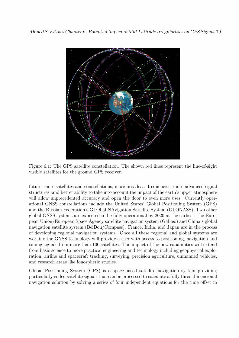
Ahmed S. Eltrass Chapter 6. Potential Impact of Mid-Latitude Irregularities on GPS Signals 79
Figure 6.1: The GPS satellite constellation. The shown red lines represent the line-of-sightvisible satellites for the ground GPS receiver.
future, more satellites and constellations, more broadcast frequencies, more advanced signalstructures, and better ability to take into account the impact of the earth’s upper atmospherewill allow unprecedented accuracy and open the door to even more uses. Currently oper-ational GNSS constellations include the United States’ Global Positioning System (GPS)and the Russian Federation’s GLObal NAvigation Satellite System (GLONASS). Two otherglobal GNSS systems are expected to be fully operational by 2020 at the earliest: the Euro-pean Union/European Space Agency satellite navigation system (Galileo) and China’s globalnavigation satellite system (BeiDou/Compass). France, India, and Japan are in the processof developing regional navigation systems. Once all these regional and global systems areworking the GNSS technology will provide a user with access to positioning, navigation andtiming signals from more than 100 satellites. The impact of the new capabilities will extendfrom basic science to more practical engineering and technology including geophysical explo-ration, airline and spacecraft tracking, surveying, precision agriculture, unmanned vehicles,and research areas like ionospheric studies.
Global Positioning System (GPS) is a space-based satellite navigation system providingparticularly coded satellite signals that can be processed to calculate a fully three-dimensionalnavigation solution by solving a series of four independent equations for the time offset in
Ahmed S. Eltrass Chapter 6. Potential Impact of Mid-Latitude Irregularities on GPS Signals 80
the receiver clock and their three position coordinates [Hofmann-Wellenhof et al., 2001].The GPS constellation is composed of 24 to 32 medium Earth-orbit satellites in six differentorbital planes with an inclination of around 55 [e.g., Hofmann-Wellenhof et al., 2001]. Thespacecraft orbits are located 26,600 km from the center of the Earth and designed to have atleast six satellites line-of-sight from almost everywhere on Earth’s surface (see Figure 6.1).All satellites broadcast their ephemeris and timing information at the same two frequencies:L1 (1575.42 MHz) and L2 (1227.6 MHz). Satellite signals are encoded using Code DivisionMultiple Access (CDMA) spread-spectrum technique, allowing messages from individualsatellites to be distinguished from each other based on a high-rate Pseudo-Random Noise(PRN) code unique to each satellite. The L1 carrier is modulated by both the coarse-acquisition (C/A) code and the encrypted precise (P(Y)) code, while the L2 carrier is onlymodulated by the P(Y) code [Hofmann-Wellenhof et al., 2001]. Most civilian receivers onlyuse the L1 C/A code signal which gives accuracies of 5-15 m. Military receivers use the P(Y)code on both L1 and L2, yielding accuracies of 3-5 m. The GPS dual frequency receivers (L1and L2) provide the ability to measure the dispersive properties of the refractive ionospherethat can be used to remove ionospheric errors and to feed assimilative ionospheric models[e.g., Hajj et al., 2004; Coster et al., 2005]. Due to the huge applications of GPS technology,a modernization process is underway satellites to provide more benefits for both militaryand civilian users.
6.1.2 Ionospheric Effects on GPS Signals
The ionosphere represents one of the largest source of positioning error for the GPS appli-cations. The electron density dependent refractive index of the ionosphere produces rangeerrors and range rate errors for GPS signals. This results from the change in optical pathlength caused by the Total Electron Content (TEC) of the intervening ionosphere [Klobuchar,1996]. The TEC is defined as the total number of free electrons in a rectangular solid witha one-square-meter cross section along a path between the receiver and the satellite. Figure6.2 illustrates the propagation delays introduced on GPS signals by the ionospheric TEC.Note that the product of the phase velocity and the group velocity of GPS signals is equalto the square of speed of light, i.e., υgυp = c2. So, the higher TEC slows down the groupvelocity and speeds up the phase velocity to keep their product a constant. A faster phasevelocity produces unexpected phase shifts that challenge the tracking loops in GPS receivers’phase lock loops, while a slower group velocity causes ranging errors. For an undisturbedionosphere, these are the only effects that impact the performance of GPS signals. However,the GPS signals can be perturbed by electron density fluctuations in the ionosphere thatmay cause fluctuations in the received signal characteristics, known as scintillations [Crane,1977; Gwal et al., 2004].
Ionospheric scintillation is characterized by rapid variations in the amplitude and phase ofthe radio signals due to variations in the local index of refraction along the propagation path.The ionospheric irregularities producing GPS scintillations are predominantly at altitudes
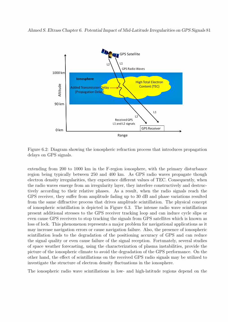
Ahmed S. Eltrass Chapter 6. Potential Impact of Mid-Latitude Irregularities on GPS Signals 81
Figure 6.2: Diagram showing the ionospheric refraction process that introduces propagationdelays on GPS signals.
extending from 200 to 1000 km in the F-region ionosphere, with the primary disturbanceregion being typically between 250 and 400 km. As GPS radio waves propagate thoughelectron density irregularities, they experience different values of TEC. Consequently, whenthe radio waves emerge from an irregularity layer, they interfere constructively and destruc-tively according to their relative phases. As a result, when the radio signals reach theGPS receiver, they suffer from amplitude fading up to 30 dB and phase variations resultedfrom the same diffractive process that drives amplitude scintillation. The physical conceptof ionospheric scintillation is depicted in Figure 6.3. The intense radio wave scintillationspresent additional stresses to the GPS receiver tracking loop and can induce cycle slips oreven cause GPS receivers to stop tracking the signals from GPS satellites which is known asloss of lock. This phenomenon represents a major problem for navigational applications as itmay increase navigation errors or cause navigation failure. Also, the presence of ionosphericscintillation leads to the degradation of the positioning accuracy of GPS and can reducethe signal quality or even cause failure of the signal reception. Fortunately, several studiesof space weather forecasting, using the characterization of plasma instabilities, provide thepicture of the ionospheric climate to avoid the degradation of the GPS performance. On theother hand, the effect of scintillations on the received GPS radio signals may be utilized toinvestigate the structure of electron density fluctuations in the ionosphere.
The ionospheric radio wave scintillations in low- and high-latitude regions depend on the
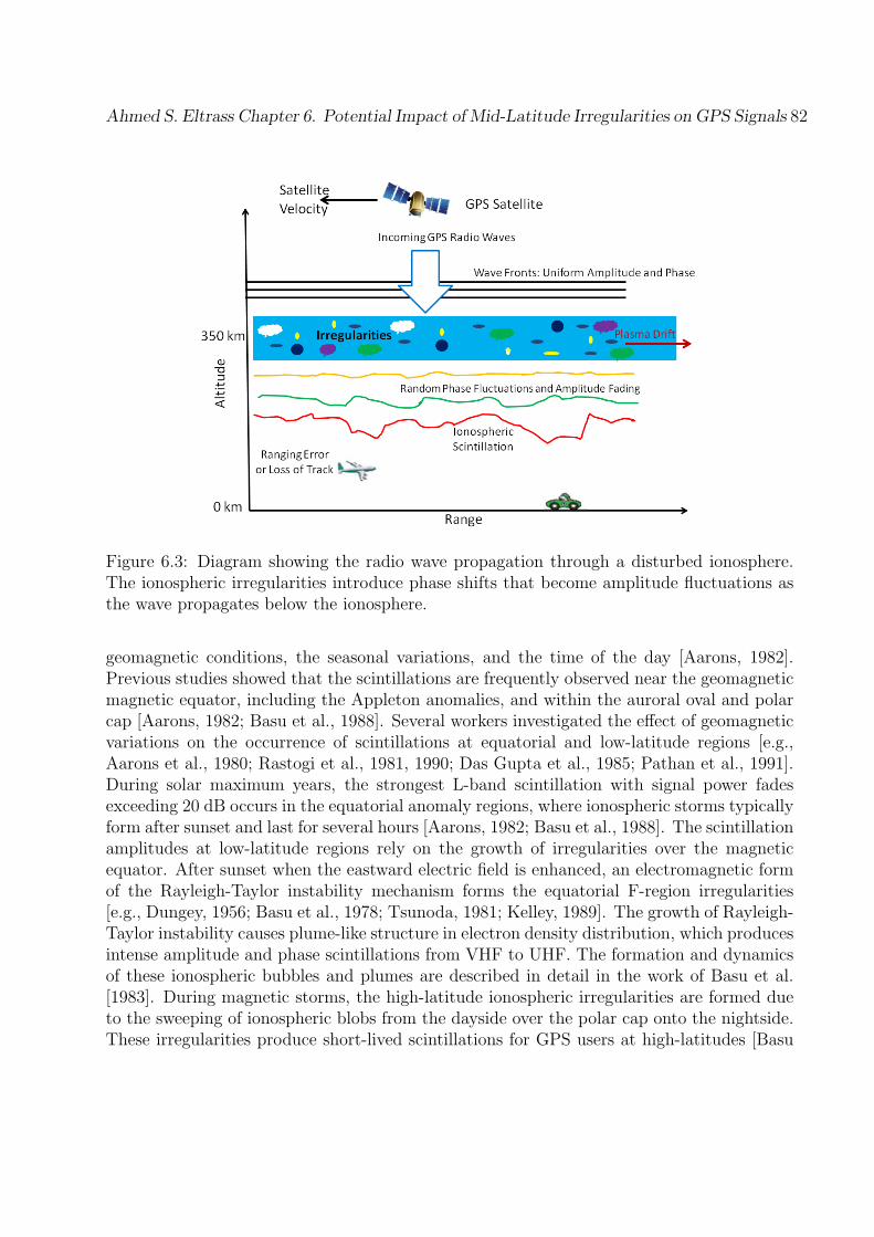
Ahmed S. Eltrass Chapter 6. Potential Impact of Mid-Latitude Irregularities on GPS Signals 82
Figure 6.3: Diagram showing the radio wave propagation through a disturbed ionosphere.The ionospheric irregularities introduce phase shifts that become amplitude fluctuations asthe wave propagates below the ionosphere.
geomagnetic conditions, the seasonal variations, and the time of the day [Aarons, 1982].Previous studies showed that the scintillations are frequently observed near the geomagneticmagnetic equator, including the Appleton anomalies, and within the auroral oval and polarcap [Aarons, 1982; Basu et al., 1988]. Several workers investigated the effect of geomagneticvariations on the occurrence of scintillations at equatorial and low-latitude regions [e.g.,Aarons et al., 1980; Rastogi et al., 1981, 1990; Das Gupta et al., 1985; Pathan et al., 1991].During solar maximum years, the strongest L-band scintillation with signal power fadesexceeding 20 dB occurs in the equatorial anomaly regions, where ionospheric storms typicallyform after sunset and last for several hours [Aarons, 1982; Basu et al., 1988]. The scintillationamplitudes at low-latitude regions rely on the growth of irregularities over the magneticequator. After sunset when the eastward electric field is enhanced, an electromagnetic formof the Rayleigh-Taylor instability mechanism forms the equatorial F-region irregularities[e.g., Dungey, 1956; Basu et al., 1978; Tsunoda, 1981; Kelley, 1989]. The growth of Rayleigh-Taylor instability causes plume-like structure in electron density distribution, which producesintense amplitude and phase scintillations from VHF to UHF. The formation and dynamicsof these ionospheric bubbles and plumes are described in detail in the work of Basu et al.[1983]. During magnetic storms, the high-latitude ionospheric irregularities are formed dueto the sweeping of ionospheric blobs from the dayside over the polar cap onto the nightside.These irregularities produce short-lived scintillations for GPS users at high-latitudes [Basu

Ahmed S. Eltrass Chapter 6. Potential Impact of Mid-Latitude Irregularities on GPS Signals 83
et al., 2002]. Smith et al. [2008] showed that individual auroral arcs can cause diffractivefading of GPS signals due to the E-region precipitation. Coster et al. [2005] investigatedthe GPS scintillations in the auroral and polar cap regions by the aid of GPS Total ElectronContent (TEC) mapping. Several studies showed the predominance of phase scintillations athigh-latitudes than amplitude scintillations [e.g., Mitchell et al., 2005; Kinrade et al., 2012].
The equatorial and high-latitude ionospheric irregularities have been studied in detail formany decades to investigate their influence on GPS signals. On the other hand, the mid-latitude ionospheric scintillation is still largely unexplored due to lack of models and obser-vations that can explain the characteristics of mid-latitude scintillations. In the context ofthis chapter, we restrict our interest to the potential impact of mid-latitude irregularitieson GPS scintillations. The radar observations in Chapter 4 in conjunction with simulationresults in Chapter 5 suggest that turbulent cascade processes of both TGI and GDI may beresponsible for the disturbed-time irregularities that cause GPS scintillations. This needsto be verified by analyzing GPS data sets at mid-latitudes to monitor the amplitude andphase scintillations and to obtain the spectral characteristics of irregularities producing GPSscintillations.
6.2 Wave Propagation through Ionospheric Irregular-
ities
Several previous studies provided thorough information regarding the wave propagationthrough an irregularity layer [e.g., Tatarskii, 1971; Yeh and Liu, 1982]. We will outlinethe concept of the one-dimensional weak scattering of radio waves by ionospheric irregular-ities. Assuming that the irregularities have scale sizes much larger than the incident radiowave’s wavelength and that the variations in permittivity along the ray path are small, thescalar Helmholtz wave equation can be used to model the radio wave propagation throughan irregular scattering medium [e.g., Yeh and Liu, 1982]. The Helmholtz wave equation isgiven by:
∇2A+ k2[1 + ϵ1(´r)
]A = 0 (6.1)
where A is the electric field amplitude, k is the wave number of the incident radio signal,ϵ1 is the deviation from free space permittivity, r is the distance from the irregularities tothe receiver, and ´r is the location of the irregularities. Assuming the incident signal is aplane wave, and the irregularities have wavelengths much larger than the Fresnel radius(rF =
√2λr), the solution for the Helmholtz wave equation is [Beach, 1998]:
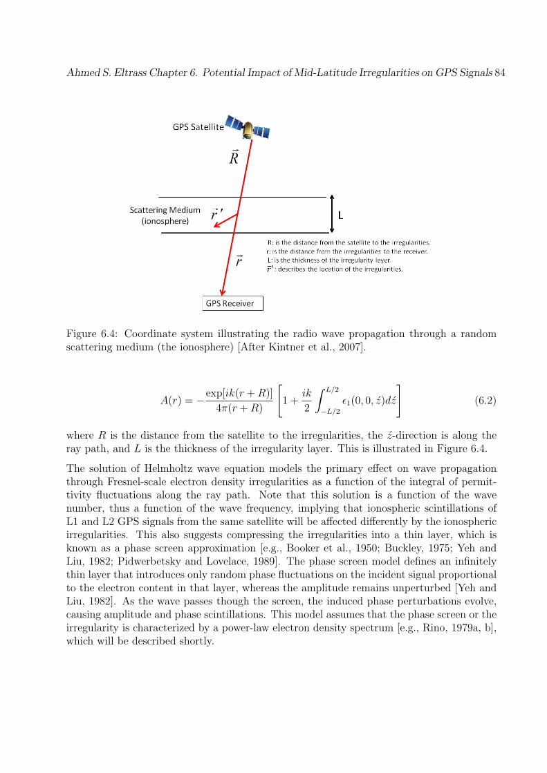
Ahmed S. Eltrass Chapter 6. Potential Impact of Mid-Latitude Irregularities on GPS Signals 84
Figure 6.4: Coordinate system illustrating the radio wave propagation through a randomscattering medium (the ionosphere) [After Kintner et al., 2007].
A(r) = −exp[ik(r +R)]
4π(r +R)
[1 +
ik
2
∫ L/2
−L/2
ϵ1(0, 0, z)dz
](6.2)
where R is the distance from the satellite to the irregularities, the z-direction is along theray path, and L is the thickness of the irregularity layer. This is illustrated in Figure 6.4.
The solution of Helmholtz wave equation models the primary effect on wave propagationthrough Fresnel-scale electron density irregularities as a function of the integral of permit-tivity fluctuations along the ray path. Note that this solution is a function of the wavenumber, thus a function of the wave frequency, implying that ionospheric scintillations ofL1 and L2 GPS signals from the same satellite will be affected differently by the ionosphericirregularities. This also suggests compressing the irregularities into a thin layer, which isknown as a phase screen approximation [e.g., Booker et al., 1950; Buckley, 1975; Yeh andLiu, 1982; Pidwerbetsky and Lovelace, 1989]. The phase screen model defines an infinitelythin layer that introduces only random phase fluctuations on the incident signal proportionalto the electron content in that layer, whereas the amplitude remains unperturbed [Yeh andLiu, 1982]. As the wave passes though the screen, the induced phase perturbations evolve,causing amplitude and phase scintillations. This model assumes that the phase screen or theirregularity is characterized by a power-law electron density spectrum [e.g., Rino, 1979a, b],which will be described shortly.
Ahmed S. Eltrass Chapter 6. Potential Impact of Mid-Latitude Irregularities on GPS Signals 85
The intensity of the observed scintillation is typically quantified by a metric called theamplitude scintillation index S4. The S4 index is defined as the ratio of the standard deviationof the received signal power to the average signal power computed over a period of time[Briggs and Parkin, 1963]:
S4 =
√⟨I2⟩ − ⟨I⟩2
⟨I⟩2(6.3)
where I is the signal intensity (amplitude squared), and the angular brackets represent en-semble time averaging, commonly taken over a 60 second interval. The averaging time periodcould be arbitrarily larger or smaller than 60 second, however, it must be long comparedto the Fresnel length (rF ) divided by the irregularity drift speed [e.g., Kintner et al., 2007].The S4 index may be interpreted as the fractional fluctuation of the signal (i.e., S4 = 0.0indicates no scintillation, whereas S4 = 1.0 indicates saturation).
Phase scintillations are primarily produced by ionospheric density fluctuations at small wavenumbers near the first Fresnel radius (rF/
√2 ). The former quantity (small wave numbers)
is produced by the TEC changes along the wave path, while the latter quantity (near thefirst Fresnel radius) is caused by the interference between different phases exiting the thindiffractive layer [ Kintner et al., 2007]. The phase deviation of the GPS signal producedduring transit of the ionosphere is given by:
ϕ =40.3
cfTEC (6.4)
where ϕ is the signal phase deviation, TEC =∫nedρ is the total electron content, f is the
signal frequency, and c is the speed of light.
Phase scintillation monitoring is usually measured by means of the standard deviation of ϕin radians, known as the sigma-phi (σϕ) index. The σϕ index is sensitive to how the phasemeasurements are detrended, which may admit receiver clock noise or GPS satellite motion[e.g., Forte and Radicella, 2002; Forte, 2005; Beach, 2006]. The detrended phase data areused to estimate important spectral parameters such as the strength of the phase PowerSpectral Density (PSD) and the associated spectral index [e.g., Rino, 1979a, b; Rufenach,1972].
6.3 GPS Scintillations at Mid-Latitudes
The mid-latitude ionospheric region is assumed to be a less active scintillation environmentand is considered to be absent of L-band GPS scintillations. This general claim results from
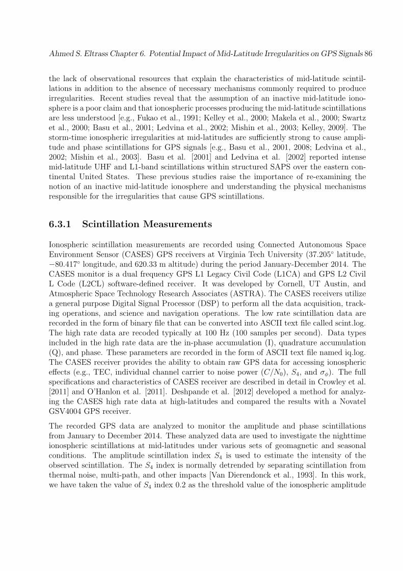
Ahmed S. Eltrass Chapter 6. Potential Impact of Mid-Latitude Irregularities on GPS Signals 86
the lack of observational resources that explain the characteristics of mid-latitude scintil-lations in addition to the absence of necessary mechanisms commonly required to produceirregularities. Recent studies reveal that the assumption of an inactive mid-latitude iono-sphere is a poor claim and that ionospheric processes producing the mid-latitude scintillationsare less understood [e.g., Fukao et al., 1991; Kelley et al., 2000; Makela et al., 2000; Swartzet al., 2000; Basu et al., 2001; Ledvina et al., 2002; Mishin et al., 2003; Kelley, 2009]. Thestorm-time ionospheric irregularities at mid-latitudes are sufficiently strong to cause ampli-tude and phase scintillations for GPS signals [e.g., Basu et al., 2001, 2008; Ledvina et al.,2002; Mishin et al., 2003]. Basu et al. [2001] and Ledvina et al. [2002] reported intensemid-latitude UHF and L1-band scintillations within structured SAPS over the eastern con-tinental United States. These previous studies raise the importance of re-examining thenotion of an inactive mid-latitude ionosphere and understanding the physical mechanismsresponsible for the irregularities that cause GPS scintillations.
6.3.1 Scintillation Measurements
Ionospheric scintillation measurements are recorded using Connected Autonomous SpaceEnvironment Sensor (CASES) GPS receivers at Virginia Tech University (37.205 latitude,−80.417 longitude, and 620.33 m altitude) during the period January-December 2014. TheCASES monitor is a dual frequency GPS L1 Legacy Civil Code (L1CA) and GPS L2 CivilL Code (L2CL) software-defined receiver. It was developed by Cornell, UT Austin, andAtmospheric Space Technology Research Associates (ASTRA). The CASES receivers utilizea general purpose Digital Signal Processor (DSP) to perform all the data acquisition, track-ing operations, and science and navigation operations. The low rate scintillation data arerecorded in the form of binary file that can be converted into ASCII text file called scint.log.The high rate data are recoded typically at 100 Hz (100 samples per second). Data typesincluded in the high rate data are the in-phase accumulation (I), quadrature accumulation(Q), and phase. These parameters are recorded in the form of ASCII text file named iq.log.The CASES receiver provides the ability to obtain raw GPS data for accessing ionosphericeffects (e.g., TEC, individual channel carrier to noise power (C/N0), S4, and σϕ). The fullspecifications and characteristics of CASES receiver are described in detail in Crowley et al.[2011] and O’Hanlon et al. [2011]. Deshpande et al. [2012] developed a method for analyz-ing the CASES high rate data at high-latitudes and compared the results with a NovatelGSV4004 GPS receiver.
The recorded GPS data are analyzed to monitor the amplitude and phase scintillationsfrom January to December 2014. These analyzed data are used to investigate the nighttimeionospheric scintillations at mid-latitudes under various sets of geomagnetic and seasonalconditions. The amplitude scintillation index S4 is used to estimate the intensity of theobserved scintillation. The S4 index is normally detrended by separating scintillation fromthermal noise, multi-path, and other impacts [Van Dierendonck et al., 1993]. In this work,we have taken the value of S4 index 0.2 as the threshold value of the ionospheric amplitude
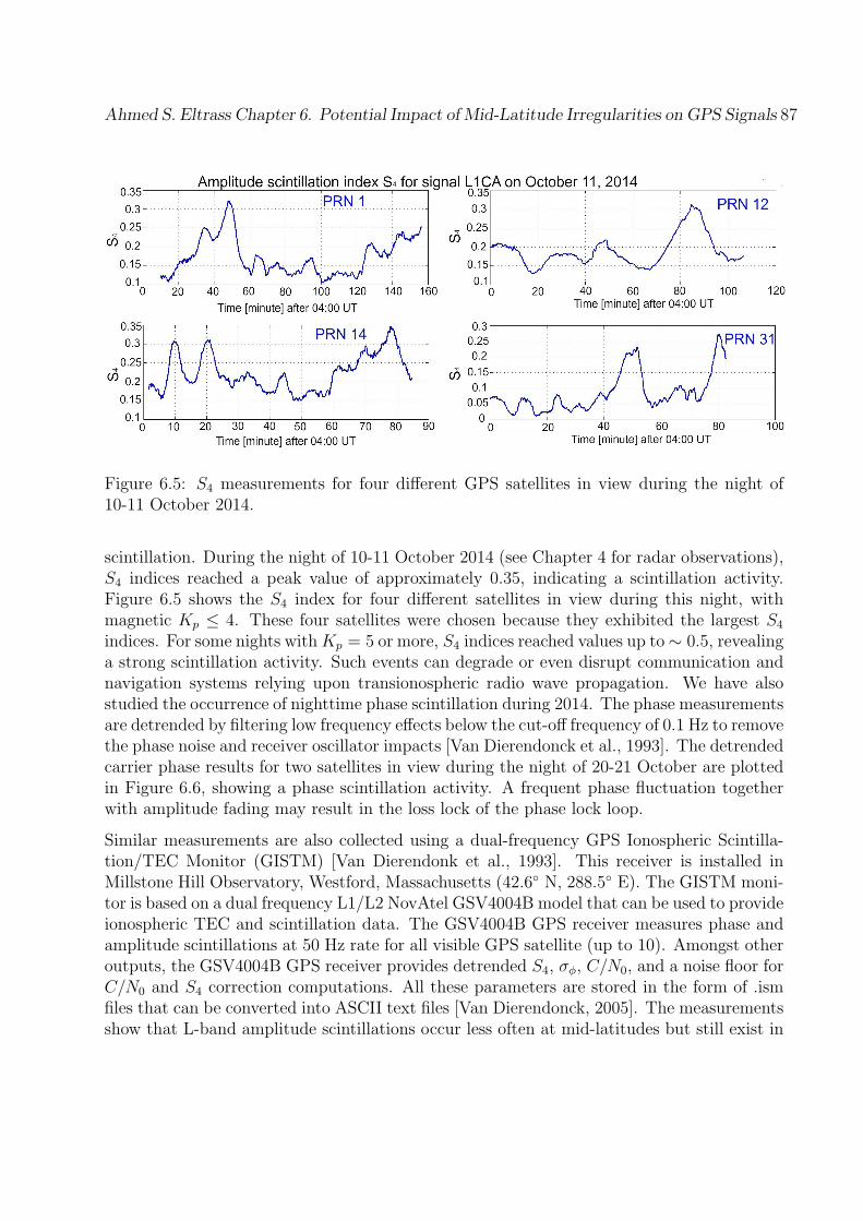
Ahmed S. Eltrass Chapter 6. Potential Impact of Mid-Latitude Irregularities on GPS Signals 87
Figure 6.5: S4 measurements for four different GPS satellites in view during the night of10-11 October 2014.
scintillation. During the night of 10-11 October 2014 (see Chapter 4 for radar observations),S4 indices reached a peak value of approximately 0.35, indicating a scintillation activity.Figure 6.5 shows the S4 index for four different satellites in view during this night, withmagnetic Kp ≤ 4. These four satellites were chosen because they exhibited the largest S4
indices. For some nights withKp = 5 or more, S4 indices reached values up to∼ 0.5, revealinga strong scintillation activity. Such events can degrade or even disrupt communication andnavigation systems relying upon transionospheric radio wave propagation. We have alsostudied the occurrence of nighttime phase scintillation during 2014. The phase measurementsare detrended by filtering low frequency effects below the cut-off frequency of 0.1 Hz to removethe phase noise and receiver oscillator impacts [Van Dierendonck et al., 1993]. The detrendedcarrier phase results for two satellites in view during the night of 20-21 October are plottedin Figure 6.6, showing a phase scintillation activity. A frequent phase fluctuation togetherwith amplitude fading may result in the loss lock of the phase lock loop.
Similar measurements are also collected using a dual-frequency GPS Ionospheric Scintilla-tion/TEC Monitor (GISTM) [Van Dierendonk et al., 1993]. This receiver is installed inMillstone Hill Observatory, Westford, Massachusetts (42.6 N, 288.5 E). The GISTM moni-tor is based on a dual frequency L1/L2 NovAtel GSV4004B model that can be used to provideionospheric TEC and scintillation data. The GSV4004B GPS receiver measures phase andamplitude scintillations at 50 Hz rate for all visible GPS satellite (up to 10). Amongst otheroutputs, the GSV4004B GPS receiver provides detrended S4, σϕ, C/N0, and a noise floor forC/N0 and S4 correction computations. All these parameters are stored in the form of .ismfiles that can be converted into ASCII text files [Van Dierendonck, 2005]. The measurementsshow that L-band amplitude scintillations occur less often at mid-latitudes but still exist in
Ahmed S. Eltrass Chapter 6. Potential Impact of Mid-Latitude Irregularities on GPS Signals 88
Figure 6.6: Phase scintillation measurements for two different GPS satellites in view duringthe night of 20-21 October 2014.
association with magnetic storms.
6.3.2 Amplitude Scintillation Analysis
The first observations of strong mid-latitude GPS scintillations at latitudes corresponding tothe northeastern United States were measured on 25-26 September 2001 [Basu et al., 2001;Ledvina et al., 2002]. These intense amplitude scintillations (S4 ≈ 0.8) occurred during themain phase of a moderate geomagnetic storm (Dst = −100 nT) when a Storm-EnhancedDensity (SED) event coupled with a broad and structured ionospheric trough occurred overthe eastern United States [e.g., Erickson et al., 2002; Ledvina et al., 2002]. Several studiessuggested that these scintillations were created in regions of large ionospheric velocities,and associated with fast ionospheric drifts in Sub-Auroral Polarization Streams (SAPS)[e.g., Foster and Vo, 2002; Ledvina et al., 2004; Foster et al., 2004]. Other occurrencesof mid-latitude GPS scintillations were reported in Japan during magnetic storms over a2-year period [e.g., Kintner et al., 2007]. These scintillation events were associated withTraveling Ionospheric Disturbances (TIDs) of large-scale structures (100 km). The L-bandscintillations may be related to the large drift velocities and associated velocity shear at mid-latitudes. Also, the L-band scintillations exist on or near steep electron density gradients,
Ahmed S. Eltrass Chapter 6. Potential Impact of Mid-Latitude Irregularities on GPS Signals 89
implying that a process that produces ionospheric irregularities is required to cause GPSscintillations. The sharp ionospheric temperature and density gradients during magneticstorms derive various plasma instability processes that cause GPS signals to scintillate. Allthe aforementioned observations reveal less understood ionospheric physical mechanisms thatexist at mid-latitudes and that cause irregularities leading to ionospheric GPS scintillations.
We have studied the occurrence of nighttime ionospheric scintillation using data from GPSstations at mid-latitudes during the period January-December 2014. The results show weakto moderate amplitude scintillations of GPS L1 signals occurring at mid-latitudes in thepresence of ionospheric irregularities during disturbed geomagnetic conditions. In order forGPS scintillations to occur, a wave must pass through ionospheric structures on the order ofthe Fresnel radius. This reveals that large-scale ionospheric irregularities, roughly 350-400m, are required to cause a GPS wave’s amplitude to fluctuate at some observation point onthe ground. This is one reason for GPS scintillations being not frequent at mid-latitudesbut common at the equatorial anomalies, where large plasma irregularities are generatedby spread F drifts. In this study, the scintillation results along with radar observations inChapter 4 suggest that the observed decameter-scale irregularities that cause SuperDARNbackscatter, co-exist with kilometer-scale irregularities that cause L-band scintillations. Theresults also reveal that mid-latitude scintillations are more common than previously thought,however, intense scintillations may be so exacting that only rare occurrences are possible.The reasonable agreement between experimental and computational results suggests thatturbulent cascade processes of both TGI and GDI are responsible for the disturbed-timeirregularities that cause GPS scintillations. Further insight could be obtained by analyzingmultiple data sets from fast sampling GPS receivers at mid-latitudes.
6.4 Spectral Measurements of Density Irregularities at
Mid-Latitudes
As the radio signals pass through ionospheric irregularities, the spatial pattern of varyingintensity is converted into temporal fluctuations or scintillations that can be recorded bythe ground GPS receiver. Parameters such as the strength of density fluctuations and ir-regularities in the power spectrum can be used to study the distribution of the spatial scalelengths in the ground scintillation pattern. The phase scintillation spectrum on ground canbe expressed as [Rino, 1979a]:
Sϕ(f) =T
(f 20 + f 2)
p/2(6.5)
where T is the spectral strength of the PSD at 1 Hz, f0 is the outer scale frequency whichcorresponds to the maximum irregularity size, and p is the ground spectral index. The

Ahmed S. Eltrass Chapter 6. Potential Impact of Mid-Latitude Irregularities on GPS Signals 90
spectral index of a power spectrum p is the magnitude of the spectral slope that can beobtained by a linear fit between the upper and lower cut-off frequencies on a log-log scale.The in-situ irregularity spectral index n can be related to the ground spectral index p byn = p− 1 [e.g., Bhattacharyya and Rastogi, 1985, 1991; Rino et al., 1981; Basu et al., 1983].When f >> f0, the phase PSD can be expressed as:
Sϕ(f) = Tf−p (6.6)
The amplitude scintillation spectrum follows the same relationship, however, it is attenuatedafter a cut-off frequency, known as the Fresnel frequency. Note that the radio wave must passthrough ionospheric structures on the order of the Fresnel radius to experience amplitudescintillation. The Fresnel radius gets translated into the Fresnel frequency for the amplitudescintillation power spectrum. The Fresnel frequency is given by:
fF =VrelrF
=Vrel√2λr
(6.7)
where fF is the Fresnel frequency, Vrel is the relative velocity between the satellite andthe irregularity, λ is the wavelength, and r is the distance from the irregularities to thereceiver. Note that the signal fluctuations caused by ionospheric irregularities are inverselyproportional to the frequency of the incident signal. Yeh and Liu [1982] showed that thelonger Fresnel length of the lower frequency signals corresponds to larger power spectraldensities within the irregularities, implying that lower frequency signals are greatly influencedby irregularities than higher frequency signals.
Several theoretical and experimental studies have shown that the spectra of electron densityfluctuations and the associated amplitude and phase scintillation spectra follow a power-lawbetween an inner and an outer scale size [e.g., Rumsey, 1975; Rino, 1979a, b; Rufenach,1972]. Wernik et al. [1997] reported that the spectra of electron density fluctuations obeythe power-law quite well at high frequencies for weak scintillation and that spectrum appearsto be Gaussian rather than a power-law for strong scintillation. For irregularities followinga power-law spectrum, the plot of spectral power in dB versus log frequency should bea straight line for frequencies in excess of the Fresnel frequency, while the spectral powerin dB versus frequency squared for Gaussian irregularities should be a straight line abovethe Fresnel frequency [e.g., Singleton, 1974; Banola et al., 2005]. Strangeways [2009] andStrangeways et al. [2011] showed that the ground spectral parameters can be estimated fromthe observed amplitude and phase scintillations (S4 and σϕ) when high sample rate data arenot readily available. Several workers investigated the relation between the ground spectralindex and the irregularity intensity [e.g., Rino et al., 1981; Livingston et al., 1981; Werniket al., 2007; Conker et al., 2003; Aquino et al., 2007].
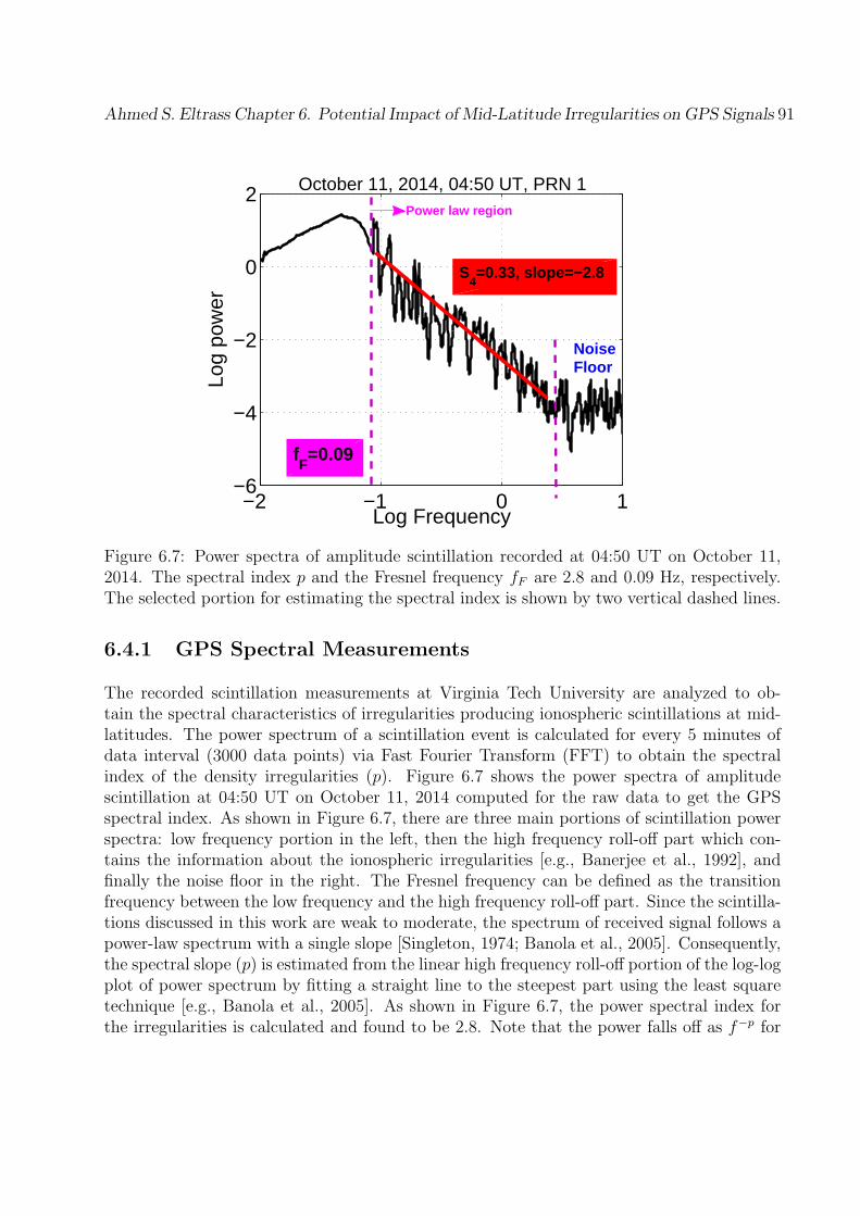
Ahmed S. Eltrass Chapter 6. Potential Impact of Mid-Latitude Irregularities on GPS Signals 91
−2 −1 0 1−6
−4
−2
0
2
Log Frequency
Log
pow
er
October 11, 2014, 04:50 UT, PRN 1Power law region
fF=0.09
NoiseFloor
S4=0.33, slope=−2.8
Figure 6.7: Power spectra of amplitude scintillation recorded at 04:50 UT on October 11,2014. The spectral index p and the Fresnel frequency fF are 2.8 and 0.09 Hz, respectively.The selected portion for estimating the spectral index is shown by two vertical dashed lines.
6.4.1 GPS Spectral Measurements
The recorded scintillation measurements at Virginia Tech University are analyzed to ob-tain the spectral characteristics of irregularities producing ionospheric scintillations at mid-latitudes. The power spectrum of a scintillation event is calculated for every 5 minutes ofdata interval (3000 data points) via Fast Fourier Transform (FFT) to obtain the spectralindex of the density irregularities (p). Figure 6.7 shows the power spectra of amplitudescintillation at 04:50 UT on October 11, 2014 computed for the raw data to get the GPSspectral index. As shown in Figure 6.7, there are three main portions of scintillation powerspectra: low frequency portion in the left, then the high frequency roll-off part which con-tains the information about the ionospheric irregularities [e.g., Banerjee et al., 1992], andfinally the noise floor in the right. The Fresnel frequency can be defined as the transitionfrequency between the low frequency and the high frequency roll-off part. Since the scintilla-tions discussed in this work are weak to moderate, the spectrum of received signal follows apower-law spectrum with a single slope [Singleton, 1974; Banola et al., 2005]. Consequently,the spectral slope (p) is estimated from the linear high frequency roll-off portion of the log-logplot of power spectrum by fitting a straight line to the steepest part using the least squaretechnique [e.g., Banola et al., 2005]. As shown in Figure 6.7, the power spectral index forthe irregularities is calculated and found to be 2.8. Note that the power falls off as f−p for
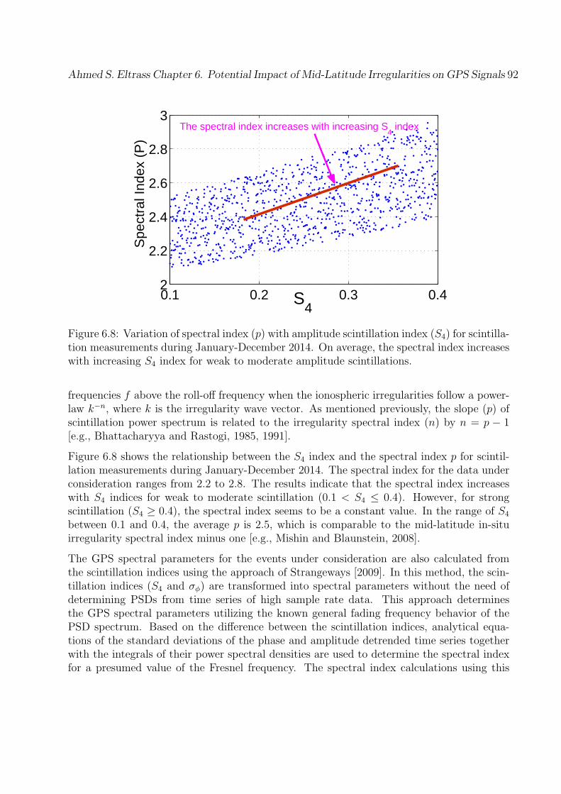
Ahmed S. Eltrass Chapter 6. Potential Impact of Mid-Latitude Irregularities on GPS Signals 92
0.1 0.2 0.3 0.42
2.2
2.4
2.6
2.8
3
S4
Spe
ctra
l Ind
ex (
P)
The spectral index increases with increasing S4 index
Figure 6.8: Variation of spectral index (p) with amplitude scintillation index (S4) for scintilla-tion measurements during January-December 2014. On average, the spectral index increaseswith increasing S4 index for weak to moderate amplitude scintillations.
frequencies f above the roll-off frequency when the ionospheric irregularities follow a power-law k−n, where k is the irregularity wave vector. As mentioned previously, the slope (p) ofscintillation power spectrum is related to the irregularity spectral index (n) by n = p − 1[e.g., Bhattacharyya and Rastogi, 1985, 1991].
Figure 6.8 shows the relationship between the S4 index and the spectral index p for scintil-lation measurements during January-December 2014. The spectral index for the data underconsideration ranges from 2.2 to 2.8. The results indicate that the spectral index increaseswith S4 indices for weak to moderate scintillation (0.1 < S4 ≤ 0.4). However, for strongscintillation (S4 ≥ 0.4), the spectral index seems to be a constant value. In the range of S4
between 0.1 and 0.4, the average p is 2.5, which is comparable to the mid-latitude in-situirregularity spectral index minus one [e.g., Mishin and Blaunstein, 2008].
The GPS spectral parameters for the events under consideration are also calculated fromthe scintillation indices using the approach of Strangeways [2009]. In this method, the scin-tillation indices (S4 and σϕ) are transformed into spectral parameters without the need ofdetermining PSDs from time series of high sample rate data. This approach determinesthe GPS spectral parameters utilizing the known general fading frequency behavior of thePSD spectrum. Based on the difference between the scintillation indices, analytical equa-tions of the standard deviations of the phase and amplitude detrended time series togetherwith the integrals of their power spectral densities are used to determine the spectral indexfor a presumed value of the Fresnel frequency. The spectral index calculations using this
Ahmed S. Eltrass Chapter 6. Potential Impact of Mid-Latitude Irregularities on GPS Signals 93
approximated method are in reasonable agreement with the high rate spectral results.
6.4.2 Satellite In-Situ Spectral Measurements
The satellite in-situ measurements of electron density fluctuations provide direct informationabout the structure of ionospheric irregularities that may cause scintillation of radio waves ontransionospheric links. Several previous studies utilized satellite passes over storm-time mid-latitude troughs from one or several polar orbiting satellites to investigate the characteristic ofSAPS events [e.g., Mishin et al., 2003; Wang et al., 2008, 2011, 2012; Henderson et al., 2010].The observations reveal rapidly fluctuating plasma drifts, magnetic fields, and ionosphericdensities associated with either structured SAPS or elevated electron temperature. TheDefense Meteorological Satellite Program (DMSP) F13 and 14 satellites, while flying nearthe regions of intense radio signal scintillations, detected mid-latitude small-scale density,electric field, velocity, and electron temperature structures during the magnetic storms ofSeptember 1999 and 2001. During these events, the geographic local times of the orbits areeither near the 1800-0600 (F13) or 2100-0900 (F14, F15) meridians. Each satellite carries asuite of sensors to measure the drift motions of ionospheric ions and electrons, the electrondensities and temperatures, and perturbations of the Earth’s magnetic field. The DMSPsatellite overflights indicated that the small-scale irregularities responsible for the intensemid-latitude UHF and L1-band scintillations were collocated with the SAPS-related densitytrough equatorward and poleward walls [e.g., Mishin et al., 2003; Basu et al., 2001], revealingthat regions of strongest irregularities and GPS scintillations are causally relayed.
Using DMSP satellite data, Mishin and Blaunstein [2008] calculated the power spectral den-sities of mid-latitude irregularities as a function of spatial wave number during scintillationintervals on 26 September 2001. They showed that the power spectra of the density irreg-ularities in the range of 10 > k ≥ 1 km−1 admit a power-law characterization k−n with aspectral index n ∼ 1.7− 2. As shown in Figure 6.9, the spatial wave number regime corre-sponding to spatial wavelengths between several hundred meters and several tens of metersis well-represented by a power-law, yielding a spectral index of 1.8. The data available to thisstudy are not sufficient to use in-situ satellite measurements and calculate the power spectraldensities for the events under investigation. However, the spectra simulations of TGI andGDI density irregularities [e.g., Eltrass and Scales, 2014; Keskinen and Huba, 1990] alongwith ground GPS measurements are in reasonable agreement with DMSP satellite measure-ments for previous disturbed-time events in the nightside sub-auroral ionosphere [e.g., Fosterand Rich, 1998; Mishin et al., 2003; Mishin and Blaunstein, 2008]. Also, the growth timesfor the disturbed mid-latitude irregularities are on the order of several minutes [e.g., Mishinand Blaunstein, 2008; Keskinen et al., 2004], which is consistent with the TGI and GDIsimulation results. An interpretation of the spectral analysis is that TGI and GDI irregular-ities are initially generated at kilometer-scale, become unstable and dissipate their energy bygenerating smaller sized (decameter-scale) irregularities. The in-situ satellite observationsalong with GPS measurements lend further support to the belief that turbulent cascade
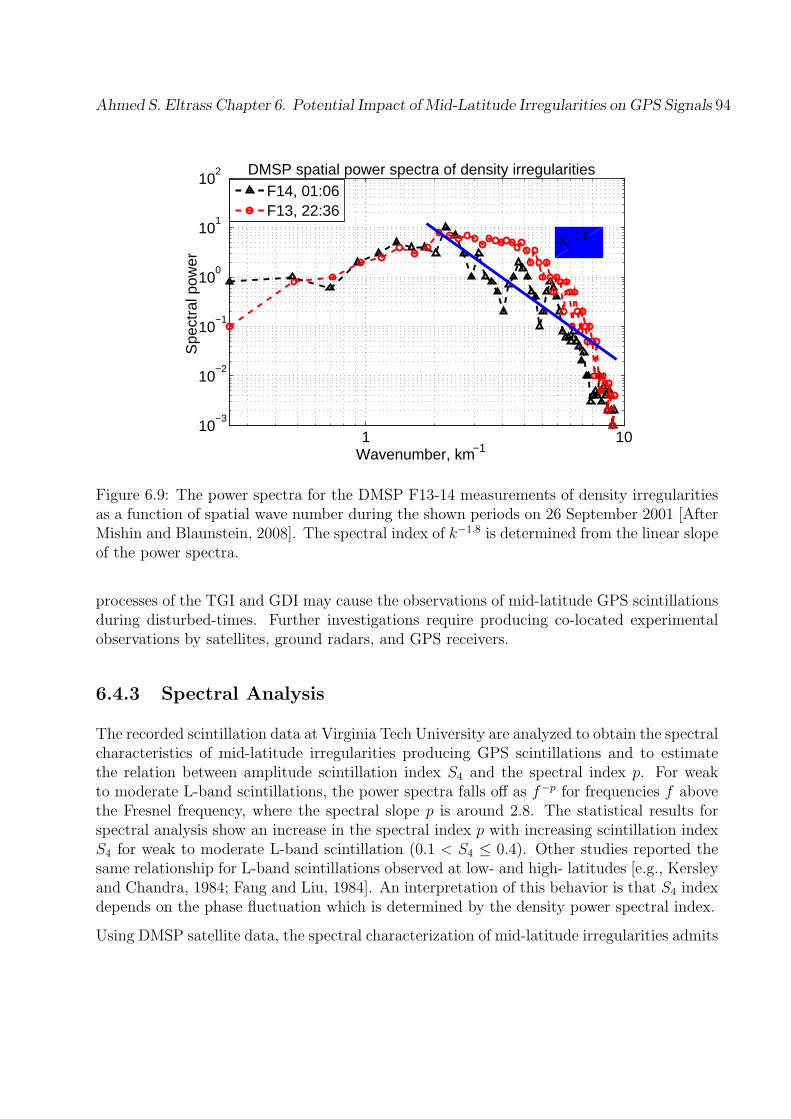
Ahmed S. Eltrass Chapter 6. Potential Impact of Mid-Latitude Irregularities on GPS Signals 94
1 1010
−3
10−2
10−1
100
101
102
Wavenumber, km−1
Spe
ctra
l pow
erDMSP spatial power spectra of density irregularities
F14, 01:06F13, 22:36
K−1.8
Figure 6.9: The power spectra for the DMSP F13-14 measurements of density irregularitiesas a function of spatial wave number during the shown periods on 26 September 2001 [AfterMishin and Blaunstein, 2008]. The spectral index of k−1.8 is determined from the linear slopeof the power spectra.
processes of the TGI and GDI may cause the observations of mid-latitude GPS scintillationsduring disturbed-times. Further investigations require producing co-located experimentalobservations by satellites, ground radars, and GPS receivers.
6.4.3 Spectral Analysis
The recorded scintillation data at Virginia Tech University are analyzed to obtain the spectralcharacteristics of mid-latitude irregularities producing GPS scintillations and to estimatethe relation between amplitude scintillation index S4 and the spectral index p. For weakto moderate L-band scintillations, the power spectra falls off as f−p for frequencies f abovethe Fresnel frequency, where the spectral slope p is around 2.8. The statistical results forspectral analysis show an increase in the spectral index p with increasing scintillation indexS4 for weak to moderate L-band scintillation (0.1 < S4 ≤ 0.4). Other studies reported thesame relationship for L-band scintillations observed at low- and high- latitudes [e.g., Kersleyand Chandra, 1984; Fang and Liu, 1984]. An interpretation of this behavior is that S4 indexdepends on the phase fluctuation which is determined by the density power spectral index.
Using DMSP satellite data, the spectral characterization of mid-latitude irregularities admits

Ahmed S. Eltrass Chapter 6. Potential Impact of Mid-Latitude Irregularities on GPS Signals 95
a single power-law with a spectral index of n ∼ 1.7 − 2 for scale sizes less than 1 km [e.g.,Foster and Rich, 1998; Mishin et al., 2003; Mishin and Blaunstein, 2008]. The ground spectralindices for the present study are shown to be between 2.2 and 2.8, where the mean value isaround 2.5 for weak to moderate GPS scintillations. The GPS spectral indices lie in the samerange of the numerical simulations of TGI and GDI, however, they are slightly different thanthose in the irregularity spectra (n = p− 1) because of the nonlinear transformations on thesignal propagating through the irregularity and space. Both simulation results and groundobservations are consistent with previous DMSP satellite measurements during magneticstorm periods [e.g., Foster and Rich, 1998; Mishin et al., 2003; Mishin and Blaunstein, 2008].In view of observed power-law variation of the irregularity spectrum, ionospheric structureson the order of the Fresnel radius (i.e., 350-400 m for L-band) will contribute mostly toamplitude scintillation, while irregularities of smaller-scales will introduce less amplitudefluctuations. The radar observations along with GPS measurements suggest that decameter-and large-scale irregularities may coexist under disturbed conditions of the mid-latitude F-region ionosphere. This also suggests that turbulent cascade processes of both TGI and GDImay be responsible for the disturbed-time irregularities that cause GPS scintillations.

Chapter 7
Conclusions and Future Work
7.1 Summary and Conclusions
The research presented in this dissertation focuses on modeling and analyzing the plasmawave irregularities at mid-latitudes through the coordination between SuperDARNHF radars,Incoherent Scatter Radars (ISRs), and GPS receivers under various sets of geomagnetic con-ditions. The potential impact of mid-latitude irregularities on GPS signals is investigatedutilizing modeling and observations.
In Chapter 3, the electrostatic dispersion relation for the Temperature Gradient Instability(TGI) has been extended into the kinetic regime appropriate for SuperDARN radar frequen-cies by including Landau damping, finite gyro-radius effects, and temperature anisotropy.The kinetic dispersion relation of TGI is solved and underscores limitations in fluid theory forshort wavelengths (decameter-scale waves). The variations of TGI growth rate with electroncollision frequency, temperature gradients, density gradients, and the angle between wavevector and magnetic field have been studied. The kinetic dispersion relation of the GDIwith finite ion gyro-radius effects has also been solved to consider decameter-scale wavesgeneration. The TGI and GDI calculations are obtained over a wide range of parameters toprovide perspective on the experimental observations in Chapter 4.
In Chapter 4, data from the Millstone Hill ISR and the Wallops SuperDARN radar havebeen analyzed to identify the plasma instability mechanisms responsible for the formation ofwidespread decameter-scale mid-latitude irregularities. Improving upon previous results ofGreenwald et al. [2006], the temperature and density gradients are calculated in the directionperpendicular to the geomagnetic field in the top-side F-region. A critical comparison of TGIand GDI is made for SuperDARN observations by studying the variation of TGI and GDIgrowth rates for both perpendicular and meridional gradients as a function of universal time.The growth rate calculations suggest that the TGI is the dominant plasma instability duringthe experiment, while the GDI does not play a significant role in the primary SAIS irregu-
96
Ahmed S. Eltrass Chapter 7. Conclusions and Future Work 97
larity generation. This result modifies previous conclusions of Greenwald et al. [2006] whichrelied on the dusk scatter associated with the GDI [Ruohoniemi et al., 1988] to explain theinitial observed irregularities after sunset. The TGI growth rates due to perpendicular andmeridional gradients are shown to be important, however, the perpendicular growth is moresignificant. The perpendicular TGI growth rate persists throughout the entire experimentand can explain the observed low-velocity SAIS. The absence of the observed irregularitiesbefore and around sunset is due to the high E-region conductivity, which leads to the sup-pression of irregularity growth. This is the first experimental confirmation that mid-latitudedecameter-scale ionospheric irregularities are produced by the TGI or by turbulent cascadefrom primary irregularity structures produced from this instability.
Chapter 4 has also investigated the TGI and GDI as the cause of mid-latitude decameter-scaleionospheric irregularities during disturbed geomagnetic conditions. Co-located experimentalobservations by the Blackstone SuperDARN radar and the Millstone Hill ISR are performedunder quiet and disturbed sets of geomagnetic conditions to identify what plasma instabilitymechanisms predominate. A time series for the growth rate of both TGI and GDI is de-veloped for these events, showing that the TGI is the most likely generation mechanism forquiet-time irregularities, while the TGI in association with the GDI or a cascade productfrom them may be responsible for the disturbed-time observations.
Chapter 5 has demonstrated the usefulness of gyro-kinetic particle simulation as a compu-tational tool for studying the TGI decameter-scale irregularities in the F-region ionosphere,where the plasma is collisional and drift instabilities are thought to be active. While lineartheory predicts the dominant wavelengths, it cannot fully describe the nonlinearly saturatedbehavior as observed by radars. The nonlinear evolution of the TGI is investigated utilizinggyro-kinetic Particle-In-Cell (PIC) simulation techniques with Monte Carlo collisions for thefirst time. The purpose of this investigation is to identify the mechanism responsible forthe nonlinear saturation as well as the associated anomalous transport. It is found thatthe saturation amplitude level and the associated diffusion are greatly enhanced as a resultof electron collisions. The simulation results indicate that the nonlinear E × B convection(trapping) of the electrons is the dominant TGI saturation mechanism. The spatial powerspectra of the electrostatic potential and density fluctuations associated with the TGI arealso computed and the results show wave cascading of TGI from kilometer scales into thedecameter-scale regime of the radar observations. The spectra calculations of TGI lie inthe same range of previous numerical simulations of GDI [e.g., Keskinen and Huba, 1990;Guzdar et al., 1998], showing that the spectral index of TGI and GDI density irregularitiesare of the order 2. An interpretation of the spectral analysis is that initially TGI or/andGDI irregularities are generated at large-scale size or sizes (km-scale) and the dissipationof the energy associated with these irregularities occurs by generating smaller and smaller(decameter-scale) irregularities. The TGI and GDI wave cascading confirm the assumptionthat the E-region may be responsible for shorting out the F-region TGI and GDI electricfields before and around sunset and ultimately leading to irregularity suppression.
In Chapter 6, we have investigated the influence of mid-latitude ionospheric irregularities on
Ahmed S. Eltrass Chapter 7. Conclusions and Future Work 98
the GPS signals by analyzing data from GPS receivers at mid-latitudes. These analyzed dataare used to study the amplitude and phase fluctuations of the GPS signals and to investigatethe spectral index variations due to ionospheric irregularities. The GPS measurements showweak to moderate scintillations of GPS L1 signals occurring at mid-latitudes in the presenceof ionospheric irregularities during disturbed geomagnetic conditions. The results show thatmid-latitude scintillations are more common than previously thought, however, intense scin-tillations may be so exacting that only rare occurrences are possible. The spectral indices ofthe spectra observed on the ground are comparable with the numerical simulations of TGIand GDI, however, they are slightly different than those in the irregularity spectra due tothe nonlinear transformations on the signal propagating through the irregularity and space.Both simulation results and ground observations are consistent with previous DMSP satellitemeasurements during magnetic storm periods in the nightside sub-auroral ionosphere [e.g.,Foster and Rich, 1998; Mishin et al., 2003; Mishin and Blaunstein, 2008]. The scintillationresults along with radar observations suggest that the observed decameter-scale irregularitiesthat cause SuperDARN backscatter, co-exist with kilometer-scale irregularities that cause L-band scintillations. The alignment between the experimental, theoretical, and computationalresults of this study lends further support to the belief that turbulent cascade processes ofTGI and GDI may cause the observations of GPS scintillations that occur under disturbedconditions of the mid-latitude F-region ionosphere.
7.2 Future Work
The results of the work presented in this dissertation bring to light a wide number of scientificand engineering research aspects as follows:
• The radar observations along with GPS measurements reveal that the claim of an in-active mid-latitude ionosphere is a poor assumption and that plasma instability processesproducing the mid-latitude irregularities are less understood. The alignment between exper-imental, theoretical, and computational results suggests that a TGI turbulent cascade maybe responsible for the observed quiet-time irregularities, while turbulent cascade processes ofboth TGI and GDI may cause the disturbed-time irregularities. Important aspects of thesemechanisms should be studied in further detail including different spatial scales, nonlinearcascading, and the impact of E-region conductance. This could be determined by produc-ing in-situ measurements of electric fields, densities and temperatures in the bottom- andtop-side F-region. Further investigations require the coordination between in-situ satellitemeasurements, ground radar observations, and GPS data under various sets of geomagneticand seasonal conditions.
• The GPS scintillation results imply that that large-scale ionospheric irregularities, at least350-400 m, should exist to cause the measured GPS L-band scintillations. The GPS measure-ments along with radar observations suggest that the observed decameter-scale irregularitiesthat cause SuperDARN backscatter, co-exist with kilometer-scale irregularities that cause
Ahmed S. Eltrass Chapter 7. Conclusions and Future Work 99
L-band scintillations. This needs to be further verified by observing these larger scale sizesvia in-situ satellite measurements and conducting a statistical analysis to characterize andexamine the existence of these large-scale irregularities. The GPS measurements also revealthat mid-latitude scintillations are more common than currently appreciated. Further in-sight could be obtained by analyzing multiple data sets from fast sampling GPS receivers,which are adequate to directly measure diffractive scintillations at mid-latitudes.
• All of the physics to model the storm-time ionospheric irregularities is not included in thecurrent simulation model [e.g., Mishin et al., 2003; Keskinen et al., 2004]. The disturbed F-region is characterized by rapidly fluctuating plasma drifts, magnetic fields, and ionosphericdensities associated with either structured SAPS or elevated electron temperature. Keskinenet al. [2004] developed a fluid model for the TGI and GDI small-scale structures in the storm-time mid-latitude SAPS-driven density trough ionosphere. The effects included in this modelare ring current precipitation, parallel currents, rapid sub-auroral ion drifts, temperatureand density gradients, and storm-induced neutral winds. The nonlinear evolution associatedwith these processes can be studied by developing gyro-kinetic plasma simulation models thatcontain the different effects relevant to the disturbed F-region irregularities. Also, developingcomputational models to study the relation between velocity shear, density gradients, andirregularity formation in the sub-auroral ionospheric trough should be the next step forresearch in this area.
• Another effort should be focused on studying the morphology and characteristics of thehigh-latitude irregularities resulted from the complex magnetosphere-ionosphere couplingmechanisms. Important aspects for the feasible mechanisms that cause irregularity genera-tion should be considered in detail including the nonlinear evolution using high performancecomputing techniques, and the potential impact on GNSS scintillations. The radio wave scin-tillations at high-latitudes are still less understood due to lack of models and observationsthat can explain the cause and distribution of the polar and auroral irregularities.
• As GPS is fully modernized and other GNSS satellite systems become operational, severalnew signals and codes will usher in a new era of ionospheric science. The GNSS low fre-quency signals will encounter more frequent and severe diffractive and refractive ionosphericscintillations than higher frequencies. For example, the use of GPS L5 signal (1176.45 MHz)will allow the investigation of GPS scintillations at longer Fresnel lengths (intense irregular-ities) in addition to the experience of more phase shift for the same density perturbation,compared to L1 signal. Future work on this topic may involve a detailed comparison betweenL1 and L5 scintillations. Furthermore, extensive scintillation data processing is required inorder to model and characterize the correlation of scintillations between signals at differentfrequencies. Also, the study of occurrence of scintillation and its effects on different GNSSreceivers during high and low solar activity is a growing research area.
• The Virginia Tech GNSS laboratory has recently seen major expansions including fastsampling ionospheric scintillation monitors that track GPS L1/L2/L5, GLONASS L1/L2,BeiDou B1/B2, and Galileo E1/E5a/E5b signals. This will increase the number of TEC
Ahmed S. Eltrass Chapter 7. Conclusions and Future Work 100
and scintillation measurement data points that can be used to provide more reliable andprecise navigation, accurate three dimensional imaging and TEC maps, and an improvedunderstanding of ionospheric physics via assimilative models. This improvement along withunderstanding the plasma instabilities behind the ionospheric irregularities that developGNSS scintillations, will pave the way to better models for irregularity development and,eventually, scintillation prediction. The evolution of the Virginia Tech GNSS laboratory alsoincludes space qualified GNSS receivers and advanced Spirent signal simulators with GPSL1/L2/L5 and Galileo E1/E5 constellations. This will open the door for a wide numberof research topics such as spacecraft low Earth-orbit closed-loop GNSS Hardware-In-Loop(HIL) GNSS simulations, space mission design, formation flying applications using multipleGNSS receivers, atmospheric modeling, and signal obscuration.
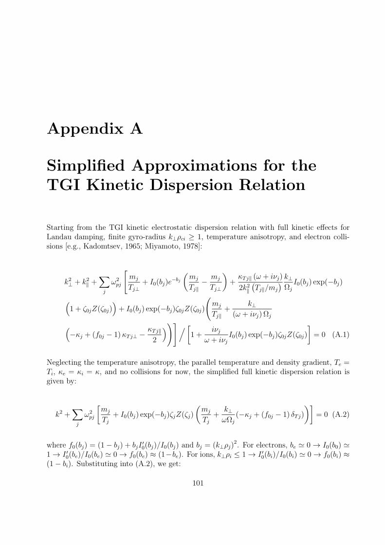
Appendix A
Simplified Approximations for theTGI Kinetic Dispersion Relation
Starting from the TGI kinetic electrostatic dispersion relation with full kinetic effects forLandau damping, finite gyro-radius k⊥ρci ≥ 1, temperature anisotropy, and electron colli-sions [e.g., Kadomtsev, 1965; Miyamoto, 1978]:
k2⊥ + k2∥ +∑j
ω2pj
[mj
Tj⊥+ I0(bj)e
−bj
(mj
Tj∥− mj
Tj⊥
)+κTj∥ (ω + iνj)
2k2∥(Tj∥/mj
) k⊥Ωj
I0(bj) exp(−bj)
(1 + ζ0jZ(ζ0j)
)+ I0(bj) exp(−bj)ζ0jZ(ζ0j)
(mj
Tj∥+
k⊥(ω + iνj) Ωj(
−κj + (f0j − 1)κTj⊥ −κTj∥
2
))]/[1 +
iνjω + iνj
I0(bj) exp(−bj)ζ0jZ(ζ0j)]= 0 (A.1)
Neglecting the temperature anisotropy, the parallel temperature and density gradient, Te =Ti, κe = κi = κ, and no collisions for now, the simplified full kinetic dispersion relation isgiven by:
k2 +∑j
ω2pj
[mj
Tj+ I0(bj) exp(−bj)ζjZ(ζj)
(mj
Tj+
k⊥ωΩj
(−κj + (f0j − 1) δTj)
)]= 0 (A.2)
where f0(bj) = (1− bj) + bjI′0(bj)/I0(bj) and bj = (k⊥ρj)
2. For electrons, be ≃ 0 → I0(b0) ≃1 → I ′0(be)/I0(be) ≃ 0 → f0(be) ≈ (1−be). For ions, k⊥ρi ≤ 1 → I ′0(bi)/I0(bi) ≃ 0 → f0(bi) ≈(1− bi). Substituting into (A.2), we get:
101
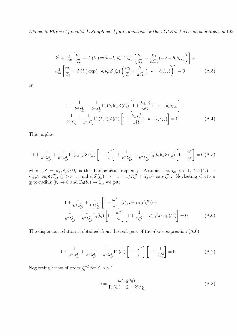
Ahmed S. Eltrass Appendix A. Simplified Approximations for the TGI Kinetic Dispersion Relation 102
k2 + ω2pe
[me
Te+ I0(be) exp(−be)ζeZ(ζe)
(me
Te+
k⊥ωΩe
(−κ− beδTe)
)]+
ω2pi
[mi
Ti+ I0(bi) exp(−bi)ζiZ(ζi)
(mi
Ti+
k⊥ωΩi
(−κ− biδTi)
)]= 0 (A.3)
or
1 +1
k2λ2D+
1
k2λ2DΓ0(be)ζeZ(ζe)
[1 +
k⊥υ2te
ωΩe
(−κ− beδTe)
]+
1
k2λ2D+
1
k2λ2DΓ0(bi)ζiZ(ζi)
[1 +
k⊥υ2ti
ωΩi
(−κ− biδTi)
]= 0 (A.4)
This implies
1 +1
k2λ2D+
1
k2λ2DΓ0(be)ζeZ(ζe)
[1− ω∗
ω
]+
1
k2λ2D+
1
k2λ2DΓ0(bi)ζiZ(ζi)
[1− ω∗
ω
]= 0 (A.5)
where ω∗ = k⊥υ2teκ/Ωe is the diamagnetic frequency. Assume that ζe << 1, ζeZ(ζe) →
iζe√π exp(ζ2e ), ζi >> 1, and ζiZ(ζi) → −1 − 1/2ζ2i + iζi
√π exp(ζ2i ). Neglecting electron
gyro-radius (be → 0 and Γ0(be) → 1), we get:
1 +1
k2λ2D+
1
k2λ2D
[1− ω∗
ω
](iζe
√π exp(ζ2e )) +
1
k2λ2D− 1
k2λ2DΓ0(bi)
[1− ω∗
ω
] [1 +
1
2ζ2i− iζi
√π exp(ζ2i )
]= 0 (A.6)
The dispersion relation is obtained from the real part of the above expression (A.6)
1 +1
k2λ2D+
1
k2λ2D− 1
k2λ2DΓ0(bi)
[1− ω∗
ω
] [1 +
1
2ζ2i
]= 0 (A.7)
Neglecting terms of order ζ−2i for ζi >> 1
ω =ω∗Γ0(bi)
Γ0(bi)− 2− k2λ2D(A.8)
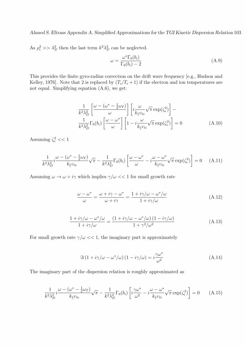
Ahmed S. Eltrass Appendix A. Simplified Approximations for the TGI Kinetic Dispersion Relation 103
As ρ2i >> λ2D then the last term k2λ2D can be neglected.
ω =ω∗Γ0(bi)
Γ0(bi)− 2(A.9)
This provides the finite gyro-radius correction on the drift wave frequency [e.g., Hudson andKelley, 1976]. Note that 2 is replaced by (Ti/Te+1) if the electron and ion temperatures arenot equal. Simplifying equation (A.6), we get:
1
k2λ2D
[ω − (ω∗ − 1
2ωT )
ω
] [iω
k∥υte
√π exp(ζ2e )
]−
1
k2λ2DΓ0(bi)
[ω − ω∗
ω
] [1− i
ω
k∥υti
√π exp(ζ2i )
]= 0 (A.10)
Assuming ζ2e << 1
1
k2λ2Diω − (ω∗ − 1
2ωT )
k∥υte
√π − 1
k2λ2DΓ0(bi)
[ω − ω∗
ω− i
ω − ω∗
k∥υti
√π exp(ζ2i )
]= 0 (A.11)
Assuming ω → ω + iγ which implies γ/ω << 1 for small growth rate
ω − ω∗
ω=ω + iγ − ω∗
ω + iγ=
1 + iγ/ω − ω∗/ω
1 + iγ/ω(A.12)
1 + iγ/ω − ω∗/ω
1 + iγ/ω=
(1 + iγ/ω − ω∗/ω) (1− iγ/ω)
1 + γ2/ω2(A.13)
For small growth rate γ/ω << 1, the imaginary part is approximately
ℑ (1 + iγ/ω − ω∗/ω) (1− iγ/ω) = iγω∗
ω2(A.14)
The imaginary part of the dispersion relation is roughly approximated as
1
k2λ2Diω − (ω∗ − 1
2ωT )
k∥υte
√π − 1
k2λ2DΓ0(bi)
[iγω∗
ω2− i
ω − ω∗
k∥υti
√π exp(ζ2i )
]= 0 (A.15)

Ahmed S. Eltrass Appendix A. Simplified Approximations for the TGI Kinetic Dispersion Relation 104
The solution for the collisionless growth rate is therefore
γ =
√πω2
Γ0(bi)ω∗
[ω − (ω∗ − 1
2ωT )
k∥υte− ω − ω∗
k∥υtiΓ0(bi) exp(ζ
2i )
](A.16)
The quadratic behavior in the growth rate can be seen in equation (A.16). Note that thesecond term in equation (A.16) is the universal growth of the drift wave. Equation (A.16)also includes the ion Landau damping effect, which is small outside the damping regimeζi >> 1. Considering the first term in the growth rate expression (A.16), we get:
γ =
√πω2
Γ0(bi)ω∗
[ω − (ω∗ − 1
2ωT )
k∥υte
](A.17)
Since there is a little modification from the diamagnetic drift velocity caused by the densitygradient, assume that ω− (ω∗ − 1
2ωT ) ≈ −1
2ωT/ω
∗ and substitute in (A.17). Then, the wavefrequency ω can be expressed as:
ω =ω∗Γ0(bi)
Γ0(bi)− 2→ ω − ω∗ =
2ω∗
Γ0(bi)− 2(A.18)
Then the collisionless growth rate is given by:
γ =
√πω∗ωTΓ0(bi)
[Γ0(bi)− 2]3 k∥υte(A.19)
In order to incorporate the collisional effects in the ionosphere, the total electron collisionfrequency νe is included in the dispersion relation (A.5) as follows:
1 +
1k2λ2
D+ 1
k2λ2DΓ0(be)ζeZ(ζe)
[1− ω∗+ 1
2ωT
ω+iνe
]1 + iνe
ω+iνeΓ0(be)ζeZ(ζe)
+
1
k2λ2D+
1
k2λ2DΓ0(bi)ζiZ(ζi)
[1− ω∗
ω
]= 0 (A.20)
where ζe = (ω + iνe)/k∥υte. Assume as before be → 0, Γ0(be) → 1 and ω ≈ ω∗ << νe, thus,ζe = iνe/k∥υte. However, ζe >> 1 and ζeZ(ζe) → −1 − 1/2ζ2e + iζe
√π exp(ζ2e ) which is still
true for the ion functions as before. Now the dispersion relation (A.20) could be written as:
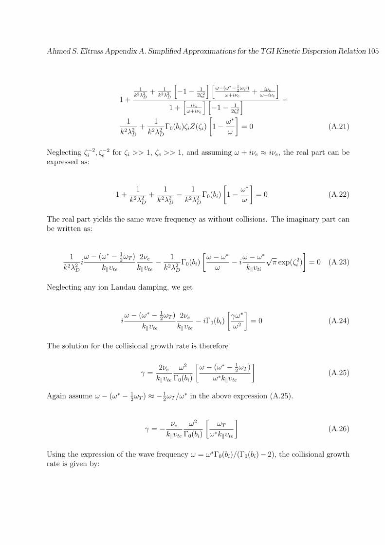
Ahmed S. Eltrass Appendix A. Simplified Approximations for the TGI Kinetic Dispersion Relation 105
1 +
1k2λ2
D+ 1
k2λ2D
[−1− 1
2ζ2e
] [ω−(ω∗− 1
2ωT )
ω+iνe+ iνe
ω+iνe
]1 +
[iνe
ω+iνe
] [−1− 1
2ζ2e
] +
1
k2λ2D+
1
k2λ2DΓ0(bi)ζiZ(ζi)
[1− ω∗
ω
]= 0 (A.21)
Neglecting ζ−2i , ζ−2
e for ζi >> 1, ζe >> 1, and assuming ω + iνe ≈ iνe, the real part can beexpressed as:
1 +1
k2λ2D+
1
k2λ2D− 1
k2λ2DΓ0(bi)
[1− ω∗
ω
]= 0 (A.22)
The real part yields the same wave frequency as without collisions. The imaginary part canbe written as:
1
k2λ2Diω − (ω∗ − 1
2ωT )
k∥υte
2νek∥υte
− 1
k2λ2DΓ0(bi)
[ω − ω∗
ω− i
ω − ω∗
k∥υti
√π exp(ζ2i )
]= 0 (A.23)
Neglecting any ion Landau damping, we get
iω − (ω∗ − 1
2ωT )
k∥υte
2νek∥υte
− iΓ0(bi)
[γω∗
ω2
]= 0 (A.24)
The solution for the collisional growth rate is therefore
γ =2νek∥υte
ω2
Γ0(bi)
[ω − (ω∗ − 1
2ωT )
ω∗k∥υte
](A.25)
Again assume ω − (ω∗ − 12ωT ) ≈ −1
2ωT/ω
∗ in the above expression (A.25).
γ = − νek∥υte
ω2
Γ0(bi)
[ωT
ω∗k∥υte
](A.26)
Using the expression of the wave frequency ω = ω∗Γ0(bi)/(Γ0(bi)− 2), the collisional growthrate is given by:

Ahmed S. Eltrass Appendix A. Simplified Approximations for the TGI Kinetic Dispersion Relation 106
γ =2νeω
∗ωTΓ0(bi)
[Γ0(bi)− 2]2 k2∥υ2te
(A.27)
For τ = Te/Ti = 1, the general expressions for the TGI collisional wave frequency and growthrate are given by:
ω =ω∗Γ0(bi)
Γ0(bi)− (1 + τ)(A.28)
γ =2νeω
∗ωTΓ0(bi)
[Γ0(bi)− (1 + τ)]2 k2∥υ2te
(A.29)
The growth rate expression (A.29) has a quadratic behavior for long wavelengths. Thegrowth rate maximizes for short wavelengths due to finite gyro-radius effects. These resultsare consistent with Federici et al. [1987]. The results in equations (A.28) and (A.29) reduceto that of Hudson and Kelley [1976] in the long wavelength regime k⊥ρci << 1, whichcorresponds to λ >> 15 m.
Appendix B
Numerical Analysis for InstabilityKinetic Dispersion Relations
The purpose of this appendix is to outline the numerical analysis of the electrostatic disper-sion relations for both the Temperature Gradient Instability (TGI) and the Gradient DriftInstability (GDI). The TGI and GDI dispersion relations presented in Chapter 3 are solvednumerically to obtain the growth rate and wave frequency. An improved root finding schemeis employed by combining the Bisection and Newton-Raphson techniques. First, the Bisec-tion method assumes the root is bracketed in an interval [a, b], then the Newton-Raphsonmethod attempts to find the root utilizing its rapid convergence rate. If the root estimatefalls outside the interval [a, b], then the Bisection method is used to narrow the intervalsufficiently such that the Newton-Raphson method will converge.
The plasma dispersion function Z(ζj) in both the TGI and GDI dispersion relations is approx-imated using the Pade method [e.g., Ronnmark, 1982, 1983]. The rational approximationsresulted from this method are suitable for numerical solution. Note that the derivatives ofthe susceptibilities with respect to ω are also needed to solve the dispersion relations becauseNewton’s method requires the derivative. These derivatives are obtained using the form ofRonnmark [1982]. Since the GDI dispersion relation is more complicated than the TGI one,it will be investigated in further detail. The kinetic dispersion relation of GDI includingfinite ion gyro-radius effects is given by [Gary and Cole, 1983]:
1 +∑j
k2Dj
k2
[1 +
(ω − kυnj − kυpj)Aj(k, ω)−Nj(k, ω)
1 + νjAj(k, ω)− i (υpj/υtj)Rxj(k, ω
]= 0 (B.1)
where
Aj(k, ω) =1√
2k∥υtj
∞∑n=−∞
Γn(bj)Z(ζjn) (B.2)
107
Ahmed S. Eltrass Appendix B. Numerical Analysis for Instability Kinetic Dispersion Relations 108
Rxj(k, ω) =ik⊥υtj√2k∥υtj
∞∑n=−∞
Z(ζjn) [Γn(bj)− Γ′n(bj)] (B.3)
Ryj(k, ω) =1√
2k∥υtj
Ω2j
k⊥υtj
∞∑n=−∞
nΓn(bj)Z(ζjn) (B.4)
and
N(k, ω) =ω(υnj + υpj)
Ωj
Ryj(k, ω) +ωνjυnjΩ2
jυtjRxj(k, ω) (B.5)
Here j = e, i stands for electron or ion. bi = (k⊥ρci)2, ζjn = (ω + nΩj)/
√2k∥υtj, ζj0 =
(ω)/√2k∥υtj, Γn(bj) = In(bj) exp(−bj), and Z(ζj) is the plasma dispersion function. By
introducing a Pade approximant for the plasma dispersion function Z(ζjn), the infinite sumsof Bessel functions of Aj(k, ω) and Rj(k, ω) can be reduced to a summable form. In thisappendix it is required to derive expressions of the infinite sums that can be used in numericalsolution of the GDI dispersion relation. It is required to prove that:
∞∑n=−∞
Γn(bj)Z(ζjn) =8∑
m=1
rmk∥ρjbjY 2
(R(Y, bj) +
Y
bj
)(B.6)
Here Z(x) =∑8
m=1 rm/(x−cm) and Y = ω/Ωce(mi/me)−cmk∥ρce√mi/me, where rm and cm
are the residues and poles of Pade approximant [Ronnmark, 1983], respectively. Substitutingin the left-hand-side of (B.6), we get:
∞∑n=−∞
Γn(bi)Z
(ω/Ωce − n(me/mi)
k∥ρce√me/mi
)
=∞∑
n=−∞
Γn(bi)8∑
m=1
rm
(ω/Ωce − n(me/mi)) /(k∥ρce
√me/mi
)− cm
=∞∑
n=−∞
Γn(bi)8∑
m=1
rmk∥ρce√me/mi
ω/Ωce − n(me/mi)− cmk∥ρce√me/mi
Ahmed S. Eltrass Appendix B. Numerical Analysis for Instability Kinetic Dispersion Relations 109
=8∑
m=1
rmk∥ρce√me/mi
∞∑n=−∞
Γn(bi)
ω/Ωce − n(me/mi)− cmk∥ρce√me/mi
=8∑
m=1
rmk∥ρce√me/mi
∞∑n=−∞
Γn(bi)
ω/Ωce(mi/me)− n− cmk∥ρce√mi/me
=8∑
m=1
rmk∥ρce√mi/me
∞∑n=−∞
Γn(bi)(mi/me)
ω/Ωce(mi/me)− n− cmk∥ρce√mi/me
(B.7)
Let Y = ω/Ωce(mi/me)− cmk∥ρce√mi/me, we get:
∞∑n=−∞
Γn(bi)Z
(ω/Ωce − n(me/mi)
k∥ρce√me/mi
)=
8∑m=1
rmk∥ρce√mi/me
∞∑n=−∞
Γn(bi)
Y − n(B.8)
Since∑∞
n=−∞ Γn = 1, we get:
∞∑n=−∞
nΓn
Y − n+ 1 =
∞∑n=−∞
(nΓn
Y − n+ Γn
)(B.9)
so,
∞∑n=−∞
nΓn
Y − n+ 1 =
∞∑n=−∞
(nΓn
Y − n+ Γn
Y − n
Y − n
)(B.10)
therefore,
∞∑n=−∞
nΓn
Y − n= Y
∞∑n=−∞
nΓn
Y − n− 1 (B.11)
also,
∞∑n=−∞
n2Γn
Y − n= −
∞∑n=−∞
((Y 2 − n2)Γn
Y − n− Y 2 Γn
Y − n
)
Ahmed S. Eltrass Appendix B. Numerical Analysis for Instability Kinetic Dispersion Relations 110
= −∞∑
n=−∞
[(Y + n)Γn − Y 2 Γn
Y − n
]= −Y + Y 2
∞∑n=−∞
Γn
Y − n(B.12)
Since∑∞
n=−∞ nΓn = 0 and Γn = Γ−n, we obtain:
Y∞∑
n=−∞
Γn
Y − n=
1
Y
∞∑n=−∞
n2Γn
Y − n+ 1 (B.13)
thus,
∞∑n=−∞
Γn(bi)
Y − n=
1
Y 2
∞∑n=−∞
n2Γn(bi)
Y − n+
1
Y(B.14)
Substituting in the right-hand-side of (B.8), we get:
∞∑n=−∞
Γn(bi)Z
(ω/Ωce − n(me/mi)
k∥ρce√me/mi
)=
8∑m=1
rmk∥ρce√mi/me
(1
Y 2
∞∑n=−∞
n2Γn(bi)
Y − n+
1
Y
)
=8∑
m=1
rmk∥ρce√mi/me
(biY 2
∞∑n=−∞
n2Γn(bi)
bi(Y − n)+
1
Y
)
=8∑
m=1
rmk∥ρce√mi/mebi
Y 2
(∞∑
n=−∞
n2Γn(bi)
bi(Y − n)+Y
bi
)(B.15)
The form of the function R(Y, bi) of Ronnmark [1983] is given by:
R(Y, bi) =∞∑
n=−∞
n2Γn(bi)
bi(Y − n)(B.16)
Substituting in the right-hand-side of (B.15), we prove that
∞∑n=−∞
Γn(bi)Z
(ω/Ωce − n(me/mi)
k∥ρce√mi/me
)=
8∑m=1
rmk∥ρce√mi/mebi
Y 2
(R(Y, bi) +
Y
bi
)(B.17)
Ahmed S. Eltrass Appendix B. Numerical Analysis for Instability Kinetic Dispersion Relations 111
Substituting from (B.17) into (B.2, B.3, and B.4), we finally get the expressions that will beused in numerical solution of the GDI dispersion relation:
Aj(k, ω) =1√
2k∥υtj
8∑m=1
rmk∥ρjbjY 2
(R(Y, bj) +
Y
bj
)(B.18)
Rxj(k, ω) =ik⊥υtj√2k∥υtj
[1√
2k∥υtj
8∑m=1
rmk∥ρjbjY 2
(R(Y, bj) +
Y
bj
)−
8∑m=1
rmk∥ρj
∞∑n=−∞
Γ′n(bj)
Y − n
]
=ik⊥υtj√2k∥υtj
[1√
2k∥υtj
8∑m=1
rmk∥ρjbjY 2
(R(Y, bj) +
Y
bj
)−
8∑m=1
rmk∥ρjY 2
R′(Y, bj)
](B.19)
Ryj(k, ω) =1√
2k∥υtj
Ω2j
k⊥υtj
8∑m=1
rmk∥ρjbjY
R(Y, bj) (B.20)
The resulting expressions are valid for all real k and well suited for numerical solution. Asmentioned previously, the derivatives of the susceptibilities with respect to ω are needed tosolve the GDI dispersion relation. They are obtained using the form of Ronnmark [1982].
Appendix C
A Description of the ElectrostaticGyro-Kinetic Simulation Model
C.1 Plasma Simulation Algorithm
In this section, we briefly discuss the two-dimensional Particle-In-Cell (PIC) electrostaticplasma simulation model used in this study. As shown in Figure C.1, the simulation boxis defined in physical space, thus two spatial dimensions x and y are assumed. The plasmalength in both x- and y-directions Lx and Ly are divided into the number of grid cellsnx and ny, respectively. Thus, there are nx + 1 and ny + 1 grid points in the x- and y-directions, respectively. The index i is used to denote grid points in the x-direction and theindex j for the y-direction. The parameters ∆x and ∆y are Lx/nx and Ly/ny, respectively.The Particle-In-Cell (PIC) electrostatic computational cycle with collisional effects used inthis study is shown in Figure C.2. The algorithm used in the computational loop involvesthe basic steps of advancing position and velocity of species, calculating charge density,calculating potential and electric fields, and interpolating fields to grid points.
The nonlinear gyro-averaged Vlasov-Poisson system of equations are solved using Particle-In-Cell (PIC) simulation methods. This can be summarized as follows:
• Initialize particles in coordinate and velocity space (uniform electron and ion density withno background E field) and calculate the fields at t = 0.
• Advance the particle velocities in the presence of the electric field from the Lorentz forceequation. The parallel acceleration for electrons and ions can be expressed as:
electron : υn+1/2∥ = υ
n−1/2∥ +
q
mEn
∥ dt (C.1)
112
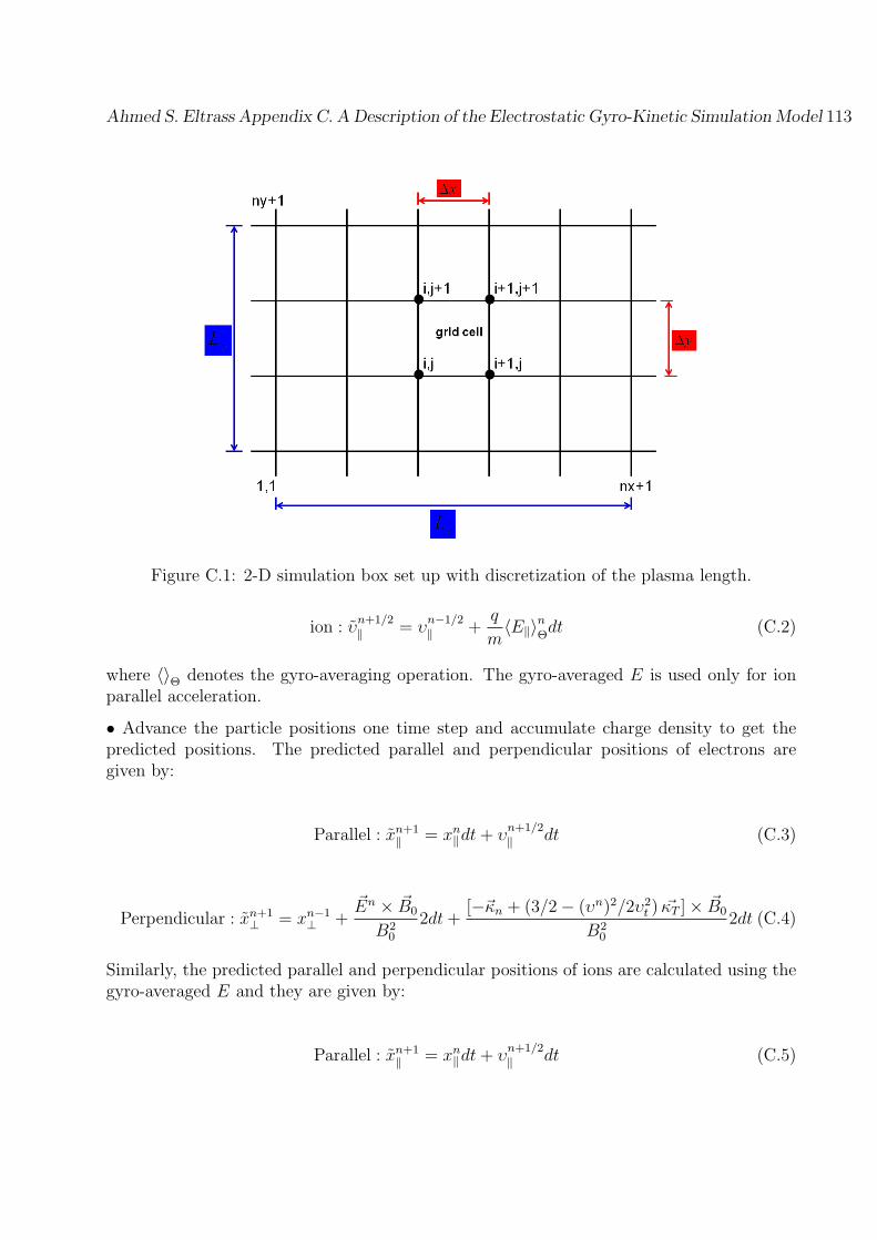
Ahmed S. Eltrass Appendix C. A Description of the Electrostatic Gyro-Kinetic Simulation Model 113
Figure C.1: 2-D simulation box set up with discretization of the plasma length.
ion : υn+1/2∥ = υ
n−1/2∥ +
q
m⟨E∥⟩nΘdt (C.2)
where ⟨⟩Θ denotes the gyro-averaging operation. The gyro-averaged E is used only for ionparallel acceleration.
• Advance the particle positions one time step and accumulate charge density to get thepredicted positions. The predicted parallel and perpendicular positions of electrons aregiven by:
Parallel : xn+1∥ = xn∥dt+ υ
n+1/2∥ dt (C.3)
Perpendicular : xn+1⊥ = xn−1
⊥ +En × B0
B20
2dt+[−κn + (3/2− (υn)2/2υ2t ) κT ]× B0
B20
2dt (C.4)
Similarly, the predicted parallel and perpendicular positions of ions are calculated using thegyro-averaged E and they are given by:
Parallel : xn+1∥ = xn∥dt+ υ
n+1/2∥ dt (C.5)

Ahmed S. Eltrass Appendix C. A Description of the Electrostatic Gyro-Kinetic Simulation Model 114
Figure C.2: Computational cycle for the Particle-In-Cell (PIC) gyro-kinetic simulation modelwith collisional effects.
Perpendicular : xn+1⊥ = xn−1
⊥ +⟨E⟩
n
Θ × B0
B20
2dt+[−κn + (3/2− (υn)2/2υ2t ) κT ]× B0
B20
2dt(C.6)
where, En is the weighted electric field at time n, (υn)2 = (υn⊥)2 + (υn∥ )
2 is the total velocity.The total velocity can be approximated from averaging the parallel velocity and the right-hand-side of equation (C.6). The predicted electron densities ne and ion gyro-averageddensities ¯ni are calculated using the predicted positions.
• Calculate the predicted potential and electric field from the Vlasov and modified Poisson’sequations. The electrostatic gyro-kinetic potential equation in the particle variable spacecan be expressed as [e.g., Lee, 1987]:
∇2Φ− τ
(Φ− Φ
)λ2D
+
(ρsλD
)2
∇⊥ ·[(ni − n0)
n0
∇⊥Φ
]=
−e(ni − ne)
ϵ0(C.7)
The gyro-averaged Poisson equation is solved in the spectral domain (kx, ky) using pseu-dospectral methods [Appendix C.2] to obtain the predicted potential at guiding center:
Ahmed S. Eltrass Appendix C. A Description of the Electrostatic Gyro-Kinetic Simulation Model 115
(kλD)2δΦk + τ
[1− Γ0(k
2ρ2ci)]δΦk +
ρ2ci
[(ikδnik)⊗ (ikδΦk) + δnik ⊗ k2δΦk
]= δnik − δnek (C.8)
or
δΦk =
[δnik − δnek
]− ρ2ci
[(ikδnik)⊗ (ikδΦk) + δnik ⊗ k2δΦk
](kλD)2 + τ [1− Γ0(k2ρ2ci)]
(C.9)
This equation is solved iteratively with the use of pseudospectral methods [Appendix C.2] toperform the convolution ⊗ operation. Then, the predicted gyro-averaged potential at timen+ 1 is:
ψ(R) = Φ(R)− q
2T
(υtΩ
)2|∂Φ(R)∂R⊥
|2 (C.10)
The predicted electric field E = −∇ψ is calculated in the spatial domain as follows:
For electrons : En+1/2 =(En+1 + En
)/2 (C.11)
For ions : ⟨E⟩n+1/2Θ =
(⟨E⟩n+1
Θ + ⟨E⟩nΘ)/2 (C.12)
After the predicted electric field is calculated, it is interpolated back to the particle position.
• Calculate the corrected electron and ion positions and the gyro-averaged ion density uti-lizing the predicted gyro-averaged field at the half time step. The ion and electron correctedpositions xn+1
⊥ are calculated by correctly time centering as follows:
electron : xn+1⊥ = xn⊥ +
En+1/2 × B0
B20
dt+
[−κn +
(3/2− (υn+1/2)2/2υ2t
)κT]× B0
B20
dt(C.13)
ion : xn+1⊥ = xn⊥ +
⟨E⟩n+1/2
Θ × B0
B20
dt+
[−κn +
(3/2− (υn+1/2)2/2υ2t
)κT]× B0
B20
dt (C.14)
Ahmed S. Eltrass Appendix C. A Description of the Electrostatic Gyro-Kinetic Simulation Model 116
where, x = x⊥ + x∥b is the total position.
• Use the gyro-averaged modified Poisson equation to calculate the corrected guiding centerpotential and electric field using the corrected gyro-averaged ion density and electron density.
δΦk =
[δnik − δnek
]− ρ2ci
[(ikδnik)⊗ (ikδΦk) + δnik ⊗ k2δΦk
](kλD)2 + τ [1− Γ0(k2ρ2ci)]
(C.15)
Then, the corrected gyro-averaged potential at time n+ 1 is calculated as follows:
ψ(R) = Φ(R)− q
2T
(υtΩ
)2|∂Φ(R)∂R⊥
|2 (C.16)
Finally, the corrected electric field E = −∇ψ is calculated in the spatial domain.
C.2 Spectral and Pseudospectral Methods
Discretization techniques of differential equations comprise three methods: finite differenceapproximation, finite element approximation, and spectral methods. Spectral methods aremuch faster than other discretization techniques in that they need less grid points to producea comparably accurate solution [Orszag, 1971a]. Spectral methods are the best choice forsimulations involving nonlinear terms such as turbulence studies and ionospheric plasmainstabilities.
The forward and inverse Fourier Transform equations in a continuous domain, respectively,are given by:
H(k) =
∫ ∞
−∞h(x)e2πikxdx (C.17)
h(x) =
∫ ∞
−∞H(k)e−2πikxdx (C.18)
Assume that h(x) is a continuous function with a bandwidth less than the Nyquist criticalwave number kc = 1/2∆x. The function h(x) is sampled at evenly spaced and discrete timeintervals ∆x and is expressed as:
h(x) = ∆x∞∑
n=−∞
hnsin [2πkc(x− n∆x)]
π(x− n∆x)(C.19)
Ahmed S. Eltrass Appendix C. A Description of the Electrostatic Gyro-Kinetic Simulation Model 117
where
hj = h(xj), xj = j∆x, j = 0, 1, 2, ....N − 1 (C.20)
The points hj are called nodes or grid points. The discrete Fourier coefficients of N pointscomplex-valued function are given by:
H(kn) =
∫ ∞
−∞h(x)e2πikxdx ≃
N−1∑j=0
hj∆xe2πiknxj = ∆x
N−1∑j=0
hje2πijn
N (C.21)
The Discrete Fourier Transform (DFT) of the N points function hj is expressed as
Hn =N−1∑j=0
hje2πijn
N (C.22)
The Inverse Discrete Fourier Transform (IDFT) is given by:
hj =1
N
N−1∑n=0
Hne−2πijn
N (C.23)
The N-point DFT has been computed using an algorithm called the Fast Fourier Transform(FFT) [Press et al., 1992], which is very fast and efficient approach.
Several operations are performed in the current simulation model using spectral methods asfollowing:
• Differentiation: taking a derivative in the Fourier transform space consists of simply mul-tiplying each Fourier coefficients with the imaginary unit times the corresponding wavenumber. The differentiation of a function in Fourier space is given by:
Fdhdx
= ikhk (C.24)
where, F denotes the Fourier Transform operation and k is the Fourier wave number.
• Laplacian (∇2): since ∇2 = ∂2
∂x2 +∂2
∂y2in 2-D, the Laplacian operator in the Fourier space
becomes a multiplication of each Fourier coefficients with −k2, where k2 = k2x + k2y in 2-D.The first order derivative k and the Laplacian coefficient k2 in a continuous domain arereplaced by κ and K2 in two-dimensions [Birdsall and Langdon, 1991], respectively, where
κ = k1
[sin(k1∆x1)
k1∆x1
]k1 + k2
[sin(k2∆x2)
k2∆x2
]k2 (C.25)
Ahmed S. Eltrass Appendix C. A Description of the Electrostatic Gyro-Kinetic Simulation Model 118
and
K2 = k21
[sin(k1∆x1
2)
k1∆x1
2
]2+ k22
[sin(k2∆x2
2)
k2∆x2
2
]2(C.26)
• Convolution: nonlinear terms such as the ones found in the modified poisson equation(C.7) need a careful treatment by spectral methods. The Fourier space convolution arisesfrom products of functions u(x) and v(x) in real x space. This can be expressed as
wk =∑
p+q=k
upvq |p|, |q| ≤ N/2 (C.27)
where p, q, k are the Fourier mode numbers.
The pseudospectral method proposed by Orszag [1971a, b] utilizes suitable discrete Fouriertransforms to express wk as local product of Fourier-transformed fields. The inverse DFTgiven in (C.23) is used to transform up and vp to Ui and Vj in physical space, where Ui andVj are defined at exactly N points of xj = 2π/N for j = 0, 1, ...N − 1. Thus, Wj can beexpressed as the local product UjVj of the transform fields, and then the DFT is used toreturn to the Fourier space. This approach can be summarized as following:
uk, vkIFFT−−−→ Uj, Vj
×−→ WjFFT−−−→ wk (C.28)
The aliased convolution sum wk can be expressed as:
wk =1
N
N−1∑j=0
UjVje−ikxj =
1
N
N−1∑j=0
∑|p|≤N/2
upe−ipxj
∑|q|≤N/2
vqe−iqxj (C.29)
or
wk =∑
|p|, |q|≤N/2
upvq1
N
N−1∑j=0
e−i(p+q−k)xj (C.30)
Using the discrete transform orthogonality relation, equation (C.30) can be written as:
wk =∑
p+q=k
upvq +∑
p+q=k±N
upvq = wk +∑
p+q=k±N
upvq (C.31)
For any k < N/2, a nonzero aliasing error may occur from the discontinuity and the steepgradient effects. Patterson and Orszag [1971] showed that if the set of allowable modes used
Ahmed S. Eltrass Appendix C. A Description of the Electrostatic Gyro-Kinetic Simulation Model 119
in the convolution sum is reduced, there will not be any modes that contribute to the aliasedterms. They presented an algorithm to truncate Fourier modes that lie outside a sphere ofradius αK, where K = N/2 and α ≥ 2
√2
3≈ 0.94. Applying this approach in the current
simulation, the modes within a sphere of radius 0.94K are investigated. Truncation of themodes outside the sphere is performed using a filter of the form e−αn
[Birdsall and Langdon,1991], where α = k/kmax. This filter smoothes the boundary by attenuating the higher orderFourier coefficients. Pseudospectral approximations are much faster than spectral methodsin handling the nonlinearities. This comes from the fact that the evolution of convolutionusing spectral method requires at least twice the number of FFTs as the correspondingpseudospectral method [Orszag, 1972].
Bibliography
[1] Aarons, J., J. P. Mullen, J. P. Koster, R. F. DaSilva, J. R. Medeiros, R. T. Medeiros,A. Bushby, J. Pantoja, J. Lanat, and M. R. Paulson (1980), Seasonal and geomagneticcontrol of equatorial scintillations in two longitudinal sectors, J. Atmos. Terr. Phys., 42,861-866.
[2] Aarons, J. (1982), Global morphology of ionospheric scintillations, Proc. IEEE, 70, 360-378.
[3] Anderson, P., R. Heelis, and W. Hanson (1991), The ionospheric signatures of rapidsubauroral ion drifts, J. Geophys. Res., 96, 5785-5792.
[4] Anderson, P., W. Hanson, R. Hellis, J. D. Craven, D. Baker, and L. Frank (1993),A proposed production model of rapid subauroral ion drifts and their relationship tosubstorm evolution, J. Geophys. Res., 98, 6069-6078.
[5] Aquino, M., M. Andreotti, A. Dodson, and H. J. Strangeways (2007), On the use ofionospheric scintillation indices in conjunction with receiver tracking models, Adv. SpaceRes., doi:10.1016/j.asr.2007.05.035.
[6] Baker, K. B., R. A. Greenwald, A. D. M. Walker, P. F. Bythrow, L. J. Zanetti, T. A.Potemra, D. A. Hardy, F. J. Rich, and C. L. Rino (1986), A case study of plasma processesin the dayside cleft, J. Geophys. Res., 91(A3), 3130-3144, doi:10.1029/JA091iA03p03130.
[7] Baker, K., and S. Wing (1989), A new magnetic coordinate system for conjugate studiesat high latitudes, J. Geophys. Res., 94 (A7), 9139-9143, doi:10.1029/JA094iA07p09139.
[8] Baker, K. B., J. R. Dudeney, R. A. Greenwald, M. Pinnock, P. T. Newell, A. S. Rodger,N. Mattin, and C. I. Meng (1995), HF radar signatures of the cusp and low-latitudeboundary layer, J. Geophys. Res., 100 (A5), 7671-7695, doi:10.1029/94JA01481.
[9] Baker, D. N. (2000), Effects of the Sun on the Earth’s environment, J. Atmos. Sol. Terr.Phys., 62, 1669-1691.
[10] Baker, J. B. H., R. A. Greenwald, J. M. Ruohoniemi, K. Oksavik, J. W. Gjerloev,L. J. Paxton, and M. R. Hairston (2007), Observations of ionospheric convection from
120
Ahmed S. Eltrass Bibliography 121
the Wallops SuperDARN radar at middle-latitudes, J. Geophys. Res., 112, A01303,doi:10.1029/2006JA011982.
[11] Ballatore, P., J. P. Villain, N. Vilmer, and M. Pick (2001), The influence of the in-terplanetary medium on SuperDARN radar scattering occurrence, Ann. Geophys., 18,1576-1583.
[12] Banerjee, P. K., R. S. Dabas, and B. M. Reddy (1992), C- and L-band transionosphericscintillation experiment: some results for applications to satellite radio systems, RadioSci., 27(6), 955-969.
[13] Banola, S., B. M. Pathan, D. R. K. Rao, and H. Chandra (2005), Spectral characteristicsof scintillations producing ionospheric irregularities in the Indian region, Earth PlanetsSpace, 57, 47-59.
[14] Barthes, L., R. Andre, J. C. Cerisier, and J. P. Villain (1998), Separation of multipleechoes using a high-resolution spectral analysis for SuperDARN HF radars, Radio Sci.,33 (4), 1005-1017, doi:10.1029/98RS00714.
[15] Basu, S., J. Aarons, J. P. McClure, and M. D. Cousins (1978), On the coexistence ofkilometers and meter-scale irregularities in the nighttime equatorial F-region, J. Geophys.Res., 83, 4219-4226.
[16] Basu, S., J. P. McClure, and W. B. Hanson (1983), High resolution top-side data ofelectron densities and/GHz scintillations in the equatorial region, J. Geophys. Res., 88,403.
[17] Basu, S., E. MacKenzie, and Su. Basu (1988), Ionospheric constraints on VHF/UHFcommunication links during solar maximum and minimum periods, Radio Sci., 23, 363-378.
[18] Basu, S., C. E. Valladares, H. C. Yeh, S. Y. Su, E. MacKenzie, P. J. Sultan, J. Aarons,F. J. Rich, P. Doherty, K. M. Groves, and T. W. Bullett (2001), Ionospheric effects ofmajor magnetic storms during the International Space Weather Period of September andOctober 1999: GPS observations, VHF/UHF scintillations, and in situ density structuresat middle and equatorial latitudes, J. Geophys. Res., 106, 30, 389.
[19] Basu, S., K. M. Groves, S. Basu, and P. J. Sultan (2002), Specification and forecastingof scintillations in communication/navigation links: current status and future plans, J.Atmos. Terr. Phys., 64, 1745-1754, doi:10.1016/S1364-6826(02) 00124-4.
[20] Basu, S., J. J. Makela, E. MacKenzie, P. Doherty, J. W. Wright, F. Rich, M. J. Kesk-inen, R. E. Sheehan, and A. J. Coster (2008), Large magnetic storm-induced nighttimeionospheric flows at mid-latitudes and their impacts on GPS-based navigation systems, J.Geophys. Res., 113, A00A06, doi:10.1029/2008JA013076.
Ahmed S. Eltrass Bibliography 122
[21] Beach, T. L. (1998), Global Positioning System studies of equatorial scintillations, Ph.D.dissertation, Cornell Univ., Ithaca, N. Y.
[22] Beach, T. L. (2006), Perils of the GPS phase scintillation index (Sigma Phi), Radio Sci.,41, RS5S31, doi:10.1029/2005RS003356.
[23] Bhattacharyya, A., and R. G. Rastogi (1985), Amplitude scintillation during early andlate phases of evolution of irregularities in the nighttime equatorial ionosphere, Radio Sci.,20(4), 935-946.
[24] Bhattacharyya, A., and R. G. Rastogi (1991), Structure of ionospheric irregularitiesfrom amplitude and phase scintillation observations, Radio Sci., 26(2), 439-449.
[25] Birdsall, C. K. (1991), Particle-in-Cell charged-particle simulations Plus Monte CarloCollisions with neutral atoms, PIC-MCC, IEEE Trans. plasma sci., 19, 65-85.
[26] Birdsall, C. K., and A. B. Langdon (1991), Plasma Physics via Computer Simulation,New York: McGraw-Hill.
[27] Booker, H. G., J. A. Ratcliffe, and D. H. Shinn (1950), Diffraction from an irregularscreen with applications to ionospheric problems, Phil. Trans. R. Soc. London, Ser. A,856, 579-609.
[28] Braginskii, S. I. (1965), Transport processes in a plasma, Reviews of plasma physics, 1,205, Bureau, New York.
[29] Briggs, B. H., and I. A. Parkin (1963), On the variation of radio star and satellitescintillation with zenith angle, J. Atmos. Terr. Phys., 25, 339-365.
[30] Bristow, W. A., R. A. Greenwald, and J. P. Villain (1996), On the seasonal dependenceof medium-scale atmospheric gravity waves in the upper atmosphere at high-latitudes, J.Geophys. Res., 101(A7), 15, 685-15, 699.
[31] Buckley, R. (1975), Diffraction by a random phase-changing screen: A numerical exper-iment, J. Atmos. Terr. Phys., 37, 1431-1446.
[32] Chapman, S. (1931), The absorption and dissociative or ionizing effect of monochromaticradiation in an atmosphere on a rotating earth, Proc. Roy. SOC., London, 43, 2645;also, The absorption and dissociative or ionizing effect of monochromatic radiation in anatmosphere on a rotating earth Part II: Grazing incidence, Proc. Roy. Soc., London, 43,484-501, 1931.
[33] Chaturvedi, P. K., and S. L. Ossakow (1979), Nonlinear stabilization of the E × Bgradient drift instability in ionospheric plasma clouds, J. Geophys. Res., 84, 419.
[34] Chen, F. F. (1984), Introduction to plasma physics and controlled fusion, vol. 1, PlasmaPhysics, 2nd ed., pp. 218-223, Elsevier, New York.
Ahmed S. Eltrass Bibliography 123
[35] Chisham, G., M. Lester, S. E. Milan, M. P. Freeman, W. A. Bristow, A. Grocott,K. A. McWilliams, J. M. Ruohoniemi, T. K. Yeoman, P. L. Dyson, R. A. Greenwald,T. Kikuchi, M. Pinnock, J. P. S. Rash, N. Sato, G. J. Sofko, J. P. Villain, and A. D.M. Walker (2007), A decade of the Super Dual Auroral Radar Network (SuperDARN):scientific achievements, new techniques and future directions, Surv. Geophys., 28, 33-109.
[36] Chisham, G., T. Yeoman, and G. Sofko (2008), Mapping ionospheric backscatter mea-sured by the SuperDARN HF radars-Part 1: A new empirical virtual height model, Ann.Geophys., 26, 823-841.
[37] Clausen, L. B. N., J. B. H. Baker, J. M. Ruohoniemi, R. A. Greenwald, E. G. Thomas, S.G. Shepherd, E. R. Talaat, W. A. Bristow, Y. Zheng, A. J. Coster, and S. Sazykin (2012),Large-scale observations of a subauroral polarization stream by mid-latitude SuperDARNradars: Instantaneous longitudinal velocity variations, J. Geophys. Res., 117.
[38] Coster, A., S. Skone, C. Mitchell, G. De Franceschi, L. Alfonso, and V. Romano (2005),Global studies of GPS scintillation, paper presented at National Technical Meeting (NTM2005), Inst. of Navig., San Diego, Calif.
[39] Conker, R. S., M. B. El-Arini, C. J. Hegarty, and T. Hsiao (2003), Modelling the effectsof ionospheric scintillation on GPS/Satellite-Based Augmentation System availability, Ra-dio Sci., 38(1), 1001, doi:10.1029/2000RS002604.
[40] Cornwall, J. M., F. V. Coroniti, and R. M. Thorne (1971), Unified theory of SAR arcformation at the plasmapause, J. Geophys. Res., 76, 4428.
[41] Crane, R. K. (1977), Ionospheric scintillation, Proceedings of the IEEE, 65(2), 180-199.
[42] Crowley, G., G. Bust, A. Reynolds, I. Azeem, R. Wilder, B. W. O’Hanlon, M. L. Psiaki,S. Powell, T. E. Humphreyes, and J. A. Bhatti (2011), Cases: A novel low-cost ground-based dual-frequency gps software receiver and space weather monitor, in Proceedingsof the 24th International Technical Meeting of the Satellite Division of the Institute ofNavigation (ION GNSS 2011), pp. 1437-1446, Portland, OR, September 2011.
[43] DasGupta, A., A. Maitra, and S. K. Das (1985), Post-midnight equatorial scintillationactivity in relation to geomagnetic disturbances, J. Atmos. Terr. Phys., 47, 911-916.
[44] Davies, K. (1990), Ionospheric Radio, The Institution of Engineering and Technology,London, U. K.
[45] de Larquier, S., A. Eltrass, A. Mahmoudian, J. M. Ruohoniemi, J. B. H. Baker, W.A. Scales, P. J. Erickson, and R. A. Greenwald (2014), Investigation of the temperaturegradient instability as the source of mid-latitude quiet-time decameter-scale ionosphericirregularities: Part 1, Observations, J. Geophys. Res., 119, doi:10.1002/2013JA019643.

Ahmed S. Eltrass Bibliography 124
[46] Deshpande, K. B., G. S. Bust, C. R. Clauer, H. Kim, J. E. Macon, T. E. Humphreys,J. A. Bhatti, S. B. Musko, G. Crowley, and A. T. Weatherwax (2012), Initial GPS Scin-tillation results from CASES receiver at South Pole, Antarctica, Radio Sci., 47, RS5009,doi:10.1029/2012RS005061.
[47] Dimits, A. M., and W. W. Lee (1991), Nonlinear mechanisms for drift wave saturationand induced particle transport, Phys. Fluids., 3, 1557, doi:10.1063/1.859674.
[48] Dougherty, J. P., and D. T. Farley (1960), A theory of incoherent scattering of radiowaves by a plasma, Proceedings of the Royal Society of London, Series A. Mathematicaland Physical Sciences, 259(1296), 79-99.
[49] Drayton, R. A., A. V. Koustov, M. R. Hairston, and J. P. Villain (2005), Comparisonof DMSP cross-track ion drifts and SuperDARN line-of-sight velocities, Ann. Geophys.,23, 2479-2486, doi:10.5194/angeo-23-2479-2005.
[50] Dubin, D. H. E., J. A. Krommes, C. R. Oberman, and W. W. Lee (1983), Nonlineargyro-kinetic equations, Phys. Fluids, 26, 3524-3535.
[51] Dungey, J. W. (1956), Convective diffusion in the equatorial F-region, J. Atmos. Terr.Phys., 9, 304-310.
[52] Eltrass, A., A. Mahmoudian, W. A. Scales, S. de Larquier, J. M. Ruohoniemi, J. B.H. Baker, R. A. Greenwald, and P. J. Erickson (2014a), Investigation of the temperaturegradient instability as the source of mid-latitude quiet-time decameter-scale ionosphericirregularities: Part 2, Linear analysis, J. Geophys. Res., 119, doi:10.1002/2013JA019644.
[53] Eltrass, A., W. A. Scales, A. Mahmoudian, S. de Larquier, J. M. Ruohoniemi, J. B.H. Baker, R. A. Greenwald, and P. J. Erickson (2014b), Investigation of the generationsource of decameter-scale sub-auroral ionospheric irregularities during geomagneticallyquiet periods, In General Assembly and Scientific Symposium (URSI GASS), 2014 XXXIthURSI. IEEE., doi:10.1109/URSIGASS.2014.6929950.
[54] Eltrass, A., and W. A. Scales (2014), Nonlinear evolution of the temperaturegradient instability in the mid-latitude ionosphere, J. Geophys. Res., 119, 1-13,doi:10.1002/2014JA020314.
[55] Erickson, P. J., J. C. Foster, and J. M. Holt (2002), Inferred electric field variability inthe polarization jet from Millstone Hill E-region coherent scatter observations, Radio Sci.,37(2), 1027, doi:10.1029/2000RS002531.
[56] Evans, J. V. (1969), Theory and practice of ionosphere study by Thomson scatter radar,Proceedings of the IEEE, 57(4), 496-530.
[57] Evans, J., J. Holt, W. Oliver, and R. Wand (1983), The fossil theory of nighttime highlatitude F-region troughs, J. Geophys. Res., 88, 7769.
Ahmed S. Eltrass Bibliography 125
[58] Fang, D. J. and C. H. Liu (1984), Statistical characterizations of equatorial scintillationin the Asia region, Radio Sci., 19, 345-358.
[59] Farley, D. T. (1959), A theory of electrostatic fields in a horizontally stratified ionospheresubject to a vertical magnetic field, J. Geophys. Res., 64 (9), 1225-1233.
[60] Farley, D. T., J. P. Dougherty, and D. W. Barron (1961), A theory of incoherent scatter-ing of radio waves by a plasma II. Scattering in a magnetic field, Proceedings of the RoyalSociety of London, Series A. Mathematical and Physical Sciences, 263(1313), 238-258.
[61] Federici, J. F., W. W. Lee, and W. M. Tang (1987), Nonlinear evolution of drift insta-bilities in the presence of collisions, Phys. Fluids., 30, 425, doi:10.1063/1.866393.
[62] Fejer, B. G., and M. C. Kelley (1980), Ionospheric irregularities, Rev. Geophys., 18(2),401-454, doi:10.1029/RG018i002p00401.
[63] Forte, B. (2005), Optimum detrending of raw GPS data for scintillation mea-surements at auroral latitudes, J. Atmos. Sol. Terr. Phys., 67(12), 1100-1109,doi:10.1016/j.jastp.2005.01.011.
[64] Forte, B., and S. M. Radicella (2002), Problems in data treatment for ionospheric scin-tillation measurements, Radio Sci., 37(6), 1096, doi:10.1029/2001RS002508.
[65] Foster, J. C., and F. J. Rich (1998), Prompt mid-latitude electric field effects duringsevere magnetic storms, J. Geophys. Res., 103, 26367-26372.
[66] Foster, J. C., and W. J. Burke (2002), SAPS: A new categorization for subauroralelectric fields, Eos, Trans. AGU, 83(36), 393-394.
[67] Foster, J. C., P. J. Erickson, A. J. Coster, J. Goldstein, and F. J. Rich (2002),Ionospheric signatures of plasmaspheric tails, Geophys. Res. Lett., 29(13), 1623,doi:10.1029/2002GL015067.
[68] Foster, J. C., and H. B. Vo (2002), Average characteristics and activity de-pendence of the subauroral polarization stream, J. Geophys. Res., 107(A12), 1475,doi:10.1029/2002JA009409.
[69] Foster, J., P. Erickson, F. Lind, and W. Rideout (2004), Millstone Hill coherent-scatterradar observations of electric field variability in the sub-auroral polarization stream, Geo-phys. Res. Lett., 31, L21803, doi:10.1029/2004GL021271.
[70] Fukao, S., M. C. Kelley, T. Shirakawa, T. Takami, M. Yamomoto, T. Tsuda, and S.Kato (1991), Turbulent upwelling of the mid-latitude ionosphere: 1. Observational resultsby the MU radar, J. Geophys. Res., 96, 2735-3746.
[71] Gary, S. P., and M. F. Thomsen (1982), Collisionless electrostatic interchange instabil-ities, J. Plasma Phys., 28(03), 551-564.
Ahmed S. Eltrass Bibliography 126
[72] Gary, S. P., and T. E. Cole (1983), Pedersen density drift instabilities, J. Geophys. Res.,Vol. 88, No. A12, pp.10, 104-10, 110.
[73] Gillies, R. G., G. C. Hussey, G. J. Sofko, D. M. Wright, and J. A. Davies (2010),A comparison of EISCAT and SuperDARN F-region measurements with considera-tion of the refractive index in the scattering volume, J. Geophys. Res., 115, A06319,doi:10.1029/2009JA014694.
[74] Gordon, W. E. (1958), Incoherent scattering of radio waves by free electrons with ap-plications to space exploration by radar, Proceedings of the IRE, 46(11), 1824-1829.
[75] Greenwald , R. A., K. B. Baker, R. A. Hutchins, and C. Hanuise (1985), An HF phased-array radar for studying small-scale structure in the high-latitude ionosphere, Radio. Sci,20(1), 63-79.
[76] Greenwald, R. A., K. B. Baker, J. R. Dudeney, M. Pinnock, T. B. Jones, E. C.Thomas, J. P. Villain, J. C. Cerisier, C. Senior, C. Hanuise, R. D. Hunsuker, G. Sofko,J. Koehler, E. Nielsen, R. Pellinen, A. D. M. Walker, N. Sato, and H. Yamagishi (1995),DARN/SuperDARN: A global view of the dynamics of high-latitude convection, SpaceSci. Rev., 71, 763-796.
[77] Greenwald, R. A., K. Oksavik, P. J. Erickson, F. D. Lind, J. M. Ruohoniemi, J. B.H. Baker, and J. W. Gjerloev (2006), Identification of the temperature gradient instabil-ity as the source of decameter-scale ionospheric irregularities on plasmapause field lines,Geophys. Res. Lett., VOL. 33, L18105, doi:10.1029/2006GL026581.84, 419.
[78] Gurnett, D. A., G. W. Pfeiffer, R. R. Anderson, S. R. Mosier, and D. P. Cauffman(1969), Initial observations of VLF electric and magnetic fields with the Injun 5 spacecraft,J. Geophys. Res., 74, 4631.
[79] Guzdar, P. N., N. A. Gondarenko, P. K. Chaturvedi, and S. Basu (1998), Three-dimensional nonlinear simulations of the gradient drift instability in the high-latitudeionosphere, Radio Sci., 33, 1901-1913.
[80] Gwal, A. K., S. Dubey, and R. Wahi (2004), A study of L-band scintillations at equa-torial latitudes, volume 34 of Advances in Space Research, pages 2092- 2095, Pergamon-Elsevier Science Ltd, Kidlington.
[81] Hajj, G. A., B. D. Wilson, C. Wang, X. Pi, and I. G. Rosen (2004), Data assimilationof ground GPS total electron content into a physics-based ionospheric model by use of theKalman filter, Radio Sci., 39, RS1S05, doi:10.1029/2002RS002859.
[82] Hanuise, C., J. P. Villain, D. Gresillon, B. Cabrit, R. A. Greenwald, and K. B. Baker(1993), Interpretation of HF radar ionospheric Doppler spectra by collective wave scatter-ing theory, Annales Geophysicae, 11 (1), 29-39.
Ahmed S. Eltrass Bibliography 127
[83] Hargreaves, J. K. (1979), The upper atmosphere and solar terrestrial relations- Anintroduction to the aerospace environment, Van Nostrand Reinhold Co., New York, 312p. 1.
[84] Henderson, M. G., E. F. Donovan, J. C. Foster, I. R. Mann, T. J. Immel, S. B. Mende,and J. B. Sigwarth (2010), Start-to-end global imaging of a sunward propagating, SAP-Sassociated giant undulation event, J. Geophys. Res., doi:10.1029/2009JA014106.
[85] Hofmann-Wellenhof, B., H. Lichtengegger, and J. Collins (2001), GPS Theory and Prac-tice, 5th edition, Wien: Springer Verlag, New York.
[86] Hoh, F. C. (1963), Instability of a Penning discharge, Phys. Fluids, 6, 1184.
[87] Hosokawa, K., T. Iyemori, A. S. Yukimatu, and N. Sato (2001), Source of field-alignedirregularities in the subauroral F-region as observed by the SuperDARN radars, J. Geo-phys. Res., 106(A11), 24, 713-24, 731, doi:10.1029/2001JA900080.
[88] Hosokawa, K., and N. Nishitani (2010), Plasma irregularities in the duskside subauroralionosphere as observed with mid-latitude SuperDARN radar in Hokkaido, Japan, RadioSci., 45, RS4003, doi:10.1029/2009RS004244.
[89] Huba, J., G. Joyce, S. Sazykin, R. Wolf, and R. Spiro (2005), Simulation study ofpenetration electric field effects on the low-to mid-latitude ionosphere, Geophys. Res. Lett.,32 (23), L23, 101.
[90] Hudson, M. K., and C. F. Kennel (1975), The collisional drift mode in a partially ionizedplasma, J. Plasma Phys., 14, 135.
[91] Hudson, M. K., and M. C. Kelley (1976), The temperature gradient instability at theequatorward edge of the ionospheric plasma trough, J. Geophys. Res., 81, 3913-3918.
[92] Hysell, D., M. Kelley, Y. M. Yampolski, V. Beley, A. Koloskov, P. Ponomarenko, andO. Tyrnov (1996), HF radar observations of decaying artificial field-aligned irregularities,J. Geophys. Res., 101(A12), 26, 981-26.
[93] Ichimaru, S. (1973), Basic principles of plasma physics: A statistical approach, Reading,Mass., W. A. Benjamin.
[94] Jayachandran, P. T., J. P. St. Maurice, J. W. MacDougall, and D. R. Moorcroft (2000),HF detection of slow long-lived E-region plasma structures, J. Geophys. Res., 105, 2425-2442.
[95] Kadomtsev, B. B. (1965), Plasma turbulence, p. 86, Academic, New York.
[96] Kane, T. A., and R. A. Makarevich (2010), HF radar observations of the F-regionionospheric plasma response to Storm Sudden Commencements, J. Geophys. Res., 115,A07320, doi:10.1029/2009JA014974.

Ahmed S. Eltrass Bibliography 128
[97] Kane, T. A., R. A. Makarevich, and J. C. Devlin (2012), HF radar observations ofionospheric backscatter during geomagnetically quiet periods, Ann. Geophys., 30(1), 221-233, doi:10.5194/angeo-30-221-2012.
[98] Kelley, M. C. (1972), Relationship between electrostatic turbulence and spread-F, J.Geophys. Res., 77, 1327-1329.
[99] Kelley, M. C., J. F. Vickrey, C. W. Carlson, and R. Torbert (1982), On the origin andspatial extent of high-latitude F-region irregularities, J. Geophys. Res., 87, 4469-4475.
[100] Kelley, M. C. (1989), The Earth’s Ionosphere: Plasma Physics and Electrodynamics,Academic Press Inc., San Diego, CA, p. 121.
[101] Kelley, M. C., and C. A. Miller (1997), Electrodynamics of mid-latitude spread F: 3.Electrohydrodynamic waves? A new look at the role of electric fields in thermosphericwave dynamics, J. Geophys. Res., 102(A6), 11, 539-11, 547, doi:10.1029/96JA03841.
[102] Kelley, M. C., F. Garcia, J. Makela, T. Fan, E. Mak, C. Sia, and D. Alcocer (2000),Highly structured tropical airglow and TEC signatures during strong geomagnetic activity,Geophys. Res. Lett., 27(4), 465-468.
[103] Kelley, M. C. (2009), The Earth’s ionosphere, plasma physics and electrodynamics,International Geophysics Series, 2nd ed., Elsevier.
[104] Kersley, L., and H. Chandra (1984), Power spectra of VHF intensity scintillations fromF2- and E-region ionospheric irregularities, J. Atmos. Terr. Phys., 46(8), 667-672.
[105] Keskinen, M. J., and S. L. Ossakow (1982), Nonlinear evolution of plasma enhance-ments in the auroral ionosphere, 1, Long wavelength irregularities, J. Geophys. Res., 87,no. A1, 144-150.
[106] Keskinen, M. J., and S. L. Ossakow (1983), Theories of high-latitude ionospheric ir-regularities: A review, Radio Sci., 18(6), 1077-1091, doi:10.1029/RS018i006p01077.
[107] Keskinen, M. J. (1984), Nonlinear theory of the E×B instability with an inhomoge-neous electric field, J. Geophys. Res., 89, 3913-3920.
[108] Keskinen, M. J., H. G. Mitchell, J. A. Fedder, P. Satyanarayana, S. T. Zalesak, andJ. D. Huba (1988), Nonlinear evolution of the Kelvin-Helmholtz instability in the high-latitude ionosphere, Geophys. Res. Lett., 93, A1, 137-152.
[109] Keskinen, M. J., and J. D. Huba (1990), Nonlinear evolution of high-latitude iono-spheric interchange instabilities with scale-size-dependent magnetospheric coupling, Geo-phys. Res. Lett., 95, A9, 15157-15166.
Ahmed S. Eltrass Bibliography 129
[110] Keskinen, M. J., S. Basu, and S. Basu (2004), Mid-latitude sub-auroral iono-spheric small-scale structure during a magnetic storm, Geophys. Res. Lett., 31, L09811,doi:10.1029/2003GL019368.
[111] Kinrade, J., C. N. Mitchell, P. Yin, N. Smith, M. J. Jarvis, D. J. Maxfield, M. C. Rose,G. S. Bust, and A. T. Weatherwax (2012), Ionospheric scintillation over Antarctica duringthe storm of 5-6 April 2010, J. Geophys. Res., 117, A05304, doi:10.1029/2011JA017073.
[112] Kintner, P. M., and C. E. Seyler (1985), The status of observations and theory ofhigh latitude ionospheric and magnetospheric plasma turbulence, Space science reviews,41(1-2), 91-129.
[113] Kintner, P. M., B. M. Ledvina, and E. R. De Paula (2007), GPS and ionosphericscintillations, Space Weather, 5(9), doi:10.1029/2006SW000260.
[114] Kivelson, M. G., and C. T. Russell (1995), Introduction to space physics, Eds., Cam-bridge university press.
[115] Klobuchar, J. A. (1996), Ionospheric effects on GPS, in Global Positioning System:Theory and Applications, vol. 1, edited by B. W. Parkinson and J. J. Spilker Jr., pp.485-515, Am. Inst. of Aeronaut. and Astronaut., Washington, D.C.
[116] Koustov, A. V., G. J. Sofko, D. Andre, D. W. Danskin, and L. V. Benkevitch (2004),Seasonal variation of HF radar F-region echo occurrence in the midnight sector, J. Geo-phys. Res., 109, A06305, doi:10.1029/2003JA010337.
[117] Krommes, J. A., W. W. Lee, and C. Oberman (1986), Equilibrium fluctuation energyof gyro-kinetic plasma, Phys. Fluids, 29, 2421-2425.
[118] Kudeki, E., and M. Milla (2012), Incoherent scatter radar-spectral signal model andionospheric applications. Doppler radar observations-weather radar, Wind profiler, Iono-spheric radar, and other advanced applications, edited by J. Bech and JL Chau, 377-408.
[119] Kumar, V. V., R. A. Makarevich, T. A. Kane, H. Ye, J. C. Devlin, and P. L. Dyson(2011), On the spatiotemporal evolution of the ionospheric backscatter during magneti-cally disturbed periods as observed by the TIGER Bruny Island HF radar, J. Atmos. Sol.Terr. Phys., 73, 1940-1952.
[120] Lee, W. W., and H. Okuda (1978), A simulation model for studying low-frequencymicro-instabilities, J. Comput. Phys., 26, 139-152.
[121] Lee, W. W. (1983), Gyro-kinetic approach in particle simulation, Phys. Fluids, 26,556-562.
[122] Lee, W. W. (1987), Gyro-kinetic particle simulation model, J. Comput. Phys., 72,243-269.
Ahmed S. Eltrass Bibliography 130
[123] Lee, W. W., and W. M. Tang (1988), Gyrokinetic particle simulation of ion tempera-ture gradient drift instabilities, Phys. Fluids., 31, 612, doi:10.1063/1.866844.
[124] Ledvina, B. M., J. J. Makela, and P. M. Kintner (2002), First observations of in-tense GPS L1 amplitude scintillations at mid-latitude, Geophys. Res. Lett., 29(14), 1659,doi:10.1029/2002GL014770.
[125] Linson, L. M., and J. B. Workman (1970), Formation of striations in ionosphericplasma clouds, J. Geophys. Res., 75, 3211.
[126] Livingston, R. C., C. L. Rino, J. P. McClure, and W. B. Hanson (1981), Spectralcharacteristics of medium-scale equatorial F-region irregularities, J. Geophys. Res., 86,A4, 2421-2428.
[127] Luhmann, J. G. (1995), Ionospheres, in Introduction to Space Physics, edited by M.G. Kivelson and C. T. Russell, pp. 183-202, Cambridge University Press, New York.
[128] Makela, J. J., S. A. Gonzalez, B. MacPherson, X. Pi, M. C. Kelley, and P. J. Sul-tan (2000), Intercomparisons of total electron content measurements using the Areciboincoherent scatter radar and GPS, Geophys. Res. Lett., 27(18), 2841-2844.
[129] Makela, J. J., M. C. Kelley, J. J. Sojka, X. Pi, and A. J. Mannucci (2001), GPSnormalization and preliminary modeling results of total electron content during a mid-latitude space weather event, Radio Sci., 36(2), 351-361.
[130] Mikhailovskii, A. B., and A. M. Fridman (1967), Drift waves in a finite-pressure plasma,J. Exptl. Theoret. Phys., (U.S.S.R.) 51, 1430-1444.
[131] Mikhailovskii, A. (1974), Theory of plasma instabilities, vol. 2, Consultants Bur., NewYork.
[132] Milan, S. E., T. K. Yeoman, M. Lester, E. C. Thomas, and T. B. Jones (1997), Initialbackscatter occurrence statistics from the CUTLASS HF radars, Ann. Geophys., 15, 703-718, doi:10.1007/s00585-997-0703-0.
[133] Mishin, E., J. Foster, A. Potekhin, F. Rich, K. Schlegel, K. Yumoto, V. Taran, J. Ruo-honiemi, and R. Friedel (2002), Global ULF disturbances during a storm-time substormon 25 September 1998, J. Geophys. Res., 107(A12), 1486, doi:10.1029/2002JA009302.
[134] Mishin, E. V., W. J. Burke, C. Y. Huang, and F. J. Rich (2003), Electromagneticwave structures within sunauroral polarization streams, J. Geophys. Res., 108(A8), 1309,doi:10.1029/2002JA009793.
[135] Mishin, E. V., W. J. Burke, and A. A. Viggiano (2004), Storm-time subauro-ral density troughs: Ion-molecule kinetics effects, J. Geophys. Res., 109, A10301,doi:10.1029/2004JA010438.
Ahmed S. Eltrass Bibliography 131
[136] Mishin, E. V., and W. J. Burke (2005), Storm-time coupling of the ring current, plas-masphere and topside ionosphere: Electromagnetic and plasma disturbances, J. Geophys.Res., 110, A07209, doi:10.1029/2005JA011021.
[137] Mishin, E. V., and N. Blaunstein (2008), Irregularities within subauroral polarizationstream-related troughs and GPS radio interference at mid latitudes, In: T. Fuller-Rowellet al. (eds), AGU Geophysical Monograph 181, Mid-Latitude Ionospheric Dynamics andDisturbances, pp. 291-295, doi:10.1029/181GM26, Washington, DC, USA.
[138] Mishin, E. V. (2013), Interaction of substorm injections with the subauroral geospace:1. Multispacecraft observations of SAID, J. Geophys. Res., 118, doi:10.1002/jgra.50548.
[139] Mitchell, C. N., L. Alfonsi, G. De Franceschi, M. Lester, V. Romano, and A. W. Wernik(2005), GPS TEC and scintillation measurements from the polar ionosphere during theOctober 2003 storm, Geophys. Res. Lett., 32, L12S03, doi:10.1029/2004GL021644.
[140] Miyamoto, K. (1978), Plasma physics for nuclear fusion, Plasma Physics, pp. 369-386,MIT press, Cambridge.
[141] McDonald, B. E., M. J. Keskinen, S. L. Ossakow, and S. T. Zalesak (1980), Computersimulation of gradient drift instability processes in Operation Avefria, J. Geophys. Res.,85, 2143.
[142] Nicolls, M. J., M. C. Kelley, and C. Erdogan (2005), Small-scale structure on thepoleward edge of a stable auroral red arc, IEEE Trans. Plasma science., Vol. 33, NO. 2,pp. 412-413.
[143] O’Hanlon, B. W., M. L. Psiaki, S. Powell, J. A. Bhatti, T. E. Humphreys, G. Crowley,and G. S. Bust (2011), Cases: A smart, compact gps software receiver for space weathermonitoring, in Proceedings of the 24th International Technical Meeting of The SatelliteDivision of the Institute of Navigation (ION GNSS 2011), pp. 2745-2753, Portland, OR,September 2011.
[144] Oksavik, K., R. A. Greenwald, J. M. Ruohoniemi, M. R. Hairston, L. J. Paxton, J. B. H.Baker, J. W. Gjerloev, and R. J. Barnes (2006), First observations of the temporal/spatialvariation of the sub-auroral polarization stream from the SuperDARN Wallops HF radar,Geophys. Res. Lett., 33, L12104, doi:10.1029/2006GL026256.
[145] Oksman, J., H. G. Moller, and R. Greenwald (1979), Comparisons between strong HFbackscatter and VHF radar aurora, Radio Sci., 14(6), 1121-1133.
[146] Orszag, S. A. (1971a), Numerical simulation of incompressible flows within simpleboundaries: accuracy, J. Fluid Mech, 49, 75-112.
[147] Orszag, S. A. (1971b), Numerical simulation of incompressible flows within simpleboundaries. I. Galerkin (spectral) representations, Studies in Appl. Math., 50, 395.
Ahmed S. Eltrass Bibliography 132
[148] Orszag, S. A. (1972), Comparison of pseudospectral and spectral approximation, Stud.Appl. Math, 51, 253-259.
[149] Ossakow, S. L., P. K. Chaturvedi, and J. B. Workman (1978), High-altitude limit ofthe gradient drift instability, J. Geophys. Res., 83, 2691.
[150] Ossakow, S. L., and P. K. Chaturvedi (1979), Current convective instability in thediffuse aurora, Geophys. Res. Lett., 6, 332.
[151] Parkinson, M. L., J. C. Devlin, H. Ye, C. L. Waters, P. L. Dyson, A. M. Breed,and R. J. Morris (2003), On the occurrence and motion of decametre-scale irregularitiesin the sub-auroral, auroral, and polar cap ionosphere, Ann. Geophys., 21, 1847-1868,doi:10.5194/angeo-21-1847-2003.
[152] Pathan, B. M., P. V. Koparkar, R. G. Rastogi, and D. R. K. Rao (1991), Dynamics ofionospheric irregularities producing VHF radio wave scintillations at low latitudes, Ann.Geophys., 9, 126-132.
[153] Patterson, G. S., and S. A. Orszag (1971), Spectral calculations of isotropic turbulence:efficient removal of aliasing interactions, Phys. Fluids, 14, 2538.
[154] Perkins, F. W., N. J. Zabusky, and J. H. Doles (1973), Deformation and striation ofplasma clouds in the ionosphere: 1, J. Geophys. Res., 78(4), 697-709.
[155] Perkins, F. W., and J. H. Doles (1975), Velocity shear and the E × B instability, J.Geophys. Res., 80, 211-214.
[156] Pidwerbetsky, A., and R. V. E. Lovelace (1989), Chaotic wave propagation in a randommedium, Phys. Lett. A, 140, 411-415. Proakis, J. G. (2001), Digital Communications, 4thed., p. 346, McGraw-Hill, New York.
[157] Ponomarenko, P. V., and C. L. Waters (2006), Spectral width of SuperDARN echoes:measurement, use and physical interpretation, Annales Geophysicae, 24 (1), 115-128,doi:10.5194/angeo-24-115-2006.
[158] Ponomarenko, P. V., J. P. S. Maurice, G. C. Hussey, and A. V. Koustov (2010), HFground scatter from the polar cap: Ionospheric propagation and ground surface effects, J.Geophys. Res., 115.
[159] Press, W. H., A. T. Saul, T. V. William, and P. F. Brian (1992), Numerical recipes inFortran 77: the art of scientific computing, Cambridge University Press, Cambridge.
[160] Rastogi, R. G., J. P. Mullen, and E. MacKenzie (1981), Effect of geomagnetic activityon equatorial radio VHF scintillations and spread F, J. Geophys. Res., 86, 3661-3664.
Ahmed S. Eltrass Bibliography 133
[161] Rastogi, R. G., P. V. Koparkar, and B. M. Pathan (1990), Nighttime radio wavescintillation at equatorial stations in Indian and American zones, J. Geophys. Res., 42,1-10.
[162] Ribeiro, A. J., J. M. Ruohoniemi, J. B. H. Baker, L. B. N. Clausen, R. A. Green-wald, and M. Lester (2012), A survey of plasma irregularities as seen by the mid-latitudeblackstone superdarn radar, J. Geophys. Res., 117, A02311.
[163] Richmond, A. D., M. Blanc, B. A. Emery, R. H. Wand, B. G. Fejer, R. F. Woodman, S.Ganguly, P. Amayenc, R. A. Behnke, C. Calderon, and J. V. Evans (1980), An empiricalmodel of quiet-day ionospheric electric fields at middle and low latitudes, J. Geophys.Res., 85(A9), 4658-4664, doi:10.1029/JA085iA09p04658.
[164] Rino, C. L. (1979a), A power law phase screen model for ionospheric scintillation, 1.Weak scatter, Radio Sci., 14, 1135-1145.
[165] Rino, C. L. (1979b), A power law phase screen model for ionospheric scintillation, 2.Strong scatter, Radio Sci., 14, 1147-1155.
[166] Rino, C. L., Tsunoda, R. T., Petriceks, J., Livingston, R. C., Kelley, M. C., and Baker,K. D. (1981), Simultaneous rocket-borne beacon and in situ measurements of equatorialspread F intermediate wavelength results, J. Geophys. Res., 86(A4), 2411-2420.
[167] Rishbeth, H., and O. K. Garriott (1969), Introduction to ionospheric physics, AcademicPress, New York.
[168] Ronnmark, K. (1982), WHAMP-waves in homogeneous, anisotropic, multicomponentplasmas, Kiruna Geofysiska Inst, Sweden.
[169] Ronnmark, K. (1983), Computation of dielectric tensor of a Maxwellian plasma,Plasma Phys., 25(6), 699, doi:10.1088/0032-1028/25/6/007.
[170] Rufenach, C. L. (1972), Power law wave number spectrum deduced from ionosphericscintillation observations, J. Geophys. Res., 77, 4761-4772.
[171] Rumsey, V. H. (1975), Scintillations due to a concentrated layer with a power-lawturbulence spectrum, Radio Sci., 10(1), 107-114.
[172] Ruohoniemi, J., R. Greenwald, K. Baker, J. P. Villain, and M. McCready (1987),Drift motions of small-scale irregularities in the high-latitude F-region: An experimentalcomparison with plasma drift motions, J. Geophys. Res., 92(A5), 4553-4564.
[173] Ruohoniemi, J. M., R. A. Greenwald, J. P. Villain, K. B. Baker, P. T. Newell, andC. I. Meng (1988), Coherent HF radar backscatter from small-scale irregularities in thedusk sector of the subauroral ionosphere, J. Geophys. Res., 93(A11), 12, 871-12, 882,doi:10.1029/JA093iA11p12871.
Ahmed S. Eltrass Bibliography 134
[174] Ruohoniemi, J. M., R. A. Greenwald, K. B. Baker, J. P. Villain, C. Hanuise, J. Kelly(1989), Mapping high-latitude plasma convection with coherent HF radars, J. Geophys.Res., 94 (A10), 13463-13477.
[175] Ruohoniemi, J. M., and R. A. Greenwald (1997), Rates of scattering occurrence inroutine HF radar observations during solar cycle maximum, Radio Sci., 32(3), 1051-1070,doi:10.1029/97RS00116.
[176] Ruohoniemi, J., and K. Baker (1998), Large-scale imaging of high-latitude convectionwith super dual auroral radar network HF radar observations, J. Geophys. Res., 103 (A9),20, 797-20, 811, doi:10.1029/98JA01288.
[177] Rutherford, P. H., and E. A. Frieman (1968), Drift instabilities in general magneticfield configurations, Phys. Fluids, 11, 569.
[178] Samson, J. C., R. A. Greenwald, J. M. Ruohoniemi, and K. B. Baker (1989), High-frequency radar observations of atmospheric gravity-waves in the high-latitude ionosphere,Geophys. Res. Lett., 16 (8), 875-878.
[179] Scannapieco, A. J., S. L. Ossakow, S. R. Goldman, and J. M. Pierre (1976), Plasmacloud late time striation spectra, J. Geophys. Res., 81, 6037.
[180] Scherliess, L., B. G. Fejer, J. Holt, L. Goncharenko, C. Amory-Mazaudier, and M. J.Buonsanto (2001), Radar studies of mid-latitude ionospheric plasma drifts, J. Geophys.Res., 106, 1771-1783, doi:10.1029/2000JA000229.
[181] Schunk, R., and A. Nagy (2009), Ionospheres, Cambridge University Press, Cambridge,UK.
[182] Shaw, M., K. Sandhoo, and D. Turner (2000), Modernization of the Global PositioningSystem, DTIC Document.
[183] Shiau, J. H., and A. Simon (1972), Onset of striations in barium clouds, Phys. Rev.Lett., 29, 1664.
[184] Simon, A. (1963), Instability of a partially ionized plasma in crossed electric andmagnetic fields, Phys. Fluids, 6, 382.
[185] Singleton, D. G. (1974), Power spectra of ionospheric scintillations, J. Atmos. Terr.Phys., 36, 113-133.
[186] Skolnik, M. L. (2001), Introduction to radar systems, 3rd ed., McGraw-Hill, New York.
[187] Smith, A. M., C. N. Mitchell, R. J. Watson, R. W. Meggs, P. M. Kintner, K. Kauristie,and F. Honary (2008), GPS scintillation in the high arctic associated with an auroral arc,Space Weather, 6, S03D01, doi:10.1029/2007SW000349.
Ahmed S. Eltrass Bibliography 135
[188] Spiro, R., R. Heelis, and W. Hanson (1979), Rapid subauroral ion drifts observed byAtmospheric Explorer C, Geophys. Res. Lett., 6, 657.
[189] Strangeways, H. J. (2009), Determining scintillation effects on GPS receivers, RadioSci., 44, RS0A36, doi:10.1029/2008RS004076.
[190] Strangeways, H. J., Y. H. Ho, M. H. O. Aquino, Z. G. Elmas, H. A. Marques, J. F.G. Monico, and H. A. Silva (2011), On determining spectral parameters, tracking jitter,and GPS positioning improvement by scintillation mitigation, Radio Sci., 46, RS0D15,doi:10.1029/2010RS004575.
[191] Streltsov, A., and E. Mishin (2003), Numerical modeling of localized electro-magnetic waves in the nightside subauroral zone, J. Geophys. Res., 108(A8), 1332,doi:10.1029/2003JA009858.
[192] Swartz, W. E., J. J. Makela, and M. C. Kelley (2000), First observations of coherent-scatter from the mid-latitude F-region in the Caribbean, Geophys. Res. Lett., 27(7), 935-938.
[193] Tajima, T. (1989), Computational plasma physics-with applications to fusion and as-trophysics, Addison-Wesley (Benjamin Frontier Series, Reading, MA).
[194] Tatarskii, V. I. (1971), The effects of the turbulent atmosphere on wave propagation,Nat. Tech. Inform. Serv., Springfield, VA.
[195] Titheridge, J. E. (1995), Winds in the ionoosphere-a review, J. Atmos. Sol. Terr.Phys., 57 (14), 1681-1714.
[196] Tsunoda, R. T. (1981), Time evolution and dynamics of equatorial backscatter plumes,1. Growth phase, J. Geophys. Res., 86, 139.
[197] Tsunoda, R. T. (1988), High-latitude F-region irregularities: A review and synthesis,Rev. Geophys., 26, 719-760.
[198] Tsugawa, T., Y. Otsuka, A. Coster, and A. Saito (2007), Medium-scale traveling iono-spheric disturbances detected with dense and wide TEC maps over North America, Geo-phys. Res. Lett., 34 (22), L22, 101.
[199] Van Dierendonck, A. J., J. Klobuchar, and Q. Hua (1993), Ionospheric scintillationmonitoring using commercial single frequency c/a code receivers, in Proceedings of the 6thInternational Technical Meeting of the Satellite Division of The Institute of Navigation(ION GPS 1993), pp. 1333-1342, Salt Lake City, UT, September 1993.
[200] Van Dierendonck, A. J. (2005), How GPS receivers measure (or should measure) iono-spheric scintillation and TEC and how GPS receivers are affected by the ionosphere?,Proc. Ionosphere Effects Sym., Alexandria, VA.
Ahmed S. Eltrass Bibliography 136
[201] Vickrey, J. F., and M. C. Kelley (1982), The effects of a conducting E-layer on classicalF-region cross-field plasma diffusion, J. Geophys. Res., 87, 4461-4468.
[202] Villain, J. P., G. Caudal, and C. Hanuise (1985), A safari-Eiscat comparison be-tween the velocity of F-region small-scale irregularities and the ion drift, J. Geophys.Res., 90(A9), 8433-8443, doi:10.1029/JA090iA09p08433.
[203] Wang, H., A. J. Ridley, H. Luhr, M. W. Liemohn, and S. Y. Ma (2008), Statistical studyof the subauroral polarization stream: Its dependence on the cross-polar cap potential andsubauroral conductance, J. Geophys. Res., doi:10.1029/2008JA013529.
[204] Wang, H., H. Lhr, K. Husler, and P. Ritter (2011), Effect of subauroral po-larization streams on the thermosphere: A statistical study, J. Geophys. Res.,doi:10.1029/2010JA016236.
[205] Wang, H., H. Lhr, and S. Y. Ma (2012), The relation between subauroral polarizationstreams, westward ion fluxes, and zonal wind: Seasonal and hemispheric variations, J.Geophys. Res., doi:10.1029/2011JA017378.
[206] Wernik, A. W. (1997), Wavelet transform of nonstationary ionospheric scintillation,Acta Geophys. Polonica, 45, 237-253.
[207] Wernik, A. W., L. Alfonsi, and M. Materassi (2007), Scintillation modeling using insitu data, Radio Sci., 42, RS1002, doi:10.1029/2006RS003512.
[208] Winske, D., L. Yin, N. Omidi, H. Karimabadi, and K. B. Quest (2003), Hybrid sim-ulation codes: Past, present and future: Tutorial, in Space Plasma Simulations, LectureNotes in Phys., vol. 615, edited by J. Buechner, C. T. Dum, and M. Scholer, p. 359,Springer-Verlag, New York.
[209] Xu, L., A. V. Koustov, J. Thayer, and M. A. McCready (2001), SuperDARN convectionand Sondrestrom plasma drift, Ann. Geophys., 19, 749-759, doi:10.5194/angeo-19-749-2001.
[210] Yeh, C., and C. H. Liu (1982), Radio wave scintillations in the ionosphere, Proc. IEEE,70, 324-360.
[211] Yeh, C., J. Foster, F. Rich, and W. Swider (1991), Storm-time electric field penetrationobserved at mid-latitude, J. Geophys. Res., 96, 5707.
[212] Yizengaw, E., and M. B. Moldwin (2005), The altitude extension of the mid-latitudetrough and its correlation with plasmapause position, Geophys. Res. Lett., 32, L09105,doi:10.1029/2005GL022854.
[213] Zabusky, N. J., J. H. Doles, and F. W. Perkins (1973), Deformation and striation ofplasma clouds in the ionosphere, 2, Numerical simulation of a nonlinear two-dimensionalmodel, J. Geophys. Res., 78, 711.