Embed Size (px)
Citation preview

The Metric Space Approach toQuantum Mechanics
Paul Michael Sharp
Doctor of Philosophy
University of York
Physics
July 2015

Abstract
The metric space approach to quantum mechanics is a new, powerful methodfor deriving metrics for sets of quantum mechanical functions from conserva-tion laws. We develop this approach to show that, from a standard form ofconservation law, a universal method exists to generate a metric for the phys-ical functions connected to that conservation law. All of these metric spaceshave an “onion-shell” geometry consisting of concentric spheres, with func-tions conserved to the same value lying on the same sphere. We apply this ap-proach to generate metrics for wavefunctions, particle densities, paramagneticcurrent densities, and external scalar potentials. In addition, we demonstratethe extensions to our approach that ensure that the metrics for wavefunctionsand paramagnetic current densities are gauge invariant.
We use our metric space approach to explore the unique relationship betweenground-state wavefunctions, particle densities and paramagnetic current den-sities in Current Density Functional Theory (CDFT). We study how this rela-tionship is affected by variations in the external scalar potential, pairwise elec-tronic interaction strength, and magnetic field strength. We find that all of themetric spaces exhibit a “band structure”, consisting of “bands” of points char-acterised by the value of the angular momentum quantum number, m. These“bands” were found to either be separated by “gaps” of forbidden distances,or be “overlapping”. We also extend this analysis beyond CDFT to exploreexcited states.
We apply our metrics in order to gain new insight into the Hohenberg-Kohntheorem and the Kohn-Sham scheme of Density Functional Theory. For theHohenberg-Kohn theorem, we find that the relationship between potential andwavefunction metrics, and between potential and density metrics, is mono-tonic and includes a linear region. Comparing Kohn-Sham quantities to many-body quantities, we find that the distance between them increases as the elec-tron interaction dominates over the external potential.
2

Contents
Abstract 2
Contents 3
List of Figures 7
Acknowledgements 12
Declarations 14
1 Introduction 15
1.1 Quantum Mechanics . . . . . . . . . . . . . . . . . . . . . . . . . 16
1.1.1 Ehrenfest’s Theorem . . . . . . . . . . . . . . . . . . . . . 18
1.1.1.1 Noether’s Theorem . . . . . . . . . . . . . . . . 19
1.1.2 Conservation Laws in Quantum Mechanics . . . . . . . . 20
1.1.2.1 Conservation of the Norm of a Wavefunction . 20
1.1.2.2 Conservation of Angular Momentum . . . . . . 21
1.1.2.3 Conservation of Energy . . . . . . . . . . . . . . 23
1.1.3 The Many-Body Problem . . . . . . . . . . . . . . . . . . 23
1.2 Density Functional Theory . . . . . . . . . . . . . . . . . . . . . . 24
1.2.1 Hohenberg-Kohn Theorem . . . . . . . . . . . . . . . . . 25
1.2.2 Kohn-Sham Equations . . . . . . . . . . . . . . . . . . . . 29
1.3 Current Density Functional Theory . . . . . . . . . . . . . . . . . 30
1.3.1 Hohenberg-Kohn Theorem for CDFT . . . . . . . . . . . 31
1.3.2 The Non-Uniqueness Problem . . . . . . . . . . . . . . . 32
1.4 Metric Spaces . . . . . . . . . . . . . . . . . . . . . . . . . . . . . 33
3

1.4.1 Axioms of Metric Spaces . . . . . . . . . . . . . . . . . . . 34
1.4.2 Examples of Metric Spaces . . . . . . . . . . . . . . . . . 34
1.4.2.1 Euclidean Metric . . . . . . . . . . . . . . . . . . 34
1.4.2.2 Discrete Metric . . . . . . . . . . . . . . . . . . . 36
1.5 Vector Spaces . . . . . . . . . . . . . . . . . . . . . . . . . . . . . 36
1.5.1 Normed Vector Spaces . . . . . . . . . . . . . . . . . . . . 37
1.5.2 Completeness and Banach Spaces . . . . . . . . . . . . . 38
1.5.3 Scalar Product Spaces . . . . . . . . . . . . . . . . . . . . 38
1.6 Spaces of Quantum Mechanical Functions . . . . . . . . . . . . . 40
1.6.1 Hilbert Spaces . . . . . . . . . . . . . . . . . . . . . . . . . 40
1.6.2 Lp Spaces . . . . . . . . . . . . . . . . . . . . . . . . . . . 41
1.6.3 Metric Spaces for Quantum Mechanical Functions . . . . 41
2 Introducing the Metric Space Approach to Quantum Mechanics 43
2.1 Derivation of Metric Spaces from Conservation Laws . . . . . . 44
2.2 Geometry of the Metric Spaces . . . . . . . . . . . . . . . . . . . 45
2.3 Applying the Metric Space Approach to Quantum MechanicalFunctions . . . . . . . . . . . . . . . . . . . . . . . . . . . . . . . . 47
2.3.1 Particle Densities . . . . . . . . . . . . . . . . . . . . . . . 47
2.3.2 Wavefunctions . . . . . . . . . . . . . . . . . . . . . . . . 47
2.3.2.1 Orthogonal Wavefunctions . . . . . . . . . . . . 51
2.3.2.2 Geometry of the Metric Space . . . . . . . . . . 52
2.3.3 Paramagnetic Current Densities . . . . . . . . . . . . . . 53
2.3.4 Scalar Potentials . . . . . . . . . . . . . . . . . . . . . . . 57
2.3.4.1 Kinetic Energy . . . . . . . . . . . . . . . . . . . 57
2.3.4.2 Potential Energy . . . . . . . . . . . . . . . . . . 59
2.3.4.3 Forming the Potential Metric . . . . . . . . . . . 59
2.3.4.4 A Note on Coulomb Potentials . . . . . . . . . . 60
2.4 Gauge Theory . . . . . . . . . . . . . . . . . . . . . . . . . . . . . 61
2.4.1 Gauge Invariance for the Paramagnetic Current DensityMetric . . . . . . . . . . . . . . . . . . . . . . . . . . . . . 62
3 Applying the Metric Space Approach to Current Density Functional
4

Theory 64
3.1 Model Systems . . . . . . . . . . . . . . . . . . . . . . . . . . . . 65
3.1.1 Magnetic Hooke’s Atom . . . . . . . . . . . . . . . . . . . 65
3.1.2 Inverse Square Interaction System . . . . . . . . . . . . . 69
3.1.3 Ground States . . . . . . . . . . . . . . . . . . . . . . . . . 72
3.2 Varying the Confinement Potential . . . . . . . . . . . . . . . . . 73
3.3 Varying the Electron Interaction . . . . . . . . . . . . . . . . . . . 78
4 Exploring the Effects of Varying Magnetic Fields With the Metric SpaceApproach 82
4.1 Ground States . . . . . . . . . . . . . . . . . . . . . . . . . . . . . 83
4.1.1 Ground States of Model Systems . . . . . . . . . . . . . . 83
4.1.2 Band Structure of Metric Spaces . . . . . . . . . . . . . . 85
4.2 Excited States . . . . . . . . . . . . . . . . . . . . . . . . . . . . . 90
5 Comparing Many-Body and Kohn-Sham Systems Using the MetricSpace Approach 97
5.1 Model Systems . . . . . . . . . . . . . . . . . . . . . . . . . . . . 98
5.1.1 Hooke’s Atom . . . . . . . . . . . . . . . . . . . . . . . . . 98
5.1.2 Helium-like Atoms . . . . . . . . . . . . . . . . . . . . . . 100
5.2 Solving the Kohn-Sham Equations for the Model Systems . . . . 102
5.3 Extending the Hohenberg-Kohn Theorem Analysis . . . . . . . 103
5.4 Comparison of Metrics for Characterising Quantum Systems . . 104
5.5 Determining the Distances between Corresponding Many-Bodyand Kohn-Sham Quantities . . . . . . . . . . . . . . . . . . . . . 108
6 Conclusions 111
6.1 Future Work . . . . . . . . . . . . . . . . . . . . . . . . . . . . . . 114
A Determining the Gauges where Lz is a Constant of Motion 117
A.1 Simplifying the Commutator . . . . . . . . . . . . . . . . . . . . 117
A.2 Solving the Simultaneous Equations . . . . . . . . . . . . . . . . 121
B Gauge Transformations between Vector Potentials for which Lz is a
5

Constant of Motion 127
C Evaluation of Densities for Model Systems 129
C.1 Conversion of Coordinates . . . . . . . . . . . . . . . . . . . . . . 129
C.1.1 Two Dimensions . . . . . . . . . . . . . . . . . . . . . . . 130
C.1.2 Three Dimensions . . . . . . . . . . . . . . . . . . . . . . 131
C.2 Two-Dimensional Magnetic Hooke’s Atom . . . . . . . . . . . . 131
C.2.1 Particle Density . . . . . . . . . . . . . . . . . . . . . . . . 132
C.2.2 Paramagnetic Current Density . . . . . . . . . . . . . . . 132
C.3 Inverse Square Interaction System . . . . . . . . . . . . . . . . . 134
C.3.1 Particle Density . . . . . . . . . . . . . . . . . . . . . . . . 135
C.3.2 Paramagnetic Current Density . . . . . . . . . . . . . . . 135
C.4 Three-Dimensional Isotropic Hooke’s Atom . . . . . . . . . . . . 137
C.4.1 Particle Density . . . . . . . . . . . . . . . . . . . . . . . . 137
C.5 Helium-like Atoms . . . . . . . . . . . . . . . . . . . . . . . . . . 138
C.5.1 Particle Density . . . . . . . . . . . . . . . . . . . . . . . . 138
Bibliography 139
6

List of Figures
1.1 Plots of density distance against wavefunction distance for (a)Helium-like atoms, and (b) Hooke’s Atom. . . . . . . . . . . . . 42
2.1 Sketch of the “onion-shell” geometry, consisting of a series ofconcentric spheres. The first three spheres are shown, with radii
c1pi , i = 1,2,3. . . . . . . . . . . . . . . . . . . . . . . . . . . . . . . 46
2.2 The first three spheres of the “onion-shell” geometry for particledensities, with radii N = 1,2,3. . . . . . . . . . . . . . . . . . . . 48
2.3 A sphere of the “onion-shell” geometry for wavefunctions, withradius
√N and maximum value
√2N. . . . . . . . . . . . . . . . 52
3.1 Energy is plotted against the confinement frequency for (a) Mag-netic Hooke’s Atom and (b) the ISI system. The energy is plottedfor several values of the angular momentum quantum numberm (as labelled), and with constant cyclotron frequency and in-teraction strength. Arrows indicate where the value of m for theground state changes. . . . . . . . . . . . . . . . . . . . . . . . . . 71
3.2 Results for ground states. Left: Hooke’s atom (reference stateω0 = 0.5,ωc = 5,mre f = −5). Right: ISI system (reference stateω0 = 0.62,ωc = 5.5,α = 5,mre f = −10). Panels (a) and (b): Dρ vsDψ ; (c) and (d): rescaled Djp⊥
vs Dψ ; (e) and (f): rescaled Djp⊥
vs Dρ . Frequencies smaller than the reference are labelled withcircles, larger with triangles. . . . . . . . . . . . . . . . . . . . . . 74
3.3 With reference to the “onion-shell” geometry of our metric spaces,we define the maximum and minimum angles between param-agnetic current densities on each sphere and the reference. Wealso define the difference between these angles as ∆θ . . . . . . . 75
7

3.4 Sketch of the “onion-shell” geometry of the metric space forparamagnetic current densities, where: (a)
∣∣mq∣∣ > |mr| >
∣∣mre f∣∣
and (b)∣∣mre f
∣∣ > |ms| > |mt |. The reference state is at the northpole on the reference sphere. The dark grey areas denote theregions where ground state currents are located (“bands”), withdashed lines indicating their widths. mq,r,s,t are arbitrary valuesof the quantum number m, such that
∣∣mq∣∣> |mr|>
∣∣mre f∣∣> |ms|>
|mt |. . . . . . . . . . . . . . . . . . . . . . . . . . . . . . . . . . . . 76
3.5 Results of the angular displacement of ground state currents for(a) Hooke’s Atom and (b) the ISI system with the behaviour of∆θ close to the origin shown in the inset. Lines are a guide tothe eye. . . . . . . . . . . . . . . . . . . . . . . . . . . . . . . . . . 77
3.6 Results for ground states for the ISI system when varying α (ref-erence state ω0 = 1.0,ωc = 5.5,α = 29.756,mre f = −15). The ref-erence value of α is taken halfway between the two “transitionfrequencies” related to mre f . Panel (a): Dρ vs Dψ ; (b): rescaledDjp⊥
vs Dψ ; (c): rescaled Djp⊥vs Dρ . Values of α smaller than the
reference are labeled with circles, larger with triangles. . . . . . 79
3.7 Results of the angular displacement of ground state currentswhen varying α for the ISI system. Panel (a) shows θmax, θmin
and ∆θ , and we focus on ∆θ in panel (b). Lines are a guide tothe eye. . . . . . . . . . . . . . . . . . . . . . . . . . . . . . . . . . 81
4.1 Energy is plotted against the cyclotron frequency for several val-ues of m for (a) Magnetic Hooke’s Atom and (b) the ISI system.The confinement frequency and interaction strength are heldconstant. Arrows indicate where the value of m for the groundstate changes. . . . . . . . . . . . . . . . . . . . . . . . . . . . . . 84
4.2 Plots of distances for Hooke’s Atom with reference state ω0 =
0.5,ωc = 5.238,mre f = −5 (top two rows) and for the ISI systemwith reference state ω0 = 0.6,ωc = 5.36,α = 5,mre f = −10 (bot-tom two rows). (a) - (d) show particle density distance againstwavefunction distance, (e) - (h) show paramagnetic current den-sity distance against wavefunction distance and (i) - (l) showparamagnetic current density distance against particle densitydistance. The reference frequency is taken halfway between thetwo “transition frequencies” related to mre f . . . . . . . . . . . . . 86
8
4.3 Sketches of “band structures” consisting of (a) “bands” and “gaps”and (b) “overlapping bands” in particle density metric spacefor three consecutive bands, where a different patterning cor-responds to a different value of m. The reference state is at thenorth pole. . . . . . . . . . . . . . . . . . . . . . . . . . . . . . . . 87
4.4 For Hooke’s Atom (top) and the ISI system (bottom), wavefunc-tion distance [(a) and (b)] and paramagnetic current density dis-tance [(c) and (d)] are plotted against ωc. The behaviour aroundthe reference frequency is shown in each inset. The referencestates are ω0 = 0.5,ωcre f = 5.238,mre f =−5 for the Magnetic Hooke’sAtom and ω0 = 0.6,ωcre f = 5.36,α = 5,mre f =−10 for the ISI sys-tem. . . . . . . . . . . . . . . . . . . . . . . . . . . . . . . . . . . . 88
4.5 Plots of the ratio of paramagnetic current density distance toparticle density distance against wavefunction distance for (a)Magnetic Hooke’s Atom with reference state ω0 = 0.5,ωcre f =
5.238,mre f =−5, and (b) the ISI system with reference state ω0 =
0.6,ωcre f = 5.36,α = 5,mre f =−10. . . . . . . . . . . . . . . . . . . 89
4.6 Plots of: (a) and (b) particle density distance against wavefunc-tion distance, (c) and (d) paramagnetic current density distanceagainst wavefunction distance, (e) and (f) paramagnetic currentdensity distance against particle density distance for m=−1,−2,−3,−8,−9,−10.The reference states, for each value of m, are: For Hooke’s Atom(left) ω0 = 0.1,ωcre f = 30.0, and for the ISI system (right), ω0 =
0.1,ωcre f = 5.0,α = 5. Closed symbols represent decreasing ωc
and open symbols represent increasing ωc. . . . . . . . . . . . . 91
4.7 Plot of paramagnetic current density distance against wavefunc-tion distance for m = −1,−2,−3,−8,−9,−10 for the ISI system.We take the state with ω0 = 0.1,ωcre f = 5.0,α = 5 as a referencefor each value of m and consider distances across the surface ofeach individual sphere. . . . . . . . . . . . . . . . . . . . . . . . . 92
9

4.8 Plot of the ratio of paramagnetic current density distance to wave-function distance against |m| for (a) Magnetic Hooke’s Atom,with reference ω0 = 0.1,ωcre f = 30.0, and (b) the ISI system, withreference ω0 = 0.1,ωcre f = 5.0,α = 5. The gradient is taken atthe frequencies corresponding to the closest points to ωcre f forboth decreasing and increasing ωc in Fig. 4.7, which for Hooke’sAtom are ωc = 12.5 for decreasing frequencies and ωc = 17.5 forincreasing frequencies, and for the ISI system are ωc = 4.5 fordecreasing frequencies and ωc = 6.0 for increasing frequencies. . 94
4.9 Plots of the ratio of paramagnetic current density distance toparticle density distance against wavefunction distance for (a)Magnetic Hooke’s Atom, with reference state ω0 = 0.1,ωcre f =
30.0, and (b) the ISI system, with reference state ω0 = 0.1,ωcre f =
5.0,α = 5. Closed symbols represent decreasing ωc and opensymbols represent increasing ωc. . . . . . . . . . . . . . . . . . . 96
5.1 Plots of rescaled potential distance against: wavefunction dis-tance [(a) and (b)], and density distance [(c) and (d)]. The Helium-like atoms are shown on the left, with Hooke’s Atom on the right.104
5.2 The wavefunction, density, and potential distances for the many-body systems are plotted (a) against the nuclear charge for Helium-like atoms, and (b) against the confinement frequency for Hooke’sAtom. All of the metrics are scaled such that their maximumvalue is 2. . . . . . . . . . . . . . . . . . . . . . . . . . . . . . . . . 105
5.3 The wavefunction, density, and potential distances for Kohn-Sham systems are plotted (a) against the nuclear charge for Helium-like atoms, and (b) against the confinement frequency for Hooke’sAtom. All of the metrics are scaled such that their maximumvalue is 2. . . . . . . . . . . . . . . . . . . . . . . . . . . . . . . . . 107
5.4 For (a) Helium-like atoms and (b) Hooke’s Atom, the distancesbetween many-body and Kohn-Sham wavefunctions, and be-tween many-body and Kohn-Sham potentials, are plotted againstthe parameter values. In addition, the ratio of the expectation ofthe electron-electron interaction to the many-body external po-tential energy is plotted and shown to follow a similar trendto the metrics. In the inset, we focus on Hooke’s Atom in theregime of distances covered by the Helium-like atoms. . . . . . 109
10

C.1 The relationship between the vectors R, r2 and r1 and the unit
vectors for the r1 and r coordinates in 2D. . . . . . . . . . . . . . 130
C.2 The relationship between the vectors R, r2 and r1 in 3D. . . . . . 131
11

Acknowledgements
First of all, I would like to thank my PhD supervisor Irene D’Amico, for giv-ing me the opportunity to work on a fascinating and challenging project, andproviding guidance for my first steps into research.
Throughout my time in York, Phil Hasnip has provided me with an extraordi-nary amount of advice, support, and friendship. He has seen me through themany ups and downs a PhD inevitably brings with positivity and wise words,and his generosity with his time is matched only by his capacity for coffee.
The condensed matter theory group at York has been blessed with a number ofbrilliant researchers during my time here, and I would like to thank everyonewho has provided excellent company over the last four years. In particular:James Ramsden, Matt Hodgson, Joly Aarons, Aaron Hopkinson, Ed Higgins,Jack Shepherd, Jacob Wilkins, Greta Carangelo and Neville Yee have been greatfriends and made my working days all the more pleasurable - often with thetimely offer of a cup of tea! I am also very grateful for all of the guidance Ihave received from Matt Probert and Rex Godby.
In addition, a number of project students have enhanced the group duringtheir year with us. It was always a pleasure to see them engage with us andgo on to bigger and better things. I would especially like to mention: JonathanLedger, Elliot Levi, Nick Ashwin, Tom Durrant, Richard Lynn, Kevin Duff,Suzy Wallace, Alex Foote, Matthew Pickin, Jonathan Hogben, Liam Fitzgerald,Robbie Daniels, Mike Entwistle and Jack Wetherell for their enthusiasm andfriendship whilst they were part of the group.
James Sizeland has been a brilliant friend for the last four years, and I’m verygrateful for his excellent company and generous spirit. He also achieved whatI had long thought impossible, by introducing me to a sport at which I havesome ability when taking me to my first session at the Red Goat Climbing Wall.I’d also like to thank all of the friends I have made through climbing, includingSteve Holgate, Tom Healey, Dan Wickison, and Tom Walton amongst manyothers. They have always been reliable for session at the wall followed by apint, during which they tell me tales of the real world.
I’d like to thank all of my friends in the Department of Physics, all of whomhave made sure I will look back fondly on my time at York.
I would like to extend my warmest gratitude to Jonathan Hogben (again),Aaron Long, and Edmund Dable-Heath, for volunteering to proof read thisthesis, and for their diligence and valuable feedback. In addition, I am thank-ful for the enthusiasm and attention to detail shown by Luke Elliot, Daniel
12

Meilak, and Amy Skelt for assisting me in the final stages of my four year huntfor miscellaneous minus signs and factors of two. Many thanks to Luke Abra-ham for writing the template on which this thesis is based, I am sure I willnever quite realise the amount of work I have been saved because of this.
I have had the pleasure and good fortune to live with some amazing peopleover the last four years, and I would like to extend my gratitude to all of myhousemates at 43A Moorland Road: Matthew Hodgson, Jenefried Gay, GionniMarchetti, Jon Bean, and Michael Mousley. I will treasure the new perspectiveon a good number of topics, extraordinary Sunday roasts and, most of all, thefeeling of home from my time there.
Finally, and most importantly, I wish to thank my parents and my brother:Mike, Karen, and Adam Sharp, for their unstinting support. None of thiswould have been remotely possible without their willingness and ability tohelp me in any way I have ever needed.
13

Declarations
I declare that the work presented in this thesis, except where otherwise stated,is based on my own research and has not been submitted previously for adegree in this or any other university. Parts of the work reported in this thesishave been published in:
P. M. Sharp & I. D’Amico, “Metric space formulation of quantum mechanicalconservation laws”, Phys. Rev. B 89, 115137, (2014);
P. M. Sharp & I. D’Amico, “Metric space analysis of systems immersed in amagnetic field” Phys. Rev. A 92, 032509, (2015).
14

Chapter 1
Introduction
The quantum revolution in physics over the last century has resulted in an im-pressively detailed understanding of the physical world. The theory of quan-tum mechanics allows for physical descriptions of fundamental particles andradiation, where the predictions of classical mechanics have been shown tobreak down. In quantum mechanics, the deterministic description of matter isreplaced by a description based on probabilities, with the information aboutthe system given by a wavefunction. The development of quantum mechanicsintroduced concepts fundamentally different from those of classical physics,in particular: the quantisation of physical quantities such as energy and mo-mentum; the notion of wave-particle duality for radiation and matter; and theuncertainty principle limiting the accuracy to which quantum observables canbe measured [1].
Quantum mechanics has had an enormous influence on modern technology,with devices such as lasers and transistors that operate on the quantum scale.The phenomenon of quantum mechanical tunnelling is exploited in scanningtunnelling microscopes and tunnel diodes. In addition, our knowledge ofquantum phenomena has led to the development of new fields of physics suchas solid state physics and superconductivity.
Quantum mechanics is sufficiently well developed to be applied to describereal materials. However, direct quantum mechanical modelling of materialsconsisting of 1023 interacting atoms is impossible practically, due to the com-plexity of the many-body wavefunction. This has led to the development ofapproaches such as Density Functional Theory (DFT), which utilises the den-sity, rather than the wavefunction, in a prominant role [2–4].
Mathematically, there is a deep connection between wavefunctions and vec-tors. Indeed, the wavefunction describing a quantum system is representedmathematically as a vector in a complex Hilbert space. This strong analogy
15

Chapter 1 Introduction
extends to defining lengths and scalar products of wavefunctions, as well asbasis sets of linearly independent wavefunctions.
The motivation of this thesis is to use metric spaces in order to describe andcompare quantum mechanical functions. Metric spaces define the concept ofa distance between each of their elements. The use of metric spaces is moti-vated by the fact that the advantageous structures and operations conferredby the Hilbert space for wavefunctions do not carry over to the set of densi-ties. Therefore, when changing the framework of quantum mechanics fromthe many-body wavefunction approach to the DFT approach, we lose theseproperties. However, a metric can be defined on any non-empty set. Thus wecan define the concept of a distance for any set of functions, including wave-functions, densities and any other set of quantum mechanical functions, andtreat all of these quantities on the same footing.
1.1 Quantum Mechanics
Quantum mechanics has its origins in Max Planck’s work on black-body radia-tion. In this work he proposed that the frequency of an oscillator, which in thiscase is the thermal vibration of the atoms making up the black body, can onlytake discrete values, and the energy of the oscillator is quantised. The allowedvalues of the frequency were hypothesised to be multiples of a fundamentalphysical constant, now known as Planck’s constant, h (in quantum mechan-ics, it is more common to see h = h
2π). Planck’s hypothesis matched with the
experimental data, which could not be explained by classical physics. The no-tion of quantisation of energy was further developed by Albert Einstein in hisquantum interpretation of the photoelectric effect [5]. Einstein proposed thatlight itself was quantised, such that it is composed of quanta, which were latercalled photons, of energy E = hω [1]. This work suggested that light, whichwas always considered to be a wave, also has a particle-like nature [1].
In 1923, Louis de Broglie made the hypothesis that, alongside the particle na-ture of radiation, matter possessed wave-like properties, and hence the conceptof wave-particle duality is universal in nature. By considering wave packets,de Broglie proposed that matter waves have an energy given by the Einsteinrelation, E = hω , and wavelength
λ =hp. (1.1)
This hypothesis was confirmed by the electron diffraction experiments of C. J.
16

Chapter 1 Introduction
Davisson and L. H. Germer, and G. P. Thompson [1].
These ideas were developed into the theory of quantum mechanics between1925 and 1930 [1]. One of the key postulates of quantum mechanics is thatthe most complete knowledge of a quantum system is given by the wave-function, ψ (r, t), and this wavefunction obeys a wave equation known as theSchrodinger equation.
The wavefunction was given a statistical interpretation by Max Born in 1926 [6].The Born rule states that if we consider a large number of identically preparedsystems described by the wavefunction ψ (r, t), it is postulated that if the posi-tion of the particle is measured for each of the systems, |ψ (r, t)|2 dr representsthe probability of finding the particle within the volume element dr. Hence,|ψ (r, t)|2 is known as the position probability density [1].
In non-relativistic quantum mechanics, the wavefunction is obtained by solu-tion of the time-dependent Schrodinger equation, which is given by
Hψ (r, t) = i∂ψ (r, t)
∂ t, (1.2)
where H is the Hamiltonian of the system and, as is the case throughout thisthesis, we use atomic units h = me = e = 1
4πε0= 1. In this thesis, we will restrict
ourselves to the limit of time-independent quantum mechanics, and thereforewe consider the time-independent Schrodinger equation,
Hψ (r) = Eψ (r) , (1.3)
where E is the energy of the system.
The form of the Hamiltonian in Eq. (1.2) and Eq. (1.3) depends on the systemunder consideration. The most common form of the Hamiltonian is for a par-ticle moving in a potential, V (r), which is given by [1]
H =−12
∇2 +V (r) , (1.4)
where V (r) is a scalar potential. This potential corresponds to an electric fieldvia E =−∇V (r).
In this thesis, we will study systems subject to external magnetic fields. In thiscase it is necessary to introduce a dependence on the magnetic field into theHamiltonian. The magnetic field is represented by a vector potential, A(r), suchthat B(r) = ∇×A(r). Including a vector potential gives us the Pauli Hamilto-
17

Chapter 1 Introduction
nian [7],
H =−12
[∇+
1c
A(r)]2
+V (r) . (1.5)
Quantum mechanics tells us that every observable quantity corresponds to aHermitian operator, O. The probabilistic nature of quantum mechanics meansthat, when measuring an observable for the same state, there is a range ofpossible results. Each of these results occurs with a well-defined probability.
The mean value of an observable, O, is given by the expectation value of theoperator O,
〈O〉= 〈ψ | O |ψ 〉=∫
ψ∗ (r) Oψ (r)dr. (1.6)
Following Born’s interpretation of the wavefunction, the expectation value ofan operator should be interpreted as the mean value of measurements of theobservable O on a large number of identically prepared systems all representedby the wavefunction ψ (r) [1].
In 1923, Niels Bohr formulated a principle connecting quantum mechanicswith classical mechanics, that proved useful in the early development of quan-tum theory. Bohr’s correspondence principle states that the results from quan-tum mechanics must tend asymptotically to those of classical mechanics, inthe limit of large quantum numbers [1]. More precisely, when studying theclassical limit of quantum mechanics, the “classical particle” is identified asa quantum mechanical wave packet. In order to specify the state of a sys-tem classically, both its position and momentum are required. However, theHeisenberg Uncertainty Principle states that it is impossible to specify positionand momentum in quantum mechanics to accuracy better than h/2 [1]. There-fore, the classical limit of quantum mechanics is attained when the values ofdistance and momentum are sufficiently large that the Heisenberg uncertaintyprinciple can be neglected, i.e., for a sharply peaked wave packet [1, 8].
It can be shown that the expectation values of operators provide this connec-tion to classical mechanics. We will now consider the behaviour of the quan-tum mechanical expectation values of observables with the Ehrenfest theorem.
1.1.1 Ehrenfest’s Theorem
Ehrenfest’s theorem [9] enables one to obtain the time evolution of the expecta-tion value of physical quantities. Given that, for an operator O, its expectation
18
Chapter 1 Introduction
value is given by 〈O〉= 〈ψ | O |ψ 〉, its time derivative is given by [8, 10]
ddt〈O〉=
⟨dψ
dt
∣∣∣∣O∣∣∣∣ψ⟩+
⟨ψ
∣∣∣∣dOdt
∣∣∣∣ψ⟩+
⟨ψ
∣∣∣∣O∣∣∣∣dψ
dt
⟩. (1.7)
Substituting in the time dependent Schrodinger equation (1.2) and its Hermi-tian conjugate we get
ddt〈O〉=− 1
ih
⟨(ψH)∣∣ O |ψ 〉+⟨ψ
∣∣∣∣dOdt
∣∣∣∣ψ⟩+1ih〈ψ | O
∣∣(Hψ)⟩
,
=1ih〈ψ |
(OH− HO
)|ψ 〉+
⟨ψ
∣∣∣∣dOdt
∣∣∣∣ψ⟩.By applying the definition of a commutator, we get the result,
ddt〈O〉= 1
ih〈ψ |
[O, H
]|ψ 〉+
⟨ψ
∣∣∣∣dOdt
∣∣∣∣ψ⟩. (1.8)
This is Ehrenfest’s theorem. Applying the theorem to the expectation valuesof position and momentum shows that, in the classical limit, these expectationvalues obey Newton’s equations of motion [1]. Also, if d
dt
⟨O⟩= 0 then the
operator O does not vary with time and is thus stated to be a constant of motionand conserved [8].
1.1.1.1 Noether’s Theorem
The importance of conserved quantities in physics was established by the workof Emmy Noether in 1918 [11]. Noether’s theorem is a powerful concept in the-oretical physics that draws a clear link between the symmetries of a physicalsystem and conservation laws [12].
The proof of the theorem proceeds by considering the Euler-Lagrange equa-tions,
∂L∂Q
=ddt
∂L∂ Q
, (1.9)
where L is the Lagrangian, Q is a generalised coordinate and a dot denotes dif-ferentiation with respect to time. We consider a continuous coordinate trans-formation, s, such that s = 0 represents the identity transformation. If Q(s, t) isa solution of the Euler-Lagrange equations for any value of s, the Lagrangianis L
(Q(s, t) , Q(s, t)
)and the Lagrangian after an infinitesimal transformation,
ds, is L′(Q(s+ds, t) , Q(s+ds, t)
). In order for s to represent an invariant coor-
dinate transformation, we require that
L′(Q(s+ds, t) , Q(s+ds, t)
)= L
(Q(s, t) , Q(s, t)
), (1.10)
19
Chapter 1 Introduction
which can also be written as
dds
L(Q(s, t) , Q(s, t)
)= 0. (1.11)
Applying the chain rule to Eq. (1.11) gives
dLds
=∂L∂Q
dQds
+∂L∂ Q
dQds
. (1.12)
Substituting in the Euler-Lagrange equation for L(Q(s, t) , Q(s, t)
)gives,
dLds
=ddt
(∂L∂ Q
)dQds
+∂L∂ Q
ddt
(dQds
),
=ddt
(∂L∂ Q
dQds
)= 0.
This means thatI (q, q) =
∂L∂ q
dQds
∣∣∣∣s=0
= const, (1.13)
where I is a conserved quantity, and q = Q(0, t), q = Q(0, t). Noether’s theo-rem can hence be stated as: If the Lagrangian is invariant under a continuoussymmetry transformation, there are conserved quantities associated with thatsymmetry [12]. This link between symmetries and conserved quantities holdsfor both classical and quantum mechanics.
1.1.2 Conservation Laws in Quantum Mechanics
We will now use Ehrenfest’s theorem in order to derive conservation laws inquantum mechanics. The operators we consider are time-independent, so wecan establish whether an operator is a constant of motion simply by determin-ing whether or not it commutes with the Hamiltonian.
1.1.2.1 Conservation of the Norm of a Wavefunction
The norm of a wavefunction is given by 〈ψ | ψ〉, which we can write as 〈ψ | I |ψ 〉,where I is the identity operator, defined by
I |ψ 〉= |ψ 〉 . (1.14)
From Eq. (1.14), we note that the identity operator commutes with any otheroperator by definition, hence [
I, H]= 0. (1.15)
20

Chapter 1 Introduction
Therefore,ddt〈ψ | ψ〉= 0 =⇒ 〈ψ | ψ〉= const, (1.16)
with the constant depending on how the wavefunction is normalised. Thechoice of normalisation is conventionally guided by the Born Rule, which de-fines |ψ (r)|2 as the position probability density [1]. When calculating this ex-pectation value, we integrate this position probability density over all space.Therefore this sum of all probabilities should be equal to 1.
Thus, the conservation of the norm of a wavefunction is
〈ψ | ψ〉= 1. (1.17)
By writing the definition of the particle density,
ρ (r) = N∫
. . .∫|ψ (r1,r2 . . .rN)|2 dr2 . . .drN , (1.18)
and substituting into Eq. (1.17), we have
〈ψ | ψ〉=∫
. . .∫|ψ (r1,r2 . . .rN)|2 dr1dr2 . . .drN ,
=1N
∫ρ (r1)dr1 = 1.
Rearranging this gives the conservation of the number of particles∫ρ (r1)dr1 = N. (1.19)
1.1.2.2 Conservation of Angular Momentum
The z-component of the angular momentum is given by
Lz = [r× p]z , (1.20)
where p is the linear momentum, p = −i∇. Hence, the expectation value of Lz
is,
〈Lz〉= 〈ψ | [r× p]z |ψ 〉 ,
= 〈ψ |xpy− ypx |ψ 〉 ,
=
⟨ψ
∣∣∣∣−i[
x∂
∂y− y
∂
∂x
]∣∣∣∣ψ⟩. (1.21)
21
Chapter 1 Introduction
First, we will consider the case where A(r) = 0 and the Hamiltonian is of theform of Eq. (1.4). In this case, the commutator of Lz and H is
[Lz, H
]ψ =
i2
(x
∂
∂y− y
∂
∂x
)∇
2ψ− i
(x
∂
∂y− y
∂
∂x
)V (r)ψ
− i2
∇2(
x∂
∂y− y
∂
∂x
)ψ + iV (r)
(x
∂
∂y− y
∂
∂x
)ψ,
=12
x∇2 ∂ψ
∂y− 1
2y∇
2 ∂ψ
∂x− x
∂ [V (r)ψ]
∂y+ y
∂ [V (r)ψ]
∂x
− 12
∇2(
x∂ψ
∂y
)+
12
∇2(
y∂ψ
∂x
)+ xV (r)
∂ψ
∂y− yV (r)
∂ψ
∂x,
=12
x∇2 ∂ψ
∂y− 1
2x∇
2 ∂ψ
∂y−∇x ·∇∂ψ
∂y− 1
2∂ψ
∂y∇
2x
− 12
y∇2 ∂ψ
∂x+
12
y∇2 ∂ψ
∂x+∇y ·∇∂ψ
∂x+
12
∂ψ
∂x∇
2y
− xV (r)∂ψ
∂y− xψ
∂V∂y
+ yV (r)∂ψ
∂x+ yψ
∂V∂x
+ xV (r)∂ψ
∂y− yV (r)
∂ψ
∂x,
=∂
∂y∂ψ
∂x− ∂
∂x∂ψ
∂y+ yψ
∂V∂x− xψ
∂V∂y
,
=yψ∂V∂x− xψ
∂V∂y
,
=⇒[Lz, H
]=y
∂V∂x− x
∂V∂y
So,[Lz, H
]= 0 only when y∂V
∂x = x∂V∂y , i.e., the potential must be rotationally
symmetric about the z-axis.
For the Pauli Hamiltonian (1.5), where A(r) 6= 0, Lz commutes with the Hamil-tonian when the scalar potential satisfies the condition of rotational invarianceabout the z-axis and the vector potential is of the form
A =[xα(x2 + y2,z
)+ yβ
(x2 + y2,z
),yα
(x2 + y2,z
)− xβ
(x2 + y2,z
),γ(x2 + y2,z
)],
(1.22)where α,β ,γ are arbitrary functions; a proof of this is given in Appendix A.
When[Lz, H
]= 0 is satisfied, we have,
ddt〈ψ | Lz |ψ 〉= 0 =⇒ 〈ψ | Lz |ψ 〉= m, (1.23)
where m is the angular momentum quantum number.
22

Chapter 1 Introduction
1.1.2.3 Conservation of Energy
By considering the commutator
[H, H
]= 0, (1.24)
in the time-independent case, we obtain the conservation of energy directly,
ddt〈ψ | H |ψ 〉= 0 =⇒
⟨H⟩= E. (1.25)
1.1.3 The Many-Body Problem
Realistic quantum systems consist of many electrons. If we consider the caseof N particles that do not interact with one another and where the confiningpotential can be written as V (r1,r2 . . .rN) =∑
Ni=1 v(ri), the Schrodinger equation
can be separated into N single-particle Schrodinger equations of the form ofEq. (1.3), with the solution given by [1, 10]
ψ (r1,r2 . . .rN) = ΠNi=1φ (ri) . (1.26)
If each coordinate of this wavefunction is determined by p parameters, the en-tire wavefunction therefore requires N p3 parameters to be determined, withthe particle density requiring only p3 parameters. The value chosen for p re-flects the desired accuracy for the wavefunction and density.
In reality however, the N electrons do interact with one another. Therefore, inorder to write the Schrodinger equation for systems of more than one electron,we must introduce into the Hamiltonian a term, U
(ri,r j
), that accounts for the
pairwise interaction between each of the electrons. This yields the followingform for the Schrodinger equation,
(T +V +U
)ψ (r1,r2, . . . ,rN) = Eψ (r1,r2, . . . ,rN) , (1.27)
where T is the operator for the kinetic energy, V is the operator for the externalpotential energy, and U is the operator for the pairwise electron interactionenergy. Typically, the electrons interact via a Coulomb potential, such that
U = ∑i< j
U(ri,r j
)= ∑
i< j
1∣∣ri− r j∣∣ . (1.28)
This term is non-separable, which means that we cannot write the Schrodingerequation as N single-particle equations, and must instead solve it directly.
23

Chapter 1 Introduction
Hence, the presence of many-body interactions result in the Schrodinger equa-tion being considerably more difficult to solve as N increases.
In addition, the interaction between electrons results in many-body wavefunc-tions increasing considerably in complexity as the number of particles in thesystem increases. For a system of N interacting particles, the number of param-eters, M, required to determine the many-body wavefunction is given by [13]
M = p3N , (1.29)
with p the number of parameters required for each coordinate. The parame-ter p could, for example, represent the number of meshpoints each coordinateis sampled over. Taking a modest value of 20 meshpoints leads to the resultthat the wavefunction for a ten-particle system requires 1034 times more stor-age space than storing ten single-particle wavefunctions, and 1035 times morestorage space than storing the density [3, 13].
1.2 Density Functional Theory
Density Functional Theory is a highly successful approach to the many-bodyproblem in quantum mechanics [14]. The approach of DFT is to promote thedensity, ρ (r), from being merely one of many observables to taking a centralrole when modelling many-body systems in the ground state [3]. DFT statesthat the mapping between the wavefunction and the particle density is one–to–one and, therefore, the ground state wavefunction and all ground state ex-pectation values can be written as functionals of the density. As discussed inSec. 1.1.3, the explicit use of the density rather than the wavefunction serves toreduces the complexity of many-body problems enormously.
In addition, the Kohn-Sham framework of DFT provides a reformulation ofthe many-body problem, that is in principle exact. The Kohn-Sham scheme re-places the system of N interacting particles with a system of N non-interactingparticles confined by an effective potential, that incorporates the interactionspresent in the many-body system implicitly. The Kohn-Sham system yieldsthe same density as the many-body system. Hence the density of an N-particleinteracting system can be obtained by solving N single-particle Schrodingerequations. Despite the fact that approximations are required when implement-ing DFT practically, the use of DFT has achieved results far beyond what couldbe obtained by direct solution of the many-body Schrodinger equation.
24
Chapter 1 Introduction
1.2.1 Hohenberg-Kohn Theorem
The theoretical justification for the prominance of the density in DFT is due tothe Hohenberg-Kohn theorem [15]. In 1964, Hohenberg and Kohn proved thata one-to-one map exists between the ground state wavefunction, ψ , and theground state density, ρ (r), and hence the density, despite being a function ofthree variables rather than 3N variables, contains exactly the same informationas the ground state many body wavefunction [3].
The Hohenberg-Kohn theorem was originally proved by showing that twowavefunctions cannot produce the same density by reductio ad absurdum. Con-sider two distinct external potentials V1 (r) ,V2 (r) (distinct meaning that theydo not merely vary by the addition of a constant) and their correspondingnon-degenerate ground state wavefunctions ψ1 (r) ,ψ2 (r). We will assume thatthey both give rise to the same density ρ (r). The Rayleigh-Ritz variationalprinciple [16] tells us that the ground state energy is lowest in energy, i.e., forany arbitrary wavefunction ψ ,
E0 6 〈ψ | H |ψ 〉 , (1.30)
where E0 is the ground state energy and the equality applies when ψ is theground state wavefunction. Hence, for the Hamiltonian H1, which differs fromH2 only by its potential term [15],
E1 = 〈ψ1 | H1 |ψ1 〉< 〈ψ2 | H1 |ψ2 〉= 〈ψ2 | H2 +V1−V2 |ψ2 〉 . (1.31)
Expanding the final term, with the definition 〈V 〉=∫
V (r)ρ (r)dr, gives
E1 < 〈ψ2 | H2 |ψ2 〉+ 〈ψ2 |V1−V2 |ψ2 〉 ,
E1 < E2 +∫
[V1 (r)−V2 (r)]ρ (r)dr. (1.32)
If we now consider the ground state of H2,
E2 = 〈ψ2 | H2 |ψ2 〉< 〈ψ1 | H2 |ψ1 〉= 〈ψ1 | H1 +V2−V1 |ψ1 〉 . (1.33)
Expanding the final term gives
E2 < 〈ψ1 | H1 |ψ1 〉+ 〈ψ1 |V2−V1 |ψ1 〉 ,
E2 < E1 +∫
[V2 (r)−V1 (r)]ρ (r)dr. (1.34)
25

Chapter 1 Introduction
If we add equations (1.32) and (1.34), we produce the inequality
E1 +E2 < E1 +E2. (1.35)
Therefore, two wavefunctions cannot give rise to the same density. We havethus proven that the mapping between wavefunctions and densities is injec-tive, i.e., ρ1 = ρ2 =⇒ ψ1 = ψ2.
In order to establish that the map between wavefunctions and densities isone-to-one, or bijective, we must also establish that the mapping is surjective,that is, whether all physical densities arise from an antisymmetric, N-electronwavefunction, i.e., whether they can be written in the form of Eq. (1.18). Thisissue is known as the N-representability problem. This problem has been suc-cessfully resolved: it was first discussed by Coleman [17] for fermionic den-sity matrices, and then was addressed for arbitrary N-electron densities byGilbert [18] and Harriman [19]. Harriman begins his proof by considering den-sities that are positive semidefinite and normalised to the number of particlesas in Eq. (1.19) [19]. We show here the proof for N particles in one dimension,the extension to three dimensions is treated in Refs. [2, 4]. The proof begins byconstructing a phase function
f (x) =2π
N
∫ x
−∞
ρ(x′)
dx′ (1.36)
such that f (−∞) = 0 and f (∞) = 2π . The phase function also has the property
d fdx
=2π
Nρ (x) (1.37)
Thus, we construct the orbitals
φk (x) =[
ρ (x)N
] 12
eik f (x). (1.38)
We now show that these orbitals are orthonormal,∫∞
−∞
φ∗k′ (x)φk (x)dx =
1N
∫∞
−∞
ρ (x)ei(k−k′) f (x)dx,
=1
2π
∫∞
−∞
ei(k−k′) f (x)d fdx
dx,
=1
2π
∫ 2π
0ei(k−k′) f d f ,
= δk,k′ (1.39)
as is required for non-degenerate eigenstates of the Hamiltonian [2, 19]. We
26

Chapter 1 Introduction
can also show that these orbitals form a complete set [2]
∑k
φ∗k(x′)
φk (x) =
√ρ (x)ρ (x′)
N ∑k
eik[ f (x)− f (x′)],
=
√ρ (x)ρ (x′)
Nδ(
f (x)− f(x′))
,
=
√ρ (x)ρ (x′)
Nδ(x− x′
)(d fdx
)−1
,
= δ(x− x′
), (1.40)
making use of a series expansion of the Dirac delta function [20].
We can construct an antisymmetric, N-particle wavefunction from the Slaterdeterminant of these orbitals [2]
Φk1...kN =1√N
det(φk1 . . .φkN ) , (1.41)
where the density is given by
ρ (x) =N
∑i=1|φki (x)|
2 ,
=ρ (x)
NN,
= ρ (x) . (1.42)
We have therefore constructed an antisymmetric, N-particle wavefunction thatyields a given density, resolving the N-representability problem.
In addition to a unique map between wavefunctions and densities, the Hohenberg-Kohn theorem also states that the map between the external potential (moduloa constant) and the wavefunction is also unique. The forward map is demon-strated by Eq. (1.27). In order to prove the reverse map, we consider two po-tentials, V1 (r), V2 (r), that give rise to the same ground state wavefunction ψ .From Eq. (1.27)
(H1− H2
)ψ = (E1−E2)ψ
(H1− H2
)ψ = [V1 (r)−V2 (r)]ψ (1.43)
=⇒ [V1 (r)−V2 (r)]ψ = (E1−E2)ψ (1.44)
and hence the difference between the potentials V1 (r)−V2 (r) must be a con-stant.
By analogy to the case for wavefunctions and densities, the v-representabilityproblem (more precisely the interacting v-representability problem – since U 6= 0)
27

Chapter 1 Introduction
asks whether or not all physical, ground-state densities arise from a potential.In this case there is no clear construction for a potential, and there are knowncounterexamples [4, 21, 22].
Hohenberg and Kohn [15] have thus proved the following
V (r) ψ (r,r2, . . . ,rN) ρ (r) , (1.45)
demonstrating the existence of a unique map between the density and the po-tential. The Hohenberg-Kohn theorem therefore states that the potential, theground state wavefunction, and hence ground state expectation values of anyobservable, are all functionals of the ground state density. In particular, theground state energy can be written as
E0 = E [ρ0] = 〈ψ [ρ0] | H |ψ [ρ0]〉 , (1.46)
which, given that the Hamiltonian can be decomposed as H = T +U + V , canbe written
E [ρ0] = 〈ψ [ρ0] | T +U |ψ [ρ0]〉+∫
V (r)ρ0 (r)dr = F [ρ0]+V [ρ0] (1.47)
where F = T +U is a universal functional (in that it does not depend on theexternal potential), for a given U ; whereas V is specified by the system.
This energy is subject to the variational principle,
E [ρ0]6 E [ρ] . (1.48)
Thus, after specifying a system, minimising the energy with respect to ρ (r)yields the ground state density ρ0 (r) and hence the ground state energy E0 =
E [ρ0]. Hence, an important implication of the Hohenberg-Kohn theorem is thatthe ground state density is that which minimises the energy. This statement issometimes known as the second Hohenberg-Kohn theorem.
However, in practice, minimisation of the functional E [ρ] is itself a difficultproblem, particularly since the Hohenberg-Kohn theorem does not provideany indication about the form of the functional E [ρ]. The work of Kohn andSham resolved this difficulty, and set out the approach widely implementedfor practical DFT applications.
28

Chapter 1 Introduction
1.2.2 Kohn-Sham Equations
A major problem in performing the minimisation of the energy is that the formof the universal functional, F [ρ], in Eq. (1.47) is not known. In order to approx-imate it effectively, Kohn and Sham decomposed it into three parts: the kineticenergy of non-interacting particles of density ρ (r), Ts, the Hartree energy, UH ,which is the classical electrostatic energy of the charge distribution ρ (r) inter-acting with itself, and the remainder, which is called the exchange-correlationenergy, Exc [ρ]. We thus rewrite the energy functional as
E [ρ] = F [ρ]+V [ρ] = Ts [ρ]+UH [ρ]+V [ρ]+Exc [ρ] (1.49)
where the exchange-correlation energy contains all of the many-body aspectsof the system. The first three terms of the right hand side of Eq. (1.49) areknown, but Exc [ρ] is an unknown functional of ρ .
Subject to the condition of particle conservation in Eq. (1.19), we minimise theenergy in Eq. (1.49) by taking functional derivatives, which gives
δE [ρ]
δρ (r)=
δTs [ρ]
δρ (r)+VH (r)+V (r)+Vxc (r) = 0. (1.50)
Consider now Eq. (1.50) for a system of non-interacting particles, i.e., no Hartreeor exchange-correlation terms,
δEs [ρs]
δρ (r)=
δTs [ρs]
δρ (r)+Vs (r) = 0. (1.51)
By choosing Vs (r) =VH (r)+V (r)+Vxc (r), we find that ρs (r) = ρ (r). Therefore,we see that we can calculate the ground state density, ρ (r), of the interactingN-particle system in an external potential V (r) by solving a system of N non-interacting particles in a potential Vs (r). The Schrodinger equation in this caseis
N
∑i=1
[−1
2∇
2 +Vs (r)]
φi (r) = εiφi (r) , (1.52)
which yields single-particle orbitals, φi (r), that reproduce the density of theinteracting system, as
ρ (r) =N
∑i=1|φi (r)|2 , (1.53)
where ∑Ni=1 εi is the energy of the Kohn-Sham system. Eqs. (1.52) and (1.53)
are known as the Kohn-Sham equations. Solving these equations yields theground state density that satisfies the minimisation problem for the groundstate energy. The Kohn-Sham scheme has thus replaced the interacting N-
29
Chapter 1 Introduction
particle system with a system of N non-interacting particles. We note that,as discussed in Sec. 1.1.3, this is a considerably easier problem to solve.
This approach is in principle exact, however, the exchange-correlation energyis an unknown functional and hence must be approximated. Fortunately Exc [ρ]
is sufficiently small compared to Ts [ρ] and UH [ρ] that it is possible to approx-imate Exc [ρ] with only a small fractional error in E. However, the impor-tance of the exchange-correlation term to DFT should not be underestimated.Typical approximations used for Exc [ρ] are the local density approximation(LDA) [23, 24], generalised gradient approximations (GGA) [25–27], and meta-GGAs [28]. Although all of these approximations have limitations, DFT in theKohn-Sham scheme has had considerable success in ground-state electronicstructure calculations [29], and has even been applied to biological systems [30]and the study of exoplanets [31].
Following this success many extensions to DFT have been developed that ex-tend the applicability of the theory to systems subject to different Hamiltoni-ans. Such extensions include spin densities [32–34], relativistic effects [35, 36]and time-dependence [37, 38] as well as magnetic fields, which we considernext.
1.3 Current Density Functional Theory
In this thesis, we will study systems subject to external magnetic fields. Werepresent the magnetic field in the Hamiltonian by the vector potential, giv-ing the Pauli Hamiltonian, Eq. (1.5). As a consequence of this vector potential,the wavefunction and all quantum observables will be a functional of anothervariable in addition to the particle density. Current Density Functional The-ory (CDFT) is the extension of DFT that is motivated by the desire to modelsystems subject to external magnetic fields. Vignale and Rasolt, when derivingCDFT in 1987 [39, 40], showed that this additional basic variable is the param-agnetic current density, given by [4]
jp (r) =12i
N
∑j=1
∫ (ψ∗∇ jψ−ψ∇ jψ
∗)dr2 . . .drN . (1.54)
Vignale and Rasolt then proved the basic theorems of DFT when magneticfields are present, beginning with the Hohenberg-Kohn theorem.
30

Chapter 1 Introduction
1.3.1 Hohenberg-Kohn Theorem for CDFT
Vignale and Rasolt showed that a Hohenberg-Kohn type theorem also existsfor systems subject to magnetic fields [39]. Specifically, they proved that thereis a unique map between the wavefunction and, when taken together, the par-ticle density and the paramagnetic current density. In the spirit of the originalproof of the Hohenberg-Kohn theorem for DFT, Vignale and Rasolt proceedby supposing that there are two sets of potentials V1 (r), A1 (r) and V2 (r), A2 (r)that give rise to the same ground state expectation values of the particle den-sity, ρ (r), and paramagnetic current density, jp (r), and then proving a contra-diction.
We let ψ1 (r1,r2 . . .rN) and ψ2 (r1,r2 . . .rN) be the non-degenerate ground statescorresponding to the two sets of potentials, with Hamiltonians H1, H2 andground state energies E1 and E2 respectively. Again, we apply the variationalprinciple to H1 and prove the inequality
E1 = 〈ψ1 | H1 |ψ1 〉< 〈ψ2 | H1 |ψ2 〉=E2 +∫
ρ (r) [V1 (r)−V2 (r)]d3r
+1c
∫jp (r) · [A1 (r)−A2 (r)]d3r
+1
2c2
∫ρ (r)
[A2
1 (r)−A22 (r)
]d3r. (1.55)
By applying the variational principle to H2, we generate the following inequal-ity
E2 = 〈ψ2 | H2 |ψ2 〉< 〈ψ1 | H2 |ψ1 〉=E1 +∫
ρ (r) [V2 (r)−V1 (r)]d3r
+1c
∫jp (r) · [A2 (r)−A1 (r)]d3r
+1
2c2
∫ρ (r)
[A2
2 (r)−A21 (r)
]d3r. (1.56)
Adding together equations (1.55) and (1.56) gives the contradiction
E1 +E2 < E1 +E2, (1.57)
which proves that two sets of potentials V1 (r), A1 (r) and V2 (r), A2 (r) that giverise to two different ground states ψ1 (r1,r2 . . .rN) and ψ2 (r1,r2 . . .rN) cannotgive rise to the same set of densities ρ (r), jp (r) [39]. We will refer to this theo-rem as the CDFT-HK theorem.
31

Chapter 1 Introduction
1.3.2 The Non-Uniqueness Problem
Having proved that there is a unique map between the densities and the wave-function, Vignale and Rasolt supposed that this proof also extended to the po-tentials, as is proved for standard DFT. Capelle and Vignale [41] showed thata set of potentials V (r), A(r) correspond to at most one wavefunction, deter-mined by solution of the Schrodinger equation, but that it is possible to finddifferent scalar and vector potentials that yield the same wavefunction (andhence the same particle and paramagnetic current densities) and thus the mapfrom potentials to wavefunction is many-to-one.
The proof of this proceeds by considering a condition for which two differ-ent sets of potentials, V (r) ,A(r) and V (r)+∆V (r) ,A(r)+∆A(r), yield thesame ground-state wavefunction ψ0. A necessary condition for this is for ψ0 tosatisfy the equation
〈ψ0 |∆H |ψ0 〉= ∆E,∫ ρ0 (r)∆V (r)+
1c
jp0 (r)∆A(r)+1
2c2 ρ0 (r)∆
[A(r)2
]dr = ∆E, (1.58)
where ρ0 (r) and jp0 (r) arise from ψ0. Particular solutions of Eq. (1.58) canbe obtained by constructing linear combinations of the density operators thatare constants of motion, and thus have simultaneous eigenfunctions with H.Provided that the energy difference ∆E satisfies
∆E < 〈ψ1 | H |ψ1 〉−〈ψ0 | H |ψ0 〉 , (1.59)
for the ground state and first excited state of H, then ψ0 is the ground-stateeigenfunction of both H and H +∆H.
As was the case for standard DFT in Sec. 1.2.1, Eq. (1.58) is satisfied for ∆V =
const, ∆A = 0. Inspection of Eq. (1.58) reveals that this case corresponds tothe constant of motion N =
∫ρ (r)dr. A non-trivial example of a constant of
motion that satisfies Eq. (1.58) is Lz =∫[r× jp (r)]z dr. In this case, comparing
coefficients with Eq. (1.58) gives,
∆A =∆B2
rθ , ∆V =− A2
2c2 , (1.60)
with ∆B = const.
This is known as the non-uniqueness problem of potentials, and is present inspin DFT and DFT for superconducting systems as well as CDFT [41]. Thisproblem occurs for both the many-body and Kohn-Sham systems, and hence itdoes not follow that the densities ρ (r), jp (r) can be used to construct a Kohn-
32

Chapter 1 Introduction
Sham scheme for systems subject to vector potentials. This is one of a numberof open questions with regards to CDFT, see for example Refs. [42–47].
Hence, the mappings between the wavefunction, basic potentials and basicdensities in CDFT are
V1 (r) ,A1 (r)
V2 (r) ,A2 (r) −→ ψ (r,r2, . . . ,rN)
ρ (r) , jp (r)
. . .
Vn (r) ,An (r)
1.4 Metric Spaces
The concept of a metric was first introduced by Maurice Frechet in 1906 [48].Frechet’s motivation was to generalise theorems of functional calculus fromcases such as real numbers and functions of one real variable to more abstractsets. Frechet first considered the notion of continuity, for which a definitionof neighbouring elements of a set, and of the limit of a sequence of elementswas required. This presented a difficulty, since these concepts tended to bedefined ad hoc for the particular set being considered. Frechet noted that manyof the conventional definitions of a limit can be derived by considering, foreach pair of elements A, B in the set, a positive semidefinite number (A,B)
with properties like that of a distance between two points, such that (A,B) = 0for A = B, i.e., the distance between identical points is zero, and (A,B)→ 0 asA→ B [48]. This map was called a metric by Felix Hausdorff [49].
By considering continuity, we can gain insight into the concept of the distancebetween elements for a range of sets. We note that a real-valued function, f , ofone real variable is continuous at a point a if given any ε > 0, there exists δ > 0such that | f (x)− f (a)| < ε for any x such that |x−a| < δ . In other words, thefunction is continuous if the distance between f (x) and f (a) can be made assmall as desired with an appropriate choice of the distance between x and a. Ifwe now consider f to be a function of two real variables, then our definition ofcontinuity still applies, but we must modify the definition of distance appro-priately. A real-valued function, f , of two real variables is continuous at a point(a,b) if given any ε > 0, there exists δ > 0 such that | f (x)− f (a)| < ε for any
x such that√[
(x−a)2 +(y−b)2]< δ , i.e., the Pythagorean distance between
two points in the plane. From this, it can easily be seen how the definitionof continuity can be extended to a real-valued function of three real variables,and then to N real variables [50].
33

Chapter 1 Introduction
To consider the definition of continuity for a general map f : X → Y , we mustdefine the distance between any two elements of X and Y . Since ε and δ arereal numbers, this distance must also be real. We present the properties of thedistance next.
1.4.1 Axioms of Metric Spaces
A metric space consists of a non-empty set X and a metric, or distance function,D and is hence written (X ,D). The set X forms the “points” of the space whilstthe metric is a map D : X ×X → R used in order to assign a distance betweenany two elements of X . In order to describe distances between the elements inthe space, the metric must satisfy the following axioms for all x,y,z∈ X [50, 51]:
D(x,y)> 0 and D(x,y) = 0 ⇐⇒ x = y, (1.61)
D(x,y) = D(y,x), (1.62)
D(x,y)6 D(x,z)+D(z,y). (1.63)
These axioms are also known as positivity, symmetry and the triangle inequal-ity respectively. From Eq. (1.63), we also have the reverse triangle inequality[50, 51]
D(x,y)> |D(x,z)−D(y,z)| . (1.64)
1.4.2 Examples of Metric Spaces
1.4.2.1 Euclidean Metric
The Euclidean metric is the distance between points in Euclidean space. Thismetric is intuitively familiar as it is the distance between two points that onewould measure with a ruler. In two and three dimensions, the Euclidean met-ric is simply Pythagoras’ theorem. In one dimension, this metric reduces to theabsolute value of the difference between two points
d2 (x,y) =[(x− y)2
] 12= |x− y| . (1.65)
For points x,y in N-dimensional space, the Euclidean metric is defined as
d2 (x,y) =
[N
∑i=1
(xi− yi)2
] 12
. (1.66)
We will now prove that this metric satisfies the metric axioms (1.61)–(1.63).
34

Chapter 1 Introduction
The axioms (1.61) and (1.62) hold because (xi− yi) is squared, removing thenegative and non-symmetric terms. For the axiom (1.63)
[N
∑i=1
(xi− yi)2
] 12
6
[N
∑i=1
(xi− zi)2
] 12
+
[N
∑i=1
(zi− yi)2
] 12
. (1.67)
By writing ri = xi− zi and si = zi− yi we can write the equivalent inequality
[N
∑i=1
(ri + si)2
] 12
6
[N
∑i=1
r2i
] 12
+
[N
∑i=1
s2i
] 12
. (1.68)
If we square both sides,
N
∑i=1
r2i +
N
∑i=1
s2i +2
N
∑i=1
risi 6N
∑i=1
r2i +
N
∑i=1
s2i +2
[N
∑i=1
r2i
] 12[
N
∑i=1
s2i
] 12
,
N
∑i=1
risi 6
[N
∑i=1
r2i
] 12[
N
∑i=1
s2i
] 12
,[N
∑i=1
risi
]2
6
[N
∑i=1
r2i
][N
∑i=1
s2i
]. (1.69)
This is Cauchy’s inequality [50]. Cauchy’s inequality is proved by expandingthe left hand side using Lagrange’s identity [52][
N
∑i=1
risi
]2
=
[N
∑i=1
r2i
][N
∑i=1
s2i
]− ∑
16i< j6N
(ris j− r jsi
)2,
∑16i< j6N
(ris j− r jsi
)2=
[N
∑i=1
r2i
][N
∑i=1
s2i
]−
[N
∑i=1
risi
]2
. (1.70)
The left hand side of Eq. (1.70) is a sum of squares and thus always non-negative, so [
N
∑i=1
r2i
][N
∑i=1
s2i
]−
[N
∑i=1
risi
]2
> 0,[N
∑i=1
r2i
][N
∑i=1
s2i
]>
[N
∑i=1
risi
]2
. (1.71)
35

Chapter 1 Introduction
1.4.2.2 Discrete Metric
The discrete metric can be defined on any non-empty set as
d0 (x,y) =
0, x = y
1, x 6= y(1.72)
The metric (1.72) clearly satisfies axioms (1.61) and (1.62). For the triangle in-equality, (1.63), consider
d0 (x,y)6 d0 (x,z)+d0 (z,y) (1.73)
The left hand side of this equation must equal 0 or 1, and the right hand sidemust be equal to 0,1 or 2. Thus, the only way in which the inequality is violatedis in the case that d0 (x,y) = 1 and d0 (x,z)+d0 (z,y) = 0. For the right hand sideto equal 0, x = z and z = y. Hence, x = y and d0 (x,y) = 0, meaning this situationcannot happen and axiom (1.63) holds.
1.5 Vector Spaces
In quantum mechanics, the state of the quantum system, given by the wave-function, is represented by a vector in a complex vector space. Vector spaces(also known as linear spaces) are another type of mathematical space, moti-vated by generalising the properties of vectors in three-dimensional Euclideanspace to more abstract sets. Certain vector spaces possess considerable addi-tional structure, which we will detail in this section.
A vector space is a set V of objects called vectors over a field F, which is com-posed of elements called scalars and could be either the real numbers, R, orcomplex numbers, C. A vector space is equipped with two laws: a law of com-bination which associates two vectors u,v ∈ V with a third vector u+v ∈ V ,and a scalar multiplication law which associates each vector v ∈V and a scalarα ∈ F with another vector, αv ∈V [51, 53, 54].
These laws are subject to several axioms. For the vector addition law:
• The addition law is associative for all u,v,w∈V , i.e., u+(v+w)= (u+v)+w
• There exists a null vector 0 such that v+0 = v for all v ∈V
• For all v ∈V there exists an inverse element −v such that v+(−v) = 0
36

Chapter 1 Introduction
• The addition law is commutative, i.e. u+v = v+u
The scalar multiplication law must obey the following axioms for all u,v ∈ V
and α,β ∈ F:
α (u+v) = αu+αv, (1.74)
(α +β )v = αv+βv, (1.75)
α (βv) = (αβ )v, (1.76)
1v = v, (1.77)
0v = 0. (1.78)
We note here that, unlike for metric spaces as described in Sec. 1.4, the axiomsfor vector spaces above place restrictions on the elements of the set V . As aresult, it is not possible to form a vector space from any desired set. Indeed,although the set of all wavefunctions forms a vector space, the set of all densi-ties does not form a vector space, since there are no inverse elements presentin the set.
1.5.1 Normed Vector Spaces
A norm on a vector space, V , is a function, ||.|| : V×V →R, that assigns a lengthto each vector in the space. Although the concept of a norm had been hintedat by various authors in the early 20th century, the norm was first indisputablydefined in 1922 by Hahn [55] and Banach [56].
The norm must satisfy the following axioms for all u,v ∈ V and α ∈ F [51, 53,54]:
||v||> 0 and ||v||= 0 ⇐⇒ v = 0, (1.79)
||αv||= |α| ||v|| , (1.80)
||u+v||6 ||u||+ ||v|| . (1.81)
With a function satisfying these axioms, we have the normed vector space(V, ||.||).
In all normed vector spaces, a metric is induced by the norm, resulting in ametric space where the metric is defined by [51]
D(x,y) = ||x− y|| . (1.82)
We now show that the axioms of a metric are satisfied for any metric induced
37

Chapter 1 Introduction
from equation (1.82). The axiom (1.61) is clearly satisfied for D(x,y) = ||x− y||given the norm axiom (1.79). Axiom (1.62) is satisfied by considering
D(x,y) = ||x− y|| ,
= ||−(y− x)|| ,
= |−1| ||y− x|| ,
= ||y− x|| ,
= D(y,x).
Making use of the axiom (1.81), the triangle inequality is satisfied since
D(x,y) = ||x− y|| ,
= ||(x− z)+(z− y)|| ,
6 ||x− z||+ ||z− y|| ,
= D(x,z)+D(z,y).
1.5.2 Completeness and Banach Spaces
A metric space (X ,D) is complete if every Cauchy sequence in X converges to apoint in X . A sequence, (xn), in a metric space is a Cauchy sequence if, for ε > 0there exists a natural number N such that D(xm,xn)< ε whenever m,n > N. Fora sequence in a metric space to converge to a point, x ∈ X , for any real numberε > 0, there must exist a natural number N such that xn is contained in theball B(x,ε) whenever n > N. From these definitions it can be seen that anyconvergent sequence in a metric space is a Cauchy sequence.
If a norm induces a complete metric on its vector space, it is known as a Banachnorm and the vector space is a Banach space [51].
1.5.3 Scalar Product Spaces
For vectors in three-dimensional Euclidean space, a useful concept is the dotproduct, u ·v, which is a product of two vectors that returns a scalar. This scalarrepresents the projection of the vector u onto v, i.e., the component of u in thedirection of v. If the dot product of two Euclidean vectors is zero, they must beperpendicular to one another. Indeed, in Euclidean space, the dot product canbe used to determine the angle between two vectors. The scalar product is thegeneralisation of the dot product to general vector spaces.
A scalar product space is a vector space that is also equipped with a scalar
38
Chapter 1 Introduction
product (or inner product). A scalar product on the vector space V is a map〈·, ·〉 : V ×V → F that satisfies the following axioms for all u,v,w ∈V and α,β ∈F [53, 54]
〈v , v〉> 0 and 〈v , v〉= 0 ⇐⇒ v = 0, (1.83)
〈u , v〉= 〈v , u〉∗ , (1.84)
〈u , (αv+βw)〉= α 〈u , v〉+β 〈u , v〉 . (1.85)
where the ∗ denotes the complex conjugate when considering a complex scalarfield.
Returning to the motivating example of three-dimensional Euclidean space,we note that the length of a vector is found from the square root of the scalarproduct of the vector with itself, i.e., |v| =
√v ·v. This relationship holds for
norms and scalar products in general vector spaces, allowing us to define anorm on a scalar product space from [53]
||v||= 〈v , v〉12 . (1.86)
It can clearly be seen that the function 〈v , v〉12 obeys the norm axiom (1.79)
given the scalar product axiom (1.83). Axiom (1.80) of a norm is satisfied byconsidering axiom (1.84) and axiom (1.85) of a scalar product,
||αv||2 =〈αv , αv〉 ,
=α∗ 〈v , v〉α,
=α∗α 〈v , v〉 ,
= |α|2 〈v , v〉 ,
= |α|2 ||v||2 ,
=⇒ ||αv||= |α| ||v|| .
For the triangle inequality, we use the Schwarz inequality [53],
|〈u , v〉|6 〈u , u〉12 〈v , v〉
12 , (1.87)
39

Chapter 1 Introduction
and consider the sum of two vectors,
〈u+v , u+v〉=〈u , u〉+ 〈v , v〉+ 〈u , v〉+ 〈v , u〉 ,
=〈u , u〉+ 〈v , v〉+ 〈u , v〉+ 〈u , v〉∗ ,
=〈u , u〉+ 〈v , v〉+2Re〈u , v〉,
6〈u , u〉+ 〈v , v〉+2 |〈u , v〉| ,
6〈u , u〉+ 〈v , v〉+2〈u , u〉12 〈v , v〉
12 ,
=(〈u , u〉
12 + 〈v , v〉
12
)2,
=⇒ 〈u+v , u+v〉12 6〈u , u〉
12 + 〈v , v〉
12 ,
||u+v||6 ||u||+ ||v|| .
Therefore, we can state that all scalar product spaces are normed vector spaces,with the norm induced by the scalar product.
Two vectors u,v in a vector space are said to be orthogonal if their scalar productis zero, and normalised if the inner product of the vector with itself is equal toone. A set of vectors, e1 . . .eN, for which the following holds,
⟨ei , e j
⟩= δi j, (1.88)
for all i, j = 1 . . .N form an orthonormal basis of the vector space [53]. An or-thonormal basis is extremely useful for a vector space, because, provided thebasis spans the entire vector space, any vector can be written in terms of thebasis vectors as
v =N
∑i=1
viei. (1.89)
1.6 Spaces of Quantum Mechanical Functions
1.6.1 Hilbert Spaces
The mathematical framework used to describe quantum mechanics states thatall wavefunctions are represented by vectors in a Hilbert space. A Hilbertspace is a scalar product space where the scalar product is complete. If werecall that scalar products induce norms, and norms induce metrics, we canuse the same definition of completeness as for Banach spaces in Sec. 1.5.2.
The scalar product of wavefunctions is defined as
〈φ | ψ〉=∫
φ∗ (r)ψ (r)dr, (1.90)
40

Chapter 1 Introduction
which satisfies the axioms (1.83)–(1.85). In the language of Hilbert spaces, anobservable is represented by a Hermitian operator acting on the Hilbert spaceof all states [53]. An operator is a map from H onto itself; O : H →H . Thisoperator is linear, which means that
O(αψ +βφ) = αOψ +β Oφ (1.91)
for all complex numbers α,β and all ψ,φ ∈H [53].
1.6.2 Lp Spaces
One class of vector spaces that is of particular importance to this thesis are theLp spaces. These spaces consist of functions, f , for which∫
| f (x)|p dx < ∞, (1.92)
applies. The Lp spaces are Banach spaces, with the usual norm given by
|| f (x)||p =[∫| f (x)|p dx
] 1p
. (1.93)
This norm is known as the p-norm. Inspection of Eq. (1.19) shows that thespace of all densities is an Lp space, with p = 1.
1.6.3 Metric Spaces for Quantum Mechanical Functions
Longpre and Kreinovich [57] developed a metric for the wavefunction in orderto consider a question raised by Pauli – to what extent can we determine thewavefunction from the measurements? Longpre and Kreinovich noted thatfor every state ψ , and real number α , the probability of obtaining the measure-ment result ζ is the same for eiαψ as it is for ψ , i.e., the constant global phasefactor eiα is physically trivial. Thus, they stated that a quantum state is asso-ciated with an equivalence class of states in the Hilbert space, with the classcharacterised by wavefunctions of the same magnitude but different globalphase factors, and hence that the actual space of possible quantum states is theprojective Hilbert space constructed from the union of the equivalence classes.Given this, Longpre and Kreinovich noted that the standard Hilbert metric isnot a sufficient way of determining the distance between two physical statesas it discriminates between wavefunctions ψ and eiαψ that describe the samephysical state. Longpre and Kreinovich thus chose to define a metric betweena wavefunction ψ and all wavefunctions representing the physical state ψ ′ [57].
41
Chapter 1 Introduction
0
1
2
3
4
0 0.5 1 1.5 2
Dρ
Dψ
Zref=50.0
(a)
Decreasing ZIncreasing Z
0
1
2
3
4
0 0.5 1 1.5 2
Dρ
Dψ
ωref=0.5
(b)
Decreasing ωIncreasing ω
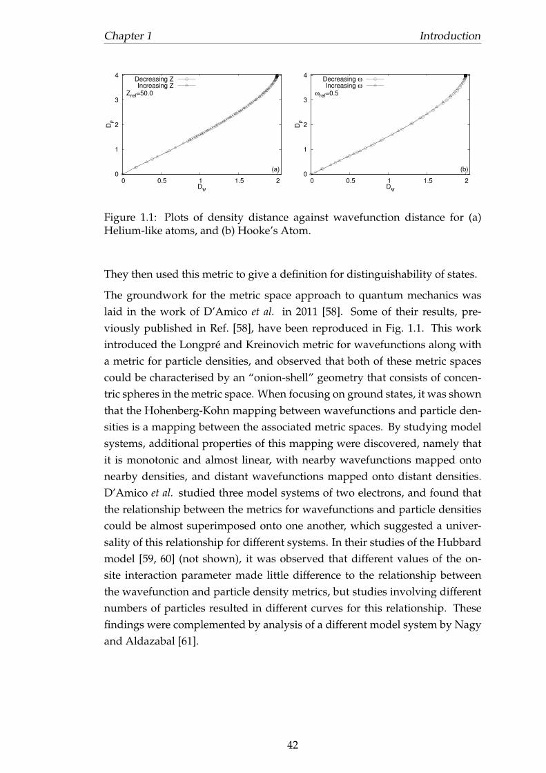
Figure 1.1: Plots of density distance against wavefunction distance for (a)Helium-like atoms, and (b) Hooke’s Atom.
They then used this metric to give a definition for distinguishability of states.
The groundwork for the metric space approach to quantum mechanics waslaid in the work of D’Amico et al. in 2011 [58]. Some of their results, pre-viously published in Ref. [58], have been reproduced in Fig. 1.1. This workintroduced the Longpre and Kreinovich metric for wavefunctions along witha metric for particle densities, and observed that both of these metric spacescould be characterised by an “onion-shell” geometry that consists of concen-tric spheres in the metric space. When focusing on ground states, it was shownthat the Hohenberg-Kohn mapping between wavefunctions and particle den-sities is a mapping between the associated metric spaces. By studying modelsystems, additional properties of this mapping were discovered, namely thatit is monotonic and almost linear, with nearby wavefunctions mapped ontonearby densities, and distant wavefunctions mapped onto distant densities.D’Amico et al. studied three model systems of two electrons, and found thatthe relationship between the metrics for wavefunctions and particle densitiescould be almost superimposed onto one another, which suggested a univer-sality of this relationship for different systems. In their studies of the Hubbardmodel [59, 60] (not shown), it was observed that different values of the on-site interaction parameter made little difference to the relationship betweenthe wavefunction and particle density metrics, but studies involving differentnumbers of particles resulted in different curves for this relationship. Thesefindings were complemented by analysis of a different model system by Nagyand Aldazabal [61].
42

Chapter 2
Introducing the Metric SpaceApproach to Quantum Mechanics
The axioms of a metric (1.61)–(1.63) are sufficiently general to allow a num-ber of valid metrics to be introduced for any set. Indeed, the discrete metric(1.72) is a metric for any non-empty set. The question that immediately arisestherefore is: which choice of metric is best for the set under consideration?
The metric space approach to quantum mechanics provides an answer to thisquestion for sets of quantum mechanical functions subject to conservation laws.The metric space approach involves deriving a metric that applies to the set offunctions subject to the conservation law from the law itself. Thus, we ensurethat the proposed metric stems from core characteristics of the systems anal-ysed and contains the related physics, and is therefore a “natural” metric forthe particular set of functions.
With the metric space approach to quantum mechanics, we have both a unifiedtheoretical grounding for the metrics for wavefunctions and particle densitiesintroduced in Refs. [57, 58], as well as a method to derive new metrics, whichwe apply to paramagnetic current densities and scalar potentials.
We published the general approach for deriving metrics presented in this chap-ter in Ref. [62], along with the paramagnetic current density metric. The dis-cussions of gauge theory with regard to the metrics was published in Ref. [63],and the metric for scalar potentials is ongoing research [64].
43

Chapter 2 Introducing the Metric Space Approach to Quantum Mechanics
2.1 Derivation of Metric Spaces from Conservation
Laws
In quantum mechanics, many conservation laws take the form∫| f (x)|p dx = c, (2.1)
for 0 < c < ∞. For each value of 16 p < ∞, the entire set of functions that satisfyEq. (2.1) belong to the Lp vector space, where the standard norm is the p-norm[51]
|| f (x)||p =[∫| f (x)|p dx
] 1p
. (2.2)
From any norm a metric can be introduced in a standard way via Eq. (1.82) sothat with p-norms we get
D f ( f1, f2) =
[∫| f1 (x)− f2 (x)|p dx
] 1p
. (2.3)
However before assuming this metric for the physical functions related to theconservation laws, an important consideration must be made: Eq. (2.3) hasbeen derived assuming the ensemble f to be a vector space; this is in factnecessary to introduce a norm. If we want to retain the metric (2.3), but re-strict it to the ensemble of physical functions satisfying Eq. (2.1), which doesnot necessarily form a vector space, we must show that Eq. (2.3) is a metric forthis restricted function set. This can be done using the general theory of metricspaces: given a metric space (X ,D) and S, a non empty subset of X , (S,D) is it-self a metric space with the metric D inherited from (X ,D). The metric axioms(1.61)–(1.63) automatically hold for (S,D) because they hold for (X ,D) [50, 51].Hence, we have a metric for the functions of interest, as their sets are non-empty subsets of the respective Lp sets.
This procedure can be extended to conservation laws of the form
n
∑i=1| fi|p = c, (2.4)
as the lp vector spaces for sums are directly analogous to the Lp spaces forintegrals [51]. In this case the induced metric will be
D f ( f1, f2) =
[n
∑i=1| f1i− f2i|
p
] 1p
. (2.5)
44

Chapter 2 Introducing the Metric Space Approach to Quantum Mechanics
Thus, we have a general procedure to construct a metric for any conservationlaw that is, or can be cast, in the form of Eq. (2.1) or Eq. (2.4).
Eqs. (2.3) and (2.5) are then the metrics that directly descend from the conserva-tion laws (2.1) and (2.4) respectively. Conversely any conservation law whichcan be recast as Eq. (2.1) (for example conservation of quantum numbers) orEq. (2.4) can be interpreted as inducing a metric on the appropriate, physicallyrelevant, subset of Lp or lp functions. This provides a general procedure toderive “natural” metrics from physical conservation laws. As they descenddirectly from conservation laws, these “natural” metrics are non-trivial andcontain the relevant physics.
2.2 Geometry of the Metric Spaces
Now that we have derived “natural” metrics from conservation laws, we canexamine the properties of these metrics. By considering spheres in the metricspaces, the geometry of the space can be determined. A sphere in a metricspace (X ,D) is the set of elements in the space that satisfy the condition
S(x0,r) = x ∈ X : D(x,x0) = r , (2.6)
where x0 is the centre and r is the radius of the sphere [51]. In order to con-struct our metric space geometry, we will consider the centre of a sphere to bethe zero function, i.e., f (0)(x)≡ 0. It can be seen that when we consider the dis-tance between the zero function and any other element in the metric space, werecover the p-norm, Eq. (2.2), defined from the conservation law, and therefore
the distance of any function from the zero function is one of a set of values c1pi .
A sphere of radius c1pi consists of all the functions which are conserved to the
same value ci. From this it can be seen that the conservation law has induced
a geometry consisting of a series of concentric spheres with radii c1pi , and cen-
tred at the zero function, forming an “onion-shell” geometry [58, 62]. This ispictorially shown in Fig. 2.1.
With the onion geometry in mind, we can find the extreme values that the met-ric (2.3) can take. When considering points on different spheres in the oniongeometry, the minimum value of the metric can be found from the reverse tri-angle inequality, Eq. (1.64),
D f ( fA, fB)>∣∣∣D f ( fA, f (0))−D f ( fB, f (0))
∣∣∣= ∣∣∣∣c 1pA − c
1pB
∣∣∣∣ . (2.7)
45

Chapter 2 Introducing the Metric Space Approach to Quantum Mechanics
c1/p1
c1/p2 c1/p
3
Figure 2.1: Sketch of the “onion-shell” geometry, consisting of a series of con-
centric spheres. The first three spheres are shown, with radii c1pi , i = 1,2,3.
This value is the difference in the radii of the two spheres representing fA andfB in the geometry. When considering the same sphere, we obtain an absoluteminimum value of zero, as required by axiom (1.61). The maximum valueof the metric for functions fA and fB is found from the triangle inequality,Eq. (1.63),
D f ( fA, fB)6 D f ( fA, f (0))+D f ( f (0), fB) = c1pA + c
1pB . (2.8)
On a single sphere in the geometry this reduces to 2c1p , which is the diameter
of the sphere. There is no absolute maximum for the metric in general becausethere is not necessarily an upper limit to the value of c, and therefore to thenumber of spheres in the onion geometry.
From the metric (2.3) and conditions in Eqs. (2.7) and (2.8), it can be seen thatmaximally distant functions are those which do not overlap at all and when
46
Chapter 2 Introducing the Metric Space Approach to Quantum Mechanics
the functions overlap exactly everywhere, i.e., they are the same function, theyare minimally distant [as required by axiom (1.61)]. Given this, we can inter-pret physically that the distance is inversely related to a measure of the spatialoverlap of the two functions.
2.3 Applying the Metric Space Approach to Quan-
tum Mechanical Functions
We now show how to apply the metric space approach to quantum mechanicsin order to obtain metrics for the fundamental quantities in DFT and CDFT.In order to do so, we will use the conservation laws derived in Sec. 1.1.2 toobtain metrics for paramagnetic current densities and scalar potentials, andshow how the metrics presented in recent literature for wavefunctions andparticle densities [57, 58] arise from their respective conservation laws.
2.3.1 Particle Densities
The particle density metric is derived from the conservation of the number ofparticles, Eq. (1.19), which can be written as∫
|ρ (r)|dr = N. (2.9)
Thus, as stated in Sec. 1.6.2, it can be seen that the particle density is an L1
function. Hence, the metric is given by [58]
Dρ (ρ1,ρ2) =∫|ρ1 (r)−ρ2 (r)|dr. (2.10)
From Eq. (2.9), it can be seen that the geometry of the particle density met-ric space consists of concentric spheres of radius N, such that the densities ofone-particle systems lie on a sphere of radius 1, two-particle densities lie on asphere of radius 2 and so on, as shown in Fig. 2.2.
2.3.2 Wavefunctions
In order to derive a metric for wavefunctions, we begin with the conservationof the norm of the wavefunction.
∫ ∣∣∣∣ψ (r,r2, . . . ,rN)√N
∣∣∣∣2 dr1 . . .drN = 1, (2.11)
47

Chapter 2 Introducing the Metric Space Approach to Quantum Mechanics
N=1N=2
N=3
Figure 2.2: The first three spheres of the “onion-shell” geometry for particledensities, with radii N = 1,2,3.
where we follow the convention of Refs. [58, 62] and normalise wavefunctionsto the particle number, N. This ensures that, rather than a single sphere repre-senting all wavefunctions, wavefunctions describing systems of different par-ticle numbers lie on different spheres in the “onion-shell” geometry and thusthe wavefunction metric space has a geometry similar to that for particle den-sities [58].
Equation (2.11) is of the form of Eq. (2.1), so following the procedure in Sec. 2.1we note that the wavefunction is an L2 function, and derive the metric
Dψ (ψ1,ψ2) =
[∫|ψ1−ψ2|2 dr1 . . .drN
] 12
, (2.12)
which is the standard Hilbert space metric [57]. However, as first noted byLongpre and Kreinovich [57], the metric (2.12) induced by the norm is not a
48

Chapter 2 Introducing the Metric Space Approach to Quantum Mechanics
sufficient measure of the distance between wavefunctions. This is because thedistance between the states ψ and ψ ′ = eiφ ψ , which differ only by a constantglobal phase factor, is non-zero. However, wavefunctions differing by sucha phase factor describe the same physics, as the solutions of the Schrodingerequation are only defined up to a constant global phase factor. To have physi-cally meaningful metrics, it is therefore important to define equivalence classessuch that the metric assigns zero distance to wavefunctions differing only by aconstant global phase factor.
An equivalence class for an element x ∈ X is defined as [65]
[x] =
x′ ∈ X : x∼ x′, (2.13)
where ∼ is the equivalence relation characterising the class. Each element ofthe set X belongs to a single equivalence class [65].
In order to account for an equivalence relation between elements, x∼ x′, we fol-low a general procedure for introducing an equivalence relation into a metricspace (X ,D). We define the following function [66]
D∼(x,y) = inf
k
∑i=1
D(pi,qi) : p1 = x,qk = y,k ∈ N
, (2.14)
where the infimum is taken over all choices of pi ,qi such that pi+1 ∼ qi.This implies that if x∼ y, D∼ (x,y) = D(x,x)+D(y,y) = 0 even if D(x,y) 6= 0 [66].This function is a semi-metric (or pseudometric) on the set X , known as thequotient semi-metric associated to the relation ∼. A semi-metric is a distancefunction that obeys all of the axioms of a metric except axiom (1.61): D(x,y) =
0 ⇐⇒ x = y, replacing it with: D(x,y) = 0 for x = y, i.e., we allow zero distancebetween non-identical elements as well as identical ones.
For Eq. (2.12) we have in general that Dψ
(ψ,eiφ ψ
)6= 0. If we introduce an
equivalence relation between wavefunctions differing by only a global phasefactor, and take k = 2 in Eq. (2.14), we find
Dψ (ψ1,ψ2) = inf
Dψ
(ψ1,ψ
′)+ Dψ (ψ2,ψ2), (2.15)
= inf
Dψ
(ψ1,ψ
′) , (2.16)
where ψ ′ = eiφ ψ2 ∼ ψ2 and we have used the positivity axiom of the metric.The choice of ψ ′ that will minimise the value of the semi-metric is determined
49

Chapter 2 Introducing the Metric Space Approach to Quantum Mechanics
by the phase factor, hence [57]
Dψ (ψ1,ψ2) = minφ
Dψ
(ψ1,eiφ
ψ2
). (2.17)
With this semi-metric space(ψ ,Dψ
), we can recover a metric space in a nat-
ural way, by “gluing” equivalent elements to form a set of equivalence classes.By considering the set of equivalence classes of wavefunctions, rather thanthe set of all wavefunctions, wavefunctions differing only by a constant globalphase factor are identified with one another. Thus, the set of equivalent wave-functions with Dψ is a metric space, with the metric defined between each ofthe equivalence classes, as required [65].
Longpre and Kreinovich showed that we do not need to perform this minimi-sation explicitly, and instead we can simplify the metric (2.17) by writing [57]
Dψ = minφ
[∫ ∣∣∣ψ1− eiφψ2
∣∣∣2 dr1 . . .drN
] 12
,
= minφ
[∫ (ψ1− eiφ
ψ2
)∗(ψ1− eiφ
ψ2
)dr1 . . .drN
] 12
,
= minφ
[∫ (ψ∗1 − e−iφ
ψ∗2
)(ψ1− eiφ
ψ2
)dr1 . . .drN
] 12
,
= minφ
[∫ (ψ∗1 ψ1 +ψ
∗2 ψ2− eiφ
ψ∗1 ψ2− e−iφ
ψ∗2 ψ1
)dr1 . . .drN
] 12
,
= minφ
[∫|ψ1|2 + |ψ2|2 dr1 . . .drN−
∫eiφ
ψ∗1 ψ2dr1 . . .drN−
∫e−iφ
ψ∗2 ψ1dr1 . . .drN
] 12
,
= minφ
[∫|ψ1|2 + |ψ2|2 dr1 . . .drN−
∫eiφ
ψ∗1 ψ2dr1 . . .drN−
(∫eiφ
ψ2ψ∗1 dr1 . . .drN
)∗] 12
,
= minφ
[∫|ψ1|2 + |ψ2|2 dr1 . . .drN−2Re
(∫eiφ
ψ∗1 ψ2dr1 . . .drN
)] 12
.
It can now be seen that the distance is at a minimum when the real part of∫eiφ ψ∗1 ψ2dr1 . . .drN is at a maximum.
For any complex number, z,
|z|2 = Re(z)2 + Im(z)2.
Since Im(z)2 is always positive,
|z|2 > Re(z)2 =⇒ |z|> |Re(z)|> Re(z),
50

Chapter 2 Introducing the Metric Space Approach to Quantum Mechanics
so it can be seen that the real part of any complex number is at a maximumwhen it is equal to the magnitude of the complex number.
This allows us to write the wavefunction metric as [57, 58, 62]
Dψ (ψ1,ψ2) =
[∫|ψ1|2 + |ψ2|2 dr1 . . .drN−2
∣∣∣∣∫ ψ∗1 ψ2dr1 . . .drN
∣∣∣∣] 12
, (2.18)
which is the form we use.
2.3.2.1 Orthogonal Wavefunctions
The term∫
ψ∗1 ψ2dr1 . . .drN in the wavefunction metric (2.18) shows a connec-tion between the wavefunction metric and the Born Rule of quantum mechan-ics [6], which, as discussed in Chapter 1, interprets the wavefunction as a sta-tistical quantity, such that |ψ (r)|2 dr represents the probability of finding a par-ticle within the volume element dr [1].
To consider the Born Rule for two different wavefunctions, φ and ψ , we expandφ in the complete set of eigenfunctions of a Hermitian operator O, φ = ∑n cnφn.The Born Rule states that the inner product of the one of the eigenfunctions φn
with ψ represents the probability of measuring the state ψ with the operatorO and obtaining the eigenvalue corresponding to the eigenstate φn. In the casethat 〈φn | ψ〉 = 0, the wavefunctions are orthogonal, and represent mutuallyexclusive physical states [1, 67].
The principal consequence of this with regards to the wavefunction metricis that whenever two wavefunctions ψ1 and ψ2 are orthogonal, they will al-ways be assigned the maximum distance by the wavefunction metric, whichis√
N1 +N2, where Ni is the number of particles in the system described by thestate ψi. This point was first raised by Artacho [68, 69] with regards to wave-functions corresponding to systems of different numbers of particles, but alsoapplies in any other situation where wavefunctions are orthogonal, for exam-ple, when considering a ground state and an excited state of the same system.
For the case of systems of different particle numbers, the wavefunction met-ric (2.18) will always assign their wavefunctions as maximally distant. For thisreason, we restrict our use of the the metric (2.18) to systems with the samenumber of particles, N.
51

Chapter 2 Introducing the Metric Space Approach to Quantum Mechanics
√N√2N
Figure 2.3: A sphere of the “onion-shell” geometry for wavefunctions, withradius
√N and maximum value
√2N.
2.3.2.2 Geometry of the Metric Space
Writing the metric in the form of Eq. (2.18) has interesting consequences for the“onion-shell” geometry of the wavefunction metric space [58]. From Eq. (2.8),it can be seen that the maximum distance between two N-particle wavefunc-tions is 2
√N, which corresponds to the maximum value obtained when writing
the wavefunction metric in the form of Eq. (2.12). However, it can be seen thatthe maximum value of the metric (2.18) is obtained for orthogonal wavefunc-tions, and is
√2N < 2
√N.
As far as the “onion-shell” geometry is concerned, we can find the angle be-
52

Chapter 2 Introducing the Metric Space Approach to Quantum Mechanics
tween two wavefunctions with a distance of√
2N from the cosine rule,
cosθ =
(√N)2
+(√
N)2−2
(√N)2
2(√
N)2 = 0 ⇒ θ =
π
2, (2.19)
i.e., one wavefunction is located halfway around the sphere from the other. Inother words, if we consider an arbitrary wavefunction to lie on the north poleof the sphere, a wavefunction that is maximally distant, according to Eq. (2.18),lies on the equator. This is shown in Fig 2.3.
2.3.3 Paramagnetic Current Densities
In Ref. [62] we derived a metric for the paramagnetic current density, jp (r). Inorder to apply the metric space approach to generate a metric for the param-agnetic current density, we must first relate it to a conservation law of the formof Eq. (2.1). We will show that the paramagnetic current density obeys∫
[r× jp (r)]z dr = 〈ψ | Lz |ψ 〉 , (2.20)
where Lz is defined as in Eq. (1.20), and jp (r) =⟨jp⟩. The form of the paramag-
netic current density operator is [7]
jp =12
N
∑i=1
[δ (r− ri) pri + priδ (r− ri)] . (2.21)
The expectation value of r× jp is,
⟨r× jp
⟩=〈ψ (r1,r2, . . . ,rN) |r× jp |ψ (r1,r2, . . . ,rN)〉 ,
=12
N
∑i=1
∫ ∫. . .∫
ψ∗ (r1,r2, . . . ,rN) [r×δ (r− ri) pri]ψ (r1,r2, . . . ,rN)dr1dr2 . . .drN
+∫ ∫
. . .∫
ψ∗ (r1,r2, . . . ,rN) [r× priδ (r− ri)]ψ (r1,r2, . . . ,rN)dr1dr2 . . .drN
,
=12
N
∑i=1
∫ ∫. . .∫
ψ∗ (r1,r2, . . . ,rN)δ (r− ri) [r× pri]ψ (r1,r2, . . . ,rN)dr1dr2 . . .drN
+∫ ∫
. . .∫
ψ∗ (r1,r2, . . . ,rN) [r× pri]δ (r− ri)ψ (r1,r2, . . . ,rN)dr1dr2 . . .drN
.
53

Chapter 2 Introducing the Metric Space Approach to Quantum Mechanics
We rewrite the second integral by noting that the operators r× pri and δ (r− ri)
are both Hermitian. Therefore, we can apply the relation [8],
〈φ | AB |ψ 〉= 〈φ | BA |ψ 〉∗ . (2.22)
This gives,
⟨r× jp
⟩=
12
N
∑i=1
∫ ∫. . .∫
ψ∗ (r1,r2, . . . ,rN)δ (r− ri) [r× pri]ψ (r1,r2, . . . ,rN)dr1dr2 . . .drN
+∫ ∫
. . .∫
ψ (r1,r2, . . . ,rN)δ (r− ri) [r× pri]∗
ψ∗ (r1,r2, . . . ,rN)dr1dr2 . . .drN
.
We now have a series of 2N N-dimensional integrals. The delta function re-moves one integral from each term in this series, resulting in 2N N−1-dimensionalintegrals. By renaming each set of dummy variables as r2 . . .rN , we have,
⟨r× jp
⟩=
12
N
∑i=1
∫. . .∫
ψ∗ (r,r2, . . . ,rN) [r× pr]ψ (r,r2, . . . ,rN)dr2 . . .drN
+∫
. . .∫
ψ (r,r2, . . . ,rN) [r× pr]∗
ψ∗ (r,r2, . . . ,rN)dr2 . . .drN
.
Integrating over r gives
∫ ⟨r× jp
⟩dr =
12
N
∑i=1
∫ ∫. . .∫
ψ∗ (r,r2, . . . ,rN) [r× pr]ψ (r,r2, . . . ,rN)dr2 . . .drN
+∫
. . .∫
ψ (r,r2, . . . ,rN) [r× pr]∗
ψ∗ (r,r2, . . . ,rN)dr2 . . .drN
dr.
(2.23)
Since the vector r is independent of the coordinates (r2 . . .rN), and the crossproduct is a linear operation, we can remove the vector r from the integralsover the coordinates (r2 . . .rN),
∫ ⟨r× jp
⟩dr =
12
N
∑i=1
∫r×∫
. . .∫
ψ∗ (r,r2, . . . ,rN) prψ (r,r2, . . . ,rN)dr2 . . .drN
+∫
. . .∫
ψ (r,r2, . . . ,rN) p∗r ψ∗ (r,r2, . . . ,rN)dr2 . . .drN
dr,
=∫
r×− i2
N
∑i=1
∫. . .∫
ψ∗ (r,r2, . . . ,rN)∇rψ (r,r2, . . . ,rN)dr2 . . .drN
−∫
. . .∫
ψ (r,r2, . . . ,rN)∇rψ∗ (r,r2, . . . ,rN)dr2 . . .drN
dr,
=∫
r× jp (r)dr.
54

Chapter 2 Introducing the Metric Space Approach to Quantum Mechanics
Returning to Eq. (2.23), and noting that r× pr is Hermitian,
∫ ⟨r× jp
⟩dr =
12
N
∑i=1
∫ ∫. . .∫
ψ∗ (r,r2, . . . ,rN) [r× pr]ψ (r,r2, . . . ,rN)dr2 . . .drN
+∫
. . .∫
ψ∗ (r,r2, . . . ,rN) [r× pr]ψ (r,r2, . . . ,rN)dr2 . . .drN
dr,
=∫ N
∑i=1
∫. . .∫
ψ∗ (r,r2, . . . ,rN) [r× pr]ψ (r,r2, . . . ,rN)dr2 . . .drNdr,
=∫ ∫
. . .∫ N
∑i=1
ψ∗ (r,r2, . . . ,rN) [r× pr]ψ (r,r2, . . . ,rN)drdr2 . . .drN ,
=⟨L⟩.
We have thus proved that∫ ⟨r× jp
⟩dr =
⟨L⟩=∫
[r× jp (r)]dr. (2.24)
Since Eq. (2.24) applies to the vectors [r× jp (r)] and L, it must also apply toeach component of these vectors, hence∫
[r× jp (r)]z dr =⟨Lz⟩= m, (2.25)
provided that Lz is a constant of motion. In order to turn Eq. (2.25) into aconservation law of the form of Eq. (2.1), we note that m can be any positiveor negative integer, hence we take the absolute value to ensure that the finalconstant is positive, ∣∣∣∣∫ [r× jp (r)]z dr
∣∣∣∣= ∣∣⟨Lz⟩∣∣= |m| . (2.26)
Provided that [r× jp (r)]z has the same sign everywhere, which applies whenthe system under consideration is rotationally invariant about the z axis (i.e.,jp (r) has no θ dependence), we can write,∫ ∣∣[r× jp (r)]z
∣∣dr = |m| , (2.27)
giving us the form of conservation law required. From this, we can now followour procedure and derive the metric,
Djp⊥(jp1, jp2) =
∫ ∣∣∣r× [jp1 (r)− jp2 (r)]
z
∣∣∣dr. (2.28)
The radii of the concentric spheres in the “onion-shell” geometry for the para-
55

Chapter 2 Introducing the Metric Space Approach to Quantum Mechanics
magnetic current density metric space are |m|, with the paramagnetic currentdensities located on the spheres corresponding to the value of |m| given byEq. (2.25).
As we take the z-component of the cross product in the paramagnetic cur-rent density metric (2.28), it is clear that the z-component of the paramag-netic current density itself does not affect the value of the metric. Therefore,Djp⊥
is a distance between equivalence classes of paramagnetic currents, eachclass characterized by current densities having the same transverse componentjp⊥ ≡ ( jpx , jpy).
It transpires that a metric for the transverse components of the current den-sity is well suited for studying systems subject to longitudinal magnetic fields.Classically, it is well known that a particle moving in a magnetic field experi-ences the Lorentz force, which is given by [12]
F = E+1c
v×B, (2.29)
where F is the force, v is the velocity and E and B are the electric and magneticfields. By virtue of the cross product in Eq. (2.29), the particle experiences aforce perpendicular to the direction of the magnetic field, which will act toinduce motion in the plane transverse to direction of the field.
Quantum mechanically, the physical current density is given by [7],
j(r) =12
N
∑i=1
δ (r− ri)
[pri +
1c
A(ri)
]+
[pri +
1c
A(ri)
]δ (r− ri)
. (2.30)
The physical current density can be written as a superposition of transverseand longitudinal components,
j(r) = jT (r)+ jL (r) , (2.31)
where the components are defined by the identities,
∇ · jT (r) = 0, ∇× jL (r) = 0. (2.32)
We can also split the vector potential, A(r), into transverse and longitudinalcomponents obeying the same identities,
A(r) = AT (r)+AL (r) , ∇ ·AT (r) = 0, ∇×AL (r) = 0. (2.33)
We can see immediately from Eq. (2.33) that the longitudinal component ofthe vector potential cannot contribute to the magnetic field. Therefore, the
56

Chapter 2 Introducing the Metric Space Approach to Quantum Mechanics
magnetic field is entirely captured by the transverse component of the vectorpotential. Thus, changes in the magnetic field correspond to changes in thetransverse component of the vector potential, which is captured in the trans-verse component of the physical current density.
2.3.4 Scalar Potentials
For scalar potentials, we consider the conservation of energy, Eq. (1.25), in or-der to derive a metric [64]. The expectation value of the Hamiltonian is∫ ∫
. . .∫
ψ∗ (r,r2, . . . ,rN) Hψ (r,r2, . . . ,rN)dr1dr2 . . .drN = E. (2.34)
In order to ensure that the resulting metric will satisfy the positivity axiom(1.61), we must take the absolute value of the energy,∣∣∣∣∫ ∫ . . .
∫ψ∗ (r,r2, . . . ,rN) Hψ (r,r2, . . . ,rN)dr1dr2 . . .drN
∣∣∣∣= |E| . (2.35)
To derive a non-trivial metric, we must ensure that the conservation law is ofthe form of Eq. (2.1), i.e., be able to “move” the absolute value signs inside theintegral, taking the absolute value of the integrand. This can be done only ifthe integrand always has the same sign throughout its domain. Writing theHamiltonian explicitly, we have:
∫ ∫. . .∫
ψ∗
N
∑i=1
[−∇2
i2
+∑j<i
1∣∣ri− r j∣∣ +V (ri)
]ψdr1dr2 . . .drN = E
∫ ∫. . .∫ N
∑i=1
[−ψ∗∇2
i ψ
2+∑
j<i
|ψ|2∣∣ri− r j∣∣ + |ψ|2V (ri)
]dr1dr2 . . .drN = E (2.36)
where the three terms on the left hand side correspond to the kinetic energy,the energy of the Coulomb interaction between the electrons and the potentialenergy respectively. We will now demonstrate that each of the terms in theintegrand can be written such that they are positive semidefinite everywhere.The integrand of the Coulomb term clearly satisfies this requirement already,so we need only consider the remaining two terms.
2.3.4.1 Kinetic Energy
The kinetic energy of the ith particle is given by
T =−12
∫ψ∗ (r,r2, . . . ,rN)∇
2i ψ (r,r2, . . . ,rN)dr1dr2 . . .drN . (2.37)
57

Chapter 2 Introducing the Metric Space Approach to Quantum Mechanics
Writing this integral explicitly gives:
−12
∫ψ∗∇
2i ψdri =−
12
∫∞
0
∫π
0
∫ 2π
0
(ψ∗∇
2i ψ)
r2i sinθidridθidφi,
=−12
∫∞
0
∫π
0
∫ 2π
0ψ∗[
1r2
i
∂
∂ ri
(r2
i∂ψ
∂ ri
)+
1r2
i sinθi
∂
∂θi
(sinθi
∂ψ
∂θi
)+
1r2
i sin2θi
∂ 2ψ
∂φ 2i
]r2
i sinθidridθidφi.
Taking each of the three terms in turn, we will perform integration by partsin order to rewrite the kinetic energy. For the first term, we will evaluate theradial integral by parts,
−12
∫∞
0ψ∗[
1r2
i
∂
∂ ri
(r2
i∂ψ
∂ ri
)]r2
i dri =−12
[r2
i ψ∗∂ψ
∂ ri
]∞
0+
12
∫∞
0r2
i
(∂ψ∗∂ ri
∂ψ
∂ ri
)dri,
=12
∫∞
0
∣∣∣∣∂ψ
∂ ri
∣∣∣∣2r2i dri,
where we have used that ψ → 0 as ri→ ∞. For the second term, we calculatethe θ integral by parts,
−12
∫π
0ψ∗[
1r2
i sinθi
∂
∂θi
(sinθi
∂ψ
∂θi
)]sinθidθi =−
12
[ψ∗
r2i
sinθi∂ψ
∂ ri
]π
0
+12
∫π
0
1r2
isinθi
(∂ψ∗∂θi
∂ψ
∂θi
)dθi,
=12
∫π
0
∣∣∣∣ 1ri
∂ψ
∂θi
∣∣∣∣2 sinθidθi.
Finally, we perform the φ integral by parts for the third term,
−12
∫ 2π
0ψ∗
[1
r2i sin2
θi
∂ 2ψ
∂φ 2i
]dφi =−
12
[ψ∗
r2i sin2
θi
∂ψ
∂φi
]2π
0
+12
∫ 2π
0
1r2
i sin2θi
(∂ψ∗∂φi
∂ψ
∂φi
)dφi,
=12
∫ 2π
0
∣∣∣∣ 1ri sinθi
∂ψ
∂φi
∣∣∣∣2 dφi,
where we use the fact that the wavefunction and its derivatives must be con-tinuous in order to eliminate the first term.
58

Chapter 2 Introducing the Metric Space Approach to Quantum Mechanics
Therefore, for the full integral, we have,
−12
∫ψ∗∇
2i ψdri =
12
∫∞
0
∫π
0
∫ 2π
0
[∣∣∣∣∂ψ
∂ ri
∣∣∣∣2 + ∣∣∣∣ 1ri
∂ψ
∂θi
∣∣∣∣2 + ∣∣∣∣ 1ri sinθi
∂ψ
∂φi
∣∣∣∣2]
r2i sinθidridθidφi,
=12
∫|∇ψ|2 dri,
and the kinetic energy is given by
T =12
∫ ∫. . .∫|∇ψ|2 dr1dr2 . . .drN . (2.38)
Thus, the integrand of the kinetic energy term is positive semidefinite every-where.
2.3.4.2 Potential Energy
The potential energy is given by
V =N
∑i=1
∫ ∫. . .∫
ψ∗ (r,r2, . . . ,rN)V (ri)ψ (r,r2, . . . ,rN)dr1dr2 . . .drN , (2.39)
where V (ri) is defined by the system under consideration. Although we can-not guarantee the sign of V (ri), we can make use of a gauge transformation.If the potential is modified by a constant, V (ri)→ V (ri)+ c, then the solutionto the Schrodinger equation is unaffected. Thus, when considering potentialsthat have a single minimum, we can choose a constant c such that the valueof the integrand is positive everywhere for all of the potentials that we con-sider. Hence, when studying systems with the potential metric, we must al-ways work in the same gauge and that gauge must be chosen in order to allowthe expectation value of the Hamiltonian to be written as a well-defined norm.This approach works well for potentials with a single minimum, but we areaware of some cases where more care must be taken in order to ensure that thepotential metric gives physically relevant results.
2.3.4.3 Forming the Potential Metric
Our expectation value is now given by
∫ ∫. . .∫ N
∑i=1
[12|∇ψ|2 +∑
j<i
ψ∗ψ∣∣ri− r j∣∣ +ψ
∗ [V (ri)+ c]ψ
]dr1dr2 . . .drN = E + c,
59

Chapter 2 Introducing the Metric Space Approach to Quantum Mechanics
and we can write∣∣∣∣∣∫ ∫
. . .∫ N
∑i=1
[12|∇ψ|2 +∑
j<i
ψ∗ψ∣∣ri− r j∣∣ +ψ
∗ [V (ri)+ c]ψ
]dr1dr2 . . .drN
∣∣∣∣∣= |E + c| ,
∫ ∫. . .∫ ∣∣∣∣∣ N
∑i=1
[12|∇ψ|2 +∑
j<i
ψ∗ψ∣∣ri− r j∣∣ +ψ
∗ [V (ri)+ c]ψ
]∣∣∣∣∣dr1dr2 . . .drN = |E + c| ,∫ ∫. . .∫ ∣∣H ′∣∣dr1dr2 . . .drN =
∣∣E ′∣∣ , (2.40)
where E ′ = E + c. Hence, we derive the following metric,
DV =∫ ∫
. . .∫ ∣∣H ′1− H ′2
∣∣dr1dr2 . . .drN (2.41)
with spheres of radii E ′ for the “onion-shell” geometry. It can be seen thatthis metric can be applied to the potential, rather than the whole Hamiltonian,by considering each of the terms in H ′. All of the terms contain the manybody wavefunction, ψ (r,r2, . . . ,rN); from the Schrodinger equation, the manybody wavefunction can be seen to be defined uniquely by the external poten-tial V (r). Hence, we can write,
ψ = ψ [V (r)] . (2.42)
In DFT, it is sometimes stated that T and U are universal functionals of thedensity. This is because, assuming the nature of the interaction between theelectrons is fixed, T and U are identical for all systems - where a system isprescribed by the external potential [3]. Applying a similar argument to thepotential metric allows us to write Eq. (2.40) as
∫ ∫. . .∫ ∣∣∣∣∣ N
∑i=1
[F [V ]+ψ∗ [V (ri)+ c]ψ]
∣∣∣∣∣dr1dr2 . . .drN = |E + c| , (2.43)
where F [V ] is a functional of the potential analogous to the DFT universalfunctional F [ρ].
2.3.4.4 A Note on Coulomb Potentials
An important class of systems studied in quantum mechanics are atomic-likesystems, where the external potential is of the form of − 1
rifor each particle. At
first glance, this causes a problem with the argument in Sec. 2.3.4.2, because ifV (0) = −∞ and ψ (0) 6= 0, then it is impossible for a gauge transformation toenable the integrand of the potential norm, given by Eq. (2.40), to be positiveeverywhere.
60

Chapter 2 Introducing the Metric Space Approach to Quantum Mechanics
However, in two dimensions, dri = ridri, and in three dimensions, dri = r2i sinθdri.
Hence, the factors of ri in the Jacobean determinant cancel with the factor of ri
in the potential, resulting in the potential energy term being finite and, there-fore, amenable to a gauge transformation provided we study the system inat least two dimensions. In one-dimensional modelling of quantum systems,Coulomb potentials are typically replaced by softened potentials that are finiteat ri = 0 [70, 71].
2.4 Gauge Theory
In this thesis, we will consider systems subject to magnetic fields. When deal-ing with electromagnetic fields, it is important to consider the choice of gauge.The scalar and vector potentials in the Hamiltonian (1.5) are not unique, as achange of gauge transforms the potentials according to:
V ′ (r) =V (r)+ c, A′ (r) = A(r)−∇χ, (2.44)
where c is a constant and χ (r) is a scalar field [39]. These transformationspreserve the electromagnetic fields and all physical observables.
With regard to the quantities we have considered in this chapter, the particledensity is gauge invariant, but the wavefunction, paramagnetic current den-sity and scalar potential are not. After a change of gauge, the wavefunctionundergoes a unitary transformation, which is given by [72]
ψ′ (r) = e[iχ(r)]ψ (r) . (2.45)
The paramagnetic current density transforms according to [39]
j′p (r) = jp (r)+ρ (r)∇χ. (2.46)
Thus, when considering changes in the vector potential, we must be aware ofthe effect of gauge transformations on the physical quantities we are consid-ering. Our metrics are constructed to provide non-trivial information that isphysically relevant, since they are based on conservation laws. It is paramountthen that they are also gauge invariant.
For wavefunctions, a gauge transformation introduces a global phase factor.In Sec. 2.3.2, we defined all wavefunctions differing only by a constant globalphase as equivalent and wrote the wavefunction metric in the form of Eq. (2.18).This has ensured that the wavefunction metric is gauge invariant. We now
61

Chapter 2 Introducing the Metric Space Approach to Quantum Mechanics
consider the effect of gauge theory for the paramagnetic current density met-ric [63].
2.4.1 Gauge Invariance for the Paramagnetic Current Density
Metric
In Ref. [63], we analysed the paramagnetic current density metric in differentgauges. In order to consider the gauge properties of Djp⊥
(jp1, jp2), first of all werequire that jp1 and jp2 are within the same gauge. Then, applying the gaugetransformation in Eq. (2.46) we obtain
Djp⊥
(j′p1
, j′p2
)=∫ ∣∣∣r×
[j′p1
(r)− j′p2(r)]
z
∣∣∣dr,
=∫ ∣∣∣(r×jp1 (r)− jp2 (r)+ [ρ1 (r)−ρ2 (r)]∇χ
)z
∣∣∣dr. (2.47)
Equation (2.47) states that, in general, the paramagnetic current density dis-tance defined by Eq. (2.28) is modified by a gauge transformation. This seemsto contradict the fact that we base our metrics on conservation laws, whichmust be gauge invariant. In order to reconcile this apparent contradiction letus explore more closely which quantities are gauge variant and which are theones that must be conserved.
With reference to Eq. (2.25), the measurable physical quantity which must beconserved by gauge transformations is m, which, in the gauge chosen, corre-sponds to the component Lz of the angular momentum. However it is crucialto note that Lz is not (nor need be) gauge invariant.
The operator Lz is defined in Eq. (1.20) as the cross product of r and the canon-ical linear momentum, p. Although r is gauge invariant, p is gauge variant,and therefore, so is Lz. In the following we wish to extend Eq. (2.28) so that themetric associated to the conservation of m is indeed gauge invariant.
We consider a system for which there exists at least one gauge such that [Lz, H] =
0, with H the system Hamiltonian. We name this the reference gauge and re-fer to its vector potential as Are f (r) and to its paramagnetic current density asjpre f (r). In this reference gauge the set m corresponds to the eigenvalues of Lz
and both equalities in the relation (2.25) hold. The set m are then constantsof motion, and in this gauge they represent the z-component of the angularmomentum, Lz.
We now focus on the generic gauge corresponding to a generic vector potentialA(r). In this generic gauge, the first equality of Eq. (2.25) holds, but the secondequality holds only if Lz is a constant of motion in this gauge.
62

Chapter 2 Introducing the Metric Space Approach to Quantum Mechanics
We will now consider the quantity
jp (r)≡ jp (r)−ρ (r)∇χre f (2.48)
and the operator
Lz ≡N
∑i=1
[r×(p−∇χre f
)]z , (2.49)
where ∇χre f is defined by A = Are f −∇χre f . We note that jp (r) is gauge invari-ant, as, from equation (2.46),
jp (r)≡ jpre f (r) (2.50)
always. It follows that ∫ [r× jp (r)
]zdr = m, (2.51)
independently of the gauge. Furthermore, by using the definition (2.48), and thefirst equality of Eq. (2.25), which holds regardless of whether or not Lz is aconstant of motion, we obtain∫ [
r× jp (r)]
zdr = 〈ψ | Lz |ψ 〉−
∫ [r×ρ (r)∇χre f
]z dr,
= 〈ψ | Lz |ψ 〉−〈ψ |(r×∇χre f
)z |ψ 〉 ,
= 〈ψ | Lz |ψ 〉 . (2.52)
This demonstrates that equation (2.49) defines the operator associated to theconservation law (2.51), independently of the gauge. In particular, compar-ison of Eq. (2.51) and Eq. (2.52) shows that indeed Lz is the operator whoseeigenvalues are m independently of the gauge.1
Lz reduces to Lz in the reference gauge, and in all gauges where Lz is a constantof motion, as should be expected. This is because the limited set of gaugesfor which
[Lz, H
]= 0 holds, is the same within which both Lz and [r× jp (r)]z
are unaffected by gauge transformations. These gauges correspond to vectorpotentials of the form of Eq. (1.22). These vector potentials are linked by gaugetransformations of the form χ
(x2 + y2,z
). The proofs of these statements are
given in Appendices A and B respectively.
1We note that Lz is related to the gauge invariant z component of the moment of mechanicalmomentum Kz = Lz +[r×A(r)]z as Lz = Kz−
(r×Are f
)z, but that Kz would not be a constant of
motion in all gauges, that is, its eigenvalues are generally different from m. Likewise jp (r)does not coincide with the gauge invariant total current density j(r) = jp (r)+ρ (r)A(r).
63
Chapter 3
Applying the Metric SpaceApproach to Current DensityFunctional Theory
For systems subject to a vector potential with a Hamiltonian of the form ofEq. (1.5), CDFT states that the ground state wavefunction obtained from theSchrodinger equation is uniquely defined by the particle density and the para-magnetic current density taken together, and vice versa [39, 40]. Equations (1.18)and (1.54) clearly demonstrate how each of the densities are obtained from thewavefunction. However, no suggestion on the details of the map from thebasic densities to the wavefunction is offered by either Hohenberg and Kohnwith regards to standard DFT, or Vignale and Rasolt for CDFT.
The metric space approach to quantum mechanics allows us to explore thisunique relationship, comparing the distances between wavefunctions to thedistances between their corresponding particle densities and their correspond-ing paramagnetic current densities. Building on the analysis for standard DFTin Ref. [58], we will consider model systems, for which we can generate highlyaccurate solutions, and calculate the wavefunctions, particle densities and para-magnetic current densities for a range of Hamiltonians. Comparing the dis-tances between corresponding quantities will enable us to build up a pictureof the unique relationship at the core of CDFT. The results in this chapter thatrelate to varying the confinement potential were published in Ref. [62].
64

Chapter 3 Applying the Metric Space Approach to CDFT
3.1 Model Systems
In this Chapter, and the next, we will consider two model systems: the mag-netic Hooke’s Atom, and the Inverse Square Interaction System. Both of theseare two-dimensional systems, immersed in a magnetic field that is applied per-pendicular to the plane of confinement.
3.1.1 Magnetic Hooke’s Atom
Hooke’s Atom is a system consisting of two electrons confined in a harmonicoscillator potential. It is particularly notable as one of few examples of quan-tum many-body systems for which exact solutions exist [73, 74]. Analyticalsolutions also exist when the system is subject to a magnetic field. The Hamil-tonian in this case, in atomic units, is given by [42, 75]
H =2
∑i=1
12
[pi +
1c
A(ri)
]2
+12
ω20 r2
i
+
1|r2− r1|
(3.1)
where ω0 is the harmonic confinement frequency and c is the speed of light.We introduce centre of mass and relative motion coordinates, defined as,
R =12(r1 + r2) , r = r2− r1. (3.2)
This allows us to define the momentum operators,
pR = p1 +p2, pr =12(p2−p1) , (3.3)
and the vector potentials,
AR (R) =12[A(r1)+A(r2)] , Ar (r) = A(r2)−A(r1) . (3.4)
We will study the system in two dimensions, and work in cylindrical coor-dinates with the magnetic field applied perpendicular to the plane such thatB = Bz [42, 75].
In centre of mass and relative motion coordinates, we have
H = 2
[12
(pr +
12c
Ar (r))2
+18
ω20 r2 +
12r
]+
12
[12
(pR +
2c
AR (R)
)2
+2ω20 R2
].
(3.5)It can be seen that the Hamiltonian is separable into relative motion and cen-tre of mass components. The centre of mass Hamiltonian is simply that of a
65
Chapter 3 Applying the Metric Space Approach to CDFT
single particle harmonic oscillator subject to a magnetic field, which is treatedin Refs. [76–78]. Writing the centre of mass wavefunction as ξ (R) = eiMθU (R),the Schrodinger equation reduces to [77]
d2UdR2 +
1R
dUdR−M2
R2 U (R)− ω2r2U (R) = 2
(η− mωc
4
)U (R) , (3.6)
where η is the centre of mass energy and M is the angular momentum quantumnumber for the centre of mass. The frequency ω is the effective frequency ofthe harmonic oscillator, which we define using Taut’s convention [42, 75] as,
ω =
√ω2
0 +(
ωc
2
)2, (3.7)
where ωc =Bc is the cyclotron frequency. The solution for the centre of mass
is [75],ξ (R) = (2ωR)|M| eiMθ L|M|N
(2ωR2)e−ωR2
, (3.8)
where L|M|N are associated Laguerre polynomials [20, 79], N = 0,1,2, . . . and M =
0,±1,±2, . . . ,±N.
The centre of mass energy is given by [75],
η = (2N +1+ |M|) ω +Mωc
2. (3.9)
For the ground state, N = M = 0, so η = ω and the normalised ground statewavefunction is
ξ0 (R) =
√2ω
πe−ωR2
. (3.10)
Turning our attention to the relative motion, we expand the Hamiltonian andchoose the symmetric gauge, Ar (r) = 1
2B× r = 12Brθ , which is of the form of
Eq. (1.22). The time-independent Schrodinger equation reads,[12
(−i∇r +
12c
Ar (r))2
+18
ω20 r2 +
12r
]φ (r) =
ε
2φ (r) , (3.11)
which can be expanded as,
12
[−∇
2r φ − i
2c(φ∇ ·Ar (r)+2Ar (r) ·∇φ)+
A2r
4c2 φ
]+
18
ω20 r2
φ +12r
φ =ε
2φ ,
From our choice of gauge, we know that ∇ ·Ar (r) = 0. Expanding the remain-
66

Chapter 3 Applying the Metric Space Approach to CDFT
ing vector operations gives,
12
[−∂ 2φ
∂ r2 −1r
∂φ
∂ r− 1
r2∂ 2φ
∂θ 2 −iωc
2∂φ
∂θ+
116
ω2c r2
φ
]+
18
ω20 r2
φ +12r
φ =ε
2φ ,
12
[− 1√
r∂ 2
∂ r2
(√rφ)− 1
4r2 φ − 1r2
∂ 2φ
∂θ 2 −iωc
2∂φ
∂θ+
116
ω2c r2
φ
]+
18
ω20 r2
φ +12r
φ =ε
2φ .
(3.12)
At this point, Taut writes the ansatz [42, 75],
φ (r) =eimθ
√2π
u(r)√r
m = 0,±1,±2, . . . , (3.13)
where m is the quantum number corresponding to the z-component of the an-gular momentum for the relative motion. This ansatz reduces Eq. (3.12) to
− 12
[d2
dr2 u(r)+1
4r2 u(r)− m2
r2 u(r)− 12
mωcu(r)− 116
ω2c r2u(r)
]+
18
ω20 r2u(r)+
12r
u(r) =ε
2u(r) ,
− 12
d2
dr2 u(r)+1
2r2
(m2− 1
4
)u(r)+
18
ω2r2u(r)+
12r
u(r) =(
ε
2− 1
4mωc
)u(r) .
(3.14)
As r → ∞, the system will tend towards that of two isolated single-particleharmonic oscillators. Therefore, we write
u(r) = e−ωr2
4 t (r) , (3.15)
so that the solution for the single-particle harmonic oscillator dominates atlarge r. This reduces Eq. (3.14) to
−12
d2tdr2 +
18
ωr2 dtdr
+
[− 1
32ω
2r4 +1
2r2
(m2 +
14
)+
18
ω2r2 +
12r
]t (r)=
(ε
2− 1
4mωc
)t (r) .
(3.16)At this point, we note that Eq. (3.16) is amenable to solution via the Frobeniusmethod.
The Frobenius method [80, 81] states that any differential equation of the form
x2 d2ydx2 + xb(x)
dydx
+ c(x)y = 0 (3.17)
has at least one solution that can be written as
y(x) = x j∞
∑i=0
aixi. (3.18)
67

Chapter 3 Applying the Metric Space Approach to CDFT
By expanding b(x) and c(x) as polynomials, and differentiating Eq. (3.18), wecan write Eq. (3.17) as,
x2∞
∑i=0
(i+ j)(i+ j−1)aixi+ j−2 + x∞
∑i=0
bixi∞
∑i=0
(i+ j)aixi+ j−1 +∞
∑i=0
cixi∞
∑i=0
aixi = 0.
(3.19)Equation (3.19) yields a system of equations for each coefficient ai by compar-ing the coefficients of each power x j,x j+1 . . . The coefficients of x j yield,
[ j ( j−1)+b0 j+ c0]a0 = 0,
j ( j−1)+b0 j+ c0 = 0,
which allows us to determine j.
For Eq. (3.16) the Frobenius method yields the solution [75]
t (r) =
(√ω
2r
)|m|+ 12 ∞
∑i=0
ai
(√ω
2r
)i
, (3.20)
with coefficients,
a0 6= 0, (3.21)
a1 =1
2(|m|+ 1
2
)√ 2ω
a0, (3.22)
av =1
v(v+2 |m|)
√2ω
av−1 +[2(v+ |m|−1)− ε
′′]av−2
, (3.23)
where v> 2 and
ε′′ =
2ω
(ε− 1
2mωc
).
Although the polynomial in Eq. (3.20) has an infinite number of terms in gen-eral, for each v = n there are particular values of m and ω for which the poly-nomial consists of only n terms. In these cases, ε ′′ = 2(|m|+n). Hence we havea discrete, infinite series of exact solutions. For frequencies where an exact so-lution does not exist, we construct an approximate solution by building on themethod of Coe et al. [82] by taking as many terms of the polynomial such thatits value converges within an acceptable tolerance.
The wavefunction for the magnetic Hooke’s Atom is hence given by,
ψ (r,R) = R|M|eiMθ L|M|N(2ωR2)e−ωR2 eimθ
√2πr
e−ωr2
4
(√ω
2r
)|m|+ 12 ∞
∑i=0
ai
(√ω
2r
)i
.
(3.24)
68

Chapter 3 Applying the Metric Space Approach to CDFT
In order to be in the ground state, N = M = 0 for the centre of mass, so theground state wavefunction for the magnetic Hooke’s Atom is given by,
ψ (r,R) =1π
√ω
reimθ e−ωR2
e−ωr2
4
(√ω
2r
)|m|+ 12 ∞
∑i=0
ai
(√ω
2r
)i
,
=1π
√ω
reimθ e−ωR2
u(r) . (3.25)
The particle density for the magnetic Hooke’s Atom is given by [42],
ρ (r1) =4ω
πe−2ωr2
1
∫∞
0e−
ω
2 r2I0 (2ωr1r) [u(r)]2 dr, (3.26)
where In (x) is a modified Bessel function. The paramagnetic current density isgiven by [42],
jp (r1) = θ14mω
πe−2ωr2
1
∫∞
0e−
ω
2 r2I1 (2ωr1r)
[u(r)]2
rdr. (3.27)
These expressions are proved in Appendix C.
3.1.2 Inverse Square Interaction System
Our second system also consists of two electrons confined in a harmonic os-cillator potential, but the Coulomb repulsion between the electrons is replacedby an α
r2 potential [83]. This has the significant advantage that the Schrodingerequation is now exactly solvable for arbitrarily strong confinement potentials,many-body interactions and magnetic fields. We again focus on the two di-mensional case with the field applied perpendicular to the plane of confine-ment. The Hamiltonian for the Inverse Square Interaction (ISI) system is:
H =2
∑i=1
[12
(pi +
1c
A(ri)
)2
+12
ω20 r2
i
]+
α
(r2− r1)2 , (3.28)
which can be decoupled into centre of mass and relative motion coordinatesas,
H = 2
12
[pr +
12c
Ar (r)]2
+18
ω20 r2 +
α
2r2
+
12
12
[pR +
2c
AR (R)
]2
+2ω20 R2
.
(3.29)The centre of mass Hamiltonian is the same as that for Hooke’s Atom, and thesolution is therefore given by Eq. (3.8). For the relative motion, we again workin the symmetric gauge, which, following Sec. 3.1.1 allows the Schrodinger
69

Chapter 3 Applying the Metric Space Approach to CDFT
equation for the relative motion to be written as
−∂ 2φ
∂ r2 −1r
∂φ
∂ r− 1
r2∂ 2φ
∂θ 2 −iωc
2∂φ
∂θ+
116
ω2c r2
φ +14
ω20 r2
φ +α
2r2 φ = εφ , (3.30)
Using the substitution φ (r) = eimθ u(r), we can write
− d2
dr2 u(r)− 1r
dudr
+m2
r2 u(r)+12
mωcu(r)+1
16ω
2c r2u(r)+
14
ω20 r2u(r)+
α
2r2 u(r) = εu(r) ,
d2
dr2 u(r)+µ2
r2 u(r)+14
ω2r2u(r)+
12
mωcu(r) = εu(r) ,
(3.31)
where we have defined µ =√
m2 +α . It can now be seen that Eq. (3.31) isidentical to Eq. (3.6), the corresponding equation for the centre of mass withmodified parameters. Consequently, we can obtain the solution to Eq. (3.31)by substituting the appropriate parameters into the solution of Eq. (3.6), whichis given by Eq. (3.8). The relative motion wavefunction is therefore,
φ (r) =
(√ω
2r
)µ
eimθ Lµn
(ωr2
2
)e−
ωr24 . (3.32)
The full wavefunction for the ISI system is given by,
ψ (r,R) = (2ωR)|M| eiMθ L|M|N(2ωR2)e−ωR2
(√ω
2r
)µ
eimθ Lµn
(ωr2
2
)e−
ωr24 .
(3.33)and the normalised ground state, with the centre of mass parameters M and N
set to zero, is,
ψ (r,R) =ω
π
√1
Γ(µ +1)
(√ω
2r
)µ
eimθ Lµn
(ωr2
2
)e−
ωr24 e−ωR2
. (3.34)
The energy of the ISI system is given by,
E = 2ω
[N +1− 1
2
(1− ωc
2ω
)M+n+
ωc
4ωm+
12
µ
]. (3.35)
The particle density for the ISI system is written as
ρ (r1) =2ω2
π
1Γ(µ +1)
(ω
2
)µ
e−2ωr21
∫∞
0e−ωr2
I0 (2ωr1r)r(2µ+1)dr, (3.36)
70
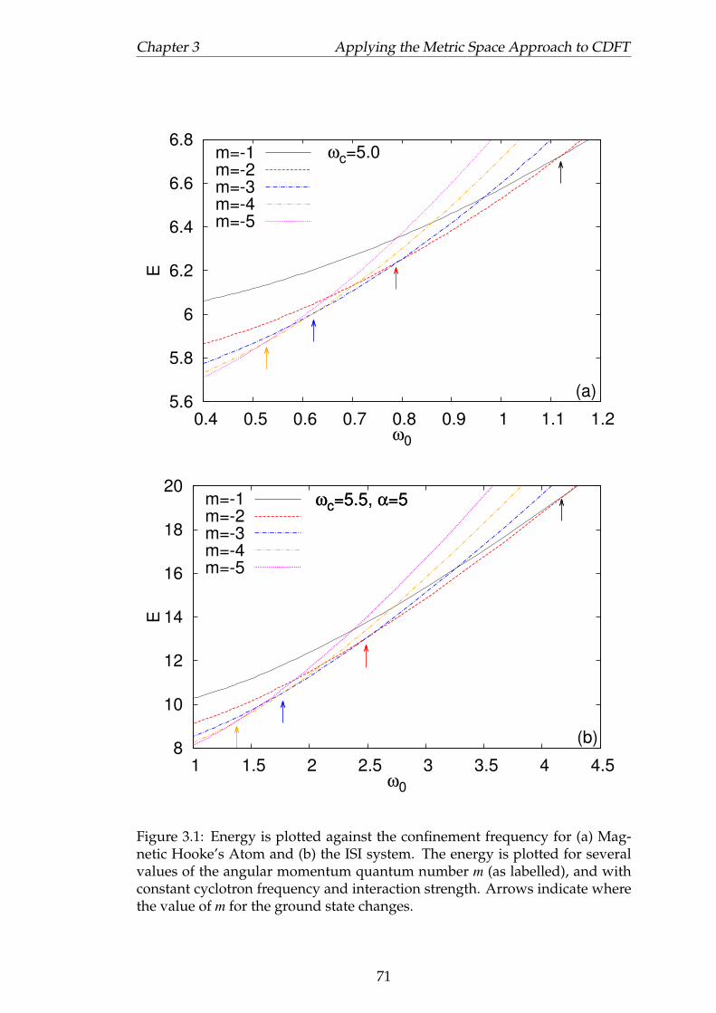
Chapter 3 Applying the Metric Space Approach to CDFT
5.6
5.8
6
6.2
6.4
6.6
6.8
0.4 0.5 0.6 0.7 0.8 0.9 1 1.1 1.2
E
ω0
ωc=5.0
(a)
m=-1m=-2m=-3m=-4m=-5
8
10
12
14
16
18
20
1 1.5 2 2.5 3 3.5 4 4.5
E
ω0
ωc=5.5, α=5
(b)
ωc=5.5, α=5m=-1m=-2m=-3m=-4m=-5
Figure 3.1: Energy is plotted against the confinement frequency for (a) Mag-netic Hooke’s Atom and (b) the ISI system. The energy is plotted for severalvalues of the angular momentum quantum number m (as labelled), and withconstant cyclotron frequency and interaction strength. Arrows indicate wherethe value of m for the ground state changes.
71
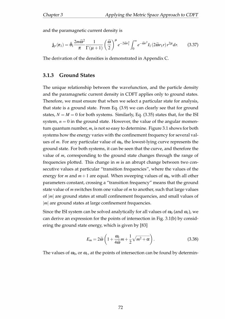
Chapter 3 Applying the Metric Space Approach to CDFT
and the paramagnetic current density is
jp (r1) = θ12mω2
π
1Γ(µ +1)
(ω
2
)µ
e−2ωr21
∫∞
0e−ωr2
I1 (2ωr1r)r2µdr. (3.37)
The derivation of the densities is demonstrated in Appendix C.
3.1.3 Ground States
The unique relationship between the wavefunction, and the particle densityand the paramagnetic current density in CDFT applies only to ground states.Therefore, we must ensure that when we select a particular state for analysis,that state is a ground state. From Eq. (3.9) we can clearly see that for groundstates, N = M = 0 for both systems. Similarly, Eq. (3.35) states that, for the ISIsystem, n = 0 in the ground state. However, the value of the angular momen-tum quantum number, m, is not so easy to determine. Figure 3.1 shows for bothsystems how the energy varies with the confinement frequency for several val-ues of m. For any particular value of ω0, the lowest-lying curve represents theground state. For both systems, it can be seen that the curve, and therefore thevalue of m, corresponding to the ground state changes through the range offrequencies plotted. This change in m is an abrupt change between two con-secutive values at particular “transition frequencies”, where the values of theenergy for m and m+1 are equal. When sweeping values of ω0, with all otherparameters constant, crossing a “transition frequency” means that the groundstate value of m switches from one value of m to another, such that large valuesof |m| are ground states at small confinement frequencies, and small values of|m| are ground states at large confinement frequencies.
Since the ISI system can be solved analytically for all values of ω0 (and ωc), wecan derive an expression for the points of intersection in Fig. 3.1(b) by consid-ering the ground state energy, which is given by [83]
Em = 2ω
(1+
ωc
4ωm+
12
√m2 +α
). (3.38)
The values of ω0, or ωc, at the points of intersection can be found by determin-
72

Chapter 3 Applying the Metric Space Approach to CDFT
ing the frequencies where Em = Em+1,
2ω
(1+
ωc
4ωm+
12
√m2 +α
)= 2ω
(1+
ωc
4ω(m+1)+
12
√(m+1)2 +α
),
ωc
2ωm+
√m2 +α =
ωc
2ω(m+1)+
√(m+1)2 +α,√
m2 +α =ωc
2ω+
√(m+1)2 +α,
ωc
2ω=
(√m2 +α−
√(m+1)2 +α
).
By writing
Ωm,α =√
m2 +α−√(m+1)2 +α, (3.39)
and using the definition of ω from Eq. (3.7), we have
ω2c
ω2c +4ω2
0= Ω
2m,α ,
ω2c = Ω
2m,αω
2c +Ω
2m,α4ω
20 ,
1 = Ω2m,α +4Ω
2m,α
ω20
ω2c.
This gives the following expression for the relationship between ω0 and ωc
when Em = Em+1, (ω0
ωc
)2
=1−Ω2
m,α
4Ω2m,α
. (3.40)
3.2 Varying the Confinement Potential
In Ref. [62], we concentrated on the sets of ground state wavefunctions, relatedparticle densities, and related paramagnetic current densities to study the rela-tionship between them at the core of CDFT. Since ground states are non-emptysubsets of all states, ground-state-related functions form metric spaces withthe metrics (2.18), (2.10), and (2.28). To produce families of ground states, foreach system we systematically vary the value of ω0 (while keeping all otherparameters constant), and for each value we calculate the ground state wave-function, particle density, and paramagnetic current density. A reference stateis determined by choosing a specific ω0 value, and the appropriate metric isthen used to calculate the distances between it and each member of the family.To ensure that we select ground states, varying ω0 may require varying thequantum number m [42, 83]. In Fig. 3.1, we see that as ω0 increases, we mustdecrease the value of |m| in order to remain in the ground state. As a result ofthis property, within each family of ground states, paramagnetic current den-
73

Chapter 3 Applying the Metric Space Approach to CDFT
0
0.4
0.8
1.2
1.6
2
0 0.8 1.6 2.4 3.2 4Dρ
ωc=5.5, α=5, mref=-10
(f)m=-11m=-12m=-13
m=-45m=-1
m=-2
m=-3
m=-4
m=-5
m=-6m=-7
m=-8m=-9
0
0.4
0.8
1.2
1.6
2
0 0.4 0.8 1.2 1.6 2 2.4Dψ
ωc=5.5, α=5, mref=-10
(d)m=-11m=-12
m=-13
m=-45m=-1
m=-2
m=-3
m=-4
m=-5
m=-6m=-7
m=-8m=-9
0
0.8
1.6
2.4
3.2
4
0 0.4 0.8 1.2 1.6 2 2.4Dψ
ωc=5.5, α=5, mref=-10
(b)m=-11m=-12
m=-13
m=-45m=-1
m=-2
m=-3
m=-4m=-5
m=-6m=-7
m=-8m=-9
0
0.4
0.8
1.2
1.6
0 0.4 0.8 1.2 1.6Dψ
ωc=5, mref=-5
(c)m=-6
m=-8
m=-10
m=-12
m=-4
m=-3
m=-2
m=-1
Dj p
⊥
2|m
1|+|m
2|
0
0.4
0.8
1.2
1.6
0 0.4 0.8 1.2 1.6 2 2.4Dρ
ωc=5, mref=-5
(e)m=-6
m=-8
m=-10
m=-12
m=-4
m=-3
m=-2
m=-1
Dj p
⊥
2|m
1|+|m
2|
0
0.4
0.8
1.2
1.6
2
0 0.4 0.8 1.2 1.6
Dρ
Dψ
ωc=5, mref=-5
(a)m=-6
m=-8
m=-10
m=-12Decreasing ω0
m=-4
m=-3
m=-2
m=-1Increasing ω0
Figure 3.2: Results for ground states. Left: Hooke’s atom (reference state ω0 =0.5,ωc = 5,mre f =−5). Right: ISI system (reference state ω0 = 0.62,ωc = 5.5,α =5,mre f =−10). Panels (a) and (b): Dρ vs Dψ ; (c) and (d): rescaled Djp⊥
vs Dψ ; (e)and (f): rescaled Djp⊥
vs Dρ . Frequencies smaller than the reference are labelledwith circles, larger with triangles.
74

Chapter 3 Applying the Metric Space Approach to CDFT
θmax
θmin
Δθ
Figure 3.3: With reference to the “onion-shell” geometry of our metric spaces,we define the maximum and minimum angles between paramagnetic currentdensities on each sphere and the reference. We also define the difference be-tween these angles as ∆θ .
sities will “jump” from one sphere of the onion-shell geometry to another (seeFig. 2.1, where the reference state is the “north pole” of its sphere). To obtainground states with non-zero paramagnetic current densities, we must use ω0
values corresponding to m < 0 [42, 83].
In Fig. 3.2, we plot the relationship between each pair of distances for the twosystems. The reference states have been chosen so that most of the availabledistance range can be explored both for the case of increasing and for the caseof decreasing values of ω0. When considering the relationship between groundstate wavefunctions and related particle densities, Figs. 3.2(a) and 3.2(b), ourresults confirm the findings in Ref. [58] (shown in Fig 1.1): a monotonic map-ping, linear for low to intermediate distances, where nearby wavefunctions aremapped onto nearby particle densities, and distant wavefunctions are mappedonto distant particle densities, and the curves for increasing and decreasing ω0
collapse onto each other. However closer inspection reveals a fundamentaldifference with Ref. [58], the presence of a “band structure.” By this we meanregions of allowed (“bands”) and forbidden (“gaps”) distances, whose widthsdepend on the value of |m|, at least for the systems considered here. This struc-ture is due to the changes in the value of the quantum number m, which resultin a substantial modification of the ground state wavefunction (and thereforeparticle density) and a subsequent large increase in the related distances.
When we focus on the plots of paramagnetic current densities’ against wave-functions’ distances, shown in Figs. 3.2(c) and 3.2(d), we find that the “bandstructure” dominates the behaviour. Here the change in |m| has an even stronger
75

Chapter 3 Applying the Metric Space Approach to CDFT
(b)(a)
Figure 3.4: Sketch of the “onion-shell” geometry of the metric space for param-agnetic current densities, where: (a)
∣∣mq∣∣> |mr|>
∣∣mre f∣∣ and (b)
∣∣mre f∣∣> |ms|>
|mt |. The reference state is at the north pole on the reference sphere. Thedark grey areas denote the regions where ground state currents are located(“bands”), with dashed lines indicating their widths. mq,r,s,t are arbitrary val-ues of the quantum number m, such that
∣∣mq∣∣> |mr|>
∣∣mre f∣∣> |ms|> |mt |.
effect, in that the gradient dDjp⊥/dDψ is noticeably discontinuous when mov-
ing from one sphere to the next in jp metric space. This discontinuity is morepronounced for the path |m| <
∣∣mre f∣∣ than for the path |m| >
∣∣mre f∣∣. Similarly
to Figs. 3.2(a) and 3.2(b), the mapping of Dψ onto Djp⊥maps vicinities onto
vicinities and remains monotonic, but for small and intermediate distances itis only piecewise linear. In contrast with Dρ vs Dψ , curves corresponding toincreasing and decreasing ω0 do not collapse onto each other.
Figures 3.2(e) and 3.2(f) show the mapping between particle and paramagneticcurrent density distances: this has characteristics similar to the one betweenDψ and Djp⊥
, but remains piecewise linear even at large distances.
We will now concentrate on the jp metric space to characterize the “band struc-ture” observed in Fig. 3.2. Within the metric space geometry, we consider thepolar angle θ between the reference jpre f and the paramagnetic current densityjp of angular momentum |m|. Using the law of cosines, θ is given by
cosθ =m2
re f +m2−D2jp⊥
(jpre f , jp)
2∣∣mre f
∣∣ |m| . (3.41)
We define the polar angles corresponding to the two extremes of a given bandas θmin and θmax, shown in Fig. 3.3. The width of each band is then ∆θ = θmax−θmin, and its position defined by θmin. We will now calculate the widths andpositions of the bands by sweeping the values of ω0 corresponding to ground
76

Chapter 3 Applying the Metric Space Approach to CDFT
0
0.1
0.2
0.3
0 2 4 6 8 10 12
θ/π
|m|
ωc=5.0, mref=-5
(a)
|mref|
θmaxθmin
∆θ
0
0.002
0.004
4 5 6 7
0
0.2
0.4
0.6
0.8
0 10 20 30 40
θ/π
|m|
ωc=5.5, α=5, mref=-10
(b)
|mref|
θmaxθmin
∆θ
0
0.002
0.004
9 10 11 12
Figure 3.5: Results of the angular displacement of ground state currents for(a) Hooke’s Atom and (b) the ISI system with the behaviour of ∆θ close to theorigin shown in the inset. Lines are a guide to the eye.
77

Chapter 3 Applying the Metric Space Approach to CDFT
states for each value of |m|.
For both systems under study, we find that as |m| increases from∣∣mre f
∣∣, bothθmax and θmin increase. This has the effect of the bands moving from the northpole to the south pole as we move away from the reference. Additionally, wefind that the bandwidth ∆θ decreases as |m| increases [sketched in Fig. 3.4(a)].As |m| decreases from
∣∣mre f∣∣, we again find that both θmax and θmin increase,
with the bands moving from the north pole to the south pole. However, thistime, as |m| decreases, ∆θ increases, meaning that the bands get wider as wemove away from the reference [sketched in Fig. 3.4(b)].
Quantitative results for Hooke’s Atom and the ISI system are shown in Fig. 3.5.The band on the surface of each sphere indicates where all ground state para-magnetic current densities lie within that sphere. In contrast with particle den-sities or wavefunctions, we find that, at least for the systems at hand, groundstate currents populate a well-defined, limited region of each sphere, whosesize and position display monotonic behaviour with respect to the quantumnumber m. This regular behaviour is not at all expected, as the CDFT-HK the-orem does not guarantee monotonicity in metric space, and not even that themapping of Dψ to Djp⊥
is single valued. In the CDFT-HK theorem ground statewavefunctions are uniquely determined only by particle and paramagneticcurrent densities together. In this sense we can look at the panels in Fig. 3.2as projections on the axis planes of a 3-dimensional DψDρDjp⊥
relation. Thecomplexity of the mapping due to the application of a magnetic field – thechanges in quantum number m – is fully captured by Djp⊥
only, as this is re-lated to the relevant conservation law. However the mapping from Dρ to Dψ
inherits the “band structure,” showing that the two mappings Djp⊥to Dψ and
Dρ to Dψ are not independent.
3.3 Varying the Electron Interaction
As well as the confining potential, the interaction between the electrons alsocontributes to the potential energy of our model systems. For the ISI system,the parameter α allows us to vary the strength of the electronic interaction,hence we can repeat the analysis of the CDFT-HK theorem in Sec. 3.2 for thecase of varying α . Additionally, |m| for the ground state increases as α in-creases, in contrast to the decrease in the ground state value of |m| shown inFig. 3.1 for ω0.
Figure 3.6 shows plots of each pair of distances. As was the case for Fig 3.2, allof the plots show a “band structure” corresponding to the value of the angu-
78

Chapter 3 Applying the Metric Space Approach to CDFT
0
1
2
3
4
0 0.5 1 1.5 2
Dρ
Dψ
ω0=1.0, ωc=5.5, mref=-15
(a)
m=-1
m=-12m=-13
m=-14
Decreasing α
m=-16m=-17
m=-18
m=-49Increasing α
0
0.5
1
1.5
2
0 0.5 1 1.5 2
Dj p
⊥
Dψ
ω0=1.0, ωc=5.5, mref=-15
(b)
m=-1
m=-12m=-13
m=-14
Decreasing α
m=-16m=-17
m=-18
m=-49Increasing α
0
0.5
1
1.5
2
0 1 2 3 4
Dj p
⊥
Dρ
ω0=1.0, ωc=5.5, mref=-15
(c)
m=-1
m=-12m=-13
m=-14
Decreasing α
m=-16m=-17
m=-18
m=-49Increasing α
Figure 3.6: Results for ground states for the ISI system when varying α (ref-erence state ω0 = 1.0,ωc = 5.5,α = 29.756,mre f = −15). The reference value ofα is taken halfway between the two “transition frequencies” related to mre f .Panel (a): Dρ vs Dψ ; (b): rescaled Djp⊥
vs Dψ ; (c): rescaled Djp⊥vs Dρ . Values of
α smaller than the reference are labeled with circles, larger with triangles.79

Chapter 3 Applying the Metric Space Approach to CDFT
lar momentum quantum number m, that consists of “bands” of distances foreach particular value of m separated by “gaps” of forbidden distances. Whenconsidering Dρ against Dψ [Fig. 3.6(a)], the path traced out by the curve is al-most identical to that in Fig. 3.2, and again depicts a monotonic relationshipbetween Dρ and Dψ which is almost linear for small to intermediate distancesand follows the same curve for the cases of increasing α and decreasing α .Figures 3.6(b) and 3.6(c) show that, as before, the “band structure” causes dis-continuities in the gradient when we introduce the paramagnetic current den-sity. However, in contrast to Fig. 3.2, the discontinuity in the gradient between“bands” is considerably less pronounced, and also as |m| decreases, the bandscover a smaller range of distances. Comparison of the results for both sys-tems in Fig. 3.2 and Fig. 3.6 suggests that as the reference value of |m| becomeslarger, the discontinuity in the gradient between bands is reduced. A conse-quence of the less pronounced discontinuity is that the curves for increasingand decreasing α are more similar than those for increasing and decreasing ω0.
Figure 3.7 shows the angular displacement of the bands on each of their metricspace spheres for the paramagnetic current density. As for the case of varyingω0, we observe that the bands move from the north pole to the south pole as wedepart from mre f , and that the bands get narrower as |m| increases. However,we note that the width of the bands, particularly for small values of |m|, areconsiderably smaller compared to those in Fig. 3.5. Consequently, the band-width is plotted in Fig. 3.7(b), in which we observe that the width of the bandfor mre f is considerably smaller than the bands corresponding to all nearbyvalues of m. We suggest that this is an artifact of the arbitrary choice of our ref-erence, especially given that the shape of the reference band is different fromall of the others, as depicted in Fig. 3.4. Comparing with the case of varyingω0, the insets of Fig. 3.5 show a similar decrease in the bandwidth for the ISIsystem, but not for Hooke’s Atom (albeit we do observe a discontinuity in thegradient of the overall decrease in ∆θ ).
In conclusion, we find that the metric space approach to quantum mechanicsoffers considerable insight into the mapping at the core of CDFT. The mappingbetween the fundamental quantities in CDFT inherits the features observedfor standard DFT. However, varying the potential energy through either theconfinement potential or the strength of the electronic interaction introduces a“band structure” into the ground state metric spaces for wavefunctions, parti-cle densities and paramagnetic current densities; a feature that is entirely ab-sent when a magnetic field is not present. The origin of the “band structures”is changes in the value of the quantum number for the angular momentum, m,and the value of |m| is shown to control the shape of the “bands”.
80

Chapter 3 Applying the Metric Space Approach to CDFT
0
0.2
0.4
0.6
0.8
0 10 20 30 40 50
θ/π
|m|
ω0=1, ωc=5.5, mref=-15
(a)
|mref|
θmaxθmin
∆θ
0
0.0025
0.005
0.0075
0.01
0.0125
0 10 20 30 40 50
θ/π
|m|
ω0=1, ωc=5.5, mref=-15
(b)
|mref|
∆θ
Figure 3.7: Results of the angular displacement of ground state currents whenvarying α for the ISI system. Panel (a) shows θmax, θmin and ∆θ , and we focuson ∆θ in panel (b). Lines are a guide to the eye.
81
Chapter 4
Exploring the Effects of VaryingMagnetic Fields With the MetricSpace Approach
In Chapter 3, we have shown the effect of changes in the scalar and electronicinteraction potentials on the wavefunction, particle density and paramagneticcurrent density, and their unique relationship for ground states, as defined inCDFT. However, a quantity far more amenable to varying experimentally isthe strength of the magnetic field itself. Systems immersed in magnetic fieldsare subject to a vector potential, A(r), which represents the magnetic field inthe Hamiltonian (1.5). Hence, by exploring changes in this vector potential,we can use the metric space approach to quantum mechanics to study systemssubject to a magnetic field as the field changes.
Systems immersed in magnetic fields are a fundamental research topic, for ex-ample, atoms immersed in strong fields [84, 85], and phenomena such as nu-clear magnetic resonance [86] and the quantum hall effect [87]; and are also anintegral part of emerging quantum technologies such as quantum computationwhich utilise quantum systems controlled or otherwise affected by magneticfields. For example the inhomogeneous magnetic field generated by the nu-clei’s spins decreases quantum coherence of electron spin qubits in III-V quan-tum dots [88], while full polarisation of the spin bath through an applied mag-netic field suppresses electron-spin decoherence in nitrogen-vacancy centresand nitrogen impurities in diamond [89]. Understanding systems immersedin a magnetic field at a quantum level is therefore both of fundamental andtechnological importance.
Varying the strength of the magnetic field for ground state systems will allowus to enhance the insights into the fundamental relationship between the ba-
82
Chapter 4 Exploring the Effects of Varying Magnetic Fields
sic variables of CDFT provided by the results in Chapter 3. In particular, inthe presence of a magnetic field, the metric spaces for ground state wavefunc-tions, particle densities and paramagnetic current densities are characterisedby a “band structure” [62]. In paramagnetic current density metric space,when considering variations in the scalar potential [62], the “band structure”is formed by spherical segments of allowed and forbidden distances on the con-centric spheres, at least for the systems analysed. The specific arc length ofthese segments varies depending on the radius |m| of the sphere. The “bandstructure” of allowed and forbidden distances also presents itself in the metricspaces for wavefunctions and particle densities, but only on a single sphere inthese cases. We will investigate how this “band structure” responds to changesin the magnetic field.
One of the key strengths of the metric space approach to quantum mechanicsis that it can easily be applied to excited states as well as ground states, whichmakes the approach a widely applicable tool for the study of many-body sys-tems. We will then study the relationship between the wavefunction, particledensity and paramagnetic current density for excited states when varying themagnetic field, and compare and contrast the results with those for groundstates.
The results in this chapter were published in Ref. [63].
4.1 Ground States
4.1.1 Ground States of Model Systems
We again focus on the model systems employed in Chapter 3: the magneticHooke’s Atom and the Inverse Square Interaction (ISI) system [42, 75, 83]. Wevary the strength of the magnetic field via the cyclotron frequency, ωc. Onceagain, we must ensure that the value of the angular momentum quantum num-ber m is such that we are in the ground state for all values of ωc.
Figure 4.1 shows how the energy varies with the cyclotron frequency for sev-eral values of m, with the lowest-lying curve representing the ground state, asin Fig. 3.1. As was the case for the confinement frequency, Fig. 4.1 shows thatthe ground state value of m changes as we sweep through the values of ωc,with abrupt changes in the ground state value of m at “transition frequencies”.However, there is one significant difference which is that when varying ωc, thevalue of |m| for the ground state increases as ωc increases. This difference indi-cates that the relationship between the basic variables in CDFT may differ as
83

Chapter 4 Exploring the Effects of Varying Magnetic Fields
4
6
8
10
0 2 4 6 8 10
E (
a.u
.)
ωc (a.u.)
ω0=1.0
(a)
m=0m=-1m=-2m=-3m=-4
4
6
8
10
0 1 2 3 4 5 6
E (
a.u
.)
ωc (a.u.)
ω0=1.0, α=5.0
(b)
m=0m=-1m=-2m=-3m=-4
Figure 4.1: Energy is plotted against the cyclotron frequency for several valuesof m for (a) Magnetic Hooke’s Atom and (b) the ISI system. The confinementfrequency and interaction strength are held constant. Arrows indicate wherethe value of m for the ground state changes.
84

Chapter 4 Exploring the Effects of Varying Magnetic Fields
we vary the vector potential compared to varying the scalar potential.
As in Chapter 3, we generate families of states, this time by varying the mag-netic field via the cyclotron frequency ωc, whilst holding the confinement fre-quency, ω0, and all other parameters in the Hamiltonian constant. Within eachfamily, one value of ωc (and hence m) is selected as a reference (ωcre f ,mre f re-spectively), with the appropriate metrics used to find the distance between thephysical functions at the reference and all of the others in the family.
4.1.2 Band Structure of Metric Spaces
We will start by comparing the distances between wavefunctions, their relatedparticle densities and their related paramagnetic current densities. Figure 4.2shows plots of the relationships between the various distances considered,with each point referring to a particular value of ωc. Let us consider first theplots of particle density distance against wavefunction distance [Figs. 4.2(a)- 4.2(d)]. As observed in Chapter 3, metric space regions corresponding toground states present a “band structure”, where points associated to the samevalue of |m| are grouped into distinct segments, i.e., bands. However, in con-trast to the band structure observed in Chapter 3 [sketched in Fig. 4.3(a)], whenvarying the vector potential we obtain a series of “overlapping bands”, wherethe minimum wavefunction and minimum particle density distances for onevalue of |m| are smaller than the maximum distances for the previous valueof |m|. This implies that there is now an overlap between the projections ofthe bands on the metric space sphere representing the densities, as sketchedin Fig. 4.3(b) (similarly for the projection on the sphere representing the wave-functions). Though overlapping, this band structure still results in disconti-nuities in the relationship between Dρ and Dψ when the value of m changes.Unlike when varying ω0 [62], by varying the magnetic field we do not observeany forbidden distances, so we cannot identify forbidden regions for groundstates by considering the density and wavefunction metric spaces alone. Inthe range of distances explored here, nearby wavefunctions are mapped ontonearby particle densities and distant wavefunctions are mapped onto distantparticle densities. However, in contrast to Chapter 3, the mapping is onlypiecewise linear; when acting on the vector potential, as ωc is swept througheach “transition” frequency, ground states and their densities abruptly revertto be closer to the reference state, while a (almost) linear mapping is main-tained within two consecutive “transition” frequencies. Also, in contrast withthe results in Chapter 3, the two families of ground states corresponding to|m| <
∣∣mre f∣∣ and |m| >
∣∣mre f∣∣ describe distinct paths in metric space [e.g., com-
85

Chapter 4 Exploring the Effects of Varying Magnetic Fields
0
0.4
0.8
1.2
1.6
0 0.4 0.8 1.2
Dρ
Dψ
ω0=0.5, mref=-5
(a)
m=-1
m=-2
m=-3
m=-4
Decreasing ωc
0
0.4
0.8
1.2
0 0.2 0.4 0.6 0.8 1 1.2
Dρ
Dψ
ω0=0.5, mref=-5
(b)m=-6
m=-7m=-8
m=-20Increasing ωc
0
0.4
0.8
1.2
0 0.2 0.4 0.6 0.8 1 1.2
Dρ
Dψ
ω0=0.6, α=5, mref=-10
(c)
m=-1m=-2
m=-3m=-4
m=-5m=-6
m=-7m=-8
m=-9
0
0.4
0.8
1.2
0 0.4 0.8 1.2
Dρ
Dψ
ω0=0.6, α=5, mref=-10
(d)m=-11m=-12
m=-13
m=-50
0
0.4
0.8
1.2
1.6
0 0.4 0.8 1.2Dψ
ω0=0.5, mref=-5
(e)
m=-1
m=-2
m=-3
m=-4
Dj p
⊥
2|m
1|+|
m2|
0
0.4
0.8
1.2
0 0.2 0.4 0.6 0.8 1 1.2Dψ
ω0=0.5, mref=-5
(f)m=-6
m=-7m=-8
m=-20
Dj p
⊥
2|m
1|+|
m2|
0
0.4
0.8
1.2
1.6
0 0.4 0.8 1.2 1.6Dρ
ω0=0.5, mref=-5
(i)
m=-1
m=-2
m=-3
m=-4
Dj p
⊥
2|m
1|+|
m2|
0
0.4
0.8
1.2
0 0.4 0.8 1.2Dρ
ω0=0.5, mref=-5
(j)m=-6
m=-7m=-8
m=-20
Dj p
⊥
2|m
1|+|
m2|
0
0.4
0.8
1.2
1.6
0 0.2 0.4 0.6 0.8 1 1.2Dψ
ω0=0.6, α=5, mref=-10
(g)
m=-1
m=-2
m=-3m=-4
m=-5m=-6
m=-7m=-8
m=-9
Dj p
⊥
2|m
1|+|
m2|
0
0.4
0.8
1.2
1.6
0 0.4 0.8 1.2Dρ
ω0=0.6, α=5, mref=-10
(k)
m=-1
m=-2
m=-3m=-4
m=-5m=-6
m=-7m=-8
m=-9
Dj p
⊥
2|m
1|+|
m2|
0
0.4
0.8
1.2
0 0.4 0.8 1.2Dψ
ω0=0.6, α=5, mref=-10
(h)m=-11m=-12
m=-13
m=-50
Dj p
⊥
2|m
1|+|
m2|
0
0.4
0.8
1.2
0 0.4 0.8 1.2 1.6Dρ
ω0=0.6, α=5, mref=-10
(l)m=-11m=-12
m=-13
m=-50
Dj p
⊥
2|m
1|+|
m2|
Figure 4.2: Plots of distances for Hooke’s Atom with reference state ω0 =0.5,ωc = 5.238,mre f = −5 (top two rows) and for the ISI system with refer-ence state ω0 = 0.6,ωc = 5.36,α = 5,mre f = −10 (bottom two rows). (a) - (d)show particle density distance against wavefunction distance, (e) - (h) showparamagnetic current density distance against wavefunction distance and (i)- (l) show paramagnetic current density distance against particle density dis-tance. The reference frequency is taken halfway between the two “transitionfrequencies” related to mre f .
pare Figs. 4.2(a) and 4.2(b)], with the size of the bands greater for |m| <∣∣mre f
∣∣compared to |m| >
∣∣mre f∣∣. For all of these reasons the CDFT-HK mapping be-
tween wavefunctions and related densities acquires added complexity whenvarying the vector potential compared to varying the scalar potential [com-pare Figs. 3.2(a) and 3.2(b) with Figs. 4.2(a) - 4.2(d)].
In Figs. 4.2(e) - 4.2(h) we consider paramagnetic current density distance againstwavefunction distance. Here we find once more an overlapping band structurefor wavefunction distances, however a band structure with regions of allowed(“bands”) and forbidden (“gaps”) distances is observed for paramagnetic cur-rent density distances. In contrast with the one sketched in Fig. 4.3(a), in thiscase each band resides on a different sphere according to the value of |m| (the
86

Chapter 4 Exploring the Effects of Varying Magnetic Fields
Figure 4.3: Sketches of “band structures” consisting of (a) “bands” and “gaps”and (b) “overlapping bands” in particle density metric space for three consec-utive bands, where a different patterning corresponds to a different value ofm. The reference state is at the north pole.
radius of the sphere). For both wavefunction and paramagnetic current den-sity distances, there are discontinuities between the bands. As for Figs. 4.2(a) -4.2(d), the curves for increasing and decreasing ωc (and hence |m|) do not over-lap, with larger bands for small values of |m|. Finally Figs. 4.2(i) - 4.2(l) presentthe plots of paramagnetic current density distance against particle density dis-tance. These exhibit similar behaviour to Figs. 4.2(e) - 4.2(h).
The overlapping band structures observed in Fig. 4.2 demonstrate that map-pings between some of the distances considered here are multivalued. Thismultivalued mapping does not represent a contradiction of the CDFT-HK the-orem as it is entirely possible to have distinct functions at the same distanceaway from a reference. In particular, in terms of the “onion-shell” geometry,all states situated at the same polar angle and on the same sphere will have thesame distance from the reference state.
In Fig. 4.4 the wavefunction and paramagnetic current density distances areplotted against ωc for both systems, enabling the band structures for individ-ual functions to be analysed. We firstly note that, as observed in Fig. 4.2, thereis a decrease in the wavefunction distance at transitions [Figs. 4.4(a) and 4.4(b)],but an increase in the paramagnetic current density distance [Figs. 4.4(c) and4.4(d)]. These features give rise to “overlapping bands” and “bands and gaps”band structures respectively. The other major feature is that, when varyingωc, there is non-monotonic behaviour within bands corresponding to valuesof m close to mre f (see insets). For both wavefunctions and paramagnetic cur-
87

Chapter 4 Exploring the Effects of Varying Magnetic Fields
0
0.4
0.8
1.2
0 5 10 15 20 25
Dψ
ωc (a.u.)
ω0=0.5, mref=-5
(a)
m=-1
m=-2
m=-3
m=-4m=-6
m=-7
m=-8.
..
m=-20
0
0.2
0.4
0.6
4 6 8 0
0.4
0.8
1.2
1.6
0 5 10 15 20 25
Dj p
⊥
ωc (a.u.)
ω0=0.5, mref=-5
(c)
m=-1
m=-2
m=-3
m=-4m=-6
m=-7
m=-8.
..
m=-20
0
0.2
0.4
0.6
4 6 8
0
0.4
0.8
1.2
0 5 10 15 20 25 30
Dψ
ωc (a.u.)
ω0=0.6, α=5, mref=-10
(b)m=-11m=-12m=-13
...
m=-50m=-1
m=-2
m=-3
m=-4
m=-5
m=-6
m=-7m=-8m=-9 0
0.1
0.2
0.3
4 5 6 7 0
0.4
0.8
1.2
1.6
0 5 10 15 20 25 30
Dj p
⊥
ωc (a.u.)
ω0=0.6, α=5, mref=-10
(d)m=-11m=-12m=-13
...
m=-50
m=-1
m=-2
m=-3
m=-4
m=-5
m=-6
m=-7
m=-8m=-9 0
0.1
0.2
0.3
0.4
4 5 6 7
Figure 4.4: For Hooke’s Atom (top) and the ISI system (bottom), wavefunctiondistance [(a) and (b)] and paramagnetic current density distance [(c) and (d)]are plotted against ωc. The behaviour around the reference frequency is shownin each inset. The reference states are ω0 = 0.5,ωcre f = 5.238,mre f = −5 for theMagnetic Hooke’s Atom and ω0 = 0.6,ωcre f = 5.36,α = 5,mre f =−10 for the ISIsystem.
rent densities, we observe that immediately after each transition frequency, thedistances initially decrease to a minimum for that particular band, before in-creasing to the maximum for the band. This occurs at the transition frequencyto the next band. This behaviour is more pronounced for wavefunctions thanfor paramagnetic current densities. As stated, the non-monotonicity is not incontradiction with the Hohenberg-Kohn theorem of CDFT, but shows a richerbehaviour with respect to what was observed in Chapter 3 when varying thescalar potential.
We point out that the band structure in metric space for paramagnetic currentdensity is fundamentally different from the ones for particle density and wave-function, as the first develops on different spheres, one band for each sphere,while the latter are within a single sphere where they may display “distinct” or“overlapping” bands, see Fig. 4.3. All these band structures originate from theconservation law characterising the paramagnetic current density, and the fea-tures of the metric spaces for wavefunctions and particle densities are a directconsequence of the mapping of jp (r) onto ψ (r) and onto ρ (r). In this sensethe band structure features of the metric spaces for wavefunctions and particle
88

Chapter 4 Exploring the Effects of Varying Magnetic Fields
0
0.5
1
1.5
2
0 0.2 0.4 0.6 0.8 1 1.2
(Dj p
⊥/D
ρ)2
|m1|
+|m
2|
Dψ
ω0=0.5, mref=-5
(a)
Decreasing ωcIncreasing ωc
0
0.4
0.8
1.2
1.6
0 0.2 0.4 0.6 0.8 1 1.2Dψ
ω0=0.6, α=5, mref=-10
(b)
Decreasing ωcIncreasing ωc
(Dj p
⊥/D
ρ)2
|m1|
+|m
2|
m=mref
m=mref
Figure 4.5: Plots of the ratio of paramagnetic current density distance to par-ticle density distance against wavefunction distance for (a) Magnetic Hooke’sAtom with reference state ω0 = 0.5,ωcre f = 5.238,mre f =−5, and (b) the ISI sys-tem with reference state ω0 = 0.6,ωcre f = 5.36,α = 5,mre f =−10.
89

Chapter 4 Exploring the Effects of Varying Magnetic Fields
densities could be seen merely as the “projections” of the band structure char-acterising the paramagnetic current density, that result from these mappings.
Finally, we wish to concentrate on the implications of our findings for CDFT.CDFT requires that both ρ (r) and jp (r) are taken together to ensure a one-to-one mapping to the wavefunction. The metric analysis allows us to provideevidence for an important aspect of this mapping, that is to understand therelative contributions of ρ (r) and jp (r) when mapping to the wavefunction,which may provide insight as to when the inclusion of jp (r) in the mappingbecomes really crucial for the one-to-one correspondence to hold.
We present in Fig. 4.5 the ratio Djp⊥/Dρ against Dψ for both the Magnetic
Hooke’s atom and the ISI system. From the data it is immediately clear that,in metric space, to a good level of approximation, Djp⊥
= const ×Dρ as longas m = mre f . This constant is the same for ωc > ωcre f and ωc < ωcre f . Thesefindings suggest that, at least for the systems at hand, as long as we remainon the same sphere in the paramagnetic current density metric space, jp (r) andρ (r) carry very similar information and the role of jp (r) in the core mappingof CDFT is secondary. The situation becomes very different for ground stateswith m 6= mre f . In this case the ratio Djp⊥
/Dρ is far from constant and Fig. 4.5clearly shows that the information contents of jp (r) and ρ (r) are both neces-sary to define the state.
To support these results, we will analyse in the next section the behaviour ofstates where m is kept equal to mre f at all values of ωc.
4.2 Excited States
Although an understanding of the ground state is important, for studying sys-tems subject to magnetic fields it is often necessary to go beyond ground states,for example, when studying rapidly varying fields or spintronic devices thatoperate with excited states. With the metrics at hand, we investigate for thefirst time excited states, and consider distances between families of states cor-responding to fixed values of m.1 For each value of m, we will construct afamily of states by varying ωc (with ω0 and α kept constant), and calculatingthe corresponding wavefunctions, particle densities and paramagnetic currentdensities. As for ground states, we choose m < 0. With respect to Fig. 4.1,this corresponds to following individual energy curves smoothly, i.e., with-out switching to a different curve at crossings, as done for the ground statecase. Each family of states will then lie on a particular sphere in the paramag-
1The centre of mass quantum number, M, is held constant at zero throughout this analysis.
90

Chapter 4 Exploring the Effects of Varying Magnetic Fields
0
1
2
3
4
0 0.5 1 1.5 2
Dρ
Dψ
ω0=0.1
(a)
m=-1m=-1m=-2m=-2m=-3m=-3
m=-8m=-8m=-9m=-9
m=-10m=-10
0
1
2
3
4
0 0.5 1 1.5 2
Dρ
Dψ
ω0=0.1, α=5
(b)
0
0.5
1
1.5
2
0 0.5 1 1.5 2Dψ
ω0=0.1
(c)
2|m
1|+|
m2|
Dj p
⊥
0
0.5
1
1.5
2
0 0.5 1 1.5 2Dψ
ω0=0.1, α=5
(d)
2|m
1|+|
m2|
Dj p
⊥
0
0.5
1
1.5
2
0 1 2 3 4Dρ
ω0=0.1, α=5
(f)
2|m
1|+|
m2|
Dj p
⊥
0
0.5
1
1.5
2
0 1 2 3 4Dρ
ω0=0.1
(e)
2|m
1|+|
m2|
Dj p
⊥
Figure 4.6: Plots of: (a) and (b) particle density distance against wavefunctiondistance, (c) and (d) paramagnetic current density distance against wavefunc-tion distance, (e) and (f) paramagnetic current density distance against particledensity distance for m =−1,−2,−3,−8,−9,−10. The reference states, for eachvalue of m, are: For Hooke’s Atom (left) ω0 = 0.1,ωcre f = 30.0, and for the ISIsystem (right), ω0 = 0.1,ωcre f = 5.0,α = 5. Closed symbols represent decreasingωc and open symbols represent increasing ωc.
91

Chapter 4 Exploring the Effects of Varying Magnetic Fields
0
5
10
15
20
0 0.5 1 1.5 2
Dj p
⊥
Dψ
ω0=0.1, α=5m=-1m=-1m=-2m=-2m=-3m=-3m=-8m=-8m=-9m=-9
m=-10m=-10
Figure 4.7: Plot of paramagnetic current density distance against wavefunctiondistance for m = −1,−2,−3,−8,−9,−10 for the ISI system. We take the statewith ω0 = 0.1,ωcre f = 5.0,α = 5 as a reference for each value of m and considerdistances across the surface of each individual sphere.
netic current density metric space. As the states considered are not necessar-ily ground states, there is no one-to-one mapping between the wavefunctionand particle and paramagnetic current densities, but, these being fundamentalquantities that characterise the system, we will still explore their relationships.Additionally, the study of these quantities allows us to corroborate the findingsrelated to Fig. 4.5.
Fig. 4.6 shows the relationship between each pair of distances for six differentvalues of m. For each pair of distances discussed, we find a monotonic rela-tionship that is linear in the low to intermediate distance regime, before one ofthe two functions rises more sharply to its maximum (see also Fig. 4.7). Themapping between the each of the three physical functions considered is suchthat nearby functions are mapped onto nearby functions and distant functionsare mapped onto distant functions for each function set. Crucially, as opposedto ground states, the distances do not form any kind of metric space “bandstructure” – confirming that the origin of band structures is changes in m.
Looking at wavefunction distances against particle density distances, Figs. 4.6(a)and 4.6(b), and contrasting with Figs. 4.2(a)-4.2(d), we observe that the curves
92

Chapter 4 Exploring the Effects of Varying Magnetic Fields
for increasing and decreasing ωc and all values of |m| collapse onto one an-other. This hints to a universal behaviour of the mapping between particledensity and wavefunction when all the physical quantities describing the sys-tem remain on the same sphere in the related metric space whilst a physicalparameter is smoothly changed.
When considering paramagnetic current density distance against wavefunc-tion distance in Figs. 4.6(c) and 4.6(d), although the curves for increasing anddecreasing ωc collapse onto one another, the curves for different values of m aredistinct, particularly when |m| is low. For lower values of |m| the linear regionextends across a larger range of distances. There is also a relatively small in-crease in the gradient at greater distances for low |m|. The curves in Figs. 4.6(c)and 4.6(d) all start and end at the same points. With the rescaling for Djp⊥
usedin Fig. 4.6, the curves tend to a limiting curve with increasing value of |m|. InFig. 4.7, we show the relationship between wavefunction distance and para-magnetic current density distance for the ISI system without rescaling Djp⊥
.Here, the curves for each value of |m| intersect only at the origin, and each hasa unique maximum of 2 |m| for the paramagnetic current density distance. Weobserve that the gradient of the initial linear region increases with |m|. Fig-ure 4.8 shows, for both systems, that the gradient in this region increases lin-early with |m|, Djp⊥
≈ k |m|Dψ , with k≈ 0.69 for Hooke’s Atom and k≈ 0.68 forthe ISI system, and is approximately equal for both decreasing and increasingωc. These results imply that when rescaled as in Fig. 4.6, the initial slope of thecurves will always be below 45, a result also observed in Ref. [58] for the casein which different spheres in the wavefunction metric space geometry wereconsidered.
When considering paramagnetic current density distance against particle den-sity distance [Figs. 4.6(e) and 4.6(f)] we see that, as for Djp⊥
vs Dψ , with therescaling of Fig. 4.6 there are distinct curves for each value of m which con-verge onto a single curve as |m| increases. As opposed to Djp⊥
vs Dψ , the extentof the linear behaviour of these curves is increasing as |m| increases.
The behaviour of the curves observed in Fig. 4.6 reflects the “onion-shell”geometry of the metric spaces. For wavefunctions and particle densities thesphere radius is associated to the number of particles in the system, which isfixed for the systems considered. Thus, regardless of the value of |m|, wave-functions and particle densities always lie on the same sphere in their respec-tive metric spaces. The fact that the related curves still superimpose for differ-ent values of |m| seems to imply that the value of |m| has no significant effect onthe curves that represent the relative change of ψ and ρ for changing parame-ters. In paramagnetic current density metric space, the sphere radius is related
93

Chapter 4 Exploring the Effects of Varying Magnetic Fields
0
1
2
3
4
5
6
7
1 2 3 4 5 6 7 8 9 10
Dj p
⊥
/Dψ
|m|
ω0=0.1
(a)
ωc=12.5ωc=17.5
0
1
2
3
4
5
6
7
1 2 3 4 5 6 7 8 9 10
Dj p
⊥
/Dψ
|m|
ω0=0.1, α=5.0
(b)
ωc=4.5ωc=6.0
Figure 4.8: Plot of the ratio of paramagnetic current density distance to wave-function distance against |m| for (a) Magnetic Hooke’s Atom, with referenceω0 = 0.1,ωcre f = 30.0, and (b) the ISI system, with reference ω0 = 0.1,ωcre f =5.0,α = 5. The gradient is taken at the frequencies corresponding to the clos-est points to ωcre f for both decreasing and increasing ωc in Fig. 4.7, which forHooke’s Atom are ωc = 12.5 for decreasing frequencies and ωc = 17.5 for in-creasing frequencies, and for the ISI system are ωc = 4.5 for decreasing fre-quencies and ωc = 6.0 for increasing frequencies.
94

Chapter 4 Exploring the Effects of Varying Magnetic Fields
to |m|, so paramagnetic current densities are on the surface of different sphereseach time we consider a different value of |m|. As a result we see that the shapeeach of the curves is affected and they do not collapse onto each other. A sim-ilar “universal” behaviour within each sphere and, by contrast, the breakingof this universality when different spheres were considered was also observedin Ref. [58], where different values of N, and hence different spheres, for bothwavefunctions and particle densities were considered. This seems to suggestthat different behaviour for the mappings should be expected when curves ondifferent spheres in the metric spaces are involved.
Finally Fig. 4.9 combines all distances for each system in a single plot. Im-portantly this figure shows that for small to medium wavefunction distancesDjp⊥
/Dρ ∼ const, where the constant depends on |m|, so that this ratio is in-dependent over variations of the wavefunction for relatively close wavefunc-tions. In this respect, for relatively close wavefunctions this suggests that themappings between paramagnetic current densities and wavefunctions, andbetween particle densities and wavefunctions, are very similar, as long as thefamily of states follows the evolution of the same energy curve as driven bythe varying parameter (see Fig. 4.1).
In conclusion we have shown that varying the magnetic field has a profoundeffect on the “band structure” in ground state metric spaces, illustrating theimportant role played by the vector potential in such systems, and providingadditional insight into the CDFT-HK theorem. Changes in the magnetic fieldgenerate a “band structure” that consists of overlapping bands for the wave-function and particle density, whilst the gaps of forbidden distances observedwhen varying quantities related to the scalar potential in Chapter 3 were notobserved for the wavefunction or particle density. Combining the metrics forthe particle and paramagnetic current densities and comparing with wave-function distances, we find that the nature of the ratio of the paramagneticcurrent density distance to the particle density distance has a strong depen-dence on whether or not the values of m are the same for the two functionsconsidered to calculate each distance. When m = mre f , the ratio is a constantdepending on m, but when m 6= mre f , the value of the ratio fluctuates consider-ably. We also gain additional insight into the geometry of our metric spaces byexploring excited states, where we observe that the value of m studied affectsthe relationships involving the metric for the paramagnetic current density, thegeometry of which is characterised by the angular momentum quantum num-ber. When considering the ratios of paramagnetic current density to particledensity distances, the constant relationship found for ground states is shownto persist up to fairly large values of the wavefunction distance.
95
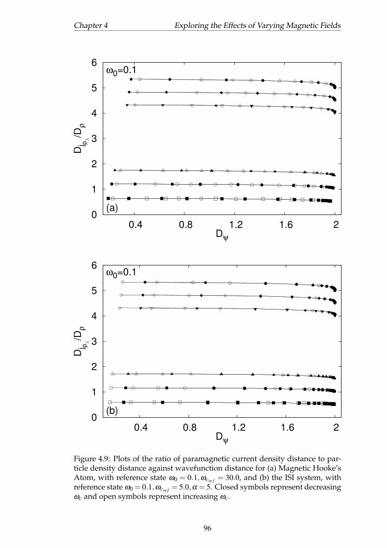
Chapter 4 Exploring the Effects of Varying Magnetic Fields
0
1
2
3
4
5
6
0.4 0.8 1.2 1.6 2
Dj p
⊥
/Dρ
Dψ
ω0=0.1
(a)
0
1
2
3
4
5
6
0.4 0.8 1.2 1.6 2
Dj p
⊥
/Dρ
Dψ
ω0=0.1
(b)
Figure 4.9: Plots of the ratio of paramagnetic current density distance to par-ticle density distance against wavefunction distance for (a) Magnetic Hooke’sAtom, with reference state ω0 = 0.1,ωcre f = 30.0, and (b) the ISI system, withreference state ω0 = 0.1,ωcre f = 5.0,α = 5. Closed symbols represent decreasingωc and open symbols represent increasing ωc.
96

Chapter 5
Comparing Many-Body andKohn-Sham Systems Using theMetric Space Approach
The vast majority of practical implementations of DFT make use of the Kohn-Sham scheme, where the system of interacting electrons confined within a par-ticular potential is replaced with an auxiliary system of non-interacting elec-trons confined by a different potential. The particle density of this auxiliarysystem is identical to that generated by the original many-body interactingsystem. The principle reason for the success of the Kohn-Sham scheme is thatthe majority of the Kohn-Sham potential is known, and the unknown part ofthe Kohn-Sham potential, the exchange-correlation potential, Vxc, can be effec-tively approximated. Indeed, even relatively crude approximations to Vxc canyield good results [24].
So far, the metric space approach to quantum mechanics has been used toexplore the relationships between wavefunctions and densities for DFT andCDFT. In order to further our understanding of the fundamentals of DFT wewill now investigate the Kohn-Sham scheme with the metric space approach,which has already been attempted [90]. In this chapter we will apply ourmetrics to the wavefunctions and potentials used to describe systems in themany-body picture, alongside the wavefunctions and potentials used in theKohn-Sham description. We will compare the distances between many-bodyand Kohn-Sham quantities as we vary a particular parameter for model quan-tum systems. We will also use our metrics to determine distances betweenthe many-body and Kohn-Sham quantities that describe the same system, pro-viding a quantitative analysis of how the effective quantities employed in theKohn-Sham picture differ from those of the many-body picture.
97

Chapter 5 Comparing MB and KS Systems Using the Metric Space Approach
In addition, our metric for potentials allows us to expand on the analysis ofthe HK theorem in Ref. [58], by considering the unique relationship betweenpotentials and wavefunctions and, consequently, potentials and densities, de-fined in standard DFT. We will also compare and contrast the informationgiven by each of the three metrics in order to assess the relative merits of eachof our three metrics for quantitative comparisons of many-body systems.
The results in this chapter are ongoing research [64].
5.1 Model Systems
In this chapter, we require model systems from which we can obtain both themany-body and Kohn-Sham quantities with high accuracy. Since it is possibleto reverse engineer the Kohn-Sham equations exactly for systems of two elec-trons [91–93], we will study two-electron model systems: Hooke’s Atom andHelium-like atoms.
5.1.1 Hooke’s Atom
The Hamiltonian for the three-dimensional Hooke’s Atom is [73]
H =12(p2
1 +ω20 r2
1 +p22 +ω
20 r2
2)+
1|r1− r2|
. (5.1)
We solve this system using the method in Ref. [73], which is exactly analagousto the method used for solving the Magnetic Hooke’s Atom in Sec. 3.1.1 [75].
In centre of mass and relative motion coordinates, the Hamiltonian is
H =14
p2R +ω
20 R2 +p2
r +14
ω20 r2 +
1r. (5.2)
The Hamiltonian for the centre of mass is simply that of a one-particle har-monic oscillator, hence the solution is given by [1, 10]
ξ (R)=Hn1
(√2ω0Rsinθ cosφ
)Hn2
(√2ω0Rsinθ sinφ
)Hn3
(√2ω0Rcosθ
)e−ω0R2
,
(5.3)and the normalised, ground-state wavefunction is
ξ0 (R) =
(2ω0
π
) 34
e−ω0R2. (5.4)
98

Chapter 5 Comparing MB and KS Systems Using the Metric Space Approach
For the relative motion, we write the ansatz [73]
φ (r) =u(r)
rYlm (r) , (5.5)
where Ylm are the spherical harmonics and r is the unit vector in the directionof the relative motion.
This ansatz reduces the Schrodinger equation for the relative motion to[− d2
dr2 +14
ω20 r2 +
1r+
l (l +1)r2
]u(r) = εu(r) , (5.6)
where ε is the energy related to the relative motion. For large values of r, therelative motion should correspond to two isolated harmonic oscillators, whichallows us to write,
u(r) = e−ω0r2
4 t (r) . (5.7)
Substituting Eq. (5.7) into Eq. (5.6) and performing the Frobenius method gives,
t (r) =(√
ω0
2r)l+1 ∞
∑v=0
av
(√ω0
2r)v
, (5.8)
with coefficients that obey a three-term recursion relation:
a0 6= 0,
a1 =1
2(l +1)√
ω02
a0,
av =1
v(v+2l +1)
1√ω02
av−1 +
[2(l + v)−1− 2ε
ω0
]av−2
,
for v> 2.
The ground-state wavefunction (i.e., l = m = 0) for Hooke’s Atom is
ψ (r,R) =1
2√
πr
(2ω0
π
) 34
e−ω0R2e−
ω0r2
4
√ω0
8π
∞
∑i=0
ai
(√ω0
2r)i
,
=1
2√
πr
(2ω0
π
) 34
e−ω0R2u(r) , (5.9)
and the density is given by,
ρ (r1) =
(2ω0
π
) 32
e−2ω0r21
∫ u(r)2 e−ω0r2
2 sinh(2ωr1r)ωr1r
dr, (5.10)
99

Chapter 5 Comparing MB and KS Systems Using the Metric Space Approach
which is shown in appendix C.
As was the case for the magnetic Hooke’s Atom in Chapter 3, there are certainvalues of the confinement frequency for which the polynomial terminates aftera finite number of terms, n. In these cases, the relative motion energy is givenby ε =ω0
(l +n+ 1
2
). We therefore have two types of solution of Hooke’s Atom:
the discrete, infinite set of exact solutions; and the approximate solutions con-structed by taking a sufficiently large number of terms in order to converge thevalue of the polynomial [82].
5.1.2 Helium-like Atoms
The Helium atom consists of two electrons orbiting a nucleus of charge Z =
2. We will study the Helium isoelectronic series, i.e., two electrons orbiting anucleus of any charge Z. The Hamiltonian for these Helium-like atoms is givenby,
H =12
p21 +
Zr1
+12
p22 +
Zr2
+1
|r1− r2|, (5.11)
where we have neglected the nuclear degrees of freedom by applying the Born-Oppenheimer approximation [94].
We solve the Helium atom quantum mechanically using the Rayleigh-Ritzvariational method [1, 8]. At the core of this method is the Rayleigh-Ritz vari-ational principle [16], which states,
E0 6 E [ψ] , (5.12)
where E0 is the ground state energy, and the equality applies only if ψ is theground state wavefunction. Therefore, if we evaluate E [ψ] for a set of wave-functions, the wavefunction that minimises E [ψ] provides an approximationto the ground state. The Rayleigh-Ritz method involves the use of a trial func-tion of the form [8]
ψ (r) =n
∑i=1
ciχi (r) , (5.13)
where the coefficients ci are referred to as variational parameters. It can be seenthat Eq. (5.13) represents a vector in an n-dimensional Hilbert space spannedby the basis χi (r). By optimising the coefficients ci with the objective of min-imising E [ψ], we obtain the best approximation to the ground state within then-dimensional Hilbert space explored, the energy of which will be an upperbound on the true ground state energy.
The choice of basis for the Helium atom is a very well studied problem, first
100

Chapter 5 Comparing MB and KS Systems Using the Metric Space Approach
considered by Kellner [95] and shortly followed by the seminal work of Hyller-aas [96, 97]. This research has led to the development of highly sophisticatedbasis functions capable of modelling ground and excited states of the Heliumatom and the Helium isoelectronic series to very high precision [98–101]. Ithas been shown that the minimum nuclear charge required for a bound statecontaining two electrons is Z ≈ 0.911 [102], hence, we will restrict our study toatoms with Z > 1.
For our purposes, we need a basis set that will allow us to obtain the groundstate for any entry in the Helium isoelectronic series, i.e., two-electron ionswith any nuclear charge, Z. The basis set chosen is
ψ (r1,r2) =1√8π
e−Z(r1+r2)i+ j+k6Ω
∑i, j,k
ci jkNi jkL(2)i (2Zr1)L(2)
j (2Zr2)Pk (cosθ) , (5.14)
with,
Ni jk =
√1
(i+1)(i+2)
√1
( j+1)( j+2)
√2k+1
2, (5.15)
where L(2)n are the generalised Laguerre polynomials, Pn are Legendre poly-
nomials and θ is the angle between r1 and r2. This choice combines the ap-proaches taken by Accad et al. [103] and Coe et al. [104]. It has the importantadvantages that, with the constants Ni jk, each basis function is orthonormal,and separable in the three coordinates (2Zr1,2Zr2,cosθ). These coordinates arechosen so that the basis function with i, j,k = 0 corresponds to the ground stateof a Hydrogen-like atom of charge Z. This basis function always makes thelargest contribution to the ground state (i.e., c000 >> ci jk), particularly for largeZ, and hence enables the ground state to converge more rapidly with respectto the number of basis functions.
For the wavefunction given by Eq. (5.14), the density is,
ρ (r1)=1
2πe−2Zr1
i+ j+k6Ω,i′+ j′+k′6Ω
∑i, j,k,
i′, j′,k′
δ j, j′δk,k′ci jkci′ j′k′
√1
(i+1)(i+2)(i′+1)(i′+2)L(2)
i (2Zr1)L(2)i′ (2Zr1) ,
(5.16)which is demonstrated in Appendix C.
101

Chapter 5 Comparing MB and KS Systems Using the Metric Space Approach
5.2 Solving the Kohn-Sham Equations for the Model
Systems
In order to be able to apply our metrics to quantities in the exact Kohn-Shampicture, we must be able to exactly solve the Kohn-Sham equations, Eqs. (1.52)-(1.53). This is a formidable task in general as it is usually impossible to deter-mine the Kohn-Sham potential a priori. However, since the exact Kohn-Shamequations must reproduce the density from the many-body picture, we can usethe exact density to reverse engineer the Kohn-Sham equations.
The density is given in terms of Kohn-Sham orbitals by Eq. (1.53). For ourmodel systems, the two electrons have opposite spins in the ground state.Therefore, in the Kohn-Sham picture, both electrons are described by the sameKohn-Sham orbital and, thus, are expressed in terms of the exact density as [93],
φKS =
√ρ (r)
2. (5.17)
Now we have the Kohn-Sham orbitals, we can reverse engineer Eq. (1.52) inorder to obtain the Kohn-Sham potential [93],
VKS (r) = εKS +12
∇2φKS
φKS. (5.18)
In order to obtain VKS (r) from Eq. (5.18), we require the value of the Kohn-Sham eigenvalue, εKS. In general, Kohn-Sham eigenvalues do not possess anyphysical meaning (but are of semiquantitative value [105]), however, the workof Perdew et al. [91] demonstrated that, provided VKS (r)→ 0 as r→ ∞, theeigenvalue of the highest occupied Kohn-Sham state is equal to the ionisationenergy of the system.
For our model systems, only one Kohn-Sham state is occupied, and thus botheigenvalues are equal to the ionisation energy. For Hooke’s Atom, the centreof mass energy is identical to that of a one-electron harmonic oscillator, so theionisation energy is clearly equal to the relative motion energy [92, 93]. Ion-ising an electron from any entry in the Helium isoelectronic series results ina Hydrogenic atom with energy −Z2/2 Hartrees. Therefore the ionisation en-ergy is found from the difference between the Helium and Hydrogen groundstate energies.
In order to make a direct comparison with the many-body picture, we willform the two-electron Kohn-Sham wavefunction from the product of the or-
102

Chapter 5 Comparing MB and KS Systems Using the Metric Space Approach
bitals,ψKS (r1,r2) = φKS (r1)φKS (r2) , (5.19)
and the two-electron potential from the sum of the single-particle Kohn-Shampotentials,
VKS (r1,r2) =VKS (r1)+VKS (r2) . (5.20)
We will apply our metrics to these two-electron Kohn-Sham quantities.
5.3 Extending the Hohenberg-Kohn Theorem Anal-
ysis
We will first revisit the Hohenberg-Kohn theorem of standard DFT, which wasfirst studied with the metric space approach to quantum mechanics in Ref. [58].Previously only the second part of Eq. (1.45), concerning ground state wave-functions and densities, has been studied. The results of this, previously pub-lished in Ref. [58], have been reproduced in Fig. 1.1. Now, with the exter-nal potential metric, we will extend the study to incorporate the first part ofEq. (1.45), which establishes a unique map between the external potential andthe wavefunction.
Following directly from the methods in Chapters 3 and 4, we will generatefamilies of states by varying a parameter in the Hamiltonians of our systems.For Hooke’s Atom, we vary the strength of the harmonic confinement via thefrequency ω0, and for the Helium-like atoms we will vary the nuclear charge,Z. After choosing a reference state we will use our metrics to determine thedistance between the wavefunctions, densities and potentials at the referenceand all of the other physical functions in each family of states.
Figure 5.1 shows plots of the potential metric against the wavefunction anddensity metrics for both systems. Considering firstly the plots of wavefunctiondistance against potential distance [Figs. 5.1(a) and 5.1(b)], we observe manyfeatures in common with Fig. 1.1. The relationship between the wavefunctionand potential is again monotonic, with nearby wavefunctions mapped ontonearby potentials, and distant wavefunctions mapped onto distant potentials.The curves for increasing parameters and decreasing parameters are also seento overlap, or almost overlap, with one another. Finally, both curves have aregion where the relationship between the two distances is linear. Interest-ingly, when considering the potential, we observe that this linear region cov-ers a greater extent of the distance range for Helium-like atoms compared toHooke’s Atom, and that the curves for Helium-like atoms overlap more closely
103

Chapter 5 Comparing MB and KS Systems Using the Metric Space Approach
ψD
0
0.5
1
1.5
2
0 0.5 1 1.5 2
Zref=50.0
(a)
Decreasing ZIncreasing Z
2D
v
(E1+
E2)
0.5
1.5
0
1
2
0 0.5 1 1.5 2 2.5 3 3.5 4Dρ
Zref=50.0
(c)
Decreasing ZIncreasing Z
2D
v
(E1+
E2)
0
0.5
1
1.5
2
0 0.5 1 1.5 2Dψ
ωref=0.5
(b)
Decreasing ω
Increasing ω
2D
v
(E1+
E2)
0
0.5
1
1.5
2
0 0.5 1 1.5 2 2.5 3 3.5 4Dρ
ωref=0.5
(d)
Decreasing ω
Increasing ω
2D
v
(E1+
E2)
Figure 5.1: Plots of rescaled potential distance against: wavefunction distance[(a) and (b)], and density distance [(c) and (d)]. The Helium-like atoms areshown on the left, with Hooke’s Atom on the right.
than the curves for Hooke’s Atom.
In Figs. 5.1(c) and 5.1(d) we plot the potential metric against the density met-ric. Again we observe a monotonic mapping with a linear region at small dis-tances. We observe that, for both systems, the linear region covers a smallerrange of distances in this plot compared to Fig. 1.1 and Figs. 5.1(a) and 5.1(b).As was the case for the previous plots, the relationship between the potentialand density metrics is monotonic, with curves for increasing and decreasingparameters overlapping or almost overlapping one another.
5.4 Comparison of Metrics for Characterising Quan-
tum Systems
The metric space approach to quantum mechanics allows us to generate var-ious metrics which we can use in order to study changes in physical quanti-ties associated with quantum systems. The metrics for wavefunctions, parti-cle densities and potentials are equally appropriate for characterising systemssubject only to scalar potentials, therefore it is worthwhile to make a compar-ison between the information given by each of these metrics when used in
104

Chapter 5 Comparing MB and KS Systems Using the Metric Space Approach
0
0.5
1
1.5
2
1 10 100 1000Z
Zref=50.0
(a)
Dψ Decreasing ZDψ Increasing Z
Dρ Decreasing ZDρ Increasing Z
Dv Decreasing ZDv Increasing Z
0
0.5
1
1.5
2
0.0001 0.001 0.01 0.1 1 10 100 1000ω
ωref=0.5
(b)
Dψ Decreasing ωDψ Increasing ω
Dρ Decreasing ωDρ Increasing ω
Dv Decreasing ωDv Increasing ω
ρ,2D
v(E
1+E
2)
Dψ,D
2ρ,
2Dv
(E1+
E2)
Dψ,D
2
Figure 5.2: The wavefunction, density, and potential distances for the many-body systems are plotted (a) against the nuclear charge for Helium-like atoms,and (b) against the confinement frequency for Hooke’s Atom. All of the metricsare scaled such that their maximum value is 2.
105

Chapter 5 Comparing MB and KS Systems Using the Metric Space Approach
practical calculations. This analysis will also shed light on the results foundfor the HK theorem.
Figure 5.2 shows the values of the wavefunction, particle density and potentialmetrics plotted against the parameter values for both of our model systems.The metrics are all scaled to have a maximum value of 2 for ease of compar-ison. We can immediately observe that all of the metrics follow broadly thesame trend, increasing monotonically from the reference and converging onthe maximum value. The curves for increasing and decreasing values of theparameters are mirror images about the reference in all cases, and incorporatea linear region of increasing distance for parameter values close to the refer-ence, a region where the distance asymptotically approaches its maximum forparameter values far from the reference, along with a transition region in be-tween. The crucial difference between the three metrics however, is how themetrics converge to the maximum value. Figure 5.2 shows that, as we departfrom the reference, the potential metric is the first to converge to its maximum,followed by the wavefunction metric, with the density metric being the slowestto converge. This means that when comparing systems that are significantlydifferent from one another, the density metric is the most useful tool for anal-ysis, as it is capable of providing non-trivial information over a wider rangeof parameter space than the metrics for wavefunctions and potentials. Whencomparing systems that are relatively similar to one another, all three metricsprovide useful information to quantitatively characterise the differences be-tween the systems.
In Fig. 5.3, we again plot the values of our three metrics across parameter space,this time comparing Kohn-Sham quantities. We observe a clear similarity tothe many-body picture for both systems, with the density metric again provid-ing non-trivial information across the largest extent of parameter space.
With regard to practical calculations, the density metric confers another signifi-cant advantage in that, in general, it is considerably easier to calculate than themetrics for wavefunctions and potentials. This is because the density metricneed only be integrated over three degrees of freedom, compared to 3N de-grees of freedom for the other two metrics. The same value of the density met-ric can also be obtained from both the many-body and Kohn-Sham systems,since, unlike for wavefunctions and potentials, the densities must be identicalin these cases.
106
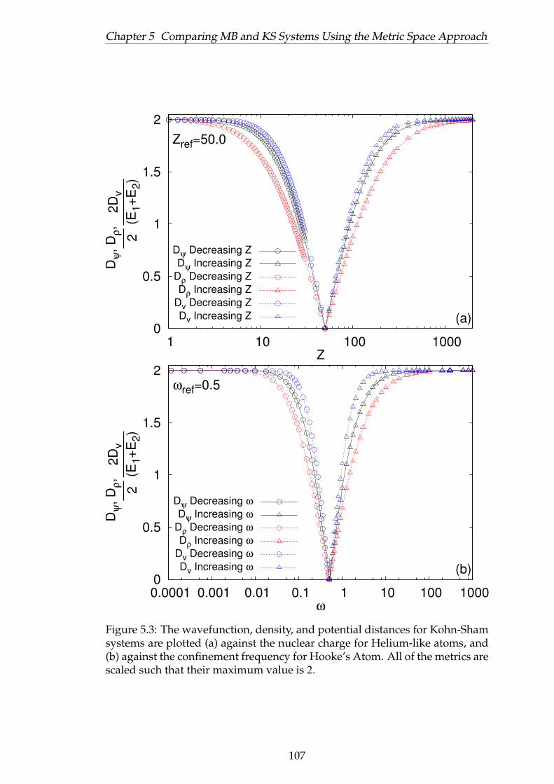
Chapter 5 Comparing MB and KS Systems Using the Metric Space Approach
0
0.5
1
1.5
2
1 10 100 1000Z
Zref=50.0
(a)
Dψ Decreasing ZDψ Increasing Z
Dρ Decreasing ZDρ Increasing Z
Dv Decreasing ZDv Increasing Z
0
0.5
1
1.5
2
0.0001 0.001 0.01 0.1 1 10 100 1000ω
ωref=0.5
(b)
Dψ Decreasing ωDψ Increasing ω
Dρ Decreasing ωDρ Increasing ω
Dv Decreasing ωDv Increasing ω
ρ,2D
v(E
1+E
2)
Dψ,D
2ρ,
2Dv
(E1+
E2)
Dψ,D
2
Figure 5.3: The wavefunction, density, and potential distances for Kohn-Shamsystems are plotted (a) against the nuclear charge for Helium-like atoms, and(b) against the confinement frequency for Hooke’s Atom. All of the metrics arescaled such that their maximum value is 2.
107

Chapter 5 Comparing MB and KS Systems Using the Metric Space Approach
5.5 Determining the Distances between Correspond-
ing Many-Body and Kohn-Sham Quantities
Finally, we will use our metrics to determine the distance between the wave-functions and potentials used in the many-body picture, and those used todescribe the same system in the Kohn-Sham picture.1 For the first time, weare able to provide a quantitative description of the differences between themany-body and exact Kohn-Sham descriptions of quantum systems.
In Fig. 5.4, the distances between many-body and Kohn-Sham wavefunctionsand potentials are plotted for a range of parameter values. We firstly observethat the wavefunction and potential distances always take approximately thesame value throughout the parameter range explored for both systems. Thisdemonstrates that the two metrics provide a consistent measure of how themany-body description differs from the Kohn-Sham description of our sys-tems. For both systems we have also plotted the ratio of the expectation valueof the Coulomb operator to the expectation value of the external potential op-erator. This ratio can be seen to follow broadly the the same trend as the met-rics. This is an important observation as it provides further confirmation thatthe metrics derived from the metric space approach to quantum mechanicsprovide a physically relevant comparison of quantum mechanical functions.It also shows that, alongside the two metrics, this ratio is a useful measure ofhow much the many-body and Kohn-Sham descriptions of the system differfrom one another.
For Helium-like atoms, we observe that the many-body and Kohn-Sham de-scriptions of the system are always relatively similar across the parameterrange studied, with the distances between the quantities decreasing monoton-ically as Z increases. For this system, the external potential always dominatesover the Coulomb interaction between the electrons. We also observe that thedistance between the potentials is always larger than the distance between thewavefunctions.
For Hooke’s atom, we consider three regimes: large values of ω0, where the ex-ternal potential dominates over the Coulomb interaction; intermediate valuesof ω0, where the external potential and Coulomb interaction make comparablecontributions; and small values of ω0, where the Coulomb interaction domi-nates over the external potential. For small and large values of ω0, we observethat the value of the potential metric is greater than that of the wavefunctionmetric. However, in the region where the ratio is approximately unity, the
1For densities, it is required that Dρ (ρMB,ρKS)≡ 0.
108

Chapter 5 Comparing MB and KS Systems Using the Metric Space Approach
0
0.1
0.2
0.3
0.4
1 10 100Z
(a)
Wavefunction distancePotential Distance
<U>/<V>Dψ,
,<U>/<V>
2Dv
(E1+E2)
0
0.5
1
1.5
2
1e-08 1e-06 0.0001 0.01 1 100ω
(b)
Wavefunction distancePotential Distance
<U>/<V>
0
0.2
0.4
0.1 1 10 1001000
Dψ,
,<U>/<V>
2Dv
(E1+E2)
Figure 5.4: For (a) Helium-like atoms and (b) Hooke’s Atom, the distances be-tween many-body and Kohn-Sham wavefunctions, and between many-bodyand Kohn-Sham potentials, are plotted against the parameter values. In ad-dition, the ratio of the expectation of the electron-electron interaction to themany-body external potential energy is plotted and shown to follow a similartrend to the metrics. In the inset, we focus on Hooke’s Atom in the regime ofdistances covered by the Helium-like atoms.
109
Chapter 5 Comparing MB and KS Systems Using the Metric Space Approach
wavefunction metric takes a larger value than the potential metric.
Physically, the values of the wavefunction and potential metrics for the dis-tances between many-body and Kohn-Sham systems can be interpreted as ameasure of the electron-electron interaction effects. Specifically, the Kohn-Sham wavefunction is the product of single particle states, hence the wave-function distance can be interpreted as a measure of the features present inthe many-body wavefunction that go beyond single particle approximations.For potentials, the Kohn-Sham potential is composed of three components:the external potential used for the many-body description, the Hartree poten-tial and the exchange-correlation potential. Therefore, the value of the metricDV (Vext ,VKS) can be interpreted as measuring the contribution of the Hartreeand exchange-correlation potentials to the Kohn-Sham potential.
The results in this Chapter provide us with a new perspective on Kohn-ShamDFT. Previous studies comparing many-body and Kohn-Sham (either exactor approximated) quantities have either made qualitative statements [82, 106,107], or identified features of Kohn-Sham quantities [71, 108, 109]. With ourmetrics, we have a well-defined numerical value that gives a simple descrip-tion of how different the many-body and Kohn-Sham descriptions of a quan-tum system are. This measure is an important addition to the range of toolsused to explore the Kohn-Sham picture. When developing functionals andapproximations for DFT, our metrics can be used in order to quantify howclosely they reproduce the exact KS quantities, and how they compare to otherapproximations. In addition, the fact that, for the systems studied, the ratio ofthe Coulomb interaction between the electrons to the external potential closelymirrors the values of the metrics is a significant result. Although further anal-ysis is required to see if this result holds for more complex systems, this ra-tio, which is relatively simple to approximate for many systems, could poten-tially give users of DFT an indication of the significance of Hartree-exchange-correlation effects, and, consequently, could act as a guide as to which approx-imation to Vxc is most appropriate for the system studied.
110

Chapter 6
Conclusions
In this thesis, we have developed and applied the metric space approach toquantum mechanics, which is a new method to derive physically relevantmetrics for quantum mechanical functions. We have applied the approachto study many-body quantum mechanics, specifically by considering DensityFunctional Theory (DFT) and Current Density Functional Theory (CDFT), andin doing so have gained additional insight into the fundamental nature of thesetheories.
In Chapter 1, we introduced the theory of quantum mechanics, drew atten-tion to the significance of conservation laws in developing theoretical physics,and proved various conservation laws in quantum mechanics. We then out-lined the many-body problem in quantum mechanics and introduced one ofthe main approaches employed in order to tackle it, namely DFT. We discussedthe Hohenberg-Kohn theorem and the Kohn-Sham scheme, highlighting thatboth of these fundamental elements of DFT draw connections between dif-ferent quantum mechanical functions, and are therefore amenable to studiesinvolving comparisons between these functions. We then introduced the con-cept of a metric space, and showed the connection between vector spaces andquantum mechanics. Finally, we examined previous work in the literature thatapplied metric spaces to quantum mechanical functions.
The fundamental theory behind the metric space approach to quantum me-chanics was set out in Chapter 2. We argued that the best choice of metricfor studying quantum mechanical functions is one that captures fundamentalphysics at its core, and for this reason we chose to base our metrics on con-servation laws. Another highly significant advantage of developing metricsfrom conservation laws is that we demonstrated a straightforward, generalmethod to derive metrics from integral, or sum, conservation laws. These met-rics were shown to possess an “onion-shell” geometry consisting of concentric
111

Chapter 6 Conclusions
spheres, that allows us to visualise the metric spaces. We then applied the met-ric space approach to generate metrics for specific quantum mechanical func-tions: wavefunctions, particle densities, paramagnetic current densities, andscalar potentials. All of these quantities can be linked to quantum mechanicalconservation laws, and are fundamentally important for DFT and CDFT.
We also demonstrated the extensions to the metric space approach that enablethe theory to be applied to a wider range of functions. For wavefunctions,we showed how equivalence classes can be defined in order to restrict the de-rived metric to wavefunctions that correspond to different physical situations,ensuring that wavefunctions that differ by a trivial phase factor are assignedzero distance. Equivalence classes were also utilised in order to associate themetric derived from the z-component of angular momentum to the transversecomponent of the paramagnetic current density. In this case the equivalenceclasses were directly induced by the conservation law. In addition, we showedthat the gauge variant paramagnetic current density can be associated with agauge invariant current density. This enables the paramagnetic current den-sity metric to be used in all gauges. All of these measures have ensured thatthe metrics we define are gauge invariant.
Having established the physical and mathematical framework of the metricspace approach to quantum mechanics, the approach was then used to gain adeeper insight into CDFT. Specifically, we calculated the wavefunctions, par-ticle densities and paramagnetic current densities of two different model sys-tems, generating a family of states by varying a single parameter in the Hamil-tonian. Applying our metrics to each of these quantities allowed us to comparethe distances between ground-state wavefunctions, and their correspondingparticle densities and paramagnetic current densities; and to study the uniquerelationship between these three variables defined in CDFT. In Chapter 3, weconsidered variations in the potential energy, firstly by changing the strengthof the harmonic confining potential for the Magnetic Hooke’s Atom and theInverse Square Interaction (ISI) system and then the strength of the electron-electron interaction for the ISI system. We considered the relationships be-tween each of the three metrics; the relationship between the wavefunctionand particle density metrics was found to bear a close resemblence to thatfound for systems without magnetic fields in Ref. [58]. Specifically, we onceagain observe a monotonic relationship, which is linear for low to intermediatedistances, and the curves for increasing and decreasing confinement strengthoverlapping one another. However, the application of a magnetic field causeda significant feature to emerge for ground state metric spaces – the “bandstructure” of allowed (“bands”) and forbidden (“gaps”) distances, caused by
112
Chapter 6 Conclusions
changes in the angular momentum quantum number, m. When consideringthe “onion-shell” geometry of our metric spaces, we observed that paramag-netic current densities “jump” from one sphere to another when the value of m
changes, and as such we can determine the angular width of each of the bandsin this metric space. It was found that the bands moved from the north pole ofthe sphere to the south pole as we departed from the reference value of m, andthat the width of the bands decreased as m increased.
In Chapter 4, the analysis of the metrics and their interrelationships was ex-tended to encompass variations in the magnetic field, and we examined howthe “band structure” arising from the presence of the magnetic field respondedto changes in the field. The principal result of this analysis was the emergenceof “overlapping bands” in the metric spaces for ground state wavefunctionsand particle densities, resulting in a lack of forbidden distances for these quan-tities. We also used our metrics in order to gain an insight into the uniquerelationship between wavefunctions, particle densities, and paramagnetic cur-rent densities in CDFT by examining the ratio of the metrics for paramagneticcurrent densities and particle densities, where we found that there was a starkdifference between the situations where m = mre f , and m 6= mre f . When con-sidering functions with the same value of m, the ratio of paramagnetic currentdensity and particle density metrics was seen to be constant, but this was notthe case for functions with different values of m. We then extended our analysisbeyond CDFT to consider excited states. In this case, when considering differ-ent values of m, the curves for wavefunctions and particle densities were seento collapse on to one another, but this was not the case when paramagneticcurrent densities were considered. Examining again the ratio of paramagneticcurrent density and particle density metrics, the constant relationship for equalvalues of m was seen to persist up to fairly large wavefunction distances. All ofthese findings indicate that changes in m are very significant when modellingsystems subject to magnetic fields.
Chapter 5 was concerned with the Kohn-Sham scheme of ground-state DFT,and extending the analysis of the Hohenberg-Kohn theorem using the metricfor potentials. The relationship between the external potential and the wave-function was seen to share many characteristics with the relationship betweenwavefunctions and densities, principally the monotonic relationship that in-corporates a linear region. We observed that the extent of this linear regionwas different depending on which two metrics were considered. With threemetrics now available for characterising many-body systems, we analysed theperformance of each of them, and found that the density metric is more usefulfor comparing systems at large distances, as this metric will provide non-trivial
113

Chapter 6 Conclusions
information about these systems. Finally, we studied the distances betweencorresponding many-body and Kohn-Sham systems in order to quantify howdifferent the many-body interacting and Kohn-Sham descriptions of quantumsystems are. We found that both wavefunctions and potentials gave comple-mentary results, showing the same qualitative picture and a similar quantita-tive picture throughout the parameter space explored. For the model systemsstudied, we also found that the ratio of the expectation of the electronic pair-wise Coulomb interaction to that of the potential energy followed the samequalitative trend as the metrics.
Overall, the metric space approach to quantum mechanics has enabled us toexamine quantum mechanics beyond the wavefunction. This has been achievedby constructing metric spaces for a range of quantum mechanical functions,allowing all of them to be treated on an equal footing. DFT is a particularlyuseful illustration of the metric space approach, since the fundamental tenet ofDFT is to move from the Hilbert space of wavefunctions to the set of densities,which does not form a vector space. When applied to relationships fundamen-tal to DFT and CDFT, our approach has revealed distinctive signatures suchas: monotonicity, (piecewise) linearity, and “band structures”, that go beyondwhat is defined by the theories. Our metrics also provide quantitative, physi-cally meaningful information when comparing quantum systems. Hence, theycould enhance the development of approaches to quantum modelling, andprovide a physically relevant way to assess the construction of approxima-tions to quantum mechanical functions. The results in this thesis suggest thatthe metric space approach to quantum mechanics is a powerful tool to studyquantum systems governed by conservation laws.
6.1 Future Work
Having established the formalism of the metric space approach to quantummechanics, there are many possible applications and directions for future re-search. We have primarily considered DFT and CDFT in this thesis, but ourapproach is easily applicable to the study of quantum mechanical functions inorder to gain insight into quantum phenomena and other approaches used tomodel quantum systems. Although most of the research in this thesis has beenconcerned with systems in the ground state, in Chapter 4 we showed that themetric space approach to quantum mechanics can be easily applied to excitedstates. Given that there are fewer approaches to modelling systems in excitedstates compared to ground states, the metric space approach could prove use-ful in improving the understanding of excited state properties.
114

Chapter 6 Conclusions
One example of a theory that provides insight into excited states, and on whicha significant amount of research is currently underway, is time-dependent DFT(TDDFT). The metric space approach may also be able to provide insight intothis rapidly developing theory. In TDDFT, the Runge-Gross theorem states thatthe many-body wavefunction and potential at a particular time are uniquelydetermined by the density at the current time and all previous times, alongwith the initial wavefunction of the system [37]. TDDFT also defines a versionof the Kohn-Sham scheme for time-dependent systems. Our metrics for wave-functions and densities are immediately applicable in the time-dependent case,and thus the metric space approach to quantum mechanics could be appliedto gain insight into the relationships between many-body wavefunctions anddensities, as defined by the Runge-Gross theorem, and many-body and Kohn-Sham quantities. These relationships can be studied at particular points intime, and we can also use our metrics to quantify how much wavefunctionsand densities evolve in time.
The most significant result from our studies of CDFT is the presence of the“band structure” in ground-state metric spaces. It would be worthwhile toexplore a greater range of systems in order to establish how universal this fea-ture is, and whether changes in the value of m continue to carry significance.A metric-space-based analysis of the non-uniqueness problem may providesome interesting insights, particularly since this problem is one of the biggestissues curtailing practical implementation of CDFT. However, there are somechallenges; in particular we do not have a metric for the vector potential, andour metric for scalar potentials applies only to systems where A(r) = 0. If theseissues could be overcome, it would be interesting to take a range of potentialsthat map to the same wavefunction, and compare the distances between them.The values of distances between scalar and vector potentials and the relation-ship between these distances could both provide a much greater insight intothe non-uniqueness problem.
The fact that the ratio of Coulomb interaction energy to external potential en-ergy closely follows the values of the distances between many-body and Kohn-Sham systems is an intriguing result that is worthy of further consideration. Itwould be interesting to see if this result continues to hold for a wider variety ofsystems than those studied in this thesis. Also, as it has been indicated that thismeasure of interaction is not applicable for non-monotonic potentials [110], itwould also be interesting to see how other proposed measures compare to themetrics in these cases, and whether or not measures of interaction are a suit-able way to estimate how the many-body picture differs from the Kohn-Shampicture for the system under consideration.
115

Chapter 6 Conclusions
A natural, and promising, extension to the calculations of distances betweenmany-body and Kohn-Sham systems in Chapter 5 would be to consider thewavefunctions, densities, and potentials arising from approximations in DFTand TDDFT, and hence use the metric space approach to quantum mechanicsin order to quantify the performance of these approximations. For model sys-tems like the ones studied in this thesis, our metrics could be used to measurehow much the wavefunctions and potentials corresponding to approximationssuch as the local density approximation [24] differ from those used in the exactKohn-Sham description. For more complex systems where the exact Kohn-Sham quantities cannot be obtained, the metrics could still be useful in orderto compare approximations with one another, which can help to determine re-gions of parameter space where certain approximations may perform betterthan others for the system considered. This analysis could also be performedin order to guide the development of new approximations.
116
Appendix A
Determining the Gauges where Lz isa Constant of Motion
In order to be a constant of motion, the z-component of the angular momen-tum Lz =−i [r×∇]z must commute with the Hamiltonian. Given that a vectorpotential is present, we consider the Pauli Hamiltonian
H =−12
∇2− i
2(A ·∇+∇ ·A)+
12
A2 +V (r) , (A.1)
with V (r) such that[V (r) , Lz
]= 0. The Hamiltonian Eq. (A.1) does not neces-
sarily commute with Lz for a particular A(r), because Lz is gauge variant. Forinstance, Lz commutes with the Hamiltonian Eq. (A.1) in the symmetric gaugeA = [y,−x,0] and does not commute with it in the Landau gauge A = [0,−x,0].We wish to determine the general set of vector potentials where
[H, Lz
]= 0.1
A.1 Simplifying the Commutator
The commutator we wish to evaluate is:
[H, Lz
]=− i
[A ·∇
(x
∂ψ
∂y
)−A ·∇
(y
∂ψ
∂x
)− x
∂
∂y(A ·∇ψ)+ y
∂
∂x(A ·∇ψ)
+∇ ·(
Ax∂ψ
∂y
)−∇ ·
(Ay
∂ψ
∂x
)− x
∂
∂y∇ · (Aψ)+ y
∂
∂x∇ · (Aψ)
]+A2x
∂ψ
∂y−A2y
∂ψ
∂x− x
∂
∂y
(A2
ψ)+ y
∂
∂x
(A2
ψ), (A.2)
1In the case where we have many-body interactions, we only consider the case[U (ri,r j) , Lz
]= 0, as is the case for the Coulomb interaction.
117

Appendix A Determining the Gauges where Lz is a Constant of Motion
where we have used that[−1
2∇2 +V (r) , Lz]= 0. We will impose the condition[
H, Lz]= 0, and then solve the commutator to obtain the vector potential A.
Eq. (A.2) reduces to
[H, Lz
]=− i
[A ·(
x∇∂ψ
∂y
)+A ·
(∂ψ
∂y∇x)−A ·
(y∇
∂ψ
∂x
)−A ·
(∂ψ
∂x∇y)
−2x∂
∂y(A ·∇ψ)+2y
∂
∂x(A ·∇ψ) ,
+∇ ·(
Ax∂ψ
∂y
)−∇ ·
(Ay
∂ψ
∂x
)− x
∂
∂y(ψ∇ ·A)+ y
∂
∂x(ψ∇ ·A)
]− xψ
∂A2
∂y+ yψ
∂A2
∂x= 0.
We now perform the vector operations. For compactness, we use a notationri = r1,r2,r3 = x,y,z, which gives,
[H, Lz
]=
3
∑i=1
−i[
Aix∂
∂ ri
∂ψ
∂y+Ai
∂ψ
∂y∂x∂ ri−Aiy
∂
∂ ri
∂ψ
∂x−Ai
∂ψ
∂x∂y∂ ri
−2x∂
∂y
(Ai
∂ψ
∂ ri
)+2y
∂
∂x
(Ai
∂ψ
∂ ri
)+
∂
∂ ri
(Aix
∂ψ
∂y
)− ∂
∂ ri
(Aiy
∂ψ
∂x
)− x
∂
∂y
(ψ
∂Ai
∂ ri
)+ y
∂
∂x
(ψ
∂Ai
∂ ri
)]−xψ
∂A2
∂y+ yψ
∂A2
∂x
,
=3
∑i=1
−i[−xAi
∂
∂ ri
∂ψ
∂y−2x
∂ψ
∂ ri
∂Ai
∂y+2Ai
∂ψ
∂y∂x∂ ri
+ yAi∂
∂ ri
∂ψ
∂x+2y
∂ψ
∂ ri
∂Ai
∂x
−2Ai∂ψ
∂x∂y∂ ri
+Aiy∂ψ
∂y∂x∂ ri
+ xAi∂
∂ ri
∂ψ
∂y+ x
∂ψ
∂y∂Ai
∂ ri−Ai
∂ψ
∂x∂y∂ ri− yAi
∂
∂ ri
∂ψ
∂x
−xψ∂
∂y∂Ai
∂ ri− x
∂Ai
∂ ri
∂ψ
∂y+ yψ
∂
∂x∂Ai
∂ ri+ y
∂Ai
∂ ri
∂ψ
∂x
]−xψ
∂A2
∂y+ yψ
∂A2
∂x
,
=3
∑i=1
−i[
2Ai
(∂ψ
∂y∂x∂ ri− ∂ψ
∂x∂y∂ ri
)−2x
∂ψ
∂ ri
∂Ai
∂y+2y
∂ψ
∂ ri
∂Ai
∂x− xψ
∂
∂y∂Ai
∂ ri+ yψ
∂
∂x∂Ai
∂ ri
]−xψ
∂A2
∂y+ yψ
∂A2
∂x
= 0.
118

Appendix A Determining the Gauges where Lz is a Constant of Motion
Writing this out explicitly, we obtain
− i[(
2Ax∂ψ
∂y−2Ay
∂ψ
∂x
)−2x
(∂ψ
∂x∂Ax
∂y+
∂ψ
∂y∂Ay
∂y+
∂ψ
∂ z∂Az
∂y
)+2y
(∂ψ
∂x∂Ax
∂x+
∂ψ
∂y∂Ay
∂x+
∂ψ
∂ z∂Az
∂x
)− xψ
∂
∂y
(∂Ax
∂x+
∂Ay
∂y+
∂Az
∂ z
)+yψ
∂
∂x
(∂Ax
∂x+
∂Ay
∂y+
∂Az
∂ z
)]− xψ
∂A2
∂y+ yψ
∂A2
∂x= 0. (A.3)
In order to progress with the solution of this equation, we first consider thecase where ψ, ∂ψ
∂x ,∂ψ
∂y and ∂ψ
∂ z are all independent of each other. This choiceallows us to decompose Eq. (A.3) into a set of simultaneous equations, whichwe can then solve. The solution of these equations will provide properties ofthe general set of vector potentials where
[H, Lz
]= 0. Using these properties,
we will then solve Eq. (A.3) for A(r) using a general wavefunction.
With our choice of trial wavefunction, we write the set of simultaneous equa-tions
ix∂
∂y
(∂Ax
∂x+
∂Ay
∂y+
∂Az
∂ z
)− x
∂A2
∂y− iy
∂
∂x
(∂Ax
∂x+
∂Ay
∂y+
∂Az
∂ z
)+ y
∂A2
∂x= 0,
(A.4)
Ay + x∂Ax
∂y− y
∂Ax
∂x= 0, (A.5)
Ax− x∂Ay
∂y+ y
∂Ay
∂x= 0, (A.6)
y∂Az
∂x− x
∂Az
∂y= 0. (A.7)
We concentrate first on Eqs. (A.5)-(A.7), a set of three equations for the threeunknowns Ax, Ay and Az. Firstly, we consider Eq. (A.7). In order to solve thispartial differential equation (PDE), we use the method of characteristics [111].
The method of characteristics requires the visualisation of Eq. (A.7) in 4D co-ordinates (x,y,z,u). By considering the solution surface u = Az (x,y,z), we canwrite
Az (x,y,z)−u = 0.
For any surface, S, a normal vector to the surface is given by ∇S. Thus, thevector
[∂Az∂x ,
∂Az∂y ,
∂Az∂ z ,−1
]is normal to the solution surface. We now write the
PDE (A.7) as a scalar product
[y,−x,0,0] ·[
∂Az
∂x,∂Az
∂y,∂Az
∂ z,−1
]= 0.
Since the scalar product of these two vectors is zero, they must be orthogo-
119

Appendix A Determining the Gauges where Lz is a Constant of Motion
nal. Given also that the vector[
∂Az∂x ,
∂Az∂y ,
∂Az∂ z ,−1
]is normal to the surface, this
tells us that the vector field [y,−x,0,0] is tangent to the surface at every point,providing a geometrical interpretation of the PDE. Thus, any curve withinthe surface Az (x,y,z)− u = 0 that has the vector [y,−x,0,0] as a tangent at ev-ery point must lie entirely within the surface. Such curves are called char-acteristic curves [111]. Any curve can be described by a parameter, t, andthe tangent of such a curve, r(t), is given by the derivative with respect tothis parameter r′ (t). Therefore, the tangent of a characteristic curve, r(t) =[x(t) ,y(t) ,z(t) ,Az (t)], is given by the vector
r′ (t) =[
dxdt
,dydt
,dzdt
,dAz
dt
].
This vector is therefore proportional to the tangent vector [y,−x,0,0] for thischaracteristic curve, allowing us to construct the equations
dxdt
= y, (A.8)
dydt
=−x, (A.9)
dzdt
= 0, (A.10)
dAz
dt= 0. (A.11)
These are the characteristic equations of the PDE (A.7).
Solving this set of ordinary differential equations (ODEs) yields the solution ofthe original PDE (A.7), since
dAz
dt=
dxdt
∂Az
∂x+
dydt
∂Az
∂y+
dzdt
∂Az
∂ z,
= y∂Az
∂x− x
∂Az
∂y= 0.
By eliminating the parameter t in Eqs. (A.8)-(A.11), we can reduce the set ofODEs to three equations
dydx
=−xy, (A.12)
dzdx
= 0, (A.13)
dAz
dx= 0. (A.14)
We now note that the “constant” of integration in Eq. (A.14) has a functionaldependence on the solutions to Eqs. (A.12) and (A.13). This is because the
120

Appendix A Determining the Gauges where Lz is a Constant of Motion
ODEs are solved along characteristic curves; the constants of integration areconstant along a particular characteristic, but can vary between characteristics.The solutions to Eqs. (A.12) and (A.13) are
x2 + y2 = a, z = b, (A.15)
respectively, where a and b are the constants of integration. Thus, the solutionfor Az is
Az = γ(x2 + y2,z
), (A.16)
where γ is an arbitrary function.
A.2 Solving the Simultaneous Equations
We will now solve Eqs. (A.5) and (A.6) simultaneously. Firstly, we differentiateEq. (A.5) with respect to both x and y which gives:
∂Ay
∂x+
∂Ax
∂y+ x
∂ 2Ax
∂x∂y− y
∂ 2Ax
∂x2 = 0, (A.17)
∂Ay
∂y+ x
∂ 2Ax
∂y2 −∂Ax
∂x− y
∂ 2Ax
∂x∂y= 0, (A.18)
respectively. Now, we substitute these expressions for ∂Ay∂x and ∂Ay
∂y into Eq. (A.6),and obtain
Ax− x(−x
∂ 2Ax
∂y2 +∂Ax
∂x+ y
∂ 2Ax
∂x∂y
)+ y(−∂Ax
∂y− x
∂ 2Ax
∂x∂y+ y
∂ 2Ax
∂x2
)= 0, (A.19)
y2 ∂ 2Ax
∂x2 −2xy∂ 2Ax
∂x∂y+ x2 ∂ 2Ax
∂y2 − x∂Ax
∂x− y
∂Ax
∂y+Ax = 0. (A.20)
We now have an equation containing only the unknown Ax that we can solve.
We begin to solve this equation by again using the method of characteristics.For second order PDEs, it is firstly necessary to determine the type of equation,either hyperbolic, parabolic or elliptic. This is done by calculating the discrim-inant b2− 4ac, where a,b,c are the coefficients of ∂ 2Ax
∂x2 ,∂ 2Ax∂x∂y ,
∂ 2Ax∂y2 respectively.
This will then allow us to perform an appropriate change of variables from(x,y,z) to (ξ ,η ,z), where ξ and η are the characteristics [81]. The discriminantis
b2−4ac = 4x2y2−4x2y2 = 0. (A.21)
Therefore, the characteristic equation is parabolic and has one repeated solu-
121
Appendix A Determining the Gauges where Lz is a Constant of Motion
tion, which we take for ξ . The characteristic equation is the ODE [81]
y2(
dydx
)2
−2xydydx
+ x2 = 0, (A.22)
solving for dydx gives
dydx
=−xy.
Hence, from Eq. (A.15), we know that the first characteristic is ξ = a = x2 + y2.Since there is only one root of the characteristic equation, we have completefreedom in the choice for η , provided that it is not the same as ξ . Given thatwe know that the symmetric gauge satisfies the commutator
[H, Lz
]= 0, and,
specifically, that Ax = y is a solution for Eq. (A.20), we choose η = y. By usingthe chain rule, we find the derivatives in Eq. (A.20).
∂Ax
∂x= 2x
∂Ax
∂ξ,
∂Ax
∂y= 2y
∂Ax
∂ξ+
∂Ax
∂η,
∂ 2Ax
∂x2 = 4x2 ∂ 2Ax
∂ξ 2 +2∂Ax
∂ξ,
∂ 2Ax
∂y2 = 4y2 ∂ 2Ax
∂ξ 2 +4y∂ 2Ax
∂ξ ∂η+
∂ 2Ax
∂η2 +2∂Ax
∂ξ,
∂ 2Ax
∂x∂y= 4xy
∂ 2Ax
∂ξ 2 +2x∂ 2Ax
∂ξ ∂η.
Substituting into equation (A.20), we get
4x2y2 ∂ 2Ax
∂ξ 2 +2y2 ∂Ax
∂ξ−8x2y2 ∂ 2Ax
∂ξ 2 −4x2y∂ 2Ax
∂ξ ∂η+4x2y2 ∂ 2Ax
∂ξ 2 +4x2y∂ 2Ax
∂ξ ∂η,
+ x2 ∂ 2Ax
∂η2 +2x2 ∂Ax
∂ξ−2x2 ∂Ax
∂ξ−2y2 ∂Ax
∂ξ− y
∂Ax
∂η+Ax = 0,
x2 ∂ 2Ax
∂η2 − y∂Ax
∂η+Ax = 0,
and completing the change of variables gives
(ξ −η
2) ∂ 2Ax
∂η2 −η∂Ax
∂η+Ax = 0. (A.23)
We have now completed a change of variables and reduced the complexity ofthe equation. The next step is to perform a reduction of order through the use
122

Appendix A Determining the Gauges where Lz is a Constant of Motion
of the known solution Ax = η . The reduction used is
Ax = uη ,∂Ax
∂η= η
∂u∂η
,∂ 2Ax
∂η2 = η∂ 2u∂η2 +2
∂u∂η
,
which we substitute into Eq. (A.23) to give
(ξ −η
2)(η
∂ 2u∂η2 +2
∂u∂η
)−η
2 ∂u∂η−ηu+ηu = 0,
η(ξ −η
2) ∂ 2u∂η2 +
(2ξ −3η
2) ∂u∂η
= 0. (A.24)
We now make the substitution v = ∂u∂η
, obtaining
η(ξ −η
2) ∂v∂η
+(2ξ −3η
2)v = 0. (A.25)
This equation can now be solved separably,
∫ 1v
dv =∫ [ 3η2−2ξ
η (ξ −η2)
]dη .
We decompose the denominator through the use of partial fractions, giving,
3η2−2ξ
η (ξ −η2)=
Iη+
Jη +Kξ −η2 ,
=I(ξ −η2)
η (ξ −η2)+
(Jη +K)η
η (ξ −η2),
3η2−2ξ = I
(ξ −η
2)+ Jη2 +Kη .
By comparing coefficients, we see that K = 0, −I + J = 3⇒ I =−2, J = 1,
3η2−2ξ
η (ξ −η2)=− 2
η+
η
ξ −η2 .
123
Appendix A Determining the Gauges where Lz is a Constant of Motion
Returning to the solution of equation (A.25), we find
∫ 1v
dv =−∫ 2
ηdη +
∫η
ξ −η2 dη ,
=−∫ 2
ηdη− 1
2
∫ −2η
ξ −η2 dη ,
lnv =−2lnη− 12
ln∣∣ξ −η
2∣∣+ ln [α (ξ )],
= lnη−2 + ln
(ξ −η
2)− 12 + ln [α (ξ )],
= ln
[α (ξ )
η2 (ξ −η2)12
],
v =α (ξ )
η2 (ξ −η2)12,
where α is an arbitrary function, and we note that ξ −η2 = x2+y2−y2 = x2 > 0,hence, ξ −η2 is always positive.
Now that we have a solution to (A.25), we must reverse our substitutions toget a solution for Ax. Firstly, we integrate v to get u,
u = α (ξ )∫ 1
η2 (ξ −η2)12
dη . (A.26)
We make the substitution η = ξ12 sinθ ,
u = ξ12 α (ξ )
∫ cosθ
ξ sin2θ(ξ −ξ sin2
θ) 1
2dθ ,
= ξ12 α (ξ )
∫ cosθ
ξ sin2θ (ξ cos2 θ)
12
dθ ,
=α (ξ )
ξ
∫ 1sin2
θdθ ,
=−α (ξ )
ξcotθ +β (ξ ) ,
=−α (ξ )
ξcot
[sin−1
(η
ξ12
)]+β (ξ ) ,
=−α (ξ )
ξ
ξ12
η
(1− η2
ξ
) 12
+β (ξ ) ,
=−α (ξ )
ξ η
(ξ −η
2) 12 +β (ξ ) ,
124

Appendix A Determining the Gauges where Lz is a Constant of Motion
where β is another arbitrary function. Next, we write Ax = uη , obtaining
Ax = α (ξ )(ξ −η
2) 12 +ηβ (ξ ) , (A.27)
where we absorb the factor of − 1ξ
into α . Finally, we substitute back from(ξ ,η ,z) to (x,y,z),
Ax = α(x2 + y2,z
)(x2 + y2− y2) 1
2 + yβ(x2 + y2,z
),
= xα(x2 + y2,z
)+ yβ
(x2 + y2,z
), (A.28)
to give the solution for Ax. We find Ay from equation (A.5),
Ay =y∂Ax
∂x− x
∂Ax
∂y,
=y[α(x2 + y2,z
)+2x2
α′ (x2 + y2,z
)+2xyβ
′ (x2 + y2,z)]
− x[2xyα
′ (x2 + y2,z)+β
(x2 + y2,z
)+2y2
β′ (x2 + y2,z
)],
=yα(x2 + y2,z
)− xβ
(x2 + y2,z
),
giving us solutions for all three components.
We will now verify that the solutions for Ax,Ay,Az, satisfy the remaining equa-tion, Eq. (A.4)
ix∂
∂y
(∂Ax
∂x+
∂Ay
∂y+
∂Az
∂ z
)− x
∂A2
∂y− iy
∂
∂x
(∂Ax
∂x+
∂Ay
∂y+
∂Az
∂ z
)+ y
∂A2
∂x
=ix∂
∂y
(2α +2x2
α′+2xyβ
′+2y2α′−2xyβ
′+∂γ
∂ z
)− iy
∂
∂x
(2α +2x2
α′+2xyβ
′+2y2α′−2xyβ
′+∂γ
∂ z
)− x(4x2yαα
′+2yβ2 +4y3
ββ′+2yα
2 +4y3αα′+4x2yββ
′+4yγγ′)
+ y(2xα
2 +4x3αα′+4xy2
ββ′+4xy2
αα′+2xβ
2 +4x3ββ′+4xγγ
′) ,=i(
4xyα′+4xyα
′+4x3yα′′+4xy3
α′′+2xy
∂γ ′
∂ z
−4xyα′−4x3yα
′′−4xyα′−4xy3
α′′−2xy
∂γ ′
∂ z
)= 0,
where a prime denotes differentiation with respect to(x2 + y2).
Therefore, the form of the vector potential required for[H, Lz
]= 0 is,
A =[xα(x2 + y2,z
)+ yβ
(x2 + y2,z
),yα
(x2 + y2,z
)− xβ
(x2 + y2,z
),γ(x2 + y2,z
)],
(A.29)
125

Appendix A Determining the Gauges where Lz is a Constant of Motion
or, in cylindrical polar coordinates (r,θ ,z),
A =[rα(r2,z
),−rβ
(r2,z
),γ(r2,z
)]. (A.30)
This form of the vector potential satisfies the condition[H, Lz
]= 0 for wave-
functions with ∂ψ
∂x ,∂ψ
∂y and ∂ψ
∂ z all independent of each other. Clearly, vectorpotentials that are not of the form of Eq. (A.29) do not satisfy the condition.But in order to ensure vector potentials of this form satisfy this condition foran arbitrary wavefunction, we use the properties of the vector potentials tosolve the original commutator Eq. (A.3) for an arbitrary wavefunction. Thisgives
[H, Lz
]ψ =− i
2(xα + yβ )
∂ψ
∂y−2(yα− xβ )
∂ψ
∂x
−2x[(
2xyα′+β +2y2
β′) ∂ψ
∂x+(α +2y2
α′−2xyβ
′) ∂ψ
∂y+2yγ
′∂ψ
∂ z
]+2y
[(α +2x2
α′+2xyβ
′) ∂ψ
∂x+(2xyα
′−β −2x2β′) ∂ψ
∂y+2xγ
′∂ψ
∂ z
]−xψ
∂
∂y
(2α +2x2
α′+2xyβ
′+2y2α′−2xyβ
′+∂γ
∂ z
)+yψ
∂
∂x
(2α +2x2
α′+2xyβ
′+2y2α′−2xyβ
′+∂γ
∂ z
)− xψ
(4x2yαα
′+2yβ2 +4y3
ββ′+2yα
2 +4y3αα′+4x2yββ
′+4yγγ′)
+ yψ(2xα
2 +4x3αα′+4xy2
ββ′+4xy2
αα′+2xβ
2 +4x3ββ′+4xγγ
′) .This simplifies to
[H, Lz
]ψ =ixψ
∂
∂y
(2α +2x2
α′+2y2
α′+
∂γ
∂ z
)− iyψ
∂
∂x
(2α +2x2
α′+2y2
α′+
∂γ
∂ z
),
=i(
4xyα′+4xyα
′+4x3yα′′+4xy3
α′′+2xy
∂γ ′
∂ z
−4xyα′−4x3yα
′′−4xyα′−4xy3
α′′−2xy
∂γ ′
∂ z
),
=0.
Thus, the vector potentials of the form Eq. (A.29) fulfill the condition[H, Lz
]=
0, and, in these gauges, Lz is a constant of motion.
126

Appendix B
Gauge Transformations betweenVector Potentials for which Lz is aConstant of Motion
In Appendix A, we found that[H, Lz
]= 0 only when A(r) is of the form of
Eq. (A.29). We now consider a gauge transformation between two gauges ofthe form of Eq. (A.29). A vector potential of this form gives the magnetic field
B(r) = ∇×A(r) ,
= ∇× [xα + yβ ,yα− xβ ,γ] ,
=
[2yγ′− y
∂α
∂ z+ x
∂β
∂ z,x
∂α
∂ z+ y
∂β
∂ z−2xγ
′,2xyα′−β −2x2
β′−2xyα
′−β −2y2β′],
=
[2yγ′− y
∂α
∂ z+ x
∂β
∂ z,x
∂α
∂ z+ y
∂β
∂ z−2xγ
′,−2β −(2x2 +2y2)
β′].
Since any modification to β would affect the −2β term in the z-componentof B(r), and B(r) must be unchanged by gauge transformations, β must beconstant in a gauge transformation.
A gauge transformation is given by A′ (r) = A(r)+∇χ and takes the form
∇χ = A′ (r)−A(r) ,
= [x∆α + y∆β ,y∆α− x∆β ,∆γ] ,
= [x∆α,y∆α,∆γ] , (B.1)
using that ∆β must be zero. We obtain χ (r) by integrating each of the compo-
127

Appendix B Gauge Transformations between Vector Potentials
nents of the vector ∇χ in Eq. (B.1):
∫x∆αdx =
λ(x2 + y2,z
)2
,∫y∆αdy =
µ(x2 + y2,z
)2
,∫∆γdz = ν
(x2 + y2,z
).
Clearly then, the scalar field χ (r) must be a function χ(x2 + y2,z
).
Finally, we demonstrate that [r× jp]z is unchanged by gauge transformationsbetween gauges of the form Eq. (A.29). The paramagnetic current densitytransforms according to j′p (r) = jp (r)+ρ (r)∇χ
[r× j′p
]z =
r× [jp +ρ (r)∇χ]
z ,
= [r× jp]z +[r×ρ (r)∇χ]z ,
= [r× jp]z +[r×ρ (r)(x∆α,y∆α,∆γ)]z ,
= [r× jp]z +ρ (r)(xy∆α− xy∆α) ,
= [r× jp]z .
So, when we are in any gauge of the form of Eq. (A.29), and when we transformbetween any of these gauges, both Lz and [r× jp]z are unaffected.
128

Appendix C
Evaluation of Densities for ModelSystems
Having solved the Schrodinger equation for our model systems, we must usethe resulting wavefunction in order to determine an expression for the particledensity and, for the magnetic systems, the paramagnetic current density, inorder to study these quantities with the metric space approach to quantummechanics. In this Appendix, we will evaluate the densities for the modelsystems that we study in Chapters 3, 4, and 5.
C.1 Conversion of Coordinates
In time-independent quantum mechanics, the particle density is defined asthe probability of finding one of the particles in the system within the volumeelement dr1 about the point r1, independently of the positions of the other par-ticles [1]. As such the particle density is a function of one of the particle coordi-nates. However, Eqs. (3.25), (3.34) and (5.9) for the ground-state wavefunctionsof the 2D magnetic Hooke’s Atom, ISI system and 3D isotropic, non-magneticHooke’s Atom respectively are in terms of relative motion and centre of masscoordinates, (r,R).
Before we can proceed with the calculation of the densities for these systems,we must therefore make a coordinate transformation. Following the approachof Taut et al. [42], we will write the centre of mass coordinate in terms of therelative motion coordinate and a particle coordinate.
129

Appendix C Evaluation of Densities for Model Systems
θ
2r
R
r1
θ1
r1
r2
θ
r θ
θ1
π-θ2
Figure C.1: The relationship between the vectors R, r2 and r1 and the unit vec-
tors for the r1 and r coordinates in 2D.
C.1.1 Two Dimensions
In two dimensions, the coordinates R, r2 and r1 form a triangle in the plane, as
shown in Fig. C.1. Hence, we can write the coordinate R in terms of the othersusing the cosine rule,
R =
√r2
1 +r2
4− r1r cosθ . (C.1)
When evaluating the paramagnetic current density, we must also be able towrite the unit vectors associated to the relative motion coordinate in terms ofthe unit vectors for the particle coordinate. From Fig. C.1, we can determinethat
r =− cosθ r1 + sinθθ1, (C.2)
θ =cos(
π
2−θ
)r1 + sin
(π
2−θ
)θ1,
=sinθ r1 + cosθθ1. (C.3)
130

Appendix C Evaluation of Densities for Model Systems
R
r1
2r
2r sinθ
2r cosθ
θ
φ
x
Figure C.2: The relationship between the vectors R, r2 and r1 in 3D.
C.1.2 Three Dimensions
The relationships between the vectors R, r2 and r1 in three dimensions are shown
in Fig. C.2. We can determine the length of the line x using the cosine rule,
x2 = r21 +
r2
4sin2
θ − r1r sinθ cosφ . (C.4)
Hence, using Pythagoras’ theorem,
R2 = r21 +
r2
4sin2
θ +r2
4cos2
θ − r1r sinθ cosφ ,
R =
√r2
1 +r2
4− r1r sinθ cosφ . (C.5)
C.2 Two-Dimensional Magnetic Hooke’s Atom
In terms of the particle and relative coordinates, the ground state wavefunctionfor the magnetic Hooke’s Atom is given by,
ψ
(r,
√r2
1 +r2
4− r1r cosθ
)=
1π
√ω
reimθ e−ω
(r21+
r24 −r1r cosθ
)u(r) , (C.6)
using Eq. (3.25) and the fact that this is a 2D system. We will use this form ofthe wavefunction in order to evaluate the particle and paramagnetic currentdensities.
131

Appendix C Evaluation of Densities for Model Systems
C.2.1 Particle Density
We evaluate the particle density of the magnetic Hooke’s Atom using [42],
ρ (r1) = 2∫ ∫ ∣∣∣∣∣ψ
(r,
√r2
1 +r2
4− r1r cosθ
)∣∣∣∣∣2
dr. (C.7)
Inserting Eq. (C.6) into Eq. (C.7) gives,
ρ (r1) =2ω
π2 e−2ωr21
∫∞
0e−
ωr22 |u(r)|2
∫ 2π
0e2ωr1r cosθ dθdr,
=2ω
π2 e−2ωr21
∫∞
0e−
ωr22 |u(r)|2
(∫π
0e2ωr1r cosθ dθ +
∫ 2π
π
e2ωr1r cosθ dθ
)dr,
At this point, we note that the theta integrals define a modified Bessel functionof the first kind. The definition of a modified Bessel function as an integral is[112]
In (z) =1π
∫π
0ezcosθ cos(nθ)dθ . (C.8)
Returning to the density, and after recasting the limits of the second theta inte-gral, we have,
ρ (r1) =2ω
π2 e−2ωr21
∫∞
0e−
ωr22 |u(r)|2
(∫π
0e2ωr1r cosθ dθ +
∫π
0e2ωr1r cos(θ−π)d (θ −π)
)dr,
=2ω
πe−2ωr2
1
∫∞
0e−
ωr22 |u(r)|2 [I0 (2ωr1r)+ I0 (2ωr1r)]dr.
Hence, the particle density of the magnetic Hooke’s Atom is given by,
ρ (r1) =4ω
πe−2ωr2
1
∫∞
0e−
ωr22 |u(r)|2 I0 (2ωr1r)dr, (C.9)
in agreement with Ref. [42].
C.2.2 Paramagnetic Current Density
With the wavefunction for Hooke’s Atom written in terms of the coordinates(r,√
r21 +
r2
4 − r1r cosθ
)in Eq. (C.6), the paramagnetic current density is given
by [42]
jp (r1) =−i∫
[ψ∗∇rψ−ψ∇rψ∗]dr. (C.10)
132

Appendix C Evaluation of Densities for Model Systems
The gradient of the wavefunction is
∇rψ =∂ψ
∂ rr+
1r
∂ψ
∂θθ ,
=1π
√ωe−ωr2
1
[eimθ ∂
∂ r
(e−
ω
4 r2eωr1r cosθ u(r)√
r
)r+
e−ω
4 r2u(r)
r32
∂
∂θ
(eimθ eωr1r cosθ
)θ
],
and evaluating the derivatives gives
∇rψ =1π
√ω
re−ωr2
1 eimθ e−ω
4 r2eωr1r cosθ u(r)×[(
−ωr2
+ ωr1 cosθ +1
u(r)dudr− 1
2r
)r+
(im− ωr1r sinθ)
rθ
], (C.11)
and for the complex conjugate
∇rψ∗ =
1π
√ω
re−ωr2
1 e−imθ e−ω
4 r2eωr1r cosθ u(r)×[(
−ωr2
+ ωr1 cosθ +1
u(r)dudr− 1
2r
)r+
(−im− ωr1r sinθ)
rθ
]. (C.12)
Forming the terms in the integrand of Eq. (C.10), we have,
ψ∗∇rψ =
1π2
ω
re−2ωr2
1 e−ω
2 r2e2ωr1r cosθ u(r)2×[(
−ωr2
+ ωr1 cosθ +1
u(r)dudr− 1
2r
)r+
(im− ωr1r sinθ)
rθ
], (C.13)
and,
ψ∇rψ∗ =
1π2
ω
re−2ωr2
1 e−ω
2 r2e2ωr1r cosθ u(r)2×[(
−ωr2
+ ωr1 cosθ +1
u(r)dudr− 1
2r
)r+
(−im− ωr1r sinθ)
rθ
], (C.14)
Thus, we form the integrand in Eq. (C.10) by subtracting Eq. (C.14) from Eq. (C.13),and get
ψ∗∇rψ−ψ∇rψ
∗ =2imω
π21r2 e−2ωr2
1 e−ω
2 r2e2ωr1r cosθ u(r)2
θ . (C.15)
Equation (C.15) is a vector represented in the relative motion coordinates. Sincewe will integrate over this coordinate, we wish to rewrite Eq. (C.15) in termsof the particle coordinates (r1,θ1). Substituting the unit vector from Eq. (C.3)
133

Appendix C Evaluation of Densities for Model Systems
into Eq. (C.15) gives
ψ∗∇rψ−ψ∇rψ
∗ =2imω
π21r2 e−2ωr2
1 e−ω
2 r2e2ωr1r cosθ u(r)2 (sinθ r1 + cosθθ1
).
(C.16)
Now we have written the integrand in the desired coordinate system, we canevaluate the paramagnetic current density using Eq. (C.10),
jp (r1) =−i∫
∞
0
∫ 2π
0
2imω
π21r
e−2ωr21 e−
ω
2 r2e2ωr1r cosθ u(r)2 (sinθ r1 + cosθθ1
)drdθ ,
=2mω
πe−2ωr2
1
∫∞
0
e−ω
2 r2u(r)2
r1π
∫ 2π
0e2ωr1r cosθ
(sinθ r1 + cosθθ1
)drdθ .
For the first term in the theta integral, we have from tables of integrals [112],
∫ 2π
0e2ωr1r cosθ sinθdθ = 0, (C.17)
and Eq. (C.8) shows that the second term defines a first order modified Besselfunction,
jp (r1) =2mω
πe−2ωr2
1
∫∞
0
e−ω
2 r2u(r)2
r1π
(∫π
0e2ωr1r cosθ cosθdθ +
∫ 2π
π
e2ωr1r cosθ cosθdθ
)θ1dr,
=2mω
πe−2ωr2
1
∫∞
0
e−ω
2 r2u(r)2
r[I1 (2ωr1r)+ I1 (2ωr1r)] θ1dr,
Therefore, the paramagnetic current density for the magnetic Hooke’s Atom isgiven by
jp (r1) = θ14mω
πe−2ωr2
1
∫∞
0
e−ω
2 r2u(r)2 I1 (2ωr1r)
rdr. (C.18)
in agreement with Ref. [42].
C.3 Inverse Square Interaction System
The ground state wavefunction of the Inverse Square Interaction (ISI) system isexpressed in terms of the relative motion coordinate and a particle coordinateas,
ψ
(r,
√r2
1 +r2
4− r1r cosθ
)=
ω
π
√1
Γ(µ +1)
(√ω
2r
)µ
eimθ e−ωr2
4 e−ω
(r2
1+r24 −r1r cosθ
).
(C.19)
134

Appendix C Evaluation of Densities for Model Systems
C.3.1 Particle Density
By substituting Eq. (C.19) into Eq. (C.7), we see that the particle density of theISI system is given by,
ρ (r1) =2(
ω
π
)2 1Γ(µ +1)
(ω
2
)µ
e−2ωr21
∫∞
0r2µe−ωr2
∫ 2π
0e2ωr1r cosθ rdθdr,
=2(
ω
π
)2 1Γ(µ +1)
(ω
2
)µ
e−2ωr21×∫
∞
0r(2µ+1)e−ωr2
(∫π
0e2ωr1r cosθ +
∫ 2π
π
e2ωr1r cosθ
)dθdr.
We again use Eq. (C.8) in order to introduce a modified Bessel function andobtain an expression for the density,
ρ (r1) =4ω2
π
1Γ(µ +1)
(ω
2
)µ
e−2ωr21
∫∞
0r(2µ+1)e−ωr2
I0 (2ωr1r)dr. (C.20)
C.3.2 Paramagnetic Current Density
The wavefunction of the ISI system is given by Eq. (C.19). The gradient of thiswavefunction is,
∇rψ =∂ψ
∂ rr+
1r
∂ψ
∂θθ ,
=ω
π
√1
Γ(µ +1)
(√ω
2
)µ
e−ωr21×[
eimθ ∂
∂ r
(rµe−
ωr22 eωr1r cosθ
)r+ rµ−1e−
ωr22
∂
∂θ
(eimθ eωr1r cosθ
)θ
],
=ω
π
√1
Γ(µ +1)
(√ω
2r
)µ
eimθ e−ω
(r2
1+r22 −r1r cosθ
)×[(
µ
r− ωr+ ωr1 cosθ
)r+
(im− ωr1r sinθ)
rθ
],
and for the complex conjugate,
∇rψ∗ =
ω
π
√1
Γ(µ +1)
(√ω
2r
)µ
e−imθ e−ω
(r2
1+r22 −r1r cosθ
)×[(
µ
r− ωr+ ωr1 cosθ
)r+
(−im− ωr1r sinθ)
rθ
].
135

Appendix C Evaluation of Densities for Model Systems
Forming the terms in the integrand of Eq. (C.10) gives
ψ∗∇rψ =
(ω
π
)2 1Γ(µ +1)
(√ω
2r
)2µ
e−ω(2r21+r2−2r1r cosθ)×[(
µ
r− ωr+ ωr1 cosθ
)r+
(im− ωr1r sinθ)
rθ
],
and
ψ∇rψ∗ =
(ω
π
)2 1Γ(µ +1)
(√ω
2r
)2µ
e−ω(2r21+r2−2r1r cosθ)×[(
µ
r− ωr+ ωr1 cosθ
)r+
(−im− ωr1r sinθ)
rθ
].
Therefore, the integrand of Eq. (C.10) is
ψ∗∇rψ−ψ∇rψ
∗ =2im(
ω
π
)2 1Γ(µ +1)
(ωr2
2
)µ e−ω(2r21+r2−2r1r cosθ)
rθ ,
=2im(
ω
π
)2 1Γ(µ +1)
(ωr2
2
)µ e−ω(2r21+r2−2r1r cosθ)
r
(sinθ r1 + cosθθ1
).
(C.21)
We now evaluate the paramagnetic current density using Eq.(C.10),
jp (r1) =− i∫
∞
0
∫ 2π
02im
(ω
π
)2 1Γ(µ +1)
(ωr2
2
)µ
e−ω(2r21+r2−2r1r cosθ) (sinθ r1 + cosθθ1
)drdθ ,
=2mω2
π
1Γ(µ +1)
(ω
2
)µ
e−2ωr21
∫∞
0r2µe−ωr2 1
π
∫ 2π
0e2ωr1r cosθ
(sinθ r1 + cosθθ1
)drdθ ,
=θ12mω2
π
1Γ(µ +1)
(ω
2
)µ
e−2ωr21
∫∞
0r2µe−ωr2 1
π
∫ 2π
0e2ωr1r cosθ cosθdrdθ ,
Noting that the θ integral defines a first order modified Bessel function, wehave the following expression for the paramagnetic current density for the ISIsystem,
jp (r1) = θ14mω2
π
1Γ(µ +1)
(ω
2
)µ
e−2ωr21
∫∞
0r2µe−ωr2
I1 (2ωr1r) . (C.22)
136

Appendix C Evaluation of Densities for Model Systems
C.4 Three-Dimensional Isotropic Hooke’s Atom
Using Eq. (5.9) and the coordinates(
r,√
r21 +
r2
4 − r1r sinθ cosφ
), the ground-
state wavefunction for the 3D isotropic Hooke’s Atom is
ψ
(r,
√r2
1 +r2
4− r1r sinθ cosφ
)=
12√
π
(2ω
π
) 34 u(r)
re−ω
(r2
1+r24 −r1r sinθ cosφ
).
(C.23)
C.4.1 Particle Density
For the density, we have,
ρ (r1) =1
2π
(2ω
π
) 32
e−2ωr21
∫∞
0|u(r)|2 e−
ωr22
∫π
0
∫ 2π
0e2ωr1r sinθ cosφ sinθdφdθdr.
(C.24)For the φ integral we make use of the definition of the modified Bessel functionas for the magnetic case, giving,
ρ (r1) =
(2ω
π
) 32
e−2ωr21
∫∞
0|u(r)|2 e−
ωr22
∫π
0I0 (2ωr1r sinθ)sinθdθdr. (C.25)
In order to evaluate the theta integral, we use the series expansion of the mod-ified Bessel function [112],
I0 (z) =∞
∑k=0
( z2
)2k
(k!)2 . (C.26)
Returning to the density, and using tables of integrals [112],
ρ (r1) =
(2ω
π
) 32
e−2ωr21
∫∞
0|u(r)|2 e−
ωr22
∞
∑k=0
(ωr1r)2k
(k!)2
∫π
0sin2k+1
θdθdr,
=
(2ω
π
) 32
e−2ωr21
∫∞
0|u(r)|2 e−
ωr22
∞
∑k=0
(ωr1r)2k
(k!)222k+1 (k!)2
(2k+1)!dr,
=
(2ω
π
) 32
e−2ωr21
∫∞
0|u(r)|2 e−
ωr22
1ωr1r
∞
∑k=0
(2ωr1r)2k+1
(2k+1)!dr,
=
(2ω
π
) 32
e−2ωr21
∫∞
0
1ωr1r
|u(r)|2 e−ωr2
2 sinh(2ωr1r)dr.
This form for the density is in agreement with Ref. [92].
137
Appendix C Evaluation of Densities for Model Systems
C.5 Helium-like Atoms
C.5.1 Particle Density
For the Helium-like atoms, the wavefunction given by Eq. (5.14) is expressed interms of the coordinates (2Zr1,2Zr2,cosθ). Hence, we can calculate the densityby integrating out two of these coordinates and transforming the remainingradial coordinate from 2Zr1 to r1. We evaluate the density using the expression,
ρ (2Zr1) = 4π
∫∞
0
∫ 1
−1|ψ (2Zr1,2Zr2,cosθ)|2 (2Zr2)
2 d (2Zr2)d (cosθ) . (C.27)
Inserting Eq. (5.14) into this gives,
ρ (2Zr1) =1
2π
∫∞
0
∫ 1
−1e−2Z(r1+r2) (2Zr2)
2×
i+ j+k6Ω,i′+ j′+k′6Ω
∑i, j,k,
i′, j′,k′
[ci jkci′ j′k′Ni jkNi′ j′k′L
(2)i (2Zr1)L(2)
j (2Zr2)Pk (cosθ)
L(2)i′ (2Zr1)L(2)
j′ (2Zr2)Pk′ (cosθ)]
d (2Zr2)d (cosθ) .
The polynomials L(α)n (x) and Pn (x) obey the orthogonality relations [20, 79]√
m!(m+α)!
√n!
(n+α)!
∫∞
0xαe−xL(α)
m (x)L(α)n (x)dx = δmn, (C.28)√
2m+12
√2n+1
2
∫ 1
−1Pm (x)Pn (x)dx = δmn. (C.29)
By using the orthogonality relations (C.28) and (C.29), we can evaluate theintegrals in the density, and obtain,
ρ (2Zr1)=e−2Zr1
2π
i+ j+k6Ω,i′+ j′+k′6Ω
∑i, j,k,
i′, j′,k′
δ j, j′δk,k′ci jkci′ j′k′
√1
(i+1)(i+2)(i′+1)(i′+2)L(2)
i (2Zr1)L(2)i′ (2Zr1) .
(C.30)
For the Helium-like atoms, we use the coordinates (2Zr1,2Zr2,cosθ), and hencethe density is given in terms of the coordinate 2Zr1. This is advantageous bothfor implementing the variational method and calculating the density, as it al-lows us to use the orthogonality relations (C.28) and (C.29) to evaluate the in-tegrals. The density is expressed in terms of the coordinate r1 by transformingthe coefficients ci jk,ci′ j′k′ by multiplying them by (2Z)
32 .
138

Bibliography
[1] B. H. Bransden and C. J. Joachain, Quantum Mechanics. Pearson, 2000.
[2] R. M. Dreizler and E. K. U. Gross, Density Functional Theory. SpringerVerlag, 1990.
[3] K. Capelle, “A bird’s-eye view of density-functional theory,” BrazilianJournal of Physics, vol. 36, pp. 1318–1343, 2006.
[4] E. Engel and R. M. Dreizler, Density Functional Theory: An AdvancedCourse. Springer Verlag, 2011.
[5] A. Einstein, “Uber einen die erzeugung und verwandlung des lichtesbetreffenden heuristischen gesichtspunkt,” Annalen der Physik, vol. 17,no. 6, pp. 132–148, 2015.
[6] M. Born, “Zur quantenmechanik der stovorgnge,” Zeitschrift fr Physik,vol. 37, no. 12, pp. 863–867, 1926.
[7] G. F. Giuliani and G. Vignale, Quantum Theory of the Electron Liquid. Cam-bridge University Press, 2005.
[8] E. Merzbacher, Quantum Mechanics. John Wiley & Sons, 198.
[9] P. Ehrenfest, “Bemerkung ber die angenherte gltigkeit der klassischenmechanik innerhalb der quantenmechanik,” Zeitschrift fr Physik, vol. 45,no. 7-8, pp. 455–457, 1927.
[10] A. I. M. Rae, Quantum Mechanics. Taylor & Francis, 2008.
[11] E. Noether, “Invariante variationsprobleme,” Nachr. v. d. Ges. d. Wiss. zuGottingen, Math-phys. Klasse, pp. 235–257, 1918.
[12] L. N. Hand and J. D. Finch, Analytical Mechanics. Cambridge UniversityPress, 2008.
[13] W. Kohn, “Nobel lecture: Electronic structure of matter-wave functionsand density functionals,” Rev. Mod. Phys., vol. 71, pp. 1253–1266, Oct1999.
139

BIBLIOGRAPHY
[14] K. Burke, “Perspective on density functional theory,” The Journal of Chem-ical Physics, vol. 136, no. 15, pp. –, 2012.
[15] P. Hohenberg and W. Kohn, “Inhomogeneous electron gas,” Phys. Rev.,vol. 136, pp. B864–B871, Nov 1964.
[16] W. Ritz, “Uber eine neue methode zur losung gewisser variationsprob-leme der mathematischen physik,” Journal fur die reine und angewandteMathematik, vol. 135, pp. 1–61, 1909.
[17] A. J. Coleman, “Structure of fermion density matrices,” Rev. Mod. Phys.,vol. 35, pp. 668–686, Jul 1963.
[18] T. L. Gilbert, “Hohenberg-kohn theorem for nonlocal external poten-tials,” Phys. Rev. B, vol. 12, pp. 2111–2120, Sep 1975.
[19] J. E. Harriman, “Orthonormal orbitals for the representation of an arbi-trary density,” Phys. Rev. A, vol. 24, pp. 680–682, Aug 1981.
[20] “NIST Digital Library of Mathematical Functions.”http://dlmf.nist.gov/, Release 1.0.9 of 2014-08-29.
[21] M. Levy, “Universal variational functionals of electron densities, first-order density matrices, and natural spin-orbitals and solution of the v-representability problem,” Proceedings of the National Academy of Sciences,vol. 76, no. 12, pp. 6062–6065, 1979.
[22] H. Englisch and R. Englisch, “Hohenberg-kohn theorem and non-v-representable densities,” Physica A: Statistical Mechanics and its Applica-tions, vol. 121, no. 12, pp. 253 – 268, 1983.
[23] W. Kohn and L. J. Sham, “Self-consistent equations including exchangeand correlation effects,” Phys. Rev., vol. 140, pp. A1133–A1138, Nov 1965.
[24] R. O. Jones and O. Gunnarsson, “The density functional formalism, itsapplications and prospects,” Rev. Mod. Phys., vol. 61, pp. 689–746, Jul1989.
[25] J. P. Perdew and Y. Wang, “Accurate and simple analytic representationof the electron-gas correlation energy,” Phys. Rev. B, vol. 45, pp. 13244–13249, Jun 1992.
[26] J. P. Perdew, K. Burke, and M. Ernzerhof, “Generalized gradient approx-imation made simple,” Phys. Rev. Lett., vol. 77, pp. 3865–3868, Oct 1996.
140

BIBLIOGRAPHY
[27] J. P. Perdew, K. Burke, and M. Ernzerhof, “Generalized gradient approx-imation made simple [phys. rev. lett. 77, 3865 (1996)],” Phys. Rev. Lett.,vol. 78, pp. 1396–1396, Feb 1997.
[28] J. Tao, J. P. Perdew, V. N. Staroverov, and G. E. Scuseria, “Climbing thedensity functional ladder: Nonempirical meta–generalized gradient ap-proximation designed for molecules and solids,” Phys. Rev. Lett., vol. 91,p. 146401, Sep 2003.
[29] P. J. Hasnip, K. Refson, M. I. J. Probert, J. R. Yates, S. J. Clark, andC. J. Pickard, “Density functional theory in the solid state,” Philosophi-cal Transactions of the Royal Society of London A: Mathematical, Physical andEngineering Sciences, vol. 372, no. 2011, 2014.
[30] S. D. Wong, M. Srnec, and M. L. e. a. Matthews, “Elucidation of thefe(iv)=o intermediate in the catalytic cycle of the halogenase syrb2,” Na-ture, vol. 499, pp. 320–323, 2013.
[31] M. D. Knudson, M. P. Desjarlais, R. W. Lemke, T. R. Mattsson, M. French,N. Nettelmann, and R. Redmer, “Probing the interiors of the ice giants:Shock compression of water to 700 gpa and 3.8 g/cm3,” Phys. Rev. Lett.,vol. 108, p. 091102, Feb 2012.
[32] U. von Barth and L. Hedin, “A local exchange-correlation potential forthe spin polarized case. i,” Journal of Physics C: Solid State Physics, vol. 5,no. 13, p. 1629, 1972.
[33] O. Gunnarsson and B. I. Lundqvist, “Exchange and correlation in atoms,molecules, and solids by the spin-density-functional formalism,” Phys.Rev. B, vol. 13, pp. 4274–4298, May 1976.
[34] O. Gunnarsson and B. I. Lundqvist, “Erratum: Exchange and correlationin atoms, molecules, and solids by the spin-density-functional formal-ism,” Phys. Rev. B, vol. 15, pp. 6006–6006, Jun 1977.
[35] A. K. Rajagopal and J. Callaway, “Inhomogeneous electron gas,” Phys.Rev. B, vol. 7, pp. 1912–1919, Mar 1973.
[36] A. H. MacDonald and S. H. Vosko, “A relativistic density functional for-malism,” Journal of Physics C: Solid State Physics, vol. 12, no. 15, p. 2977,1979.
[37] E. Runge and E. K. U. Gross, “Density-functional theory for time-dependent systems,” Phys. Rev. Lett., vol. 52, pp. 997–1000, Mar 1984.
141

BIBLIOGRAPHY
[38] C. A. Ullrich and Z. Yang, “A brief compendium of time-dependent den-sity functional theory,” Braz. J Phys., vol. 44, no. 1, pp. 154–188, 2013.
[39] G. Vignale and M. Rasolt, “Density-functional theory in strong magneticfields,” Phys. Rev. Lett., vol. 59, pp. 2360–2363, Nov 1987.
[40] G. Vignale and M. Rasolt, “Current- and spin-density-functional theoryfor inhomogeneous electronic systems in strong magnetic fields,” Phys.Rev. B, vol. 37, pp. 10685–10696, Jun 1988.
[41] K. Capelle and G. Vignale, “Nonuniqueness and derivative discontinu-ities in density-functional theories for current-carrying and supercon-ducting systems,” Phys. Rev. B, vol. 65, p. 113106, Feb 2002.
[42] M. Taut, P. Machon, and H. Eschrig, “Violation of noninteracting V -representability of the exact solutions of the schrodinger equation for atwo-electron quantum dot in a homogeneous magnetic field,” Phys. Rev.A, vol. 80, p. 022517, Aug 2009.
[43] E. I. Tellgren, S. Kvaal, E. Sagvolden, U. Ekstrom, A. M. Teale, and T. Hel-gaker, “Choice of basic variables in current-density-functional theory,”Phys. Rev. A, vol. 86, p. 062506, Dec 2012.
[44] J. D. Ramsden and R. W. Godby, “Intrinsic exchange-correlation mag-netic fields in exact current density functional theory for degenerate sys-tems,” Phys. Rev. B, vol. 88, p. 195115, Nov 2013.
[45] E. H. Lieb and R. Schrader, “Current densities in density-functional the-ory,” Phys. Rev. A, vol. 88, p. 032516, Sep 2013.
[46] E. I. Tellgren, S. Kvaal, and T. Helgaker, “Fermion n-representabilityfor prescribed density and paramagnetic current density,” Phys. Rev. A,vol. 89, p. 012515, Jan 2014.
[47] A. Laestadius and M. Benedicks, “Nonexistence of a hohenberg-kohnvariational principle in total current-density-functional theory,” Phys.Rev. A, vol. 91, p. 032508, Mar 2015.
[48] M. Frchet, “Sur quelques points du calcul fonctionnel,” Rendiconti delCircolo Matematico di Palermo, vol. 22, no. 1, pp. 1–72, 1906.
[49] F. Hausdorff, Set Theory. Chelsea Publishing Company, 1937.
[50] W. A. Sutherland, Introduction to Metric & Topological Spaces. Oxford Uni-versity Press, 2009.
142

BIBLIOGRAPHY
[51] R. E. Megginson, An Introduction to Banach Space Theory. Springer, 1998.
[52] W. A. Sutherland, “Introduction to metric &topological spaces: Supplementary material.”http://global.oup.com/booksites/content/9780199563081/.
[53] C. J. Isham, Lectures on Groups and Vector Spaces for Physicists. WorldScientific Publishing Company, 1989.
[54] C. J. Isham, Lectures on Quantum Theory. Imperial University Press, 1995.
[55] H. Hahn, “ber folgen linearer operationen,” Monatshefte fr Mathematikund Physik, vol. 32, no. 1, pp. 3–88, 1922.
[56] S. Banach, “Sur les oprations dans les ensembles abstraits et leur appli-cation aux quations intgrales,” Fund. Math., vol. 3, pp. 133–181, 1922.
[57] L. Longpre and V. Kreinovich, “When are two wave functions distin-guishable: A new answer to Pauli’s question, with potential applica-tion to quantum cosmology,” International Journal of Theoretical Physics,vol. 47, pp. 814–831, 2008.
[58] I. D’Amico, J. P. Coe, V. V. Franca, and K. Capelle, “Quantum mechanicsin metric space: Wave functions and their densities,” Phys. Rev. Lett.,vol. 106, p. 050401, Feb 2011.
[59] J. Hubbard, “Electron correlations in narrow energy bands,” Proceedingsof the Royal Society of London A: Mathematical, Physical and Engineering Sci-ences, vol. 276, no. 1365, pp. 238–257, 1963.
[60] F. H. L. Essler, H. Frahm, F. Gohmann, A. Klumper, and V. E. Korepin,The One-Dimensional Hubbard Model. Cambridge University Press, 2010.
[61] I. Nagy and I. Aldazabal, “Metric measures of interparticle interactionin an exactly solvable two-electron model atom,” Phys. Rev. A, vol. 84,p. 032516, Sep 2011.
[62] P. M. Sharp and I. D’Amico, “Metric space formulation of quantum me-chanical conservation laws,” Phys. Rev. B, vol. 89, p. 115137, Mar 2014.
[63] P. M. Sharp and I. D’Amico, “Metric-space analysis of systems immersedin a magnetic field,” Phys. Rev. A, vol. 92, p. 032509, Sep 2015.
[64] P. M. Sharp and I. D’Amico, 2015. in progress.
[65] C. S. Kubrusly, The Elements of Operator Theory. Springer, 2009.
143

BIBLIOGRAPHY
[66] D. Burago, Y. Burago, and S. Ivanov, A Course in Metric Geometry. Amer-ican Mathematical Society, 2001.
[67] R. B. Griffiths, Consistent Quantum Theory. Cambridge University Press,2002.
[68] E. Artacho, “Comment on “quantum mechanics in metric space: Wavefunctions and their densities”,” Phys. Rev. Lett., vol. 107, p. 188901, Oct2011.
[69] I. D’Amico, J. P. Coe, V. V. Franca, and K. Capelle, “D’amico et al. reply:,”Phys. Rev. Lett., vol. 107, p. 188902, Oct 2011.
[70] J. Javanainen, J. H. Eberly, and Q. Su, “Numerical simulations of mul-tiphoton ionization and above-threshold electron spectra,” Phys. Rev. A,vol. 38, pp. 3430–3446, Oct 1988.
[71] P. Elliott, J. I. Fuks, A. Rubio, and N. T. Maitra, “Universal dynamicalsteps in the exact time-dependent exchange-correlation potential,” Phys.Rev. Lett., vol. 109, p. 266404, Dec 2012.
[72] C. Cohen-Tannoudji, B. Diu, and F. Laloe, Quantum Mechanics. John Wi-ley & Sons, 1977.
[73] M. Taut, “Two electrons in an external oscillator potential: Particular an-alytic solutions of a coulomb correlation problem,” Phys. Rev. A, vol. 48,pp. 3561–3566, Nov 1993.
[74] I. D’Amico and G. Vignale, “Exact exchange-correlation potential for atime-dependent two-electron system,” Phys. Rev. B, vol. 59, pp. 7876–7887, Mar 1999.
[75] M. Taut, “Two electrons in a homogeneous magnetic field: particular an-alytical solutions,” Journal of Physics A: Mathematical and General, vol. 27,no. 3, p. 1045, 1994.
[76] V. Fock, “Bemerkung zur quantelung des harmonischen oszillators immagnetfeld,” Zeitschrift fr Physik, vol. 47, no. 5-6, pp. 446–448, 1928.
[77] C. G. Darwin, “The diamagnetism of the free electron,” Mathematical Pro-ceedings of the Cambridge Philosophical Society, vol. 27, pp. 86–90, 1 1931.
[78] R. B. Dingle, “Some magnetic properties of metals. i. general introduc-tion, and properties of large systems of electrons,” Proceedings of theRoyal Society of London A: Mathematical, Physical and Engineering Sciences,vol. 211, no. 1107, pp. 500–516, 1952.
144

BIBLIOGRAPHY
[79] M. Abramowitz and I. A. Stegun, Handbook of Mathematical Functions withFormulas, Graphs, and Mathematical Tables. New York: Dover, ninth doverprinting, tenth gpo printing ed., 1964.
[80] G. Frobenius, “Uber die integration der linearen differentialgleichungendurch reihen.,” J. reine angew. Math., vol. 76, pp. 214–235, 1873.
[81] E. Kreyzig, Advanced Engineering Mathematics. John Wiley & Sons, 2006.
[82] J. P. Coe, A. Sudbery, and I. D’Amico, “Entanglement and density-functional theory: Testing approximations on hooke’s atom,” Phys. Rev.B, vol. 77, p. 205122, May 2008.
[83] L. Quiroga, D. Ardila, and N. Johnson, “Spatial correlation of quantumdot electrons in a magnetic field,” Solid State Communications, vol. 86,no. 12, pp. 775 – 780, 1993.
[84] A. Thirumalai and J. S. Heyl, “Hydrogen and helium atoms in strongmagnetic fields,” Phys. Rev. A, vol. 79, p. 012514, Jan 2009.
[85] A. Thirumalai, S. J. Desch, and P. Young, “Carbon atom in intense mag-netic fields,” Phys. Rev. A, vol. 90, p. 052501, Nov 2014.
[86] W. Desrat, B. A. Piot, D. K. Maude, Z. R. Wasilewski, M. Henini, andR. Airey, “W line shape in the resistively detected nuclear magnetic res-onance,” Journal of Physics: Condensed Matter, vol. 27, no. 27, p. 275801,2015.
[87] S. Owerre and J. Nsofini, “A toy model for quantum spin hall effect,”Solid State Communications, vol. 218, pp. 35 – 39, 2015.
[88] M. Mehring, J. Mende, and W. Scherer, “Entanglement between an elec-tron and a nuclear spin 1
2 ,” Phys. Rev. Lett., vol. 90, p. 153001, Apr 2003.
[89] S. Takahashi, R. Hanson, J. van Tol, M. Sherwin, and D. Awschalom,“Quenching spin decoherence in diamond through spin bath polariza-tion,” Phys. Rev. Lett., vol. 101, p. 047601, Jul 2008.
[90] J. P. Coe, V. V. Franca, and I. D’Amico. Private Communication.
[91] J. P. Perdew, R. G. Parr, M. Levy, and J. L. Balduz, “Density-functionaltheory for fractional particle number: Derivative discontinuities of theenergy,” Phys. Rev. Lett., vol. 49, pp. 1691–1694, Dec 1982.
[92] P. M. Laufer and J. B. Krieger, “Test of density-functional approximationsin an exactly soluble model,” Phys. Rev. A, vol. 33, pp. 1480–1491, Mar1986.
145

BIBLIOGRAPHY
[93] C. Filippi, C. J. Umrigar, and M. Taut, “Comparison of exact and approx-imate density functionals for an exactly soluble model,” The Journal ofChemical Physics, vol. 100, no. 2, pp. 1290–1296, 1994.
[94] M. Born and R. Oppenheimer, “Zur Quantentheorie der Molekeln,” An-nalen der Physik, vol. 389, pp. 457–484, 1927.
[95] G. W. Kellner, “Die ionisierungsspannung des heliums nach derschrdingerschen theorie,” Z. Physik, vol. 44, pp. 91–109, 1927.
[96] E. A. Hylleraas, “ber den grundzustand des heliumsatoms,” Z. Physik,vol. 48, p. 469, 1928.
[97] E. A. Hylleraas, “Neue berechnung der energie des heliums im grund-stande, sowie des tiefsten terms von ortho-heliium,” Z. Physik, vol. 54,p. 347, 1929.
[98] G. W. F. Drake, “High precision theory of atomic helium,” Physica Scripta,vol. 1999, no. T83, p. 83, 1999.
[99] H. A. Bethe and E. E. Salpeter, Quantum Mechanics of One- and Two-Electron Atoms. Dover Publications, 1977.
[100] A. J. Thakkar and T. Koga, “Ground-state energies for the helium iso-electronic series,” Phys. Rev. A, vol. 50, pp. 854–856, Jul 1994.
[101] M. Khan, “Low-lying s-states of two-electron systems,” Few-Body Sys-tems, vol. 55, no. 11, pp. 1125–1139, 2014.
[102] J. D. Baker, D. E. Freund, R. N. Hill, and J. D. Morgan, “Radius of con-vergence and analytic behavior of the 1
Z expansion,” Phys. Rev. A, vol. 41,pp. 1247–1273, Feb 1990.
[103] Y. Accad, C. L. Pekeris, and B. Schiff, “s and p states of the helium iso-electronic sequence up to z = 10,” Phys. Rev. A, vol. 4, pp. 516–536, Aug1971.
[104] J. P. Coe, K. Capelle, and I. D’Amico, “Reverse engineering in many-body quantum physics: Correspondence between many-body systemsand effective single-particle equations,” Phys. Rev. A, vol. 79, p. 032504,Mar 2009.
[105] W. Kohn, A. D. Becke, and R. G. Parr, “Density functional theory ofelectronic structure,” The Journal of Physical Chemistry, vol. 100, no. 31,pp. 12974–12980, 1996.
146

BIBLIOGRAPHY
[106] A. D. Becke and M. R. Roussel, “Exchange holes in inhomogeneous sys-tems: A coordinate-space model,” Phys. Rev. A, vol. 39, pp. 3761–3767,Apr 1989.
[107] M. Taut, A. Ernst, and H. Eschrig, “Two electrons in an external oscillatorpotential: exact solution versus one-particle approximations,” Journal ofPhysics B: Atomic, Molecular and Optical Physics, vol. 31, no. 12, p. 2689,1998.
[108] R. W. Godby, M. Schluter, and L. J. Sham, “Accurate exchange-correlation potential for silicon and its discontinuity on addition of anelectron,” Phys. Rev. Lett., vol. 56, pp. 2415–2418, Jun 1986.
[109] M. J. P. Hodgson, J. D. Ramsden, J. B. J. Chapman, P. Lillystone, and R. W.Godby, “Exact time-dependent density-functional potentials for stronglycorrelated tunneling electrons,” Phys. Rev. B, vol. 88, p. 241102, Dec 2013.
[110] J. P. Coe, Entanglement and density-functional theory in two-electron systems.PhD thesis, University of York, June 2009.
[111] H.-K. Rhee, R. Aris, and N. R. Amundson, First order Partial DifferentialEquations. David & Charles, 2001.
[112] I. S. Gradshteyn and I. M. Ryzhik, Table of Integrals, Series and Products.Academic Press, 2000.
147


![Quantum Mechanics relativistic quantum mechanics (RQM) · Quantum Mechanics_ relativistic quantum mechanics (RQM) ... [2] A postulate of quantum mechanics is that the time evolution](https://img.pdfslide.us/doc/110x75/5b6dfe707f8b9aed178e053e/quantum-mechanics-relativistic-quantum-mechanics-rqm-quantum-mechanics-relativistic.jpg)