The Metric of Colour Space

Jens Gravesen∗

May 5, 2015

Abstract

The space of colours is a fascinating space. It is a real vectorspace, but no matter what inner product you put on the space theresulting Euclidean distance does not corresponds to human perceptionof difference between colours.

In 1942 MacAdam performed the first experiments on colour match-ing and found the MacAdam ellipses which are often interpreted asdefining the metric tensor at their centres. An important question iswhether it is possible to define colour coordinates such that the Eu-clidean distance in these coordinates correspond to human perception.

Using cubic splines to represent the colour coordinates and an op-timisation approach we find new colour coordinates that make theMacAdam ellipses closer to uniform circles than the existing standards.

1 Introduction and background

The human retina has three types of colour photo receptor cone cells, withdifferent spectral sensitivities, see Figure 1, resulting in trichromatic colourvision, i.e., a colour is described by three real numbers. A fourth typeof photo receptor cells, the rod, is also present, but they is only used atextremely low light levels (night vision), and does not contribute to theperception of colour. The sensitivities of the colour receptors are not thesame for all humans. It depends on the angle under which the colour isobserved, but also on age and gender and there are individual variations.Furthermore the perception of colour depends not only on the stimuli of thecolour receptors, but also on the environment. The spectral distribution oflight reflected from a piece of paper will depend on the light that hits thepaper. So if we compare daylight in the morning, daylight at noon, andindoor lightning we get very different spectral distribution, but we will inall cases perceive the reflected light as the same white colour. There arealso memory effects: if you watch a colour image which is instantaneouslyreplaced with a grey image you will for a short while perceive not the grey

∗email: jgra@dtu.dk, phone: +45 4525 3064

1

wavelength λ/nm400 450 500 550 600 650

0

20

40

60

80

100

red cones

green cones

blue cones

rods

wavelength λ/nm400 500 600 700

0

0.2

0.4

0.6

0.8

1l(λ)m(λ)s(λ)

Figure 1: To the left the normalised absorbance spectra of the four humanphoto receptors, [6]. To the right the normalised sensitivity of the threecolour receptors of the human eye, according to the CIE 2006 physiologicalmodel, [5], (age 32, angle 2).

image, but a colour image image consisting of the complementary colours.So there is more to colour perception than the light that hits the eye. Wewill not consider this very complicated processing done by the brain, butonly consider the results of colour perception experiments that have beenconducted under very controlled conditions.

In an experiment in 1942 MacAdam discovered that human perception ofdistance between colours does not correspond to any Euclidean distance incolour space, [9]. These experiments have been repeated and extended manytimes, see [12]. The results of the experiments are reported as ellipses in 2Dand ellipsoids in 3D that can be interpreted as geodesic spheres of a fixedradius. There have since been many attempts to find a distance on colourspace that corresponds to human perception. One way is to define newcoordinates on colour space such that the Euclidean distance between thesecoordinates corresponds better to human perception. Most noticeable arethe CIE76 standard using the CIE Luv or Lab coordinates, [12], the CIE94standard using the CIE LCh coordinates, [3], and latest the CIEDE2000standard, [4, 11]. The CMC l:c standard (1984) also used LCh coordinates;it is a British Standard (BS 6923:1988).

The definition and parametrisation of colour space is an old problemthat has attracted interest from many scientists, including names such asHelmholtz and Schrodinger. A recent paper [8] uses a grid optimisationapproach to find colour spaces with better perceptual uniformity. Besidesperceptual uniformity it is also required that the colour attributes light-ness, chroma, and hue are easily obtained. Another difference is that theywant the Euclidean distance between colours to agree with the standardisedcolour-difference formulas above, while we want to improve on those.

In Section 2 we present the basic terminology and colour theory, in par-

2

ticular the classic colour coordinates. In Section 3 we present the problemof defining a colour difference and describe some existing standards.

In Section 4 we present a method that only focuses on perceptual uni-formity and gives us good coordinates on colour space. We consider colourspace as a Riemannian manifold and perfect coordinates would give an isom-etry to Euclidean space. Due to lack of data in electronic form we will onlyconsider MacAdam’s original results. MacAdam’s experiments took place ina two dimensional slice of colour space so we will only consider the 2D casewhere luminance is constant. The procedure is a simple two stage process:

1. We identify the MacAdam ellipses with a metric at each of their centresand extend those to a Riemannian metric on all of colour space.

2. We determine a near isometry to Euclidean space R2.

We use cubic B-splines to represent both the Riemannian metric and the mapto R2 and the two steps can be performed by solving a quadratic optimisationproblem. Even though we only consider the 2D case the method is generaland can be extended to full 3D colour space.

The result of this process depends on how well the chosen splines canapproximate the solution to the two optimisation problems. We expectbetter results if we increase the degree and/or refine the knot vectors. Inthis work we have used cubic splines and refined the knot vector until afurther refinement did not change the result noticeably. We expect thecubic spline to be close to the true optimum and that we will not obtain anysignificant improvement by raising the degree of the splines.

Step one is the crucial step. As soon as the Riemannian metric is chosenthe best near isometry is essentially fixed. The only freedom left is how tomeasure the distance from being an isometry. We have used some kind ofL2 distance, but one could of course also use L1, L∞, or other distances.

In step one we have chosen the interpolant by simply minimising thesecond derivative of the components of the logarithm of the metric tensor.This leads to a quadratic optimisation problem but perhaps it would bebetter to minimise the second derivative of the components of the metrictensor. It would also be possible to consider the curvature of the space andask for it to be as constant as possible or perhaps as close to zero as possible.Determining the best approach requires more research, should be done usingall the available data, not just the classical MacAdam’s ellipses, and ideallyin colaboration with colour scientists.

One can argue that the MacAdam’s ellipses do not determine the metricat their centres but rather are the geodesic unit circles. This point of viewleads to a novel geometric question, namely to what extent the unit spheresof a Riemannian manifold determine the metric. We make this precise inSection 6. We finally conclude in Section 7.

3

2 Colour Space

The International Commission on Illumination, (CIE1) has defined severalparametrisations of the space of colours, but the starting point and thecoordinates in which most experiments are reported are the CIE XYZ com-ponents. If I : [λ1, λ2]→ R+ is the intensity function for the light, then theCIE XYZ components are defined by

(X,Y, Z) = k

∫ λ2

λ1

I(λ)(x(λ), y(λ), z(λ)

)dλ , (1)

where the functions x(λ), y(λ), and z(λ) are the CIE 1931 Standard Colouri-metric Observers, see Figure 2, and k is a normalisation constant which

wavelength λ/nm400 500 600 700

0

0.5

1

1.5

2x(λ)y(λ)z(λ)SD65

(λ)/100

Figure 2: CIE 1931 Standard Colourimetric Observers and the spectral dis-tribution for the CIE illuminant D65. They are tabulated in [12] and canalso be found at the CIE web-site [2].

makes Y = 100 for a standard light source S(λ), i.e.,

k =100∫ λ2

λ1S(λ) y(λ) dλ

. (2)

For the CIE standard illuminant D65, see Figure 2, we have k = 0.047332.The number Y is called the luminance and is an attempt to define the totalobserved intensity of the light.

The colour of an object depends on the light that hits the object andhow the object reflects light of a given wavelength. The observed colourstimuli is given as

(X,Y, Z) = k

∫ λ2

λ1

I(λ) ρ(λ)(x(λ), y(λ), z(λ)

)dλ , (3)

1http://www.cie.co.at

4

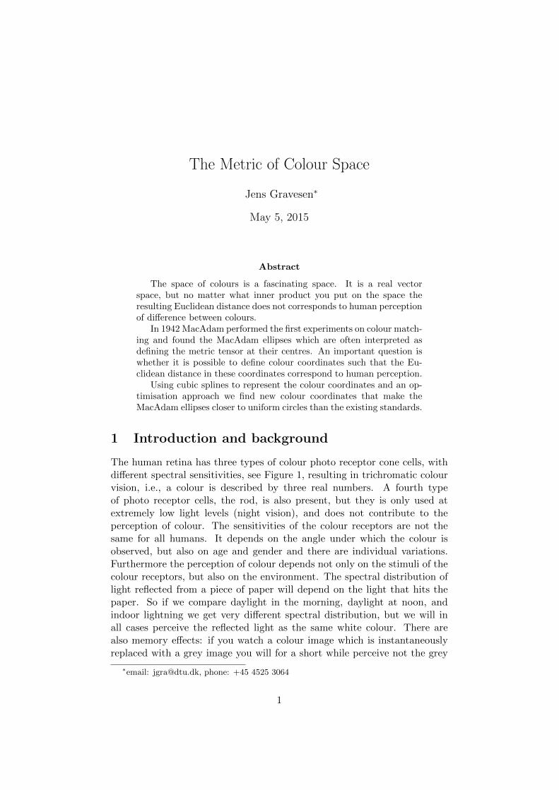
where ρ(λ) ∈ [0, 1] is the spectral reflectance of the object. The possiblecolour stimuli that can be obtained, when the incident light is some standardlight source such as D65, are convex combinations of optimal colour stimuli,i.e., light reflected from objects whose spectral reflectance ρ(λ) ∈ 0, 1 iseither constant zero except in an interval [λ1, λ2] where it is one, type 1,or vice verse for type 2, see Figure 3. The width of the interval [λ1, λ2]

wavelength λ/nm400 500 600 7000

0.5

1

λ1 λ2

wavelength λ/nm

400 500 600 7000

0.5

1

λ1 λ2

Figure 3: Spectral reluctance curves for the two types of optimal colourstimuli. Type 1 to the left and type 2 to the right.

is chosen such that luminance Y is some given value, normally given as apercentage of the luminance of the illuminant.

Ideally we would like the eye sensitivities (l,m, s) to be a linear combi-nation of (x, y, z), but this is not the case. Indeed, if we determine a 3 × 3matrix C in the least square sense such that (l,m, s)T = C (x, y, z)T , thenwe obtain l

ms

≈ 0.2684 0.8466 −0.0349−0.3869 1.1681 0.10310.0214 −0.0247 0.5388

xyz

, (4)

and, as we can see in Figure 4, we do not have a strict equality.

wavelength λ/nm400 500 600 700

0

0.2

0.4

0.6

0.8

1

wavelength λ/nm400 500 600 700

-0.1

0

0.1

0.2

Figure 4: To the left (l,m, s) in solid lines and C (x, y, z)T in dashed lines.To the right the difference.

The CIE xy chromatic coordinates are given by

x =X

X + Y + Z, y =

Y

X + Y + Z. (5)

5

Sometimes a third coordinate z = Z/(X+Y +Z) is defined, but it can alwaysbe found from the relation x+ y + z = 1. The two chromatic coordinates xand y describe “pure” colour, in the absence of luminance (or brightness).When monochromatic light sweeps over the visual light range from 400nm to700nm, it traces a curve in the xy-space, see Figure 5. The line connecting

x

0 0.2 0.4 0.6 0.8

y

0

0.2

0.4

0.6

0.8

400nm

475nm

500nm

525nm

550nm

575nm

600nm625nm

700nm

20

50

Figure 5: The tristimulus diagram. The monochromatic colours lie on thecurved part of the boundary. The dashed line joining the the end of thevisible spectrum [380nm, 700nm] is the line of purples. The triangle containthe colours that can be produced by the primaries of the Rec. 709 RGBspecifications (HDTV), [1]. The circle indicates the D65 white point and thetwo inner curves are the optimal colour stimuli for the D65 illuminant at20% and 50%, respectively.

the two ends of the curve is called the line of purples. It joins extreme bluewith extreme red and consists consequently of mixtures of blue and red.

A colour can be specified by chromaticity (x, y) and luminance Y inthe form of the CIE xyY components. To recover X and Z the followingformulae are used:

X = Yx

y, Z = Y

1− x− yy

. (6)

The colours on a computer screen or a television are given by mixing threeprimaries: red, green, and blue. The three primaries correspond to threepoints in xy-space and the screen can reproduce all colours in the trianglespanned by the three primaries, the gamut of the primaries. In Figure 5 theprimaries for the HDTV, [1], are plotted and it is easily seen that not allcolours can be obtained. The actual colours in the plot need not be correct,they depend on the computer screen, or on the printer and the illumination.Other devices such as a computer screen, a projector, etc. also have threeprimary colours and can only reproduce the colours in some triangle.

6

2.1 Uniform CIE colour spaces

The CIE Luv coordinates (1976), [12] is an attempt to create a perceptuallyuniform colour space and the components are given by

L∗ =

903.3Y/Yn if Y/Yn ≤ 0.008856 ,

116 3√Y/Yn − 16 if Y/Yn > 0.008856 ,

(7)

u∗ = 13L∗(u′ − u′n) , (8)

v∗ = 13L∗(v′ − v′n) . (9)

The quantities u′, v′, u′n, and v′n are given by

u′ =4X

X + 15Y + 3Z, u′n =

4Xn

Xn + 15Yn + 3Zn, (10)

v′ =9Y

X + 15Y + 3Z, v′n =

9YnX + 15Yn + 3Zn

. (11)

The triple (Xn, Yn, Zn) defines the origin in the u∗v∗-plane and consists ofthe components of the white reference, where Yn is normalised to 100. Forthe D65 white point the values are (Xn, Yn, Zn) = (95.043, 100, 108.88).

In the CIE Lab coordinates (1976) the components (u∗, v∗) are replacedby (a∗, b∗) that are given by

a∗ = 500(f(X/Xn)− f(Y/Yn)

), (12)

b∗ = 200(f(Y/Yn)− f(Z/Zn)

), (13)

where

f(t) =

7.787 t+ 16/116 if t ≤ 0.008856 ,3√t if t > 0.008856 .

(14)

In the CIE Lch coordinates the Cartesian coordinates (a∗, b∗) are replacedby polar coordinates (c, h) called chroma and hue respectively, i.e.,

a∗ = c cosh , b∗ = c sinh . (15)

3 Colour Differences

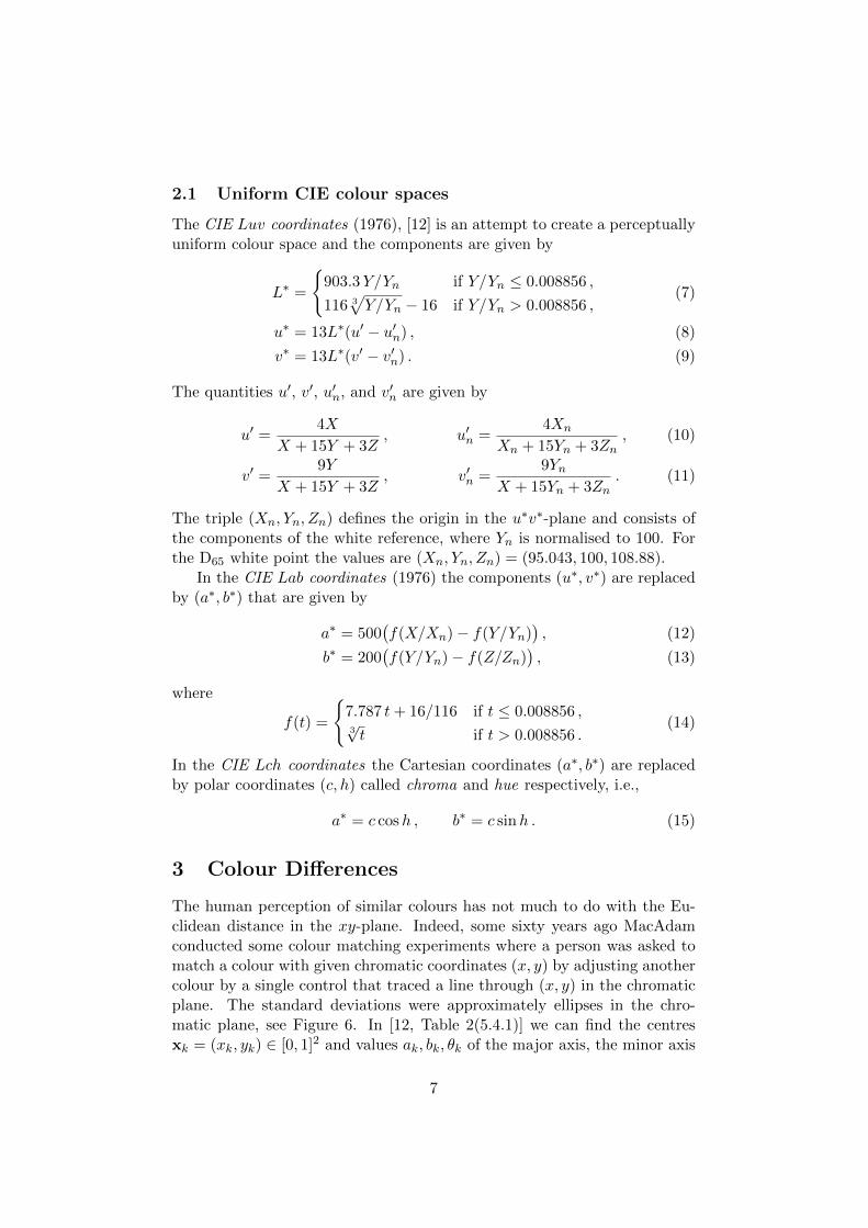
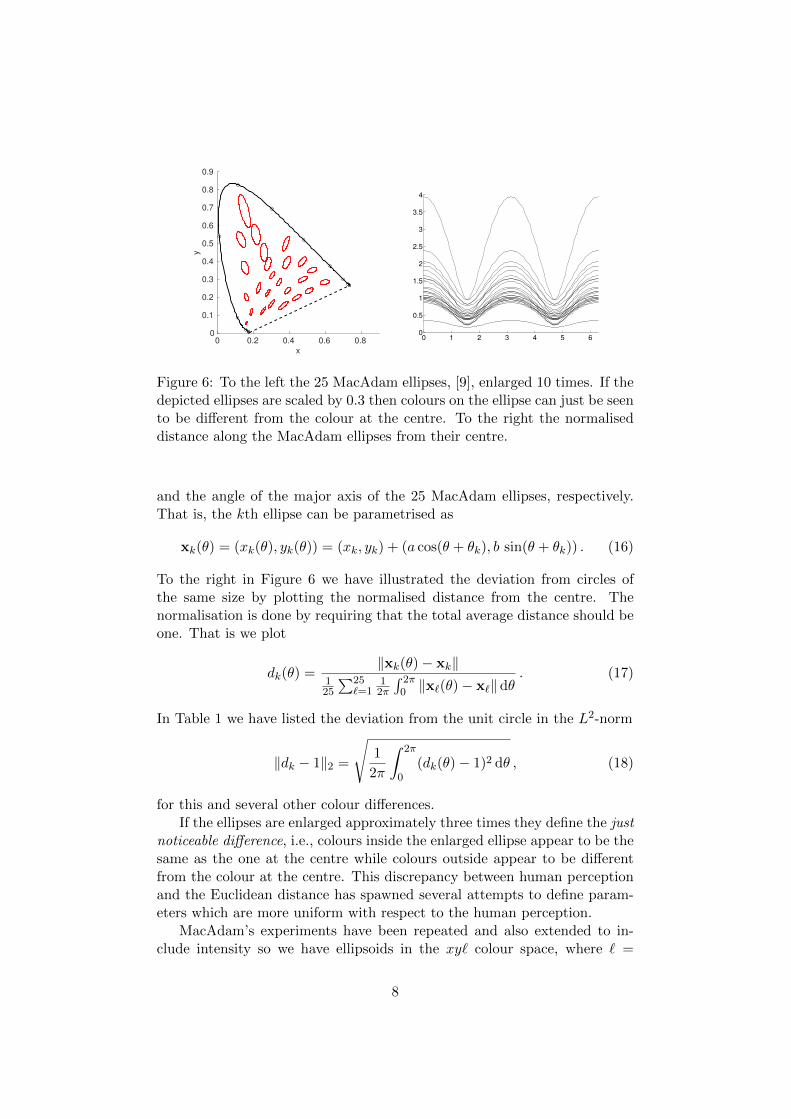
The human perception of similar colours has not much to do with the Eu-clidean distance in the xy-plane. Indeed, some sixty years ago MacAdamconducted some colour matching experiments where a person was asked tomatch a colour with given chromatic coordinates (x, y) by adjusting anothercolour by a single control that traced a line through (x, y) in the chromaticplane. The standard deviations were approximately ellipses in the chro-matic plane, see Figure 6. In [12, Table 2(5.4.1)] we can find the centresxk = (xk, yk) ∈ [0, 1]2 and values ak, bk, θk of the major axis, the minor axis

7

x

0 0.2 0.4 0.6 0.8

y

0

0.1

0.2

0.3

0.4

0.5

0.6

0.7

0.8

0.9

0 1 2 3 4 5 60

0.5

1

1.5

2

2.5

3

3.5

4

Figure 6: To the left the 25 MacAdam ellipses, [9], enlarged 10 times. If thedepicted ellipses are scaled by 0.3 then colours on the ellipse can just be seento be different from the colour at the centre. To the right the normaliseddistance along the MacAdam ellipses from their centre.

and the angle of the major axis of the 25 MacAdam ellipses, respectively.That is, the kth ellipse can be parametrised as

xk(θ) = (xk(θ), yk(θ)) = (xk, yk) + (a cos(θ + θk), b sin(θ + θk)) . (16)

To the right in Figure 6 we have illustrated the deviation from circles ofthe same size by plotting the normalised distance from the centre. Thenormalisation is done by requiring that the total average distance should beone. That is we plot

dk(θ) =‖xk(θ)− xk‖

125

∑25`=1

12π

∫ 2π0 ‖x`(θ)− x`‖ dθ

. (17)

In Table 1 we have listed the deviation from the unit circle in the L2-norm

‖dk − 1‖2 =

√1

2π

∫ 2π

0(dk(θ)− 1)2 dθ , (18)

for this and several other colour differences.If the ellipses are enlarged approximately three times they define the just

noticeable difference, i.e., colours inside the enlarged ellipse appear to be thesame as the one at the centre while colours outside appear to be differentfrom the colour at the centre. This discrepancy between human perceptionand the Euclidean distance has spawned several attempts to define param-eters which are more uniform with respect to the human perception.

MacAdam’s experiments have been repeated and also extended to in-clude intensity so we have ellipsoids in the xy` colour space, where ` =

8

0.2 log10(Y ), see [12, Tables I and II(5.4.2), and I(5.4.3–4)]. We don’t havethe 3D results in electronic form so all numerical experiments are done usingthe MacAdam ellipses in the 2D xy colour space.

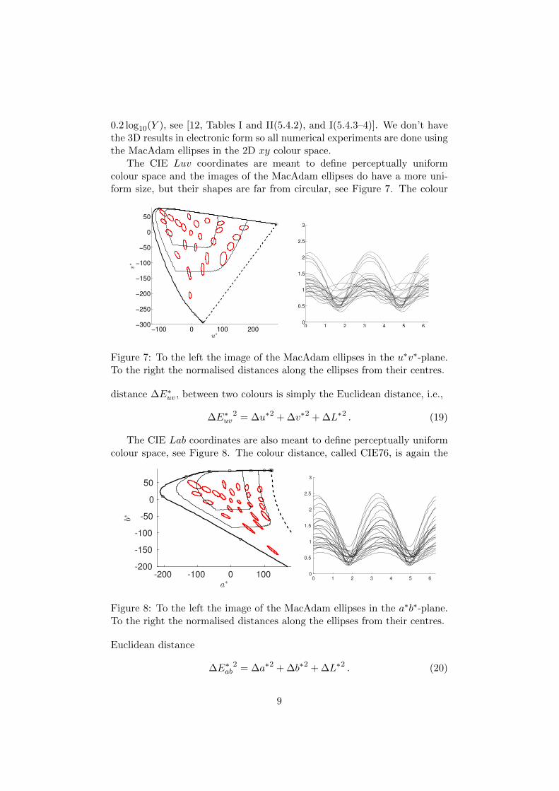
The CIE Luv coordinates are meant to define perceptually uniformcolour space and the images of the MacAdam ellipses do have a more uni-form size, but their shapes are far from circular, see Figure 7. The colour

−100 0 100 200−300

−250

−200

−150

−100

−50

0

50

u∗

v∗

0 1 2 3 4 5 60

0.5

1

1.5

2

2.5

3

Figure 7: To the left the image of the MacAdam ellipses in the u∗v∗-plane.To the right the normalised distances along the ellipses from their centres.

distance ∆E∗uv, between two colours is simply the Euclidean distance, i.e.,

∆E∗uv2 = ∆u∗2 + ∆v∗2 + ∆L∗2 . (19)

The CIE Lab coordinates are also meant to define perceptually uniformcolour space, see Figure 8. The colour distance, called CIE76, is again the

a∗

-200 -100 0 100

b∗

-200

-150

-100

-50

0

50

0 1 2 3 4 5 60

0.5

1

1.5

2

2.5

3

Figure 8: To the left the image of the MacAdam ellipses in the a∗b∗-plane.To the right the normalised distances along the ellipses from their centres.

Euclidean distance

∆E∗ab2 = ∆a∗2 + ∆b∗2 + ∆L∗2 . (20)

9

The CIE94 colour distance ∆Ech uses the polar coordinates croma and hue(15) and the distance between the colours (L∗1, c1, h1) and (L∗2, c2, h2) isdefined by

∆Ech2 =

(∆L∗

KL SL

)2

+

(∆c

Kc Sc

)2

+

(∆h

Kh Sh

)2

, (21)

where ∆h is defined such that

∆c2 + ∆h2 = ∆a∗2 + ∆b∗2 , (22)

i.e.,

∆Ech2 =

(∆L∗

KL SL

)2

+

(∆c

Kc Sc

)2

+∆a∗2 + ∆b∗2 −∆c2

(Kh Sh)2. (23)

The terms in the denominator depend on the application. In the case ofgraphic arts they are

SL = 1 , Sc = 1 + 0.045 c1 , Sh = 0.015 c1 , (24)

KL = 1 , Kc = 1 , Kh = 1 . (25)

Observe that the distance is asymmetric. In Figure 9 we have plotted the

0 2 4 60

0.5

1

1.5

2

2.5

3

0 2 4 60

1

2

3

4

5

6

0 2 4 60

0.5

1

1.5

2

2.5

3

3.5

4

Figure 9: To the left the CIE94 distance (normalised) along the ellipses fromtheir centres. In the centre and to the right, the same using the CMC 2:1distance and the CIEDE2000 distance, respectively.

distances along the ellipses from their centres according to this definition.The CMC l:c distance (1984) is also based on Lch coordinates and is givenas follows

∆E`:c2 =

(∆L∗

` SL

)2

+

(∆c

c Sc

)2

+∆a∗2 + ∆b∗2 −∆c2

(Sh)2, (26)

where ` = 2 and c = 1 are often used and

SL =

0.511 L∗1 < 16 ,0.040975L∗11+0.01765L∗

1L∗1 ≥ 16 ,

(27)

SC =0.0638 c1

1 + 0.0131 c1, (28)

Sh = SC (F T + 1− F ) , (29)

10

and

F =

√c41

1900 + c41, (30)

T =

0.56 + |0.2 cos(h1 + 168)| 164 ≤ h1 ≤ 345 ,

0.36 + |0.4 cos(h1 + 35)| otherwise.(31)

The result is plotted in Figure 9. Again we have an asymmetric distance.We finally look at the CIEDE2000 distance. It too is based on the Lchcolour space

∆E002 =

(∆L∗

kL SL

)2

+

(∆C ′

kC SC

)2

+

(∆H ′

kH SH

)2

+RT∆C ′

kC SC

∆H ′

kH SH, (32)

where

c =c1 + c2

2, (33)

a′i = a∗i +a∗i2

1−

√c7

c7 + 257

, (34)

(a′i, b∗i ) = C ′i(cosh′i, sinh

′i) , hi ∈ [0, 2π[ , (35)

C ′ =C ′1 + C ′2

2, (36)

∆h′ =

h′2 − h′1 , |h′2 − h′1| ≤ π ,h′2 − h′1 − 2π , h′2 − h′1 > π ,

h′2 − h′1 + 2π , h′2 − h′1 < −π ,(37)

∆H ′ = 2√C ′1C

′2 sin

(∆h′

2

), (38)

h′ =

(h′1 + h′2)/2 , |h′2 − h′1| ≤ π ,(h′1 + h′2 + 2π)/2 , |h′2 − h′1| > π , h′1 + h′2 < 2π ,

(h′1 + h′2 − 2π)/2 , |h′2 − h′1| > π , h′1 + h′2 ≥ 2π ,

(39)

T = 1− 0.17 cos(h′ − 30) + 0.24 cos(2h′)

+ 0.32 cos(3h′ + 6)− 0.20 cos(4h′ − 63) , (40)

L =L∗1 + L∗2

2, (41)

SL = 1 +0.015(L− 50)2√20 + (L− 50)2

, (42)

SC = 1 + 0.045C ′ , (43)

SH = 1 + 0.015C ′ T , (44)

11

RT = −2

√C ′

7

C ′7

+ 257sin

(60 exp

(−h′ − 275

25

)). (45)

The result is plotted in Figure 9.

4 New colour coordinates

We define the new coordinates in a two stage process where we first obtaina Riemannian metric on the colour space and then find a near isometry toEuclidean space.

4.1 Extrapolating the MacAdam Ellipses or the Metric

By regarding the MacAdam ellipses as being in the tangent space at thecentre xk we can identify them with a metric on the tangent space given by(

Ek FkFk Gk

)=

(cos θk − sin θksin θk cos θk

)(1/a2k 0

0 1/b2k

)(cos θk sin θk− sin θk cos θk

). (46)

We now extrapolate the components of this metric to the rectangle Ω =[0.0, 0, 8]×[0.0, 0.9]. In order to keep the matrix positive definite we considerthe matrix logarithm(

ek fkfk gk

)= log

(Ek FkFk Gk

)= −2

(cos θk − sin θksin θk cos θk

)(log ak 0

0 log bk

)(cos θk sin θk− sin θk cos θk

), (47)

We extrapolate the components to Ω by solving the following linear con-strained quadratic optimisation problem:

minimise

∫ 0.9

0

∫ 0.8

0

∣∣∣∣ ∂2e∂x2

∣∣∣∣2 + 2

∣∣∣∣ ∂2e∂x∂y

∣∣∣∣2 +

∣∣∣∣∂2e∂y2

∣∣∣∣2 dx dy , (48)

such that e(xk, yk) = ek, k = 1, . . . ,K , (49)

and similar for f and g. We use cubic B-splines to represent the functionse, f , and g and quadprog from Matlab’s Optimisation toolbox [10] to solvethe optimisation problem. We find the components of the metric by takingthe matrix exponential(

E(x, y) F (x, y)F (x, y) G(x, y)

)= exp

(e(x, y) f(x, y)f(x, y) g(x, y)

)(50)

the corresponding field of ellipses can be seen in Figure 10 together with theGaussian curvature. As we can see the Gaussian curvature is not zero so wecannot get a perfect isometry with Euclidean space.

12

0 0.2 0.4 0.60

0.2

0.4

0.6

0.8

0 0.2 0.4 0.60

0.2

0.4

0.6

0.8

0

0.005

0.01

0.015

0.02

0.025

0.03

0.035

Figure 10: To the left the black ellipses are the result of interpolating (andextrapolating) the metric corresponding to the MacAdam ellipses. Theknots are indicated by the thin lines. To the right the Gaussian curvature.

4.2 Obtaining a near isometry to Euclidean space

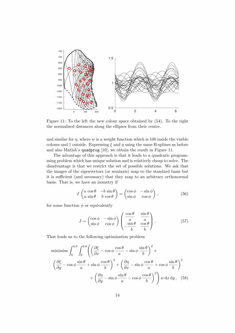
We seek a map (ξ, η) : Ω→ R2 such that the Euclidean distance in ξη spaceis in good agreement with human perception of colour distance. That is, wewant the images of the ellipses to be circles of equal size. This is the sameas saying that we have an isometry with respect to the extrapolated metricon Ω and the standard Euclidean metric on R2.

If the major and minor axes of the ellipses, or equivalently the eigenvec-tors of the metric tensor, map to the standard basis in R2 then we do havean isometry. The Jacobian of our map is

J =

(∂ξ/∂x ∂ξ/∂y∂η/∂x ∂η/∂y

), (51)

the eigenvectors are (a cos θ, a sin θ) and (−b sin θ, b cos θ), respectively, andthey map to the standard basis if

J

(a cos θ −b sin θa sin θ b cos θ

)=

(1 00 1

), (52)

or equivalently

J =

(a cos θ −b sin θa sin θ b cos θ

)−1=

1

ab

(b cos θ b sin θ−a sin θ a cos θ

). (53)

We now solve the quadratic optimisation problem

minimise

∫ 0.9

0

∫ 0.8

0

((∂ξ

∂x− cos θ

a

)2

+

(∂ξ

∂y− sin θ

a

)2)w dx dy (54)

such that ξ(0.1, 0.0) = 0 , (55)

13

0 100 200

-1200

-1150

-1100

-1050

-1000

-950

-900

-850

-800

-750

-700

0 2 4 60.5

1

1.5

Figure 11: To the left the new colour space obtained by (54). To the rightthe normalised distances along the ellipses from their centre.

and similar for η, where w is a weight function which is 100 inside the visiblecolours and 1 outside. Expressing ξ and η using the same B-splines as beforeand also Matlab’s quadprog [10], we obtain the result in Figure 11.

The advantage of this approach is that it leads to a quadratic program-ming problem which has unique solution and is relatively cheap to solve. Thedisadvantage is that we restrict the set of possible solutions. We ask thatthe images of the eigenvectors (or semiaxis) map to the standard basis butit is sufficient (and necessary) that they map to an arbitrary orthonormalbasis. That is, we have an isometry if

J

(a cos θ −b sin θa sin θ b cos θ

)=

(cosφ − sinφsinφ cosφ

), (56)

for some function φ or equivalently

J =

(cosφ − sinφsinφ cosφ

) cos θ

a

sin θ

a

−sin θ

b

cos θ

b

. (57)

That leads us to the following optimisation problem

minimise

∫ 0.9

0

∫ 0.8

0

((∂ξ

∂x− cosφ

cos θ

a− sinφ

sin θ

b

)2

+(∂ξ

∂y− cosφ

sin θ

a+ sinφ

cos θ

b

)2

+

(∂η

∂x− sinφ

cos θ

a+ cosφ

sin θ

b

)2

+

(∂η

∂y− sinφ

sin θ

a− cosφ

cos θ

b

)2)w dx dy , (58)

14

such that (ξ(0.1, 0), η(0.1, 0)) = (0, 0) and φ(0.1, 0) = 0. This is not aquadratic problem and we now use Matlab’s fmincon [10] to solve the opti-misation problem. The result is shown in Figure 12.

150 200 250 300 350 400 450

-50

0

50

100

150

200

250

300

350

400

0 2 4 60.5

1

1.5

Figure 12: To the left the new colour space obtained by (58). To the rightthe normalised distances along the ellipses from their centre.

A warning is wareanted here. There is nothing that guaranties that theoptimisations (54) and (58) give an injective map (ξ, η) : Ω→ R2. Indeed ifwe use a coarse spline space then (58) yields a non injective map. This canbe circumvented by adding det J > 0 as a constraint in the optimisation.Here it is crucial to express det J in B-spline form, see [7, Theorem 1].

It should also be noted that we have assumed that the axes of theMacAdam ellipses (a cos θ, a sin θ) form a smooth vector field, i.e., we chosethe eigenvectors of the metric (50) such that they form smooth vector fields.This can always be done, but could be cumbersome. Alternatively we coulduse that our map is an isometry if and only if

JTJ =

(ξ2x + η2x ξx ξy + ηx ηy

ξx ξy + ηx ηy ξ2y + η2y

)=

(E FF G

), (59)

where ξx, ξy, ηx, and ηy denotes the partial derivatives. This would give usthe following optimisation problem

minimise

∫ 0.9

0

∫ 0.8

0

(ξ2x + η2x − E

)2+ 2 (ξx ξy + ηx ηy − F )2

+(ξ2x + η2x −G

)2dx dy . (60)

5 Results

The results are summarised in Table 1 where we have listed how much the

15

i xy uv ab CIE94 CMC CIE00 new 1 new 2

1 7.49 3.61 7.81 5.47 4.82 5.23 0.58 0.372 4.48 6.83 9.47 4.30 4.05 4.09 0.72 1.153 4.18 6.32 7.20 3.89 4.17 3.66 2.65 1.024 19.84 3.20 8.76 1.33 2.64 3.19 1.14 0.915 5.86 2.56 4.43 2.84 3.98 3.31 1.07 0.436 9.03 2.12 3.17 0.86 2.73 3.14 0.99 1.657 6.68 2.43 2.92 2.72 1.72 4.92 0.81 1.398 3.44 2.15 4.29 3.06 2.87 3.62 1.02 0.999 4.07 2.20 2.63 5.27 3.75 5.61 1.78 0.91

10 5.18 3.34 3.55 2.41 2.83 2.78 1.47 2.5111 3.89 2.95 3.93 9.14 6.41 7.40 1.40 0.8312 3.32 3.62 3.30 8.00 7.78 4.59 0.96 0.9613 3.70 3.78 4.92 5.09 31.52 8.66 1.60 0.7214 3.54 1.58 2.56 6.68 8.60 11.51 1.47 1.7615 2.60 2.19 2.79 4.04 7.42 6.68 1.32 1.5416 2.58 2.32 2.96 2.62 2.93 3.85 1.84 0.3617 2.91 1.69 3.38 3.02 3.31 3.87 1.97 0.5418 2.96 1.25 2.85 3.64 4.89 4.21 0.70 0.6119 2.58 3.31 1.97 3.18 3.89 3.89 0.35 0.3020 3.70 2.97 4.33 2.78 2.69 2.74 1.13 0.3821 3.28 1.41 3.38 3.02 4.14 3.18 0.67 0.7322 3.20 1.96 2.75 3.62 4.92 3.99 1.16 1.0623 4.21 3.34 4.14 3.19 3.99 2.84 2.00 1.8924 3.78 5.63 5.14 3.53 4.14 3.53 2.50 1.4525 3.75 7.55 6.15 3.08 3.67 3.25 1.82 0.66

avg 4.81 3.21 4.35 3.87 5.35 4.55 1.32 1.00

Table 1: The deviation of the MacAdam’s ellipses from the unit circle mea-sured in the L2 norm, cf. (18). The worst cases are marked with a greybackground.

MacAdam’s ellipses deviate from the unit circle in the L2-norm, see (17)and(18), for all the colour differences considered in this paper. As we havedefined the distance from the centre of the ellipses to any point on theellipse to be one it is clearly seen that the Euclidean distance in two newcolour spaces are significantly closer to MacAdam’s observations than anyof the classical colour distances.

6 Mathematical afterthoughts

In the preceding sections we have identified the MacAdam ellipses witha metric on the tangent space at the centre of the ellipses. This is an

16

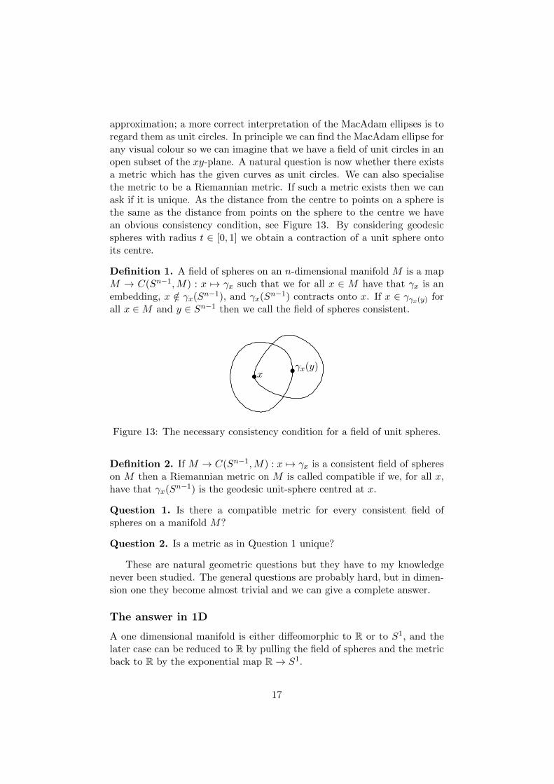
approximation; a more correct interpretation of the MacAdam ellipses is toregard them as unit circles. In principle we can find the MacAdam ellipse forany visual colour so we can imagine that we have a field of unit circles in anopen subset of the xy-plane. A natural question is now whether there existsa metric which has the given curves as unit circles. We can also specialisethe metric to be a Riemannian metric. If such a metric exists then we canask if it is unique. As the distance from the centre to points on a sphere isthe same as the distance from points on the sphere to the centre we havean obvious consistency condition, see Figure 13. By considering geodesicspheres with radius t ∈ [0, 1] we obtain a contraction of a unit sphere ontoits centre.

Definition 1. A field of spheres on an n-dimensional manifold M is a mapM → C(Sn−1,M) : x 7→ γx such that we for all x ∈ M have that γx is anembedding, x /∈ γx(Sn−1), and γx(Sn−1) contracts onto x. If x ∈ γγx(y) forall x ∈M and y ∈ Sn−1 then we call the field of spheres consistent.

xγx(y)

Figure 13: The necessary consistency condition for a field of unit spheres.

Definition 2. If M → C(Sn−1,M) : x 7→ γx is a consistent field of sphereson M then a Riemannian metric on M is called compatible if we, for all x,have that γx(Sn−1) is the geodesic unit-sphere centred at x.

Question 1. Is there a compatible metric for every consistent field ofspheres on a manifold M?

Question 2. Is a metric as in Question 1 unique?

These are natural geometric questions but they have to my knowledgenever been studied. The general questions are probably hard, but in dimen-sion one they become almost trivial and we can give a complete answer.

The answer in 1D

A one dimensional manifold is either diffeomorphic to R or to S1, and thelater case can be reduced to R by pulling the field of spheres and the metricback to R by the exponential map R→ S1.

17

A field of spheres on R is simply two maps a, b : R → R, such thata(x) < x < b(x), for all x ∈ R. The consistency condition reads

x ∈ a(a(x)), b(a(x)) , and x ∈ a(b(x)), b(b(x)) . (61)

As a(a(x)) < a(x) < x < b(x) < b(b(x)) we must have x = b(a(x)) andx = a(b(x)), i.e.,

a = b−1 , and hence a′(b(s)) b′(s) = 1 . (62)

A Riemannian metric on R is simply a weight function α : R → R+ anda(x), b(x) is a unit sphere centred at x if and only if∫ x

a(x)α(t) dt = 1 , and

∫ b(x)

xα(t) dt = 1 . (63)

Differentiation with respect to x yields

a′(x)α(a(x)) = α(x) , and b′(x)α(b(x)) = α(x) . (64)

Now assume that a, b are C1-functions such that a(x) < x < b(x) anda = b−1. Let α : [0, b(0)]→ R+ be a positive function such that∫ b(0)

0α(t) dt = 1 . (65)

we extend α to [a(0), 0[ by letting α(x) = α(b(x)) b′(x) and to ]b(0), b(b(0))]by letting α(x) = α(a(x)) a′(x). Repeating this procedure we extend α to amap R→ R+. For x ∈ [0, b(0)] we now have∫ b(x)

xα(t) dt =

∫ b(0)

xα(t) dt+

∫ b(x)

b(0)α(t) dt

substituting t = b(s) in the second integral yields

=

∫ b(0)

xα(t) dt+

∫ x

0α(b(s)) b′(s) ds

=

∫ b(0)

xα(t) dt+

∫ x

0α(a(b(s))) a′(b(s)) b′(s) ds

=

∫ b(0)

xα(t) dt+

∫ x

0α(s) ds = 1 .

Similarly we see that∫ xa(x) α(t) dt = 1 and that it also holds for x ∈ [a(0), 0[

and more generally for x ∈ [an(0), an−1(0)[ and x ∈]bn−1(0), bn(0)], i.e., forall x ∈ R. So in the one dimensional case we have a solution but it is farfrom unique, any function α : [0, b(0)]→ R+ satisfying (65) gives a solution.

18

7 Conclusion and future work

We have presented a two stage process that provides us with new colourcoordinates. As seen in Table 1 the Euclidean distance in these new colourspaces reflects human perception better than the existing standards. Thenew coordinates are given in terms of B-splines so evaluation of them arevery fast.

Viewing the MacAdam ellipses as unit circles leads to a new and so farunstudied geometrical problem, where we can give the full answer in thesimple one dimensional case.

The present work is certainly not the end of the story. I am convincedthat step one in the algorithm, determing the Riemannian metric, can beimproved and the different approaches mentioned in Section 1 should betried. The construction should be carried out in the full 3D colour spacetaking all available data into account. Ideally the resulting colour differencesshould be validated by performing new experiments.

References

[1] ITU-R Recommendation BT. 709. Basic Parameter Values for theHDTV Standard for the Studio and for the International Program Ex-change. ITU, 1211 Geneva 20, Switzerland, 1991.

[2] CIE colour matching functions. http://cvrl.ioo.ucl.ac.uk/cmfs.

htm.

[3] CIE 116:1995 industrial colour-difference evaluation. Technical report,CIE, 1995.

[4] CIE 142:2001 Improvement to industrial colour-difference evaluation.Technical report, CIE, 2001.

[5] CIE 170-1:2006 Fundamental chromaticity diagram with physiologicalaxes - part 1. Technical report, CIE, 2006. ISBN: 978 3 901906 46 6.

[6] H.J.A. Dartnell, J.K. Bowmaker, and J.D. Mollon. Human visual pig-ments: Microspectrophotometric results from the eyes of seven persons.Proc. Royal Soc. London. Series B, Biological Sciences, 220:115–130,1983.

[7] J. Gravesen, A. Evgrafov, D.M. Nguyen, and P. Nørtoft. Planarparametrization in isogeometric analysis. In M. Floater, T. Lyche, M.-L. Mazure, K. Mørken, and L. Schumaker, editors, Proceedings of the”Eighth International Conference on Mathematical Methods for Curvesand Surfaces. Oslo, 2012, volume 8177 of Lecture Notes in ComputerScience, pages 189–212. Springer, 2014.

19

[8] I. Lissner and P. Urban. Toward a unified color space for perception-based image processing. IEEE Transaction on Image Processing,21:1153–1168, 2012.

[9] D. L. MacAdam. Visual sensitivities to color differences in daylight. J.Optical Soc. Amer., 32:247–274, 1942.

[10] MathWorks, Natick, Ma. Matlab R2014b. Optimization Toolbox. User’sGuide, 2014.

[11] G. Sharma, W. Wu, and E.N. Dalai. The ciede2000 color-differenceformula: Implementation notes, supplementary test data, and mathe-matical observations. Color Research & Applications, 30:21–30, 2004.

[12] Gunter Wyszecki and W. S. Stiles. Color Science, Concepts and Meth-ods, Quantitative Data and Formulae. John Wiley & Sons, New York,Chichester, Brisbane, Toronto, Singapore, 2. edition, 1982.

20