Embed Size (px)
Citation preview

1
The New Meteorological Research Institute Coupled GCM (MRI-CGCM2) --- Model Climate and Variability ---
by
Seiji Yukimoto, Akira Noda, Akio Kitoh, Masato Sugi, Yoshiteru Kitamura, Masahiro Hosaka,
Kiyotaka Shibata, Shuhei Maeda and Takao Uchiyama
Papers in Meteorology and Geophysics Vol. 51, No. 2, pp. 47-88, February 2001
Meteorological Research Institute, Tsuikuba, Ibaraki, 305-0052, Japan

2
Abstract
A new version of a global coupled atmosphere-ocean general circulation model (MRI-CGCM2) has been developed at the Meteorological Research Institute (MRI). The model can be used to explore climate change associated with anthropogenic forcings. We aimed to reduce the drawbacks of the former version of the model (MRI-CGCM1, Tokioka et al., 1996) and achieve a more realistic climatic mean and variability to predict climate changes with greater accuracy.
In a preliminary analysis of the control run, the model showed generally good performance in reproducing the mean climate (including seasonal variation) in representative aspects; surface air temperature, precipitation, snow and sea ice distribution, and ocean structure and circulation. The model is capable of making a stable integration longer than 200 years. The sea ice distribution is much improved and is close to the observed extent and thickness. The model simulates realistic strength of meridional overturning in the Atlantic Ocean that MRI-CGCM1 failed to simulate. The model realistically simulates variabilities such as Arctic Oscillation (AO) and ENSO.
Temporal variation of the sea surface temperature (SST) anomaly in the NINO3 region (150°W to 90°W, 4°S to 4°N) shows a large positive value (max. +4°C) with several years interval. The SST anomaly pattern is similar to the observed El Niño with a strong positive anomaly in the central-eastern equatorial Pacific. The model still has some biases at present. The surface air temperature in winter at high latitude has a warm bias due to weaker stability in the boundary layer. The surface temperature over land in summer also shows a warm bias associated with a problem concerning the hydrological process.
1. Introduction
The new version of the global coupled atmosphere-ocean general circulation model (MRI-CGCM2), developed at the Meteorological Research Institute (MRI), is intended to enable examination of transient future climate changes associated with anthropogenic forcings such as the increase of greenhouse gases and sulfate aerosols. It is important for a climate model to be able to reproduce the present climate system realistically, including individual physical process components and interactions between them. For simulating the transient response of the climate system to specific influences, such as the IPCC scenario of an increase in greenhouse gases and aerosols, it is necessary for the model to simulate adequately not only the mean climate but also its variability.
At MRI, a series of experiments on global warming prediction was performed with a former climate model (MRI-CGCM1, Tokioka et al., 1996). The model simulated an increase in global mean surface air temperature of 1.6°C in 70 years in the experiment with atmospheric CO2 increasing by 1% per year compound. The result was comparable with an average of
results from other institutes (IPCC, 1996). The MRI-CGCM1 showed fairly good performance in reproducing interannual and interdecadal variability in the Pacific (Yukimoto et al., 1996). The magnitude of the equatorial SST anomaly was comparable to that in the observed El Niño and Southern Oscillation (ENSO). The model simulated realistic atmosphere-ocean interactions such as the westerly wind anomaly in the west-central equatorial Pacific in a warm phase, the eastward propagation of downwelling Kelvin waves, the equatorial thermocline deeper in the eastern and shallower in the western Pacific, and the westward propagation of Rossby waves off the equator. Moreover, MRI-CGCM1 simulated the interdecadal variability in the Pacific, which is similar to the observed decadal climate shift in the Pacific in 1976/77 (e.g., Nitta and Yamada, 1989), and showed realistic spatial and temporal structure of the variability in the Pacific throughout interannual to interdecadal time scales (Yukimoto et al., 2000). MRI-CGCM1 performed well in simulating the Asian summer monsoon as well as ENSO. The ENSO-monsoon relationship in the interannual variability is consistent with observation, where a good monsoon is associated with La Niña (Kitoh et al., 1999).

3
Using this strength, changes in the Asian summer monsoon in the global warming experiment were investigated (Kitoh et al., 1997).
Although the MRI-CGCM1 showed a fairly good performance in many aspects, it had several serious drawbacks. Firstly, the model showed a large climatological drift, which made it difficult to run beyond 150 years. Secondly, the thermohaline circulation in the Atlantic Ocean was not present in the model. Associated with this defect, there was no simulation of an increase minimum of surface temperature in the North Atlantic with the CO2 increase experiment, while an increase minimum is seen in results from many other models. The third problem was poor representation of sea ice. For the Norwegian Sea, the model simulated unrealistic sea ice cover that is not observed, resulting in a spurious large temperature increase by melting in the CO2 increase experiment. The Antarctic sea ice showed a trend of gradual decrease even in the control run, which caused difficulties in interpreting the Antarctic sea ice change in the warmer climate with the model experiment. The fourth problem was associated with the ENSO simulation, in which MRI-CGCM1 showed the equatorial SST anomaly maximum west of the date line. This location is further westward than observed.
In developing MRI-CGCM2, we aimed at eliminating the above drawbacks and achieving a better performance in reproducing the mean climate and the climate variability than MRI-CGCM1.
This paper is organized as follows: Section 2 describes the model and experimental design for the control run. Section 3 describes the model climatology of the control run. A preliminary analysis of the climate variability in the control run is presented in section 4. The summary and discussion are presented in section 5.
2. Modeling and Experiment Design
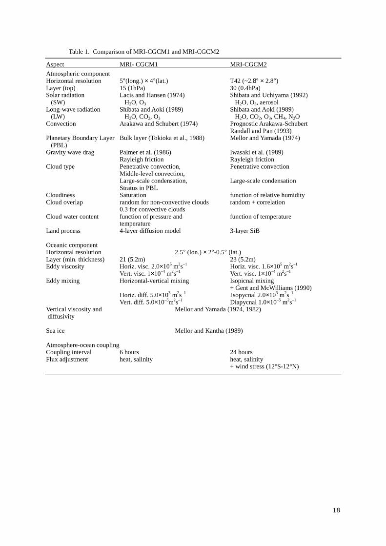
The model consists of an atmospheric general circulation model (AGCM) coupled with an oceanic general circulation model (OGCM). The AGCM includes a land process model and the OGCM includes a sea ice model. The differences between MRI-CGCM1 and MRI-CGCM2 are summarized in Table 1.
2.1 Atmospheric Model
The atmospheric component of the model is an early version of a new spectral AGCM (MRI/JMA98). This AGCM has been developed based on a version of the operational weather forecasting model of the Japan Meteorological Agency (JMA). Some physical process schemes are replaced with those of the original JMA version. Details of the AGCM are described in Shibata et al. (1999), so we give only an outline here.
The dynamic framework is completely replaced with a spectral transform method, while the AGCM in MRI-CGCM1 was a grid model (5° × 4°, 15 levels). The horizontal resolution is T42 in wave truncation and 128 × 64 in a transformed Gaussian grid (grid spacing approximately 2.8° × 2.8° in longitude and latitude). The vertical configuration consists of a 30-layer sigma-pressure hybrid coordinate with the top at 0.4hPa.
As in MRI-CGCM1, a multi-parameter random model based on Shibata and Aoki (1989) is used for terrestrial radiation. In the present version, absorption due to CH4 and N2O is treated in addition to H2O, CO2 and O3. The model calculates solar radiation formulated by Shibata and Uchiyama (1992) with delta-two-stream approximation. An explicit treatment of the direct effect of sulfate aerosols is possible in this scheme. The optical properties (diffusivity, single scattering albedo and asymmetry parameters) of sulfate aerosol are substituted by those for the LOWTRAN rural aerosol, which is composed of a mixture of 70% water soluble substance (ammonium and calcium sulfate and organic compounds) and 30% dust-like particles. Since complex refractive indices for water soluble and dust-like aerosols are very similar, particularly in the solar wavelength region, and can be regarded as identical in a first-order approximation, those parameters are applicable for sulfate aerosols as a whole. The effects of relative humidity on solution concentration and radius distribution of aerosols are incorporated.
For deep moist convection, the Arakawa-Schubert scheme with prognostic closure similar to Randall and Pan (1993) is used. For other physical parameterizations, mid-level convection that is moist convection rooted in a free atmosphere, large-scale condensation, vertical diffusion with a

4
level-2 turbulence closure scheme based on Mellor and Yamada (1974), orographic gravity wave drag scheme developed by Iwasaki et al. (1989) and Reyleigh friction as a non-orographic gravity wave drag are used.
2.2 Land Hydrology
Parameterization for ground hydrology of MRI-CGCM2 is based on the Simple Biosphere (SiB) model (Sellers et al., 1986; Sato et al., 1989) that treats effects of vegetation. No vegetation scheme was included in MRI-CGCM1. The model has three soil layers with a different field capacity for each vegetation type, where temperature, liquid water and frozen water in the soil layers are predicted. The scheme is improved from the older version to strictly preserve the budget of heat and water in the phase transition (melting and freezing) of soil water. This is an important matter for evaluating changes of snow cover and permafrost in global warming.
Runoff from the soil layers (surface runoff plus underground runoff) is transferred to either a river mouth grid or an inland waters grid through river routings specified by the terrain. In the present version, the flow rate parameter is set to move all the water storage in a grid box to the next downstream grid in one time-step. Therefore, practically, all the runoff is discharged immediately (within one day at most) at the river mouth. When accumulated snow over the ice-sheets of Antarctica and Greenland exceeded 10m of water-equivalent depth, the excess water is treated as runoff and discharged immediately to the ocean in the same manner as river runoff.
Inland waters are treated as terminal grid box(es) with a drainage basin unconnected to any ocean. The Caspian Sea, the Aral Sea, Lake Balkhash, Lake Chad and Lake Eyre (Australia) come under inland waters in the model. Fractional coverage of inland water in a grid box is considered. Storage of inland water changes by a balance between river discharge and precipitation and evaporation over the water area. Water temperature is predicted by the heat budget at the water surface, assuming a 50m-thick slab (independent of water storage).
2.3 Ocean Model The oceanic component of the model is
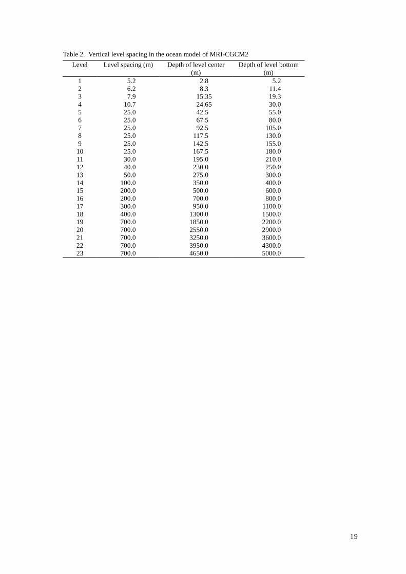
a Bryan-Cox type ocean general circulation model (OGCM) with a global domain, and its basic dynamic configuration is the same as in MRI-CGCM1. The horizontal grid spacing is 2.5 degrees in longitude and 2 degrees in latitude poleward of 12 degrees in both hemispheres. Near the equator, between 4°S and 4°N, the meridional grid spacing is set 0.5 degrees in order to provide good resolution of equatorial oceanic waves. The grid spacing gradually increases from 0.5 degrees to 2 degrees for latitudes of 4 to 12 degrees. The vertical level spacing is given in Table 2. The uppermost layer has 5.2 m thickness and the deepest bottom is set to 5000 m. There are two more levels for the upper thermocline than in MRI-CGCM1, aiming at a better representation of oceanic waves that play an important role in decadal to interdecadal climate variability.
The Denmark Strait is made slightly deeper and broader than the real topography to represent sub-grid scale overflow of waters formed in the Nordic Seas. This modification contributes somewhat to the improvement of thermohaline circulation in the North Atlantic, which will be shown later.
Parameterized sub-grid mixing processes using viscosities and diffusivities are specified as follows: the horizontal viscosity coefficient is 1.6 × 10⁵ m2s–1 and the vertical viscosity coefficient is 1 × 10⁻⁴ m2s–1. A new feature of the OGCM is the introduction of eddy mixing parameterization based on Gent and McWilliams (1990). Its isopycnal mixing coefficient is 2 × 10³ m2s–1 and diapycnal mixing coefficient is 1×10⁻⁵ m2s–1. The horizontal and vertical diffusivity coefficients of MRI-CGCM1were 2.5 times and five times larger than the isopycnal and diapycnal coefficients of MRI-CGCM2. With these diffusivity coefficients, the temperature gradient across the oceanic fronts becomes sharper, leading to stronger oceanic circulations and meridional overturnings than in MRI-CGCM1. To simulate the surface mixed layer, vertical turbulence viscosity and diffusivity following Mellor and Yamada (1974, 1982) and Mellor and Durbin (1975) are modeled in addition to isopycnal mixing. When vertical stratification becomes unstable, a convective adjustment is applied by mixing the whole

5
vertical column. Solar radiation penetrating seawater is absorbed with an e-folding of 10m-depth , heating the surface seawater to several dozenmeters.
2.4 Sea Ice Model
The sea ice model is basically the same as in MRI-CGCM1, that is, similar to the model by Mellor and Kantha (1989). Compactness and thickness are predicted based on thermodynamics and advection. The freezing (melting) rate of sea ice is calculated with balances of heat and freshwater at the sea ice bottom, the open sea surface and within seawater (creation of frazil ice).
Compactness is calculated using empirical constants (these are tuning parameters). The sea ice is advected by the surface ocean current multiplied by an empirical constant (set to 1/3 at present). Compactness is also advected by the surface ocean current, though it is limited to a maximum value of 0.997 in the Northern Hemisphere (NH) and to 0.98 in the Southern Hemisphere (SH). If the sea ice becomes very thick, gaps in sea ice (leads) are difficult to be filled by freezing at the sea surface, which results in the unlimittedincrease of sea ice by freezing at leads. In order to avoid this problem, we set compactness to the maximum values quoted above for sea ice thicker than 3 m for the NH and 1 m for the SH.
2.5 Coupling Scheme
The atmosphere and the ocean interact with each other by exchanging fluxes of heat, freshwater and momentum at the sea surface. The contents of the fluxes are sensible and latent heat fluxes, and net short-wave and long-wave radiation, precipitation and evaporation, river discharge and meltwater from snow and ice over sea ice, and zonal and meridional components of the surface wind stress. The fluxes are exchanged every 24 hours in the model. The AGCM (including land model) is time integrated for 24 hours and outputs averaged fluxes at the sea surface. The fluxes are transferred to the OGCM grid, with budgets maintained. The OGCM (including sea ice model) is then time integrated for 24 hours, and outputs the resulting SST and sea ice compactness and thickness for updating the lower boundary
for the AGCM. These procedures are repeated.
Since the grid boundary of the AGCM does not match that of the OGCM, the AGCM calculates fluxes independently for three surface conditions (land, sea and sea ice), considering fractional coverage in a single grid box. The AGCM treats averaged flux with area weighting as a flux at the atmosphere bottom. In this coupling process, heat and freshwater are transferred, preserving rigorous budgets.
2.6 Spin-up and Flux Adjustment
Arriving at a quasi-equilibrium state of coupled atmosphere and ocean as an initial condition for experiments with a coupled model is a difficult and important problem. The time scale of the ocean response to forcing ranges from several years to several decades even for the upper ocean, (depending, for example, on the latitudes of the variation), and more than a thousand years for the deep ocean. Therefore, the coupled model generally needs long-term spin-up, though it depends on the objective time scale of the experiment. We made a spin-up of the model, preparing for 200-year climate change experiments as shown in Table. 3.
As the response time of the ocean is much longer than that of the atmosphere, we made a spin-up of the ocean with an asynchronously coupled run (SPIN-UPs 1–5, 209-year) in order to save computational time. We ran the OGCM and the AGCM by turns of different length. A synchronously coupled spin-up of a further 111 years was then applied (SPIN-Ups 6-8). The forcing data and the boundary conditions vary at each stage of the spin-up as shown in Table.3, because we tried to avoid any abrupt shock to the coupled system from changing numerous conditions simultaneously.
In order to keep the model climatology of the control run close to the observed one, we used flux adjustments for heat and freshwater obtained from the spin-up run. Figure 1 shows geographical distribution of annual mean fluxes for heat and freshwater together with those in MRI-CGCM1 for comparison. The flux adjustments for heat and freshwater in the new model are generally smaller than in MRI-CGCM1. Major features of the adjustments, such as heating in the equatorial Pacific and cooling around Japan and Newfoundland, are

6
common to both models, in spite of completely different AGCMs. It is supposed that these large heat adjustments arise from insufficient representation of small-scale ocean dynamic effects such as equatorial waves, western boundary currents and coastal upwelling. Most other regions (where effects of such ocean dynamics are small) show smaller adjustments of less than 25 Wm–2 in MRI-CGCM2, whereas a relatively large proportion of regions have adjustments greater than 25 Wm–2 in MRI-CGCM1. Cooling in most coastal regions is notable in the new model. This is related to the lack of clouds, because the spectral atmospheric model cannot represent as sharp a land-sea humidity contrast as a grid model. The freshwater flux adjustment is generally large at river mouth points. In the Arctic Sea, there are large, patchy adjustment regions both positive and negative in value. Most other regions show relatively smaller adjustments of less than 5 mm/day. Compared to the former model, the negative freshening (salting) adjustment in the Norwegian Sea is much smaller. It is considered that the stronger North Atlantic thermohaline circulation contributes to the reduction of the freshwater adjustment.
Figure 2 shows the meridional distribution of the zonal mean fluxes and flux adjustments for heat and freshwater, for December to February (DJF) and June to August (JJA),. Fluxes based on observational estimation are also shown for comparison. The observational heat flux is from Da Silva et al. (1994), and the observational freshwater flux is the evaporation by Da Silva et al. (1994), subtracting the precipitation by Xie and Arkin (1996). Observational data are poor poleward of 45°S and 60°N.
The model’s heat fluxes agree with observations in most latitudes, though there is overestimation of heating in summer at latitudes higher than 30 degrees in both hemispheres. Some of these biases are compensated for by the flux adjustment.
However, at some latitudes (e.g. near the equator), the adjusted flux shows a larger bias than the original flux. The flux adjustments try to compensate for biases of the oceanic transports, as well as for biases of the atmospheric fluxes. For example, the strong heating adjustment near the equator implies compensation for cooling by too strong equatorial upwelling.
The freshwater fluxes agree with the observational estimation except for the equatorial region and the midlatitudes in boreal winter. However, large freshwater adjustments are seen, especially in the high latitudes. It is difficult for coupled models to successfully simulate the observed salinity distribution, since there is no explicit damping effect by the atmosphere on salinity anomalies, unlike with temperature.
We adjusted for wind stress only in the equatorial region to accurately represent the climatological thermocline structure along the equator, which plays a crucial role in model performance when simulating ENSO. On the equator (4°S to 4°N), the differences of climatology between the model and the observation (Hellerman and Rosenstein, 1983) are added to the model’s wind stress. A nine-point smoothing in zonal direction is applied to the adjustments. Off the equator (12°S to 4°S, 4°N to 12°N), the adjustment decreases with latitude and is set to zero poleward of 12°S and 12°N. The climatological wind stresses (zonal and meridional components) together with their adjustments for January and July are shown in Fig. 3. The adjustment of the zonal component is small except in the western Indian Ocean (January and July) and the western Pacific (July). The meridional component is generally enhanced by the adjustment, particularly in the eastern Pacific and the eastern Atlantic (January and July).
3. Climate of the Control Run
We made a 200-year control run of the model. This run is used as a reference for experimental projections of global warming. Concentrations of the greenhouse gases are
set constant at 348ppmv for CO2, 1.650 ppmv for CH4 and 0.306 ppmv for N2O. The seasonally varying ozone profile is prescribed to climatological data taken from Wang et al. (1995).
The climate of the three-dimensional structure of the simulated atmosphere is similar to that of the L30 version of MRI/JMA98 by Shibata et al. (1999). There

7
are many changes in the AGCM from the MRI-CGCM1. It is difficult to interpret the differences of the model results because many processes with different schemes are interacting in the simulations. The former AGCM was used for many climate studies and was well tuned as a climate model during its long history, showing good performance in various climatic aspects. Since the new AGCM is in the early stages of development as a climate model, there are many problems that should be evaluated and resolved in future studies. In the present paper, we focus on the climate of near surface fields that directly affect the ocean and the coupled system.
We use the NCEP/NCAR reanalysis (Kalney et al., 1996) climatology of 1979 to 1995 as the reference climatology for the atmospheric fields in the model evaluation. The reanalysis data are convenient, sufficiently reliable to compare the overall performance of the model, and reflect most available observational data. We refer to the reanalysis climatology as NRA hereafter.
We recognize that the period of the observational data is much shorter than that of the model run. It may not be statistically appropriate to compare datasets with these different sampling periods, since both the observation and the model run contain interdecadal variations as shown later. We tested the model evaluation with different 30-year averages and confirmed that the interdecadal variations do not affect the essential features of the differences between observation and model. We used the last 30-year average of the 200-year run as the model climatology.
3.1 Meridional Energy Transports
To evaluate the model’s performance as a climate model, we examined the distribution of the oceanic and atmospheric meridional energy transports. This defines the first order climate system and reflects both dynamic and thermodynamic properties of the oceanic and atmospheric models. Figure 4 shows the annual mean oceanic and atmospheric northward energy transports implied in a similar manner to Gleckler et al. (1995). The oceanic energy transports are implied by meridionally integrating the net energy fluxes (including flux adjustment) at the sea surface. The atmospheric transports are also evaluated from the difference of fluxes between the top
of the atmosphere and the surface. In MRI-CGCM2, the atmosphere
transports approximately 4.3 PW northward at 40°N and 5.0 PW southward at 40°S, and the ocean transports 1.6 PW northward and 1.5 PW southward at lower latitude (around 15°N and 15°S). These distributions of the meridional energy transports are consistent with the estimation based on the observational data (e.g., Trenberth, 1998). In contrast, the MRI-CGCM1 shows unrealistic oceanic transport, where southward transport prevails at all latitudes. This is attributed to the absence of thermohaline circulation in the Atlantic Ocean that would transport a large amount of heat northward.
3.2 Surface Heat Flux
Horizontal distribution of the simulated surface heat flux for the model and the observation (Da Silva et al., 1994) are shown in Fig 5. There are outstanding regions with large negative values (~ –250Wm-2) along the atmospheric storm tracks in the Pacific and Atlantic in winter. In these regions, the cold atmosphere (cooled over the continents) is getting heat from the warm oceans, transported poleward mainly by the western boundary currents (i.e. the Kuroshio Current and the Gulf Stream), and the further transport of heat poleward by the atmosphere with active storm tracks. These features agree well both qualitatively and quantitatively between model and observation. Relatively large positive regions are seen in summer near the eastern boundary and the subpolar gyre of the Pacific and the Atlantic oceans. In these regions, solar radiation at the sea surface is overestimated in the model due to insufficient representation of low-level clouds such as marine stratus or stratocumulus, which are common in summer over the cold sea surface.
3.3 Surface Air Aemperature
Surface air temperature in the model is defined as air temperature 2m above the surface, which is extrapolated from the vertical temperature profile of the lowest AGCM layers. Figure 6 shows the climatological surface air temperature for the model and the difference from the NRA, for DJF and JJA. Since the model's orography is not strictly identical to that of

8
the reanalysis model, the simulated surface temperature may have a bias associated with the difference of elevation, however, it is small enough to evaluate the model's systematic biases.
The temperature difference over the ice-free sea surface is less than 5°C, since the flux adjustment works, keeping the SST climatology close to the NRA.
There are large differences over the continents in summer. In particular, the temperature bias is more than 5°C in JJA in the Eurasian and North American continents, the Sahara and southern Africa. In these regions, the soil moisture becomes very low in summer, which leads to large sensible heat flux (small latent heat flux) from the ground to balance with incoming radiation. This results in an increase of the surface air temperature. There are some problems in the scheme of the land model that should be addressed urgently.
In winter, the temperature bias is 5°C to 10°C in the Arctic Sea and the northern part of Canada, and is more than 20°C in Antarctica. This large warm bias is related to insufficient temperature inversion in the planetary boundary layer in winter at high latitudes. Figure 7 shows an example of the vertical temperature profile in the Arctic region in DJF. The model shows much weaker inversion compared with the NRA. With an AGCM sensitivity experiment (not shown here), we found this to be improved by setting a smaller background vertical diffusion coefficient in cases of strong stability.
Figure 8 shows temporal variation of the annual mean surface air temperature averaged for land, for ocean and globally. The mean temperatures are 12.9°C and 17.4°C for land and ocean and 16.0°C globally. They are 4.9°C, 1.2°C and 2.1°C higher than the NRA. This is consistent with warm biases over the continents in summer and the polar region in winter, as mentioned above. The temporal variation shows a very small trend in the 200-year integration. The linear trend of the global averaged temperature is less than 0.005°C/100 years in MRI-CGCM2, while it was about 1°C/100 years in MRI-CGCM1 (Fig. 8d). The linear trend in MRI-CGCM2 is sufficiently small compared to the interannual and interdecadal variation (these are also recognized in the graph and will be analyzed in detail in a separate paper). The expected response to global
warming will be much larger than this linear trend, so there is no problem about the model drift. This is a remarkable improvement compared to MRI-CGCM1.
3.4 Mean Sea Level Pressure
Figure 9 shows climatological mean sea level pressure for DJF and JJA, for the model and the NRA. The overall pattern, which has a large influence on the ocean circulation, is properly reproduced in the model. For example, the locations and intensities of dominant cyclonic and anticyclonic circulations such as the Aleutian Low and Icelandic Low in DJF, the Pacific and Azores subtropical anticyclone in JJA, and the subtropical high pressure zone in the SH are adequately reproduced. Evidence that the surface wind in the model is reliable will be shown later with the Sverdrup flow (Fig. 15), estimated from the surface wind stress.
There are some discrepancies between the model and the NRA. The location of the Aleutian Low is slightly displaced eastward and the intensity is slightly stronger than observed. The winter high pressure over Eurasia is too weak. The Pacific subtropical anticyclone in JJA is slightly stronger and shifted northward compared to the NRA. The Azores anticyclone is also slightly stronger than observed. The development of winter high pressure over Antarctica and Greenland is too weak, while this is seen to be very strong in the NRA. There is a 10 hPa or greater bias towards higher pressure in the Arctic region. This is consistent with the colder bias of the column-averaged temperature implied from the vertical temperature profile in Fig. 7.
3.5 Precipitation
Precipitation is one of the most important elements of the coupled system. It affects the density distribution at the sea surface and associated tropical convective activities force crucial dynamic effects on the tropical ocean circulation through surface wind fields. Figure 10 shows climatological precipitation for DJF and JJA, for the model and the observation (Xie and Arkin, 1996).
The seasonal variation of precipitation
distribution is adequately reproduced. Seasonal variations associated with monsoon rainfall in Asia, Central and South

9
America and Africa are reasonable. The seasonal location and activity of the Inter Tropical Convergence Zone (ITCZ) and the South Pacific Convergence Zone (SPCZ) over the oceans are well simulated. For example, the ITCZ around 10°N in the eastern Pacific is active in JJA and the SPCZ is active in DJF.
In the Asian summer monsoon (JJA), precipitation over the South China Sea and the western Pacific east of the Philippines is less than from observation. In DJF, there is a strong precipitation at 10°N in the western Pacific that is not observed. Globally averaged annual mean precipitation is 2.42 mm/day, which is 8% less than the observed value.
3.6 Land Snow
Maps of the seasonal snow cover fraction for the model and from observation( NOAA-NESDIS snow cover data for 1967-87, Robinson et al., 1993)are shown in Fig. 11. The model reproduces seasonal variations of the snow cover distribution in both Eurasia and North America. The snow lines roughly agree with the observed ones in January, but are slightly south in fall and north in spring compared with the observed snow lines.
Seasonal variation of the total snow cover area for the NH (Fig. 12) shows snow accumulation in fall half a month early and disappearance in spring two months early compared to observation. The maximum snow area (45×106km2) corresponds to the observation. The annual mean snow area is 20.8×10⁶km2, which is 12% smaller than the observed value1 of 23.6 ×10⁶km2.
3.7 Ocean Structure and Circulation
a. Sea surface temperature Figure 13 shows climatological SST
(JFM - January-March. JAS - July-September) for the model and the observation (Levitus and Boyer, 1994).
The heat flux adjustment works effectively, so the model SST is sufficiently close to the observed climatology. Differences are less than 1°C in most regions in each season. 1 For comparison, value of total snow area is calculated based on 2.5°×2° grid data with the same land mask as the model.
As an exception, the deviation around Japan in winter (JFM) is a few degrees higher. The Kuroshio and its extension are simulated north of the observed location (see also Fig. 16) and, therefore, an excessively large amount of oceanic heat is transported from the lower latitudes, which cannot be compensated for with atmospheric cooling and flux adjustment.
The SST in sea ice edge regions tends to be colder (1 to 2°C) than observed. In these regions, small differences in sea ice distribution lead to a large temperature difference. Since relatively large interannual and interdecadal variations of sea ice edge distribution are known though observations are scarce, there might be some problem in the reliability of the observed SST in these regions.
b. Sea surface salinity
The sea surface salinity is also close to the observation shown in Fig. 14, as flux adjustment for freshwater is imposed. Deviations are less than 0.5 psu in most of the oceans except the Arctic Sea and some portions of the tropical Pacific. In the Laptev Sea and the East Siberian Sea, the model shows much higher salinity than the observation (Levitus and Boyer, 1994). In these regions, inflow from large rivers and freshwater from sea ice melt form a very thin and fresh surface layer (less than 20 psu in summer) with very strong stability, which cannot be adequately represented by the model. We consider that the vertical resolution near the surface is not sufficient to resolve such a structure.
c. Sverdrup flow
Sea surface wind stress is a crucial factor for simulating realistic upper ocean circulation in coupled models. Evaluating Sverdrup flow estimated from surface wind stress is a useful measure for validation of upper ocean circulation. Figure 15 shows the Sverdrup flow streamfunctions calculated with both the wind stress data for the model and the observation (Hellerman and Rosenstein, 1983).
As a whole, circulation pattern and transport strength for every gyre circulation in each basin are well reproduced, suggesting good performance of the AGCM in reproducing surface wind. It is notable that the simulated Sverdrup transport in the

10
tropics is very close to the observational one because of the use of wind stress adjustment.
The estimated transport associated with the North Pacific subpolar gyre in winter (JFM), at 90 Sv, is stronger than the 50 Sv observed value. This is consistent with the stronger bias of the Aleutian Low (Fig. 9a). The transport associated with the North Pacific subtropical gyre in winter is close to the observation (80 Sv), but its northern branch (eastward flow), which corresponds to the Kuroshio Extension, is displaced northward (see 10 Sv contour, 40°N for the model and 35°N for the observation). In summer, the observed 30 Sv transport south of Japan is not seen in the model. This is probably related to the northward shift of the Pacific subtropical anticyclone in summer (Fig. 9c).
d. Barotropic stream function
As would be anticipated, given the realistic Sverdrup flow, the model makes reasonable simulations of tropical and subtropical wind driven gyre circulations for the Pacific, Indian and Atlantic Oceans, as is revealed in the annual mean barotropic stream function (Fig. 16).
The model simulation of the Kuroshio transport is 60 Sv in winter and 25 Sv in summer. The annual average of the transport is 45 Sv. The simulated Gulf Stream transports are about 25 Sv in both summer and winter. These are comparable to the estimated Sverdrup flow (Fig.15). The model Kuroshio Extension is located further north (40°N) than the observed location (35°N). Although this drawback is commonly seen in many ocean models that do not resolve midlatitude eddies, we consider it is partly attributable to the wind stress pattern biases of the AGCM as mentioned above. The transport with the North Pacific subpolar gyre in the model is about 15 Sv in winter. This is much weaker than the estimated Sverdrup transport (Fig. 15a).
The Antarctic Circumpolar Current is reproduced with its transport of about 80 Sv through Drake’s Passage. This value is smaller than the observational estimate of 130 to 140 Sv by Read and Pollard (1993).
e. Zonal mean temperature
Figure 17 shows ocean potential temperature (annual mean) zonally
averaged over the Pacific (120°E to 75°W), Atlantic (75°W to 20°E) and Indian (20°E to 120°E) sectors, for the model and for observation (Levitus and Boyer, 1994). The observed thermal structure in the ocean is well reproduced by the model, not only near the sea surface where flux adjustment is imposed, but also in the middle and deep oceans. For each sector, meridional gradients of isotherms roughly agree with those observed. Though the model generally shows slightly colder intermediate and deep water, deviations are generally less than 1°C. There is a sharp temperature frontal structure around 60°N in the North Atlantic Ocean, which is well reproduced in the model.
f. Zonal mean salinity
As well as temperature, meridional- vertical distribution of zonally averaged salinity (Fig. 18) is reproduced reasonably by the model. Deviations are generally less than 0.2 psu. The model simulates the salinity minimum in the SH extending from the surface at the midlatitude to 1000m depth at 10°S (most evident in the Atlantic sector from the contour at 34.6 psu). This suggests the formation of Antarctic Intermediate Water (AAIW) in the model.
The model includes the Mediterranean Sea, which is connected to the Atlantic Ocean through the Gibraltar Strait with 1 grid-point width. The model reproduces a feature around 38°N suggesting warm and saline outflow from the Mediterranean Sea, though it is weaker than observed (see also Fig.17b). This warm and saline water sinks, contributing to formation of the North Atlantic Deep Water (NADW).
In the Pacific sector at 40°N to 60°N, from the surface to 800m depth, the model shows salinity higher than observed. Higher temperature deviation also appears in this region (Fig. 17a). This is associated with the erroneous northward deviation of the Kuroshio Current and its extension, which transports excessive heat and salt northward of 40°N.
g. Meridional overturning
One of the most serious defects of the former model (MRI-CGCM1) was the absence of the meridional deep overturning in the Atlantic Ocean as shown in Fig. 19a. After the model integration started, the

11
transport by the deep overturning immediately vanished, and after that, it remained as a small negative value for the entire model integration (Fig. 19c).
The new model (MRI-CGCM2) reasonably simulates the meridional overturning (Fig. 19b) of the mixed structure of both shallow and deep cells. The deep overturning cell sinking near 60°N is associated with the NADW. Its mean transport is approximately 17 Sv, roughly agreeing with the estimate of 13 Sv by Schmitz and McCartney (1993). Its temporal variation (Fig. 19d) seems to be a small, decreasing trend of 0.7 Sv per 100 years during the 200-year simulation, except for the first five decades. However, in the extended integration of the control run up to 300 years (not shown), it turns to an increasing trend after 200 years and seems to be a very long-term oscillation. There are interannual to interdecadal fluctuations with amplitudes of 1 to 2 Sv. The deep overturning cell near Antarctica, which is known as the origin of the Antarctic Bottom Water (AABW), is reproduced with 8 Sv maximum transport.
h. Thermocline along the equator
The thermocline structure along the equator, which is closely related to the behavior of ENSO in the model, is shown in Fig. 20. In the Pacific Ocean, the thermocline is more vertically diffuse than the observed one, but it is sharper than that in MRI-CGCM1. Associated with these vertical temperature gradients, MRI-CGCM2 simulates the equatorial undercurrent with a maximum of 0.35 m/s for the annual mean. This is stronger than MRI-CGCM1 by 50%.
The model adequately reproduces the eastward slanted thermocline in the Indian Ocean, along with upwelling at the western boundary, which is much improved compared to MRI-CGCM1. At the eastern edge of the Pacific and Atlantic Oceans, the model's thermocline tends to be deeper than observed.
3.8 Sea ice
Change in sea ice distribution has a large influence on the regional distribution of temperature change in the high latitudes. A small change of sea ice coverage (or compactness) can significantly affect the
surface heat fluxes through the ice-albedo feedback. Thickness of sea ice is also an important factor because it influences heat flux at the sea ice surface. Therefore, simulating realistic sea ice is one of the most important factors for the model for studying climate change.
Figure 21 shows sea ice distribution (compactness and thickness) simulated in MRI-CGCM2 for March and September, together with the corresponding observation (compactness; NOAA-SIGRID, thickness (only in the NH); Bourk and Garrett, 1987). In the MRI-CGCM1 simulation (Fig. 21 i, j), the extent of sea ice in the Northern Hemisphere was larger than observed. The Norwegian Sea and Barents Sea were covered with sea ice through all seasons. In reality, no sea ice in the Norwegian Sea (and only a little sea ice in winter in the Barents Sea) is observed, since warm, saline water is injected into these regions by the Norwegian Current, extending from the North Atlantic Current. In the MRI-CGCM2 simulation, the sea ice distribution is improved. In the NH, the extent of simulated sea ice agrees well with that observed in both seasons. The improvements to sea ice distribution in the Norwegian Sea, the Barents Sea and the Labrador Sea are mainly attributed to the improvement to the thermohaline circulation in the North Atlantic. The sea ice thickness is 2 to 4 m in the central Arctic Sea and is thicker in the Western Hemisphere. The thickness is less than 1m in the seasonal sea ice region. These features of the thickness distribution also agree with observation. In particular, the extent of thin (~50 cm) seasonal sea ice in the Okhotsk Sea is realistically simulated. In the SH, the winter (September) simulated sea ice corresponds in extent with the observation. However, the summer (March) sea ice extent is too small. A uniform winter sea ice thickness of less than 1 m is reasonable.
The seasonal evolution of the sea ice area (for NH and SH) is shown in Fig. 22. In the NH, the sea ice area 2 reaches a maximum of 13×106km2 in March and a minimum of 6×10⁶ km2 in September. The seasonal variation agrees fairly well with observation, though melting is slightly
2 Sea ice area is calculated as the sum of compactness multiplied by the each grid area. The observed value is also calculated with the same manner by interpolating on the model grid.

12
earlier than observed. In the SH, the maximum sea ice area in the model is 18×106 km2 in September, which is very close to the observation. The model simulates the minimum sea ice area in the SH at about half of the observed value. The model reproduces realistic seasonal variation of the sea ice volume (NH), though the absolute value is smaller than observation by 5×10¹²m3 on average. Sea ice melts at the upper surface by atmospheric heating and at the bottom surface by oceanic heating. The albedo of the sea ice surface has a large impact on atmospheric melting rate, though there are large variations in the observed sea ice albedo with different conditions (0.87 for new snow on sea ice, 0.52 for bare first-year ice, Perovich et al., 1986). The albedo of sea ice is set constant (0.4 for near infrared and 0.8 for visible rays) in the model
at present. Although the oceanic heating also dominates a large fraction of the sea ice melt, it is difficult to validate because no extensive observation has been obtained. Since the seasonal variation is based on a delicate balance between these atmospheric and oceanic processes, its improvement will need careful treatment.
During the 200-year integration, the model simulates stable sea ice without trends for both the NH and SH as shown in Fig. 23. The model sea ice displays interannual and interdecadal variability. For the NH sea ice volume, in particular, a large variability on a very long time scale (with a period of 60 years or longer) is notable.
4. Variability of the Control Run
For a climate model used for climate change simulation, it is very important to reproduce climate variability properly, as well as mean climate. Investigating variability with its detailed structure and considering its mechanism is beyond the scope of the present paper. We will illustrate how the observed principal climate variabilities are reproduced in the model.
4.1 Standard Deviation
There is a large interannual variation in surface air temperature over the NH continents in winter. This is consistent with observation (Jones, 1994) as in Fig. 24. Since observed surface temperatures are affected by global warming, linear trends have been removed. Observation shows a large (> 2°C) standard deviation in DJF in western Siberia and northwestern North America. These regions of large variance are also seen in the model, though the amplitude in western Siberia is smaller than observed. The observed variation in summer is generally smaller than in winter, but the model displays larger variation in northwestern Eurasia. The inconsistency of the variability may be attributed to those problems with the mean climate over land in summer as mentioned in the previous section. The temperature variation over the oceans is generally small (less than 1°C
standard deviation) except for the equatorial Pacific and the sea ice region. These features in the model are roughly consistent with observation, though validation over sea ice regions is difficult due to the lack of observation data. The model displays variation in the equatorial Pacific (this implies ENSO, as shown later) with a standard deviation of more than 1.5°C. This is larger than observed.
Figure 25 shows interannual standard deviation of mean sea level pressure for DJF and JJA. The model acceptably reproduces overall geographical distribution for mean sea level pressure variation as observed. In DJF, the most prominent variation is seen around the Aleutian Low, which is well simulated in the model. The model also simulates relatively large variation around the Icelandic Low, though the variation over the Arctic Sea is small compared to observation. There is rough correspondence between model and observation in zonal distribution of large variations at high latitudes in the SH.
As shown in Fig. 23, the model displays interannual variations in the sea ice area. Standard deviations of the variation for the NH sea ice area are 0.40 and 0.44 million km2 for March and September. These values are comparable to the observation (NOAA/SIGRID, 1973 to 1990) of 0.38 and 0.39 million km2. 4.2 Principal Atmospheric Modes
Recently, it has been suggested that the spatial pattern of the global warming

13
signal possibly emerges as being projected on a dominant mode of natural variability (Noda et al., 1999a,b). It is noteworthy that the principal mode of the atmosphere, known as the Arctic Oscillation (AO), has exhibited a significant trend in recent decades (Thompson and Wallace, 1998). The model should be capable of realistically reproducing dominant modes of atmospheric variability.
In order to see the dominant modes of atmospheric variability, we made an empirical orthogonal function (EOF) analysis of sea level pressures in NH winter (DJF) simulated by MRI-CGCM2 and of observational data (NCEP/NCAR reanalysis for 1950-1995) (Fig. 26). Linear trends were removed before calculating the EOFs in order to reduce influences of global warming.
The first mode shows the AO pattern with a negative anomaly in the Arctic region and positive anomalies in the North Pacific and the North Atlantic. This pattern corresponds with the observed first mode. The same analysis for MRI-CGCM1 also reveals an AO pattern (not shown) that is very similar to that in Fig. 26a, though its atmospheric model is largely different. The observed first mode shows smaller variability in the North Pacific and slight difference from the typical AO pattern. If the averaging season is changed to November to April (not shown) as in Thompson and Wallace (1998), the observed pattern agrees with the typical AO pattern, while the model’s first mode shows a similar pattern with much smaller amplitude for the average of November to April.
The second mode of the model shows a
large negative anomaly in the North Pacific and a smaller positive anomaly in the North Atlantic. This pattern corresponds to the observed second mode. For the third and fourth modes, correspondence in overall patterns can be seen between the model and the observation.
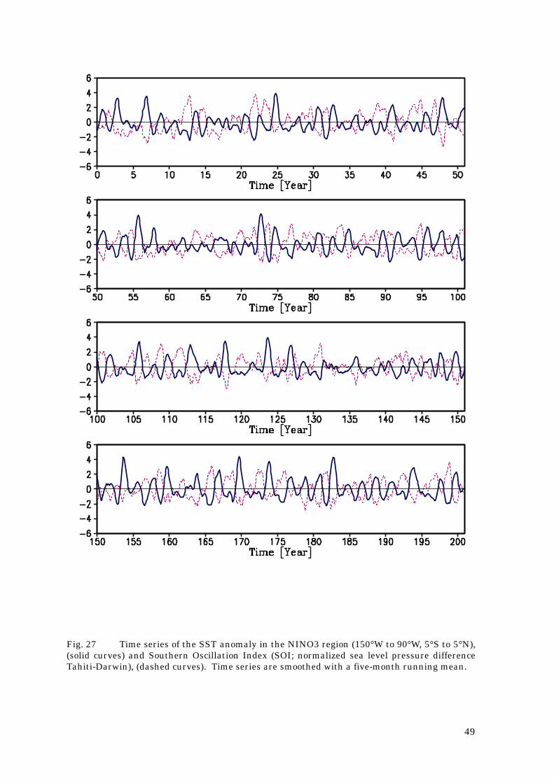
4.3 Model ENSO
The relatively large surface temperature variability in the equatorial Pacific shown in Fig. 24 implies ENSO variability in the model. Figure 27 shows the time series (with a 5-month running mean) of the SST anomaly in the NINO3 region (150°W to 90°W, 5°S to 5°N) and the
Southern Oscillation Index (SOI: normalized sea level pressure difference Tahiti-Darwin). The SST anomaly in NINO3 shows interannual variation with large amplitude from –2.5°C to +4°C. The peak value of +4°C is larger than the observed maximum value (about +3.6°C in the 1997/98 El Niño). It is noted that the SST anomaly shows larger positive peaks than negative peaks as for observed El Niño and La Niña. The time series shows a two-year oscillation with small amplitude is dominant in general, but large positive peaks are typically seen in three- to five-year intervals in some periods (e.g., years 100 to 130). This indicates the model is capable of simulating amplitude and frequency modulation of ENSO. It is clearly apparent that the SOI time series has a negative correlation with the NINO3 SST time series, which is consistent with the observed ENSO. The correlation coefficient is –0.72.
The geographical distribution of the SST anomaly regressed on the NINO3 SST is shown in Fig. 28, for observation (GISST2.2, Rayner et al., 1996), MRI-CGCM1 and MRI-CGCM2. In MRI-CGCM2, a prominent positive anomaly is seen in the central eastern equatorial Pacific, extending to the coast of Peru. This pattern is similar to the observed El Niño. In MRI-CGCM1, there was a westward-displaced maximum SST anomaly with its center to the west of the date line. However, it is improved and simulated around 150°W in the new model. In the former model (MRI-CGCM1), there is a negative anomaly in the eastern equatorial Indian Ocean that is not seen in the observation. This bias is caused by an unrealistic equatorial upwelling in the eastern Indian Ocean. However, it is improved in the new model in association with the improvement of the eastward gradient of the equatorial thermocline in the Indian Ocean (Fig. 20). The improvements should contribute to a better simulation, such as the relationship between ENSO and the Asian Monsoon.
Other fields in the ocean and atmosphere show a consistent structure associated with the model ENSO. Figure 29a shows an ocean temperature anomaly in the vertical section along the equator (regression on the NINO3 SST), together with the climatology of the model 20°C isotherm. There is a positive anomaly in the eastern Pacific along the 20°C isotherm,

14
accompanied by a surface positive anomaly. With a lagged regression (not shown), eastward propagation of the temperature anomaly in the upper thermocline is evident in the model, which implies propagation of Kelvin waves as a part of the evolution of El Niño.
The anomalies of 850 hPa wind and precipitation in the model El Niño are also shown in Fig. 29. In the equatorial region, a westerly wind anomaly is dominant in the central-western Pacific. The negative SST anomaly in the central North Pacific could be related to the intensified westerly wind associated with midlatitude atmospheric response to tropical convective activity change in ENSO (Horel and Wallace, 1981). The precipitation increases notably in the equatorial central-eastern Pacific and decreases around the ITCZ and SPCZ in the western Pacific. The model simulates a positive anomaly on the coast of Peru and a negative anomaly in northeastern Brazil, accompanying an easterly wind anomaly over northern South America. These are coherent and consistent with features typically seen in the observed El Niño. A detailed analysis for the model ENSO and associated variations will be demonstrated in a separate paper.
5. Summary and Discussion
A new version of the global atmosphere-ocean coupled general circulation model (MRI-CGCM2) has been developed at MRI. The model can be used to explore climate change associated with anthropogenic forcings. We aimed to reduce the drawbacks of the former version of the model (MRI-CGCM1, Tokioka et al., 1996) and achieve more realistic climatic mean and variability to predict climate changes with greater accuracy and reliability.
The model shows generally good performance, reproducing representative aspects of the mean climate and seasonal variation including surface air temperature, precipitation, snow and sea ice distribution, and ocean structure and circulation. In particular, sea ice distribution is much improved. The improvement of sea ice distribution in the NH is mainly due to appropriately simulated thermohaline circulation in the North Atlantic and careful tuning of the flux adjustment in the sea ice region. The seasonal extent of snow cover is
also simulated reasonably well. Climatic drift is substantially absent
in the model for a time period of the order of hundreds of years with respect to atmosphere, sea ice, SST and the upper ocean. The older version (MRI-CGCM1) showed a relatively large trend in tropical SST and sea ice volume. Such progress was important in the development of the new version for experiments studying long-term climate changes. A long coupled spin-up of the model is essential to stabilize the coupled integration. In addition to an asynchronous coupled spin-up, we used a further, synchronous, coupled spin-up of more than 100 years. The coupled spin-up in the former simulation (Tokioka et al., 1996) was only 30 years long, following separate spin-ups of the OGCM and the AGCM, restoring the observed climatology of SST and sea surface salinity. Careful treatment in the spin-up prior to the model control simulation is very important.
It has been suggested that the meridional overturning in the Atlantic Ocean contributes to the reduced rate of warming in the northern Atlantic associated with global warming (IPCC, 1996). It has been argued in many studies that the variation of the Atlantic overturning is a critical factor in the climate variability of the North Atlantic. Although MRI-CGCM1 failed in simulating the meridional overturning in the Atlantic Ocean, the present model shows a realistic value of 17 Sv near 54°N at 1500m depth. The improvement is principally due to the introduction of isopycnal mixing parameterization (with smaller lateral diffusivity), from which a strong density gradient around the fronts in the North Atlantic Ocean can be simulated in the model. The strong fronts lead to the strong North Atlantic Current that carries warm saline water to the Nordic Seas, producing a realistic sea ice distribution. This results in deep convections in the sea-ice-free region by strong atmospheric cooling, and consequently feeds a density flux to the North Atlantic Deep Water. The overturning in the model shows noteworthy interannual and interdecadal variability that should be investigated in detail in the future.
The model simulates not only realistic mean climate but also variabilities in both the atmosphere and the ocean, such as AO and ENSO. The dominant modes of atmospheric variability, as indicated by sea

15
level pressure (Fig. 26), are consistent with observation. Temporal variation of the SST anomaly in the NINO3 region shows a large positive value (max. +4°C) over several-year intervals. The SST anomaly pattern regressed on NINO3 SST (Fig. 28) shows a strong positive anomaly in the central-eastern equatorial Pacific that is similar to the observed El Niño. The corresponding temperature anomaly in the upper ocean along the equator shows a realistic east-west seesaw around the 20°C isotherm. The performance in simulating ENSO together with the sufficiently small climatic drift in the model implies that the model is suitable for studying changes of ENSO variability associated with climate changes like global warming.
The model still has some problems at present. The surface air temperature in winter at high latitude has a warm bias due to weaker stability in the boundary layer. We tested the sensitivity of the atmospheric model to a lower limit of vertical diffusivity in the case of strong stability, and found that winter temporal inversions at high latitude are well simulated in the model. We expect that adjusting the parameter will improve the warm bias in high latitudes in winter. However, it requires a long spin-up of the model to make another control run because even a small change will break the atmosphere-ocean coupled equilibrium.
The surface temperature over land in summer also shows a warm bias associated with a land process scheme problem. It appears that the soil moisture (not shown) becomes too low over the continent where the summer temperature becomes much higher than observed. The lack of surface soil moisture leads to a large sensible heat flux (small latent heat flux) from the ground in order to balance incoming solar radiation in summer. The low soil moisture in summer is probably related to a problem in the hydrological process, in which snow-melt water cannot be held in the soil layer in spring.
Although snow cover in winter is adequately simulated, the melting season is earlier than observed (Fig. 12). The snowmelt process is very sensitive to the albedo of snow since solar radiation is generally dominant in the surface energy balance at high latitude in spring. On the other hand, snow albedo differs very much with the condition of snow (e.g. past record of snow) that is related to various complicated processes. In the present model, however, snow is treated as a single layer, and its albedo is determined simply in relation to its
surface temperature (0.6 if near 0°C, otherwise 1.0). More sophisticated modeling of snow (multi-layered, and taking past snow records into account) is under development at present.
These problems require further careful consideration in the next improvements of the model. Acknowledgments
The authors thank the members of the Climate Research Department of MRI for their contribution to the development of the model. The present study is part of the special project on the prediction of global warming of the Japan Meteorological Agency. Some of the computing was supported by the Center for Global Environmental Research of the National Institute for Environmental Studies, Environmental Agency of Japan.
References
Arakawa, A. and W. H. Schubert, 1974: Interaction of a cumulus cloud ensemble with the large scale environment, Part I. J. Atmos. Sci., 31313131, 674-701.
Bourk, R. H. and R. P. Garrett, 1987: Cold Region Sci. Tech., 13131313, 259-280.
Da Silva, A., C. Young, and S. Levitus, 1994: Atlas of Surface Marine Data 1994, Vol. 1: Algorithms and Procedures. NOAA Atlas NESDIS 6-9. U.S. Gov. Printing Office, Wash., D.C., 83 pp.
Gent, P. R. and J. C. McWilliams, 1990: Isopycnal mixing in ocean circulation models. J. Phys. Oceanogr., 20202020, 150-155.
Gleckler, P. J., D. A. Randall, G. Boer, R. Colman, M. Dix, V. Galin, M. Helfand, J. Kiehl, A. Kitoh, W. Lau, X.-Y. Liang, V. Lykossov, B. McAvaney, K. Miyakoda, S. Planton, and W. Stern, 1995: Cloud-radiative effects on implied oceanic energy transports as simulated by atmospheric general circulation models. Geophys. Res. Lett., 22222222, 791-794.
Hellerman, S. and M. Rosenstein, 1983: Normal monthly wind stress over the world's ocean with error estimates. J. Phys. Oceanogr., 13131313, 1093-1104.
Horel, J. D., and J. M. Wallace, 1981: Planetary-scale atmospheric phenomena associated with the Southern Oscillation, Mon. Weather Rev., 109109109109, 813-829.

16
IPCC, 1996: Climate change 1995, The science of climate change. Eds. J. T. Houghton, L. G. Meira Filho, B. A. Callander, N. Harris, A. Kattenberg and K. Maskell. Cambridge Univ. Press, 570pp.
Iwasaki, T., S. Yamada and K. Tada, 1989: A parameterization scheme of orographic gravity wave drag with the different vertical partitioning, part 1: Impact on medium range forecasts. J. Meteor. Soc. Japan, 67676767, 11-41.
Jones, P. D., 1994: Hemispheric surface air temperature variations: A reanalysis and update to 1993. J. Climate, 7777, 1794-1802.
Kalney, E. and Co-authors, 1996: The NCEP/NCAR 40-year Reanalysis Project. Bull. Amer. Meteor. Soc., 77777777, 437-471.
Kitoh, A., S. Yukimoto, and A. Noda, 1999: ENSO-monsoon relationship in the MRI coupled GCM. J. Meteor. Soc. Japan, 77777777, 1221-1245.
Kitoh, A., S. Yukimoto, A. Noda, and T. Motoi, 1997: Simulated changes in the Asian summer monsoon at times of increased atmospheric CO2. J. Meteor. Soc. Japan, 75757575, 1019-1031.
Lacis, A. A. and J. E. Hansen, 1974: A parameterization for the absorption of solar radiation in the Earth’s atmosphere. J. Atmos. Sci., 31313131, 118-133.
Levitus, S. and T. P. Boyer, 1994: World Ocean Atlas, Volume 4: Temperature, NOAA Atlas NESDIS 4, 129 pp.
Levitus, S., R. Burgett, and T. P. Boyer, 1994: World Ocean Atlas, Volume 3: Salinity, NOAA Atlas NESDIS 3, 111 pp.
Mellor, G. L. and P. A. Durbin, 1975: The structure and dynamics of the ocean surface mixed layer. J. Phys. Oceanogr., 5555, 718-728.
Mellor, G. L. and L. Kantha, 1989: An ice-ocean coupled model. J. Geophys. Res., 94949494, 10937-10954.
Mellor, G. L. and T. Yamada, 1974: A hierarchy of turbulence closure models for planetary boundary layers. J. Atmos. Sci., 31313131, 1791-1806.
Mellor, G. L. and T. Yamada, 1982: Development of a turbulence closure model for geophysical fluid problems. Rev. Geophys. Space Phys., 20202020, 851-875.
Nitta, T., and S. Yamada, 1989: Recent warming of tropical sea surface temperature and its relationship to the Northern Hemisphere circulation. J.
Meteor. Soc. Japan, 67676767, 375-383. Noda, A., K. Yoshimatsu, A. Kitoh and H.
Koide, 1999a: Relationship between natural variability and CO2-induced warming pattern: MRI coupled atmosphere/mixed-layer ocean (slab) GCM experiment. 10th Symposium on Global Change Studies, 10-15 January 1999, Dallas, Texas., pp.355-358, American Meteorological Society, Boston. Mass.
Noda, A., K. Yoshimatsu, S. Yukimoto, K. Yamaguchi, and S. Yamaki, 1999b: Relationship between natural variability and CO2-induced warming pattern: MRI AOGCM atmosphere/mixed-layer ocean (slab) GCM experiment. 10th Symposium on Global Change Studies, 10-15 January 1999, Dallas, Texas, pp.359-362, American Meteorological Society, Boston. Mass.
Palmer, T. N., G. N. Shutts and R. Swinbank, 1986: Alleviation of a systematic westerly bias in general circulation and numerical weather prediction models through an orographic gravity wave drag parameterization. Quart. J. Roy. Meteor. Soc., 112112112112, 1001-1039.
Perovich, D. K., G. A. Maykut and T. C. Grenfell, 1986: Optical properties of ice and snow in the polar oceans, I. Observations. Proc. SPIE Int. Soc. Opt. Eng., 637637637637, 232-241.
Rayner, N. A., Horton, E. B., Parker, D. E., Folland, C. K. and Hackett, R. B. 1996: Version 2.2 of the Global Sea-Ice and Sea Surface Temperature data set, 1903-1994. Climate Research Technical Note 74.
Randall, D. and D.-M. Pan, 1993: Implementation of the Arakawa-Schubert cumulus parameterization with a prognostic closure. Meteorological Monograph/The representation of cumulus convection in numerical models, 46, 145-150.
Read, J. F. and R. T. Pollard, 1993: Structure and transport of the Antarctic circumpolar current and Agulhas return current at 40°E. J. Geophys. Res., 98989898, 12281-12295.
Robinson, D. A., K. F. Dewey and R. R. Heim, Jr., 1993: Global snow cover monitoring: An update. Bull. Amer. Meteor. Soc., 74747474, 1689-1696.
Sato, N., P. J. Sellers, D. A. Randall, E. K. Schneider, J. Shukla, J. L. Kinter, Y.-Y.

17
Hou and E. Albertazzi, 1989: Effects of implementing the simple biosphere model in a general circulation model. J. Atmos. Sci., 46464646, 2757-2782.
Schmitz, W. J. Jr. and M. S. McCartney, 1993: On the north Atlantic circulation. Rev. Geophys., 31 31 31 31, 29-49.
Sellers, P. J., Y. Mintz, Y. C. Sud and A. Dalcher, 1986: A simple biosphere model (SiB) for use within general circulation models. J. Atmos. Sci., 43434343, 505-531.
Shibata, K. and T. Aoki, 1989: An infrared radiative scheme for the numerical models of weather and climate. J. Geophys. Res., 94949494, 14923-14943.
Shibata, K. and A. Uchiyama, 1992: Accuracy of the delta-four-stream approximation in inhomogeneous scattering atmospheres. J. Meteor. Soc. Japan, 70707070, 1097-1109.
Shibata, K., H. Yoshimura, M. Ohizumi, M. Hosaka and M. Sugi, 1999: A simulation of troposphere, stratosphere and mesosphere with an MRI/JMA98 GCM. Pap. Meteor. Geophys., 50505050, 15-53.
Thompson, D. W. J. and J. M. Wallace, 1998: The Arctic oscillation signature in the wintertime geopotential height and temperature fields. Geophys. Res. Lett., 25252525, 1297-1300.
Tokioka T., A. Noda, A. Kitoh, Y. Nikaidou, S. Nakagawa, T. Motoi, S. Yukimoto and K. Takata, 1996: A transient CO2 experiment with the MRI CGCM – Annual mean response. CGER's supercomputer monograph report, 2, Center for Global Environmental Research, National Institute for Environmental Studies, Environmental Agency of Japan.
Tokioka, T., K. Yamazaki, A. Kitoh and T. Ose, 1988: The equatorial 30-60 day oscillation and the Arakawa-Schubert penetrative cumulus parameterization. J. Meteor. Soc. Japan, 66666666, 883-901.
Trenberth, K. E., 1998: The heat budget of the atmosphere and ocean. Proceedings of the First WCRP International Conference on Reanalysis, WMO/TD-No. 876, 17-20.
Wang, W.-C., X.-Z. Ling, M. P. Dudek, D. Pollard and S. L. Thompson, 1995: Atmospheric ozone as a climate gas. Atmos. Res., 37373737, 247-256.
Xie, P. and P. A. Arkin, 1996: Analyses of global monthly precipitation using gauge observations, satellite estimates
and numerical model predictions. J. Climate, 9999, 4840-4858.
Yukimoto, S., M. Endoh, Y. Kitamura, A. Kitoh, T. Motoi, A. Noda, and T. Tokioka, 1996: Interannual and interdecadal variabilities in the Pacific in an MRI coupled GCM. Climate Dyn., 12121212, 667-683.
Yukimoto, S. M. Endoh, Y. Kitamura, A. Kitoh, T. Motoi, and A. Noda, 2000: ENSO-like interdecadal variability in the Pacific Ocean as simulated in a coupled general circulation model. J. Geophys. Res., 105105105105, 13,945-13,963.
18
Table 1. Comparison of MRI-CGCM1 and MRI-CGCM2
Aspect MRI- CGCM1 MRI-CGCM2 Atmospheric component Horizontal resolution 5°(long.) × 4°(lat.) T42 (~2.8° × 2.8°) Layer (top) 15 (1hPa) 30 (0.4hPa) Solar radiation Lacis and Hansen (1974) Shibata and Uchiyama (1992) (SW) H2O, O3 H2O, O3, aerosol Long-wave radiation Shibata and Aoki (1989) Shibata and Aoki (1989) (LW) H2O, CO2, O3 H2O, CO2, O3, CH4, N2O Convection Arakawa and Schubert (1974) Prognostic Arakawa-Schubert Randall and Pan (1993) Planetary Boundary Layer Bulk layer (Tokioka et al., 1988) Mellor and Yamada (1974) (PBL) Gravity wave drag Palmer et al. (1986) Iwasaki et al. (1989) Rayleigh friction Rayleigh friction Cloud type Penetrative convection, Penetrative convection Middle-level convection, Large-scale condensation, Large-scale condensation Stratus in PBL Cloudiness Saturation function of relative humidity Cloud overlap random for non-convective clouds random + correlation 0.3 for convective clouds Cloud water content function of pressure and function of temperature temperature Land process 4-layer diffusion model 3-layer SiB Oceanic component Horizontal resolution 2.5° (lon.) × 2°-0.5° (lat.) Layer (min. thickness) 21 (5.2m) 23 (5.2m) Eddy viscosity Horiz. visc. 2.0×10⁵ m2s–1 Horiz. visc. 1.6×10⁵ m2s–1
Vert. visc. 1×10⁻⁴ m2s–1 Vert. visc. 1×10⁻⁴ m2s–1 Eddy mixing Horizontal-vertical mixing Isopicnal mixing + Gent and McWilliams (1990) Horiz. diff. 5.0×10³ m2s–1 Isopycnal 2.0×10³ m2s–1
Vert. diff. 5.0×10⁻⁵m2s–1 Diapycnal 1.0×10⁻⁵ m2s–1 Vertical viscosity and Mellor and Yamada (1974, 1982) diffusivity Sea ice Mellor and Kantha (1989) Atmosphere-ocean coupling Coupling interval 6 hours 24 hours Flux adjustment heat, salinity heat, salinity + wind stress (12°S-12°N)
19
Table 2. Vertical level spacing in the ocean model of MRI-CGCM2 Level Level spacing (m) Depth of level center
(m) Depth of level bottom
(m) 1 5.2 2.8 5.2 2 6.2 8.3 11.4 3 7.9 15.35 19.3 4 10.7 24.65 30.0 5 25.0 42.5 55.0 6 25.0 67.5 80.0 7 25.0 92.5 105.0 8 25.0 117.5 130.0 9 25.0 142.5 155.0
10 25.0 167.5 180.0 11 30.0 195.0 210.0 12 40.0 230.0 250.0 13 50.0 275.0 300.0 14 100.0 350.0 400.0 15 200.0 500.0 600.0 16 200.0 700.0 800.0 17 300.0 950.0 1100.0 18 400.0 1300.0 1500.0 19 700.0 1850.0 2200.0 20 700.0 2550.0 2900.0 21 700.0 3250.0 3600.0 22 700.0 3950.0 4300.0 23 700.0 4650.0 5000.0

20
Table 3. Spin-up runs for the control run
Run Model Prescribed forcing data Integration period (years)
Forcing data output for the subsequent run (averaged years)
SPIN-UP1 OGCM SSTo, SSSo, TAUo, Sio 24 -- SPIN-UP2 AGCM SSTo, Sio 24 Flux-A1 (10) SPIN-UP3 OGCM Flux-A1, SSTo, SSSo, TAUo, SIo 30 -- SPIN-UP4 AGCM SST-O2, Sio 16 Flux-A2 (10) SPIN-UP5 OGCM Flux-A2, SSTo, SSSo, TAUo, SIo 155 -- SPIN-UP6 CGCM SSTo, SSSo, TAUo, Sio 65 Fadj-C1 (10) SPIN-UP7 CGCM Fadj-C1, Sio 17 -- SPIN-UP8 CGCM Fadj-C1 29 -- CONTROL CGCM Fadj-C1 201 -- SSTo: Observed climatological sea surface temperature (Levitusand Boyer, 1994) SSSo: Observed climatological sea surface salinity (Levitus et al., 1994) TAUo: Observed climatological surface wind stress (Hellerman and Rosenstein, 1983) SIo: Observed climatological sea ice distribution (SIGRID by Navy-NOAA Joint Ice Center, Bourke and Garrett, 1987) Flux-run: Climatological surface fluxes (for heat, freshwater and momentum) obtained from the run SST-run: Climatological sea surface temperature obtained from the run Fadj-run: Climatological flux adjustment (for heat, freshwater and momentum) obtained from the run

21
Fig. 1 Climatological annual mean heat flux adjustments (Wm-2) in (a) MRI- CGCM2 and (b) MRI-CGCM1, and freshwater flux adjustments (mm/day) in (c) MRI- CGCM2 and (d) MRI-CGCM1.

Fig. 2 Zonally averaged net surface heat flux for (a) December-February (DJF) mean and (b) June-August (JJA) mean, and freshwater fluxfor (c) DJF and (d) JJA. (solid: observation, long-dash: atmospheric model, short-dash: flux adjustment, dot-dash: model adjusted). Theobserved heat flux is from Da Silva et al. (1994), and freshwater flux for the observation is estimated by precipitation (Xie and Arkin, 1996) minusevaporation (Da Silva et al., 1994).

23
Fig. 3 Wind stress along the equator (averaged in the 4°S-4°N band), calculated by the atmospheric model (dashed curve) and adjusted(solid curve) for January (a, zonal component; b, meridional component) and July. (c, zonal component; d, meridional component). Unit isNm-2.

Fig. 4 Annual mean northward energy transports by the ocean (solid) and the atmosphere (dashed) in (a) MRI-CGCM2 and (b) MRI-CGCM1. The atmospheric transports are implied from differences between the net fluxes atthe top-of-the-atmosphere and the sea surface (including flux adjustment).Unit is PW.
24

Fig. 5 Horizontal distribution of the net surface heat flux for DJF mean (a, observation; b, MRI-CGobservation; d, MRI-CGCM2). Unit is Wm-2.
25
CM2) and for JJA mean (c,


27
Fig. 7 Vertical profiles of the zonal mean air temperature at 80°N in winter (DJF) for the model(solid) and observation (dashed, NCEP/NCAR reanalysis climatology for 1979 to 1995).

8
2Fig. 8 Time series of the annual mean surface air temperature globallyaveraged over (a) land, (b) ocean, (c) land+ocean simulated by MRI-CGCM2, and(d) land+ocean simulated by MRI-CGCM1. Thin lines denote the linear trends foreach time series.

29 Fig. 9 Climatology of the mean sea level pressure for DJF (a, MRI-CGCM2; b, observation) and JJA (c, MRI-CGCM2; d: observation). The observations are from NCEP/NCAR reanalysis climatology for 1979 to 1995. Contour interval is 4 hPa.

30
Fig. 10 As in Fig. 9, but for the precipitation. Contour levels are 2, 4, 8, and 12 mm/day-1. The observations are from Xie and Arkin (1996).

31 Fig. 11 Climatology of seasonal variation of snow cover extent over land in the Northern Hemisphere for MRI-CGCM2 (left panels) and observation (right panels, NOAA/SIGRID, 1967-87), for October (upper), January (middle) and April (lower). Values arepercentages.
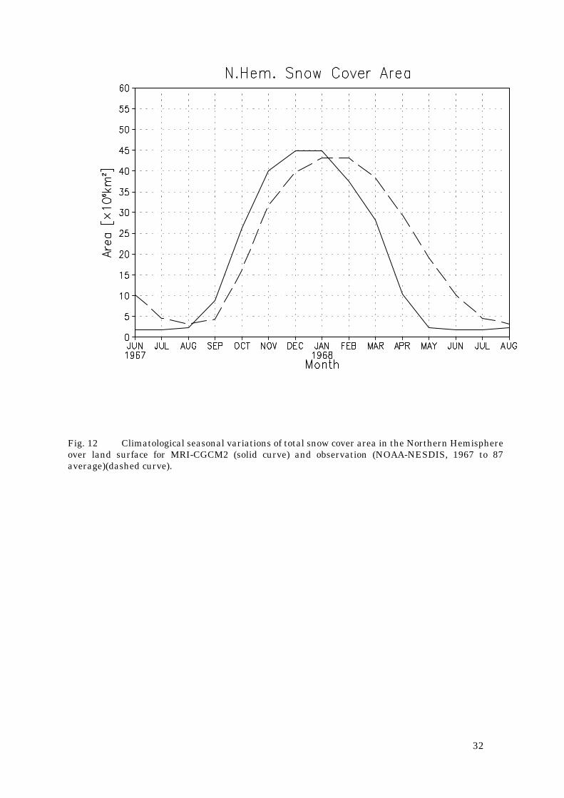
Fig. 12 Climatological seasonal variations of total snow cover area in the Northern Hemisphere over land surface for MRI-CGCM2 (solid curve) and observation (NOAA-NESDIS, 1967 to 87 average)(dashed curve).
32

33 Fig. 13 Climatology of the sea surface temperature for January to March (JFM) mean (a, MRI-CGCM2; b: model–observation) and July to September (JAS) mean (c, MRI-CGCM2; d, model–observation). The observation is from Levitus and Boyer (1994).

34
Fig. 14 Climatology of the annual mean sea surface salinity for (a)MRI-CGCM2 and (b) difference between MRI-CGCM2 and observation (Levitus et al., 1994).


36
Fig. 16 Climatology of the oceanic barotropic stream functions (in Sv) ofMRI-CGCM2 for (a) JFM mean and (b) JAS mean.
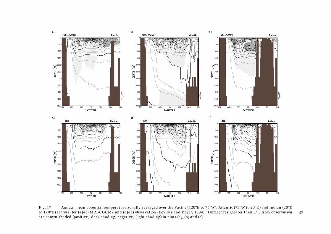
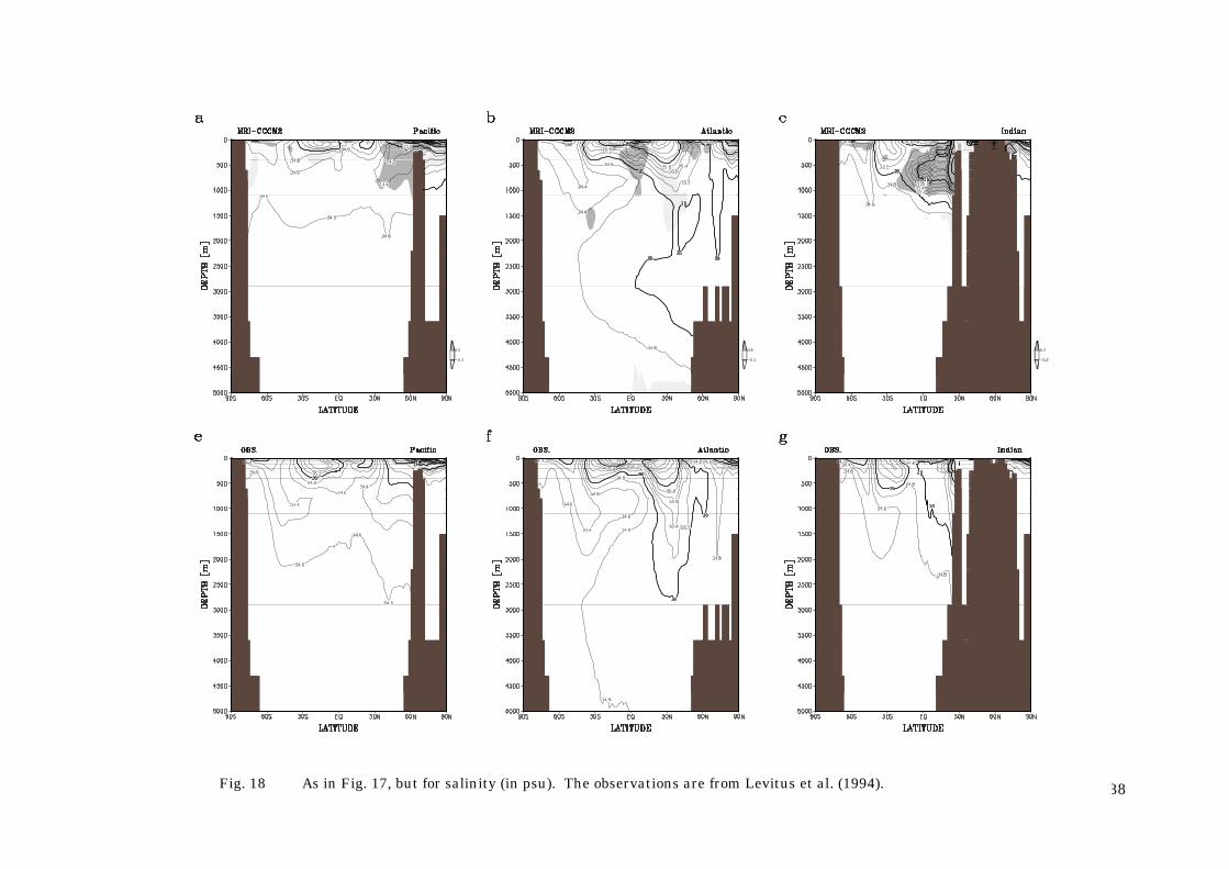
Fig. 18 As in Fig. 17, but for salinity (in psu). The observations are from Levitus et al. (1994).
38
39
Fig. 19 Annual mean meridional overturning stream functions for the global ocean in (a) MRI-CGCM1 and (b) MRI-CGCM2. Time series of the maximum (annual mean) meridional overturning in the North Atlantic Ocean for (c) MRI-CGCM1 and (d) MRI-CGCM2. Values are in Sv.

Fig. 20 Annual mean potential temperature along the equator (averaged 2°S to 2°N)for (a) MRI-CGCM2 and (b) observation (Levitus and Boyer, 1994). The differences fromthe observations larger than 1°C are shown with shading (positive, dark shading; negative,light shading) in plot (a).
40

Fig. 21-1 Geographical distribution of climatological sea ice compactness (contour, unit: percent) and meaNorthern Hemisphere (NH) for March (a, MRI-CGCM2; b, observation) and September (c, MRI-CGCM2; d, obare from NOAA-SIGRID for compactness, and Bourk and Garrett (1987) for thickness.
41
n thickness (shading) in theservation). The observations

42 Fig. 21-2 Same as Fig. 20-1, except for the Southern Hemisphere (SH). Only compactness is shown for the observation.

43
Fig. 21-3 Geographical distribution of climatological sea ice compactness (unit: percent) in MRI-CGCM1 for (i) March and (j) September.

44
Fig. 22 Seasonal variations of sea ice area (a, NH; b, SH) and volume (c, NH; d, SH) for MRI-CGCM2 (solid curves) and observation (dashed curves). The observation of sea ice volume is shown only for the NH.
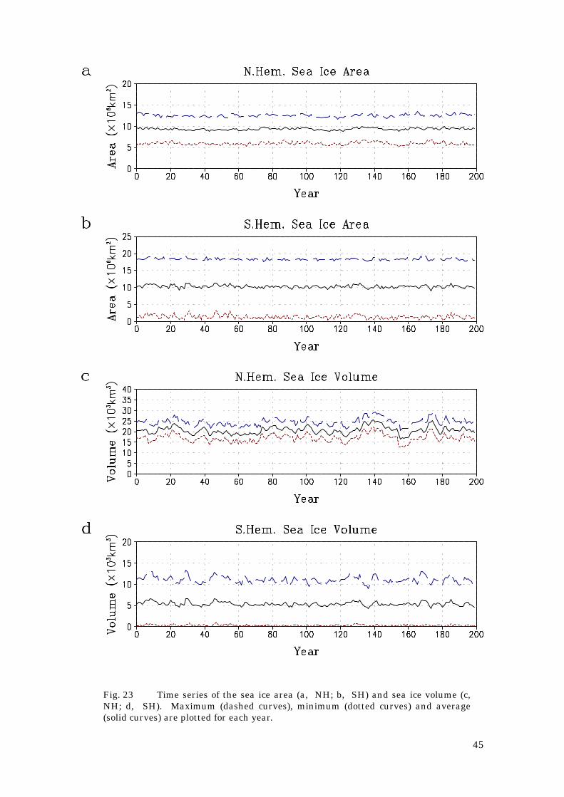
Fig. 23 Time series of the sea ice area (a, NH; b, SH) and sea ice volume (c,NH; d, SH). Maximum (dashed curves), minimum (dotted curves) and average(solid curves) are plotted for each year.
45

Fig. 24 Standard deviation of surface air temperature for the December-February (DJF) meaobservation), and the June-August (JJA) mean (c, MRI-CGCM2; d, observation). Observations are calcudata (Jones, 1994).
46
n (a, MRI-CGCM2; b, lated from 1947 to 1998

47 Fig. 25 As in Fig. 24, but for mean sea level pressure. Observations are from NCEP/NCAR-reanalysis for 1950-1995.

F(N
48
ig. 26 The leading four EOF modes of mean sea level pressure in the Northern Hemisphere for DJF. (a)-(d) model and (e)-(h) observation CEP/NCAR-reanalysis for 1950 to 1995). Contour values indicate variance in (hPa)2.
49
Fig. 27 Time series of the SST anomaly in the NINO3 region (150°W to 90°W, 5°S to 5°N),(solid curves) and Southern Oscillation Index (SOI; normalized sea level pressure differenceTahiti-Darwin), (dashed curves). Time series are smoothed with a five-month running mean.

Fig. 28 Sea surface temperature anomaly regressed on the normalized time series of the SST in the NINO3 region, for (a) observation (GISST2.2), (b)MRI-CGCM1 and (c) MRI-CGCM2.

Fig. 29 (a) Ocean temperature anomaly in the equator section regressed on the normalized time seriesregion. Dashed curve indicates climatological 20°C isotherm in the model. Similar regression for (b) wind anovector indicates 1 ms–1) and (c) precipitation anomaly (negative shaded, contour interval is 0.5 mm/day).
51
of the SST in the NINO3maly at 850 hPa (reference