Embed Size (px)
Citation preview
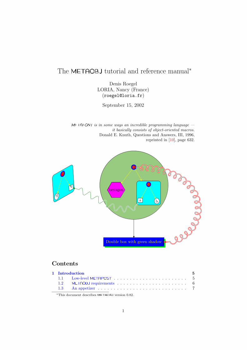
The metaobj tutorial and reference manual∗
Denis RoegelLORIA, Nancy (France)
September 15, 2002
metafont is in some ways an incredible programming language —it basically consists of object-oriented macros.
Donald E. Knuth, Questions and Answers, III, 1996,reprinted in [10], page 632.
Double box with green shadow
hexagon
a b
c
c
a
b
c
Contents
1 Introduction 51.1 Low-level metapost . . . . . . . . . . . . . . . . . . . . . . . 51.2 metaobj requirements . . . . . . . . . . . . . . . . . . . . . . 61.3 An appetizer . . . . . . . . . . . . . . . . . . . . . . . . . . . . 7
∗This document describes metaobj version 0.82.
1
1.4 What is an object? . . . . . . . . . . . . . . . . . . . . . . . . . 81.4.1 A name . . . . . . . . . . . . . . . . . . . . . . . . . . . . 81.4.2 Points . . . . . . . . . . . . . . . . . . . . . . . . . . . . . 91.4.3 Equations . . . . . . . . . . . . . . . . . . . . . . . . . . . 91.4.4 Pictures . . . . . . . . . . . . . . . . . . . . . . . . . . . . 101.4.5 Paths . . . . . . . . . . . . . . . . . . . . . . . . . . . . . 101.4.6 Subobjects . . . . . . . . . . . . . . . . . . . . . . . . . . 111.4.7 Other components . . . . . . . . . . . . . . . . . . . . . . 11
1.5 Transformations . . . . . . . . . . . . . . . . . . . . . . . . . . 11
2 A first object 122.1 A segment . . . . . . . . . . . . . . . . . . . . . . . . . . . . . 122.2 Connecting two objects . . . . . . . . . . . . . . . . . . . . . . 142.3 Creating an object containing objects . . . . . . . . . . . . . . 16
3 Interfaces and reusability 213.1 Standard points . . . . . . . . . . . . . . . . . . . . . . . . . . 213.2 Standard equations . . . . . . . . . . . . . . . . . . . . . . . . 22
4 Real examples 27
5 Advanced operations 325.1 Streamlined constructors . . . . . . . . . . . . . . . . . . . . . 325.2 Cloning . . . . . . . . . . . . . . . . . . . . . . . . . . . . . . . 335.3 Fiddling with the bounding box . . . . . . . . . . . . . . . . . 33
5.3.1 BB: a new bounding box layer . . . . . . . . . . . . . . . . 345.3.2 Rebinding an object . . . . . . . . . . . . . . . . . . . . . 34
5.4 Unattaching an object . . . . . . . . . . . . . . . . . . . . . . . 355.5 Options . . . . . . . . . . . . . . . . . . . . . . . . . . . . . . . 35
5.5.1 Syntax . . . . . . . . . . . . . . . . . . . . . . . . . . . . . 355.5.2 Option types . . . . . . . . . . . . . . . . . . . . . . . . . 365.5.3 Option definition . . . . . . . . . . . . . . . . . . . . . . . 375.5.4 Option names . . . . . . . . . . . . . . . . . . . . . . . . . 37
5.6 Adding paths to objects . . . . . . . . . . . . . . . . . . . . . . 375.7 Connections . . . . . . . . . . . . . . . . . . . . . . . . . . . . 39
5.7.1 ncline . . . . . . . . . . . . . . . . . . . . . . . . . . . . 425.7.2 nccurve . . . . . . . . . . . . . . . . . . . . . . . . . . . . 445.7.3 ncarc . . . . . . . . . . . . . . . . . . . . . . . . . . . . . 455.7.4 ncbar . . . . . . . . . . . . . . . . . . . . . . . . . . . . . 455.7.5 ncangle . . . . . . . . . . . . . . . . . . . . . . . . . . . . 465.7.6 ncangles . . . . . . . . . . . . . . . . . . . . . . . . . . . 465.7.7 ncdiag . . . . . . . . . . . . . . . . . . . . . . . . . . . . 475.7.8 ncdiagg . . . . . . . . . . . . . . . . . . . . . . . . . . . . 485.7.9 ncloop . . . . . . . . . . . . . . . . . . . . . . . . . . . . 485.7.10 nccircle . . . . . . . . . . . . . . . . . . . . . . . . . . . 505.7.11 ncbox . . . . . . . . . . . . . . . . . . . . . . . . . . . . . 505.7.12 ncarcbox . . . . . . . . . . . . . . . . . . . . . . . . . . . 515.7.13 nczigzag and nccoil . . . . . . . . . . . . . . . . . . . . 525.7.14 Tree and matrix variants . . . . . . . . . . . . . . . . . . 53
5.8 Adding labels . . . . . . . . . . . . . . . . . . . . . . . . . . . . 54
2
6 The object structure 56
7 Standard Library – Gallery 597.1 Basic objects . . . . . . . . . . . . . . . . . . . . . . . . . . . . 59
7.1.1 EmptyBox . . . . . . . . . . . . . . . . . . . . . . . . . . . 597.1.2 HRazor . . . . . . . . . . . . . . . . . . . . . . . . . . . . 607.1.3 RandomBox . . . . . . . . . . . . . . . . . . . . . . . . . . 60
7.2 Basic containers . . . . . . . . . . . . . . . . . . . . . . . . . . 617.2.1 Box . . . . . . . . . . . . . . . . . . . . . . . . . . . . . . 617.2.2 Polygon . . . . . . . . . . . . . . . . . . . . . . . . . . . . 627.2.3 Ellipse . . . . . . . . . . . . . . . . . . . . . . . . . . . . 637.2.4 Circle . . . . . . . . . . . . . . . . . . . . . . . . . . . . 647.2.5 DBox . . . . . . . . . . . . . . . . . . . . . . . . . . . . . . 657.2.6 DEllipse . . . . . . . . . . . . . . . . . . . . . . . . . . . 66
7.3 Box alignment constructors . . . . . . . . . . . . . . . . . . . . 677.3.1 HBox . . . . . . . . . . . . . . . . . . . . . . . . . . . . . . 677.3.2 VBox . . . . . . . . . . . . . . . . . . . . . . . . . . . . . . 69
7.4 Recursive objects and fractals . . . . . . . . . . . . . . . . . . 717.4.1 RecursiveBox . . . . . . . . . . . . . . . . . . . . . . . . 717.4.2 VonKochFlake . . . . . . . . . . . . . . . . . . . . . . . . 72
7.5 Trees . . . . . . . . . . . . . . . . . . . . . . . . . . . . . . . . 737.5.1 Tree . . . . . . . . . . . . . . . . . . . . . . . . . . . . . . 737.5.2 PTree . . . . . . . . . . . . . . . . . . . . . . . . . . . . . 82
7.6 Matrices . . . . . . . . . . . . . . . . . . . . . . . . . . . . . . 897.6.1 Experimental constructions . . . . . . . . . . . . . . . . . 907.6.2 Matrices with brackets (experimental) . . . . . . . . . . . 917.6.3 Matrix with labels . . . . . . . . . . . . . . . . . . . . . . 927.6.4 Matrix options . . . . . . . . . . . . . . . . . . . . . . . . 92
7.7 PSTricks/metaobj gallery . . . . . . . . . . . . . . . . . . . . 93
8 Class builder manual 1148.1 Components of a class . . . . . . . . . . . . . . . . . . . . . . . 114
8.1.1 Constructor . . . . . . . . . . . . . . . . . . . . . . . . . . 1148.1.2 Streamlined constructor . . . . . . . . . . . . . . . . . . . 1168.1.3 Bounding path . . . . . . . . . . . . . . . . . . . . . . . . 1168.1.4 Drawing function . . . . . . . . . . . . . . . . . . . . . . . 1168.1.5 Alternate constructors . . . . . . . . . . . . . . . . . . . . 1168.1.6 Additional functions . . . . . . . . . . . . . . . . . . . . . 1178.1.7 Option declarations . . . . . . . . . . . . . . . . . . . . . 1178.1.8 Default values for options . . . . . . . . . . . . . . . . . . 118
8.2 Design rules . . . . . . . . . . . . . . . . . . . . . . . . . . . . 118
9 Non-linear transformations on objects 1199.1 Simple transformations which do not change the layout . . . . 119
9.1.1 Example 1: changing the frame color . . . . . . . . . . . . 1199.1.2 Example 2: changing the content of a label . . . . . . . . 120
9.2 Transformations that change the layout . . . . . . . . . . . . . 120
3
10 Comparison with other packages 12210.1 Compatibility with boxes.mp . . . . . . . . . . . . . . . . . . . 12210.2 fancybox package . . . . . . . . . . . . . . . . . . . . . . . . . 12210.3 PSTricks . . . . . . . . . . . . . . . . . . . . . . . . . . . . . . 122
11 Memory requirements – metapost bug 123
12 Using metaobj from within TEX 124
Conclusion 124
Acknowledgments 125
References 126
Index 128
4
1 Introduction
This manual describes metaobj, a system for high-level object-oriented draw-ing based on metapost. The name metaobj is short for “metapost Ob-jects.”
metapost [5, 6, 2] is a programming language for drawings. It was createdby John Hobby as an adaptation of Donald Knuth’s metafont system [9].
This manual is not an introduction to metapost and some familiarity withmetapost is assumed.
This section gives a general introduction to metaobj and to the motivationsthat led us to create it. We will first try to show that metaobj is a usefulapproach for complex structural drawing.
1.1 Low-level metapost
In “low-level” metapost, complex drawings can be simplified by well chosendefinitions and definitions that are well parameterized. For instance, a generalsquare can be defined with
def Square(expr p,l,a)=(p--(p+l*dir(a))--(p+l*dir(a)+l*dir(a+90))--(p+l*dir(a+90))--cycle)
enddef;
and it can then be drawn with
draw Square(origin,1cm,50);
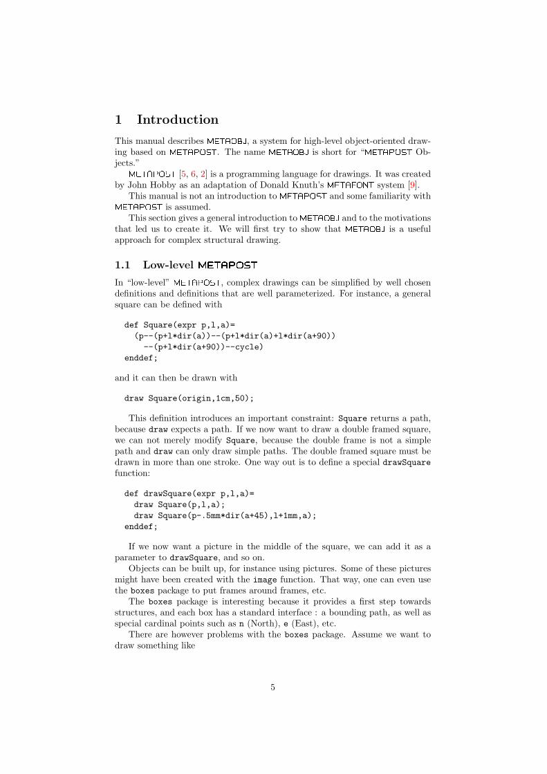
This definition introduces an important constraint: Square returns a path,because draw expects a path. If we now want to draw a double framed square,we can not merely modify Square, because the double frame is not a simplepath and draw can only draw simple paths. The double framed square must bedrawn in more than one stroke. One way out is to define a special drawSquarefunction:
def drawSquare(expr p,l,a)=draw Square(p,l,a);draw Square(p-.5mm*dir(a+45),l+1mm,a);
enddef;
If we now want a picture in the middle of the square, we can add it as aparameter to drawSquare, and so on.
Objects can be built up, for instance using pictures. Some of these picturesmight have been created with the image function. That way, one can even usethe boxes package to put frames around frames, etc.
The boxes package is interesting because it provides a first step towardsstructures, and each box has a standard interface : a bounding path, as well asspecial cardinal points such as n (North), e (East), etc.
There are however problems with the boxes package. Assume we want todraw something like
5

where all the rectangles are boxes created with the boxit function from theboxes package, and assume we want to connect point e of one subbox to pointw of the other, and obtain something like:
e w
We would like to use boxes or something similar because it provides a verysimple way to frame a picture. We do not want to have to place four cornersevery time we have to frame something. boxes instead provides a functionalapproach.
If we decide to make pictures of each subbox, and then somehow stuff theminside a boxit, we can’t achieve our task, because the positions of the pointsof interest to us have been lost. We could of course build the connection firstand put everything inside the larger box. That would work, but only becausethere is no connection from a subbox to another box outside our big box. So,no matter what we are doing, merely making a picture out of something freezesand anonymizes what is inside.
Achieving the previous drawing with the boxes package is as a matter offact tricky. One would like to use this package, but it doesn’t suit the task well.With boxes.mp we can put frames (rectangular or elliptic) around a picture,but we can’t go further without losing the structure.
1.2 metaobj requirements
The motivation that led to our work was exactly this: when we have severalobjects, such as boxes, and certain objects are inside others, we still want tohave access to the individual structures; we want to be able to reach any point,anything that’s inside.
Rather quickly, this apparently simple task became a more ambitious one,where we set ourselves to provide means to manipulate general structures inthe plane. At the same time, we want to keep the declarative features of thelanguage, as well as the functional approach of the boxes package. After manyexperiments, we found it desirable to meet the following requirements:
• our system should provide a notion of object and objects should be in-stances of classes so that several identical objects can easily be created;
6
• an object should be similar in behavior to a point, in that an object canbe put anywhere, and objects may or may not be completely defined, justlike points;
• in order to achieve the above, considering only the points constituting anobject, we have to define equations between these points;
• the objects should by default be rigid, with only two degrees of freedom(as in boxes), in the sense that the position of one point will determineall the other ones;
• it is interesting to have a boxes.mp-like interface, where an object o canbe positionned with something like o.c=origin;
• the objects should accept all linear transformations by default, that is, wemust be able to move, rotate, slant, etc., our objects, and yet keep theequations defining the objects, so that after any such linear transforma-tion, the object can still be put anywhere with a mere o.c=...
• we must have composition, that is, it must be possible to put objectsinside objects;
• paths and pictures must be able to be part of an object;
• when an object contains another object, the subobject should be repla-cable by any other object; that is, the class of an object should not, ifpossible, influence its use.
• all constituents should be reachable;
• the objects should be customizable, for instance through options;
• a library of classes should be provided and the creation of new classesshould be made simple
The metaobj package addresses all these issues and many others.
1.3 An appetizer
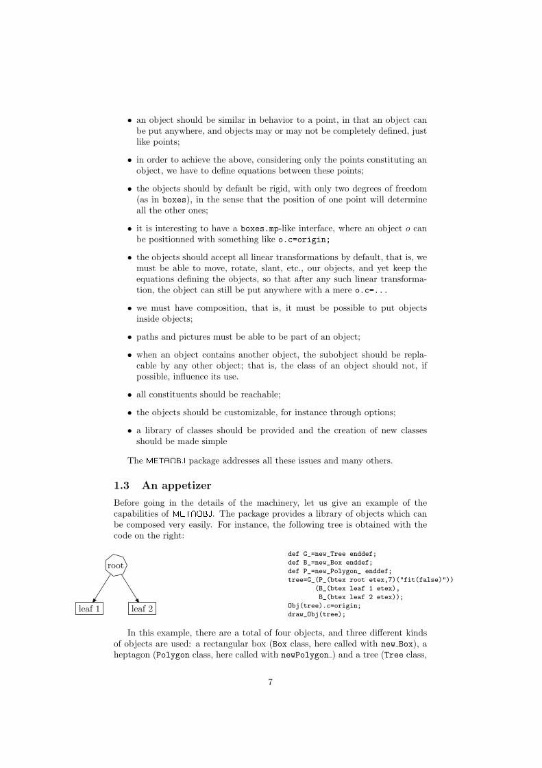
Before going in the details of the machinery, let us give an example of thecapabilities of metaobj. The package provides a library of objects which canbe composed very easily. For instance, the following tree is obtained with thecode on the right:
leaf 1 leaf 2
rootdef G_=new_Tree enddef;
def B_=new_Box enddef;
def P_=new_Polygon_ enddef;
tree=G_(P_(btex root etex,7)("fit(false)"))
(B_(btex leaf 1 etex),
B_(btex leaf 2 etex));
Obj(tree).c=origin;
draw_Obj(tree);
In this example, there are a total of four objects, and three different kindsof objects are used: a rectangular box (Box class, here called with new Box), aheptagon (Polygon class, here called with newPolygon ) and a tree (Tree class,
7
called with new Tree). We have defined a few shortcuts (G_, B_ and P_) andthe tree was built recursively.
new Box, newPolygon (the fact that this one has a trailing _ and not theothers will be explained later) and new Tree are “constructors.” The new Boxconstructor takes a picture and frames it. The new Tree constructor takes aroot object and a list of leaves. In this case, we added an option to the rootnode in order to have a regular heptagon. The default is to have these objectsfit the picture, and this is the case with the boxes. They appear as rectangles,not squares.
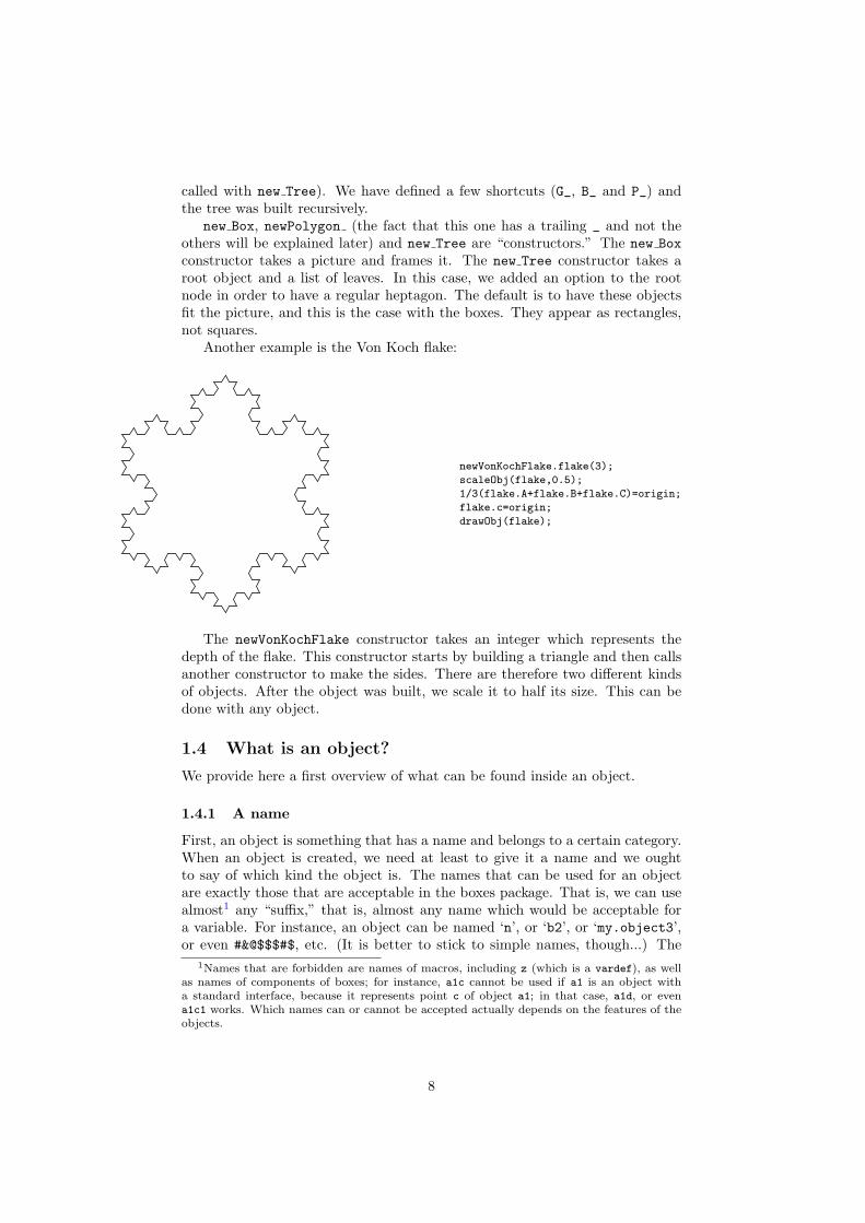
Another example is the Von Koch flake:
newVonKochFlake.flake(3);
scaleObj(flake,0.5);
1/3(flake.A+flake.B+flake.C)=origin;
flake.c=origin;
drawObj(flake);
The newVonKochFlake constructor takes an integer which represents thedepth of the flake. This constructor starts by building a triangle and then callsanother constructor to make the sides. There are therefore two different kindsof objects. After the object was built, we scale it to half its size. This can bedone with any object.
1.4 What is an object?
We provide here a first overview of what can be found inside an object.
1.4.1 A name
First, an object is something that has a name and belongs to a certain category.When an object is created, we need at least to give it a name and we oughtto say of which kind the object is. The names that can be used for an objectare exactly those that are acceptable in the boxes package. That is, we can usealmost1 any “suffix,” that is, almost any name which would be acceptable fora variable. For instance, an object can be named ‘n’, or ‘b2’, or ‘my.object3’,or even #&@$$$#$, etc. (It is better to stick to simple names, though...) The
1Names that are forbidden are names of macros, including z (which is a vardef), as wellas names of components of boxes; for instance, a1c cannot be used if a1 is an object witha standard interface, because it represents point c of object a1; in that case, a1d, or evena1c1 works. Which names can or cannot be accepted actually depends on the features of theobjects.
8
precise rules for suffixes are given in the metafontbook [9]. The name of anobject is used to access its components, as it is done in boxes.
1.4.2 Points
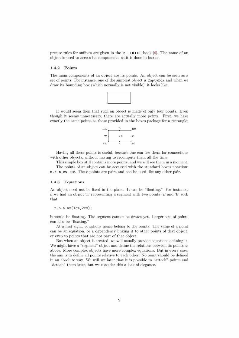
The main components of an object are its points. An object can be seen as aset of points. For instance, one of the simplest object is EmptyBox and when wedraw its bounding box (which normally is not visible), it looks like:
It would seem then that such an object is made of only four points. Eventhough it seems unnecessary, there are actually more points. First, we haveexactly the same points as those provided in the boxes package for a rectangle:
n
s
w e
nenw
sesw
c
Having all these points is useful, because one can use them for connectionswith other objects, without having to recompute them all the time.
This simple box still contains more points, and we will see them in a moment.The points of an object can be accessed with the standard boxes notation:
n.c, n.sw, etc. These points are pairs and can be used like any other pair.
1.4.3 Equations
An object need not be fixed in the plane. It can be “floating.” For instance,if we had an object ‘n’ representing a segment with two points ‘a’ and ‘b’ suchthat
n.b-n.a=(1cm,2cm);
it would be floating. The segment cannot be drawn yet. Larger sets of pointscan also be “floating.”
At a first sight, equations hence belong to the points. The value of a pointcan be an equation, or a dependency linking it to other points of that object,or even to points that are not part of that object.
But when an object is created, we will usually provide equations defining it.We might have a “segment” object and define the relations between its points asabove. More complex objects have more complex equations. But in every case,the aim is to define all points relative to each other. No point should be definedin an absolute way. We will see later that it is possible to “attach” points and“detach” them later, but we consider this a lack of elegance.
9
1.4.4 Pictures
An object can naturally contain pictures. The boxes package provides twofunctions, boxit and circleit, which frame pictures. However, there is a bigdifference between points and pictures: a point can be floating, a picture cannot. A picture is always at some place and an equation will not move it. Youcan assign it to another place, but not just hope it will move alone. The boxespackage always puts the pictures at the origin, and so do we. In order to give thefeeling of “floatness,” we will have a floating point corresponding to the locationof the picture, and everytime we need to draw the picture, we can merely moveit to its location.
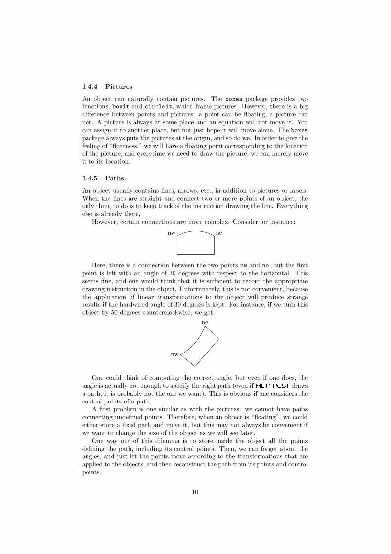
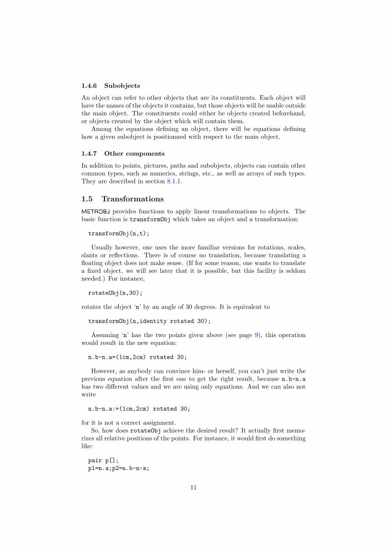
1.4.5 Paths
An object usually contains lines, arrows, etc., in addition to pictures or labels.When the lines are straight and connect two or more points of an object, theonly thing to do is to keep track of the instruction drawing the line. Everythingelse is already there.
However, certain connections are more complex. Consider for instance:
nw ne
Here, there is a connection between the two points nw and ne, but the firstpoint is left with an angle of 30 degrees with respect to the horizontal. Thisseems fine, and one would think that it is sufficient to record the appropriatedrawing instruction in the object. Unfortunately, this is not convenient, becausethe application of linear transformations to the object will produce strangeresults if the hardwired angle of 30 degrees is kept. For instance, if we turn thisobject by 50 degrees counterclockwise, we get:
nw
ne
One could think of computing the correct angle, but even if one does, theangle is actually not enough to specify the right path (even if metapost drawsa path, it is probably not the one we want). This is obvious if one considers thecontrol points of a path.
A first problem is one similar as with the pictures: we cannot have pathsconnecting undefined points. Therefore, when an object is “floating”, we couldeither store a fixed path and move it, but this may not always be convenient ifwe want to change the size of the object as we will see later.
One way out of this dilemma is to store inside the object all the pointsdefining the path, including its control points. Then, we can forget about theangles, and just let the points move according to the transformations that areapplied to the objects, and then reconstruct the path from its points and controlpoints.
10
1.4.6 Subobjects
An object can refer to other objects that are its constituents. Each object willhave the names of the objects it contains, but those objects will be usable outsidethe main object. The constituents could either be objects created beforehand,or objects created by the object which will contain them.
Among the equations defining an object, there will be equations defininghow a given subobject is positionned with respect to the main object.
1.4.7 Other components
In addition to points, pictures, paths and subobjects, objects can contain othercommon types, such as numerics, strings, etc., as well as arrays of such types.They are described in section 8.1.1.
1.5 Transformations
metaobj provides functions to apply linear transformations to objects. Thebasic function is transformObj which takes an object and a transformation:
transformObj(n,t);
Usually however, one uses the more familiar versions for rotations, scales,slants or reflections. There is of course no translation, because translating afloating object does not make sense. (If for some reason, one wants to translatea fixed object, we will see later that it is possible, but this facility is seldomneeded.) For instance,
rotateObj(n,30);
rotates the object ‘n’ by an angle of 30 degrees. It is equivalent to
transformObj(n,identity rotated 30);
Assuming ‘n’ has the two points given above (see page 9), this operationwould result in the new equation:
n.b-n.a=(1cm,2cm) rotated 30;
However, as anybody can convince him- or herself, you can’t just write theprevious equation after the first one to get the right result, because n.b-n.ahas two different values and we are using only equations. And we can also notwrite
n.b-n.a:=(1cm,2cm) rotated 30;
for it is not a correct assignment.So, how does rotateObj achieve the desired result? It actually first memo-
rizes all relative positions of the points. For instance, it would first do somethinglike:
pair p[];p1=n.a;p2=n.b-n-a;
11

then, it would “refresh” ‘n.a’ and ‘n.b.’ metapost makes it possible to refreshvariables using the whatever construct. whatever is a new yet undefined andunnamed numerical variable. It is unnamed because whatever is not the nameof a variable, but it expands into a variable. Basically, we now refresh thevariables with:
n.a:=whatever;n.b:=whatever;
Then, it is possible to achieve the result by merely saying:
n.b-n.a=(p2-p1) rotated 30;
It is along this scheme that all linear transformations are applied on floatingobjects. Of course, we might have positionned the object at a fixed location,and then done assignments, and finally untied the object, but this would’nt havebeen simpler.
2 A first object
2.1 A segment
We are now ready to create our first object! We will start with the ‘Segment’object. This object will contain two points, ‘a’ and ‘b’, and they will be locatedas in the initial example.
vardef newSegment@#=assignObj(@#,"Segment");ObjPoint a,b;ObjCode "@#b-@#a=(1cm,2cm)";
enddef;
The definition of the segment is pretty straightforward. Everytime we wantto create such a segment, we write something like:
newSegment.s;
meaning that ‘s’ is a new object of class ‘Segment.’ The @# is the definitionrepresents the name of the object.
newSegment is the constructor of the Segment class and all constructors havea name like new〈class〉, though this is only a metaobj convention.
The first instruction of the class, assignObj(@#,"Segment"), memorizesthat the object belongs to the Segment class and does various other initializa-tions.
Points are declared with ObjPoint. This instruction defines @#a and @#b aspairs, but it also does more, as we will see later.
The last instruction declares the equation of the segment. This equation isgiven as a string because it makes it easier to store it for later use. ObjCodenot only applies the equations, it also memorizes them. Several equations canbe given as a list of strings where the name of the object is always representedby @#. (This is done for convenience and we might have represented the object
12
in the string by something else, even though @# can be used elsewhere in theconstructor.)
When an object is created, we can display all its points (as well as otherinformations that we do not describe here) with
showObj s;
This produces:
s.a=(xpart s.b-28.34645,ypart s.b-56.6929)s.b=(xpart s.b,ypart s.b)
As you can see, ‘s.a’ is defined with respect to ‘s.b’. Only one point isunknown.
If we write
s.a=origin;
we get:
s.a=(0,0)s.b=(28.34645,56.6929)
Now, we can apply a rotation:
rotateObj(s,30);
and we have:
s.a=(xpart s.a,ypart s.a)s.b=(xpart s.a-3.79764,ypart s.a+63.27086)
Notice that the object is now no longer attached. This is a choice we made,because you usually seldom want to rotate an object around a point and keepit there. You want to rotate an object and build something with it. The finallocation of an object will then depend on the other objects, and even if you canfix one object, you will not be able to do so with all objects. However, one couldstill write a small function doing a rotation and fixing a given point. This is leftas a trivial exercise.
When we are done with the transformations of the object, we want to drawit. We can of course write
draw s.a--s.b;
but for complex objects, it would become very cumbersome. So, whenever anobject is defined, one also defines a drawing function. In this case, it is verysimple:
def drawSegment(suffix n)=draw n.a--n.b;
enddef;
The initial segment is drawn with
13

drawSegment(s);
and this produces
It is also possible to write
drawObj(s);
and drawObj will call drawSegment. It is actually a good idea to always usedrawObj, because it makes a program easier to maintain. If you wanted to defineanother kind of segment, such as:
vardef newLongSegment@#=assignObj(@#,"LongSegment");ObjPoint a,b;ObjCode "@#b-@#a=2*(1cm,2cm)";
enddef;
you could just replace
newSegment.s;
by
newLongSegment.s;
and there would be no need to change anything else. Of course, in this case,drawSegment and drawLongSegment are probably identical, but usually, this isnot so.
2.2 Connecting two objects
Let us now create two new objects, each being a triangle:
vardef newMyTriangle@#=assignObj(@#,"MyTriangle");ObjPoint a,b,c;ObjCode "@#b-@#a=(2cm,0cm)",
"@#c-@#b=(@#b-@#a) rotated 120";enddef;
def drawMyTriangle(suffix n_)=draw n_.a--n_.b--n_.c--n_.a;
enddef;
We create two of them and we rotate the second one by 180 degrees:
14

newMyTriangle.t1;newMyTriangle.t2;rotateObj(t2,180);t1.a=origin;t2.a-t1.a=(4cm,1cm);drawObj(t1,t2);
This produces
a
a
The second triangle was positionned with respect to the first one. Eventhough we first positionned t1, we could have written
t2.a-t1.a=(4cm,1cm);t1.a=origin;
and would have obtained the same result.Before any of these two equations are given, we have two floating objects.
If we write t2.a-t1.a=(4cm,1cm);, the two objects behave like one object.However, the bond can be broken if needed, using the untieObj function. Forinstance, if we want to detach the second triangle, to rotate it 20 degrees more,and to place it a bit further to the right and up, we can do it with:
newMyTriangle.t1;newMyTriangle.t2;rotateObj(t2,180);t2.a-t1.a=(4cm,1cm);t1.a=origin;drawObj(t1,t2);untieObj(t2);rotateObj(t2,20);t2.a-t1.a=(7cm,2cm);drawObj(t2);
and the result is
a
a
a
15
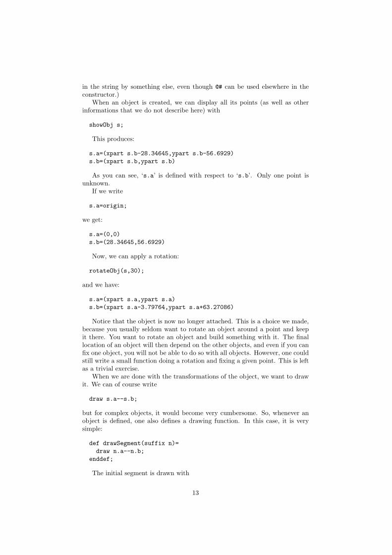
The second triangle appears twice because we have drawn it at its firstposition and at its second position.
This feature can be convenient when it is necessary to use a same componentin several places in a figure. It is also possible to define several objects, or evento clone an existing object. We could have written:
duplicateObj(t3,t2);rotateObj(t3,20);t3.a-t1.a=(7cm,2cm);drawObj(t3);
and the result would still had been the same, because the duplication implicitelyunties an object.
It is important to realize that if one wants to have two identical drawings attwo different places, it is either necessary to draw an object at a first positionand then move it, or have two different objects. But a given object can’t belocated at more than one place at a given time.
The previous example showed how to create several objects and to tie themtogether. But something like t3.a-t1.a=(7cm,2cm) can be accepted only whenat least one of the two objects is floating. Otherwise, there will be an error, mostlikely about an inconsistent equation, because you are trying to move somethingthat can’t be moved by a mere equation. In this case, untying or duplicatingare options to consider.
Once a number of objects are at precise locations, they can be drawn, usingtheir draw functions through drawObj, or by additional draw instructions. Forinstance, if one wants to connect point ‘b’ of the first triangle with point ‘b’ ofthe second triangle, it is sufficient to write:
draw t1.b--t2.b;
giving:
2.3 Creating an object containing objects
Let us consider the previous drawing and assume we somehow need two copiesof it, one being rotated by 90 degrees. This looks more tricky, because what wereally have are three objects and we do not have a means to move them in awhole. We could of course rotate each object, but then they would have to beplaced again at the right positions. This is rather cumbersome! The solution isto create a new object containing the three previous ones. One trivial way is towrite:
16

vardef newThreeTriangles@#=assignObj(@#,"ThreeTriangles");newMyTriangle.t1;newMyTriangle.t2;rotateObj(t2,180);duplicateObj(t3,t2);rotateObj(t3,20);ObjCode "t2.a-t1.a=(4cm,1cm)",
"t3.a-t1.a=(7cm,2cm)";enddef;
def drawThreeTriangles(suffix n)=drawObj(t1,t2,t3);drawarrow t1.b--t2.b;
enddef;
newThreeTriangles.tt;t1.a=origin;drawObj(tt);
This does indeed produce the expected drawing, but there are problemswith what we have done. The objects t1, t2, and t3 are not really marked assubobjects of tt and it won’t be possible to rotate tt. The object tt is virtuallyempty. It contains nothing. As a general rule, all objects should contain at leastone point. All the objects provided in the standard library have at least thecardinal points, which are useful to make use of the object in other contexts.
A better construction could be the following, where we add one point (c),and three subobjects:
vardef newThreeTriangles@#=assignObj(@#,"ThreeTriangles");ObjPoint c;newMyTriangle.t1;newMyTriangle.t2;rotateObj(t2,180);duplicateObj(t3,t2);rotateObj(t3,20);SubObject(suba,t1);SubObject(subb,t2);SubObject(subc,t3);ObjCode "obj(@#subb).a-obj(@#suba).a=(4cm,1cm)",
"obj(@#subc).a-obj(@#suba).a=(7cm,2cm)";StandardTies;
enddef;
The three subobjects are here called suba, subb, and subc. The SubObjectfunction marks an object as a subobject of the current object. In the equations,subobjects are shown with constructions like obj(@#suba). The last line ofthe constructor is the command StandardTies. This command memorizes theconnection between one point of the object (hence the need to have at least
17

one point) and a point of each subobject. It indicates how a subobject must betransformed when a transformation is applied to the object. Usually, the sametransformation is applied to both, but the user could provide his or her ownversion of StandardTies and achieve other effects.
With the previous definition, we can apply various transformations to theobject. However, if we want to make a copy, we must use duplicateObj. Wecan’t just call the constructor twice, like in:
newThreeTriangles.tt1;newThreeTriangles.tt2;
The reason is that each call tries to define the three objects t1, t2, and t3.But all the constructors only work if the object to define is currently undefined.This can be enforced with clearObj and one should therefore write2:
newThreeTriangles.tt1;clearObj t;newThreeTriangles.tt2;
The previous procedure is of course not acceptable, because it means onehas to know what is inside the object. A solution is to create fresh nameswithin the newThreeTriangles function. We can do that with the functionnewobjstring . This function returns a string representing a new object name.It constructs the string using a prefix that should not be used by the user. (Thisprefix can be changed by the user if needed, but it is his or her responsibilityto ensure that it does not conflict with other variables.) In order to access theobject corresponding to the string, one uses the obj function.
vardef newThreeTriangles@#=assignObj(@#,"ThreeTriangles");ObjPoint c;save sa,sb,sc;string sa,sb,sc;sa=newobjstring_;sb=newobjstring_;sc=newobjstring_;newMyTriangle.obj(sa);newMyTriangle.obj(sb);rotateObj(obj(sb),180);duplicateObj(obj(sc),obj(sb));rotateObj(obj(sc),20);SubObject(suba,obj(sa));SubObject(subb,obj(sb));SubObject(subc,obj(sc));ObjCode "obj(@#subb).a-obj(@#suba).a=(4cm,1cm)",
"obj(@#subc).a-obj(@#suba).a=(7cm,2cm)";StandardTies;
enddef;2The clearObj function can currently only be applied to isolated objects (which are not
part of arrays) or arrays, but not to individual objects in an array. t1, t2 and t3 are threeobjects in the t[] array and they are all undefined by the clearObj t call.
18
With the current definition, the constructor can be used several times, andwe can also duplicate the objects that were created, apply transformations, etc.
An alternative to the previous definition can be a parameterized definition,where the three objects are passed to the constructors as parameters. In thiscase, the objects must have been created beforehand. The definition is now:
vardef newThreeTriangles@#(suffix sa,sb,sc)=assignObj(@#,"ThreeTriangles");ObjPoint c;SubObject(suba,sa);SubObject(subb,sb);SubObject(subc,sc);ObjCode "obj(@#subb).a-obj(@#suba).a=(4cm,1cm)",
"obj(@#subc).a-obj(@#suba).a=(7cm,2cm)";StandardTies;
enddef;
This shows that objects are normally manipulated as suffixes. However, wewill see later that there is a special way to use numbers for objects when theobjects are “streamlined.”
The newThreeTriangles constructor is called with:
newMyTriangle.t1;newMyTriangle.t2;rotateObj(t2,180);duplicateObj(t3,t2);rotateObj(t3,20);newThreeTriangles.tta(t1,t2,t3);
The constructor newThreeTriangles can be called several times, with thesame objects. That means actually that the subobjects are shared between twoobjects. So, whenever changes are made to one object, it will result in changesfor the other object. This may or may not be the desired behavior. If one wishesto have two independent objects, one should either use different parametersin the constructors, or merely duplicate an object with duplicateObj. Thisfunction makes a deep copy of an object.
If we want now a rotated copy of the three triangles by 90 degrees, we cansimply write:
duplicateObj(ttb,tta);rotateObj(ttb,90);obj(tta.suba).a=origin;obj(ttb.suba).a=origin+(10cm,-2cm);drawObj(tta,ttb);
The result is shown here:
19

The previous coding is still unsatisfactory, in the way we have to access sub-object points such as obj(tta.suba).a. This is so because our group of threetriangles does not have a point with significance besides those of the subobjects.The ‘c’ point is not used (except internally when memorizing equations) andremains undefined. What we could do is to decide that the ‘c’ point is one ofthe three triangle’s points. In order to say that ‘c’ is the point ‘a’ of the firsttriangle, it is sufficient to add the string "obj(@#suba).a=@#c" to the equationsof newThreeTriangles:
ObjCode "obj(@#subb).a-obj(@#suba).a=(4cm,1cm)","obj(@#subc).a-obj(@#suba).a=(7cm,2cm)","obj(@#suba).a=@#c";
Then, the objects tta and ttb can be simply positionned with:
tta.c=origin;ttb.c=origin+(10cm,-2cm);
This is about the simplest we can get.
We now have a complex construction, with two objects tta and ttb, eachbeing made of three subobjects. Each of these eight objects are accessible inisolation. They all have names. The three triangles of the first object are t1,t2, and t3. The big objects are tta and ttb. And the three other triangleshave names that were generated automatically at the time of the duplication. Itis possible to get these names, but we can also reach these objects logically. Forinstance, the second triangle of ttb is the object obj(ttb.subb). If we desireit, we can draw this object by calling drawObj(obj(ttb.subb)). This showsthat it is better to use drawObj instead of drawMyTriangle, even though thelatter will eventually be called.
All the objects are accessible and so are the points of these objects. We canconnect point ‘a’ of subobject ‘subb’ of object ‘tta’ to point ‘c’ of subobject‘suba’ of object ‘ttb’ by writing
20
draw obj(tta.subb).a--obj(ttb.suba).c;
More complex structures can be built and we will still be able to access thecomplete internal structure.
3 Interfaces and reusability
As long as objects are built in isolation, for a unique use, there are few con-straints on their construction. But when one builds a library of objects, thereare important issues which must be addressed. The main issue is the reusabil-ity. It is desirable to have objects that can be used like black boxes. When anobject contains a subobject, this subobject should be replaceable by any otherobject meeting certain standards. This will make the construction of objectsmuch easier since an object will not have to know the inside of the objects itcontains.
3.1 Standard points
In order to achieve such a modularity, we take as a convention that all objectshave a minimal set of points that can be used from the outside. Two objectsmay have different points, but they will at least have this minimal set. Thisminimal set is called the “standard interface” of an object. It is what an objectof the library can assume of a subobject. This of course is only a conventionof our library and the objects we have created so far didn’t have this standardinterface, and they were anyway quite usable.
The purpose of the standard interface is to help plug in the object in a varietyof contexts. It won’t work for all contexts and sometimes it will be necessary touse more information than the mere standard interface, but such an interfaceprovides already quite interesting facilities.
The standard interface should also serve to define the bounding box of anobject.
We therefore decided to take as the standard interface points all the pointsdefined in boxes such as those provided by boxes.mp. All the objects of ourlibrary will contain the points n, s, e, w, ne, nw, se, sw and c. We stress thatthis is only a convention and that one can define objects that do not have thatinterface, but then the user may have more work to do when plugging objectsinto one another.
However, this is not the whole story! The previous nine points are actuallyonly the “external standard interface.” There is also an “internal standardinterface” made of the nine points in, is, ie, iw, ine, inw, ise, isw and ic.Initially, the internal interface is identical to the external one, that is, for eachobject, points n and in, points s and is, etc., are at the same location. Butcertain operations to the objects can break these identities as we will see later.
The external interface is what should be used from outside the object. Theinternal interface is what should be used from the inside. This distinction doesprove quite useful in certain cases.
In order to declare an object with a standard interface, it is sufficient towrite
StandardInterface;
21

as part of the constructor, right after the assignObj call.
3.2 Standard equations
The standard points are initially connected according to equations that arecalled the standard equations. These equations are divided in the pure standardequations and the inner standard equations. The metaobj package defines thepure standard equations with:
def PureStandardEquations=("@#se-@#sw=@#ne-@#nw;" & % parallelogram equation"xpart(@#se-@#ne)=0;" &"ypart(@#se-@#sw)=0;" &"@#n=.5[@#ne,@#nw];" & % North"@#s=.5[@#se,@#sw];" & % South"@#e=.5[@#ne,@#se];" & % East"@#w=.5[@#nw,@#sw];" & % West"@#c=.5[@#n,@#s];" ) % Center
enddef;
These equations are given as string constants so that they can be used withinthe ObjCode section of a constructor. They define a rectangular shape.
The standard internal equations are defined with:
def StandardInnerEquations=("@#ine=@#ne;@#inw=@#nw;@#isw=@#sw;@#ise=@#se;" &"@#in=@#n;@#is=@#s;@#ie=@#e;@#iw=@#w;@#ic=@#c;")
enddef;
Finally, all the standard equations are defined by:
def StandardEquations=(PureStandardEquations & StandardInnerEquations)
enddef;
In order to define the newThreeTriangles constructor with both a standardinterface and standard equations, we can write:
vardef newThreeTriangles@#(suffix sa,sb,sc)=assignObj(@#,"ThreeTriangles");StandardInterface;SubObject(suba,sa);SubObject(subb,sb);SubObject(subc,sc);ObjCode StandardEquations,
"obj(@#subb).a-obj(@#suba).a=(4cm,1cm)","obj(@#subc).a-obj(@#suba).a=(7cm,2cm)","obj(@#suba).a=@#c";
StandardTies;enddef;
22
Here, the previous explicit definition of point ‘c’ is now part of the standardinterface and this is now the ‘c’ to which refers the last equation.
It is however not sufficient to declare the standard interface and the standardequations. They still have to be defined. Having undefined points is not aproblem per se, but because these points may be used by the context of theobject. It is therefore the responsibility of the constructor to attach the pointsso that all points and subobjects are tied together. However, the attachmentmust only be relative. If it were not, we would have the (light) burden to haveto unattach the object after it is created.
The definition of the points involves additional equations, which tie theinterface to the subobjects. The new equations must take care not to violatethe standard equations. That means that the standard equations must be arectangle.
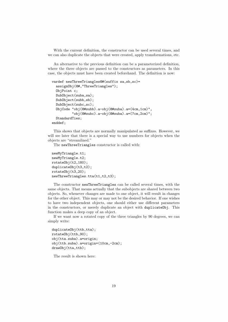
One possible solution is to add "@#ne=obj(@#subc).a". This is sufficient todefine all the points of the interface, because of the constraints of the standardequations. We can now draw the interface (by adding a suitable draw functionto the drawThreeTriangles definition):
nenw
sesw
c
This may not be what we want for a bounding box, but it is what we askedfor! Point c is the middle of [sw,ne] as a consequence of the standard equations.It is the responsibility of the constructor to define the standard interface sothat the content of the object is inside. In certain cases, one may want to haveobjects protrude or take only some of the space to achieve special effects. Thecurrent interface will have the effect that the object will behave, at least withthe standard library, as if it were larger than it really is.
We can get a better result with different equations:
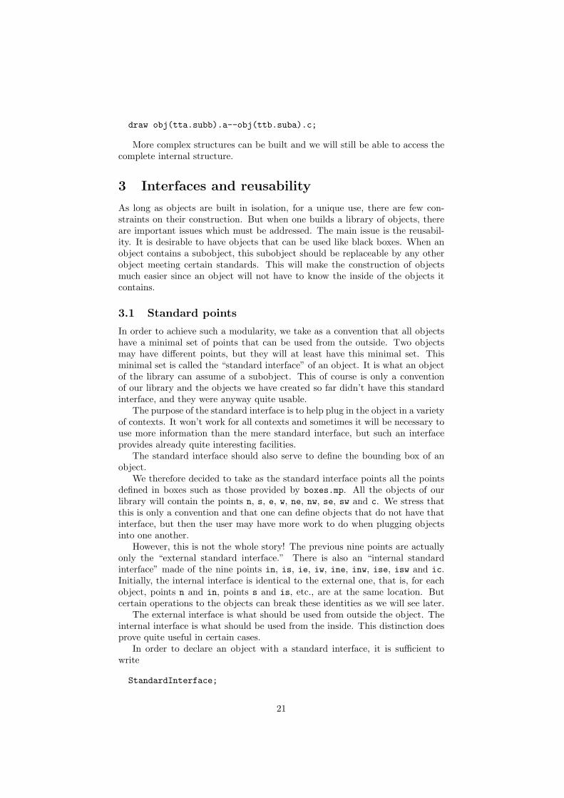
ObjCode StandardEquations,"obj(@#subb).a-obj(@#suba).a=(4cm,1cm)","obj(@#subc).a-obj(@#suba).a=(7cm,2cm)","@#sw=(xpart(obj(@#suba).a),ypart(obj(@#subb).c))","@#ne=obj(@#subc).a";
23
nenw
sesw
Here we defined the ‘sw’ point as having the same xpart as point ‘a’ ofsubobject suba and the same ypart as point ‘c’ of subobject subb.
Incidentally, we would have obtained the same result with the functionrebindVisibleObj, even with an inappropriate definition of the cardinal points.This function takes an object and moves the (outside) cardinal points so thatthey encloses the visible part tightly. However, in order for this to work, thecardinal points must be attached to the object.
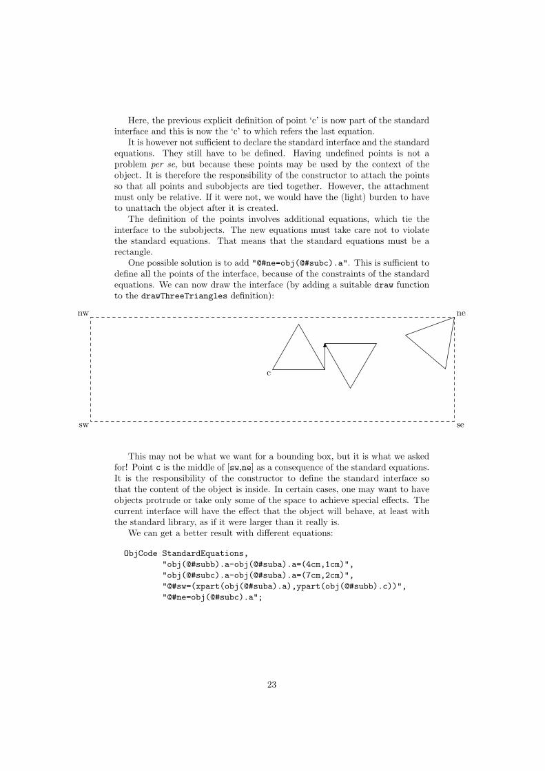
If we now apply transformations to the object, the interface will follow thetransformations. The previous object rotated clockwise by 30 degrees produces:
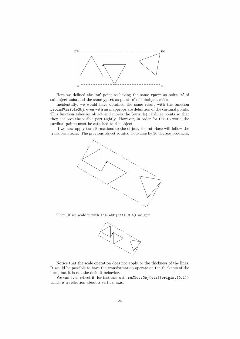
Then, if we scale it with scaleObj(tta,0.5) we get:
Notice that the scale operation does not apply to the thickness of the lines.It would be possible to have the transformation operate on the thickness of thelines, but it is not the default behavior.
We can even reflect it, for instance with reflectObj(tta)(origin,(0,1))which is a reflection about a vertical axis:
24
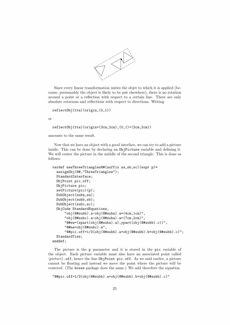
Since every linear transformation unties the objet to which it is applied (be-cause, presumably the object is likely to be put elsewhere), there is no rotationaround a point or a reflection with respect to a certain line. There are onlyabsolute rotations and reflections with respect to directions. Writing
reflectObj(tta)(origin,(0,1))
or
reflectObj(tta)(origin+(3cm,2cm),(0,1)+(3cm,2cm))
amounts to the same result.
Now that we have an object with a good interface, we can try to add a pictureinside. This can be done by declaring an ObjPicture variable and defining it.We will center the picture in the middle of the second triangle. This is done asfollows:
vardef newThreeTriangles@#(suffix sa,sb,sc)(expr p)=assignObj(@#,"ThreeTriangles");StandardInterface;ObjPoint pic.off;ObjPicture pic;setPicture(pic)(p);SubObject(suba,sa);SubObject(subb,sb);SubObject(subc,sc);ObjCode StandardEquations,
"obj(@#subb).a-obj(@#suba).a=(4cm,1cm)","obj(@#subc).a-obj(@#suba).a=(7cm,2cm)","@#sw=(xpart(obj(@#suba).a),ypart(obj(@#subb).c))","@#ne=obj(@#subc).a","@#pic.off=1/3(obj(@#subb).a+obj(@#subb).b+obj(@#subb).c)";
StandardTies;enddef;
The picture is the p parameter and it is stored in the pic variable ofthe object. Each picture variable must also have an associated point called〈picture〉.off, hence the line ObjPoint pic.off. As we said earlier, a picturecannot be floating and instead we move the point where the picture will becentered. (The boxes package does the same.) We add therefore the equation
"@#pic.off=1/3(obj(@#subb).a+obj(@#subb).b+obj(@#subb).c)"
25
which defines the center of the picture as the center of the second triangle.In order to draw the picture, the drawThreeTriangles function must be
augmented with a call to drawPicture. This function automatically uses thelocation of the picture.
def drawThreeTriangles(suffix n)=drawObj(obj(n.suba),obj(n.subb),obj(n.subc));drawarrow obj(n.suba).b--obj(n.subb).b;drawPicture.n(pic);
enddef;
And since drawPicture uses the picturecolor option to find out which colorit should use, we have to specify a default picture color for the ThreeTrianglesclass:
setObjectDefaultOption("ThreeTriangles")("picturecolor")(black);
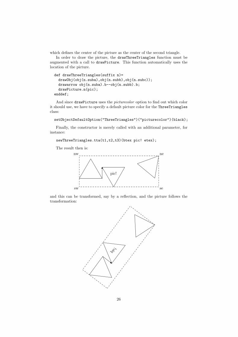
Finally, the constructor is merely called with an additional parameter, forinstance:
newThreeTriangles.tta(t1,t2,t3)(btex pic! etex);
The result then is:
pic!
nenw
sesw
and this can be transformed, say by a reflection, and the picture follows thetransformation:
pic!
26
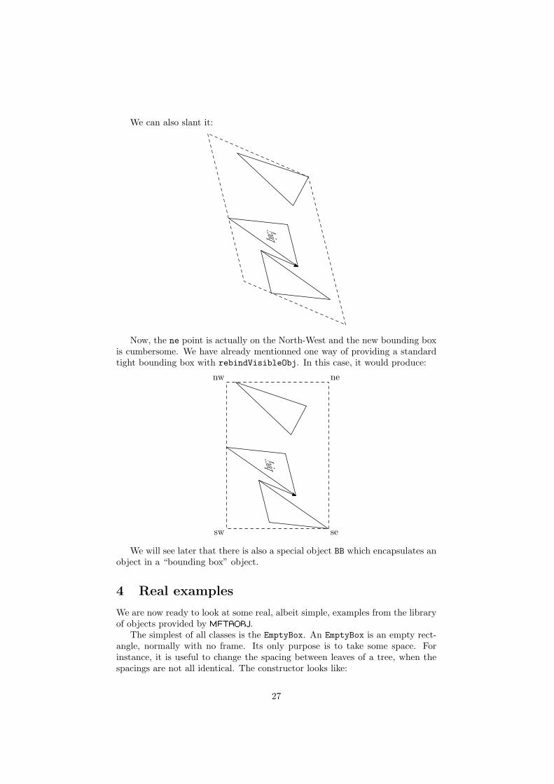
We can also slant it:
pic!
Now, the ne point is actually on the North-West and the new bounding boxis cumbersome. We have already mentionned one way of providing a standardtight bounding box with rebindVisibleObj. In this case, it would produce:
pic!
nenw
sesw
We will see later that there is also a special object BB which encapsulates anobject in a “bounding box” object.
4 Real examples
We are now ready to look at some real, albeit simple, examples from the libraryof objects provided by metaobj.
The simplest of all classes is the EmptyBox. An EmptyBox is an empty rect-angle, normally with no frame. Its only purpose is to take some space. Forinstance, it is useful to change the spacing between leaves of a tree, when thespacings are not all identical. The constructor looks like:
27
vardef newEmptyBox@#(expr dx,dy) text options=ExecuteOptions(options);assignObj(@#,"EmptyBox");StandardInterface;ObjCode StandardEquations,
"@#ise-@#isw=(" & decimal dx & ",0)","@#ine-@#ise=(0," & decimal dy & ")";
enddef;
It is called with two dimensions, which are the sides of the rectangle. Itshould be noticed that the values of dx and dy can be negative and this makesup for some special effects as we will see later.
This function also exhibits some features related to the options mecha-nism. Every constructor can have options modifying its behavior. The optionsare given as the last parameters of the constructor and are used in a call toExecuteOptions. Each object decides which option it honors and how. TheEmptyBox doesn’t have many options, but it is still possible to draw its framewith a different thickness or even to fill the box. Therefore, the drawEmptyBoxfunction actually is (with slight simplifications):
def drawEmptyBox(suffix n)=if show_empty_boxes:drawFramedOrFilledObject_(n);
fi;drawMemorizedPaths_(n);
enddef;
This function is simple: depending on the global variable show_empty_boxes(often used for debugging), the empty boxes are shown or not. If they are shown,they are either filled or merely drawn. The drawFramedOrFilledObject takescare of the various cases. If they are filled, they are filled with a color that canbe given as an option.
If the object is filled, the “bounding path” of the object is used, and it isgiven by the function BpathEmptyBox. Like drawObj which calls drawEmptyBox,BpathObj calls BpathEmptyBox. Each object must declare its “bounding path”function. For EmptyBox, we have
def BpathEmptyBox(suffix n)=StandardBpath(n) enddef;
The standard bouding path provided by StandardBpath is merely the pathn.inw--n.isw--n.ise--n.ine--cycle. This path uses the inner interface sothat the drawing of the object does not depend on artificial changes to itsbounding box.
A more elaborate class is the RecursiveBox. An object of this class con-tains either no object or one object, and in this case, the subobject is also aRecursiveBox. As can be seen, a constructor can call another constructor. Weneed to give a fresh name to the subobject and we call newobjstring . Andwe also call StandardTies in order to ensure that the whole structure can bemanipulated easily. This function memorizes a connection between the mainobject and the subobjects.
28

vardef newRecursiveBox@#(expr n) text options=
ExecuteOptions(@#)(options);
assignObj(@#,"RecursiveBox");
StandardInterface;
% we create a subobject only when |n|>0
if n>0:
% we find a name for the subobject:
SubObject(sub,obj(newobjstring_));
% and we continue to create the hierarchy:
newRecursiveBox.obj(@#sub)(n-1);
rotateObj(obj(@#sub),OptionValue@#("rotangle"));
% the equations are slightly adapted from |newBB|:
ObjCode StandardEquations,
"save lftmost,rtmost,topmost,botmost;",
"string lftmost,rtmost,topmost,botmost;",
"lftmost=find_lft_most.obj(@#sub);",
"rtmost =find_rt_most.obj(@#sub);",
"topmost=find_top_most.obj(@#sub);",
"botmost=find_bot_most.obj(@#sub);",
"xpart(@#inw)=xpart(obj(@#sub).obj(lftmost));",
"xpart(@#ine)=xpart(obj(@#sub).obj(rtmost));",
"ypart(@#inw)=ypart(obj(@#sub).obj(topmost));",
"ypart(@#isw)=ypart(obj(@#sub).obj(botmost));";
else:
ObjCode StandardEquations,
"@#ise-@#isw=(" & decimal (OptionValue@#("dx")) & ",0)",
"@#ine-@#ise=(0," & decimal (OptionValue@#("dy")) & ")";
fi;
StandardTies;
enddef;
Figure 1: RecursiveBox constructor
The equations are not the same whether there is a subobject or not. If thereis no subobject, the object is actually quite similar to an empty box. When thereis a subobject, this one is created with newRecursiveBox. It is then rotatedwith rotateObj. The equations handle the positionning of the subobject withrespect to the main object. First, the bounds of the subobject are computed.Since the subobject has been rotated, we can’t be sure that the nw point isreally the left and top most point. The extreme values are computed with thefind lft most, find rt most, find top most and find bot most functions.They are used to specify the constraints on the main object’s inner interface.
One should also notice that equations that are too long to fit on a line canbe split like strings are split. One should not write two strings separated by acomma, because internally a semicolon is added at the end of each string.
def BpathRecursiveBox(suffix n)=StandardBpath(n) enddef;
The drawRecursiveBox function is interesting, because it shows that onecan check if a given object has some features. Here, we call drawObj on asubobject only when there is a subobject. We could of course have resorted toother ways, like storing the depth of the object within the object. This couldhave been done with an ObjNumeric declaration.
def drawRecursiveBox(suffix n)=
29
drawFramedOrFilledObject_(n);if known n.sub:drawObj(obj(n.sub));
fi;drawMemorizedPaths_(n);
enddef;
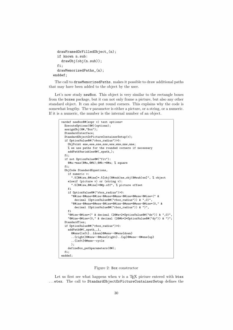
The call to drawMemorizedPaths makes it possible to draw additional pathsthat may have been added to the object by the user.
Let’s now study newBox. This object is very similar to the rectangle boxesfrom the boxes package, but it can not only frame a picture, but also any otherstandard object. It can also put round corners. This explains why the code issomewhat lengthy. The v parameter is either a picture, or a string, or a numeric.If it is a numeric, the number is the internal number of an object.
vardef newBox@#(expr v) text options=
ExecuteOptions(@#)(options);
assignObj(@#,"Box");
StandardInterface;
StandardObjectOrPictureContainerSetup(v);
if OptionValue@#("rbox_radius")>0:
ObjPoint ene,ese,sse,ssw,wsw,wnw,nnw,nne;
% we use paths for the rounded corners if necessary
addPathVariables@#(_spath_);
fi;
if not OptionValue@#("fit"):
@#a:=max(@#a,@#b);@#b:=@#a; % square
fi;
ObjCode StandardEquations,
if numeric v:
".5[@#isw,@#ine]=.5[obj(@#sub)ne,obj(@#sub)sw]", % object
elseif (picture v) or (string v):
".5[@#isw,@#ine]=@#p.off", % picture offset
fi
if OptionValue@#("rbox_radius")>0:
"@#ine-@#nne=@#ise-@#sse=@#nnw-@#inw=@#ssw-@#isw=(" &
decimal (OptionValue@#("rbox_radius")) & ",0)",
"@#ine-@#ene=@#ese-@#ise=@#inw-@#wnw=@#wsw-@#isw=(0," &
decimal (OptionValue@#("rbox_radius")) & ")",
fi
"@#ise-@#isw=(" & decimal (2@#a+2*OptionValue@#("dx")) & ",0)",
"@#ine-@#ise=(0," & decimal (2@#b+2*OptionValue@#("dy")) & ")";
StandardTies;
if OptionValue@#("rbox_radius")>0:
addPath@#(_spath_,1,
@#nnw{left}..{down}@#wnw--@#wsw{down}
..{right}@#ssw--@#sse{right}..{up}@#ese--@#ene{up}
..{left}@#nne--cycle
);
defineBox_pathparameters(@#);
fi;
enddef;
Figure 2: Box constructor
Let us first see what happens when v is a TEX picture entered with btex. . . etex. The call to StandardObjectOrPictureContainerSetup defines the
30
picture as a part of the object (with ObjPicture), it defines a point p.offwhich is used in one of the equations, and it computes the half diagonal of theobject as vector stored into (a_,b_).
When v is a string, the text is set in the current font, without calling TEX.When v is an object, this vector is computed too. Afterwards, we work withthis vector, and this simplifies the equations. The constructor then modifies thevector in case the rectangle must not fit. If it fits, its size adapts to the size ofthe object. Otherwise, the rectangle is a square. Therefore, if the fit option isnot set to true, a_ and b_ are defined to be equal to their maximum.
The newBox constructor distinguishes one special case: if the corners arerounded (rbox radius> 0), eight new points are defined with ObjPoint; therounded frame will pass through these eight points; this frame is defined at theend of the constructor with a call to addPath.
All the points are linked through the equations defined with ObjCode. Afirst part of the code defines either the relative position of the contained object,or the picture offset if it is a picture which is boxed. A second part of the codedefines the additional points depending on the values of the options. The lasttwo equations involve two dimensions, dx and dy, which have default values butcan be given different values as options. They represent a clearance betweenthe picture or the object and the frame.
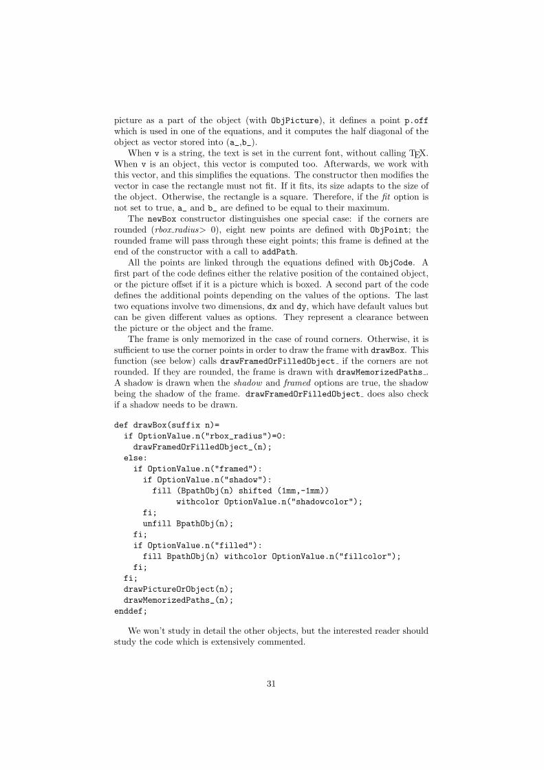
The frame is only memorized in the case of round corners. Otherwise, it issufficient to use the corner points in order to draw the frame with drawBox. Thisfunction (see below) calls drawFramedOrFilledObject if the corners are notrounded. If they are rounded, the frame is drawn with drawMemorizedPaths .A shadow is drawn when the shadow and framed options are true, the shadowbeing the shadow of the frame. drawFramedOrFilledObject does also checkif a shadow needs to be drawn.
def drawBox(suffix n)=if OptionValue.n("rbox_radius")=0:drawFramedOrFilledObject_(n);
else:if OptionValue.n("framed"):if OptionValue.n("shadow"):fill (BpathObj(n) shifted (1mm,-1mm))
withcolor OptionValue.n("shadowcolor");fi;unfill BpathObj(n);
fi;if OptionValue.n("filled"):fill BpathObj(n) withcolor OptionValue.n("fillcolor");
fi;fi;drawPictureOrObject(n);drawMemorizedPaths_(n);
enddef;
We won’t study in detail the other objects, but the interested reader shouldstudy the code which is extensively commented.
31
5 Advanced operations
5.1 Streamlined constructors
There are two ways to build an object with metaobj. The object can bebuilt by calls to the various constructors and all the objects involved can get aname. This forces the user to devise names. Of course, arrays of names can beused in order to overcome this burden. But sometimes, we may wish a more“structural” construction of an object, where an object is built and immediatelyplugged into another one which is built, and so on.
This requires a change in the constructors. For instance, in order to createa box ‘b’, one can write
newBox.b(btex a test box etex);
This is a function call which returns no value. It only modifies the box towhich b refers. Since this call does not return a value, it is not well suited for aplugin. For instance, we can’t write
newBox.b2(newBox.b1(btex an inner box etex));
In order to overcome this problem, we can use a “streamlined” constructorand use “streamlined” constructions. The “streamlined” version of the previous— failed — attempt is
b=new_Box(new_Box(btex an inner box etex));
Here, new Box returns an integer corresponding to a box which was created.new Box can also take a object as parameter when the number of the objectis passed. The outer call to new Box returns a value which must be stored.Then, a special version of drawObj called draw Obj must be used to draw theconstruction:
draw_Obj(b);
This can of course be done only after b has been positionned. This howevercan’t be done by simply writing b.c=..., because b is not the name of anobject. The real object name can be obtained with a call to the Obj function.One should therefore write:
Obj(b).c=...
in order to define point c of the object represented by the integer b.
All the standard objects have a streamlined version. This version was definedwith a call to streamline. Here is the call for the EmptyBox class:
streamline("EmptyBox")("(expr dx,dy)","(dx,dy)");
What this says is that the streamlined version will take two parameterswhich are expressions and will pass them to the non streamlined version. Whencertain arguments are not expressions, for instance if they are lists, the call tostreamline is different. For the Tree class, it is:
32
streamline("Tree")("(expr theroot)(text subtrees)","suffixpar(theroot)suffixlist(subtrees)");
This means that the streamlined version will receive a root number and alist of subtrees numbers. But these parameters can’t be passed like that to thenon-streamlined version. The numbers must be converted into suffixes and thisis what suffixpar and suffixlist do.
In addition to the constructors, several operations have streamlined versions,so that they can operate in a streamlined context. For instance, the streamlinedversion of rotateObj is rotate Obj. In order to create a first box with the text“abc,” to rotate it counterclockwise by 24 degrees and to frame it again, we cansimply write:
b=new_Box(rotate_Obj(new_Box(btex abc etex),24));
If this seems too complex, the user is advised to define shortcuts. This wasdone in one of the first examples, when we showed that trees could be built.
The streamlined versions however are incompatible with the options mech-anism for non-streamlined constructors. Therefore, we provide two streamlinedversions of each constructor: the normal one, and a streamlined version whichsupports options. This version has a trailing _. This explains why the firstpolygon was defined with new Polygon . The second form of streamlined con-structors has a mandatory additional parameter which is a list of options. Thelist can be empty, but the opening and closing parentheses must be there.
In the tree example, the option given to the polygon was "fit(false)",meaning that the polygon must not fit.
5.2 Cloning
Objects can be cloned with duplicateObj, or duplicate Obj which is itsstreamlined version. This creates a deep copy which is completely indepen-dant of the original object. A duplicated object is not attached, whether theoriginal object was attached or not, because most likely the copy will be putelsewhere than the original object.
5.3 Fiddling with the bounding box
The bounding box of an object is its outer interface. It is what is used by othermetaobj functions, and especially those honoring the standard interfaces, inorder to decide how an object is positionned. There are however cases wherethe automatic computation is inadequate. For instance, certain functions onlyfunction appropriately when the bounding boxes are rectangles with horizontaland vertical sides, and with the cardinal points (nw, ne, etc.) located whereone expects them. This, alas, is not always the case when transformations areapplied. There are two major remedies to that:
• an additionnal layer can be added to an object, hiding the idiosyncrasiesof the object and making sure the object “behaves” correctly;
• an object can be coerced to have a normal interface, without the intro-duction of an additional layer.
33

5.3.1 BB: a new bounding box layer
A new layer can be added to an object with the newBB constructor. This is aclass taking an object and enclosing it in a standard interface. The standardinterface tightly encloses the four corners of the object. newBB only looks at thefour corners and there is no guarantee that the “enclosed” object lies entirelyinside the new object interface. Rebinding the object (next section) may bemore appropriate in certain cases.
newBB is similar to rebindObj, but the latter function doesn’t add a layer.
BB options
Option Type Defaultfilled boolean falsefillcolor color blackframed boolean falseframewidth numeric .5bpframecolor color blackframestyle string ""shadow boolean falseshadowcolor color black
5.3.2 Rebinding an object
metaobj provides two ways to rebind an object without adding a layer:
• the rebindObj and its variants move the corner points of an object in sucha way that they are arranged according to a standard initial interface; thepoints are only moved with respect to their former positions, and not withrespect to other components of the object;
– rebindObj(n) is the basic call; it rebinds the object n;– rebindrelativeObj(dyn,dys,dxe,dxw): this function is called by the
rebindObj function (with the four parameters equal to 0) and rebindsand adds shifts in the four directions; dyn is positive when the topcorners must be extended to the top, and negative otherwise; dys ispositive when the bottom corners must be extended to the top, andnegative otherwise; dxe is positive when the right corners must beextended to the right, and negative otherwise; and dxw is positivewhen the left corners must be extended to the right, and negativeotherwise; that way, one can obtain any rectangular bounding box(with horizontal and vertical sides) one may wish;
– extendObjRight.n(wd) specializes rebindrelativeObj and movesthe bounding box of n on the right side so that its width is wd ;
– similarly, extendObjLeft, extendObjUp and extendObjDown adjustthe bounding box on the other sides.
• the rebindVisibleObj also moves the corner points of an object, but ittakes into account all visible parts of an object; this function is useful inorder to ensure that no part of an object protrudes its bounding box; anexample of its use is given in section 7.5.1.
34
5.4 Unattaching an object
When an object is created with a constructor, it is “floating.” For instance,
newBox.a(btex hello! etex);
is a box which is not located at a precise point and an attempt to draw it wouldproduce an error.
Before drawing an object, it must be attached. We could write for instance:
a.c=origin;
Now the object can be drawn, but it can no longer be used at other locationsbecause it is attached. In certain cases, it is useful to be able to unattach anobject and it can be done with untieObj:
untieObj(a);
After this operation, an object can be put elsewhere. The untieObj is usedinternally when paths are added to “floating” objects. In that case, the objectis first fixed, the path is added, and then the object is again untied.
If untieObj is called on an already unattached object, the object is notchanged.
5.5 Options
Many of the objects of the standard metaobj library are parameterized. Forinstance, a Box is parameterized by its content, which is an explicit parameter,but also by other parameters that can be implicit. We call such parameters“options.” An option is therefore an information that can be passed to a con-structor, but which has a default value otherwise. This mechanisme gives us alot of flexibility and avoids providing a long list of parameters that are mostlynot used.
5.5.1 Syntax
The way an option is provided differs according to whether the constructor isused in its normal or streamlined form. When a normal constructor is called,the options are given as lists of strings after the constructor. Each string hasthe syntax "name(value)" where value does not contain quotes. The stringsare comma-separated. Here are a few examples:
newEmptyBox.a(2cm,1cm) "framed(true)";newRandomBox.a(2cm,1cm,2mm,-1mm)"framed(true)", "framewidth(1mm)";
newHBox.c(b,a)"hbsep(1cm)", "framed(true)", "align(center)","dx(5mm)", "dy(5mm)";
The list of options ends with the semi-colon.When a streamlined constructor is used, the same construction cannot be
used, because the semi-colon usually lies beyond the scope of the constructor.
35
Therefore, there are two versions of the streamlined constructors, one with op-tions, and one with no options. For the HBox class, the two constructors arenew_HBox_ (with options) and new_HBox (no options). In addition to the normalparameters of the constructor, the option-streamlined version has an addition-nal parameter which is the list of options. Hence, the three previous exampleswould be written:
new_EmptyBox_(2cm,1cm)("framed(true)")new_RandomBox_(2cm,1cm,2mm,-1mm)
("framed(true)", "framewidth(1mm)")new_HBox_(b,a)("hbsep(1cm)", "framed(true)", "align(center)",
"dx(5mm)", "dy(5mm)")
These streamlined constructors returns numbers and are usually used asparameters to other constructors.
5.5.2 Option types
A given option, such as framed , has a type. The type is always the same fora given option, and it is not possible to have options with the same name, butdifferent types in different objects. For instance, the type of framed is boolean.Its value can be true, false, or some expression returning a boolean. Manyoptions have a numerical type and they usually correspond to some dimensionin an object. In all cases but one, the value between parentheses is of the typethe option awaits. There is one exception, when the type of the option is astring. In this case, quotes are implicitely added to the value between paren-theses. For instance, the align option takes a string as parameter and somehowalign(center) should be understood as align("center"). The standard li-brary reference (section 7) gives the list of all options of all objects, as well astheir type.
Moreover, options can be either local or global. Local and global optionsare used with exactly the same syntax, but in the first case, the option can onlybe used within the constructor of the object, and therefore doesn’t need to bestored inside the object, whereas in the second case, the option value may beused beyond the constructor, for instance when the object is drawn. An optionof a given name is either local or global, but can’t be local to one object andglobal to another.
Finally, each option has a default value. This default value depends onthe class and can be changed by the user with setObjectDefaultOption. Forinstance, the treemode default value for a Tree object is "D" which means thatby default a tree is drawn with the root at the top and the leaves going down.This is declared in metaobj with:
setObjectDefaultOption("Tree")("treemode")("D");
The value can be changed at any time and it will affect all future calls to thenewTree constructor. Of course, the same effect can be obtained by passing anoption such as "treemode(U)" to a constructor, but in the latter case, it needsto be done for all calls to the constructor.
36
5.5.3 Option definition
Options can be defined easily. Here is how the filled and treemode options aredefined:
define_global_boolean_option("filled");define_local_string_option("treemode");
The first is global because the information is used when the object is drawn,and the second is local because it is only used at the time of the object con-struction.
OptionValue.t(v) returns the value of option v of object t. For instance,in order to find out if an object should be filled or not, one could write:
if OptionValue.t("filled"):...
fi;
There are many such examples in the metaobj source code.
5.5.4 Option names
All the options recognized by an object are shown in section 7. In addition tothe options given there, it is possible to use a name option. This option makesit possible to provide an explicit name to an object. This is of course usefulonly in case one uses the streamlined version of a constructor. The name givento an object can then be used later, for instance in connection commands.
5.6 Adding paths to objects
The easiest way to add some line to an object is to add an instruction suchas draw in the function drawing an object. In that case, the line drawn is notreally part of the object, but part a command belonging to the class. However,it is also possible to include lines, and more generally paths, to the structurerepresenting an object.
More precisely, objects can contain one or more path arrays. Each array cancontain several paths and each path is stored as an array of points. This makesit possible to have “floating paths” which is not possible when using the pathtype of metapost.
A path array has a name and must be declared with addPathVariables.This function takes two parameters, the first being an immediate suffix. Thefirst parameter is the object to which the path array is added, and the secondparameter is the name of the array. Currently, two names of arrays have aspecial meaning:
• _spath_ is the array of standard paths of an object; standard paths rep-resent paths that normally come with the object; for instance, in the caseof trees, the node connections from a node to its children are consideredstandard;
• _upath_ is the array of user paths; this array is for paths added by theuser, but which could not be devised automatically.
37
Each path array keeps track of many parameters and options and the ap-propriate structures are defined with addPathVariables. As an example, thenewBox constructor does (@# is the box object):
addPathVariables@#(_spath_);
when there are round corners. In this case, the newBox constructor willmemorize the frame as a path, because it is not a simple path made of straightlines.
The path is then memorized with addPath. newBox does the following:
addPath@#(_spath_,1,@#nnw{left}..{down}@#wnw--@#wsw{down}..{right}@#ssw--@#sse{right}..{up}@#ese--@#ene{up}..{left}@#nne--cycle);
This means that the path @#nnw{left} ... --cycle is stored at index 1 ofthe _spath_ array in the current box object.
In addition to storing the path, various options are also recorded after theaddPath call. For instance, the number of stored paths has to be incremented.
The memorized path is drawn in the drawBox function when the functiondrawMemorizedPaths is called.
Usually, the user does not need to use addPath directly because there arehigher level functions, such as ncline, nccurve, adapted from PSTricks. Thesefunctions take various parameters and feed them into addPath.
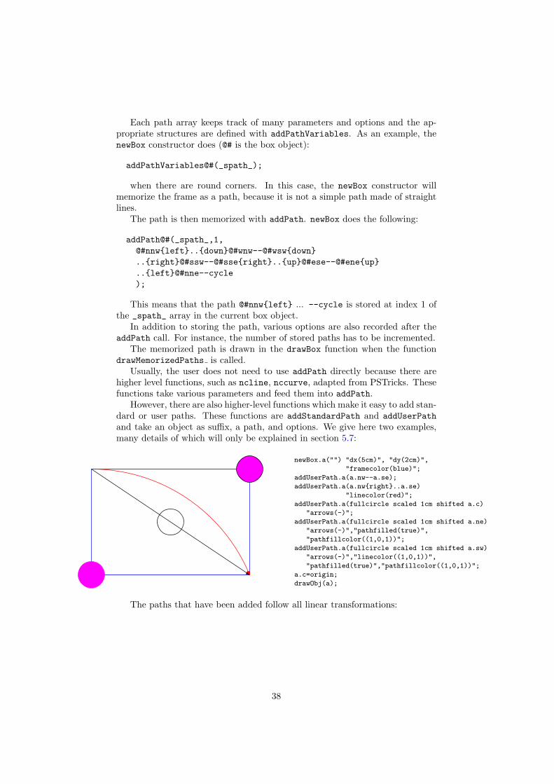
However, there are also higher-level functions which make it easy to add stan-dard or user paths. These functions are addStandardPath and addUserPathand take an object as suffix, a path, and options. We give here two examples,many details of which will only be explained in section 5.7:
newBox.a("") "dx(5cm)", "dy(2cm)",
"framecolor(blue)";
addUserPath.a(a.nw--a.se);
addUserPath.a(a.nw{right}..a.se)
"linecolor(red)";
addUserPath.a(fullcircle scaled 1cm shifted a.c)
"arrows(-)";
addUserPath.a(fullcircle scaled 1cm shifted a.ne)
"arrows(-)","pathfilled(true)",
"pathfillcolor((1,0,1))";
addUserPath.a(fullcircle scaled 1cm shifted a.sw)
"arrows(-)","linecolor((1,0,1))",
"pathfilled(true)","pathfillcolor((1,0,1))";
a.c=origin;
drawObj(a);
The paths that have been added follow all linear transformations:
38
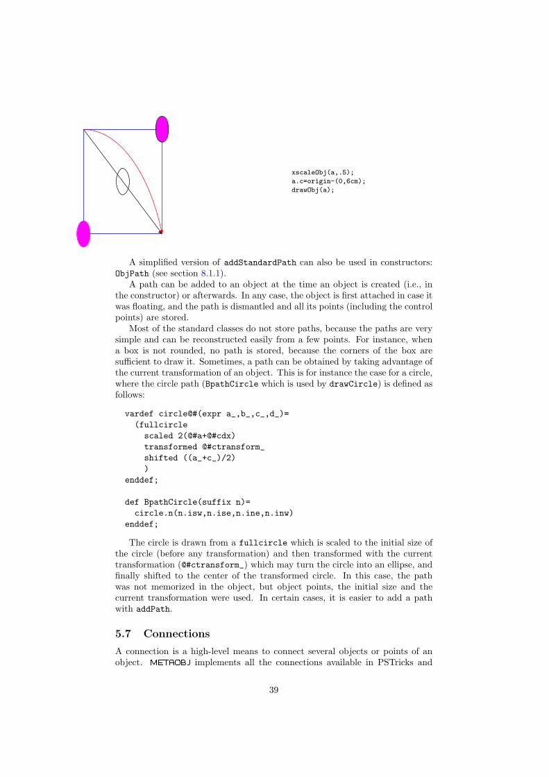
xscaleObj(a,.5);
a.c=origin-(0,6cm);
drawObj(a);
A simplified version of addStandardPath can also be used in constructors:ObjPath (see section 8.1.1).
A path can be added to an object at the time an object is created (i.e., inthe constructor) or afterwards. In any case, the object is first attached in case itwas floating, and the path is dismantled and all its points (including the controlpoints) are stored.
Most of the standard classes do not store paths, because the paths are verysimple and can be reconstructed easily from a few points. For instance, whena box is not rounded, no path is stored, because the corners of the box aresufficient to draw it. Sometimes, a path can be obtained by taking advantage ofthe current transformation of an object. This is for instance the case for a circle,where the circle path (BpathCircle which is used by drawCircle) is defined asfollows:
vardef circle@#(expr a_,b_,c_,d_)=(fullcirclescaled 2(@#a+@#cdx)transformed @#ctransform_shifted ((a_+c_)/2))
enddef;
def BpathCircle(suffix n)=circle.n(n.isw,n.ise,n.ine,n.inw)
enddef;
The circle is drawn from a fullcircle which is scaled to the initial size ofthe circle (before any transformation) and then transformed with the currenttransformation (@#ctransform_) which may turn the circle into an ellipse, andfinally shifted to the center of the transformed circle. In this case, the pathwas not memorized in the object, but object points, the initial size and thecurrent transformation were used. In certain cases, it is easier to add a pathwith addPath.
5.7 Connections
A connection is a high-level means to connect several objects or points of anobject. metaobj implements all the connections available in PSTricks and
39
our description borrows a lot from PSTricks. There is not however an identityof behaviors and sometimes metaobj interprets a parameter in a way differ-ent to the one used by PSTricks, because it suits better the metaobj model.The PSTricks connection commands are \ncline, \nccurve, etc., and meta-obj uses exactly the same names. In addition to these standard connectioncommands, metaobj provides special variants such as tcline and mcline forncline, etc.
All the connection commands except nccircle connect two points or twoobjects. They can therefore take as parameters either objects or points. Pointsmust be given as pair variables. Objects can be given by their name, or by ashortcut given to an object with the name option. If an object is given by itsnumber and not its name, the Obj command can be used to produce the objectname from the object number. For instance, if a and b are objects, we can writeeither ncline(a)(b) or:
an=a;bn=b;ncline(Obj(an))(Obj(bn));
Moreover, a connection is either immediate or deferred. An immediate con-nection is a connection which is not part of an object and is drawn immedi-ately. A deferred connection is a connection which is memorized in an objectand drawn later. The syntax for both cases is the same, except that the ob-ject name, when present, is given as a suffix to the connection command. Forinstance, ncline.A(a)(b) is a deferred connection command connecting theobjects a and b (assuming these are objects) and the connection is memorizedwithin the object A. If we write ncline(a)(b), we get an immediate connectionbetween a and b.
Each of the connection commands has many options. These options make itpossible to change the style of the connection, the thickness of the line, wherethe line starts, etc. The options have types and default values, but the defaultvalues are not bound to a class. The complete set of options is the following:
The types and default values of the options are summarized in table 1.The default values can be changed with setCurveDefaultOption. For in-
stance, the default value for arrows is "drawarrow" and it can be changed to"draw" with:
setCurveDefaultOption("arrows","draw");
Incidentally, we might also have written
setCurveDefaultOption("arrows","-");
because metaobj provides several shortcuts for the kind of arrows. Currentlythe following shortcuts are implemented, but others will probably be added:
Shortcut Full function name- draw-> drawarrow<- rdrawarrow
40
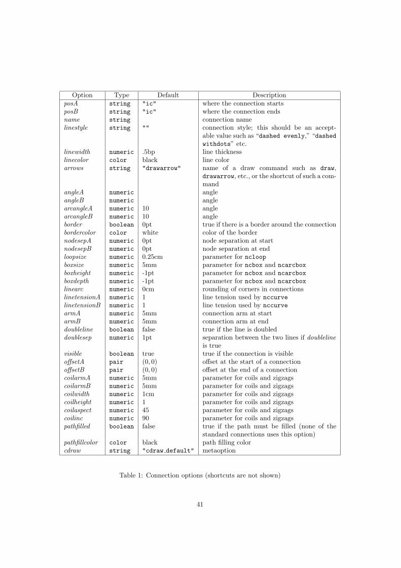
Option Type Default DescriptionposA string "ic" where the connection startsposB string "ic" where the connection endsname string connection namelinestyle string "" connection style; this should be an accept-
able value such as “dashed evenly,” “dashedwithdots” etc.
linewidth numeric .5bp line thicknesslinecolor color black line colorarrows string "drawarrow" name of a draw command such as draw,
drawarrow, etc., or the shortcut of such a com-mand
angleA numeric angleangleB numeric anglearcangleA numeric 10 anglearcangleB numeric 10 angleborder boolean 0pt true if there is a border around the connectionbordercolor color white color of the bordernodesepA numeric 0pt node separation at startnodesepB numeric 0pt node separation at endloopsize numeric 0.25cm parameter for ncloopboxsize numeric 5mm parameter for ncbox and ncarcboxboxheight numeric -1pt parameter for ncbox and ncarcboxboxdepth numeric -1pt parameter for ncbox and ncarcboxlinearc numeric 0cm rounding of corners in connectionslinetensionA numeric 1 line tension used by nccurvelinetensionB numeric 1 line tension used by nccurvearmA numeric 5mm connection arm at startarmB numeric 5mm connection arm at enddoubleline boolean false true if the line is doubleddoublesep numeric 1pt separation between the two lines if doubleline
is truevisible boolean true true if the connection is visibleoffsetA pair (0, 0) offset at the start of a connectionoffsetB pair (0, 0) offset at the end of a connectioncoilarmA numeric 5mm parameter for coils and zigzagscoilarmB numeric 5mm parameter for coils and zigzagscoilwidth numeric 1cm parameter for coils and zigzagscoilheight numeric 1 parameter for coils and zigzagscoilaspect numeric 45 parameter for coils and zigzagscoilinc numeric 90 parameter for coils and zigzagspathfilled boolean false true if the path must be filled (none of the
standard connections uses this option)pathfillcolor color black path filling colorcdraw string "cdraw default" metaoption
Table 1: Connection options (shortcuts are not shown)
41

An unsupported sequence of symbols will be equivalent to the “-” value.The cdraw option defines how the other options are used. This option is
very seldom used and is not described in this manual.Several of the options come in two flavors, one for each end of the connection.
This is for instance the case for posA and posB . In this case, special shortcutsare provided. pos is a shortcut option setting both posA and posB . For instance,
ncline(a)(b) "pos(s)";
is equivalent to
ncline(a)(b) "posA(s)","posB(s)";
These shortcuts can also be used with setCurveDefaultOption and whenpassed to a Tree constructor.
The shortcuts currently supported are pos, coilarm, linetension, offset , arm,angle, arcangle and nodesep.
In all the examples below, the two circled objects are produced with:
newCircle.a(btex start etex);newCircle.b(btex end etex);a.c=origin;b.c-a.c=(3cm,2cm);drawObj(a,b);
Some of the descriptions borrow from the PSTricks documentation [16].
5.7.1 ncline
ncline is the simplest of all connection commands. It connects either two pointsor two objects by a straight line. If two objects are connected, the line is cutbefore the bounding path of the first object and after the bounding path of thesecond object.
start
end
ncline(a)(b);
If ncline is used to connect two object points (such as a.c and b.c), thebounding paths of the objects are not taken into account:
start
end
ncline(a.c)(b.c);
42
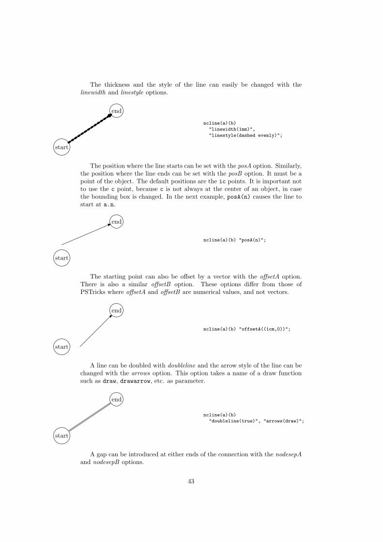
The thickness and the style of the line can easily be changed with thelinewidth and linestyle options.
start
end
ncline(a)(b)
"linewidth(1mm)",
"linestyle(dashed evenly)";
The position where the line starts can be set with the posA option. Similarly,the position where the line ends can be set with the posB option. It must be apoint of the object. The default positions are the ic points. It is important notto use the c point, because c is not always at the center of an object, in casethe bounding box is changed. In the next example, posA(n) causes the line tostart at a.n.
start
end
ncline(a)(b) "posA(n)";
The starting point can also be offset by a vector with the offsetA option.There is also a similar offsetB option. These options differ from those ofPSTricks where offsetA and offsetB are numerical values, and not vectors.
start
end
ncline(a)(b) "offsetA((1cm,0))";
A line can be doubled with doubleline and the arrow style of the line can bechanged with the arrows option. This option takes a name of a draw functionsuch as draw, drawarrow, etc. as parameter.
start
end
ncline(a)(b)
"doubleline(true)", "arrows(draw)";
A gap can be introduced at either ends of the connection with the nodesepAand nodesepB options.
43

start
end
ncline(a)(b)
"nodesepB(10mm)", "arrows(draw)";
5.7.2 nccurve
nccurve draws a Bezier curve between the nodes. The default angles at whichthe curve leaves or reaches the nodes are those obtained when a straight lineconnects the nodes. Hence, without options, nccurve behaves like ncline. Thetwo angles can be changed with the angleA and angleB options.
start
end
nccurve(a)(b) "angleA(0)";
More parameters can be modified, for instance the linecolor , the linewidth,the style with linestyle and the fact that the line is drawn double with doubleline.
start
endnccurve(a)(b)
"angleA(-30)", "angleB(80)",
"linecolor(red)","linewidth(1mm)",
"doubleline(true)",
"linestyle(dashed withdots)";
The tension of the line (in metapost’s sense) can be modified with thelinetensionA and linetensionB options (or with the linetension shortcut). Thisallows a control similar to the one provided with PSTricks’ ncurvA and ncurvBparameters. The default tensions are 1.
start
endnccurve(a)(b)
"angleA(-30)", "angleB(80)",
"linecolor(red)","linewidth(3pt)",
"linestyle(dashed withdots)",
"linetension(2)";
44
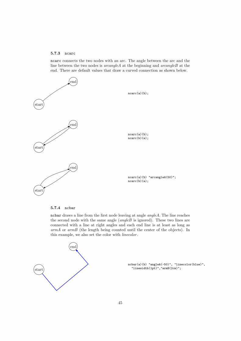
5.7.3 ncarc
ncarc connects the two nodes with an arc. The angle between the arc and theline between the two nodes is arcangleA at the beginning and arcangleB at theend. There are default values that draw a curved connection as shown below.
start
end
ncarc(a)(b);
start
end
ncarc(a)(b);
ncarc(b)(a);
start
end
ncarc(a)(b) "arcangleA(50)";
ncarc(b)(a);
5.7.4 ncbar
ncbar draws a line from the first node leaving at angle angleA. The line reachesthe second node with the same angle (angleB is ignored). These two lines areconnected with a line at right angles and each end line is at least as long asarmA or armB (the length being counted until the center of the objects). Inthis example, we also set the color with linecolor .
start
end
ncbar(a)(b) "angleA(-50)", "linecolor(blue)",
"linewidth(1pt)","armB(2cm)";
45

start
end ncbar(a)(b) "angleA(90)", "linecolor(blue)",
"linewidth(1pt)","armB(2cm)";
5.7.5 ncangle
ncangle usually draws three segments, but in certain cases there are only two.The two extreme segments are at angles defined by the angleA and angleBoptions. The point on the last segment at a distance armB from the node isconnected to node A with a right angle. armA is not taken into account. In thenext example, the first segment is of length 0.
start
end
ncangle(a)(b) "angleA(90)", "angleB(80)",
"linecolor(blue)","linewidth(1pt)","armB(2cm)";
start
end
ncangle(a)(b) "angleA(0)", "angleB(50)",
"linecolor(blue)","linewidth(1pt)",
"armA(3cm)","armB(2cm)";
5.7.6 ncangles
ncangles is similar to ncangle, but the length of arm A (measured from thenode) is fixed by the armA option. Arm A is connected to arm B by twoline segments that meet arm A and each other at right angles. The angle atwhich they join arm B, and the length of the connecting segments, depends onthe positions of the two arms. ncangles generally draws a total of four linesegments.
46

start
end
ncangles(a)(b) "angleA(0)", "angleB(50)",
"linecolor(blue)","linewidth(1pt)",
"armA(3cm)","armB(2cm)";
In the next example, the start of the line is offset by (0, 1cm):
start
end
ncangles(a)(b) "angleA(0)", "angleB(50)",
"linecolor(blue)","linewidth(1pt)",
"armA(3cm)","armB(2cm)","offsetA((0,1cm))";
start
endncangles(a)(b) "angleA(90)", "angleB(50)",
"linecolor(blue)","linewidth(1pt)",
"armA(3cm)","armB(2cm)";
5.7.7 ncdiag
ncdiag draws an arm at each node, joining at angle angleA or angleB , and witha length of armA or armB (from the centers of the nodes). Then the two armsare connected by a straight line, so that the whole line has three line segments.
start
endncdiag(a)(b) "angleA(90)", "angleB(50)",
"linecolor(blue)","linewidth(1pt)",
"armA(3cm)","armB(2cm)";
start
end
ncdiag(a)(b) "angleA(0)", "angleB(90)",
"linecolor(blue)","linewidth(1pt)",
"armA(2cm)","armB(2cm)";
47
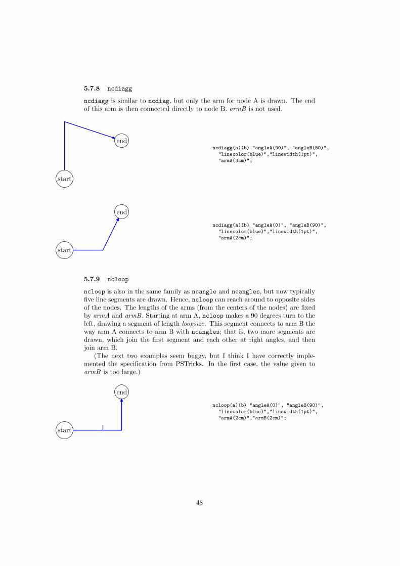
5.7.8 ncdiagg
ncdiagg is similar to ncdiag, but only the arm for node A is drawn. The endof this arm is then connected directly to node B. armB is not used.
start
endncdiagg(a)(b) "angleA(90)", "angleB(50)",
"linecolor(blue)","linewidth(1pt)",
"armA(3cm)";
start
end
ncdiagg(a)(b) "angleA(0)", "angleB(90)",
"linecolor(blue)","linewidth(1pt)",
"armA(2cm)";
5.7.9 ncloop
ncloop is also in the same family as ncangle and ncangles, but now typicallyfive line segments are drawn. Hence, ncloop can reach around to opposite sidesof the nodes. The lengths of the arms (from the centers of the nodes) are fixedby armA and armB . Starting at arm A, ncloop makes a 90 degrees turn to theleft, drawing a segment of length loopsize. This segment connects to arm B theway arm A connects to arm B with ncangles; that is, two more segments aredrawn, which join the first segment and each other at right angles, and thenjoin arm B.
(The next two examples seem buggy, but I think I have correctly imple-mented the specification from PSTricks. In the first case, the value given toarmB is too large.)
start
end
ncloop(a)(b) "angleA(0)", "angleB(90)",
"linecolor(blue)","linewidth(1pt)",
"armA(2cm)","armB(2cm)";
48
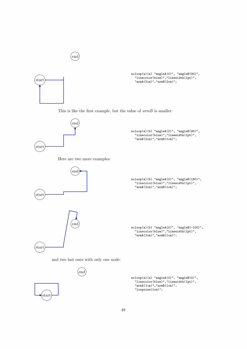
start
end
ncloop(a)(a) "angleA(0)", "angleB(90)",
"linecolor(blue)","linewidth(1pt)",
"armA(2cm)","armB(2cm)";
This is like the first example, but the value of armB is smaller:
start
end
ncloop(a)(b) "angleA(0)", "angleB(90)",
"linecolor(blue)","linewidth(1pt)",
"armA(2cm)","armB(1cm)";
Here are two more examples:
start
end
ncloop(a)(b) "angleA(0)", "angleB(180)",
"linecolor(blue)","linewidth(1pt)",
"armA(2cm)","armB(1cm)";
start
endncloop(a)(b) "angleA(0)", "angleB(-100)",
"linecolor(blue)","linewidth(1pt)",
"armA(2cm)","armB(1cm)";
and two last ones with only one node:
start
endncloop(a)(a) "angleA(0)", "angleB(0)",
"linecolor(blue)","linewidth(1pt)",
"armA(1cm)","armB(1cm)",
"loopsize(1cm)";
49

start
endncloop(a)(a) "angleA(0)", "angleB(0)",
"linecolor(blue)","linewidth(1pt)",
"armA(1cm)","armB(1cm)","loopsize(1cm)",
"offsetA((0,2mm))","offsetB((0,-3mm))";
5.7.10 nccircle
nccircle draws a circle, or part of a circle, that if complete, would pass throughthe center of the node counterclockwise, at an angle of angleA. The angleBoption is not used.
start
end
nccircle(a) "angleA(0)",
"linecolor(blue)","linewidth(1pt)";
5.7.11 ncbox
ncbox and ncarcbox do not connect the nodes with an open curve, but theyenclose the nodes in a box or curved box. The half of the width of the box isboxsize. The dimensions of the box can also be given with the boxheight andboxdepth options. The ends of the boxes extend beyond the nodes by nodesepAand nodesepB . This hence gives two different meanings to these two options.
Two of the sides of the ncbox box are parallel to the line connecting the twonode centers. No angle is taken into account by ncbox.
start
end
ncbox(a)(b)
"linecolor(blue)","linewidth(1pt)",
"nodesepA(1cm)","nodesepB(1cm)";
50

start
endncbox(a)(b)
"linecolor(blue)","linewidth(1pt)",
"nodesepA(1cm)","nodesepB(1cm)",
"boxsize(1cm)";
The corners can be rounded with the linearc option:
start
endncbox(a)(b)
"linecolor(blue)","linewidth(1pt)",
"nodesepA(1cm)","nodesepB(1cm)",
"boxsize(1cm)","linearc(3mm)";
5.7.12 ncarcbox
ncarcbox is similar to ncbox. It encloses the nodes in a curved box that isarcangleA away from the line connecting the two nodes. PSTricks seems tocount that angle clockwise, whereas it is counted counterclockwise in ncarc.We decided for consistency to count the angle counterclockwise in both cases.The arcangleB option is not used.
start
end
ncarcbox(a)(b) "arcangleA(0)",
"linecolor(blue)","linewidth(1pt)",
"nodesepA(1cm)","nodesepB(1cm)";
51
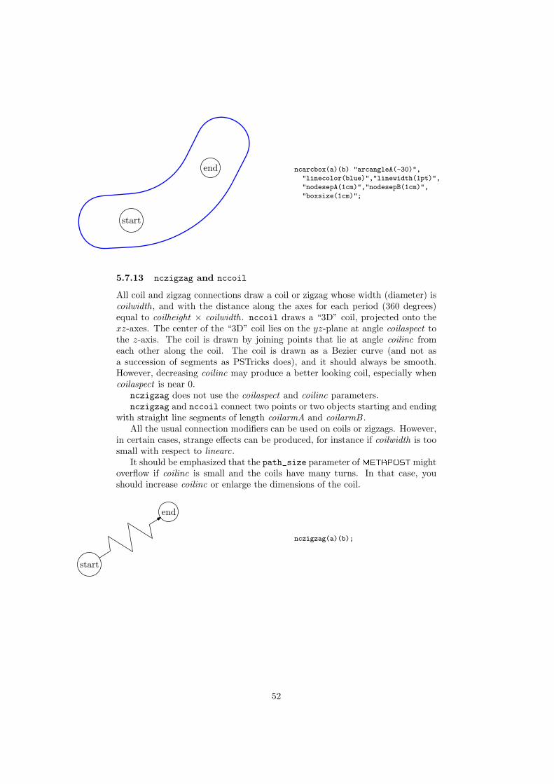
start
end ncarcbox(a)(b) "arcangleA(-30)",
"linecolor(blue)","linewidth(1pt)",
"nodesepA(1cm)","nodesepB(1cm)",
"boxsize(1cm)";
5.7.13 nczigzag and nccoil
All coil and zigzag connections draw a coil or zigzag whose width (diameter) iscoilwidth, and with the distance along the axes for each period (360 degrees)equal to coilheight × coilwidth. nccoil draws a “3D” coil, projected onto thexz-axes. The center of the “3D” coil lies on the yz-plane at angle coilaspect tothe z-axis. The coil is drawn by joining points that lie at angle coilinc fromeach other along the coil. The coil is drawn as a Bezier curve (and not asa succession of segments as PSTricks does), and it should always be smooth.However, decreasing coilinc may produce a better looking coil, especially whencoilaspect is near 0.
nczigzag does not use the coilaspect and coilinc parameters.nczigzag and nccoil connect two points or two objects starting and ending
with straight line segments of length coilarmA and coilarmB .All the usual connection modifiers can be used on coils or zigzags. However,
in certain cases, strange effects can be produced, for instance if coilwidth is toosmall with respect to linearc.
It should be emphasized that the path_size parameter of metapost mightoverflow if coilinc is small and the coils have many turns. In that case, youshould increase coilinc or enlarge the dimensions of the coil.
start
end
nczigzag(a)(b);
52
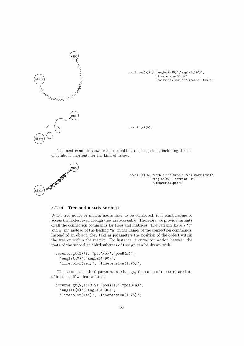
start
end
nczigzag(a)(b) "angleA(-90)","angleB(120)",
"linetension(0.8)",
"coilwidth(2mm)","linearc(.1mm)";
start
end
nccoil(a)(b);
The next example shows various combinations of options, including the useof symbolic shortcuts for the kind of arrow.
start
end
nccoil(a)(b) "doubleline(true)","coilwidth(2mm)",
"angleA(0)", "arrows(-)",
"linewidth(1pt)";
5.7.14 Tree and matrix variants
When tree nodes or matrix nodes have to be connected, it is cumbersome toaccess the nodes, even though they are accessible. Therefore, we provide variantsof all the connection commands for trees and matrices. The variants have a “t”and a “m” instead of the leading “n” in the names of the connection commands.Instead of an object, they take as parameters the position of the object withinthe tree or within the matrix. For instance, a curve connection between theroots of the second an third subtrees of tree gt can be drawn with:
tccurve.gt(2)(3) "posA(e)","posB(n)","angleA(0)","angleB(-90)","linecolor(red)", "linetension(1.75)";
The second and third parameters (after gt, the name of the tree) are listsof integers. If we had written:
tccurve.gt(2,1)(3,2) "posA(e)","posB(n)","angleA(0)","angleB(-90)","linecolor(red)", "linetension(1.75)";
53
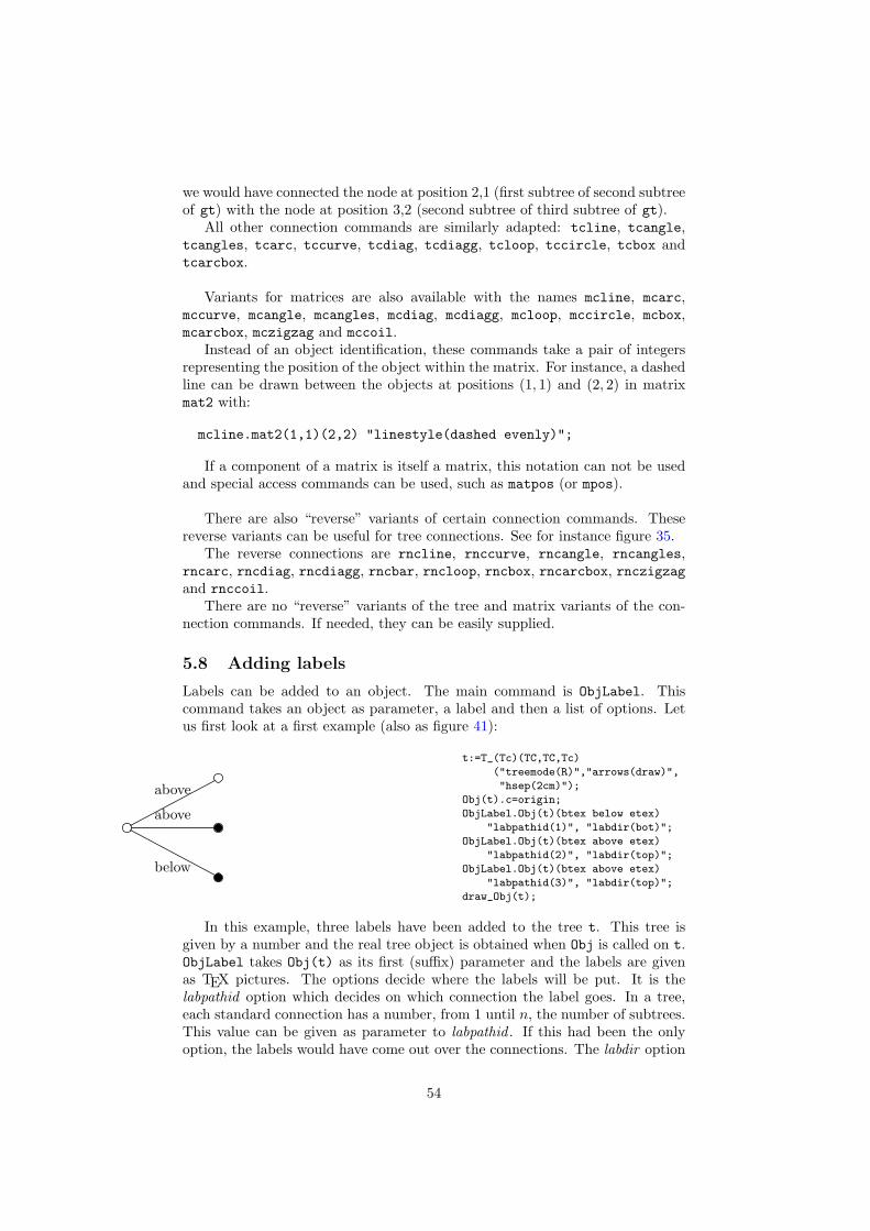
we would have connected the node at position 2,1 (first subtree of second subtreeof gt) with the node at position 3,2 (second subtree of third subtree of gt).
All other connection commands are similarly adapted: tcline, tcangle,tcangles, tcarc, tccurve, tcdiag, tcdiagg, tcloop, tccircle, tcbox andtcarcbox.
Variants for matrices are also available with the names mcline, mcarc,mccurve, mcangle, mcangles, mcdiag, mcdiagg, mcloop, mccircle, mcbox,mcarcbox, mczigzag and mccoil.
Instead of an object identification, these commands take a pair of integersrepresenting the position of the object within the matrix. For instance, a dashedline can be drawn between the objects at positions (1, 1) and (2, 2) in matrixmat2 with:
mcline.mat2(1,1)(2,2) "linestyle(dashed evenly)";
If a component of a matrix is itself a matrix, this notation can not be usedand special access commands can be used, such as matpos (or mpos).
There are also “reverse” variants of certain connection commands. Thesereverse variants can be useful for tree connections. See for instance figure 35.
The reverse connections are rncline, rnccurve, rncangle, rncangles,rncarc, rncdiag, rncdiagg, rncbar, rncloop, rncbox, rncarcbox, rnczigzagand rnccoil.
There are no “reverse” variants of the tree and matrix variants of the con-nection commands. If needed, they can be easily supplied.
5.8 Adding labels
Labels can be added to an object. The main command is ObjLabel. Thiscommand takes an object as parameter, a label and then a list of options. Letus first look at a first example (also as figure 41):
below
above
above
t:=T_(Tc)(TC,TC,Tc)
("treemode(R)","arrows(draw)",
"hsep(2cm)");
Obj(t).c=origin;
ObjLabel.Obj(t)(btex below etex)
"labpathid(1)", "labdir(bot)";
ObjLabel.Obj(t)(btex above etex)
"labpathid(2)", "labdir(top)";
ObjLabel.Obj(t)(btex above etex)
"labpathid(3)", "labdir(top)";
draw_Obj(t);
In this example, three labels have been added to the tree t. This tree isgiven by a number and the real tree object is obtained when Obj is called on t.ObjLabel takes Obj(t) as its first (suffix) parameter and the labels are givenas TEX pictures. The options decide where the labels will be put. It is thelabpathid option which decides on which connection the label goes. In a tree,each standard connection has a number, from 1 until n, the number of subtrees.This value can be given as parameter to labpathid . If this had been the onlyoption, the labels would have come out over the connections. The labdir option
54

is used to shift the label with respect to the normal point where it would havebeen positionned. labdir takes options similar to those taken by the standardmetapost label command.
The table 2 shows the list of all options recognized by the ObjLabel com-mand:
Option name Type Defaultlabpathid numeric /labdir string /labrotate numeric 0labangle numeric /labpos numeric 0.5labshift pair (0, 0)labcolor color blacklaberase boolean falselabpoint string "ic"labcard string /labpathname string /
Table 2: Label options (“/” means that there are no default values)
ObjLabel puts a label either somewhere along a path or somewhere near apoint of an object. Two options help specifying the relevant path:
• labpathid : this option takes a path number as parameter; it is seldomused, except in cases where the path numbers are well known, for instancein the example given previously or in figure 39;
• labpathname: when a path is created (with a connection command suchas ncline, ...), the path can be given a name (with the name option); thisname can be given as parameter to labpathname; examples are given infigure 10.
On a given path, a position can be specified with labpos. This option is anumerical value between 0 and 1. 0 represents the beginning of the path (if thepath starts at the bounding path of an object, this is also the 0 position) and 1the end of the path. The default value is 0.5.
By default, a label is set horizontally, no matter what is the slope of thepath at the label position. The label can be set parallel to the path direction byspecifying the labangle option with the value 0. Other values rotate the labelwith respect to the path tangent.
A label can also be set with respect to an object point with the labpointoption. For instance,
ObjLabel.g(btex hello! etex) "labpoint(po1)";
writes “hello!” over point po1 of object g.A label can also be set in an object, with respect to a cardinal point with the
labcard option. Like labpoint , labcard takes an object point as parameter, butthe label is not put over the point, but beyond the label point, in a direction
55

determined by the line joining the center of the object and the point. Forinstance, in order to put the label (−10, 10. − 10) below (south) of the objectat position (2, 1, 1) of the tree Obj(t), we can write:
ObjLabel.ntreepos(Obj(t))(2,1,1)(btex $(-10,10.-10)$ etex)"labcard(s)";
(ntreepos is a command taking an object and a tree position as parameters,and returning the node at that position.)
There are four additional options which apply in both cases (labels on a pathor next to a point):
• labrotate: with this option, a label can be rotated with respect to itsnormal position;
• labshift : with this option, a label can be shifted, in a way similar to theoffsetA and offsetB connection options;
• labcolor : this option determines the color of the label;
• laberase: this option determines if the label erases what lies beneath it ornot.
6 The object structure
Figures 3, 4, 5 and 6 are the result of showObj on a PTree object called ptre,slightly rearranged and simplified to make it more readable.
An object has a name and all its direct components form a tree of variables,all starting with the object name. There is unfortunately no easy way to traversesuch a tree of variables in metapost, and there are therefore special variableswhich keep track of what is in an object. We call these variables attributes ofan object. The complete list of attributes is given in table 3.
ptre=100
ptre.numericlist_="dx,dy,nst"
ptre.nst=2
ptre.ctransform_=(0,0,1,0,0,1)
Figure 3: Object structure: general data
As shown in the first figure, an object has a number. Here, it is 100. It haspoints, the list of which is given in the string pointlist which is a standardattribute of the object. It has a list of subobject references, the list of which isgiven as a string sublist . Each subobject is actually only given as a string.The subobject is not really part of the object (and as we said earlier, an objectcan be part of several other objects).
The ptre object belongs to the PTree class and it contains four subobjects.Each subobject has a corresponding string: conc (conclusion), subt (subtrees),lr (left rule), rr (right rule). The value of the string was generated automati-cally by newobjstring .
The structure of ptre was obtained with
56

Attribute Type Default Descriptionpointlist string "" list of pointspairlist string "" list of pairs (non movable points)pointarraylist string "" list of arrays of pointssubarraylist string "" list of arrays of subobjectsstringarraylist string "" list of arrays of stringscolorarraylist string "" list of arrays of colorspicturearraylist string "" list of arrays of picturestransformarraylist string "" list of arrays of transformsbooleanarraylist string "" list of arrays of booleansnumericarraylist string "" list of arrays of numericspairarraylist string "" list of arrays of pairs (non movable points)points in arrayslist string "" enumeration of all (movable) points of all ar-
rays (of movable points)picturelist string "" list of picturesnumericlist string "" list of numericssublist string "" list of subobjectssubobjties string array subobj tying equations (1 string/subobject)nsubobjties numeric 0 number of subobjtiescode string "" code of an objectextra code string "" extra code of an objectctransform transform identity current transform of that object
Table 3: Standard attributes of an object
ptre.pointlist_="ne,nw,sw,se,n,s,e,w,c,
ine,inw,isw,ise,in,is,ie,iw,ic,ledge,redge,lstart,lend"
ptre.c=(0,287.17845)
ptre.n=(0,312.73784)
ptre.s=(0,261.61906)
ptre.e=(95.02467,287.17845)
ptre.w=(-95.02467,287.17845)
ptre.ne=(95.02467,312.73784)
ptre.se=(95.02467,261.61906)
ptre.nw=(-95.02467,312.73784)
ptre.sw=(-95.02467,261.61906)
ptre.ic=(0,283.46451)
ptre.in=(0,308.30998)
ptre.is=(0,258.61905)
ptre.ie=(98.02467,283.46451)
ptre.iw=(-98.02469,283.46451)
ptre.ine=(98.02467,308.30998)
ptre.ise=(98.02467,258.61905)
ptre.inw=(-98.02469,308.30998)
ptre.isw=(-98.02469,258.61905)
ptre.ledge=(-72.57094,258.61905)
ptre.redge=(92.90178,258.61905)
ptre.lstart=(-51.91089,292.35118)
ptre.lend=(65.57219,292.35118)
Figure 4: Object structure (cont’d): points
57
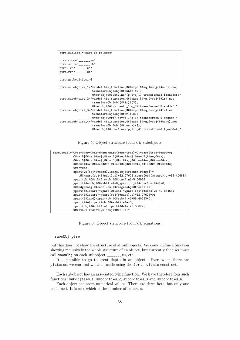
ptre.sublist_="subt,lr,rr,conc"
ptre.conc="_______zu"
ptre.subt="_______zh"
ptre.lr="_______zs"
ptre.rr="_______zt"
ptre.nsubobjties_=4
ptre.subobjties_1="vardef tie_function_@#(expr $)=q_1=obj(@#subt).ne;
transformObj(obj(@#subt))($);
@#ne-obj(@#subt).ne=(p_1-q_1) transformed $;enddef;"
ptre.subobjties_2="vardef tie_function_@#(expr $)=q_2=obj(@#lr).ne;
transformObj(obj(@#lr))($);
@#ne-obj(@#lr).ne=(p_1-q_2) transformed $;enddef;"
ptre.subobjties_3="vardef tie_function_@#(expr $)=q_3=obj(@#rr).ne;
transformObj(obj(@#rr))($);
@#ne-obj(@#rr).ne=(p_1-q_3) transformed $;enddef;"
ptre.subobjties_4="vardef tie_function_@#(expr $)=q_4=obj(@#conc).ne;
transformObj(obj(@#conc))($);
@#ne-obj(@#conc).ne=(p_1-q_4) transformed $;enddef;"
Figure 5: Object structure (cont’d): subobjects
ptre.code_="@#se-@#sw=@#ne-@#nw;xpart(@#se-@#ne)=0;ypart(@#se-@#sw)=0;
@#n=.5[@#ne,@#nw];@#s=.5[@#se,@#sw];@#e=.5[@#ne,@#se];
@#w=.5[@#nw,@#sw];@#c=.5[@#n,@#s];@#ine=@#ne;@#inw=@#nw;
@#isw=@#sw;@#ise=@#se;@#in=@#n;@#is=@#s;@#ie=@#e;@#iw=@#w;
@#ic=@#c;
xpart(.5[obj(@#conc).ledge,obj(@#conc).redge])=
.5[xpart(obj(@#subt).s)-62.07625,xpart(obj(@#subt).s)+55.40683];
ypart(obj(@#subt).s-obj(@#conc).n)=5.66928;
ypart(@#n-obj(@#subt).n)=0;ypart(obj(@#conc).s-@#s)=0;
@#ledge=obj(@#conc).sw;@#redge=obj(@#conc).se;
ypart(@#lstart)=ypart(@#lend)=ypart(obj(@#conc).n)+2.83464;
xpart(@#lstart)=xpart(obj(@#subt).c)-62.07625+0;
xpart(@#lend)=xpart(obj(@#subt).c)+55.40683+0;
xpart(@#e)-xpart(obj(@#subt).e)=+0;
xpart(obj(@#subt).w)-xpart(@#w)=+20.33072;
@#lstart-(rdistl,0)=obj(@#lr).e;"
Figure 6: Object structure (cont’d): equations
showObj ptre;
but this does not show the structure of all subobjects. We could define a functionshowing recursively the whole structure of an object, but currently the user mustcall showObj on each subobject _______zu, etc.
It is possible to go to great depth in an object. Even when there arepictures, we can find what is inside using the for ... within construct.
Each subobject has an associated tying function. We have therefore four suchfunctions, subobjties 1, subobjties 2, subobjties 3 and subobjties 4.
Each object can store numerical values. There are three here, but only oneis defined. It is nst which is the number of subtrees.
58
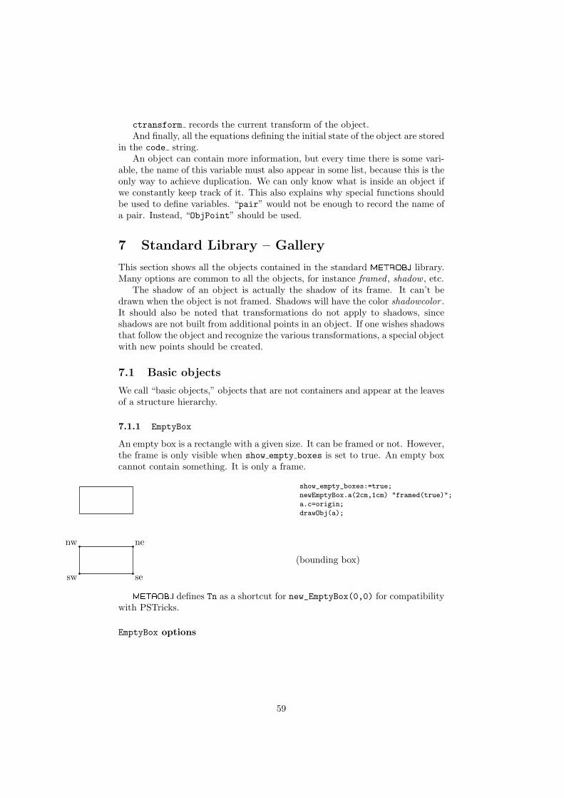
ctransform records the current transform of the object.And finally, all the equations defining the initial state of the object are stored
in the code string.An object can contain more information, but every time there is some vari-
able, the name of this variable must also appear in some list, because this is theonly way to achieve duplication. We can only know what is inside an object ifwe constantly keep track of it. This also explains why special functions shouldbe used to define variables. “pair” would not be enough to record the name ofa pair. Instead, “ObjPoint” should be used.
7 Standard Library – Gallery
This section shows all the objects contained in the standard metaobj library.Many options are common to all the objects, for instance framed , shadow , etc.
The shadow of an object is actually the shadow of its frame. It can’t bedrawn when the object is not framed. Shadows will have the color shadowcolor .It should also be noted that transformations do not apply to shadows, sinceshadows are not built from additional points in an object. If one wishes shadowsthat follow the object and recognize the various transformations, a special objectwith new points should be created.
7.1 Basic objects
We call “basic objects,” objects that are not containers and appear at the leavesof a structure hierarchy.
7.1.1 EmptyBox
An empty box is a rectangle with a given size. It can be framed or not. However,the frame is only visible when show empty boxes is set to true. An empty boxcannot contain something. It is only a frame.
show_empty_boxes:=true;
newEmptyBox.a(2cm,1cm) "framed(true)";
a.c=origin;
drawObj(a);
nw ne
sw se
(bounding box)
metaobj defines Tn as a shortcut for new_EmptyBox(0,0) for compatibilitywith PSTricks.
EmptyBox options
59
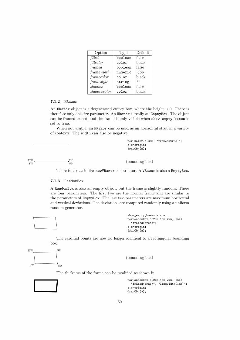
Option Type Defaultfilled boolean falsefillcolor color blackframed boolean falseframewidth numeric .5bpframecolor color blackframestyle string ""shadow boolean falseshadowcolor color black
7.1.2 HRazor
An HRazor object is a degenerated empty box, where the height is 0. There istherefore only one size parameter. An HRazor is really an EmptyBox. The objectcan be framed or not, and the frame is only visible when show_empty_boxes isset to true.
When not visible, an HRazor can be used as an horizontal strut in a varietyof contexts. The width can also be negative.
newHRazor.a(3cm) "framed(true)";
a.c=origin;
drawObj(a);
nw nesw se (bounding box)
There is also a similar newVRazor constructor. A VRazor is also a EmptyBox.
7.1.3 RandomBox
A RandomBox is also an empty object, but the frame is slightly random. Thereare four parameters. The first two are the normal frame and are similar tothe parameters of EmptyBox. The last two parameters are maximum horizontaland vertical deviations. The deviations are computed randomly using a uniformrandom generator.
show_empty_boxes:=true;
newRandomBox.a(2cm,1cm,2mm,-1mm)
"framed(true)";
a.c=origin;
drawObj(a);
The cardinal points are now no longer identical to a rectangular boundingbox.
nw ne
sw se
(bounding box)
The thickness of the frame can be modified as shown in:
newRandomBox.a(2cm,1cm,2mm,-1mm)
"framed(true)", "linewidth(1mm)";
a.c=origin;
drawObj(a);
60

A random box can also be filled, with a given color:
newRandomBox.a(1cm,5mm,2mm,-1mm)
"framed(true)", "filled(true)",
"fillcolor(red)","framewidth(1mm)",
"framecolor(green)";
a.c=origin;
drawObj(a);
RandomBox options
Option Type Defaultfilled boolean falsefillcolor color blackframed boolean trueframewidth numeric .5bpframecolor color blackframestyle string ""shadow boolean falseshadowcolor color black
7.2 Basic containers
All the basic containers take a picture or an object and provide a frame forit. A picture can be one given in the TEX notation (btex...etex) or a pictureobtained in other ways, for instance with the image command of metapost.
7.2.1 Box
Box is the simplest of the containers. It is similar to EmptyBox, but it is acontainer and by default the frame is visible. The size of the box is adapted toits contents.
some textnewBox.a(btex some text etex);
a.c=origin;
drawObj(a);
some textnw ne
sw se(bounding box)
By default, the frame fits the contents. With the fit(false) option, it nolonger does. The frame is then a square.
some text
newBox.a(btex some text etex)
"fit(false)";
a.c=origin;
drawObj(a);
In addition, it is possible to specify horizontal and vertical margins to thecontents with the dx and dy options. If the contents is empty and we want a4mm×4mm square, and if that square must be filled, we can write:
61

newBox.a("") "filled(true)",
"dx(2mm)", "dy(2mm)";
a.c=origin;
drawObj(a);
Round corners can be obtained by specifying a radius. If the radius is toolarge, the clearance (dx and dy) may have to be increased.
This is an ovalbox
newBox.a(btex This is an ovalbox etex)
"rbox_radius(2mm)";
a.c=origin;
drawObj(a);
It is also possible to call the newRBox constructor which is a Box with adefault value of 1mm for rbox radius.
This is a shadowboxnewBox.a(btex This is a shadowbox etex)
"shadow(true)";
a.c=origin;
drawObj(a);
Box options
Option Type Defaultdx numeric 3bpdy numeric 3bpfilled boolean falsefillcolor color blackframed boolean trueshadow boolean falseshadowcolor color blackfit boolean trueframewidth numeric .5bpframecolor color blackframestyle string ""picturecolor color blackrbox radius numeric 0
We might add more options for the shadows in the future.
Box shortcuts metaobj defines a few shortcuts for PSTricks compatibility:
• Tr (p) is equivalent to new_Box_(p)("framed(false)");
• Tf is equivalent to new_Box_("")("filled(true)").
7.2.2 Polygon
The newPolygon constructor builds polygons. Polygons are containers. Thenumber of sides can be specified, and we can decide if the polygon fits thecontents. By default it does. Here is a pentagon:
some textnewPolygon.a(btex some text etex,5);
a.c=origin;
drawObj(a);
62

Some clearance can be added by changing the polymargin option.
some text
newPolygon.a(btex some text etex,5)
"polymargin(3mm)";
a.c=origin;
drawObj(a);
The cardinal points are those of the rectangle bounding the ellipse on whichthe vertices are located. The cardinal points of the previous example are:
some text
nw ne
sw se
(bounding box)
A heptagon which does not fit its contents is:
some text
newPolygon.a(btex some text etex,7)
"fit(false)", "polymargin(3mm)";
a.c=origin;
drawObj(a);
A Polygon can also be rotated. See for instance figure 35.
Polygon options
Option Type Defaultpolymargin numeric 2mmangle numeric 0filled boolean falsefillcolor color blackframed boolean truefit boolean trueframewidth numeric .5bpframecolor color blackpicturecolor color blackframestyle string ""shadow boolean falseshadowcolor color black
7.2.3 Ellipse
The newEllipse constructor builds an ellipse which is a container. The ellipsecan contain text and by default it fits the text. The following ellipse
some textnewEllipse.a(btex some text etex);
a.c=origin;
drawObj(a);
some textnw ne
sw se(bounding box)
63
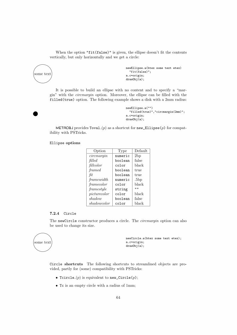
When the option "fit(false)" is given, the ellipse doesn’t fit the contentsvertically, but only horizontally and we get a circle:
some text
newEllipse.a(btex some text etex)
"fit(false)";
a.c=origin;
drawObj(a);
It is possible to build an ellipse with no content and to specify a “mar-gin” with the circmargin option. Moreover, the ellipse can be filled with thefilled(true) option. The following example shows a disk with a 2mm radius:
newEllipse.a("")
"filled(true)","circmargin(2mm)";
a.c=origin;
drawObj(a);
metaobj provides Toval (p) as a shortcut for new_Ellipse(p) for compat-ibility with PSTricks.
Ellipse options
Option Type Defaultcircmargin numeric 2bpfilled boolean falsefillcolor color blackframed boolean truefit boolean trueframewidth numeric .5bpframecolor color blackframestyle string ""picturecolor color blackshadow boolean falseshadowcolor color black
7.2.4 Circle
The newCircle constructor produces a circle. The circmargin option can alsobe used to change its size.
some textnewCircle.a(btex some text etex);
a.c=origin;
drawObj(a);
Circle shortcuts The following shortcuts to streamlined objects are pro-vided, partly for (some) compatibility with PSTricks:
• Tcircle (p) is equivalent to new_Circle(p);
• Tc is an empty circle with a radius of 1mm;
64
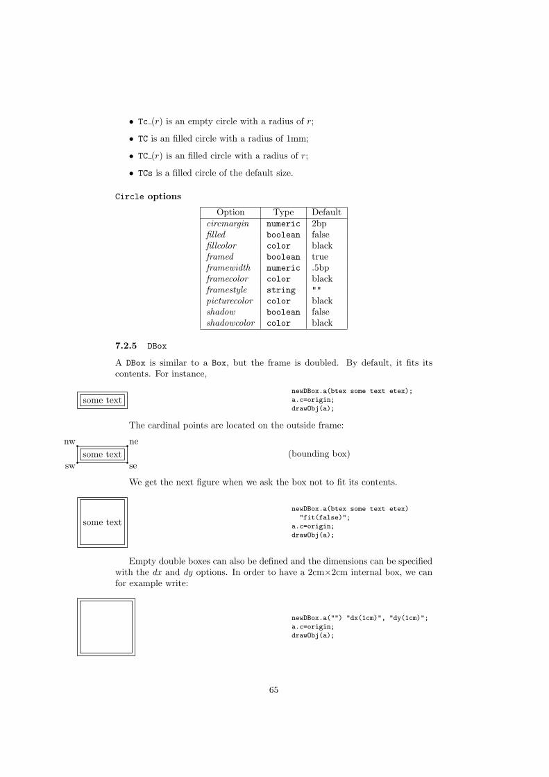
• Tc (r) is an empty circle with a radius of r;
• TC is an filled circle with a radius of 1mm;
• TC (r) is an filled circle with a radius of r;
• TCs is a filled circle of the default size.
Circle options
Option Type Defaultcircmargin numeric 2bpfilled boolean falsefillcolor color blackframed boolean trueframewidth numeric .5bpframecolor color blackframestyle string ""picturecolor color blackshadow boolean falseshadowcolor color black
7.2.5 DBox
A DBox is similar to a Box, but the frame is doubled. By default, it fits itscontents. For instance,
some textnewDBox.a(btex some text etex);
a.c=origin;
drawObj(a);
The cardinal points are located on the outside frame:
some textnw ne
sw se(bounding box)
We get the next figure when we ask the box not to fit its contents.
some text
newDBox.a(btex some text etex)
"fit(false)";
a.c=origin;
drawObj(a);
Empty double boxes can also be defined and the dimensions can be specifiedwith the dx and dy options. In order to have a 2cm×2cm internal box, we canfor example write:
newDBox.a("") "dx(1cm)", "dy(1cm)";
a.c=origin;
drawObj(a);
65
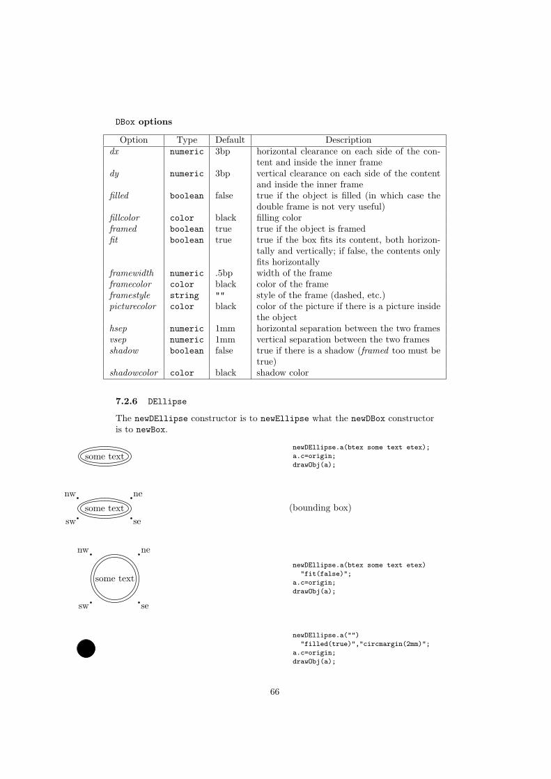
DBox options
Option Type Default Descriptiondx numeric 3bp horizontal clearance on each side of the con-
tent and inside the inner framedy numeric 3bp vertical clearance on each side of the content
and inside the inner framefilled boolean false true if the object is filled (in which case the
double frame is not very useful)fillcolor color black filling colorframed boolean true true if the object is framedfit boolean true true if the box fits its content, both horizon-
tally and vertically; if false, the contents onlyfits horizontally
framewidth numeric .5bp width of the frameframecolor color black color of the frameframestyle string "" style of the frame (dashed, etc.)picturecolor color black color of the picture if there is a picture inside
the objecthsep numeric 1mm horizontal separation between the two framesvsep numeric 1mm vertical separation between the two framesshadow boolean false true if there is a shadow (framed too must be
true)shadowcolor color black shadow color
7.2.6 DEllipse
The newDEllipse constructor is to newEllipse what the newDBox constructoris to newBox.
some textnewDEllipse.a(btex some text etex);
a.c=origin;
drawObj(a);
some text
nw ne
sw se(bounding box)
some text
nw ne
sw se
newDEllipse.a(btex some text etex)
"fit(false)";
a.c=origin;
drawObj(a);
newDEllipse.a("")
"filled(true)","circmargin(2mm)";
a.c=origin;
drawObj(a);
66
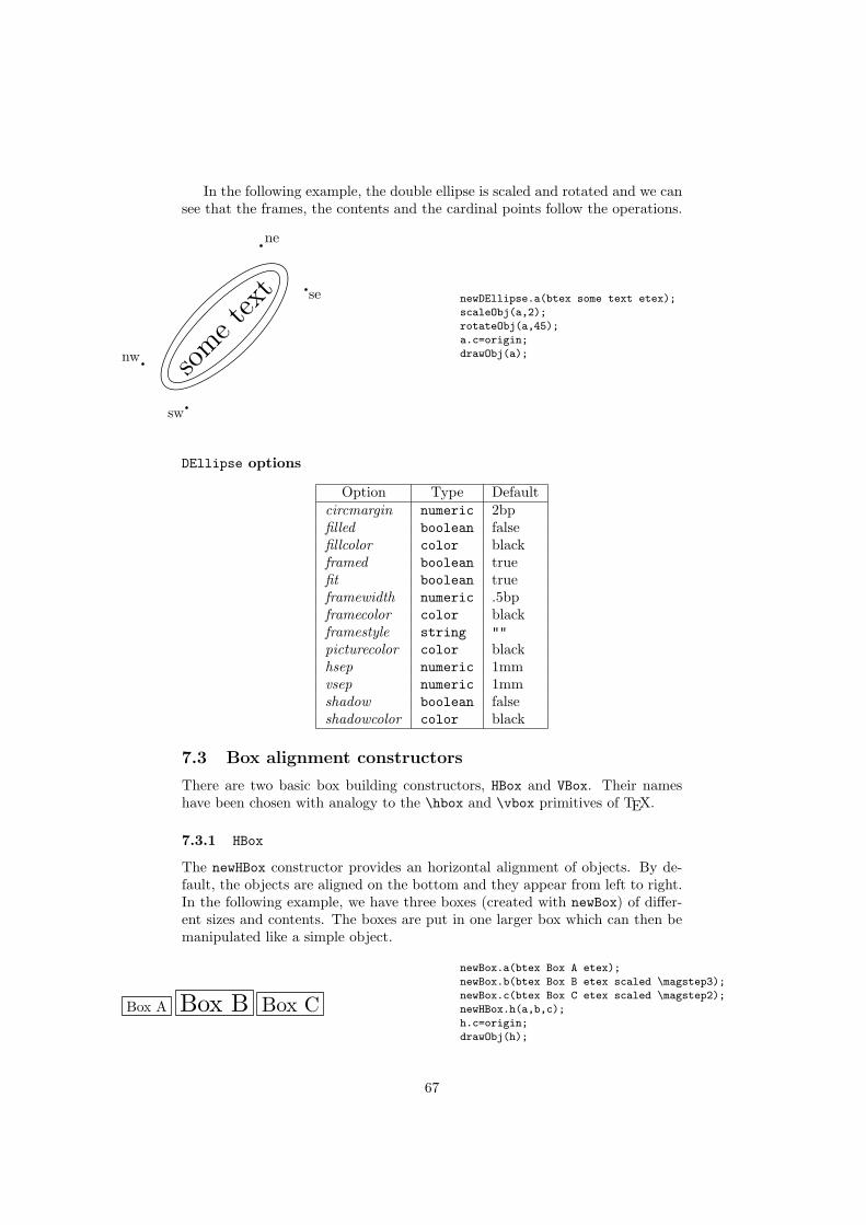
In the following example, the double ellipse is scaled and rotated and we cansee that the frames, the contents and the cardinal points follow the operations.
some tex
t
nw
ne
sw
se newDEllipse.a(btex some text etex);
scaleObj(a,2);
rotateObj(a,45);
a.c=origin;
drawObj(a);
DEllipse options
Option Type Defaultcircmargin numeric 2bpfilled boolean falsefillcolor color blackframed boolean truefit boolean trueframewidth numeric .5bpframecolor color blackframestyle string ""picturecolor color blackhsep numeric 1mmvsep numeric 1mmshadow boolean falseshadowcolor color black
7.3 Box alignment constructors
There are two basic box building constructors, HBox and VBox. Their nameshave been chosen with analogy to the \hbox and \vbox primitives of TEX.
7.3.1 HBox
The newHBox constructor provides an horizontal alignment of objects. By de-fault, the objects are aligned on the bottom and they appear from left to right.In the following example, we have three boxes (created with newBox) of differ-ent sizes and contents. The boxes are put in one larger box which can then bemanipulated like a simple object.
Box A Box B Box C
newBox.a(btex Box A etex);
newBox.b(btex Box B etex scaled \magstep3);
newBox.c(btex Box C etex scaled \magstep2);
newHBox.h(a,b,c);
h.c=origin;
drawObj(h);
67

The cardinal points show the bounding box of the HBox. They are notcompulsory on an object. In the next example, they happen to coincide withthe bottom left and right corners of two boxes, but that is only because the boxesare aligned on the bottom, and because the component objects are rectangularboxes.
Box A Box B Box Cnw ne
sw se(bounding box)
In order to change the alignment, the align option can be given, with eitherbot, top, or center. Here is an alignment at the top, with the same objects:
Box A Box B Box C
newBox.a(btex Box A etex);
newBox.b(btex Box B etex scaled \magstep3);
newBox.c(btex Box C etex scaled \magstep2);
newHBox.h(a,b,c) "align(top)";
h.c=origin;
drawObj(h);
The next example shows objects that are centered vertically:
Box A Box B Box C
newBox.a(btex Box A etex);
newBox.b(btex Box B etex scaled \magstep3);
newBox.c(btex Box C etex scaled \magstep2);
newHBox.h(a,b,c) "align(center)";
h.c=origin;
drawObj(h);
There is a default horizontal separation between objects, but it can bechanged with the hbsep option:
Box A Box B Box C
newBox.a(btex Box A etex);
newBox.b(btex Box B etex scaled \magstep3);
newBox.c(btex Box C etex scaled \magstep2);
newHBox.h(a,b,c)
"align(center)","hbsep(3mm)";
h.c=origin;
drawObj(h);
In the following example, the components are now not all boxes, but poly-gons, a box and a razor. The razor’s function is to create a wide horizontal gap.It is similar to a \kern in TEX.
Box A Box B Box C
newPolygon.a(btex Box A etex,5)
"fit(false)","polymargin(5mm)";
newBox.b(btex Box B etex scaled \magstep3);
newHRazor.ba(1cm);
newPolygon.c(btex Box C etex scaled \magstep2,11)
"polymargin(3mm)";
newHBox.h(a,b,ba,c) "align(center)","hbsep(3mm)";
h.c=origin;
drawObj(h);
68
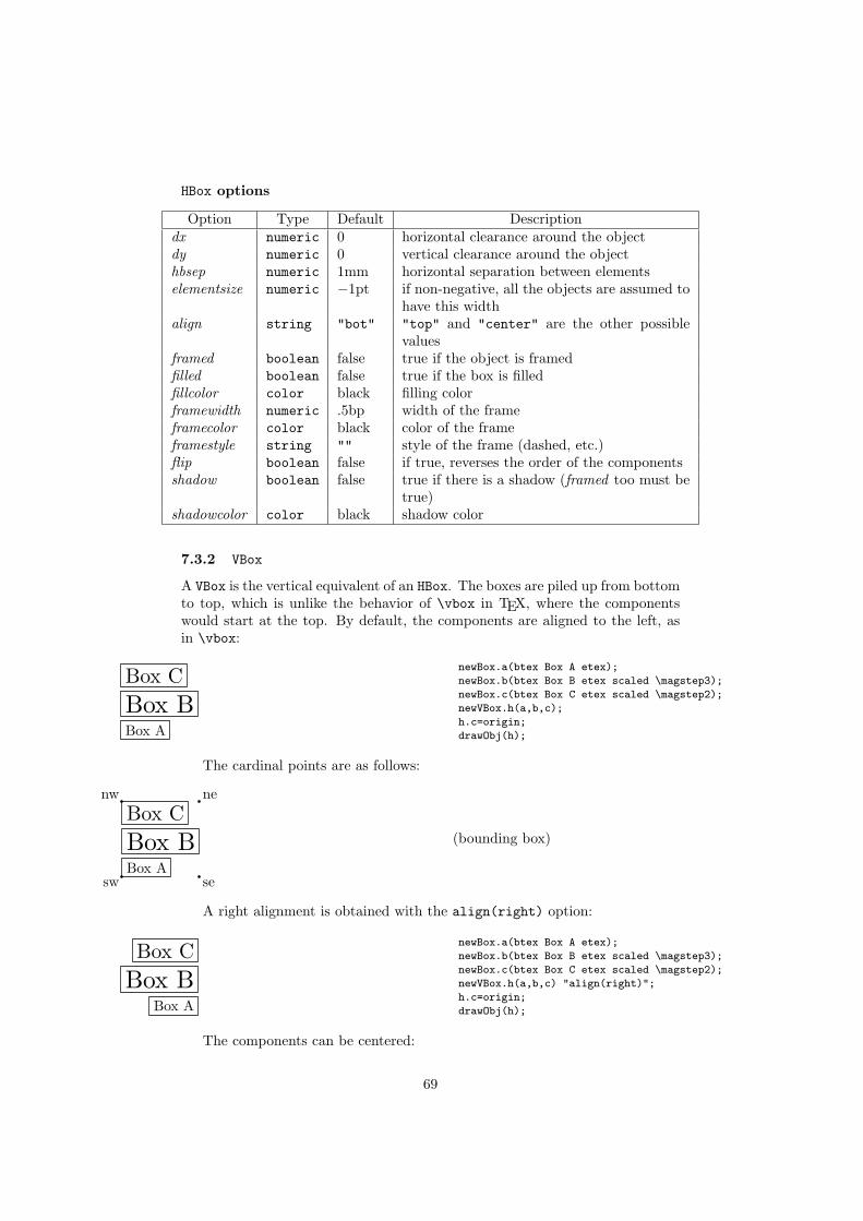
HBox options
Option Type Default Descriptiondx numeric 0 horizontal clearance around the objectdy numeric 0 vertical clearance around the objecthbsep numeric 1mm horizontal separation between elementselementsize numeric −1pt if non-negative, all the objects are assumed to
have this widthalign string "bot" "top" and "center" are the other possible
valuesframed boolean false true if the object is framedfilled boolean false true if the box is filledfillcolor color black filling colorframewidth numeric .5bp width of the frameframecolor color black color of the frameframestyle string "" style of the frame (dashed, etc.)flip boolean false if true, reverses the order of the componentsshadow boolean false true if there is a shadow (framed too must be
true)shadowcolor color black shadow color
7.3.2 VBox
A VBox is the vertical equivalent of an HBox. The boxes are piled up from bottomto top, which is unlike the behavior of \vbox in TEX, where the componentswould start at the top. By default, the components are aligned to the left, asin \vbox:
Box A
Box BBox C newBox.a(btex Box A etex);
newBox.b(btex Box B etex scaled \magstep3);
newBox.c(btex Box C etex scaled \magstep2);
newVBox.h(a,b,c);
h.c=origin;
drawObj(h);
The cardinal points are as follows:
Box A
Box BBox C
nw ne
sw se
(bounding box)
A right alignment is obtained with the align(right) option:
Box A
Box BBox C newBox.a(btex Box A etex);
newBox.b(btex Box B etex scaled \magstep3);
newBox.c(btex Box C etex scaled \magstep2);
newVBox.h(a,b,c) "align(right)";
h.c=origin;
drawObj(h);
The components can be centered:
69

Box A
Box BBox C newBox.a(btex Box A etex);
newBox.b(btex Box B etex scaled \magstep3);
newBox.c(btex Box C etex scaled \magstep2);
newVBox.h(a,b,c) "align(center)";
h.c=origin;
drawObj(h);
As for HBox, the vertical separation between components can be changedwith the vsep option:
Box A
Box B
Box C newBox.a(btex Box A etex);
newBox.b(btex Box B etex scaled \magstep3);
newBox.c(btex Box C etex scaled \magstep2);
newVBox.h(a,b,c)
"align(center)","vsep(3mm)";
h.c=origin;
drawObj(h);
And it is possible to put any kind of object instead of mere boxes:
Box A
Box B
Box CnewPolygon.a(btex Box A etex,5)
"fit(false)","polymargin(5mm)";
newBox.b(btex Box B etex scaled \magstep3);
newVRazor.ba(1cm);
newPolygon.c(btex Box C etex scaled \magstep2,11)
"polymargin(3mm)";
newVBox.h(a,b,ba,c)
"align(center)","vsep(3mm)";
h.c=origin;
drawObj(h);
VBox options
Option Type Default Descriptiondx numeric 0 horizontal clearance around the objectdy numeric 0 vertical clearance around the objectvbsep numeric 1mm vertical separation between elementselementsize numeric −1pt if non-negative, all the objects are assumed to
have this heightalign string "left" "center" and "right" are the other possible
valuesframed boolean false true if the object is framedfilled boolean false true if the box is filledfillcolor color black filling colorframewidth numeric .5bp width of the frameframecolor color black color of the frameframestyle string "" style of the frame (dashed, etc.)flip boolean false if true, reverses the order of the componentsshadow boolean false true if there is a shadow (framed too must be
true)shadowcolor color black shadow color
70

7.4 Recursive objects and fractals
metaobj provides several standard objects whose purpose is to show how re-cursive objects can be defined.
7.4.1 RecursiveBox
This is one of the simplest kind of recursive object. It is a box which containsa box slightly rotated, which itself contains such a box, etc. The depth of thebox is a parameter of the constructor.
newRecursiveBox.a(10);
scaleObj(a,.3);
a.c=origin;
drawObj(a);
The bounding box has no surprises:
nw ne
sw se
(bounding box)
RecursiveBox options The options recognized by the RecursiveBox objectsare shown in table 4.
71
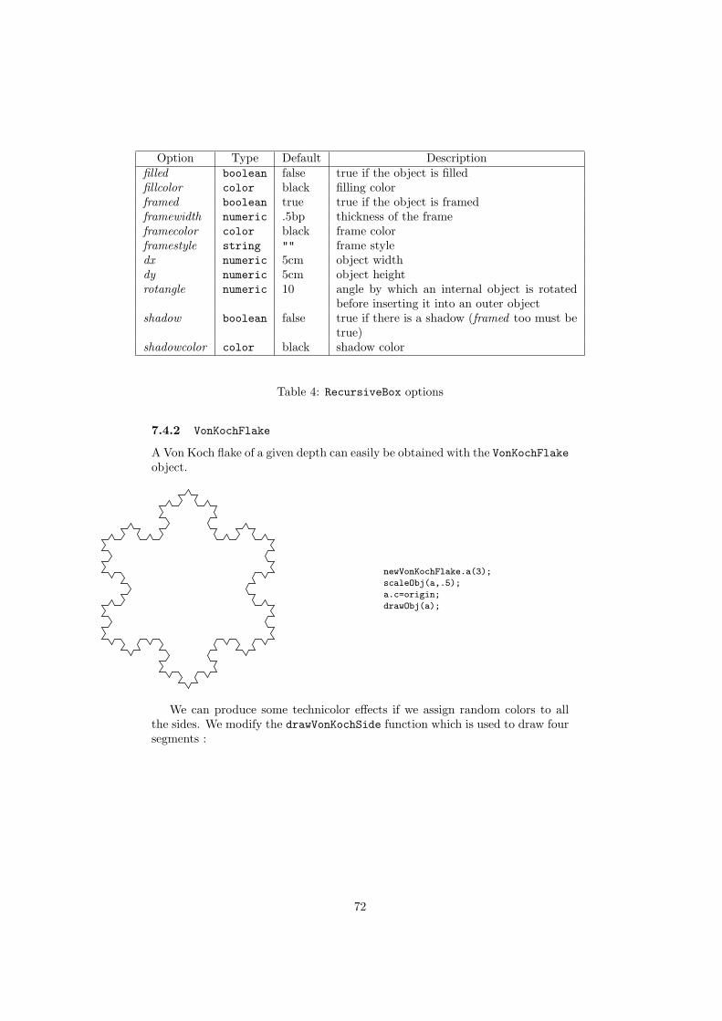
Option Type Default Descriptionfilled boolean false true if the object is filledfillcolor color black filling colorframed boolean true true if the object is framedframewidth numeric .5bp thickness of the frameframecolor color black frame colorframestyle string "" frame styledx numeric 5cm object widthdy numeric 5cm object heightrotangle numeric 10 angle by which an internal object is rotated
before inserting it into an outer objectshadow boolean false true if there is a shadow (framed too must be
true)shadowcolor color black shadow color
Table 4: RecursiveBox options
7.4.2 VonKochFlake
A Von Koch flake of a given depth can easily be obtained with the VonKochFlakeobject.
newVonKochFlake.a(3);
scaleObj(a,.5);
a.c=origin;
drawObj(a);
We can produce some technicolor effects if we assign random colors to allthe sides. We modify the drawVonKochSide function which is used to draw foursegments :
72
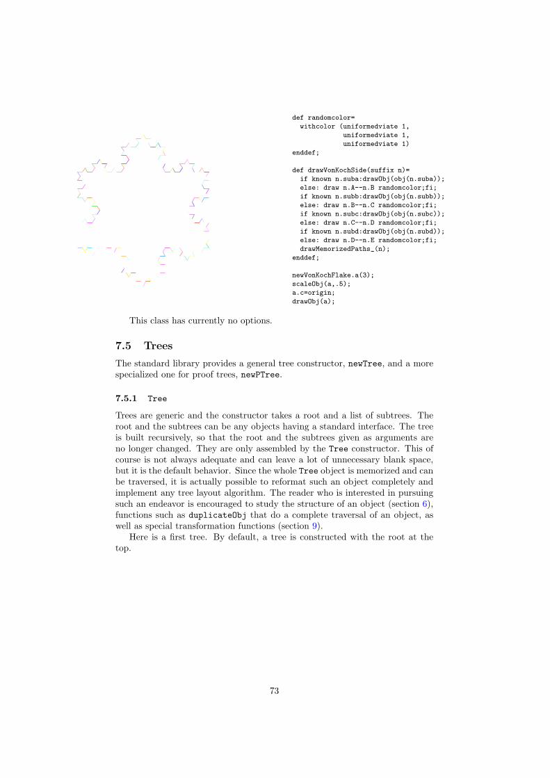
def randomcolor=
withcolor (uniformedviate 1,
uniformedviate 1,
uniformedviate 1)
enddef;
def drawVonKochSide(suffix n)=
if known n.suba:drawObj(obj(n.suba));
else: draw n.A--n.B randomcolor;fi;
if known n.subb:drawObj(obj(n.subb));
else: draw n.B--n.C randomcolor;fi;
if known n.subc:drawObj(obj(n.subc));
else: draw n.C--n.D randomcolor;fi;
if known n.subd:drawObj(obj(n.subd));
else: draw n.D--n.E randomcolor;fi;
drawMemorizedPaths_(n);
enddef;
newVonKochFlake.a(3);
scaleObj(a,.5);
a.c=origin;
drawObj(a);
This class has currently no options.
7.5 Trees
The standard library provides a general tree constructor, newTree, and a morespecialized one for proof trees, newPTree.
7.5.1 Tree
Trees are generic and the constructor takes a root and a list of subtrees. Theroot and the subtrees can be any objects having a standard interface. The treeis built recursively, so that the root and the subtrees given as arguments areno longer changed. They are only assembled by the Tree constructor. This ofcourse is not always adequate and can leave a lot of unnecessary blank space,but it is the default behavior. Since the whole Tree object is memorized and canbe traversed, it is actually possible to reformat such an object completely andimplement any tree layout algorithm. The reader who is interested in pursuingsuch an endeavor is encouraged to study the structure of an object (section 6),functions such as duplicateObj that do a complete traversal of an object, aswell as special transformation functions (section 9).
Here is a first tree. By default, a tree is constructed with the root at thetop.
73
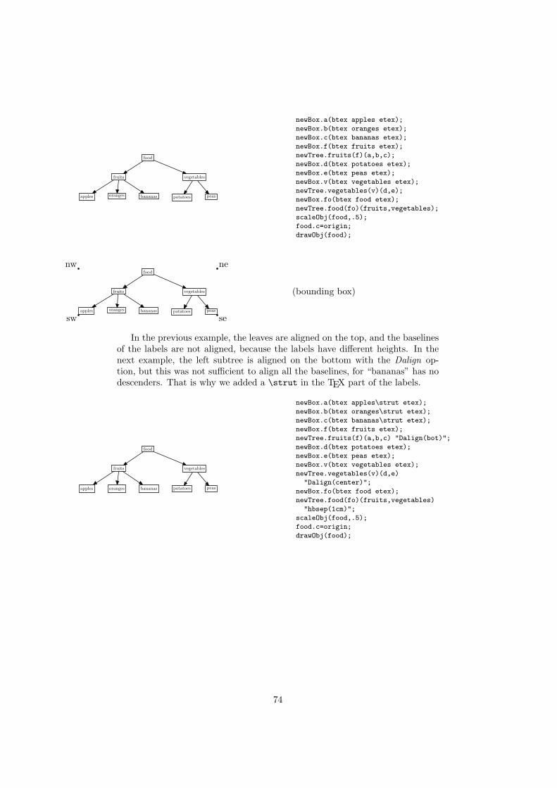
apples oranges bananas
fruits
potatoes peas
vegetables
food
newBox.a(btex apples etex);
newBox.b(btex oranges etex);
newBox.c(btex bananas etex);
newBox.f(btex fruits etex);
newTree.fruits(f)(a,b,c);
newBox.d(btex potatoes etex);
newBox.e(btex peas etex);
newBox.v(btex vegetables etex);
newTree.vegetables(v)(d,e);
newBox.fo(btex food etex);
newTree.food(fo)(fruits,vegetables);
scaleObj(food,.5);
food.c=origin;
drawObj(food);
apples oranges bananas
fruits
potatoes peas
vegetables
foodnw ne
sw se
(bounding box)
In the previous example, the leaves are aligned on the top, and the baselinesof the labels are not aligned, because the labels have different heights. In thenext example, the left subtree is aligned on the bottom with the Dalign op-tion, but this was not sufficient to align all the baselines, for “bananas” has nodescenders. That is why we added a \strut in the TEX part of the labels.
apples oranges bananas
fruits
potatoes peas
vegetables
food
newBox.a(btex apples\strut etex);
newBox.b(btex oranges\strut etex);
newBox.c(btex bananas\strut etex);
newBox.f(btex fruits etex);
newTree.fruits(f)(a,b,c) "Dalign(bot)";
newBox.d(btex potatoes etex);
newBox.e(btex peas etex);
newBox.v(btex vegetables etex);
newTree.vegetables(v)(d,e)
"Dalign(center)";
newBox.fo(btex food etex);
newTree.food(fo)(fruits,vegetables)
"hbsep(1cm)";
scaleObj(food,.5);
food.c=origin;
drawObj(food);
74
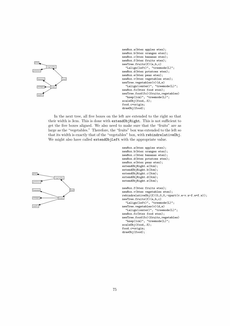
apples
oranges
bananas
fruits
potatoes
peas
vegetables
food
newBox.a(btex apples etex);
newBox.b(btex oranges etex);
newBox.c(btex bananas etex);
newBox.f(btex fruits etex);
newTree.fruits(f)(a,b,c)
"Lalign(left)", "treemode(L)";
newBox.d(btex potatoes etex);
newBox.e(btex peas etex);
newBox.v(btex vegetables etex);
newTree.vegetables(v)(d,e)
"Lalign(center)", "treemode(L)";
newBox.fo(btex food etex);
newTree.food(fo)(fruits,vegetables)
"hsep(1cm)", "treemode(L)";
scaleObj(food,.5);
food.c=origin;
drawObj(food);
In the next tree, all five boxes on the left are extended to the right so thattheir width is 3cm. This is done with extendObjRight. This is not sufficient toget the five boxes aligned. We also need to make sure that the “fruits” are aslarge as the “vegetables.” Therefore, the “fruits” box was extended to the left sothat its width is exactly that of the “vegetables” box, with rebindrelativeObj.We might also have called extendObjLeft with the appropriate value.
apples
oranges
bananas
fruits
potatoes
peas
vegetables
food
newBox.a(btex apples etex);
newBox.b(btex oranges etex);
newBox.c(btex bananas etex);
newBox.d(btex potatoes etex);
newBox.e(btex peas etex);
extendObjRight.a(3cm);
extendObjRight.b(3cm);
extendObjRight.c(3cm);
extendObjRight.d(3cm);
extendObjRight.e(3cm);
newBox.f(btex fruits etex);
newBox.v(btex vegetables etex);
rebindrelativeObj(f)(0,0,0,-xpart(v.e-v.w-f.e+f.w));
newTree.fruits(f)(a,b,c)
"Lalign(left)", "treemode(L)";
newTree.vegetables(v)(d,e)
"Lalign(center)", "treemode(L)";
newBox.fo(btex food etex);
newTree.food(fo)(fruits,vegetables)
"hsep(1cm)", "treemode(L)";
scaleObj(food,.5);
food.c=origin;
drawObj(food);
75
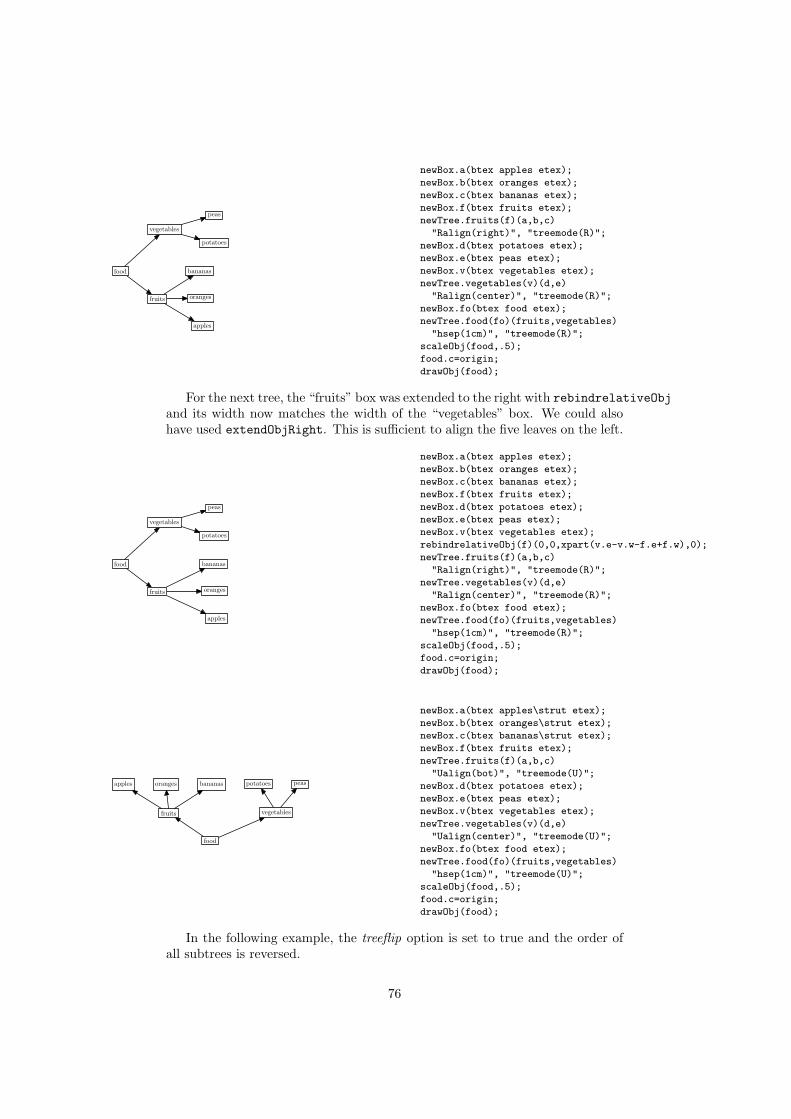
apples
oranges
bananas
fruits
potatoes
peas
vegetables
food
newBox.a(btex apples etex);
newBox.b(btex oranges etex);
newBox.c(btex bananas etex);
newBox.f(btex fruits etex);
newTree.fruits(f)(a,b,c)
"Ralign(right)", "treemode(R)";
newBox.d(btex potatoes etex);
newBox.e(btex peas etex);
newBox.v(btex vegetables etex);
newTree.vegetables(v)(d,e)
"Ralign(center)", "treemode(R)";
newBox.fo(btex food etex);
newTree.food(fo)(fruits,vegetables)
"hsep(1cm)", "treemode(R)";
scaleObj(food,.5);
food.c=origin;
drawObj(food);
For the next tree, the “fruits” box was extended to the right with rebindrelativeObjand its width now matches the width of the “vegetables” box. We could alsohave used extendObjRight. This is sufficient to align the five leaves on the left.
apples
oranges
bananas
fruits
potatoes
peas
vegetables
food
newBox.a(btex apples etex);
newBox.b(btex oranges etex);
newBox.c(btex bananas etex);
newBox.f(btex fruits etex);
newBox.d(btex potatoes etex);
newBox.e(btex peas etex);
newBox.v(btex vegetables etex);
rebindrelativeObj(f)(0,0,xpart(v.e-v.w-f.e+f.w),0);
newTree.fruits(f)(a,b,c)
"Ralign(right)", "treemode(R)";
newTree.vegetables(v)(d,e)
"Ralign(center)", "treemode(R)";
newBox.fo(btex food etex);
newTree.food(fo)(fruits,vegetables)
"hsep(1cm)", "treemode(R)";
scaleObj(food,.5);
food.c=origin;
drawObj(food);
apples oranges bananas
fruits
potatoes peas
vegetables
food
newBox.a(btex apples\strut etex);
newBox.b(btex oranges\strut etex);
newBox.c(btex bananas\strut etex);
newBox.f(btex fruits etex);
newTree.fruits(f)(a,b,c)
"Ualign(bot)", "treemode(U)";
newBox.d(btex potatoes etex);
newBox.e(btex peas etex);
newBox.v(btex vegetables etex);
newTree.vegetables(v)(d,e)
"Ualign(center)", "treemode(U)";
newBox.fo(btex food etex);
newTree.food(fo)(fruits,vegetables)
"hsep(1cm)", "treemode(U)";
scaleObj(food,.5);
food.c=origin;
drawObj(food);
In the following example, the treeflip option is set to true and the order ofall subtrees is reversed.
76
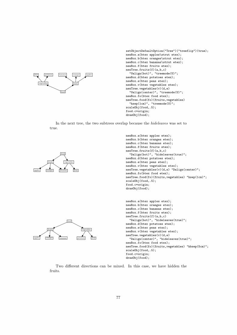
peas potatoes
vegetables
bananas oranges apples
fruits
food
setObjectDefaultOption("Tree")("treeflip")(true);
newBox.a(btex apples\strut etex);
newBox.b(btex oranges\strut etex);
newBox.c(btex bananas\strut etex);
newBox.f(btex fruits etex);
newTree.fruits(f)(a,b,c)
"Ualign(bot)", "treemode(U)";
newBox.d(btex potatoes etex);
newBox.e(btex peas etex);
newBox.v(btex vegetables etex);
newTree.vegetables(v)(d,e)
"Ualign(center)", "treemode(U)";
newBox.fo(btex food etex);
newTree.food(fo)(fruits,vegetables)
"hsep(1cm)", "treemode(U)";
scaleObj(food,.5);
food.c=origin;
drawObj(food);
In the next tree, the two subtrees overlap because the hideleaves was set totrue.
apples oranges bananas
fruits
potatoes peas
vegetables
food
newBox.a(btex apples etex);
newBox.b(btex oranges etex);
newBox.c(btex bananas etex);
newBox.f(btex fruits etex);
newTree.fruits(f)(a,b,c)
"Dalign(bot)", "hideleaves(true)";
newBox.d(btex potatoes etex);
newBox.e(btex peas etex);
newBox.v(btex vegetables etex);
newTree.vegetables(v)(d,e) "Dalign(center)";
newBox.fo(btex food etex);
newTree.food(fo)(fruits,vegetables) "hsep(1cm)";
scaleObj(food,.5);
food.c=origin;
drawObj(food);
apples oranges bananas
fruits
potatoes peas
vegetables
food
newBox.a(btex apples etex);
newBox.b(btex oranges etex);
newBox.c(btex bananas etex);
newBox.f(btex fruits etex);
newTree.fruits(f)(a,b,c)
"Dalign(bot)", "hideleaves(true)";
newBox.d(btex potatoes etex);
newBox.e(btex peas etex);
newBox.v(btex vegetables etex);
newTree.vegetables(v)(d,e)
"Dalign(center)", "hideleaves(true)";
newBox.fo(btex food etex);
newTree.food(fo)(fruits,vegetables) "hbsep(5cm)";
scaleObj(food,.5);
food.c=origin;
drawObj(food);
Two different directions can be mixed. In this case, we have hidden thefruits.
77
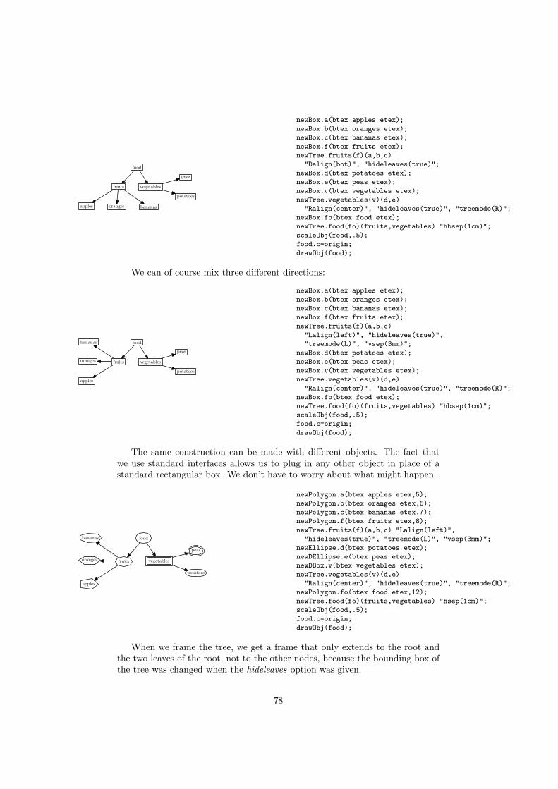
apples oranges bananas
fruits
potatoes
peas
vegetables
food
newBox.a(btex apples etex);
newBox.b(btex oranges etex);
newBox.c(btex bananas etex);
newBox.f(btex fruits etex);
newTree.fruits(f)(a,b,c)
"Dalign(bot)", "hideleaves(true)";
newBox.d(btex potatoes etex);
newBox.e(btex peas etex);
newBox.v(btex vegetables etex);
newTree.vegetables(v)(d,e)
"Ralign(center)", "hideleaves(true)", "treemode(R)";
newBox.fo(btex food etex);
newTree.food(fo)(fruits,vegetables) "hbsep(1cm)";
scaleObj(food,.5);
food.c=origin;
drawObj(food);
We can of course mix three different directions:
apples
oranges
bananas
fruits
potatoes
peas
vegetables
food
newBox.a(btex apples etex);
newBox.b(btex oranges etex);
newBox.c(btex bananas etex);
newBox.f(btex fruits etex);
newTree.fruits(f)(a,b,c)
"Lalign(left)", "hideleaves(true)",
"treemode(L)", "vsep(3mm)";
newBox.d(btex potatoes etex);
newBox.e(btex peas etex);
newBox.v(btex vegetables etex);
newTree.vegetables(v)(d,e)
"Ralign(center)", "hideleaves(true)", "treemode(R)";
newBox.fo(btex food etex);
newTree.food(fo)(fruits,vegetables) "hbsep(1cm)";
scaleObj(food,.5);
food.c=origin;
drawObj(food);
The same construction can be made with different objects. The fact thatwe use standard interfaces allows us to plug in any other object in place of astandard rectangular box. We don’t have to worry about what might happen.
apples
oranges
bananas
fruits
potatoes
peas
vegetables
food
newPolygon.a(btex apples etex,5);
newPolygon.b(btex oranges etex,6);
newPolygon.c(btex bananas etex,7);
newPolygon.f(btex fruits etex,8);
newTree.fruits(f)(a,b,c) "Lalign(left)",
"hideleaves(true)", "treemode(L)", "vsep(3mm)";
newEllipse.d(btex potatoes etex);
newDEllipse.e(btex peas etex);
newDBox.v(btex vegetables etex);
newTree.vegetables(v)(d,e)
"Ralign(center)", "hideleaves(true)", "treemode(R)";
newPolygon.fo(btex food etex,12);
newTree.food(fo)(fruits,vegetables) "hsep(1cm)";
scaleObj(food,.5);
food.c=origin;
drawObj(food);
When we frame the tree, we get a frame that only extends to the root andthe two leaves of the root, not to the other nodes, because the bounding box ofthe tree was changed when the hideleaves option was given.
78
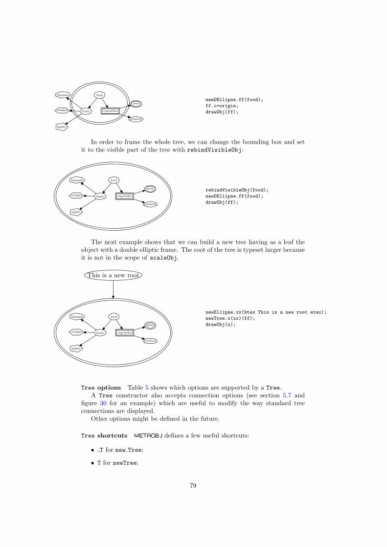
apples
oranges
bananas
fruits
potatoes
peas
vegetables
foodnewDEllipse.ff(food);
ff.c=origin;
drawObj(ff);
In order to frame the whole tree, we can change the bounding box and setit to the visible part of the tree with rebindVisibleObj:
apples
oranges
bananas
fruits
potatoes
peas
vegetables
food
rebindVisibleObj(food);
newDEllipse.ff(food);
drawObj(ff);
The next example shows that we can build a new tree having as a leaf theobject with a double elliptic frame. The root of the tree is typeset larger becauseit is not in the scope of scaleObj.
apples
oranges
bananas
fruits
potatoes
peas
vegetables
food
This is a new root
newEllipse.xx(btex This is a new root etex);
newTree.x(xx)(ff);
drawObj(x);
Tree options Table 5 shows which options are supported by a Tree.A Tree constructor also accepts connection options (see section 5.7 and
figure 30 for an example) which are useful to modify the way standard treeconnections are displayed.
Other options might be defined in the future.
Tree shortcuts metaobj defines a few useful shortcuts:
• T for new Tree;
• T for newTree;
79

Option Type Default Descriptiontreemode string "D" direction in which the tree develops; there are
four different possible values: "D" (default),"U", "L" and "R"
treeflip boolean false if true, reverses the order of the subtreestreenodehsize numeric −1pt if non-negative, all the nodes are assumed to
have this widthtreenodevsize numeric −1pt if non-negative, all the nodes are assumed to
have this heightdx numeric 0 horizontal clearance around the treedy numeric 0 vertical clearance around the treehsep numeric 1cm for a horizontal tree, this is the separation be-
tween the root and the subtreesvsep numeric 1cm for a vertical tree, this is the separation be-
tween the root and the subtreeshbsep numeric 1cm for a vertical tree, this is the horizontal separa-
tion between subtrees; the subtrees are actu-ally put in a HBox and the value of this optionis passed to the HBox constructor
vbsep numeric 1cm for an horizontal tree, this is the vertical sepa-ration between subtrees; the subtrees are actu-ally put in a VBox and the value of this optionis passed to the VBox constructor
hideleaves boolean false if true, the subtrees are not taken into accountin the bounding box
edge string "ncline" name of a connection commandframed boolean false true if the tree is framedfilled boolean false true of the tree is filledfillcolor color black filling colorframewidth numeric .5bp thickness of the frameframecolor color black color of the frameframestyle string "" style of the frameDalign string "top" vertical alignment of subtrees for trees that go
down (the root on the top); the other possiblevalues are "center" and "bot"
Ualign string "bot" vertical alignment of subtrees for trees that goup (the root on the bottom); the other possiblevalues are "center" and "top"
Lalign string "right" horizontal alignment of subtrees for trees thatgo left (the root on the right); the other pos-sible values are "center" and "left"
Ralign string "left" horizontal alignment of subtrees for trees thatgo right (the root on the left); the other pos-sible values are "center" and "right"
shadow boolean false true if there is a shadow (framed too must betrue)
shadowcolor color black shadow color
Table 5: Tree options
80
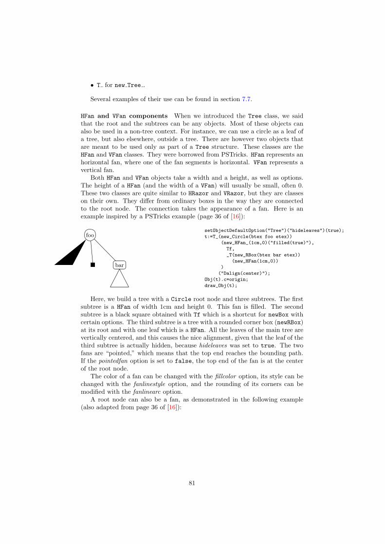
• T for new Tree .
Several examples of their use can be found in section 7.7.
HFan and VFan components When we introduced the Tree class, we saidthat the root and the subtrees can be any objects. Most of these objects canalso be used in a non-tree context. For instance, we can use a circle as a leaf ofa tree, but also elsewhere, outside a tree. There are however two objects thatare meant to be used only as part of a Tree structure. These classes are theHFan and VFan classes. They were borrowed from PSTricks. HFan represents anhorizontal fan, where one of the fan segments is horizontal. VFan represents avertical fan.
Both HFan and VFan objects take a width and a height, as well as options.The height of a HFan (and the width of a VFan) will usually be small, often 0.These two classes are quite similar to HRazor and VRazor, but they are classeson their own. They differ from ordinary boxes in the way they are connectedto the root node. The connection takes the appearance of a fan. Here is anexample inspired by a PSTricks example (page 36 of [16]):
bar
foosetObjectDefaultOption("Tree")("hideleaves")(true);
t:=T_(new_Circle(btex foo etex))
(new_HFan_(1cm,0)("filled(true)"),
Tf,
_T(new_RBox(btex bar etex))
(new_HFan(1cm,0))
)
("Dalign(center)");
Obj(t).c=origin;
draw_Obj(t);
Here, we build a tree with a Circle root node and three subtrees. The firstsubtree is a HFan of width 1cm and height 0. This fan is filled. The secondsubtree is a black square obtained with Tf which is a shortcut for newBox withcertain options. The third subtree is a tree with a rounded corner box (newRBox)at its root and with one leaf which is a HFan. All the leaves of the main tree arevertically centered, and this causes the nice alignment, given that the leaf of thethird subtree is actually hidden, because hideleaves was set to true. The twofans are “pointed,” which means that the top end reaches the bounding path.If the pointedfan option is set to false, the top end of the fan is at the centerof the root node.
The color of a fan can be changed with the fillcolor option, its style can bechanged with the fanlinestyle option, and the rounding of its corners can bemodified with the fanlinearc option.
A root node can also be a fan, as demonstrated in the following example(also adapted from page 36 of [16]):
81

foo
t:=_T(new_Circle(btex foo etex))
(_T(new_HFan_(1cm,0)
("filled(true)",
"fillcolor(red)",
"fanlinearc(1mm)"
)
)
(TC,new_HFan_(1cm,0)
("fanlinestyle(dashed evenly)")));
Obj(t).c=origin;
draw_Obj(t);
Here, the red fan is the root of a subtree. The top of the black disk is alignedwith the bottom of the fan, because descending trees are by default aligned onthe top, and the fan is considered an horizontal line and its top is the sameas its bottom. This wouldn’t have been the case if the second parameter ofnew_HFan_ had been different to 0.
HFan and VFan options The two classes have exactly the same options:
Option Type Defaultfilled boolean falsefillcolor color blackedge string "yes"pointedfan boolean truefanlinestyle string ""fanlinearc numeric 0
Most of these options have been explained. The edge option is a string whichby default is "yes". This means that the fan edges must be drawn. There arecertain cases where we want fans to skip levels and one way of achieving it is toset edge to "none". A more elaborate example is given in figure 40.
Incremental construction of trees Two commands make it possible tobuild a Tree incrementally, and even to replace a subtree by another and havethe tree adjust automatically. These commands are replaceTreeElement.expland deleteTreeElement.expl3. They are experimental commands and are notsupported. They only work in certain cases and have side-effects.
The side-effect of the two experimental commands is that they reset thetree. This means that if the tree had been transformed (rotated, scaled, ...),it will be reset to a non-transformed stage. Moreover, all its components willhave the same fate, and this may reset the tree in a state different from theinitial state. metaobj currently doesn’t store enough information to properlyreset an object in all cases, and all the commands using the reset operation,such as replaceTreeElement.expl and deleteTreeElement.expl can haveunexpected results.
7.5.2 PTree
The PTree object is designed for proof trees. It provides for either top-downtrees or bottom-up trees. Several other objects are associated to the PTreeobject:
3All the experimental commands have a name ending in .expl.
82
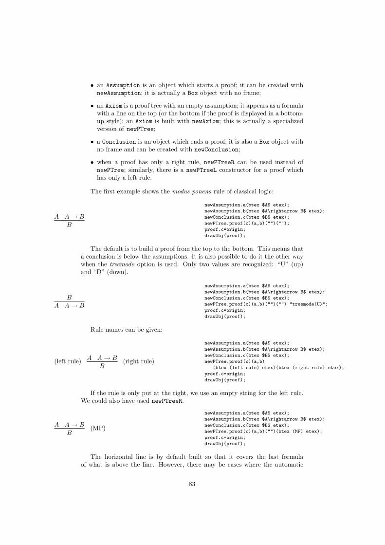
• an Assumption is an object which starts a proof; it can be created withnewAssumption; it is actually a Box object with no frame;
• an Axiom is a proof tree with an empty assumption; it appears as a formulawith a line on the top (or the bottom if the proof is displayed in a bottom-up style); an Axiom is built with newAxiom; this is actually a specializedversion of newPTree;
• a Conclusion is an object which ends a proof; it is also a Box object withno frame and can be created with newConclusion;
• when a proof has only a right rule, newPTreeR can be used instead ofnewPTree; similarly, there is a newPTreeL constructor for a proof whichhas only a left rule.
The first example shows the modus ponens rule of classical logic:
B
A A → B
newAssumption.a(btex $A$ etex);
newAssumption.b(btex $A\rightarrow B$ etex);
newConclusion.c(btex $B$ etex);
newPTree.proof(c)(a,b)("")("");
proof.c=origin;
drawObj(proof);
The default is to build a proof from the top to the bottom. This means thata conclusion is below the assumptions. It is also possible to do it the other waywhen the treemode option is used. Only two values are recognized: “U” (up)and “D” (down).
B
A A → B
newAssumption.a(btex $A$ etex);
newAssumption.b(btex $A\rightarrow B$ etex);
newConclusion.c(btex $B$ etex);
newPTree.proof(c)(a,b)("")("") "treemode(U)";
proof.c=origin;
drawObj(proof);
Rule names can be given:
B
A A → B(left rule) (right rule)
newAssumption.a(btex $A$ etex);
newAssumption.b(btex $A\rightarrow B$ etex);
newConclusion.c(btex $B$ etex);
newPTree.proof(c)(a,b)
(btex (left rule) etex)(btex (right rule) etex);
proof.c=origin;
drawObj(proof);
If the rule is only put at the right, we use an empty string for the left rule.We could also have used newPTreeR.
B
A A → B (MP)
newAssumption.a(btex $A$ etex);
newAssumption.b(btex $A\rightarrow B$ etex);
newConclusion.c(btex $B$ etex);
newPTree.proof(c)(a,b)("")(btex (MP) etex);
proof.c=origin;
drawObj(proof);
The horizontal line is by default built so that it covers the last formulaof what is above the line. However, there may be cases where the automatic
83

computation is not satisfactory and it is then possible to change the length ofthe line, by extending its right or left ends. In order to lengthen the right endby 1cm, we can pass 1cm to the lenddx option of newPTree (or its variants):
B
A A → B (MP)
newAssumption.a(btex $A$ etex);
newAssumption.b(btex $A\rightarrow B$ etex);
newConclusion.c(btex $B$ etex);
newPTreeR.proof(c)(a,b)(btex (MP) etex)
"lenddx(1cm)";
proof.c=origin;
drawObj(proof);
Transformations can be applied to a proof, as for any other object:
BA A → B (MP)
scaleObj(proof,2);
slantObj(proof,1);
proof.c=origin;
drawObj(proof);
The next example shows that it is possible to have two overlapping proofs.The first two lines are one proof, built top-down, and this proof is also theconclusion of a second proof, built bottom-up and whose assumptions are thetwo formulas on the last line.
B
A A → B (MP)
D E
newAssumption.a(btex $A$ etex);
newAssumption.b(btex $A\rightarrow B$ etex);
newConclusion.c(btex $B$ etex);
newAssumption.d(btex $D$ etex);
newAssumption.e(btex $E$ etex);
newPTreeR.proof1(c)(a,b)(btex (MP) etex);
newPTreeR.proof2(proof1)(d,e)("")
"treemode(U)";
proof2.c=origin;
drawObj(proof2);
This is another such example where the intermediate formula is wider thanthe others.
BBBBBBBBBBBBBB
A A → B (MP)
D E
newAssumption.a(btex $A$ etex);
newAssumption.b(btex $A\rightarrow B$ etex);
newConclusion.c(btex $BBBBBBBBBBBBBB$ etex);
newAssumption.d(btex $D$ etex);
newAssumption.e(btex $E$ etex);
newPTreeR.proof1(c)(a,b)(btex (MP) etex);
newPTreeR.proof2(proof1)(d,e)("")
"treemode(U)";
proof2.c=origin;
drawObj(proof2);
A more elaborate proof tree is given in figure 7. The source file defines aTEX command to obtain a column of n dots. The top-down proof is the defaultand the bottom-up proof is obtained by specifying:
setObjectDefaultOption("PTree")("treemode")("U");
Though the result is quite acceptable, one must admit that writing such aproof in metaobj directly is not that practical. In this case, a TEX interfacefor metaobj would prove very useful and would allow a comparison with otherpackages for proof trees.
PTree options Table 6 shows the options supported by the PTree class.
84
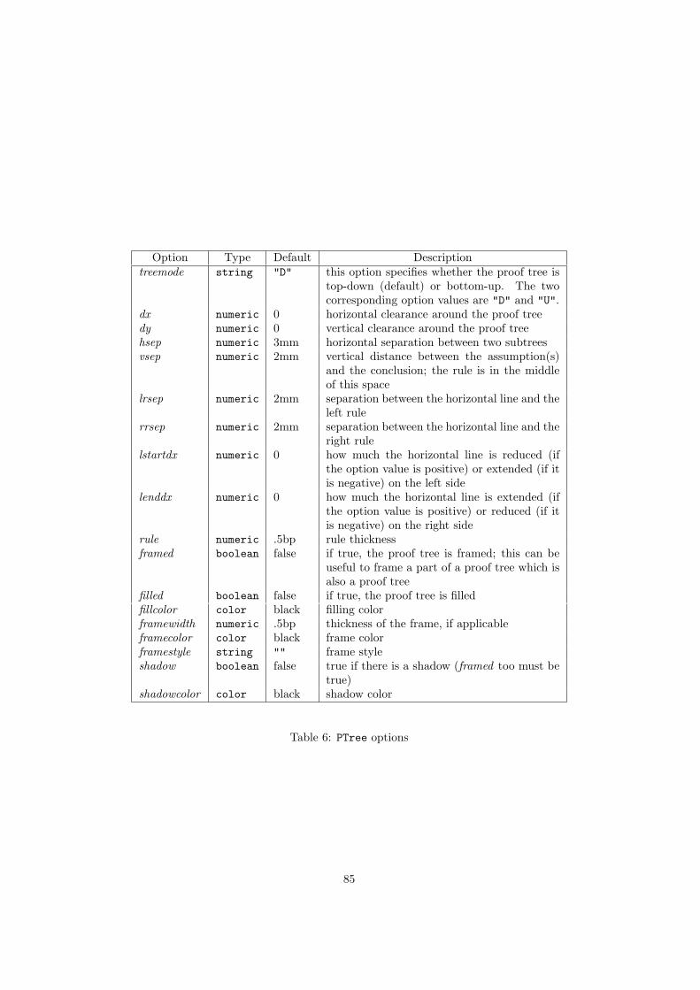
Option Type Default Descriptiontreemode string "D" this option specifies whether the proof tree is
top-down (default) or bottom-up. The twocorresponding option values are "D" and "U".
dx numeric 0 horizontal clearance around the proof treedy numeric 0 vertical clearance around the proof treehsep numeric 3mm horizontal separation between two subtreesvsep numeric 2mm vertical distance between the assumption(s)
and the conclusion; the rule is in the middleof this space
lrsep numeric 2mm separation between the horizontal line and theleft rule
rrsep numeric 2mm separation between the horizontal line and theright rule
lstartdx numeric 0 how much the horizontal line is reduced (ifthe option value is positive) or extended (if itis negative) on the left side
lenddx numeric 0 how much the horizontal line is extended (ifthe option value is positive) or reduced (if itis negative) on the right side
rule numeric .5bp rule thicknessframed boolean false if true, the proof tree is framed; this can be
useful to frame a part of a proof tree which isalso a proof tree
filled boolean false if true, the proof tree is filledfillcolor color black filling colorframewidth numeric .5bp thickness of the frame, if applicableframecolor color black frame colorframestyle string "" frame styleshadow boolean false true if there is a shadow (framed too must be
true)shadowcolor color black shadow color
Table 6: PTree options
85
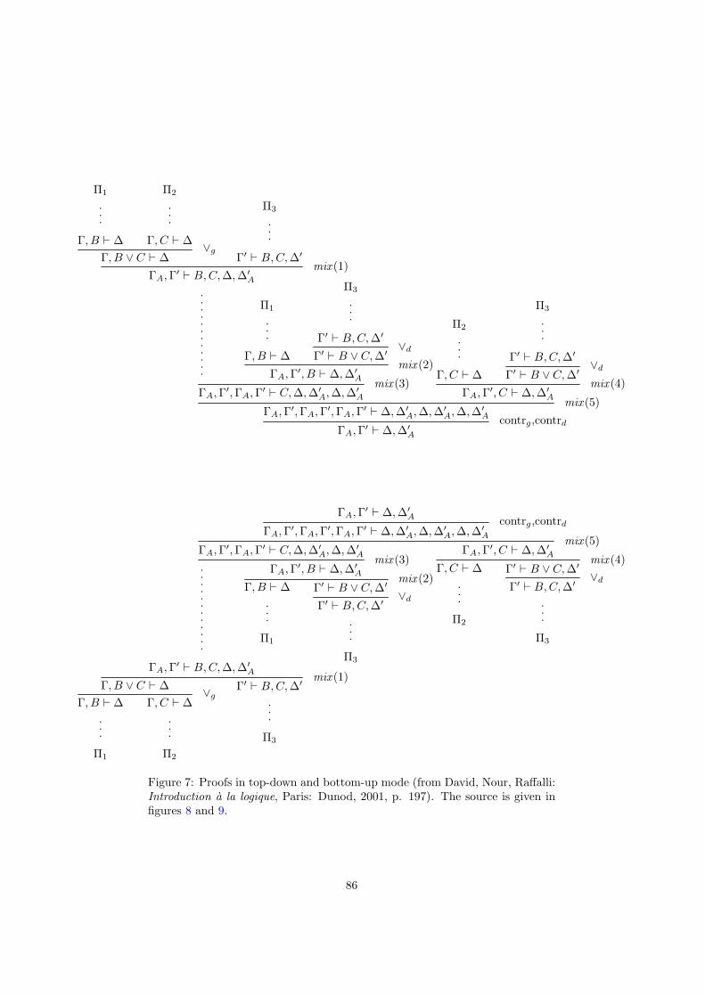
ΓA, Γ′ ` ∆, ∆′A
ΓA, Γ′, ΓA, Γ′, ΓA, Γ′ ` ∆, ∆′A, ∆, ∆′
A, ∆, ∆′A
ΓA, Γ′, ΓA, Γ′ ` C, ∆, ∆′A, ∆, ∆′
A
.
.
.
.
.
.
.
.
.
.
.
.
ΓA, Γ′ ` B,C, ∆, ∆′A
Γ, B ∨ C ` ∆Γ, B ` ∆
.
.
.
Π1
Γ, C ` ∆
.
.
.
Π2
∨gΓ′ ` B,C, ∆′
.
.
.
Π3
mix (1)
ΓA, Γ′, B ` ∆, ∆′A
Γ, B ` ∆
.
.
.
Π1
Γ′ ` B ∨ C, ∆′Γ′ ` B,C, ∆′
.
.
.
Π3
∨d
mix (2)
mix (3)ΓA, Γ′, C ` ∆, ∆′
A
Γ, C ` ∆
.
.
.
Π2
Γ′ ` B ∨ C, ∆′Γ′ ` B,C, ∆′
.
.
.
Π3
∨d
mix (4)
mix (5)contrg,contrd
ΓA, Γ′ ` ∆, ∆′A
ΓA, Γ′, ΓA, Γ′, ΓA, Γ′ ` ∆, ∆′A, ∆, ∆′
A, ∆, ∆′A
ΓA, Γ′, ΓA, Γ′ ` C, ∆, ∆′A, ∆, ∆′
A
.
.
.
.
.
.
.
.
.
.
.
.
ΓA, Γ′ ` B,C, ∆, ∆′A
Γ, B ∨ C ` ∆Γ, B ` ∆
.
.
.
Π1
Γ, C ` ∆...
Π2
∨gΓ′ ` B,C, ∆′
.
.
.
Π3
mix (1)
ΓA, Γ′, B ` ∆, ∆′A
Γ, B ` ∆...
Π1
Γ′ ` B ∨ C, ∆′
Γ′ ` B,C, ∆′
.
.
.
Π3
∨d
mix (2)
mix (3)ΓA, Γ′, C ` ∆, ∆′
A
Γ, C ` ∆...
Π2
Γ′ ` B ∨ C, ∆′
Γ′ ` B,C, ∆′
.
.
.
Π3
∨d
mix (4)
mix (5)
contrg,contrd
Figure 7: Proofs in top-down and bottom-up mode (from David, Nour, Raffalli:Introduction a la logique, Paris: Dunod, 2001, p. 197). The source is given infigures 8 and 9.
86

input metaobj
verbatimtex
\newcount\pntcnt
\pntcnt=0
\def\npoints#1{\pntcnt=#1\vbox{\offinterlineskip\kern5pt\npointsa}}
\def\npointsa{\ifnum\pntcnt>0\hbox{$.$}\kern5pt\advance\pntcnt-1
\expandafter\npointsa\fi}
etex
% setObjectDefaultOption("PTree")("treemode")("U"); % for bottom-up
newAssumption.pi1(btex $\Pi_1$ etex);
newConclusion.pi1c1(btex \npoints3 etex);
newPTreeR.pi1proof(pi1c1)(pi1)("") "rule(0)";
newConclusion.pi1c2(btex $\Gamma,B \vdash \Delta$ etex);
newPTreeR.a1(pi1c2)(pi1proof)("") "rule(0)";
newAssumption.pi2(btex $\Pi_2$ etex);
newConclusion.pi2c1(btex \npoints3 etex);
newPTreeR.pi2proof(pi2c1)(pi2)("") "rule(0)";
newConclusion.pi2c2(btex $\Gamma,C \vdash \Delta$ etex);
newPTreeR.a2(pi2c2)(pi2proof)("") "rule(0)";
newConclusion.c1(btex $\Gamma,B\lor C \vdash \Delta$ etex);
newPTreeR.proof1(c1)(a1,a2)(btex $\lor_g$ etex);
newAssumption.pi3(btex $\Pi_3$ etex);
newConclusion.pi3c1(btex \npoints3 etex);
newPTreeR.pi3proof(pi3c1)(pi3)("") "rule(0)";
newConclusion.pi3c2(btex $\Gamma’ \vdash B,C, \Delta’$ etex);
newPTreeR.a3(pi3c2)(pi3proof)("") "rule(0)";
newConclusion.c2
(btex \Gamma_A,\Gamma’\vdash B,C,\Delta,\Delta’_A etex);
newPTreeR.proof2(c2)(proof1,a3)(btex {\it mix\/}$(1)$ etex);
newConclusion.c2points
(btex \npoints{12} etex);
newPTreeR.proof2a(c2points)(proof2)("") "rule(0)";
duplicateObj(a4,a1);
duplicateObj(a5,a3);
newConclusion.c3(btex $\Gamma’ \vdash B\lor C, \Delta’$ etex);
newPTreeR.proof3(c3)(a5)(btex $\lor_d$ etex);
newConclusion.c4(btex $\Gamma_A,\Gamma’,B \vdash \Delta, \Delta’_A$ etex);
newPTreeR.proof4(c4)(a4,proof3)(btex {\it mix\/}$(2)$ etex);
newConclusion.c5(btex $\Gamma_A,\Gamma’,\Gamma_A,\Gamma’
\vdash C,\Delta, \Delta’_A,\Delta, \Delta’_A$ etex);
newHRazor.hr1(-4cm);
newPTreeR.proof5(c5)(proof2a,hr1,proof4)(btex {\it mix\/}$(3)$ etex);
Figure 8: Proof tree code for figure 7 (beginning)
87

duplicateObj(a6,a2);
duplicateObj(proof3a,proof3);
newConclusion.c7(btex $\Gamma_A,\Gamma’,C
\vdash \Delta, \Delta’_A$ etex);
newPTreeR.proof3b(c7)(a6,proof3a)(btex {\it mix\/}$(4)$ etex);
newConclusion.c8(btex $\Gamma_A,\Gamma’,\Gamma_A,\Gamma’,\Gamma_A,\Gamma’
\vdash \Delta, \Delta’_A,\Delta, \Delta’_A,\Delta, \Delta’_A$ etex);
newPTreeR.proof3d(c8)(proof5,proof3b)(btex {\it mix\/}$(5)$ etex)
"hsep(5mm)";
newConclusion.c9(btex $\Gamma_A,\Gamma’\vdash \Delta, \Delta’_A$ etex);
newPTreeR.proof3E(c9)(proof3d)(btex contr$_g$,contr$_d$ etex);
%yscaleObj(proof3E,2);
%reflectObj(proof3E,(0,0),(0,1));
%slantObj(proof3E,0.2);
proof3E.c=origin;
drawObj(proof3E);
Figure 9: Proof tree code for figure 7 (end)
88
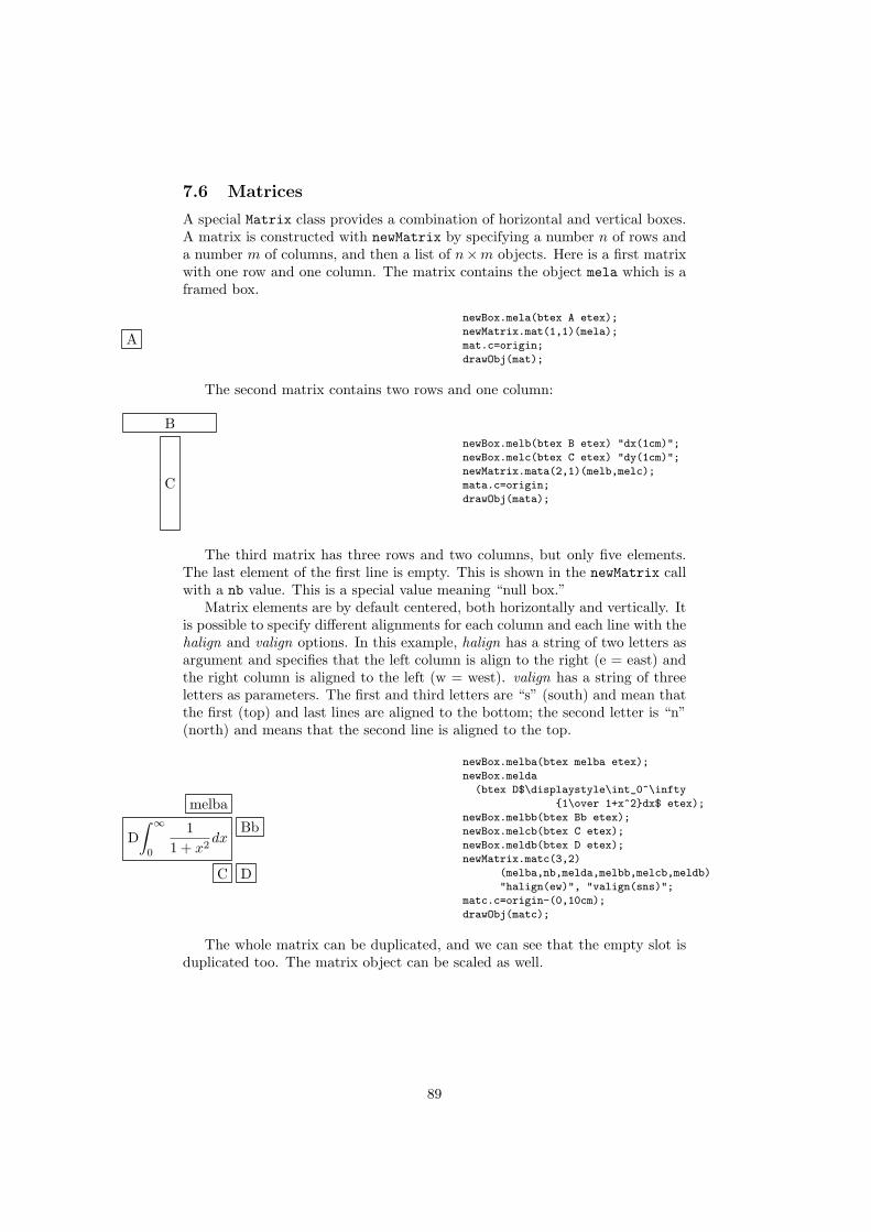
7.6 Matrices
A special Matrix class provides a combination of horizontal and vertical boxes.A matrix is constructed with newMatrix by specifying a number n of rows anda number m of columns, and then a list of n×m objects. Here is a first matrixwith one row and one column. The matrix contains the object mela which is aframed box.
A
newBox.mela(btex A etex);
newMatrix.mat(1,1)(mela);
mat.c=origin;
drawObj(mat);
The second matrix contains two rows and one column:
B
C
newBox.melb(btex B etex) "dx(1cm)";
newBox.melc(btex C etex) "dy(1cm)";
newMatrix.mata(2,1)(melb,melc);
mata.c=origin;
drawObj(mata);
The third matrix has three rows and two columns, but only five elements.The last element of the first line is empty. This is shown in the newMatrix callwith a nb value. This is a special value meaning “null box.”
Matrix elements are by default centered, both horizontally and vertically. Itis possible to specify different alignments for each column and each line with thehalign and valign options. In this example, halign has a string of two letters asargument and specifies that the left column is align to the right (e = east) andthe right column is aligned to the left (w = west). valign has a string of threeletters as parameters. The first and third letters are “s” (south) and mean thatthe first (top) and last lines are aligned to the bottom; the second letter is “n”(north) and means that the second line is aligned to the top.
melba
D∫ ∞
0
11 + x2
dxBb
C D
newBox.melba(btex melba etex);
newBox.melda
(btex D$\displaystyle\int_0^\infty
{1\over 1+x^2}dx$ etex);
newBox.melbb(btex Bb etex);
newBox.melcb(btex C etex);
newBox.meldb(btex D etex);
newMatrix.matc(3,2)
(melba,nb,melda,melbb,melcb,meldb)
"halign(ew)", "valign(sns)";
matc.c=origin-(0,10cm);
drawObj(matc);
The whole matrix can be duplicated, and we can see that the empty slot isduplicated too. The matrix object can be scaled as well.
89

melba
D∫ ∞
0
11 + x2
dxBb
C D
duplicateObj(matd,matc);
scaleObj(matd,2);
matd.c=origin-(0,15cm);
drawObj(matd);
Multispan columns are not implemented. However, it is possible to obtainmultispan-like results by changing the bounding box of a component with theBB wrapper.
7.6.1 Experimental constructions
Experimental commands on matrices are provided: deleteMatrixElement.expland replaceMatrixElement.expl. These commands are not supported. WithreplaceMatrixElement.expl, it is possible to replace a matrix element by an-other, and have the matrix adapt its size to the contents. It is also possible tobuild a Matrix incrementally, starting with a 1× 1 matrix and adding elementsin the same row or in a new row. These two commands have the same problemthan the analog commands for the Tree class.
The next two figures show various replacements.
00000000000000000
D∫ ∞
0
11 + x2
dxBb
C Dnew line
newBox.rep(btex Very Long Replacement etex);
replaceMatrixElement.expl.matd(1,1)(rep);
newBox.repc(btex court etex);
replaceMatrixElement.expl.matd(1,1)(repc);
newBox.repd(btex D etex yscaled 3 rotated 30);
replaceMatrixElement.expl.matd(3,2)(repd);
newBox.repe
(btex 00000000000000000 etex yscaled 3 rotated 30);
replaceMatrixElement.expl.matd(1,1)(repe);
newBox.repf(btex new line etex);
replaceMatrixElement.expl.matd(4,2)(repf);
matd.c=origin;
drawObj(matd);
90
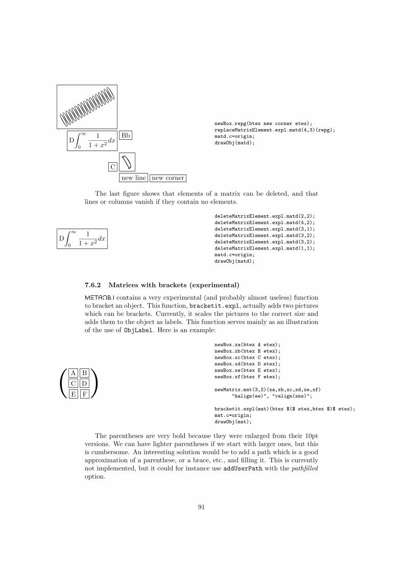
00000000000000000
D∫ ∞
0
11 + x2
dxBb
C Dnew line new corner
newBox.repg(btex new corner etex);
replaceMatrixElement.expl.matd(4,3)(repg);
matd.c=origin;
drawObj(matd);
The last figure shows that elements of a matrix can be deleted, and thatlines or columns vanish if they contain no elements.
D∫ ∞
0
11 + x2
dx
deleteMatrixElement.expl.matd(2,2);
deleteMatrixElement.expl.matd(4,2);
deleteMatrixElement.expl.matd(3,1);
deleteMatrixElement.expl.matd(3,2);
deleteMatrixElement.expl.matd(3,2);
deleteMatrixElement.expl.matd(1,1);
matd.c=origin;
drawObj(matd);
7.6.2 Matrices with brackets (experimental)
metaobj contains a very experimental (and probably almost useless) functionto bracket an object. This function, bracketit.expl, actually adds two pictureswhich can be brackets. Currently, it scales the pictures to the correct size andadds them to the object as labels. This function serves mainly as an illustrationof the use of ObjLabel. Here is an example:
A B
C D
E F( )
newBox.xa(btex A etex);
newBox.xb(btex B etex);
newBox.xc(btex C etex);
newBox.xd(btex D etex);
newBox.xe(btex E etex);
newBox.xf(btex F etex);
newMatrix.mat(3,2)(xa,xb,xc,xd,xe,xf)
"halign(ee)", "valign(sns)";
bracketit.expl(mat)(btex $($ etex,btex $)$ etex);
mat.c=origin;
drawObj(mat);
The parentheses are very bold because they were enlarged from their 10ptversions. We can have lighter parentheses if we start with larger ones, but thisis cumbersome. An interesting solution would be to add a path which is a goodapproximation of a parenthese, or a brace, etc., and filling it. This is currentlynot implemented, but it could for instance use addUserPath with the pathfilledoption.
91
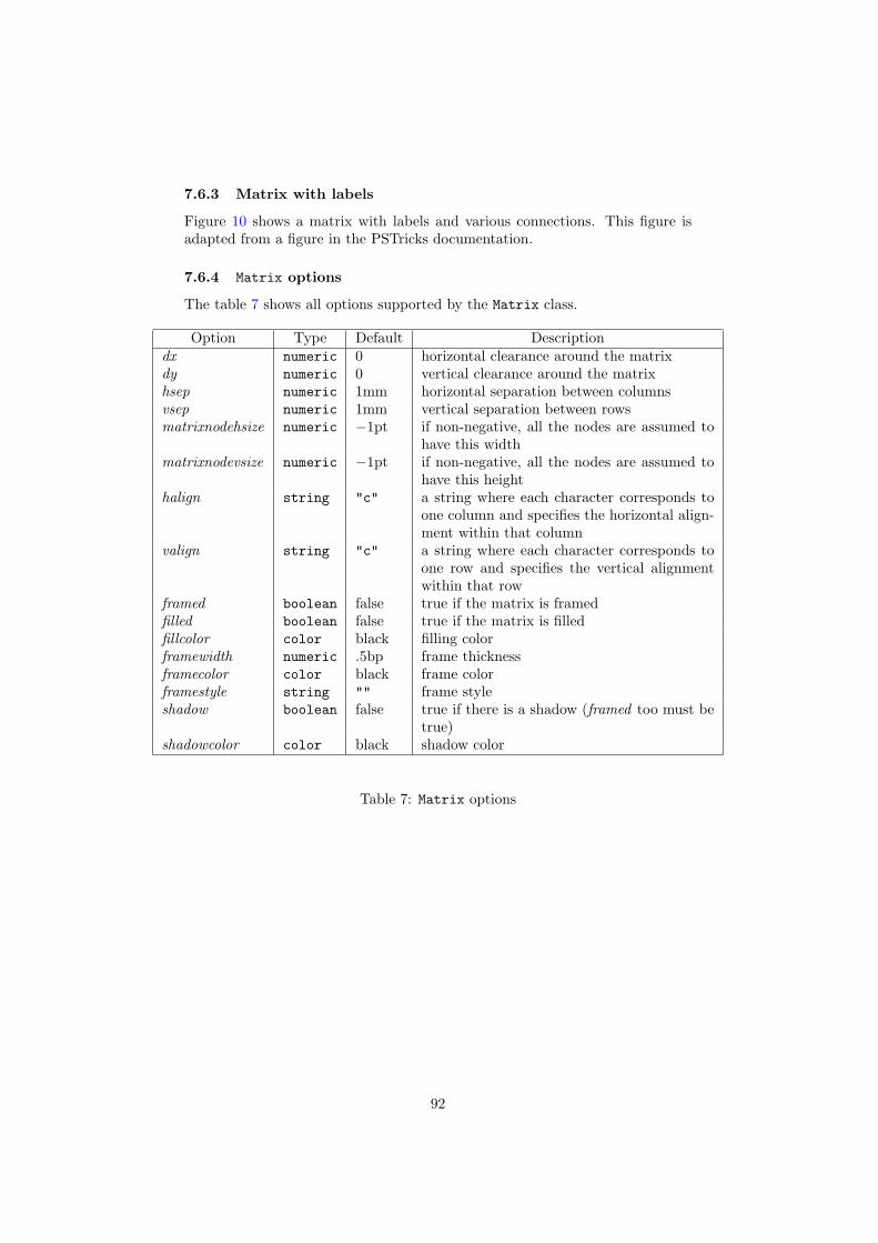
7.6.3 Matrix with labels
Figure 10 shows a matrix with labels and various connections. This figure isadapted from a figure in the PSTricks documentation.
7.6.4 Matrix options
The table 7 shows all options supported by the Matrix class.
Option Type Default Descriptiondx numeric 0 horizontal clearance around the matrixdy numeric 0 vertical clearance around the matrixhsep numeric 1mm horizontal separation between columnsvsep numeric 1mm vertical separation between rowsmatrixnodehsize numeric −1pt if non-negative, all the nodes are assumed to
have this widthmatrixnodevsize numeric −1pt if non-negative, all the nodes are assumed to
have this heighthalign string "c" a string where each character corresponds to
one column and specifies the horizontal align-ment within that column
valign string "c" a string where each character corresponds toone row and specifies the vertical alignmentwithin that row
framed boolean false true if the matrix is framedfilled boolean false true if the matrix is filledfillcolor color black filling colorframewidth numeric .5bp frame thicknessframecolor color black frame colorframestyle string "" frame styleshadow boolean false true if there is a shadow (framed too must be
true)shadowcolor color black shadow color
Table 7: Matrix options
92
7.7 PSTricks/metaobj gallery
metaobj started as a package implementing objects. A basic tenet was thatthe structure of an object had to be available. Then trees were implemented.Then, I had to implement paths, especially for trees, because many examplesof trees I saw had additional paths. It seemed then interesting to have ways toadd PSTricks-like paths. I started to implement functions like ncline, ncbar,etc., corresponding to PSTricks’ \ncline, \ncbar, etc. After some time, theaim was to be able to get good approximations of the PSTricks constructionsinvolving node connections, trees and matrices. metaobj does not provide afull compatibility, neither in the syntax, nor in the output, but it tries to getas close as possible. One should keep in mind that metapost is not TEX,and metapost does not have the same flexibility in its syntax as TEX. It isnot possible to change “catcodes” in metapost or to grab characters one byone. Therefore, the metaobj code corresponding to the PSTricks drawings islonger than the PSTricks’ one. However, it should still be high-level code andunderstandable. It is high-level code written in a syntax less flexible than TEX.What should now be done is to write a TEX front-end to metaobj, which wouldhide the verbosity of metaobj, and still retain high-level code.
On the following pages, we present figures, similar to those found in thePSTricks documentation. PSTricks and metaobj’s parameters do not alwayshave an exact correspondence and even if so, the default values are not alwaysthe same. We tried to produce figures that were close to those produced byPSTricks, but it would be possible to get even better results by better valuesof the parameters. Producing exactly the same result is however not the aimof this section. Our purpose is to show that most features concerning objectsand connections found in PSTricks can be reproduced in metaobj. Whenthe metaobj project started, its purpose was not to mimic PSTricks, andPSTricks-like functionalities were only added at a later stage. metaobj hassome default way of constructing objects and PSTricks has another. Gettingthe exact PSTricks output is possible, but it may need a lot of fiddling. And thiswould certainly be the same if one wanted to mimic metaobj from PSTricks.
93

U
X ×Z Y X
Y Z
yx
pq
g
f
setObjectDefaultOption("Matrix")("hsep")(1cm);
setObjectDefaultOption("Matrix")("vsep")(1cm);
newBox.a(btex $U$ etex) "framed(false)";
newBox.b(btex $X\times_Z Y$ etex) "framed(false)";
newBox.c(btex $X$ etex) "framed(false)";
newBox.d(btex $Y$ etex) "framed(false)";
newBox.e(btex $Z$ etex) "framed(false)";
newMatrix.mat(3,3)(a,nb,nb,nb,b,c,nb,d,e);
mat.c=origin;
mcline.mat(1,1,2,2) "name(a)";
ObjLabel.mat(btex $y$ etex) "labpathname(a)","labdir(llft)";
mcline.mat(1,1,2,3) "doubleline(true)",
"arrows(draw)","linestyle(dashed evenly)", "name(b)";
ObjLabel.mat(btex $x$ etex) "labpathname(b)","labdir(urt)";
mcline.mat(2,2,2,3), "name(c)";
ObjLabel.mat(btex $p$ etex) "labpathname(c)","labdir(bot)";
mcline.mat(2,2,3,2), "name(d)";
ObjLabel.mat(btex $q$ etex) "labpathname(d)","labdir(lft)";
mcline.mat(3,2,3,3), "name(e)";
ObjLabel.mat(btex $g$ etex) "labpathname(e)","labdir(bot)";
mcline.mat(2,3,3,3), "name(f)";
ObjLabel.mat(btex $f$ etex) "labpathname(f)","labdir(rt)";
drawObj(mat);
Figure 10: Matrix example with labels (after page 26 of [16])
94
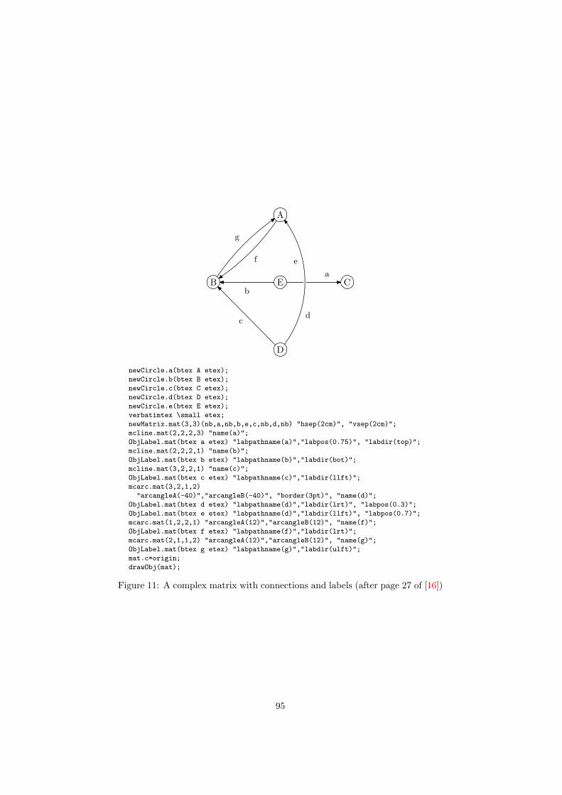
A
B E C
D
a
b
cd
ef
g
newCircle.a(btex A etex);
newCircle.b(btex B etex);
newCircle.c(btex C etex);
newCircle.d(btex D etex);
newCircle.e(btex E etex);
verbatimtex \small etex;
newMatrix.mat(3,3)(nb,a,nb,b,e,c,nb,d,nb) "hsep(2cm)", "vsep(2cm)";
mcline.mat(2,2,2,3) "name(a)";
ObjLabel.mat(btex a etex) "labpathname(a)","labpos(0.75)", "labdir(top)";
mcline.mat(2,2,2,1) "name(b)";
ObjLabel.mat(btex b etex) "labpathname(b)","labdir(bot)";
mcline.mat(3,2,2,1) "name(c)";
ObjLabel.mat(btex c etex) "labpathname(c)","labdir(llft)";
mcarc.mat(3,2,1,2)
"arcangleA(-40)","arcangleB(-40)", "border(3pt)", "name(d)";
ObjLabel.mat(btex d etex) "labpathname(d)","labdir(lrt)", "labpos(0.3)";
ObjLabel.mat(btex e etex) "labpathname(d)","labdir(llft)", "labpos(0.7)";
mcarc.mat(1,2,2,1) "arcangleA(12)","arcangleB(12)", "name(f)";
ObjLabel.mat(btex f etex) "labpathname(f)","labdir(lrt)";
mcarc.mat(2,1,1,2) "arcangleA(12)","arcangleB(12)", "name(g)";
ObjLabel.mat(btex g etex) "labpathname(g)","labdir(ulft)";
mat.c=origin;
drawObj(mat);
Figure 11: A complex matrix with connections and labels (after page 27 of [16])
95
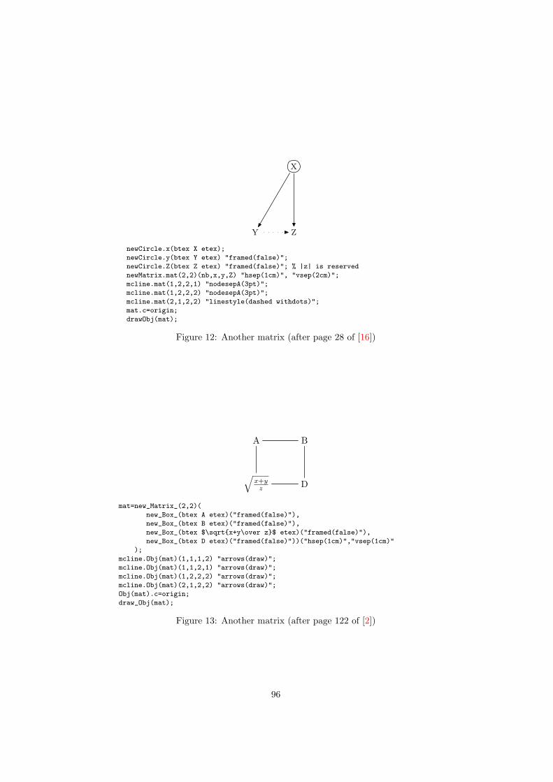
X
Y Z
newCircle.x(btex X etex);
newCircle.y(btex Y etex) "framed(false)";
newCircle.Z(btex Z etex) "framed(false)"; % |z| is reserved
newMatrix.mat(2,2)(nb,x,y,Z) "hsep(1cm)", "vsep(2cm)";
mcline.mat(1,2,2,1) "nodesepA(3pt)";
mcline.mat(1,2,2,2) "nodesepA(3pt)";
mcline.mat(2,1,2,2) "linestyle(dashed withdots)";
mat.c=origin;
drawObj(mat);
Figure 12: Another matrix (after page 28 of [16])
A B
√x+y
z D
mat=new_Matrix_(2,2)(
new_Box_(btex A etex)("framed(false)"),
new_Box_(btex B etex)("framed(false)"),
new_Box_(btex $\sqrt{x+y\over z}$ etex)("framed(false)"),
new_Box_(btex D etex)("framed(false)"))("hsep(1cm)","vsep(1cm)"
);
mcline.Obj(mat)(1,1,1,2) "arrows(draw)";
mcline.Obj(mat)(1,1,2,1) "arrows(draw)";
mcline.Obj(mat)(1,2,2,2) "arrows(draw)";
mcline.Obj(mat)(2,1,2,2) "arrows(draw)";
Obj(mat).c=origin;
draw_Obj(mat);
Figure 13: Another matrix (after page 122 of [2])
96

A B
√x+y
z D
firstly
next
then
lastly
setCurveDefaultOption("linestyle","dashed withdots")
mat:=new_Matrix_(2,2)(
new_Circle(btex A etex),
new_Circle(btex B etex),
new_Circle(btex $\sqrt{x+y\over z}$ etex),
new_Circle(btex D etex))("hsep(1cm)","vsep(1cm)"
);
mcline.Obj(mat)(1,1,1,2) "name(firstly)";
mcline.Obj(mat)(2,1,1,1) "name(lastly)";
mcline.Obj(mat)(1,2,2,2) "name(next)";
mcline.Obj(mat)(2,2,2,1) "name(then)";
ObjLabel.Obj(mat)(btex \it firstly\/ etex)
"labpathname(firstly)","labdir(top)";
ObjLabel.Obj(mat)(btex \it next\/ etex)
"labpathname(next)","labdir(rt)";
ObjLabel.Obj(mat)(btex \it then\/ etex)
"labpathname(then)","labdir(bot)";
ObjLabel.Obj(mat)(btex \it lastly\/ etex)
"labpathname(lastly)","labdir(lft)";
mccurve.Obj(mat)(1,1,2,2) "angleA(90)","angleB(180)","linestyle()",
"linetension(1.5)";
Obj(mat).c=origin;
draw_Obj(mat);
Figure 14: Another matrix (after page 123 of [2])
root
setCurveDefaultOption("arrows")("draw");
t=_T(new_Ellipse(btex root etex))(TCs,TCs,TCs,TCs);
Obj(t).c=origin;
draw_Obj(t);
Figure 15: A tree; TCs is the default filled disk (after page 33 of [16])
97
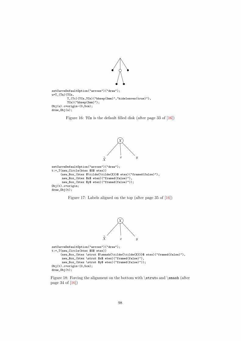
setCurveDefaultOption("arrows")("draw");
u=T_(Tn)(TCs,
T_(Tc)(TCs,TCs)("hbsep(5mm)","hideleaves(true)"),
TCs)("hbsep(5mm)");
Obj(u).c=origin-(0,5cm);
draw_Obj(u);
Figure 16: TCs is the default filled disk (after page 33 of [16])
˜Xx y
X
setCurveDefaultOption("arrows")("draw");
t:=_T(new_Circle(btex $X$ etex))
(new_Box_(btex $\tilde{\tilde{X}}$ etex)("framed(false)"),
new_Box_(btex $x$ etex)("framed(false)"),
new_Box_(btex $y$ etex)("framed(false)"));
Obj(t).c=origin;
draw_Obj(t);
Figure 17: Labels aligned on the top (after page 35 of [16])
˜X x y
X
setCurveDefaultOption("arrows")("draw");
t:=_T(new_Circle(btex $X$ etex))
(new_Box_(btex \strut $\smash{\tilde{\tilde{X}}}$ etex)("framed(false)"),
new_Box_(btex \strut $x$ etex)("framed(false)"),
new_Box_(btex \strut $y$ etex)("framed(false)"));
Obj(t).c=origin-(0,5cm);
draw_Obj(t);
Figure 18: Forcing the alignment on the bottom with \struts and \smash (afterpage 34 of [16])
98
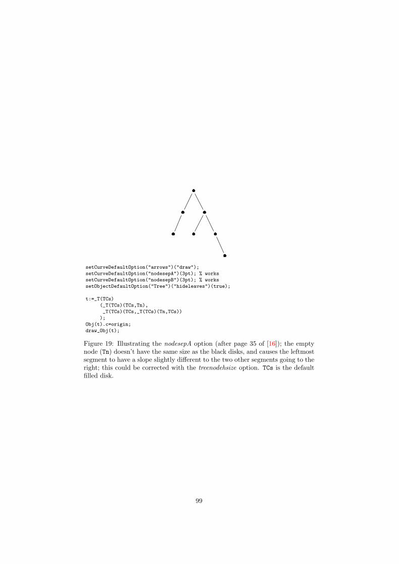
setCurveDefaultOption("arrows")("draw");
setCurveDefaultOption("nodesepA")(3pt); % works
setCurveDefaultOption("nodesepB")(3pt); % works
setObjectDefaultOption("Tree")("hideleaves")(true);
t:=_T(TCs)
(_T(TCs)(TCs,Tn),
_T(TCs)(TCs,_T(TCs)(Tn,TCs))
);
Obj(t).c=origin;
draw_Obj(t);
Figure 19: Illustrating the nodesepA option (after page 35 of [16]); the emptynode (Tn) doesn’t have the same size as the black disks, and causes the leftmostsegment to have a slope slightly different to the two other segments going to theright; this could be corrected with the treenodehsize option. TCs is the defaultfilled disk.
99

+
++ +
def Tdot(expr p)=
new_Circle_(p)("circmargin(-.2mm)")
enddef;
def Toplus=
Tdot(btex $+$ etex)
enddef;
setCurveDefaultOption("arrows")("draw");
setObjectDefaultOption("Tree")("hideleaves")(true);
setCurveDefaultOption("nodesepA")(3pt);
setCurveDefaultOption("nodesepB")(3pt);
setObjectDefaultOption("Tree")("Ualign")("center");
setObjectDefaultOption("Tree")("Lalign")("center");
setObjectDefaultOption("Tree")("hbsep")(5mm);
setObjectDefaultOption("Tree")("vbsep")(5mm);
setObjectDefaultOption("Tree")("hsep")(2cm);
setObjectDefaultOption("Tree")("vsep")(2cm);
t:=T_(Tc_(1.5mm))
(T_(Tc_(1.5mm))(Toplus,Toplus)("treemode(L)"),Toplus,Toplus)
("treemode(U)");
Obj(t).c=origin;
draw_Obj(t);
Figure 20: A tree with two different directions (after page 37 of [16])
B root
A1 A2
root
setCurveDefaultOption("arrows")("draw");
setObjectDefaultOption("Tree")("hsep")(1cm);
setObjectDefaultOption("Tree")("vsep")(1cm);
% we draw two trees which share a root node:
t:=T_(new_Circle(btex root etex))(Tr_(btex B etex))("treemode(L)");
Obj(t).c=origin;
u:=_T(obj(Obj(t).root))(Tr_(btex A1 etex),Tr_(btex A2 etex));
draw_Obj(t);
draw_Obj(u);
Figure 21: Two trees sharing the same root node (after page 37 of [16]); thereare two draw Obj commands to draw them, and actually the root will be drawntwice. The u tree is automatically positionned, because its root is already setin the first tree.
100
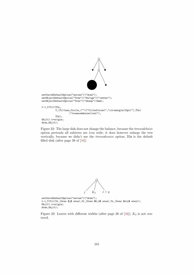
setCurveDefaultOption("arrows")("draw");
setObjectDefaultOption("Tree")("Dalign")("center");
setObjectDefaultOption("Tree")("hbsep")(5mm);
t:=_T(Tc)(TCs,
T_(Tc)(new_Circle_("")("filled(true)","circmargin(15pt)"),TCs)
("treenodehsize(1cm)"),
TCs);
Obj(t).c=origin;
draw_Obj(t);
Figure 22: The large disk does not change the balance, because the treenodehsizeoption pretends all subtrees are 1cm wide; it does however enlarge the treevertically, because we didn’t use the treenodevsize option; TCs is the defaultfilled disk (after page 38 of [16])
j K4 x > y
setCurveDefaultOption("arrows")("draw");
t:=_T(Tc)(Tr_(btex $j$ etex),Tr_(btex $K_4$ etex),Tr_(btex $x>y$ etex));
Obj(t).c=origin;
draw_Obj(t);
Figure 23: Leaves with different widths (after page 38 of [16]); K4 is not cen-tered.
101
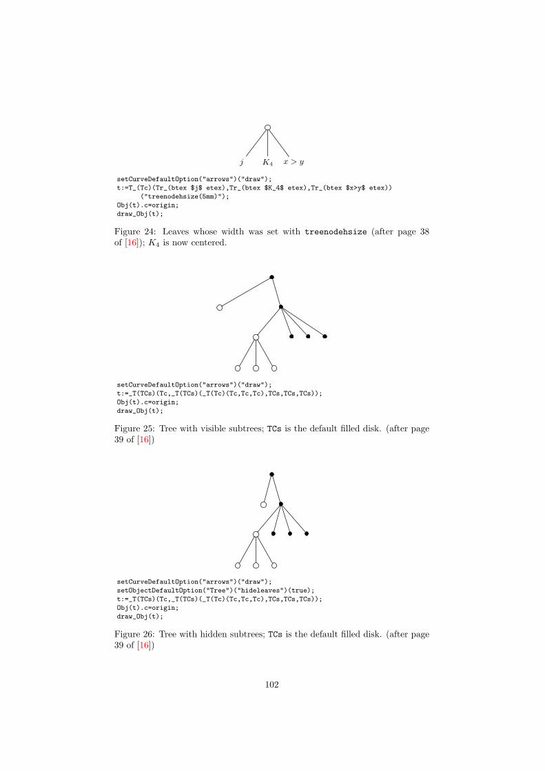
j K4 x > y
setCurveDefaultOption("arrows")("draw");
t:=T_(Tc)(Tr_(btex $j$ etex),Tr_(btex $K_4$ etex),Tr_(btex $x>y$ etex))
("treenodehsize(5mm)");
Obj(t).c=origin;
draw_Obj(t);
Figure 24: Leaves whose width was set with treenodehsize (after page 38of [16]); K4 is now centered.
setCurveDefaultOption("arrows")("draw");
t:=_T(TCs)(Tc,_T(TCs)(_T(Tc)(Tc,Tc,Tc),TCs,TCs,TCs));
Obj(t).c=origin;
draw_Obj(t);
Figure 25: Tree with visible subtrees; TCs is the default filled disk. (after page39 of [16])
setCurveDefaultOption("arrows")("draw");
setObjectDefaultOption("Tree")("hideleaves")(true);
t:=_T(TCs)(Tc,_T(TCs)(_T(Tc)(Tc,Tc,Tc),TCs,TCs,TCs));
Obj(t).c=origin;
draw_Obj(t);
Figure 26: Tree with hidden subtrees; TCs is the default filled disk. (after page39 of [16])
102
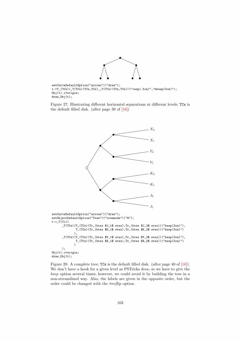
setCurveDefaultOption("arrows")("draw");
t:=T_(TCs)(_T(TCs)(TCs,TCs),_T(TCs)(TCs,TCs))("vsep(.5cm)","hbsep(2cm)");
Obj(t).c=origin;
draw_Obj(t);
Figure 27: Illustrating different horizontal separations at different levels; TCs isthe default filled disk. (after page 39 of [16])
J1
J2
K1
K2
Y1
Y2
X1
X2
setCurveDefaultOption("arrows")("draw");
setObjectDefaultOption("Tree")("treemode")("R");
t:=_T(Tc)(
_T(TCs)(T_(TCs)(Tr_(btex $J_1$ etex),Tr_(btex $J_2$ etex))("hsep(3cm)"),
T_(TCs)(Tr_(btex $K_1$ etex),Tr_(btex $K_2$ etex))("hsep(3cm)")
),
_T(TCs)(T_(TCs)(Tr_(btex $Y_1$ etex),Tr_(btex $Y_2$ etex))("hsep(3cm)"),
T_(TCs)(Tr_(btex $X_1$ etex),Tr_(btex $X_2$ etex))("hsep(3cm)")
)
);
Obj(t).c=origin;
draw_Obj(t);
Figure 28: A complete tree; TCs is the default filled disk. (after page 40 of [16]).We don’t have a hook for a given level as PSTricks does, so we have to give thehsep option several times; however, we could avoid it by building the tree in anon-streamlined way. Also, the labels are given in the opposite order, but theorder could be changed with the treeflip option.
103
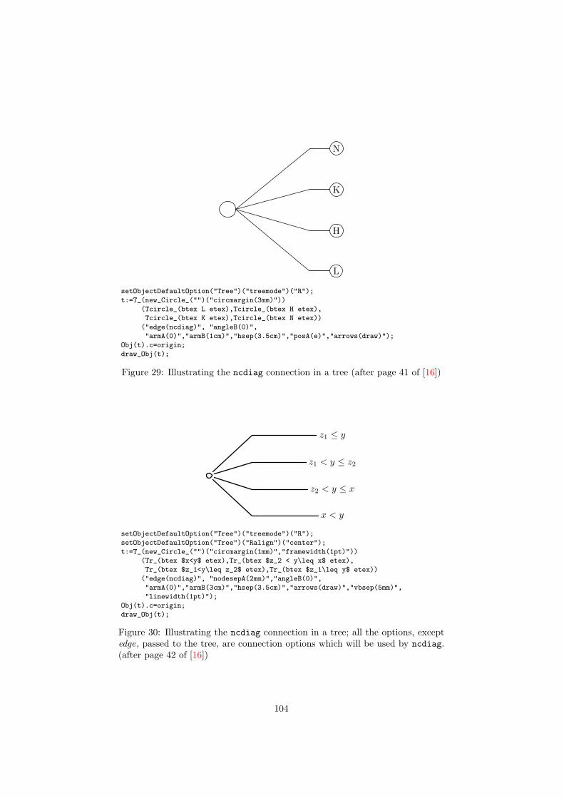
L
H
K
N
setObjectDefaultOption("Tree")("treemode")("R");
t:=T_(new_Circle_("")("circmargin(3mm)"))
(Tcircle_(btex L etex),Tcircle_(btex H etex),
Tcircle_(btex K etex),Tcircle_(btex N etex))
("edge(ncdiag)", "angleB(0)",
"armA(0)","armB(1cm)","hsep(3.5cm)","posA(e)","arrows(draw)");
Obj(t).c=origin;
draw_Obj(t);
Figure 29: Illustrating the ncdiag connection in a tree (after page 41 of [16])
x < y
z2 < y ≤ x
z1 < y ≤ z2
z1 ≤ y
setObjectDefaultOption("Tree")("treemode")("R");
setObjectDefaultOption("Tree")("Ralign")("center");
t:=T_(new_Circle_("")("circmargin(1mm)","framewidth(1pt)"))
(Tr_(btex $x<y$ etex),Tr_(btex $z_2 < y\leq x$ etex),
Tr_(btex $z_1<y\leq z_2$ etex),Tr_(btex $z_1\leq y$ etex))
("edge(ncdiag)", "nodesepA(2mm)","angleB(0)",
"armA(0)","armB(3cm)","hsep(3.5cm)","arrows(draw)","vbsep(5mm)",
"linewidth(1pt)");
Obj(t).c=origin;
draw_Obj(t);
Figure 30: Illustrating the ncdiag connection in a tree; all the options, exceptedge, passed to the tree, are connection options which will be used by ncdiag.(after page 42 of [16])
104

setObjectDefaultOption("Tree")("treemode")("U");
setObjectDefaultOption("Tree")("hbsep")(5mm);
setObjectDefaultOption("Tree")("hideleaves")(true);
setCurveDefaultOption("arrows")("draw");
t:=_T(Tc)(TCs,_T(Tc)(TCs,TCs),TCs);
% changes to the edges:
setTreeEdge(Obj(t))(1)(linestyle)("dashed evenly");
setTreeEdge(treepos(Obj(t))(2))(1)(linestyle)("dashed evenly");
Obj(t).c=origin;
draw_Obj(t);
Figure 31: Changing the style of connections with setTreeEdge (after page 42of [16])
nature
setCurveDefaultOption("arrows")("draw");
setCurveDefaultOption("nodesepA")(2mm);
setCurveDefaultOption("nodesepB")(2mm);
t:=_T(Toval_(btex nature etex))
(_T(new_Circle_("")("circmargin(1mm)","name(top)"))(TCs,TCs),
_T(new_Circle_("")("circmargin(1mm)","name(bot)"))(TCs,TCs));
Obj(t).c=origin;
ncline.Obj(t)("top")("bot")
"nodesepA(0)","nodesepB(0)","linestyle(dashed evenly)";
draw_Obj(t);
Figure 32: Connecting two named nodes in a tree (after page 43 of [16]); thename option is used to give names to streamlined objects, and these namesare then used in the ncline connection command; TC is a filled circle of radius1mm.
105
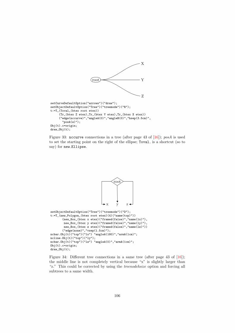
Z
Y
X
root
setCurveDefaultOption("arrows")("draw");
setObjectDefaultOption("Tree")("treemode")("R");
t:=T_(Toval_(btex root etex))
(Tr_(btex Z etex),Tr_(btex Y etex),Tr_(btex X etex))
("edge(nccurve)","angleA(0)","angleB(0)","hsep(3.5cm)",
"posA(e)");
Obj(t).c=origin;
draw_Obj(t);
Figure 33: nccurve connections in a tree (after page 43 of [16]); posA is usedto set the starting point on the right of the ellipse; Toval is a shortcut (so tosay) for new Ellipse.
x y z
root
setObjectDefaultOption("Tree")("treemode")("D");
t:=T_(new_Polygon_(btex root etex)(4)("name(top)"))
(new_Box_(btex x etex)("framed(false)","name(lx)"),
new_Box_(btex y etex)("framed(false)","name(ly)"),
new_Box_(btex z etex)("framed(false)","name(lz)"))
("edge(none)","vsep(1.5cm)");
ncbar.Obj(t)("top")("lx") "angleA(180)","armA(1cm)";
ncline.Obj(t)("top")("ly");
ncbar.Obj(t)("top")("lz") "angleA(0)","armA(1cm)";
Obj(t).c=origin;
draw_Obj(t);
Figure 34: Different tree connections in a same tree (after page 43 of [16]);the middle line is not completely vertical because “x” is slightly larger than“z.” This could be corrected by using the treenodehsize option and forcing allsubtrees to a same width.
106
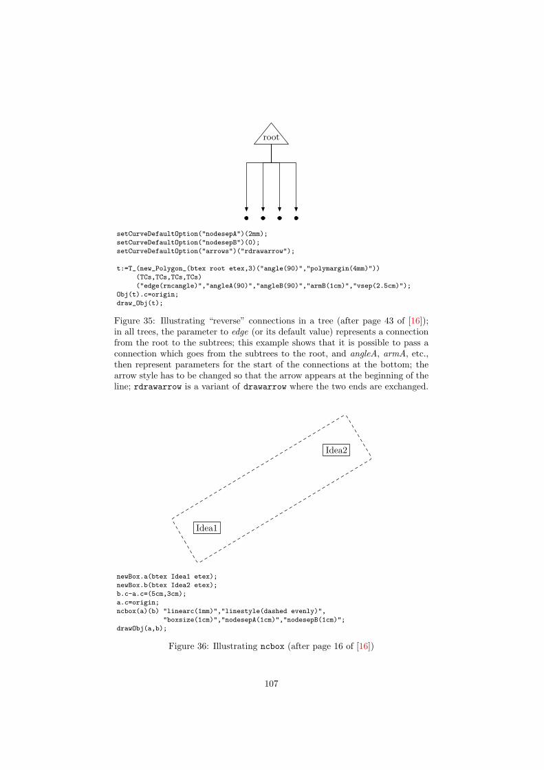
root
setCurveDefaultOption("nodesepA")(2mm);
setCurveDefaultOption("nodesepB")(0);
setCurveDefaultOption("arrows")("rdrawarrow");
t:=T_(new_Polygon_(btex root etex,3)("angle(90)","polymargin(4mm)"))
(TCs,TCs,TCs,TCs)
("edge(rncangle)","angleA(90)","angleB(90)","armB(1cm)","vsep(2.5cm)");
Obj(t).c=origin;
draw_Obj(t);
Figure 35: Illustrating “reverse” connections in a tree (after page 43 of [16]);in all trees, the parameter to edge (or its default value) represents a connectionfrom the root to the subtrees; this example shows that it is possible to pass aconnection which goes from the subtrees to the root, and angleA, armA, etc.,then represent parameters for the start of the connections at the bottom; thearrow style has to be changed so that the arrow appears at the beginning of theline; rdrawarrow is a variant of drawarrow where the two ends are exchanged.
Idea1
Idea2
newBox.a(btex Idea1 etex);
newBox.b(btex Idea2 etex);
b.c-a.c=(5cm,3cm);
a.c=origin;
ncbox(a)(b) "linearc(1mm)","linestyle(dashed evenly)",
"boxsize(1cm)","nodesepA(1cm)","nodesepB(1cm)";
drawObj(a,b);
Figure 36: Illustrating ncbox (after page 16 of [16])
107

Idea1
Idea2
newBox.a(btex Idea1 etex);
newBox.b(btex Idea2 etex);
b.c-a.c=(5cm,3cm);
a.c=origin;
ncarcbox(a)(b) "doubleline(true)",
"linestyle(dashed evenly)",
"boxsize(7mm)","nodesepA(1cm)","nodesepB(1cm)","arcangleA(-50)";
drawObj(a,b);
Figure 37: Illustrating ncarcbox (after page 16 of [16])
108
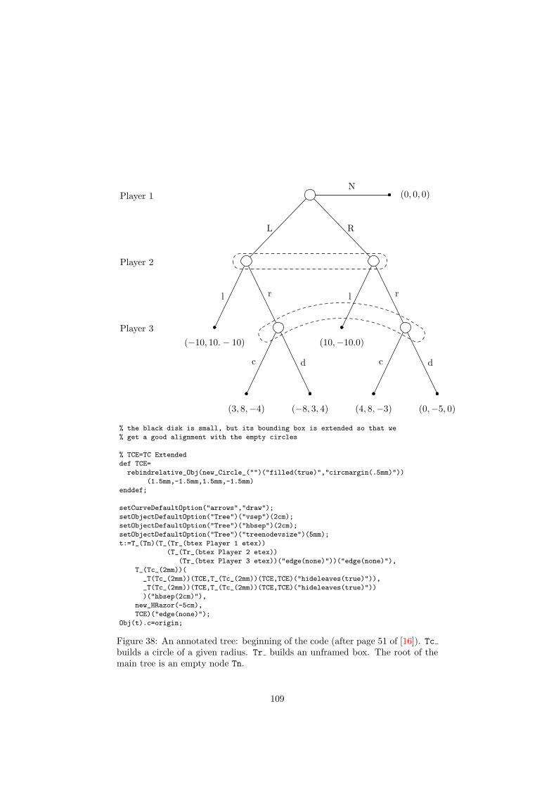
Player 3
Player 2
Player 1
(−10, 10.− 10)
(3, 8,−4) (−8, 3, 4)
c d
l r
(10,−10.0)
(4, 8,−3) (0,−5, 0)
c d
l r
L R
(0, 0, 0)N
% the black disk is small, but its bounding box is extended so that we
% get a good alignment with the empty circles
% TCE=TC Extended
def TCE=
rebindrelative_Obj(new_Circle_("")("filled(true)","circmargin(.5mm)"))
(1.5mm,-1.5mm,1.5mm,-1.5mm)
enddef;
setCurveDefaultOption("arrows","draw");
setObjectDefaultOption("Tree")("vsep")(2cm);
setObjectDefaultOption("Tree")("hbsep")(2cm);
setObjectDefaultOption("Tree")("treenodevsize")(5mm);
t:=T_(Tn)(T_(Tr_(btex Player 1 etex))
(T_(Tr_(btex Player 2 etex))
(Tr_(btex Player 3 etex))("edge(none)"))("edge(none)"),
T_(Tc_(2mm))(
_T(Tc_(2mm))(TCE,T_(Tc_(2mm))(TCE,TCE)("hideleaves(true)")),
_T(Tc_(2mm))(TCE,T_(Tc_(2mm))(TCE,TCE)("hideleaves(true)"))
)("hbsep(2cm)"),
new_HRazor(-5cm),
TCE)("edge(none)");
Obj(t).c=origin;
Figure 38: An annotated tree: beginning of the code (after page 51 of [16]). Tcbuilds a circle of a given radius. Tr builds an unframed box. The root of themain tree is an empty node Tn.
109
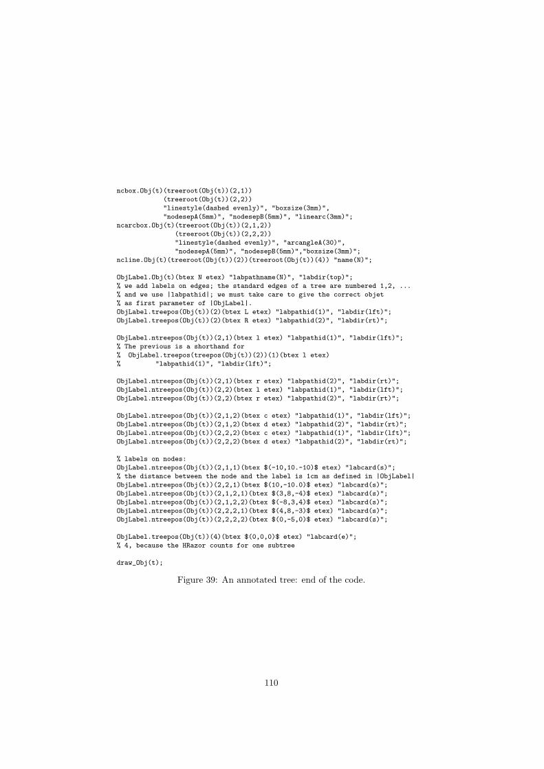
ncbox.Obj(t)(treeroot(Obj(t))(2,1))
(treeroot(Obj(t))(2,2))
"linestyle(dashed evenly)", "boxsize(3mm)",
"nodesepA(5mm)", "nodesepB(5mm)", "linearc(3mm)";
ncarcbox.Obj(t)(treeroot(Obj(t))(2,1,2))
(treeroot(Obj(t))(2,2,2))
"linestyle(dashed evenly)", "arcangleA(30)",
"nodesepA(5mm)", "nodesepB(5mm)","boxsize(3mm)";
ncline.Obj(t)(treeroot(Obj(t))(2))(treeroot(Obj(t))(4)) "name(N)";
ObjLabel.Obj(t)(btex N etex) "labpathname(N)", "labdir(top)";
% we add labels on edges; the standard edges of a tree are numbered 1,2, ...
% and we use |labpathid|; we must take care to give the correct objet
% as first parameter of |ObjLabel|.
ObjLabel.treepos(Obj(t))(2)(btex L etex) "labpathid(1)", "labdir(lft)";
ObjLabel.treepos(Obj(t))(2)(btex R etex) "labpathid(2)", "labdir(rt)";
ObjLabel.ntreepos(Obj(t))(2,1)(btex l etex) "labpathid(1)", "labdir(lft)";
% The previous is a shorthand for
% ObjLabel.treepos(treepos(Obj(t))(2))(1)(btex l etex)
% "labpathid(1)", "labdir(lft)";
ObjLabel.ntreepos(Obj(t))(2,1)(btex r etex) "labpathid(2)", "labdir(rt)";
ObjLabel.ntreepos(Obj(t))(2,2)(btex l etex) "labpathid(1)", "labdir(lft)";
ObjLabel.ntreepos(Obj(t))(2,2)(btex r etex) "labpathid(2)", "labdir(rt)";
ObjLabel.ntreepos(Obj(t))(2,1,2)(btex c etex) "labpathid(1)", "labdir(lft)";
ObjLabel.ntreepos(Obj(t))(2,1,2)(btex d etex) "labpathid(2)", "labdir(rt)";
ObjLabel.ntreepos(Obj(t))(2,2,2)(btex c etex) "labpathid(1)", "labdir(lft)";
ObjLabel.ntreepos(Obj(t))(2,2,2)(btex d etex) "labpathid(2)", "labdir(rt)";
% labels on nodes:
ObjLabel.ntreepos(Obj(t))(2,1,1)(btex $(-10,10.-10)$ etex) "labcard(s)";
% the distance between the node and the label is 1cm as defined in |ObjLabel|
ObjLabel.ntreepos(Obj(t))(2,2,1)(btex $(10,-10.0)$ etex) "labcard(s)";
ObjLabel.ntreepos(Obj(t))(2,1,2,1)(btex $(3,8,-4)$ etex) "labcard(s)";
ObjLabel.ntreepos(Obj(t))(2,1,2,2)(btex $(-8,3,4)$ etex) "labcard(s)";
ObjLabel.ntreepos(Obj(t))(2,2,2,1)(btex $(4,8,-3)$ etex) "labcard(s)";
ObjLabel.ntreepos(Obj(t))(2,2,2,2)(btex $(0,-5,0)$ etex) "labcard(s)";
ObjLabel.treepos(Obj(t))(4)(btex $(0,0,0)$ etex) "labcard(e)";
% 4, because the HRazor counts for one subtree
draw_Obj(t);
Figure 39: An annotated tree: end of the code.
110
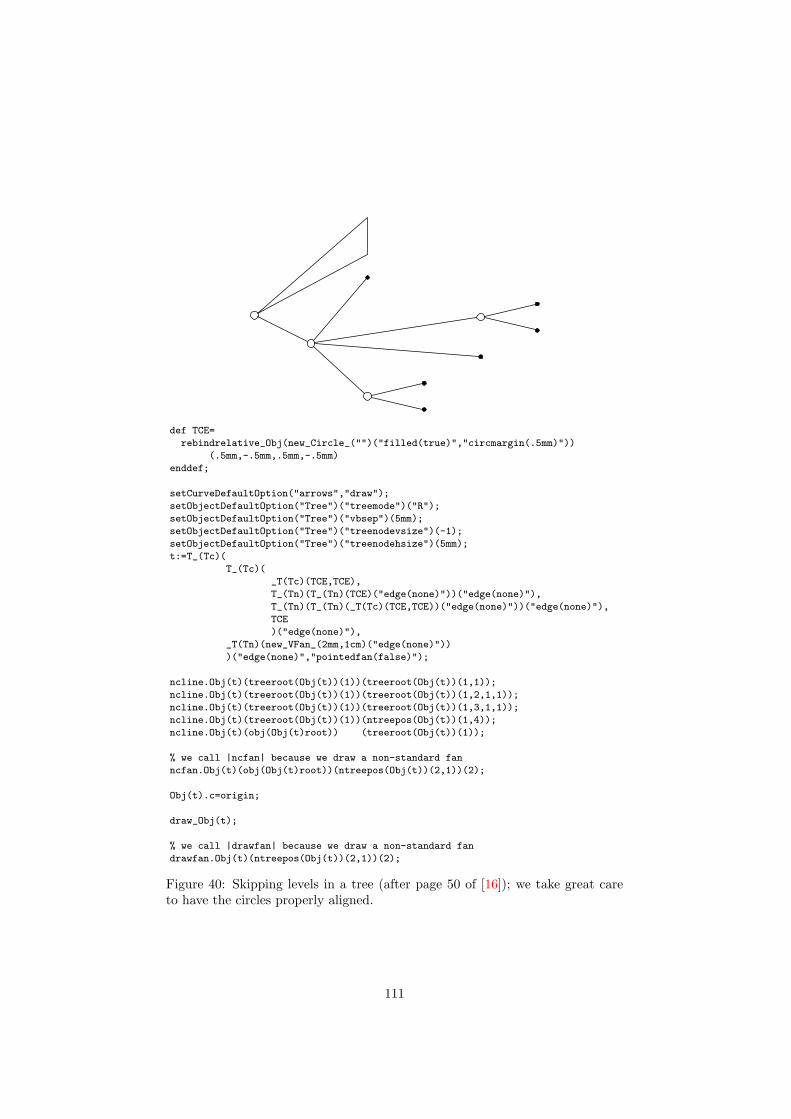
def TCE=
rebindrelative_Obj(new_Circle_("")("filled(true)","circmargin(.5mm)"))
(.5mm,-.5mm,.5mm,-.5mm)
enddef;
setCurveDefaultOption("arrows","draw");
setObjectDefaultOption("Tree")("treemode")("R");
setObjectDefaultOption("Tree")("vbsep")(5mm);
setObjectDefaultOption("Tree")("treenodevsize")(-1);
setObjectDefaultOption("Tree")("treenodehsize")(5mm);
t:=T_(Tc)(
T_(Tc)(
_T(Tc)(TCE,TCE),
T_(Tn)(T_(Tn)(TCE)("edge(none)"))("edge(none)"),
T_(Tn)(T_(Tn)(_T(Tc)(TCE,TCE))("edge(none)"))("edge(none)"),
TCE
)("edge(none)"),
_T(Tn)(new_VFan_(2mm,1cm)("edge(none)"))
)("edge(none)","pointedfan(false)");
ncline.Obj(t)(treeroot(Obj(t))(1))(treeroot(Obj(t))(1,1));
ncline.Obj(t)(treeroot(Obj(t))(1))(treeroot(Obj(t))(1,2,1,1));
ncline.Obj(t)(treeroot(Obj(t))(1))(treeroot(Obj(t))(1,3,1,1));
ncline.Obj(t)(treeroot(Obj(t))(1))(ntreepos(Obj(t))(1,4));
ncline.Obj(t)(obj(Obj(t)root)) (treeroot(Obj(t))(1));
% we call |ncfan| because we draw a non-standard fan
ncfan.Obj(t)(obj(Obj(t)root))(ntreepos(Obj(t))(2,1))(2);
Obj(t).c=origin;
draw_Obj(t);
% we call |drawfan| because we draw a non-standard fan
drawfan.Obj(t)(ntreepos(Obj(t))(2,1))(2);
Figure 40: Skipping levels in a tree (after page 50 of [16]); we take great careto have the circles properly aligned.
111
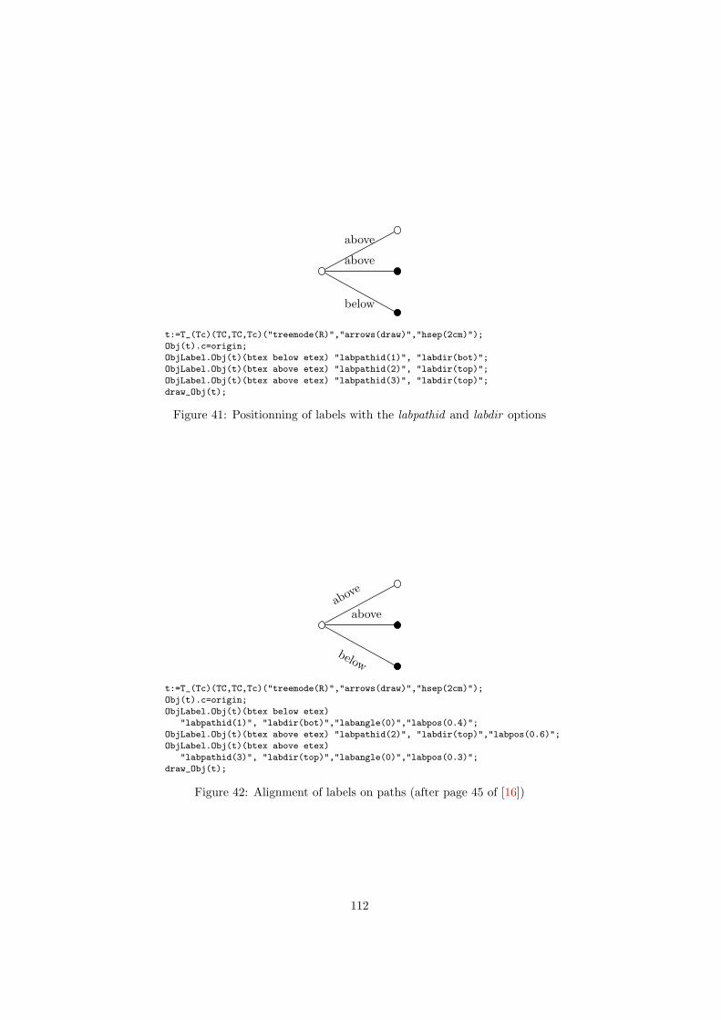
below
above
above
t:=T_(Tc)(TC,TC,Tc)("treemode(R)","arrows(draw)","hsep(2cm)");
Obj(t).c=origin;
ObjLabel.Obj(t)(btex below etex) "labpathid(1)", "labdir(bot)";
ObjLabel.Obj(t)(btex above etex) "labpathid(2)", "labdir(top)";
ObjLabel.Obj(t)(btex above etex) "labpathid(3)", "labdir(top)";
draw_Obj(t);
Figure 41: Positionning of labels with the labpathid and labdir options
below
aboveabove
t:=T_(Tc)(TC,TC,Tc)("treemode(R)","arrows(draw)","hsep(2cm)");
Obj(t).c=origin;
ObjLabel.Obj(t)(btex below etex)
"labpathid(1)", "labdir(bot)","labangle(0)","labpos(0.4)";
ObjLabel.Obj(t)(btex above etex) "labpathid(2)", "labdir(top)","labpos(0.6)";
ObjLabel.Obj(t)(btex above etex)
"labpathid(3)", "labdir(top)","labangle(0)","labpos(0.3)";
draw_Obj(t);
Figure 42: Alignment of labels on paths (after page 45 of [16])
112

Double box with green shadow
hexagon
a b
c
c
a
b
c
newBox.a("a");
newEllipse.b("b");
newEllipse.c("c") "filled(true)", "fillcolor(red)","picturecolor(green)",
"framecolor(blue)","framewidth(2pt)";
newTree.t(c)(a,b) "linecolor((1,1,0))";
newBox.aa(t) "filled(true)", "fillcolor((0,1,1))","rbox_radius(2mm)";
aa.c=origin;
newHexagon.xa("hexagon") "fit(false)","filled(true)","fillcolor((1,0,1))";
newEllipse.xc("c") "filled(true)", "fillcolor(red)","picturecolor(green)",
"framecolor(blue)","framewidth(2pt)";
newTree.xt(xc)(xa,aa) "linecolor((1,1,0))";
newCircle.xaa(xt) "filled(true)", "fillcolor((.6,.8,.5))";
newDBox.db(btex Double box with green shadow etex)
"shadow(true)", "shadowcolor(green)",
"filled(true)","fillcolor(blue)","picturecolor((1,1,0))";
newTree.nt(xaa)(db);
drawObj(nt);
nccoil(xc)(db) "angleA(0)","angleB(180)",
"coilwidth(5mm)","linetension(0.8)","linecolor(red)",
"doubleline(true)","posB(e)";
duplicateObj(dt,aa);
reflectObj(dt,origin,up);
slantObj(dt,.5);
rotateObj(dt,30);
dt.c=nt.c-(6cm,-1cm);
drawObj(dt);
nczigzag(a)(treepos(obj(dt.sub))(1))
"angleA(-120)","coilwidth(7mm)","linecolor(.5green)","linearc(1mm)",
"border(2pt)";
Figure 43: Cover example. The standard Tree class draws the paths before thecomponents, because the junction with objects are then better, in case the nodeframes are of a different color than the paths. This is why we drew the coil afterthe main object. As a consequence, the coil is not part of the object and won’tmove with it. It is possible to see the path and still attach it to the object bymodifying the draw function of the object.
113
8 Class builder manual
8.1 Components of a class
A class 〈C 〉 has a name which can’t begin or end with _. An object of such aclass is defined by a constructor and various other functions are associated toit.
8.1.1 Constructor
The definition of a class 〈C 〉 is:
vardef new〈C 〉@#〈parameters〉 text options =ExecuteOptions(@#)(options);assignObj(@#,"〈C 〉");StandardInterface;〈variables〉〈code〉〈standard paths〉StandardTies;
enddef;
This constructor takes parameters, for instance a list of objects. It alsotakes an optional list of options. The options are evaluated by ExecuteOptionsand some bookkeeping is done when assignObj is called. StandardInterfacedefines the points and equations corresponding to the standard interface.
〈variables〉 is a list of declarations of variables. These variables can be or-dinary metapost variables (and save should be used to keep them local tothe constructor) or object attributes. The following simple object attributedeclarations are recognized:
• ObjNumeric 〈numlist〉: declares each element of 〈numlist〉 as a numericfor the current object; for instance: ObjNumeric a,b. These values donot change when a linear transformation is applied to the object. A nu-merical value can be set in a constructor with setNumeric which takesan ObjNumeric name and a numerical value as parameters, for instance:setNumeric(num)(n). These numerical values can be used in the objectequations by prefixing them with @#.
• ObjPoint 〈pointlist〉: declares each element of 〈pointlist〉 as a point forthe current object; for instance: ObjPoint a,b. These points move whenthe object is transformed. They can be used in the object equations byprefixing them with @#.
• ObjPair 〈pairlist〉: declares each element of 〈pairlist〉 as a pair for thecurrent object; for instance: ObjPair a,b. A pair value can be set withsetPair which takes an ObjPair name and a pair value as parameters:setPair(p)(v). These pairs do not move when the object is transformed.They are like constant points. They can be used in the object equationsby prefixing them with @#.
114

• ObjPicture 〈piclist〉: declares each element of 〈piclist〉 as a picture for thecurrent object; for instance: ObjPicture a,b. A picture can be set withsetPicture which takes an ObjPicture name and a picture as parame-ters: setPicture(pic)(p). To each picture 〈p〉, ObjPicture associates apoint 〈p.off 〉 which is the picture offset. The pictures can be used in theobject equations by prefixing them with @#.
• ObjColor, ObjBoolean, ObjString and ObjTransform are commands sim-ilar to ObjNumeric and ObjPair and they also have associated setColor,setBoolean, setString and setTransform commands.
• SubObject(〈name〉,〈object〉): declares 〈name〉 as a string containing thename of object 〈object〉; for instance, SubObject(root,theroot). Theseobjects can be referred to in the equations by calling obj on their nameprefixed with @#.
There is also an ObjPath command which defines standard paths. However,they must be defined in the 〈standardpaths〉 section, once all equations aredefined.
It is also possible to declare arrays with ObjColorArray, ObjBooleanArray,ObjNumericArray, ObjPointArray, ObjPairArray, ObjStringArray,ObjTransformArray and ObjSubArray.
These commands all have the same syntax. They take two parameters. Thefirst is the name of the array and the second is its size. The size of the array isstored in the subcomponent n_ of the array. For instance,
ObjSubArray(sb)(Nx*Ny);
declares the array sb of size Nx×Ny as part of the current object and the size isrecorded in sb.n . This array is an array of subobject names, that is, an array ofstrings. Arrays are numbered from 1. This is a convention in the duplicateObjfunction, and if you go beyond the boundaries or use non-integer indices, theduplication will forget things.
The metaobj source code has many examples of these commands.
〈code〉 is actually a list of strings representing equations. They are declaredwith ObjCode. These strings can be constructed using other variables or options.It is possible to embed low-level metapost code in these strings, and not onlyequations. The concatenation of these strings is executed when the object iscreated, and also when the object is reset (but this is an experimental andunsupported function). Usually one of the strings is StandardEquations. Theequations must represent linear constraints. For instance, it is not possible tospecify a rotation by an unknown angle.
In the 〈standardpaths〉 section, paths can be defined with ObjPath. Thiscommand takes a path and can be followed by options. Here is an example:
ObjPath(obj(@#suba).b{dir(60)}..obj(@#subb).b)"linecolor(green)";
Finally, StandardTies ties the subobjects to the main object.
115
8.1.2 Streamlined constructor
In order to be able to chain the objects, one should use “streamlined” versions ofthe constructors. They can be created with appropriate calls to the streamlinecommand. For instance, the streamlined versions of newPolygon are obtainedwith
streamline("Polygon")("(expr v,nsides)","(v,nsides)");
The parameters of streamline are explained in section 5.1.
8.1.3 Bounding path
Each class 〈C 〉 should have a Bpath〈C 〉 function defining the “bounding path.”This path is used for instance when connections are drawn between two objects.The function takes the name of the object as a parameter. This name can beused to access points, or options, etc.
Here is the corresponding function for the Polygon class:
def BpathPolygon(suffix n)=(for i:=1 upto n.po.n_: n.po[i]--endfor cycle)
enddef;
8.1.4 Drawing function
Each class 〈C 〉 should also define a draw〈C 〉 function defining the way a 〈C 〉object is drawn. The corresponding function for the Polygon class is:
def drawPolygon(suffix n)=drawFramedOrFilledObject_(n);drawPictureOrObject(n);drawMemorizedPaths_(n);
enddef;
This function specifies that in order to draw a Polygon, the frame shouldbe drawn first (possibly filled), then the contents, then additional memorizedpaths. Memorized paths are typically paths added with the connection com-mands (ncline, etc.).
8.1.5 Alternate constructors
Certain objects have alternate constructors, for instance for compatibility rea-sons with other packages.
metaobj defines the newPentagon constructor as a variant of newPolygon:
vardef newPentagon@#(expr v) text options=newPolygon@#(v,5) options;
enddef;
116

8.1.6 Additional functions
A class can have associated functions which make its code simpler. These func-tions can use all the functions defined in metaobj. One interesting functionthat can be used is the is〈C 〉 function which tests whether a given object be-longs to a class or not. For instance, one of the internal functions associated tothe Tree class is the following:
def TreeRootObj_(suffix sb)=(if isBB(sb): TreeRootObj_(obj(sb.sub))elseif isTree(sb): TreeRootObj_(obj(sb.root))else: sbfi
)enddef;
Given an object, this function unwraps all BB layers it may contain, andwhen it reaches a Tree object, it calls itself on its root (which can itself be aTree), and so on. Only when the object is neither a Tree, nor a BB wrap, doesthe function return the object itself.
These is〈C 〉 functions are defined automatically and do not need to bedefined by the user.
8.1.7 Option declarations
If the 〈C 〉 class uses options that are not yet part of metaobj, they should bedefined with one of the following commands:
• define local numeric option
• define local pair option
• define local string option
• define local color option
• define local boolean option
• define global numeric option
• define global pair option
• define global string option
• define global color option
• define global boolean option
The first five functions define local options, that is, options that are usedonly at the time of the constructor. The last functions define global options,that is, options that are used beyond the constructor, for instance when theobject is drawn. filled is such an option:
define_global_boolean_option("filled");
This option is used by many objects to decide whether the frame should befilled or not.
117

8.1.8 Default values for options
All the options should have a default value. This default value depends on theclass. It can be set with setObjectDefaultOption. For instance, here is howthe Tree class defines the default orientation of trees:
setObjectDefaultOption("Tree")("treemode")("D");
8.2 Design rules
Several metaobj functions assume that objects are rigid. Such objects can befloating, but the position of all the points should be determined by setting justone point.
It is of course possible to define objects with less constraints, but then theuser will have to define new functions to manipulate them.
When creating an object, the implementer should first try to define carac-teristic points which will be used to express the equations. These points shouldbe given names (different from those of the standard interfaces) and equationsbetween these points should be given. This will be sufficient for most objectswith straight lines.
The constraints on the points should be given as equations, never as as-signments (except for intermediate computations), otherwise objects might nolonger be floating.
For certain objects, the difficult part is to find the good equations. Forinstance, it is not that simple to find good equations for a triangle enclosinga rectangular box such as text. However, in many cases, the equations aresimple, but there are many different cases to consider, depending on the valuesof parameters and on the presence of certain subobjects.
Parameters should be introduced when necessary. These parameters shouldbe consistant with already existing parameters. When in doubt, new parameternames should be created.
Consider for instance the following object:
abcdefg
XXXXXXX
Here, we want a rectangular box where XXXXXXX (an object or a picture)is centered. In addition, we want some label at the top left. First, we shouldidentify the caracteristic points. It is natural to consider that the corners ofthe outer rectangle are those of the standard interface, and we need no morepoints for those. The corners of the inner XXXXXXX box are also those of itsstandard interface. For the top left label, we add three points: lsw, lse and
118
lne. The top label and the main XXXXXXX box will be parameters to thenew constructor.
Now, we have to decide the layout. Will XXXXXXX be centered, no matterthe size of the top left label or will it take the top left label into account? Theseare design decisions that must be taken. Let’s assume the top left label doesn’tinfluence the position of XXXXXXX. Let’s also assume that the size of the topleft rectangle is exactly that of the label. Finally, let’s assume there is a DXand DY clearance inside the box. This gives us the following equations (in plainlanguage):
let L=topleftlabelX=center boxM=main box
xpart(M.e-X.e)=xpart(X.w-M.w)=DXypart(M.n-X.n)=xpart(X.s-M.s)=DYM.nw=L.nwM.lsw=L.swM.lse=L.seM.lne=L.ne
and that’s it! Actually, we might even discard lsw, lse and lne, since they aregiven by L’s cardinal points.
Things get more complex when the object contains lines that are not straight.There are two cases: either it is easy to compute the line from certain points(this is done with the Circle and Ellipse constructors, for instance), or it iseasier to memorize the line as a path. This is what is done for round boxes(RBox).
9 Non-linear transformations on objects
The whole structure of an object is available and it is therefore possible to applyvarious transformations to an object. metaobj provides the standard meta-post linear transformations, but on objects: rotateObj, scaleObj, etc. Thereare however many other possible transformations. We will give a few exampleshere, by distinguishing two kinds of transformations.
9.1 Simple transformations which do not change the lay-out
The first kind of transformation does not change the positions of the points.These transformations only change various attributes. For instance, we mightwant to change the color of a frame when an object is duplicated, or maybechange some of the labels, without changing the layout.
9.1.1 Example 1: changing the frame color
Several attributes of an object are stored in fields that can easily be changed.This is for instance the case for the color of the frame. It is stored in theoption_framecolor_ field and it can be changed as shown here:
119
newEllipse.a(btex a framed text etex) "framecolor(red)";a.c=origin;drawObj(a);duplicateObj(b,a);b.option_framecolor_:=blue;b.c=origin-(0,2cm);drawObj(b);
9.1.2 Example 2: changing the content of a label
The label of a object such as an Ellipse is stored in its p field. We can givea new value to this field and the next time the object is drawn, the new valuewill be used. We have to be careful to center the label around the origin. Theframe of the object is unchanged and therefore it may be smaller or larger thanits contents.
newEllipse.a(btex bananas etex);a.c=origin;drawObj(a);duplicateObj(b,a);b.p:=btex apples etex;b.p:=b.p shifted -.5[urcorner(b.p),llcorner(b.p)];b.c=origin-(0,2cm);drawObj(b);
9.2 Transformations that change the layout
It is also possible to change the layout of an object, for instance by dismantlingit. Let’s for instance build a tree:
newBox.r(btex root etex);newBox.l1(btex leaf 1 etex);newBox.l2(btex leaf 2 etex);newBox.l3(btex leaf 3 etex);newTree.t(r)(l1,l2,l3)
"edge(nccoil)","coilarm(2mm)","coilwidth(3mm)";t.c=origin;drawObj(t);
One way to dismantle it is to make independant copies of each subobject:
duplicateObj(r2,obj(t.root));duplicateObj(l11,ntreepos(t)(1));duplicateObj(l12,ntreepos(t)(2));duplicateObj(l13,ntreepos(t)(3));
These objects can then be used to build a new tree:
newTree.t2(r2,l13,l12,l11) ;t2.c=origin-(0,4cm);drawObj(t2);
120

Another possibility is to “untie” the four components:
untieObj(obj(t.root));untieObj(ntreepos(t)(1));untieObj(ntreepos(t)(2));untieObj(ntreepos(t)(3));
The main object is now a wreck...But the components can be reused in a new tree:
newTree.t3(obj(t.root))(ntreepos(t)(1),ntreepos(t)(2),ntreepos(t)(3))"edge(nccoil)","coilarm(2mm)","coilwidth(5mm)","vsep(2cm)";
t3.c=origin-(0,7cm);drawObj(t3);
The three trees are shown in figure 44. The second and third trees wereobtained from the first tree.
leaf 1 leaf 2 leaf 3
root
leaf 3 leaf 2 leaf 1
root
leaf 1 leaf 2 leaf 3
root
Figure 44: Dismantling a tree
The possibilities are endless.
121
10 Comparison with other packages
10.1 Compatibility with boxes.mp
metaobj can be used instead of boxes.mp, but not together with boxes.mp.It contains most of the functionalities found in John Hobby’s boxes and rboxespackages. In particular, it uses the same syntax for accessing the cardinal pointsof an object or setting an object position.
The newBox constructor can be used in place of boxit and we have actu-ally redefined boxit to behave like newBox. Similarly, rboxit and circleithave been redefined to refer to newRBox (which is a variant of newBox) and tonewEllipse.
However, there is one important difference. In metaobj, when an object iscreated, it is rigid. Once the newBox constructor has been called, it is no longerpossible to (easily) change the values of dx and dy for instance. In the boxespackage, it is possible to define a box with a certain content, to put its centersomewhere after the call to boxit (this is also how it is done in metaobj), andthen to set the values of dx and dy. In metaobj, these values must be givenwhen newBox is called.
Nevertheless, it should be possible to reuse most of the figures written forthe boxes package with metaobj.
10.2 fancybox package
The fancybox package provides several ways to frame a box:
• \shadowbox : this can be achieved in metaobj with a Box and the shadowoption;
• \ovalbox, \Ovalbox: these two frames can be achieved with a Box (orRBox), and the appropriate values for the corner radius and the thicknessof the lines;
• \doublebox: this command puts a double rectangular frame around anobject; it can be achieved in metaobj with a DBox object, except forthe fact that the two frames have the same thickness in metaobj; infancybox, they have different thicknesses; DBox could easily be extendedto take this into account.
10.3 PSTricks
metaobj is not compatible with PSTricks, but it includes many functionali-ties that are similar to those provided by PSTricks. Many option names wereborrowed from PSTricks and all the node connections were implemented inmetaobj.
Section 7.7 shows how many examples from the PSTricks documentation canbe rendered in metaobj. The metaobj code is lengthier than the correspond-ing PSTricks code, but one should really compare a high-level TEX descriptionof a metaobj graphics with PSTricks code, and both would be very similar.
122
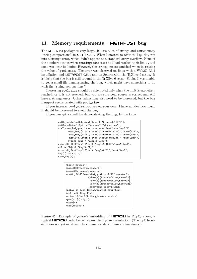
11 Memory requirements – metapost bug
The metaobj package is very large. It uses a lot of strings and causes many“string compactions” in metapost. When I started to write it, I quickly raninto a strange error, which didn’t appear as a standard array overflow. None ofthe numbers output when tracingstats is set to 1 had reached their limits, andnone was near its limits. However, the strange errors vanished when increasingthe value of pool_size. The error was observed on linux with a Web2C 7.3.1installation and metapost 0.641 and on Solaris with the TEXlive 5 setup. Itis likely that the bug is still around in the TEXlive 6 setup. So far, I was unableto get a small file demonstrating the bug, which might have something to dowith the “string compactions.”
Increasing pool_size should be attempted only when the limit is explicitelyreached, or it is not reached, but you are sure your source is correct and stillhave a strange error. Other values may also need to be increased, but the bugI suspect seems related with pool_size.
If you increase pool_size, you are on your own. I have no idea how muchit should be increased to avoid the bug.
If you can get a small file demonstrating the bug, let me know.
setObjectDefaultOption("Tree")("treemode")("D");
setCurveDefaultOption("arrows")("drawarrow");
t:=T_(new_Polygon_(btex root etex)(4)("name(top)"))
(new_Box_(btex x etex)("framed(false)","name(lx)"),
new_Box_(btex y etex)("framed(false)","name(ly)"),
new_Box_(btex z etex)("framed(false)","name(lz)"))
("edge(none)","vsep(1.5cm)");
ncbar.Obj(t)("top")("lx") "angleA(180)","armA(1cm)";
ncline.Obj(t)("top")("ly");
ncbar.Obj(t)("top")("lz") "angleA(0)","armA(1cm)";
Obj(t).c=origin;
draw_Obj(t);
\begin{metaobj}
\mosetO{Tree}{treemode=D}
\mosetC{arrows=drawarrow}
\setObj{t}{\Tree{\Polygon{root}{4}[name=top]}
{\Box{x}[framed=false,name=lx],
\Box{y}[framed=false,name=ly],
\Box{z}[framed=false,name=lz]}
[edge=none,vsep=1.5cm]}
\ncbar[t]{top}{lx}[angleA=180,armA=1cm]
\ncline[t]{top}{ly}
\ncbar[t]{top}{lz}[angleA=0,armA=1cm]
\pos{t.c}{origin}
\draw{t}
\end{metaobj}
Figure 45: Example of possible embedding of metaobj in LATEX; above, atypical metaobj code; below, a possible TEX representation. (The TEX front-end does not yet exist and the commands shown here are imaginary.)
123
12 Using metaobj from within TEX
metapost code can be embedded in LATEX with the emp.sty package (onCTAN) [13]. It should therefore be possible to embed metaobj code, thoughthis was not tested.
It should also be possible to use metaobj within ConTEXt [3, 4] wheremetapost code is naturally included in the main TEX file.
However, if metaobj benefits from being embedded in LATEX or ConTEXtcode, it would benefit even more if a TEX layer were hiding the verbose syntaxof metaobj. No syntax for a TEX front-end to metaobj has been defined sofar, but an example of a possible syntax is the one provided by PSTricks. It ispossible to have both concise code, and to use metaobj behind the scenes. Forinstance, in the future, we might input metaobj code as shown on figure 45.
Conclusion
metaobj makes it possible to define and manipulate objects. The standardfunctions consider that the objects are rigid and can be combined in variousways. No matter how an object has been built, its structure is still easilyaccessible and open to introspection. This is an important feature which hasalmost been left aside in this manual.
It is of course easy to add new objects and we have only provided a few. Itis also easy for the programmer to write special packages manipulating specialgraphical formalisms, such as UML, etc.
It should also be possible to extend the concept of interface to other kindsof interfaces and to introduce objects that are not completely rigid. We havealready mentionned that it is possible to use the complete object structure toimplement tree layout algorithms. We could also have objects whose shapedepends on parameters and on their location in a drawing. More elaborateoperations could also be implemented if the history of an object was known.This is currently not the case, and causes limitations in certain experimentalfeatures such as the reset feature.
metaobj can be used as a replacement to boxes.mp and rboxes.mp, tofancybox.sty and to many features found in PSTricks. Several features ofmetaobj, for instance connections, can be used without a reference to objects.
metaobj was especially influenced by my earlier work on animations [14]where an object notion was introduced. The 3D objects were very primitive,but they provided many useful ideas. Several objects have been influenced fromtheir counterparts in various packages. This is especially true for rectangularand elliptic boxes. PSTricks provided many ideas and the connection func-tions are entirely borrowed from that package. However, only PSTricks’s userdocumentation was used, not the details of its implementation [18], though sim-ilarities can be observed. There has also been some work by Denis Girou onhigh-level objects in PSTricks [1], but this work is not really relevant to whatwe have done. Another work we didn’t use was Kristoffer Rose’s work on highlevel 2-dimensional graphics [15]. The proof tree class was influenced by a LATEXpackage I wrote in 1993 and which was never released.
There are several systems which share ideas with metaobj, though theydidn’t influence it. One is “Functional metapost” [11, 12], a system which
124

provides a Haskell layer to specify drawings more abstractly. The drawback ofthat approach is that one needs a Haskell compiler and of course one needs tolearn some of this language. Nevertheless, this work shares many ideas withmetaobj in that objects are built by applying functions to already existingstructures. Another functional approach to picture drawing is FPIC [7] whichuses the ML language. A very popular system with many similar ideas is theJava2D API [8]. It provides graphical objects which can be manipulated byvarious transformations and modified in various ways.
The syntax of metaobj is admittedly verbose, but it is hoped that a TEXinterface will be provided and that it will alleviate a lot of the user’s burden.
Acknowledgments
I thank Denis Girou for some explanations on PSTricks’ \ncdiag, \ncdiagg and\ncloop commands, Bogus law Jackowski for helping me to find again the quoteon the first page, and Damien Wyart for some comments. Several users havereported bugs which have now been corrected: Marc van Dongen and EckhartGuthohrlein.
125
References
[1] Denis Girou. Building high level objects in PSTricks, 1995. Slidespresented at TUG’95, St Petersburg (Florida), http://www.tug.org/applications/PSTricks/TUG95-PSTricks_4.ps.gz.
[2] Michel Goossens, Sebastian Rahtz, and Frank Mittelbach. The LATEXGraphics Companion: Illustrating documents with TEX and PostScript.Reading, MA: Addison-Wesley, 1997.
[3] Hans Hagen. ConTEXt: the manual, 2000. http://www.pragma-ade.com.
[4] Hans Hagen. MetaFun, 2000. http://www.pragma-ade.com.
[5] John D. Hobby. A User’s manual for MetaPost. Technical report, AT&TBell Laboratories, Murray Hill, New Jersey, 1992. Computing Science Tech-nical Report 162.
[6] Alan Hoenig. TEX Unbound: LATEX & TEX Strategies for Fonts, Graphics,& More. New York: Oxford University Press, 1998.
[7] Samuel N. Kamin and David Hyatt. A Special-Purpose Language forPicture-Drawing. In USENIX Conf. on Domain-specific Languages, SantaBarbara, pages 297–310, October 1997. http://www-sal.cs.uiuc.edu/~kamin/fpic.
[8] Jonathan Knudsen. Java 2D Graphics. O’Reilly & Associates, 1999.
[9] Donald E. Knuth. The metafontbook. Reading, MA: Addison-Wesley,1986.
[10] Donald E. Knuth. Digital Typography, volume 78 of CSLI Lecture Notes.CSLI, 1999.
[11] Joachim Korittky. Functional metapost. Eine Beschreibungsspra-che fur Grafiken, 1998. Diplomarbeit an der Rheinischen Friedrich-WilhelmsUniversitat Bonn. http://tex.loria.fr.
[12] Marco Kuhlmann. Functional metapost for LATEX, 2001. http://tex.loria.fr.
[13] Thorsten Ohl. EMP: Encapsulated metapost for LATEX, 1997. TechnischeHochschule Darmstadt. http://tex.loria.fr.
[14] Denis Roegel. Creating 3D animations with metapost. TUG-boat, 18(4):274–283, 1997. ftp://ftp.loria.fr/pub/ctan/graphics/metapost/macros/3d/tugboat/tb57roeg.pdf.
[15] Kristoffer Høgsbro Rose. “Very High Level 2-dimensional Graphics” withTEX and XY-pic. TUGboat, 18(3):151–158, 1997. http://www.tug.org/TUGboat/Articles/tb18-3/tb56rose.pdf.
[16] Timothy van Zandt. PSTree user’s guide, 1993. ftp://ftp.loria.fr/pub/ctan/obsolete/pstricks/beta.
126
[17] Timothy van Zandt. PSTricks: PostScript macros for Generic TEX; User’sGuide, 1993. http://tex.loria.fr.
[18] Timothy van Zandt and Denis Girou. Inside PSTricks. TUGboat, 15(3):239–248, 1994. http://www.tug.org/TUGboat/Articles/tb15-3/tb44tvz.ps.
127

Index
T (command), 79
addPath (command), 31, 38addPathVariables (command), 37, 38addStandardPath (command), 38, 39addUserPath (command), 38, 91align (class option), 36, 68–70angle (class option), 63angle (connection option), 42angleA (connection option), 41, 44–
47, 50, 107angleB (connection option), 41, 44–
47, 50arcangle (connection option), 42arcangleA (connection option), 41,
45, 51arcangleB (connection option), 41,
45, 51arm (connection option), 42armA (connection option), 41, 45–
48, 107armB (connection option), 41, 45–
49arrows (connection option), 38, 40,
41, 43assignObj (command), 12, 22, 114Assumption (class), 83Attributes
booleanarraylist , 57code , 57, 59colorarraylist , 57ctransform , 57, 59extra code , 57nsubobjties , 57numericarraylist , 57numericlist , 57pairarraylist , 57pairlist , 57picturearraylist , 57picturelist , 57pointarraylist , 57pointlist , 56, 57points in arrayslist , 57stringarraylist , 57subarraylist , 57sublist , 56, 57subobjties , 57, 58
transformarraylist , 57Axiom (class), 83
BB (class), 27, 90, 117booleanarraylist (attribute), 57border (connection option), 41bordercolor (connection option), 41Box (class), 7, 61, 62, 65, 83boxdepth (connection option), 41,
50boxheight (connection option), 41,
50boxit (command), 10boxsize (connection option), 41, 50BpathCircle (command), 39BpathEmptyBox (command), 28BpathObj (command), 28bracketit.expl (command), 91btex (command), 30
cdraw (connection option), 41, 42Circle (class), 81, 119circleit (command), 10circmargin (class option), 64, 65, 67Class options
align, 36, 68–70angle, 63circmargin, 64, 65, 67Dalign, 74, 80dx, 62, 65, 66, 69, 70, 72, 80,
85, 92dy, 62, 65, 66, 69, 70, 72, 80,
85, 92edge, 80, 82, 104, 107elementsize, 69, 70fanlinearc, 81, 82fanlinestyle, 81, 82fillcolor, 34, 60–67, 69, 70, 72,
80–82, 85, 92filled, 34, 37, 60–67, 69, 70, 72,
80, 82, 85, 92, 117fit, 31, 62–64, 66, 67flip, 69, 70framecolor, 34, 60–67, 69, 70,
72, 80, 85, 92framed, 31, 34, 36, 59–67, 69,
70, 72, 80, 85, 92
128

framestyle, 34, 60–67, 69, 70,72, 80, 85, 92
framewidth, 34, 60–67, 69, 70,72, 80, 85, 92
halign, 89, 92hbsep, 68, 69, 80hideleaves, 77, 78, 80, 81hsep, 66, 67, 80, 85, 92, 103Lalign, 80lenddx, 84, 85lrsep, 85lstartdx, 85matrixnodehsize, 92matrixnodevsize, 92name, 37, 40, 105picturecolor, 26, 62–67pointedfan, 81, 82polymargin, 63Ralign, 80rbox radius, 31, 62rotangle, 72rrsep, 85rule, 85shadow, 31, 34, 59–67, 69, 70,
72, 80, 85, 92shadowcolor, 34, 59–67, 69, 70,
72, 80, 85, 92treeflip, 76, 80, 103treemode, 36, 37, 80, 83, 85treenodehsize, 80, 99, 101, 106treenodevsize, 80, 101Ualign, 80valign, 89, 92vbsep, 70, 80vsep, 66, 67, 70, 80, 85, 92
ClassesAssumption, 83Axiom, 83BB, 27, 34, 90, 117Box, 7, 8, 30, 31, 38, 61, 62,
65–67, 81, 83, 122Circle, 64, 81, 119Conclusion, 83DBox, 65, 66, 122DEllipse, 66Ellipse, 63, 66, 119, 120, 122EmptyBox, 9, 27, 28, 32, 60, 61HBox, 67–70, 80HFan, 81HRazor, 60, 81
Matrix, 89, 90, 92Pentagon, 116Polygon, 7, 62, 63, 116PTree, 56, 73, 82–84PTreeL, 83PTreeR, 83RandomBox, 60RBox, 81, 119, 122RecursiveBox, 28, 29, 71Tree, 7, 8, 32, 36, 42, 73, 79,
81, 82, 90, 113, 117, 118VBox, 67, 69, 80VFan, 81VonKochFlake, 8, 72VRazor, 60, 81
clearObj (command), 18code (attribute), 57, 59coilarm (connection option), 42coilarmA (connection option), 41, 52coilarmB (connection option), 41, 52coilaspect (connection option), 41,
52coilheight (connection option), 41,
52coilinc (connection option), 41, 52coilwidth (connection option), 41, 52colorarraylist (attribute), 57Commands
T, 79addPath, 31, 38addPathVariables, 37, 38addStandardPath, 38, 39addUserPath, 38, 91assignObj, 12, 22, 114boxit, 10BpathCircle, 39BpathEmptyBox, 28BpathObj, 28bracketit.expl, 91btex, 30circleit, 10clearObj, 18define global boolean option, 117define global color option, 117define global numeric option, 117define global pair option, 117define global string option, 117define local boolean option, 117define local color option, 117define local numeric option, 117
129

define local pair option, 117define local string option, 117deleteMatrixElement.expl, 90deleteTreeElement.expl, 82draw, 16, 23, 40, 43draw Obj, 32, 100drawarrow, 40, 43, 107drawBox, 31, 38drawCircle, 39drawEmptyBox, 28drawFramedOrFilledObject , 28,
31drawMemorizedPaths , 30, 31,
38drawObj, 14, 16, 20, 28, 29, 32drawPicture, 26drawRecursiveBox, 29drawVonKochSide, 72duplicate Obj, 33duplicateObj, 18, 19, 33, 73, 115etex, 30ExecuteOptions, 28, 114extendObjDown, 34extendObjLeft, 34, 75extendObjRight, 34, 75, 76extendObjUp, 34find bot most, 29find lft most, 29find rt most, 29find top most, 29image, 5, 61label, 55matpos, 54mcangle, 54mcangles, 54mcarc, 54mcarcbox, 54mcbox, 54mccircle, 54mccoil, 54mccurve, 54mcdiag, 54mcdiagg, 54mcline, 40, 54mcloop, 54mczigzag, 54mpos, 54nb, 89ncangle, 46, 48ncangles, 46, 48
ncarc, 45, 51ncarcbox, 41, 50, 51, 108ncbar, 45, 93ncbox, 41, 50, 51, 107nccircle, 40, 50nccoil, 52nccurve, 38, 41, 44, 106ncdiag, 47, 48, 104ncdiagg, 48ncline, 38, 40, 42, 44, 55, 93,
105, 116ncloop, 41, 48nczigzag, 52new Box, 32new Ellipse, 106new Polygon , 33new Tree, 79new Tree , 81newobjstring , 18, 28, 56newRBox, 62newTree, 79ntreepos, 56Obj, 32, 40, 54obj, 18, 115ObjBoolean, 115ObjBooleanArray, 115ObjCode, 12, 22, 31, 115ObjColor, 115ObjColorArray, 115ObjLabel, 54, 55, 91ObjNumeric, 29, 114, 115ObjNumericArray, 115ObjPair, 114, 115ObjPairArray, 115ObjPath, 39, 115ObjPicture, 25, 31, 115ObjPoint, 12, 31, 59, 114ObjPointArray, 115ObjString, 115ObjStringArray, 115ObjSubArray, 115ObjTransform, 115ObjTransformArray, 115OptionValue, 37rdrawarrow, 40, 107rebindObj, 34rebindrelativeObj, 34, 75, 76rebindVisibleObj, 24, 27, 34, 79replaceMatrixElement.expl, 90replaceTreeElement.expl, 82
130

rncangle, 54rncangles, 54rncarc, 54rncarcbox, 54rncbar, 54rncbox, 54rnccoil, 54rnccurve, 54rncdiag, 54rncdiagg, 54rncline, 54rncloop, 54rnczigzag, 54rotate Obj, 33rotateObj, 11, 29, 33, 119scaleObj, 24, 79, 119setBoolean, 115setColor, 115setCurveDefaultOption, 40, 42setNumeric, 114setObjectDefaultOption, 118setPair, 114setPicture, 115setString, 115setTransform, 115setTreeEdge, 105show empty boxes, 59showObj, 56, 58StandardEquations, 115StandardInterface, 114StandardObjectOrPictureContain-
erSetup, 30StandardTies, 17, 18, 28, 115streamline, 32, 116SubObject, 17, 115suffixlist, 33suffixpar, 33T, 79T , 81TC, 65, 105Tc, 64TC , 65Tc , 65, 109tcangle, 54tcangles, 54tcarc, 54tcarcbox, 54tcbox, 54tccircle, 54tccurve, 54
tcdiag, 54tcdiagg, 54Tcircle , 64tcline, 40, 54tcloop, 54TCs, 65, 97–99, 101–103Tf, 62, 81Tn, 59, 99, 109Toval , 64, 106Tr , 62, 106, 109transformObj, 11treenodehsize, 102untieObj, 15, 35vardef, 8whatever, 12
Conclusion (class), 83Connection options
angle, 42angleA, 41, 44–47, 50, 107angleB, 41, 44–47, 50arcangle, 42arcangleA, 41, 45, 51arcangleB, 41, 45, 51arm, 42armA, 41, 45–48, 107armB, 41, 45–49arrows, 38, 40, 41, 43border, 41bordercolor, 41boxdepth, 41, 50boxheight, 41, 50boxsize, 41, 50cdraw, 41, 42coilarm, 42coilarmA, 41, 52coilarmB, 41, 52coilaspect, 41, 52coilheight, 41, 52coilinc, 41, 52coilwidth, 41, 52doubleline, 41, 43, 44doublesep, 41framecolor, 38linearc, 41, 51, 52linecolor, 38, 41, 44, 45linestyle, 41, 43, 44linetension, 42, 44linetensionA, 41, 44linetensionB, 41, 44linewidth, 41, 43, 44
131
loopsize, 41, 48name, 41, 55nodesep, 42nodesepA, 41, 43, 50, 99nodesepB, 41, 43, 50offset, 42offsetA, 41, 43, 56offsetB, 41, 43, 56pathfillcolor, 38, 41pathfilled, 38, 41, 91pos, 42posA, 41–43, 106posB, 41–43visible, 41
Constructorsnew Box, 7, 8new Tree, 8newAssumption, 83newAxiom, 83newBB, 34newBox, 30, 31, 38, 66, 67, 81,
122newCircle, 64newConclusion, 83newDBox, 66newDEllipse, 66newEllipse, 63, 66, 122newHBox, 67newMatrix, 89newPentagon, 116newPolygon, 62, 116newPolygon , 8newPTree, 73, 83, 84newPTreeL, 83newPTreeR, 83newRBox, 81, 122newRecursiveBox, 29newTree, 36, 73newVonKochFlake, 8newVRazor, 60
ctransform (attribute), 57, 59
Dalign (class option), 74, 80DBox (class), 65, 122define global boolean option (command),
117define global color option (command),
117define global numeric option (com-
mand), 117
define global pair option (command),117
define global string option (command),117
define local boolean option (command),117
define local color option (command),117
define local numeric option (command),117
define local pair option (command),117
define local string option (command),117
deleteMatrixElement.expl (command),90
deleteTreeElement.expl (command),82
doubleline (connection option), 41,43, 44
doublesep (connection option), 41draw (command), 16, 23, 40, 43draw Obj (command), 32, 100drawarrow (command), 40, 43, 107drawBox (command), 31, 38drawCircle (command), 39drawEmptyBox (command), 28drawFramedOrFilledObject (command),
28, 31drawMemorizedPaths (command),
30, 31, 38drawObj (command), 14, 16, 20, 28,
29, 32drawPicture (command), 26drawRecursiveBox (command), 29drawVonKochSide (command), 72duplicate Obj (command), 33duplicateObj (command), 18, 19, 33,
73, 115dx (class option), 62, 65, 66, 69, 70,
72, 80, 85, 92dy (class option), 62, 65, 66, 69, 70,
72, 80, 85, 92
edge (class option), 80, 82, 104, 107elementsize (class option), 69, 70Ellipse (class), 119, 120EmptyBox (class), 9, 27, 28, 32, 60,
61etex (command), 30
132
ExecuteOptions (command), 28, 114extendObjDown (command), 34extendObjLeft (command), 34, 75extendObjRight (command), 34, 75,
76extendObjUp (command), 34extra code (attribute), 57
fanlinearc (class option), 81, 82fanlinestyle (class option), 81, 82fillcolor (class option), 34, 60–67, 69,
70, 72, 80–82, 85, 92filled (class option), 34, 37, 60–67,
69, 70, 72, 80, 82, 85, 92,117
find bot most (command), 29find lft most (command), 29find rt most (command), 29find top most (command), 29fit (class option), 31, 62–64, 66, 67flip (class option), 69, 70framecolor (class option), 34, 60–67,
69, 70, 72, 80, 85, 92framecolor (connection option), 38framed (class option), 31, 34, 36,
59–67, 69, 70, 72, 80, 85,92
framestyle (class option), 34, 60–67,69, 70, 72, 80, 85, 92
framewidth (class option), 34, 60–67, 69, 70, 72, 80, 85, 92
halign (class option), 89, 92HBox (class), 67–70, 80hbsep (class option), 68, 69, 80HFan (class), 81hideleaves (class option), 77, 78, 80,
81Hobby, John, 5HRazor (class), 60, 81hsep (class option), 66, 67, 80, 85,
92, 103
image (command), 5, 61is..., 117
Knuth, Donald, 5
labangle (label option), 55labcard (label option), 55labcolor (label option), 55, 56
labdir (label option), 54, 55, 112label (command), 55Label options
labangle, 55labcard, 55labcolor, 55, 56labdir, 54, 55, 112laberase, 55, 56labpathid, 54, 55, 112labpathname, 55labpoint, 55labpos, 55labrotate, 55, 56labshift, 55, 56
laberase (label option), 55, 56labpathid (label option), 54, 55, 112labpathname (label option), 55labpoint (label option), 55labpos (label option), 55labrotate (label option), 55, 56labshift (label option), 55, 56Lalign (class option), 80lenddx (class option), 84, 85linearc (connection option), 41, 51,
52linecolor (connection option), 38, 41,
44, 45linestyle (connection option), 41, 43,
44linetension (connection option), 42,
44linetensionA (connection option), 41,
44linetensionB (connection option), 41,
44linewidth (connection option), 41,
43, 44loopsize (connection option), 41, 48lrsep (class option), 85lstartdx (class option), 85
matpos (command), 54Matrix (class), 89, 90, 92matrixnodehsize (class option), 92matrixnodevsize (class option), 92mcangle (command), 54mcangles (command), 54mcarc (command), 54mcarcbox (command), 54mcbox (command), 54
133

mccircle (command), 54mccoil (command), 54mccurve (command), 54mcdiag (command), 54mcdiagg (command), 54mcline (command), 40, 54mcloop (command), 54mczigzag (command), 54mpos (command), 54
name (class option), 37, 40, 105name (connection option), 41, 55nb (command), 89ncangle (command), 46, 48ncangles (command), 46, 48ncarc (command), 45, 51ncarcbox (command), 41, 50, 51, 108ncbar (command), 45, 93ncbox (command), 41, 50, 51, 107nccircle (command), 40, 50nccoil (command), 52nccurve (command), 38, 41, 44, 106ncdiag (command), 47, 48, 104ncdiagg (command), 48ncline (command), 38, 40, 42, 44,
55, 93, 105, 116ncloop (command), 41, 48nczigzag (command), 52new Box (command), 32new Box (constructor), 7, 8new Ellipse (command), 106new Polygon (command), 33new Tree (command), 79new Tree (constructor), 8new Tree (command), 81newAssumption (constructor), 83newAxiom (constructor), 83newBB (constructor), 34newBox (constructor), 30, 31, 38,
66, 67, 81, 122newCircle (constructor), 64newConclusion (constructor), 83newDBox (constructor), 66newDEllipse (constructor), 66newEllipse (constructor), 63, 66, 122newHBox (constructor), 67newMatrix (constructor), 89newobjstring (command), 18, 28,
56newPentagon (constructor), 116
newPolygon (constructor), 62, 116newPolygon (constructor), 8newPTree (constructor), 73, 83, 84newPTreeL (constructor), 83newPTreeR (constructor), 83newRBox (command), 62newRBox (constructor), 81, 122newRecursiveBox (constructor), 29newTree (command), 79newTree (constructor), 36, 73newVonKochFlake (constructor), 8newVRazor (constructor), 60nodesep (connection option), 42nodesepA (connection option), 41,
43, 50, 99nodesepB (connection option), 41,
43, 50nsubobjties (attribute), 57ntreepos (command), 56numericarraylist (attribute), 57numericlist (attribute), 57
Obj (command), 32, 40, 54obj (command), 18, 115ObjBoolean (command), 115ObjBooleanArray (command), 115ObjCode (command), 12, 22, 31, 115ObjColor (command), 115ObjColorArray (command), 115ObjLabel (command), 54, 55, 91ObjNumeric (command), 29, 114, 115ObjNumericArray (command), 115ObjPair (command), 114, 115ObjPairArray (command), 115ObjPath (command), 39, 115ObjPicture (command), 25, 31, 115ObjPoint (command), 12, 31, 59, 114ObjPointArray (command), 115ObjString (command), 115ObjStringArray (command), 115ObjSubArray (command), 115ObjTransform (command), 115ObjTransformArray (command), 115offset (connection option), 42offsetA (connection option), 41, 43,
56offsetB (connection option), 41, 43,
56OptionValue (command), 37
134

pairarraylist (attribute), 57pairlist (attribute), 57pathfillcolor (connection option), 38,
41pathfilled (connection option), 38,
41, 91picturearraylist (attribute), 57picturecolor (class option), 26, 62–
67picturelist (attribute), 57pointarraylist (attribute), 57pointedfan (class option), 81, 82pointlist (attribute), 56, 57points in arrayslist (attribute), 57Polygon (class), 7, 63, 116polymargin (class option), 63pos (connection option), 42posA (connection option), 41–43, 106posB (connection option), 41–43PTree (class), 56, 82, 84
Ralign (class option), 80RandomBox (class), 60RBox (class), 119rbox radius (class option), 31, 62rdrawarrow (command), 40, 107rebindObj (command), 34rebindrelativeObj (command), 34, 75,
76rebindVisibleObj (command), 24, 27,
34, 79RecursiveBox (class), 28, 71replaceMatrixElement.expl (command),
90replaceTreeElement.expl (command),
82rncangle (command), 54rncangles (command), 54rncarc (command), 54rncarcbox (command), 54rncbar (command), 54rncbox (command), 54rnccoil (command), 54rnccurve (command), 54rncdiag (command), 54rncdiagg (command), 54rncline (command), 54rncloop (command), 54rnczigzag (command), 54rotangle (class option), 72
rotate Obj (command), 33rotateObj (command), 11, 29, 33,
119rrsep (class option), 85rule (class option), 85
scaleObj (command), 24, 79, 119setBoolean (command), 115setColor (command), 115setCurveDefaultOption (command),
40, 42setNumeric (command), 114setObjectDefaultOption (command),
118setPair (command), 114setPicture (command), 115setString (command), 115setTransform (command), 115setTreeEdge (command), 105shadow (class option), 31, 34, 59–
67, 69, 70, 72, 80, 85, 92shadowcolor (class option), 34, 59–
67, 69, 70, 72, 80, 85, 92show empty boxes (command), 59showObj (command), 56, 58StandardEquations (command), 115StandardInterface (command), 114StandardObjectOrPictureContainerSetup
(command), 30StandardTies (command), 17, 18, 28,
115streamline (command), 32, 116stringarraylist (attribute), 57subarraylist (attribute), 57sublist (attribute), 56, 57SubObject (command), 17, 115subobjties (attribute), 57, 58suffixlist (command), 33suffixpar (command), 33
T (command), 79T (command), 81TC (command), 65, 105Tc (command), 64TC (command), 65Tc (command), 65, 109tcangle (command), 54tcangles (command), 54tcarc (command), 54tcarcbox (command), 54
135
tcbox (command), 54tccircle (command), 54tccurve (command), 54tcdiag (command), 54tcdiagg (command), 54Tcircle (command), 64tcline (command), 40, 54tcloop (command), 54TCs (command), 65, 97–99, 101–
103Tf (command), 62, 81Tn (command), 59, 99, 109Toval (command), 64, 106Tr (command), 62, 106, 109transformarraylist (attribute), 57transformObj (command), 11Tree (class), 7, 32, 36, 42, 73, 79,
81, 82, 90, 113, 117, 118treeflip (class option), 76, 80, 103treemode (class option), 36, 37, 80,
83, 85treenodehsize (class option), 80, 99,
101, 106treenodehsize (command), 102treenodevsize (class option), 80, 101
Ualign (class option), 80untieObj (command), 15, 35
valign (class option), 89, 92vardef (command), 8VBox (class), 67, 69, 80vbsep (class option), 70, 80VFan (class), 81visible (connection option), 41Von Koch flake, 8VonKochFlake (class), 72VRazor (class), 60, 81vsep (class option), 66, 67, 70, 80,
85, 92
whatever (command), 12
136