Embed Size (px)
Citation preview

MetamathA Computer Language for Pure Mathematics
Norman Megill

∼ Public Domain ∼
This book has been released into the Public Domain by Norman Megill onMarch 10, 2007, per the Creative Commons Public Domain Dedication
(http://creativecommons.org/licenses/publicdomain/). The publicdomain release applies worldwide. In case this is not legally possible, theright is granted to use the work for any purpose, without any conditions,
unless such conditions are required by law.
Several short, attributed quotations from copyrighted works appear in thisbook under the “fair use” provision of Section 107 of the United StatesCopyright Act (Title 17 of the United States Code). The public-domain
status of this book is not applicable to those quotations.
Any trademarks used in this book are the property of their owners.
ISBN: 978-1-4116-3724-5
Lulu PressMorrisville, North Carolina
USA
Norman Megill19 Locke Lane, Lexington, MA 02420
E-mail address: [email protected]://metamath.org

Contents
Preface . . . . . . . . . . . . . . . . . . . . . . . . . . . . . . . . . vii
1 Introduction 11.1 Mathematics as a Computer Language . . . . . . . . . . . . . 4
1.1.1 Is Mathematics “User-Friendly”? . . . . . . . . . . . . 41.1.2 Mathematics and the Non-Specialist . . . . . . . . . . 121.1.3 An Impossible Dream? . . . . . . . . . . . . . . . . . . 141.1.4 Beauty . . . . . . . . . . . . . . . . . . . . . . . . . . . 151.1.5 Simplicity . . . . . . . . . . . . . . . . . . . . . . . . . 161.1.6 Rigor . . . . . . . . . . . . . . . . . . . . . . . . . . . 18
1.2 Computers and Mathematicians . . . . . . . . . . . . . . . . . 201.2.1 Trusting the Computer . . . . . . . . . . . . . . . . . 211.2.2 Trusting the Mathematician . . . . . . . . . . . . . . . 22
1.3 The Use of Computers in Mathematics . . . . . . . . . . . . . 241.3.1 Computer Algebra Systems . . . . . . . . . . . . . . . 241.3.2 Automated Theorem Provers . . . . . . . . . . . . . . 251.3.3 Proof Verifiers . . . . . . . . . . . . . . . . . . . . . . 27
1.4 Mathematics and Metamath . . . . . . . . . . . . . . . . . . . 291.4.1 Standard Mathematics . . . . . . . . . . . . . . . . . . 291.4.2 Other Formal Systems . . . . . . . . . . . . . . . . . . 291.4.3 Metamath and Its Philosophy . . . . . . . . . . . . . . 301.4.4 A History of the Approach Behind Metamath . . . . . 301.4.5 Metamath and First-Order Logic . . . . . . . . . . . . 31
2 Using the Metamath Program 332.1 Installation . . . . . . . . . . . . . . . . . . . . . . . . . . . . 332.2 Your First Formal System . . . . . . . . . . . . . . . . . . . . 34
2.2.1 From Nothing to Zero . . . . . . . . . . . . . . . . . . 342.2.2 Converting It to Metamath . . . . . . . . . . . . . . . 36
2.3 A Trial Run . . . . . . . . . . . . . . . . . . . . . . . . . . . . 402.3.1 Some Hints for Using the Command Line Interface . . 45
2.4 Your First Proof . . . . . . . . . . . . . . . . . . . . . . . . . 462.5 A Note About Editing a Database File . . . . . . . . . . . . . 53
iii

iv CONTENTS
3 Abstract Mathematics Revealed 553.1 Logic and Set Theory . . . . . . . . . . . . . . . . . . . . . . 553.2 The Axioms for All of Mathematics . . . . . . . . . . . . . . . 58
3.2.1 Propositional Calculus . . . . . . . . . . . . . . . . . . 583.2.2 Predicate Calculus . . . . . . . . . . . . . . . . . . . . 593.2.3 Equality . . . . . . . . . . . . . . . . . . . . . . . . . . 613.2.4 Set Theory . . . . . . . . . . . . . . . . . . . . . . . . 61
3.3 The Axioms in the Metamath Language . . . . . . . . . . . . 633.3.1 Propositional Calculus . . . . . . . . . . . . . . . . . . 643.3.2 Pure Predicate Calculus . . . . . . . . . . . . . . . . . 643.3.3 Equality and Substitution . . . . . . . . . . . . . . . . 643.3.4 Set Theory . . . . . . . . . . . . . . . . . . . . . . . . 653.3.5 That’s It . . . . . . . . . . . . . . . . . . . . . . . . . 66
3.4 A Hierarchy of Definitions . . . . . . . . . . . . . . . . . . . . 663.4.1 Definitions for Propositional Calculus . . . . . . . . . 683.4.2 Definitions for Predicate Calculus . . . . . . . . . . . . 693.4.3 Definitions for Set Theory . . . . . . . . . . . . . . . . 70
3.5 Tricks of the Trade . . . . . . . . . . . . . . . . . . . . . . . . 763.6 A Theorem Sampler . . . . . . . . . . . . . . . . . . . . . . . 783.7 Axioms for Real and Complex Numbers . . . . . . . . . . . . 803.8 Exploring the Set Theory Database . . . . . . . . . . . . . . . 83
3.8.1 A Note on “Compact” Proof Format . . . . . . . . . . 89
4 The Metamath Language 914.1 Specification of the Metamath Language . . . . . . . . . . . . 92
4.1.1 Preliminaries . . . . . . . . . . . . . . . . . . . . . . . 924.1.2 Preprocessing . . . . . . . . . . . . . . . . . . . . . . . 934.1.3 Basic Syntax . . . . . . . . . . . . . . . . . . . . . . . 934.1.4 Proof Verification . . . . . . . . . . . . . . . . . . . . . 95
4.2 The Basic Keywords . . . . . . . . . . . . . . . . . . . . . . . 964.2.1 User-Defined Tokens . . . . . . . . . . . . . . . . . . . 974.2.2 Constants and Variables . . . . . . . . . . . . . . . . . 994.2.3 The $c and $v Declaration Statements . . . . . . . . . 994.2.4 The $d Statement . . . . . . . . . . . . . . . . . . . . 1004.2.5 The $f and $e Statements . . . . . . . . . . . . . . . . 1054.2.6 Assertions ($a and $p Statements) . . . . . . . . . . . 1064.2.7 Frames . . . . . . . . . . . . . . . . . . . . . . . . . . 1084.2.8 Scoping Statements (${ and $}) . . . . . . . . . . . . 112
4.3 The Anatomy of a Proof . . . . . . . . . . . . . . . . . . . . . 1144.3.1 The Concept of Unification . . . . . . . . . . . . . . . 118
4.4 Extensions to the Metamath Language . . . . . . . . . . . . . 1194.4.1 Comments in the Metamath Language . . . . . . . . . 1194.4.2 Comment Markup Notation for HTML . . . . . . . . . 1214.4.3 Including Other Files in a Metamath Source File . . . 1224.4.4 Compressed Proof Format . . . . . . . . . . . . . . . . 123
CONTENTS v
4.4.5 Specifying Unknown Proofs or Subproofs . . . . . . . 1244.5 Appendix: Axioms vs. Definitions . . . . . . . . . . . . . . . . 125
5 The Metamath Program 1295.1 Invoking Metamath . . . . . . . . . . . . . . . . . . . . . . . . 1295.2 Controlling Metamath . . . . . . . . . . . . . . . . . . . . . . 130
5.2.1 exit Command . . . . . . . . . . . . . . . . . . . . . . 1315.2.2 open log Command . . . . . . . . . . . . . . . . . . . 1315.2.3 close log Command . . . . . . . . . . . . . . . . . . 1325.2.4 submit Command . . . . . . . . . . . . . . . . . . . . 1325.2.5 erase Command . . . . . . . . . . . . . . . . . . . . . 1325.2.6 set echo Command . . . . . . . . . . . . . . . . . . . 1325.2.7 set scroll Command . . . . . . . . . . . . . . . . . . 1325.2.8 set width Command . . . . . . . . . . . . . . . . . . 1325.2.9 set height Command . . . . . . . . . . . . . . . . . . 1335.2.10 beep Command . . . . . . . . . . . . . . . . . . . . . . 1335.2.11 more Command . . . . . . . . . . . . . . . . . . . . . . 1335.2.12 Operating System Commands . . . . . . . . . . . . . . 1335.2.13 Size Limitations in Metamath . . . . . . . . . . . . . . 134
5.3 Reading and Writing Files . . . . . . . . . . . . . . . . . . . . 1345.3.1 read Command . . . . . . . . . . . . . . . . . . . . . . 1345.3.2 write source Command . . . . . . . . . . . . . . . . 134
5.4 Showing Status and Statements . . . . . . . . . . . . . . . . . 1355.4.1 show settings Command . . . . . . . . . . . . . . . . 1355.4.2 show memory Command . . . . . . . . . . . . . . . . . 1355.4.3 show labels Command . . . . . . . . . . . . . . . . . 1355.4.4 show statement Command . . . . . . . . . . . . . . . 1355.4.5 search Command . . . . . . . . . . . . . . . . . . . . 136
5.5 Displaying and Verifying Proofs . . . . . . . . . . . . . . . . . 1365.5.1 show proof Command . . . . . . . . . . . . . . . . . . 1365.5.2 show usage Command . . . . . . . . . . . . . . . . . . 1375.5.3 show trace back Command . . . . . . . . . . . . . . 1385.5.4 verify proof Command . . . . . . . . . . . . . . . . 1385.5.5 save proof Command . . . . . . . . . . . . . . . . . . 138
5.6 Creating Proofs . . . . . . . . . . . . . . . . . . . . . . . . . . 1395.6.1 prove Command . . . . . . . . . . . . . . . . . . . . . 1415.6.2 set unification timeout Command . . . . . . . . . 1415.6.3 set empty substitution Command . . . . . . . . . . 1425.6.4 set search limit Command . . . . . . . . . . . . . . 1425.6.5 show new proof Command . . . . . . . . . . . . . . . 1425.6.6 assign Command . . . . . . . . . . . . . . . . . . . . 1435.6.7 match Command . . . . . . . . . . . . . . . . . . . . . 1435.6.8 let Command . . . . . . . . . . . . . . . . . . . . . . 1435.6.9 unify Command . . . . . . . . . . . . . . . . . . . . . 1445.6.10 initialize Command . . . . . . . . . . . . . . . . . . 145

vi CONTENTS
5.6.11 delete Command . . . . . . . . . . . . . . . . . . . . 1455.6.12 improve Command . . . . . . . . . . . . . . . . . . . . 1455.6.13 save new proof Command . . . . . . . . . . . . . . . 146
5.7 Creating LATEX Output . . . . . . . . . . . . . . . . . . . . . 1475.7.1 open tex Command . . . . . . . . . . . . . . . . . . . 1475.7.2 close tex Command . . . . . . . . . . . . . . . . . . 147
5.8 Creating HTML Output . . . . . . . . . . . . . . . . . . . . . 1485.8.1 The Typesetting Comment ($t) . . . . . . . . . . . . 1485.8.2 write theorem list Command . . . . . . . . . . . . 1505.8.3 write bibliography Command . . . . . . . . . . . . 1515.8.4 write recent additions Command . . . . . . . . . . 151
5.9 Text File Utilities . . . . . . . . . . . . . . . . . . . . . . . . . 1515.9.1 tools Command . . . . . . . . . . . . . . . . . . . . . 1515.9.2 help Command (in tools) . . . . . . . . . . . . . . . 1525.9.3 Using tools to Build Metamath submit Scripts . . . 1525.9.4 Example of a tools Session . . . . . . . . . . . . . . . 153
A Math Symbol Tokens for Set Theory 155
B Compressed Proofs 159
C Metamath’s Formal System 161C.1 Introduction . . . . . . . . . . . . . . . . . . . . . . . . . . . . 161C.2 The Formal Description . . . . . . . . . . . . . . . . . . . . . 162
C.2.1 Preliminaries . . . . . . . . . . . . . . . . . . . . . . . 162C.2.2 Constants, Variables, and Expressions . . . . . . . . . 162C.2.3 Substitution . . . . . . . . . . . . . . . . . . . . . . . . 163C.2.4 Statements . . . . . . . . . . . . . . . . . . . . . . . . 163C.2.5 Formal Systems . . . . . . . . . . . . . . . . . . . . . . 165
C.3 Examples of Formal Systems . . . . . . . . . . . . . . . . . . 166C.3.1 Example 1—Propositional Calculus . . . . . . . . . . . 166C.3.2 Example 2—Predicate Calculus with Equality . . . . . 168C.3.3 Free Variables and Proper Substitution . . . . . . . . 170C.3.4 Metalogical Completeness . . . . . . . . . . . . . . . . 170C.3.5 Example 3—Metalogically Complete Predicate Calcu-
lus with Equality . . . . . . . . . . . . . . . . . . . . . 171C.3.6 Example 4—Adding Definitions . . . . . . . . . . . . . 172C.3.7 Example 5—ZFC Set Theory . . . . . . . . . . . . . . 173C.3.8 Example 6—Class Notation in Set Theory . . . . . . . 174
C.4 Metamath as a Formal System . . . . . . . . . . . . . . . . . 175
D The MIU System 177
Bibliography 181

CONTENTS vii
Index 187

viii CONTENTS

Preface
Overview
Metamath is a computer language and an associated computer programfor archiving, verifying, and studying mathematical proofs at a very de-tailed level. The Metamath language incorporates no mathematics per sebut treats all mathematical statements as mere sequences of symbols. Youprovide Metamath with certain special sequences (axioms) that tell it whatrules of inference are allowed. Metamath is not limited to any specific field ofmathematics. The Metamath language is simple and robust, with an almosttotal absence of hard-wired syntax, and I believe that it provides about thesimplest possible framework that allows essentially all of mathematics to beexpressed with absolute rigor.
Using the Metamath language, you can build formal or mathematicalsystems1 that involve inferences from axioms. Although a database is pro-vided that includes a recommended set of axioms for standard mathematics,if you wish you can supply your own symbols, syntax, axioms, rules, anddefinitions.
The name “Metamath” was chosen to suggest that the language providesa means for describing mathematics rather than being the mathematics itself.Actually in some sense any mathematical language is metamathematical.Symbols written on paper, or stored in a computer, are not mathematicsitself but rather a way of expressing mathematics. For example “7” and“VII” are symbols for denoting the number seven in Arabic and Romannumerals; neither is the number seven.
If you are able to understand and write computer programs, you shouldbe able to follow abstract mathematics with the aid of Metamath. Usedin conjunction with standard textbooks, Metamath can guide you step-by-step towards an understanding of abstract mathematics from a very rigorous
1A formal or mathematical system consists of a collection of symbols (such as 2, 4,+ and =), syntax rules that describe how symbols may be combined to form a legalexpression (called a well-formed formula or wff, pronounced “whiff”), some starting wffscalled axioms, and inference rules that describe how theorems may be derived (proved)from the axioms. A theorem is a mathematical fact such as 2 + 2 = 4. Strictly speaking,even an obvious fact such as this must be proved from axioms to be formally acceptableto a mathematician.
ix

x PREFACE
viewpoint, even if you have no formal abstract mathematics background. Byusing a single, consistent notation to express proofs, once you grasp its basicconcepts Metamath provides you with the ability to immediately follow anddissect proofs even in totally unfamiliar areas.
Of course, just being able follow a proof will not necessarily give you anintuitive familiarity with mathematics. Memorizing the rules of chess doesnot give you the ability to appreciate the game of a master, and knowinghow the notes on a musical score map to piano keys does not give you theability to hear in your head how it would sound. But each of these can bea first step.
Metamath allows you to explore proofs in the sense that you can see thetheorem referenced at any step expanded in as much detail as you want,right down to the underlying axioms of logic and set theory (in the case ofthe set theory database provided). While Metamath will not replace thehigher-level understanding that can only be acquired through exercises andhard work, being able to see how gaps in a proof are filled in can give youincreased confidence that can speed up the learning process and save youtime when you get stuck.
The Metamath language breaks down a mathematical proof into its tini-est possible parts. These can be pieced together, like interlocking piecesin a puzzle, only in a way that produces correct and absolutely rigorousmathematics.
The nature of Metamath enforces very precise mathematical thinking,similar to that involved in writing a computer program. A crucial difference,though, is that once a proof is verified (by the Metamath program) to becorrect, it is definitely correct; it can never have a hidden “bug.” Aftergetting used to the kind of rigor and accuracy provided by Metamath, youmight even be tempted to adopt the attitude that a proof should neverbe considered correct until it has been verified by a computer, just as youwould not completely trust a manual calculation until you have verified iton a calculator.
My goal for Metamath was a system for describing and verifying math-ematics that is completely universal yet conceptually as simple as possible.In approaching mathematics from an axiomatic, formal viewpoint, I wantedMetamath to be able to handle almost any mathematical system, not nec-essarily with ease, but at least in principle and hopefully in practice. Iwanted it to verify proofs with absolute rigor, and for this reason Metamathis what might be thought of as a “compile-only” language rather than analgorithmic or Turing-machine language (Pascal, C, Prolog, Mathematica,etc.). In other words, a “program” (database) written in the Metamathlanguage doesn’t “do” anything; it merely exhibits mathematical knowledgeand permits this knowledge to be verified as being correct. A program inan algorithmic language can potentially have hidden bugs as well as pos-sibly being hard to understand. But each token in a Metamath database

PREFACE xi
must be consistent with the database’s earlier contents according to simple,fixed rules, and if a database is syntactically correct,2 then the mathemat-ical content is correct with absolute certainty (or at least to the certaintyof the verification program, which is relatively simple). The only “bugs”that can exist are in the statement of the axioms, for example if the ax-ioms are inconsistent (a famous problem shown to be unsolvable by Godel’sincompleteness theorem).
Metamath doesn’t prove theorems automatically but is designed to ver-ify proofs that you supply to it. Metamath is completely general and hasno built-in, preconceived notions about your formal system, its logic or itssyntax, but the price for its generality is that it does not lend itself wellto automated proofs in its most general form. (In principle it could accepttranslated proofs from other, more specific theorem proving programs, al-though nothing along those lines has been done so far.) For constructingproofs, the Metamath program has a Proof Assistant which helps you fill insome of a proof step’s details, shows you what choices you have at any step,and verifies the proof as you build it; but you are still expected to providethe proof.
Like most computer languages, the Metamath language uses the standard(ascii) characters on a computer keyboard, so it cannot directly representmany of the special symbols that mathematicians use. A useful feature ofthe Metamath program is its ability to convert its notation into the LATEXtypesetting language. This feature lets you convert the ascii tokens you’vedefined into standard mathematical symbols, so you end up with symbolsand formulas you are familiar with instead of somewhat cryptic ascii rep-resentations of them.
Metamath is probably conceptually different from anything you’ve seenbefore and some aspects may take some getting used to. This book will helpyou decide whether Metamath suits your specific needs.
Setting Your Expectations
It is important for you to understand what Metamath is and is not. As men-tioned, Metamath is not an automated theorem prover but rather a proofverifier. Developing a database can be tedious, hard work, especially if youwant to make the proofs as short as possible, but it becomes easier as youbuild up a collection of useful theorems. The purpose of Metamath is sim-ply to document existing mathematics in an absolutely rigorous, computer-verifiable way, not to aid directly in the creation of new mathematics. Italso is not a magic solution for learning abstract mathematics, although itmay be helpful to be able to actually see the implied rigor behind what youare learning from textbooks, as well as providing hints to work out proofsthat you are stumped on.
2Here the notion of verifying correctness of syntax includes verification that a sequen-tial list of proof steps results in the specified theorem.

xii PREFACE
As of this writing, a sizable set theory database has been developed toprovide a foundation for many fields of mathematics, but much more workwould be required to develop useful databases for specific fields.
Metamath “knows no math;” it just provides a framework in which toexpress mathematics. Its language is very small. You can define two kindsof symbols, constants and variables. The only thing Metamath knows howto do is to substitute strings of symbols for the variables in an expressionbased on instructions you provide it in a proof, subject to certain constraintsyou specify for the variables. Even the decimal representation of a numberis merely a string of certain constants (digits) which together, in a specificcontext, correspond to whatever mathematical object you choose to definefor it; unlike other computer languages, there is no actual number storedinside the computer. In a proof, you in effect instruct Metamath whatsymbol substitutions to make in previous axioms or theorems and join asequence of them together to result in the desired theorem. This kind ofsymbol manipulation captures the essence of mathematics at a preaxiomaticlevel.
Metamath and Mathematical Literature
In advanced mathematical literature, proofs are usually presented in theform of short outlines that often only an expert can follow. This is partly outof a desire for brevity, but it would also be unwise (even if it were practical)to present proofs in complete formal detail, since the overall picture wouldbe lost.
A solution I envision that would allow mathematics to remain acceptableto the expert, yet increase its accessibility to non-specialists, consists of acombination of the traditional short, informal proof in print accompaniedby a complete formal proof stored in a computer database. In an analogywith a computer program, the informal proof is like a set of comments thatdescribe the overall reasoning and content of the proof, whereas the com-puter database is like the actual program and provides a means for anyone,even a non-expert, to follow the proof in as much detail as desired, exploringit back through layers of theorems (like subroutines that call other subrou-tines) all the way back to the axioms of the theory. In addition, the computerdatabase would have the advantage of providing absolute assurance that theproof is correct, since each step can be verified automatically.
There are several other approaches besides Metamath to a project suchas this. Section 1.3.3 discusses some of these.
To me, a noble goal would be a cd rom with hundreds of thousands oftheorems and their computer-verifiable proofs, encompassing a significantfraction of known mathematics and available for instant access. Whether ornot Metamath is an appropriate choice remains to be seen, but in principleI believe it is sufficient.

PREFACE xiii
Formalism
Over the past fifty years, a group of French mathematicians working collec-tively under the pseudonym of Bourbaki have co-authored a series of mono-graphs that attempt to rigorously and consistently formalize large bodies ofmathematics from foundations. On the one hand, certainly such an efforthas its merits; on the other hand, the Bourbaki project has been criticizedfor its “scholasticism” and “hyperaxiomatics” that hide the intuitive stepsthat lead to the results [3, p. 191].
Metamath unabashedly carries this philosophy to its extreme and nodoubt is subject to the same kind of criticism. Nonetheless I think that inconjunction with conventional approaches to mathematics Metamath canserve a useful purpose. The Bourbaki approach is essentially pedagogic, re-quiring the reader to become intimately familiar with each detail in a verylarge hierarchy before he or she can proceed to the next step. The differ-ence with Metamath is that the “reader” (user) knows that all details arecontained in its computer database, available as needed; it does not demandthat the user know everything but conveniently makes available those por-tions that are of interest. As the body of all mathematical knowledge growslarger and larger, no one individual can have a thorough grasp of its entirety.Metamath can finalize and put to rest any questions about the validity ofany part of it and can make any part of it accessible, in principle, to anon-specialist.
A Personal Note
Why did I develop Metamath? I enjoy abstract mathematics, but I some-times get lost in a barrage of definitions and start to lose confidence thatmy proofs are correct. Or I reach a point where I lose sight of how anythingI’m doing relates to the axioms that a theory is based on and am sometimessuspicious that there may be some overlooked implicit axiom accidentally in-troduced along the way (as happened historically with Euclidean geometry,whose omission of Pasch’s axiom went unnoticed for 2000 years [13, p. 160]!).I’m also somewhat lazy and wish to avoid the effort involved in re-verifyingthe gaps in informal proofs “left to the reader;” I prefer to figure them outjust once and not have to go through the same frustration a year from nowwhen I’ve forgotten what I did. Metamath provides better recovery of myefforts than scraps of paper that I can’t decipher anymore. But mostly Ifind very appealing the idea of rigorously archiving mathematical knowledgein a computer database, providing precision, certainty, and elimination ofhuman error.
Note on Bibliography and Index
The Bibliography usually includes the Library of Congress classification fora work to make it easier for you to find it in on a university library shelf.

xiv PREFACE
The Index has author references to pages where their works are cited, eventhough the authors’ names may not appear on those pages.
Acknowledgments
Acknowledgments are first due to my wife, Deborah (who passed away onSeptember 4, 1998), for critiquing the manuscript but most of all for herpatience and support. I also wish to thank Joe Wright, Richard Becker,Clarke Evans, Buddha Buck, and Jeremy Henty for helpful comments. Anyerrors, omissions, and other shortcomings are of course my responsibility.
Note Added June 22, 2005
The original, unpublished version of this book was written in 1997 anddistributed via the web. The present edition has been updated to reflectthe current Metamath program and databases, as well as more current urlsfor Internet sites. Thanks to Josh Purinton, One Hand Clapping, Mel L.O’Cat, and Roy F. Longton for pointing out typographical and other errors.I have also benefitted from numerous discussions with Raph Levien, whohas extended Metamath’s philosophy of rigor to result in his Ghilbert prooflanguage (http://ghilbert.org).
Robert (Bob) Solovay communicated a new result of A. R. D. Mathias onthe system of Bourbaki, and the text has been updated accordingly (p. 15).
Bob also pointed out a clarification of the literature regarding categorytheory and inaccessible cardinals (p. 31), and a misleading statement wasremoved from the text. Specifically, contrary to a statement in previouseditions, it is possible to express “There is a proper class of inaccessiblecardinals” in the language of ZFC. This can be done as follows: “For everyset x there is an inaccessible cardinal κ such that κ is not in x.” Bob writes:3
This axiom is how Grothendieck presents category theory.To each inaccessible cardinal κ one associates a Grothendieckuniverse U(κ). U(κ) consists of those sets which lie in a tran-sitive set of cardinality less than κ. Instead of the “categoryof all groups,” one works relative to a universe [considering thecategory of groups of cardinality less than κ]. Now the categorywhose objects are all categories “relative” to the universe U(κ)”will be a category not relative to this universe but to the nextuniverse.
All of the things category theorists like to do can be donein this framework. The only controversial point is whether theGrothendieck axiom is too strong for the needs of category theo-rists. Mac Lane argues that “one universe is enough” and Fefer-man has argued that one can get by with ordinary ZFC. I don’t
3Private communication, Nov. 30, 2002.

PREFACE xv
find Feferman’s arguments persuasive. Mac Lane may be right,but when I think about category theory I do it a la Grothendieck.
By the way Mizar adds the axiom “there is a proper class ofinaccessibles” precisely so as to do category theory.
The most current information on the Metamath program and databasescan always be found at http://metamath.org.
Note Added June 24, 2006
The Metamath spec was restricted slightly to make parsers easier to write.See the footnote on p. 94.
Note Added March 10, 2007
I am grateful to Anthony Williams for writing the LATEX package calledrealref.sty and contributing it to the public domain. This package allowsthe internal hyperlinks in a pdf file to anchor to specific page numbersinstead of just section titles, making the navigation of the pdf file for thisbook much more pleasant and “logical.”
A typographical error found by Martin Kiselkov was corrected. A con-fusing remark about unification was deleted per suggestion of Mel O’Cat.
Note Added May 27, 2009
Several typos found by Kim Sparre were corrected. A note was added thatthe Poincare conjecture has been proved (p. 24).
Note Added Nov. 17, 2014
The statement of the Schroder-Bernstein theorem was corrected in Sec-tion 1.2.2. Thanks to Bob Solovay for pointing out the error.
Note Added May 25, 2016
Thanks to Jerry James for correcting 16 typos.

xvi PREFACE

Chapter 1
Introduction
I.M.: No, no. There’s nothing subjective about it! Everybodyknows what a proof is. Just read some books, take courses froma competent mathematician, and you’ll catch on.
Student: Are you sure?I.M.: Well—it is possible that you won’t, if you don’t have
any aptitude for it. That can happen, too.Student: Then you decide what a proof is, and if I don’t learn
to decide in the same way, you decide I don’t have any aptitude.I.M.: If not me, then who?
“The Ideal Mathematician” 1
In the past century, brilliant mathematicians have discovered almostunimaginably profound results that rank among the crowning intellectualachievements of mankind. However, there is a sense in which modern ab-stract mathematics is behind the times, stuck in an era before comput-ers existed. While no one disputes the remarkable results that have beenachieved, communicating these results in a precise way to the uninitiatedis virtually impossible. To describe these results, a terse informal languageis used which despite its elegance is very difficult to learn. This informallanguage is not imprecise, far from it, but rather it often has omitted detailand symbols with hidden context that are implicitly understood by an ex-pert but few others. Extremely complex technical meanings are associatedwith innocent-sounding English words such as “compact” and “measurable”that barely hint at what is actually being said. Anyone who does not keepthe precise technical meaning constantly in mind is bound to fail, and ac-quiring the ability to do this can be achieved only through much practiceand hard work. Only the few who complete the painful learning experiencecan join the small in-group of pure mathematicians. The informal language
1[13], p. 40
1

2 CHAPTER 1. INTRODUCTION
effectively cuts off the true nature of their knowledge from most everyoneelse.
Metamath makes abstract mathematics more concrete. It allows a com-puter to keep track of the complexity associated with each word or symbolwith absolute rigor. You can explore this complexity at your leisure, towhatever degree you desire. Whether or not you believe that concepts suchas infinity actually “exist” outside of the mind, Metamath lets you get tothe foundation for what’s really being said. Its language is simple enoughso that you don’t have to rely on the authority of experts but can verify theresults yourself, step by step. If you want to attempt to derive your ownresults, Metamath will not let you make a mistake in reasoning.
“Metamath” is the name of a mathematical computer language that de-scribes formal mathematical systems and expresses proofs of theorems inthose systems. Such a language is called a metalanguage by mathemati-cians. “Metamath” is also the name of a computer program that verifiesproofs expressed in the language. The Metamath program does not havethe built-in ability to make logical inferences; it just makes a series of sym-bol substitutions according to instructions given to it in a proof and verifiesthat the result matches the expected theorem. It makes logical inferencesbased only on rules of logic that are contained in a set of axioms, or firstprinciples, that you provide to it as the starting point for proofs.
The complete specification of the Metamath language is only four pageslong (Section 4.1, p. 92). Its simplicity may at first make you may wonderhow it can do much of anything at all. But in fact the kinds of symbolmanipulations it performs are the ones that are implicitly done in all math-ematical systems at the lowest level. You can learn it relatively quickly andhave complete confidence in any mathematical proof that it verifies. On theother hand, it is powerful and general enough so that virtually any mathe-matical theory, from the most basic to the deeply abstract, can be describedwith it.
Although in principle Metamath can be used with any kind of mathe-matics, it is best suited for abstract or “pure” mathematics that is mostlyconcerned with theorems and their proofs, as opposed to the kind of math-ematics that deals with the practical manipulation of numbers. Examplesof branches of pure mathematics are logic,2 set theory,3 number theory,4
2Logic is the study of statements that are universally true regardless of the objectsbeing described by the statements. An example is the statement, “if P implies Q, theneither P is false or Q is true.”
3Set theory is the study of general-purpose mathematical objects called “sets,” andfrom it essentially all of mathematics can be derived. For example, numbers can bedefined as specific sets, and their properties can be explored using the tools of set theory.
4Number theory deals with the properties of positive and negative integers (wholenumbers).
3
group theory,5 abstract algebra,6, analysis 7 and topology.8 Even in physics,Metamath could be applied to certain branches that make use of abstractmathematics, such as quantum logic (used to study aspects of quantummechanics).
On the other hand, Metamath is less suited to applications that dealprimarily with intensive numeric computations. Metamath does not haveany built-in representation of numbers; instead, a specific string of symbols(digits) must be syntactically constructed as part of any proof in which anordinary number is used. For this reason, numbers in Metamath are bestlimited to specific constants that arise during the course of a theorem orits proof. Numbers are only a tiny part of the world of abstract mathe-matics. The exclusion of built-in numbers was a conscious decision to helpachieve Metamath’s simplicity, and there are other software tools such as thecomputer algebra programs macsyma, Mathematica, and Maple specificallysuited to handling numbers efficiently.
After learning Metamath’s basic statement types, any technically orient-ed person, mathematician or not, can immediately trace any theorem provedin the language as far back as he or she wants, all the way to the axiomson which the theorem is based. This ability suggests a non-traditional wayof learning about pure mathematics. Used in conjunction with traditionalmethods, Metamath could make pure mathematics accessible to people whoare not sufficiently skilled to figure out the implicit detail in ordinary text-book proofs. Once you learn the axioms of a theory, you can have completeconfidence that everything you need to understand a proof you are studyingis all there, at your beck and call, allowing you to focus in on any proofstep you don’t understand in as much depth as you need, without worryingabout getting stuck on a step you can’t figure out.9
5Group theory studies the properties of mathematical objects called groups that obeya simple set of axioms and have properties of symmetry that make them useful in manyother fields.
6Abstract algebra includes group theory and also studies groups with additional prop-erties that qualify them as “rings” and “fields.” The set of real numbers is a familiarexample of a field.
7Analysis is the study of real and complex numbers.8One area studied by topology are properties that remain unchanged when geometrical
objects undergo stretching deformations; for example a doughnut and a coffee cup eachhave one hole (the cup’s hole is in its handle) and are thus considered topologicallyequivalent. In general, though, topology is the study of abstract mathematical objectsthat obey a certain (surprisingly simple) set of axioms. See, for example, Munkres [41].
9On the other hand, writing proofs in the Metamath language is challenging, requiringa degree of rigor far in excess of that normally taught to students. In a classroom setting,I doubt that writing Metamath proofs would ever replace traditional homework exercisesinvolving informal proofs, because the time needed to work out the details would not allowa course to cover much material. For students who have trouble grasping the impliedrigor in traditional material, writing a few simple proofs in the Metamath language mighthelp clarify fuzzy thought processes. Although somewhat difficult at first, it eventuallybecomes fun to do, like solving a puzzle, because of the instant feedback provided by thecomputer.

4 CHAPTER 1. INTRODUCTION
Metamath is probably unlike anything you have encountered before. Inthis first chapter we will look at the philosophy and use of computers inmathematics in order to better understand the motivation behind Meta-math. The material in this chapter is not required in order to use Meta-math. You may skip it if you are impatient, but I hope you will find iteducational and enjoyable. If you want to start experimenting with theMetamath program right away, proceed directly to Chapter 2 (p. 33). Tolearn the Metamath language, skim Chapter 2 then proceed to Chapter 4(p. 91).
1.1 Mathematics as a Computer Language
The study of mathematics is apt to commence in disappoint-ment.. . .We are told that by its aid the stars are weighted and the billionsof molecules in a drop of water are counted. Yet, like the ghostof Hamlet’s father, this great science eludes the efforts of ourmental weapons to grasp it.
Alfred North Whitehead10
1.1.1 Is Mathematics “User-Friendly”?
Suppose you have no formal training in abstract mathematics. But popularbooks you’ve read offer tempting glimpses of this world filled with profoundideas that have stirred the human spirit. You are not satisfied with theinformal, watered-down descriptions you’ve read but feel it is important tograsp the underlying mathematics itself to understand its true meaning.It’s not practical to go back to school to learn it, though; you don’t wantto dedicate years of your life to it. There are many important things in life,and you have to set priorities for what’s important to you. What wouldhappen if you tried to pursue it on your own, in your spare time?
After all, you were able to learn a computer programming language suchas Pascal on your own without too much difficulty, even though you had noformal training in computers. You don’t claim to be an expert in softwaredesign, but you can write a passable program when necessary to suit yourneeds. Even more important, you know that you can look at anyone else’sPascal program, no matter how complex, and with enough patience figureout exactly how it works, even though you are not a specialist. Pascal allowsyou do anything that a computer can do, at least in principle. Thus youknow you have the ability, in principle, to follow anything that a computerprogram can do: you just have to break it down into small enough pieces.
10[64], ch. 1

1.1. MATHEMATICS AS A COMPUTER LANGUAGE 5
Here’s an imaginary scenario of what might happen if you naively a-dopted this same view of abstract mathematics and tried to pick it up onyour own, in a period of time comparable to, saying, learning a computerprogramming language.
A Non-Mathematician’s Quest for Truth
. . . my daughters have been studying (chemistry) for several se-mesters, think they have learned differential and integral calculusin school, and yet even today don’t know why x · y = y ·x is true.
Edmund Landau11
Minus times minus is plus,The reason for this we need not discuss.
W. H. Auden12
We’ll suppose you are technically oriented professional, perhaps an engi-neer, a computer programmer, or a physicist, but probably not a mathemati-cian. You consider yourself reasonably intelligent. You did well in school,learning a variety of methods and techniques in practical mathematics suchas calculus and differential equations. But rarely did your courses get intoanything resembling modern abstract mathematics, and proofs were some-thing that appeared only occasionally in your textbooks, a kind of necessaryevil that was supposed to convince you of a certain key result. Most of yourhomework consisted of exercises that gave you practice in the techniques,and you were hardly ever asked to come up with a proof of your own.
You find yourself curious about advanced, abstract mathematics. Youare driven by an inner conviction that it is important to understand andappreciate some of the most profound knowledge discovered by mankind.But it seems very hard to learn, something that only certain gifted longhairscan access and understand. You are frustrated that it seems forever cut offfrom you.
Eventually your curiosity drives you to do something about it. You setfor yourself a goal of “really” understanding mathematics: not just how tomanipulate equations in algebra or calculus according to cookbook rules,but rather to gain a deep understanding of where those rules come from.In fact, you’re not thinking about this kind of ordinary mathematics atall, but about a much more abstract, ethereal realm of pure mathematics,where famous results such as Godel’s incompleteness theorem and Cantor’sdifferent kinds of infinities reside.
11[30], p. vi12As quoted in [18], p. 64
6 CHAPTER 1. INTRODUCTION
You have probably read a number of popular books, with titles likeInfinity and the Mind [51], on topics such as these. You found them inspiringbut at the same time somewhat unsatisfactory. They gave you a general ideaof what these results are about, but if someone asked you to prove them,you wouldn’t have the faintest idea of where to begin. Sure, you could givethe same overall outline that you learned from the popular books; and in ageneral sort of way, you do have an understanding. But deep down inside,you know that there is a rigor that is missing, that probably there are manysubtle steps and pitfalls along the way, and ultimately it seems you have toplace your trust in the experts in the field. You don’t like this; you want tobe able to verify these results for yourself.
So where do you go next? As a first step, you decide to look up some ofthe original papers on the theorems you are curious about, or better, obtainsome standard textbooks in the field. You look up a theorem you want tounderstand. Sure enough, it’s there, but it’s expressed with strange termsand odd symbols that mean absolutely nothing to you. It might as well bewritten in a foreign language you’ve never seen before, whose symbols aretotally alien. You look at the proof, and you haven’t the foggiest notionwhat each step means, much less how one step follows from another. Well,obviously you have a lot to learn if you want to understand this stuff.
You feel that you could probably understand it by going back to collegefor another three to six years and getting a math degree. But that does notfit in with your career and the other things in your life and would serve nopractical purpose. You decide to seek a quicker path. You figure you’ll justtrace your way back to the beginning, step by step, as you would do with acomputer program, until you understand it. But you quickly find that thisis not possible, since you can’t even understand enough to know what youhave to trace back to.
Maybe a different approach is in order—maybe you should start at thebeginning and work your way up. First, you read the introduction to thebook to find out what the prerequisites are. In a similar fashion, you traceyour way back through two or three more books, finally arriving at one thatseems to start at a beginning: it lists the axioms of arithmetic. “Aha!” younaively think, “This must be the starting point, the source of all mathemat-ical knowledge.” Or at least the starting point for mathematics dealing withnumbers; you have to start somewhere and have no idea what the startingpoint for other mathematics would be. But the word “axioms” looks promis-ing. So you eagerly read along and work through some elementary exercisesat the beginning of the book. You feel vaguely bothered: these don’t seemlike axioms at all, at least not in the sense that you want to think of axioms.Axioms imply a starting point from which everything else can be built up,according to precise rules specified in the axiom system. Even though youcan understand first few proofs in an informal way, and are able to do someof the exercises, it’s hard to pin down precisely what the rules are. Sure,
1.1. MATHEMATICS AS A COMPUTER LANGUAGE 7
each step seems to follow logically from the others, but exactly what doesthat mean? Is the “logic” just a matter of common sense, something vaguethat we all understand but can never quite state precisely?
You’ve spent a number of years, off and on, programming computers,and you know that in the case of computer languages there is no question ofwhat the rules are—they are precise and crystal clear. If you follow them,your program will work, and if you don’t, it won’t. No matter how complexa program, it can always be broken down into simpler and simpler pieces,until you can ultimately identify the bits that are moved around to performa specific function. Some programs might require a lot of perseverance toaccomplish this, but if you focus on a specific portion of it, you don’t evennecessarily have to know how the rest of it works. Shouldn’t there be ananalogy in mathematics?
You decide to apply the ultimate test: you ask yourself how a computercould verify or ensure that the steps in these proofs follow from one another.Certainly mathematics must be at least as precisely defined as a computerlanguage, if not more so; after all, computer science itself is based on it. Ifyou can get a computer to verify these proofs, then you should also be able,in principle, to understand them yourself in a very crystal clear, precise way.
You’re in for a surprise: you can conceive of no way to convert theproofs, which are in English, to a form that the computer can understand.The proofs are filled with phrases such as “assume there exists a uniquex. . . ” and “given any y, let z be the number such that. . . ” This isn’t thekind of logic you are used to in computer programming, where everything,even arithmetic, reduces to Boolean ones and zeroes if you care to break itdown sufficiently. Even though you think you understand the proofs, thereseems to be some kind of higher reasoning involved rather than precise rulesthat define how you manipulate the symbols in the axioms. Whatever itis, it just isn’t obvious how you would express it to a computer, and themore you think about it, the more puzzled and confused you get, to thepoint where you even wonder whether you really understand it. There’s alot more to these axioms of arithmetic than meets the eye.
Nobody ever talked about this in school in your applied math and en-gineering courses. You just learned the rules they gave you, not quite un-derstanding how or why they worked, sometimes vaguely suspicious or un-certain of them, and through homework problems and osmosis learned howto present solutions that satisfied the instructor and earned you an “A.”Rarely did you actually “prove” anything in a rigorous way, and the mathmajors who did do stuff like that seemed to be in a different world.
Of course, there are computer algebra programs that can do mathemat-ics, and rather impressively. They can instantly solve the integrals that youstruggled with in freshman calculus, and do much, much more. But whenyou look at these programs, what you see is a big collection of algorithmsand techniques that evolved and were added to over time, along with some

8 CHAPTER 1. INTRODUCTION
basic software that manipulates symbols. Each algorithm that is built in isthe result of someone’s theorem whose proof is omitted; you just have totrust the person who proved it and the person who programmed it in andhope there are no bugs. Somehow this doesn’t seem to be the essence ofmathematics. Although computer algebra systems can generate theoremswith amazing speed, they can’t actually prove a single one of them.
After some puzzlement, you revisit some popular books on what mathe-matics is all about. Somewhere you read that all of mathematics is actuallyderived from something called “set theory.” This is a little confusing, be-cause no where in the book that presented the axioms of arithmetic wasthere any mention of set theory, or if there was, it seemed to be just a toolthat helps you describe things better—the set of even numbers, that sort ofthing. If set theory is the basis for all mathematics, then why are additionalaxioms needed for arithmetic?
Something is wrong but you’re not sure what. One of your friends is apure mathematician. He knows he is unable to communicate to you whathe does for a living and seems to have little interest in trying. You do knowthat for him, proofs are what mathematics is all about. You ask him what aproof is, and he essentially tells you that, while of course it’s based on logic,really it’s something you learn by doing it over and over until you pick itup. He refers you to a book, How to Read and Do Proofs [55]. Althoughthis book helps you understand traditional informal proofs, there is stillsomething missing you can’t seem to pin down yet.
You ask your friend how you would go about having a computer verify aproof. At first he seems puzzled by the question; why would you want to dothat? Then he says it’s not something that would make any sense to do, buthe’s heard that you’d have to break the proof down into thousands or evenmillions of individual steps to do such a thing, because the reasoning involvedis at such a high level of abstraction. He says that maybe it’s something youcould do up to a point, but the computer would be completely impracticalonce you get into any meaningful mathematics. There, the only way youcan verify a proof is by hand, and you can only acquire the ability to do thisby specializing in the field for a couple of years in grad school. Anyway, hethinks it all has to do with set theory, although he has never taken a formalcourse in set theory but just learned what he needed as he went along.
You are intrigued and amazed. Apparently a mathematician can graspas a single concept something that would take a computer a thousand ora million steps to verify, and have complete confidence in it. Each one ofthese thousand or million steps must be absolutely correct, or else the wholeproof is meaningless. If you added a million numbers by hand, would youtrust the result? How do you really know that all these steps are correct,that there isn’t some subtle pitfall in one of these million steps, like a bugin a computer program? After all, you’ve read that famous mathematicianshave occasionally made mistakes, and you certainly know you’ve made your

1.1. MATHEMATICS AS A COMPUTER LANGUAGE 9
share on your math homework problems in school.You recall the analogy with a computer program. Sure, you can under-
stand what a large computer program such as a word processor does, as asingle high-level concept or a small set of such concepts, but your abilityto understand it in no way ensures that the program is correct and doesn’thave hidden bugs. Even if you wrote the program yourself you can’t reallyknow this; most large programs that you’ve written have had bugs that cropup at some later date, no matter how careful you tried to be while writingthem.
OK, so now it seems the reason you can’t figure out how to make acomputer verify proofs is because each step really corresponds to a millionsmall steps. Well, you say, a computer can do a million calculations in asecond, so maybe it’s still practical to do. Now the puzzle becomes howto figure out what the million steps are that each English-language stepcorresponds to. Your mathematician friend hasn’t a clue, but suggests thatmaybe you would find the answer by studying set theory. Actually, yourfriend thinks you’re a little off the wall for even wondering such a thing. Forhim, this is not what mathematics is all about.
The subject of set theory keeps popping up, so you decide it’s time tolook it up.
You decide to start off on a careful footing, so you start reading a coupleof very elementary books on set theory. A lot of it seems pretty obvious,like intersections, subsets, and Venn diagrams. You thumb through one ofthe books; nowhere is anything about axioms mentioned. The other bookrelegates to an appendix a brief discussion that mentions a set of axiomscalled “Zermelo-Fraenkel set theory” and states them in English. You lookat them and have no idea what they really mean or what you can do withthem. The comments in this appendix say that the purpose of mentioningthem is to expose you to the idea, but imply that they are not necessary forbasic understanding and that they are really the subject matter of advancedtreatments where fine points such as a certain paradox (Russell’s paradox13)are resolved. Wait a minute—shouldn’t the axioms be a starting point, notan ending point? If there are paradoxes that arise without the axioms,how do you know you won’t stumble across one accidentally when using theinformal approach?
And nowhere do these books describe how “all of mathematics can bederived from set theory” which by now you’ve heard a few times.
You find a more advanced book on set theory. This one actually liststhe axioms of ZF set theory in plain English on page one. Now you thinkyour quest has ended and you’ve finally found the source of all mathematicalknowledge; you just have to understand what it means. Here, in one place,
13Russell’s paradox assumes that there exists a set S that is a collection of all sets thatdon’t contain themselves. Now, either S contains itself or it doesn’t. If it contains itself, itcontradicts its definition. But if it doesn’t contain itself, it also contradicts its definition.Russell’s paradox is resolved in ZF set theory by denying that such a set S exists.
10 CHAPTER 1. INTRODUCTION
is the basis for all of mathematics! You stare at the axioms in awe, puzzleover them, memorize them, hoping that if you just meditate on them longenough they will become clear. Of course, you haven’t the slightest ideahow the rest of mathematics is “derived” from them; in particular, if theseare the axioms of mathematics, then why do arithmetic, group theory, andso on need their own axioms?
You start reading this advanced book carefully, pondering the meaningof every word, because by now you’re really determined to get to the bottomof this. The first thing the book does is explain how the axioms came about,which was to resolve Russell’s paradox. In fact that seems to be the mainpurpose of their existence; that they supposedly can be used to derive all ofmathematics seems irrelevant and is not even mentioned. Well, you go on.You hope the book will explain to you clearly, step by step, how to derivethings from the axioms. After all, this is the starting point of mathematics,like a book that explains the basics of a computer programming language.But something is missing. You find you can’t even understand the firstproof or do the first exercise. Symbols such as ∃ and ∀ permeate the pagewithout any mention of where they came from or how to manipulate them;the author assumes you are totally familiar with them and doesn’t even tellyou what they mean. By now you know that ∃ means “there exists” and ∀means “for all,” but shouldn’t the rules for manipulating these symbols bepart of the axioms? You still have no idea how you could even describe theaxioms to a computer.
Certainly there is something much different here from the technical lit-erature you’re used to reading. A computer language manual almost alwaysexplains very clearly what all the symbols mean, precisely what they do, andthe rules used for combining them, and you work your way up from there.
After glancing at four or five other such books, you come to the realiza-tion that there is another whole field of study that you need just to get tothe point at which you can understand the axioms of set theory. The field iscalled “logic.” In fact, some of the books did recommend it as a prerequisite,but it just didn’t sink in. You assumed logic was, well, just logic, somethingthat a person with common sense intuitively understood. Why waste yourtime reading boring treatises on symbolic logic, the manipulation of 1’s and0’s that computers do, when you already know that? But this is a differentkind of logic, quite alien to you. The subject of nand and nor gates is noteven touched upon or in any case has to do with only a very small part ofthis field.
So your quest continues. Skimming through the first couple of introduc-tory books, you get a general idea of what logic is about and what quantifiers(“for all,” “there exists”) mean, but you find their examples somewhat triv-ial and mildly annoying (“all dogs are animals,” “some animals are dogs,”and such). But all you want to know is what the rules are for manipulatingthe symbols so you can apply them to set theory. Some formulas describing

1.1. MATHEMATICS AS A COMPUTER LANGUAGE 11
the relationships among quantifiers (∃ and ∀) are listed in tables, along withsome verbal reasoning to justify them. Presumably, if you want to find outif a formula is correct, you go through this same kind of mental reasoningprocess, possibly using images of dogs and animals. Intuitively, the formu-las seem to make sense. But when you ask yourself, “What are the rules Ineed to get a computer to figure out whether this formula is correct?”, youstill don’t know. Certainly you don’t ask the computer to imagine dogs andanimals.
You look at some more advanced logic books. Many of them have anintroductory chapter summarizing set theory, which turns out to be a pre-requisite. You need logic to understand set theory, but it seems you alsoneed set theory to understand logic! These books jump right into prov-ing rather advanced theorems about logic, without offering the faintest clueabout where the logic came from that allows them to prove these theorems.
Luckily, you come across an elementary book of logic that, halfwaythrough, after the usual truth tables and metaphors, presents in a clear,precise way what you’ve been looking for all along: the axioms! They’re di-vided into propositional calculus (also called sentential logic) and predicatecalculus (also called first-order logic), with rules so simple and crystal clearthat now you can finally program a computer to understand them. Indeed,they’re no harder than learning how to play a game of chess. As far as whatyou seem to need is concerned, the whole book could have been written infive pages!
Now you think you’ve found the ultimate source of mathematical truth.So—the axioms of mathematics consist of these axioms of logic, togetherwith the axioms of ZF set theory. (By now you’ve also been able to figureout how to translate the ZF axioms from English into the actual symbols oflogic which you can now manipulate according to precise, easy-to-understandrules.)
Of course, you still don’t understand how “all of mathematics can bederived from set theory,” but maybe this will reveal itself in due course.
You eagerly set out to program the axioms and rules into a computer andstart to look at the theorems you will have to prove as the logic is developed.All sorts of important theorems start popping up: the deduction theorem,the substitution theorem, the completeness theorem of propositional calcu-lus, the completeness theorem of predicate calculus. Uh-oh, there seems tobe trouble. They all get harder and harder, and not one of them can bederived with the axioms and rules of logic you’ve just been handed. Instead,they all require “metalogic” for their proofs, a kind of mixture of logic andset theory that allows you to prove things about the axioms and theoremsof logic rather than with them.
You plow ahead anyway. A month later, you’ve spent much of yourfree time getting the computer to verify proofs in propositional calculus.You’ve programmed in the axioms, but you’ve also had to program in the

12 CHAPTER 1. INTRODUCTION
deduction theorem, the substitution theorem, and the completeness theoremof propositional calculus, which by now you’ve resigned yourself to treatingas rather complex additional axioms, since they can’t be proved from theaxioms you were given. You can now get the computer to verify and evengenerate complete, rigorous, formal proofs. Never mind that they may have100,000 steps—at least now you can have complete, absolute confidence inthem. Unfortunately, the only theorems you have proved are pretty trivialand you can easily verify them in a few minutes with truth tables, if not byinspection.
It looks like your mathematician friend was right. Getting the computerto do serious mathematics with this kind of rigor seems almost hopeless.Even worse, it seems that the further along you get, the more “axioms”you have to add, as each new theorem seems to involve additional “meta-mathematical” reasoning that hasn’t been formalized, and none of it canbe derived from the axioms of logic. Not only do the proofs keep growingexponentially as you get further along, but the program to verify them keepsgetting bigger and bigger as you program in more “metatheorems.”14 Thebugs that have cropped up so far have already made you start to lose faithin the rigor you seem to have achieved, and you know it’s just going to getworse as your program gets larger.
***
1.1.2 Mathematics and the Non-Specialist
A real proof is not checkable by a machine, or even by any math-ematician not privy to the gestalt, the mode of thought of theparticular field of mathematics in which the proof is located.
Davis and Hersh 15
The bulk of abstract or theoretical mathematics is ordinarily outsidethe reach of anyone but a few specialists in each field who have completedthe necessary difficult internship in order to enter its coterie. The typicalintelligent layperson has no reasonable hope of understanding much of it,nor even the specialist mathematician of understanding other fields. It islike a foreign language that has no dictionary to look up the translation; theonly way you can learn it is by living in the country for a few years. It isargued that the effort involved in learning a specialty is a necessary process
14A metatheorem is usually a statement that is too general to be directly provable in atheory. For example, “if n1, n2, and n3 are integers, then n1 + n2 + n3 is an integer” isa theorem of number theory. But “for any integer k > 1, if n1, . . . , nk are integers, thenn1 + . . . + nk is an integer” is a metatheorem, in other words a family of theorems, onefor every k. The reason it is not a theorem is that the general sum n1 + . . . + nk (as afunction of k) is not an operation that can be defined directly in number theory.
15[13], p. 354
1.1. MATHEMATICS AS A COMPUTER LANGUAGE 13
for acquiring a deep understanding. Of course, this is almost certainly trueif one is to make significant contributions to a field; in particular, “doing”proofs is probably the most important part of a mathematician’s training.But is it also necessary to deny outsiders access to it? Is it necessary thatabstract mathematics be so hard for a layperson to grasp?
A computer normally is of no help whatsoever. Most published proofsare actually just series of hints written in an informal style that requires con-siderable knowledge of the field to understand. These are the “real proofs”referred to by Davis and Hersh. There is an implicit understanding that,in principle, such a proof could be converted to a complete formal proof.However, it is said that no one would ever attempt such a conversion, evenif they could, because that would presumably require millions of steps (Sec-tion 1.1.3). Unfortunately the informal style automatically excludes theunderstanding of the proof by anyone who hasn’t gone through the neces-sary apprenticeship. The best that the intelligent layperson can do is to readpopular books about deep and famous results; while this can be helpful, itcan also be misleading, and the lack of detail usually leaves the reader withno ability whatsoever to explore any aspect of the field being described.
The statements of theorems often use sophisticated notation that makesthem inaccessible to the non-specialist. For a non-specialist who wants toachieve a deeper understanding of a proof, the process of tracing definitionsand lemmas back through their hierarchy quickly becomes confusing anddiscouraging. Textbooks are usually written to train mathematicians or tocommunicate to people who are already mathematicians, and large gaps inproofs are often left as exercises to the reader who is left at an impasse if heor she becomes stuck.
I believe that eventually computers will enable non-specialists and evenintelligent laypersons to follow almost any mathematical proof in any field.Metamath is an attempt in that direction. If all of mathematics were as eas-ily accessible as a computer programming language, I could envision com-puter programmers and hobbyists who otherwise lack mathematical sophis-tication exploring and being amazed by the world of theorems and proofsin obscure specialties, perhaps even coming up with results of their own. Atremendous advantage would be that anyone could experiment with conjec-tures in any field—the computer would offer instant feedback as to whetheran inference step was correct.
Mathematicians sometimes have to put up with the annoyance of crankswho lack a fundamental understanding of mathematics but insist that their“proofs” of, say, Fermat’s Last Theorem be taken seriously. I think partof the problem is that these people are mislead by informal mathematicallanguage, treating it as if they were reading ordinary expository English andfailing to appreciate the implicit underlying rigor. Such cranks are rare in thefield of computers, because computer languages are much more explicit, andultimately the proof is in whether a computer program works or not. With

14 CHAPTER 1. INTRODUCTION
easily accessible computer-based abstract mathematics, a mathematiciancould say to a crank, “don’t bother me until you’ve demonstrated yourclaim on the computer!”
1.1.3 An Impossible Dream?
Even quite basic theorems would demand almost unbelievably vastbooks to display their proofs.
Robert E. Edwards16
Oh, of course no one ever really does it. It would take forever!You just show that you could do it, that’s sufficient.
“The Ideal Mathematician” 17
There is a theorem in the primitive notation of set theory thatcorresponds to the arithmetic theorem ‘1000+2000 = 3000’. Theformula would be forbiddingly long. . . even if [one] knows the def-initions and is asked to simplify the long formula according tothem, chances are he will make errors and arrive at some incor-rect result.
Hao Wang18
The Principia Mathematica was the crowning achievement of theformalists. It was also the deathblow of the formalist view.. . .[Russell] failed, in three enormous volumes, to get beyond theelementary facts of arithmetic. He showed what can be done inprinciple and what cannot be done in practice. If the mathemati-cal process were really one of strict, logical progression, we wouldstill be counting our fingers.. . .One theoretician estimates, for instance, that a demonstrationof one of Ramanujan’s conjectures assuming set theory and ele-mentary analysis would take about two thousand pages; the lengthof a deduction from first principles is nearly inconceivable. . . Theprobabilists argue that. . . any very long proof can at best be viewedas only probably correct. . .
Richard de Millo et. al.19
16[15], p. 6817[13], p. 4018[63], p. 14019[14], pp. 269, 271

1.1. MATHEMATICS AS A COMPUTER LANGUAGE 15
A number of writers have conveyed the impression that the kind of ab-solute rigor provided by Metamath is an impossible dream, suggesting thata complete, formal verification of a typical theorem would take millions ofsteps in untold volumes of books. Even if it could be done, the thinkingsometimes goes, all meaning would be lost in such a monstrous, tediousverification.
These writers assume, however, that in order to achieve the kind ofcomplete formal verification they desire one must break down a proof intoindividual primitive steps that make direct reference to the axioms. Thisis not necessary. There is no reason not to make use of previously provedtheorems rather than proving them over and over.
Just as important, definitions can be introduced along the way, allow-ing very complex formulas to be represented with few symbols. Not do-ing this can lead to absurdly long formulas. For example, Godel’s incom-pleteness theorem, which can be expressed with a small number of de-fined symbols, would require about 20,000 primitive symbols to expressit.20 An extreme example is Bourbaki’s language for set theory, whichrequires 4,523,659,424,929 symbols plus 1,179,618,517,981 disambiguatorylinks (lines connecting symbol pairs, usually drawn below or above the for-mula) to express the number “one” [33].
A hierarchy of theorems and definitions permits an exponential growthin the formula sizes and primitive proof steps to be described with only alinear growth in the number of symbols used. Of course, this is how ordinaryinformal mathematics is normally done anyway, but with Metamath it canbe done with absolute rigor and precision.
1.1.4 Beauty
No one shall be able to drive us from the paradise that Cantorhas created for us.
David Hilbert21
Mathematics possesses not only truth, but some supreme beauty—a beauty cold and austere, like that of a sculpture.
Bertrand Russell22
Euclid alone has looked on Beauty bare.
Edna Millay23
20George S. Boolos, lecture at Massachusetts Institute of Technology, spring 199021As quoted in [40], p. 13122[53]23As quoted in [13], p. 150
16 CHAPTER 1. INTRODUCTION
For most people, abstract mathematics is distant, strange, and incom-prehensible. Many popular books have tried to convey some of the sense ofbeauty in famous theorems. But even an intelligent layperson is left withonly a general idea of what a theorem is about and is hardly given the toolsneeded to make use of it. Traditionally, it is only after years of arduous studythat one can grasp the concepts needed for deep understanding. Metamathallows you to approach the proof of the theorem from a quite different per-spective, peeling apart the formulas and definitions layer by layer until anentirely different kind of understanding is achieved. Every step of the proofis there, pieced together with absolute precision and instantly available forinspection through a microscope with a magnification as powerful as youdesire.
A proof in itself can be considered an object of beauty. Constructingan elegant proof is an art. Once a famous theorem has been proved, of-ten considerable effort is made to find simpler and more easily understoodproofs. Creating and communicating elegant proofs is a major concern ofmathematicians. Metamath is one way of providing a common language forarchiving and preserving this information.
The length of a proof can, to a certain extent, be considered an objectivemeasure of its “beauty,” since shorter proofs are usually considered moreelegant. In the set theory database set.mm provided with Metamath, onegoal was to make all proofs as short as possible.
1.1.5 Simplicity
God made man simple; man’s complex problems are of his owndevising.
Eccles. 7:2924
God made integers, all else is the work of man.
Leopold Kronecker25
For what is clear and easily comprehended attracts; the compli-cated repels.
David Hilbert26
The Metamath language is simple and Spartan. Metamath treats allmathematical expressions as simple sequences of symbols, devoid of mean-ing. The higher-level or “metamathematical” notions underlying Metamath
24Jerusalem Bible25Jahresberichte der Deutschen Mathematicker Vereinigung, bk. 226As quoted in [14], p. 273
1.1. MATHEMATICS AS A COMPUTER LANGUAGE 17
are about as simple as they could possibly be. Each individual step in aproof involves a single basic concept, the substitution of an expression for avariable, so that in principle almost anyone, whether mathematician or not,can completely understand how it was arrived at.
In one of its most basic applications, Metamath can be used to developthe foundations of mathematics from the very beginning. This is done inthe set theory database that is provided with the Metamath package andis the subject matter of Chapter 3. Any language (a metalanguage) usedto describe mathematics (an object language) must have a mathematicalcontent of its own, but it is desirable to keep this content down to a bareminimum, namely that needed to make use of the inference rules speci-fied by the axioms. With any metalanguage there is a “chicken and egg”problem somewhat like circular reasoning: you must assume the validity ofthe mathematics of the metalanguage in order to prove the validity of themathematics of the object language. The mathematical content of Meta-math itself is quite limited. Like the rules of a game of chess, the essentialconcepts are simple enough so that virtually anyone should be able to un-derstand them (although that in itself will not let you play like a master).The symbols that Metamath manipulates do not in themselves have anyintrinsic meaning. Your interpretation of the axioms that you supply toMetamath is what gives them meaning. Metamath is an attempt to stripdown mathematical thought to its bare essence and show you exactly howthe symbols are manipulated.
Philosophers and logicians, with various motivations, have often thoughtit important to study “weak” fragments of logic [2] [35], other unconven-tional systems of logic (such as “modal” logic [8, ch. 27]), and quantumlogic in physics [44]. Metamath provides a framework in which such sys-tems can be expressed, with an absolute precision that makes all underlyingmetamathematical assumptions rigorous and crystal clear.
Some schools of philosophical thought, for example intuitionism and con-structivism, demand that the notions underlying any mathematical systembe as simple and concrete as possible. Metamath should meet the require-ments of these philosophies. Metamath must be taught the symbols, axioms,and rules for a specific theory, from the skeptical (such as intuitionism27) tothe bold (such as the axiom of choice in set theory28).
27Intuitionism does not accept the law of excluded middle (“either something is trueor it is not true”). See [62, p. xi] for discussion and references on this topic. Considerthe theorem, “There exist irrational numbers a and b such that ab is rational.” An
intuitionist would reject the following proof: If√
2√2
is rational, we are done. Otherwise,
let a =√
2√2
and b =√
2. Then ab = 2, which is rational.28The axiom of choice asserts that given any collection of pairwise disjoint nonempty
sets, there exists a set that has exactly one element in common with each set of thecollection. It is used to prove many important theorems in standard mathematics. Somephilosophers object to it because it asserts the existence of a set without specifying whatthe set contains [16, p. 154]. In one foundation for mathematics due to Quine, that has

18 CHAPTER 1. INTRODUCTION
The simplicity of the Metamath language lets the algorithm (computerprogram) that verifies the validity of a Metamath proof to be straightforwardand robust. You can have confidence that the theorems it verifies really canbe derived from your axioms.
1.1.6 Rigor
Rigor became a goal with the Greeks. . . But the efforts to pursuerigor to the utmost have led to an impasse in which there isno longer any agreement on what it really means. Mathematicsremains alive and vital, but only on a pragmatic basis.
Morris Kline29
Kline refers to a much deeper kind of rigor than that which we willdiscuss in this section. Godel’s incompleteness theorem showed that it isimpossible to achieve absolute rigor in standard mathematics because wecan never prove that mathematics is consistent (free from contradictions).If mathematics is consistent, we will never know it, but must rely on faith. Ifmathematics is inconsistent, the best we can hope for is that some clever fu-ture mathematician will discover the inconsistency. In this case, the axiomswould probably be revised slightly to eliminate the inconsistency, as wasdone in the case of Russell’s paradox, but the bulk of mathematics wouldprobably not be affected by such a discovery. Russell’s paradox, for example,did not affect most of the remarkable results achieved by 19th-century andearlier mathematicians. It mainly invalidated some of Gottlob Frege’s workon the foundations of mathematics in the late 1800’s; in fact Frege’s workinspired Russell’s discovery. Despite the paradox, Frege’s work contains im-portant concepts that have significantly influenced modern logic. Kline’sMathematics, The Loss of Certainty [28] has an interesting discussion ofthis topic.
What can be achieved with absolute certainty is the knowledge thatif we assume the axioms are consistent and true, then the results derivedfrom them are true. Part of the beauty of mathematics is that it is theone area of human endeavor where absolute certainty can be achieved inthis sense. A mathematical truth will remain such for eternity. However,our actual knowledge of whether a particular statement is a mathematicaltruth is only as certain as the correctness of the proof that establishes it.If the proof of a statement is questionable or vague, we can’t have absoluteconfidence in the truth that the statement claims.
Let us look at some traditional ways of expressing proofs.
not been otherwise shown to be inconsistent, the axiom of choice turns out to be false[12, p. 23]. The show trace_back command of the Metamath program allows you to findout whether the axiom of choice, or any other axiom, was assumed by a proof.
29[27], p. 1209
1.1. MATHEMATICS AS A COMPUTER LANGUAGE 19
Except in the field of formal logic, almost all traditional proofs in math-ematics are really not proofs at all, but rather proof outlines or hints as tohow to go about constructing the proof. Many gaps are left for the readerto fill in. There are several reasons for this. First, it is usually assumed inmathematical literature that the person reading the proof is a mathemati-cian familiar with the specialty being described, and that the missing stepsare obvious to such a reader or at least that the reader is capable of fillingthem in. This attitude is fine for professional mathematicians in the spe-cialty, but unfortunately it often has the drawback of cutting off the rest ofthe world, including mathematicians in other specialties, from understand-ing the proof. We discussed one possible resolution to this on p. x. Second,it is often assumed that a complete formal proof would require countlessmillions of symbols (Section 1.1.3). This might be true if the proof were tobe expressed directly in terms of the axioms of logic and set theory, but it isusually not true if we allow ourselves a hierarchy of definitions and theoremsto build upon, using a notation that allows us to introduce new symbols,definitions, and theorems in a precisely specified way.
Even in formal logic, formal proofs that are considered complete stillcontain hidden or implicit information. For example, a “proof” is usuallydefined as a sequence of wffs,30 each of which is an axiom or follows from arule applied to previous wffs in the sequence. The implicit part of the proofis the algorithm by which a sequence of symbols is verified to be a valid wff,given the definition of a wff. The algorithm in this case is rather simple, butfor a computer to verify the proof, it must have the algorithm built into itsverification program.31 If one deals exclusively with axioms and elementarywffs, it is straightforward to implement such an algorithm. But as more andmore definitions are added to the theory in order to make the expressionof wffs more compact, the algorithm becomes more and more complicated.A computer program that implements the algorithm becomes larger andharder to understand as each definition is introduced, and thus more proneto bugs. The larger the program, the more suspicious the mathematicianmay be about the validity of its algorithms. This is especially true becausecomputer programs are inherently hard to follow to begin with, and fewpeople enjoy verifying them manually in detail.
30A wff or well-formed formula is a mathematical expression (string of symbols) con-structed according to some precise rules. A formal mathematical system contains (1) therules for constructing syntactically correct wffs, (2) a list of starting wffs called axioms,and (3) one or more rules prescribing how to derive new wffs, called theorems, from theaxioms or previously derived theorems. An example of such a system is contained inMetamath’s set theory database, which defines a formal system from which all of stan-dard mathematics can be derived. Section 2.2.1 steps you through a complete example ofa formal system, and you may want to skim it now if you are unfamiliar with the concept.
31It is possible, of course, to specify wff construction syntax outside of the programitself with a suitable input language (the Metamath language being an example), butsome proof-verification or theorem-proving programs lack the ability extend wff syntaxin such a fashion.
20 CHAPTER 1. INTRODUCTION
Metamath takes a different approach. Metamath’s “knowledge” is lim-ited to the ability to substitute variables for expressions, subject to somesimple constraints. Once the basic algorithm of Metamath is assumed to bedebugged, and perhaps independently confirmed, it can be trusted once andfor all. The information that Metamath needs to “understand” mathematicsis contained entirely in the body of knowledge presented to Metamath. Anyerrors in reasoning can only be errors in the axioms or definitions containedin this body of knowledge. As a “constructive” language Metamath has noconditional branches or loops like the ones that make computer programshard to decipher; instead, the language can only build new sequences ofsymbols from earlier sequences of symbols.
The simplicity of the rules that underlie Metamath not only makes Meta-math easy to learn but also gives Metamath a great deal of flexibility. Forexample, Metamath is not limited to describing standard first-order logic;higher-order logics and fragments of logic can be described just as easily.Metamath gives you the freedom to define whatever wff notation you prefer;it has no built-in conception of the syntax of a wff. With suitable axioms anddefinitions, Metamath can even describe and prove things about itself. (JohnHarrison discusses the “reflection” principle involved in self-descriptive sys-tems in [20].)
The flexibility of Metamath requires that its proofs specify a lot of detail,much more than in an ordinary “formal” proof. For example, in an ordinaryformal proof, a single step consists of displaying the wff that constitutes thatstep. In order for a computer program to verify that the step is acceptable, itfirst must verify that the symbol sequence being displayed is an acceptablewff. Most proof verifiers have at least basic wff syntax built into theirprograms. Metamath has no hard-wired knowledge of what constitutes awff built into it; instead every wff must be explicitly constructed based onrules defining wffs that are present in a database. Thus a single step inan ordinary formal proof may be correspond to many steps in a Metamathproof. Despite the larger number of steps, though, this does not mean that aMetamath proof must be significantly larger than an ordinary formal proof.The reason is that since we have constructed the wff from scratch, we knowwhat the wff is, so there is no reason to display it. We only need to refer toa sequence of statements that construct it. In a sense, the display of the wffin an ordinary formal proof is an implicit proof of its own validity as a wff;Metamath just makes the proof explicit. (Section 4.3 describes Metamath’sproof notation.)
1.2 Computers and Mathematicians
The computer is important, but not to mathematics.
1.2. COMPUTERS AND MATHEMATICIANS 21
Paul Halmos32
Pure mathematicians have traditionally been indifferent to computers,even to the point of disdain. Computer science itself is sometimes consideredto fall in the mundane realm of “applied” mathematics, perhaps essentialfor the real world but intellectually unexciting to those who seek the deepesttruths in mathematics. Perhaps a reason for this attitude towards computersis that there is little or no computer software that meets their needs, andthere may be a general feeling that such software could not even exist. Onthe one hand, there are the practical computer algebra systems, which canperform amazing symbolic manipulations in algebra and calculus, yet can’tprove the simplest existence theorem, if the idea of a proof is present atall. On the other hand, there are specialized automated theorem proversthat technically speaking may generate correct proofs. But sometimes theirspecialized input notation may be cryptic and their output perceived to belong, inelegant, incomprehensible proofs. The output may be viewed withsuspicion, since the program that generates it tends to be very large, andits size increases the potential for bugs. Such a proof may be consideredtrustworthy only if independently verified and “understood” by a human,but no one wants to waste their time on such a boring, unrewarding chore.
1.2.1 Trusting the Computer
. . . I continue to find the quasi-empirical interpretation of com-puter proofs to be the more plausible.. . . Since not everything thatclaims to be a computer proof can be accepted as valid, what arethe mathematical criteria for acceptable computer proofs?
Thomas Tymoczko33
In some cases, computers have been essential tools for proving famoustheorems. But if a proof is so long and obscure that it can be verified ina practical way only with a computer, it is vaguely felt to be suspicious.For example, proving the famous four-color theorem (“a map needs no morethan four colors to prevent any two adjacent countries from having the samecolor”) can presently only be done with the aid of a very complex computerprogram which originally required 1200 hours of computer time. There hasbeen considerable debate about whether such a proof can be trusted andwhether such a proof is “real” mathematics [57].
However, under normal circumstances even a skeptical mathematicianwould a have a great deal of confidence in the result of multiplying twonumbers on a pocket calculator, even though the precise details of whatgoes on are hidden from its user. Even the verification on a supercomputer
32As quoted in [1], p. 12133[62], p. 245
22 CHAPTER 1. INTRODUCTION
that a huge number is prime is trusted, especially if there is independentverification; no one bothers to debate the philosophical significance of its“proof,” even though the actual proof would be so large that it would becompletely impractical to ever write it down on paper. It seems that if thealgorithm used by the computer is simple enough to be readily understood,then the computer can be trusted.
Metamath adopts this philosophy. The simplicity of its language makes iteasy to learn, and because of its simplicity one can have essentially absoluteconfidence that a proof is correct. All axioms, rules, and definitions areavailable for inspection at any time because they are defined by the user;there are no hidden or built-in rules that may be prone to subtle bugs. Thebasic algorithm at the heart of Metamath is simple and fixed, and it can beassumed to be bug-free and robust with a degree of confidence approachingcertainty. (An independently written implementation of Metamath couldpretty much eliminate any residual doubt on the part of a skeptic.)
1.2.2 Trusting the Mathematician
There is no Algebraist nor Mathematician so expert in his sci-ence, as to place entire confidence in any truth immediately uponhis discovery of it, or regard it an any thing, but a mere probabil-ity. Every time he runs over his proofs, his confidence encreases;but still more by the approbation of his friends; and is rais’d toits utmost perfection by the universal assent and applauses of thelearned world.
David Hume34
Stanislaw Ulam estimates that mathematicians publish 200,000theorems every year. A number of these are subsequently con-tradicted or otherwise disallowed, others are thrown into doubt,and most are ignored.
Richard de Millo et. al.35
Whether or not the computer can be trusted, humans of course will oc-casionally err. Only the most memorable proofs get independently verified,and of these only a handful of truly great ones achieve the status of being“known” mathematical truths that are used without giving a second thoughtto their correctness.
There are many famous examples of incorrect theorems and proofs inmathematical literature.
34A Treatise of Human Nature, as quoted in [14], p. 26735[14], p. 269

1.2. COMPUTERS AND MATHEMATICIANS 23
• There have been thousands of purported proofs of Fermat’s Last The-orem (“no integer solutions exist to xn + yn = zn for n > 2”), byamateurs, cranks, and well-regarded mathematicians [56, p. 5]. Fer-mat wrote a note in his copy of Bachet’s Diophantus that he found“a truly marvelous proof of this theorem but this margin is too nar-row to contain it” [29, p. 507]. A recent, much publicized proof byYoichi Miyaoka was shown to be incorrect (Science News, April 9,1988, p. 230). The theorem was finally proved by Andrew Wiles (Sci-ence News, July 3, 1993, p. 5), but it initially had some gaps and tookover a year after its announcement to be checked thoroughly by ex-perts. On Oct. 25, 1994, Wiles announced that the last gap found inhis proof had been filled in.
• In 1882, M. Pasch discovered that an axiom was omitted from Euclid’sformulation of geometry; without it, the proofs of important theoremsof Euclid are not valid. Pasch’s axiom states that a line that intersectsone side of a triangle must also intersect another side, provided that itdoes not touch any of the triangle’s vertices. The omission of Pasch’saxiom went unnoticed for 2000 years [13, p. 160], in spite of (onepresumes) the thousands of students, instructors, and mathematicianswho studied Euclid.
• The first published proof of the famous Schroder-Bernstein theoremin set theory was incorrect [16, p. 148]. This theorem states that ifthere exists a 1-to-1 function36 from set A into set B and vice-versa,then sets A and B have a 1-to-1 correspondence. Although it soundssimple and obvious, the standard proof is quite long and complex.
• In the early 1900’s, Hilbert published a purported proof of the con-tinuum hypothesis, which was eventually established as unprovable byCohen in 1963 [16, p. 166]. The continuum hypothesis states that noinfinity (“transfinite cardinal number”) exists whose size (or “cardi-nality”) is between the size of the set of integers and the size of theset of real numbers. This hypothesis originated with German mathe-matician Georg Cantor in the late 1800’s, and his inability to prove itis said to have contributed to mental illness that afflicted him in hislater years.
• An incorrect proof of the four-color theorem was published by Kempein 1879 [11, p. 582]; it stood for 11 years before its flaw was discov-ered. This theorem states that any map can be colored using onlyfour colors, so that no two adjacent countries have the same color. In1976 the theorem was finally proved by the famous computer-assistedproof of Haken, Appel, and Koch [57]. Or at least it seems that way.
36A set is any collection of objects. A function or mapping is a rule that assigns to eachelement of one set (called the function’s domain) an element from another set.

24 CHAPTER 1. INTRODUCTION
Mathematician H. S. M. Coxeter has doubts [13, p. 58]: “I have afeeling that is an untidy kind of use of the computers, and the moreyou correspond with Haken and Appel, the more shaky you seem tobe.”
• Many false “proofs” of the Poincare conjecture have been proposedover the years. This conjecture states that any object that mathemat-ically behaves like a three-dimensional sphere is a three-dimensionalsphere topologically, regardless of how it is distorted. In March 1986,mathematicians Colin Rourke and Eduardo Rego caused a stir in themathematical community by announcing that they had found a proof;in November of that year the proof was found to be false [46, p. 218].It was finally proved in 2003 by Grigory Perelman [58].
Many counterexamples to “theorems” in recent mathematical literaturerelated to Clifford algebras have been found by Pertti Lounesto (who passedaway in 2002). See the web page http://mathforum.org/library/view/
4933.html.One of the purposes of Metamath is to allow proofs to be expressed with
absolute precision. Developing a proof in the Metamath language can bechallenging, because Metamath will not permit even the tiniest mistake.But once the proof is created, its correctness can be trusted immediately,without having to depend on the process of peer review for confirmation.
1.3 The Use of Computers in Mathematics
1.3.1 Computer Algebra Systems
For the most part, you will find that Metamath is not a practical tool formanipulating numbers. (Even proving that 2 + 2 = 4, if you start withset theory, can be quite complex!) Several commercial mathematics pack-ages are quite good at arithmetic, algebra, and calculus, and as practicaltools they are invaluable. But they have no notion of proof, and cannotunderstand statements starting with “there exists such and such...”.
Software packages such as Mathematica [66] do not concern themselveswith proofs but instead work directly with known results. These pack-ages primarily emphasize heuristic rules such as the substitution of equalsfor equals to achieve simpler expressions or expressions in a different form.Starting with a rich collection of built-in rules and algorithms, users can addto the collection by means of a powerful programming language. However,results such as, say, the existence of a certain abstract object without dis-playing the actual object cannot be expressed (directly) in their languages.The idea of a proof from a small set of axioms is absent. Instead this soft-ware simply assumes that each fact or rule you add to the built-in collectionof algorithms is valid. One way to view the software is as a large collection

1.3. THE USE OF COMPUTERS IN MATHEMATICS 25
of axioms from which the software, with certain goals, attempts to derivenew theorems, for example equating a complex expression with a simplerequivalent. But the terms “theorem” and “proof,” for example, are noteven mentioned in the index of the user’s manual for Mathematica. Whatis also unsatisfactory from a philosophical point of view is that there is noway to ensure the validity of the results other than by trusting the writer ofeach application module or tediously checking each module by hand, simi-lar to checking a computer program for bugs.37 While of course extremelyvaluable in applied mathematics, computer algebra systems tend to be oflittle interest to the theoretical mathematician except as aids for exploringcertain specific problems.
Because of possible bugs, trusting the output of a computer algebra sys-tem for use as theorems in a proof-verifier would defeat the latter’s goal ofrigor. On the other hand, a fact such that a certain relatively large numberis prime, while easy for a computer algebra system to derive, might havea long, tedious proof that could overwhelm a proof-verifier. One approachfor linking computer algebra systems to a proof-verifier while retaining theadvantages of both is to add a hypothesis to each such theorem indicatingits source. For example, a constant maple could indicate the theorem camefrom the Maple package, and would mean “assuming Maple is consistent,then. . . ” This and many other topics concerning the formalization of math-ematics are discussed in John Harrison’s very interesting PhD thesis [21],available on the Web.
1.3.2 Automated Theorem Provers
A mathematical theory is “decidable” if a mechanical method or algorithmexists that is guaranteed to determine whether or not a particular formulais a theorem. Among the few theories that are decidable is elementary ge-ometry, as was shown by a classic result of logician Alfred Tarski in 1948[60].38 But most theories, including elementary arithmetic, are undecidable.This fact contributes to keeping mathematics alive and well, since mathe-
37Two examples illustrate why the knowledge database of computer algebra systemsshould sometimes be regarded with a certain caution. If you ask Mathematica (version3.0) to Solve[x^n + y^n == z^n , n] it will respond with {{n->-2}, {n->-1}, {n->1},{n->2}}. In other words, Mathematica seems to “know” that Fermat’s Last Theorem istrue! (At the time this version of Mathematica was released this fact was unknown.) Ifyou ask Maple to solve(x^2 = 2^x) then simplify({"}), it returns the solution set {2,4}, apparently unaware that 0.7666647. . . is also a solution.
38Tarski’s result actually applies to a subset of the geometry discussed in elementarytextbooks. This subset includes most of what would be considered elementary geometrybut it is not powerful enough to express, among other things, the notions of the circum-ference and area of a circle. Extending the theory in a way that includes notions suchas these makes the theory undecidable, as was also shown by Tarski. Tarski’s algorithmis far too inefficient to implement practically on a computer. A practical algorithm forproving a smaller subset of geometry theorems (those not involving concepts of “order”or “continuity”) was discovered by Chinese mathematician Wu Wen-tsun in 1977 [10].

26 CHAPTER 1. INTRODUCTION
maticians know that they will never be replaced by computers (providingone believes Roger Penrose’s argument that a computer can never replacethe brain [45]). In fact, elementary geometry is often considered a “dead”field for the simple reason that it is decidable.
On the other hand, the undecidability of a theory does not mean thatone cannot use a computer to search for proofs, providing one is willing togive up if a proof is not found after a reasonable amount of time. The field ofautomated theorem proving specializes in pursuing such computer searches.Among the more successful results to date are those based on an algorithmknown as Robinson’s resolution principle [49].
Automated theorem provers can be excellent tools for those willing tolearn how to use them. But they are not widely used in mainstream puremathematics, even though they could probably be useful in many areas.There are several reasons for this. Probably most important, the main goalin pure mathematics is to arrive at results that are considered to be deep orimportant; proving them is essential but secondary. Usually, an automatedtheorem prover cannot assist in this main goal, and by the time the maingoal is achieved, the mathematician may have already figured out the proofas a by-product. There is also a notational problem. Mathematicians areused to using very compact syntax where one or two symbols (heavily de-pendent on context) can represent very complex concepts; this is part of thehierarchy they have built up to tackle difficult problems. A theorem proveron the other hand might require that a theorem be expressed in “first-orderlogic,” which is the logic on which most of mathematics is ultimately basedbut which is not ordinarily used directly because expressions can becomevery long. Some automated theorem provers are experimental programs,limited in their use to very specialized areas, and the goal of many is simplyresearch into the nature of automated theorem proving itself. Finally, muchresearch remains to be done to enable them to prove very deep theorems.One significant recent result was a computer proof by Larry Wos and col-leagues that every Robbins algebra is a Boolean algebra (New York Times,Dec. 10, 1996).39
39In 1933, E. V. Huntington presented the following axiom system for Boolean algebrawith a unary operation n and a binary operation +:
x+ y = y + x(x+ y) + z = x+ (y + z)
n(n(x) + y) + n(n(x) + n(y)) = x
Herbert Robbins, a student of Huntington, conjectured that the last equation can bereplaced with a simpler one:
n(n(x+ y) + n(x+ n(y))) = x
Robbins and Huntington could not find a proof. The problem was later studied unsuccess-fully by Tarski and his students, and it remained an unsolved problem until a computerfound the proof in 1996. For more information on the Robbins algebra problem see [67].

1.3. THE USE OF COMPUTERS IN MATHEMATICS 27
How does Metamath relate to automated theorem provers? A theoremprover is primary concerned with one theorem at a time (perhaps tappinginto a small database of known theorems) whereas Metamath is more likea theorem archiving system, storing both the theorem and its proof in adatabase for access and verification. Metamath is one answer to “what doyou do with the output of a theorem prover?” and could be viewed as thenext step in the process. Automated theorem provers could be useful toolsfor helping develop its database, although as of this writing there are nosoftware translation tools that do this. Note that very long, automaticallygenerated proofs can make your database fat and ugly and cause Metamath’sproof verification to take a long time to run. Unless you have a particularlygood program that generates very concise proofs, it might be best to considerthe use of automatically generated proofs as a quick-and-dirty approach, tobe manually rewritten at some later date.
If you are interested in automatic theorem provers, three well-regardedprograms are Isabelle40, hol41, and otter42.
otter is also available on a disk included with the book AutomatedReasoning: Introduction and Applications [67]. This program not only isable to generate relatively efficient proofs, it can even be instructed to searchfor shorter proofs. The effective use of otter does require a certain amountof experience, skill, and patience. The axiom system used in the set.mm settheory database can be expressed to otter using a method described in[34].43 When successful, this method tends to generate short and cleverproofs, but my experiments with it indicate that the method will find proofswithin a reasonable time only for relatively easy theorems. It is still fun toexperiment with.
Reference [7] surveys a number of approaches people have explored inthe field of automated theorem proving.
1.3.3 Proof Verifiers
A proof verifier is a program that doesn’t generate proofs but instead verifiesproofs that you give it. Many proof verifiers have limited built-in automatedproof capabilities, such as figuring out simple logical inferences (while stillbeing guided by a person who provides the overall proof). Metamath hasno built-in automated proof capability other than the limited capability ofits Proof Assistant.
Proof-verification languages are not used as frequently as they might be.Pure mathematicians are more concerned with producing new results, andsuch detail and rigor would interfere with that goal. The use of computers in
40http://www.cl.cam.ac.uk/Research/HVG/Isabelle41http://cs.anu.edu.au/student/comp8033/hol.html42http://www.cs.unm.edu/~mccune/otter/43To use those axioms with otter, they must be restated in a way that eliminates the
need for “dummy variables.” See the Comment on p. 105.

28 CHAPTER 1. INTRODUCTION
pure mathematics is primarily focused on automated theorem provers (notverifiers), again with the ultimate goal of aiding the creation of new math-ematics. Automated theorem provers are usually concerned with attackingone theorem at time rather than making a large, organized database easilyavailable to the user. Metamath is one way to help close this gap.
Besides Metamath, there are several other on-going projects with the goalof formalizing mathematics into computer-verifiable databases. One suchproject is qed, and several mathematicians are currently working to agreeon the requirements for a universal language. Information on this projectis available at http://www-unix.mcs.anl.gov/qed. One specific proof-verification language is Mizar, which can display its proofs in the informallanguage that mathematicians are accustomed to. Information on the Mizarlanguage is available http://mizar.org.
Other higher-level proof verification languages are lcf and hol; a goodoverview of these and others is given in [20]. All of these languages arefundamentally different from Metamath in that much of the mathemati-cal foundational knowledge is embedded in the underlying proof-verificationprogram, rather than placed directly in the database that is being verified.For the working mathematician these languages are often more practicalto use than Metamath, but they can have a steep learning curve for thosewithout a mathematical background. For example, one usually must have afair understanding of mathematical logic in order to follow their proofs.
For the working mathematician, Mizar is an excellent tool for rigorouslydocumenting proofs. Mizar typesets its proofs in the informal English usedby mathematicians (and, while fine for them, are just as inscrutable bylaypersons!). A price paid for Mizar is a relatively steep learning curve of acouple of weeks. Several mathematicians are actively formalizing differentareas of mathematics using Mizar and publishing the proofs in a dedicatedjournal. Unfortunately the task of formalizing mathematics is still lookeddown upon to a certain extent since it doesn’t involve the creation of newmathematics.
To summarize our discussions of computers and mathematics, computeralgebra systems can be viewed as theorem generators focusing on a narrowrealm of mathematics (numbers and their properties), automated theoremprovers as proof generators for specific theorems in a much broader realmcovered by a built-in formal system such as first-order logic, proof verifiersin general as proof documentors usually restricted to first-order logic, andMetamath in particular as a proof documentor whose realm is essentiallyunlimited.

1.4. MATHEMATICS AND METAMATH 29
1.4 Mathematics and Metamath
1.4.1 Standard Mathematics
There are a number of ways that Metamath can be used with standardmathematics. The most satisfying way philosophically is the start at thevery beginning, and develop the desired mathematics from the axioms oflogic and set theory. This is the approach taken in the set.mm moduleprovided with the Metamath software. Among other things, this modulebuilds up to the axioms of real and complex numbers (see Section 3.7), anda standard development of analysis, for example, could start at that point,using it as a basis. Besides this philosophical advantage, there are practicaladvantages to having all of the tools of set theory available in the supportinginfrastructure.
On the other hand, you may wish to start with the standard axioms ofa mathematical theory without going through the set theoretical proofs ofthose axioms. You will need mathematical logic to make inferences, but ifyou wish you can simply introduce theorems of logic as “axioms” whereveryou need them, with the implicit assumption that in principle they can beproved, if they are obvious to you. If you choose this approach, you willprobably want to review the notation used in set.mm so that your ownnotation will be consistent with it.
1.4.2 Other Formal Systems
Unlike some programs, Metamath is not limited to any specific area of math-ematics, nor committed to any particular mathematical philosophy such asclassical logic versus intuitionism, nor limited, say, to expressions in first-order logic. Although the database set.mm included with the Metamath soft-ware package describes standard logic and set theory, Metamath is actuallya general-purpose language for describing a wide variety of formal systems.Non-standard systems such as modal logic, intuitionist logic, higher-orderlogic, quantum logic, and category theory can all be described with theMetamath language. You define the symbols you prefer and tell Metamaththe axioms and rules you want to start from, and Metamath will verify anyinferences you make from those axioms and rules. A simple example of anon-standard formal system is Hofstadter’s MIU system, whose Metamathdescription is presented in Appendix D.
Since the days of David Hilbert, mathematicians have been concernedwith the fact that the metalanguage used to describe mathematics maybe stronger than the mathematics being described. Metamath’s underlyingfinitary, constructive nature provides a good philosophical basis for studyingeven the weakest logics.
Actually, the usual treatment of many non-standard formal systems usesmodel theory or proof theory to describe these systems; these theories, in

30 CHAPTER 1. INTRODUCTION
turn, are based on standard set theory. In other words, a non-standardformal system is defined as a set with certain properties, and standard settheory is used to derive additional properties of this set. The standardset theory database provided with Metamath can be used for this purpose,and the development of a special axiom system for the non-standard formalsystem becomes unnecessary. The model- or proof-theoretic approach oftenallows you to prove much deeper results with less effort.
1.4.3 Metamath and Its Philosophy
Closely related to Metamath is a philosophy or way of looking at mathemat-ics. This philosophy is related to the formalist philosophy of Hilbert andhis followers [27, pp. 1203–1208] [4, p. 6]. In this philosophy, mathematicsis viewed as nothing more than a set of rules that manipulate symbols, to-gether with the consequences of those rules. While the mathematics beingdescribed may be complex, the rules used to describe it (the “metamath-ematics”) should be as simple as possible. In particular, proofs should berestricted to dealing with concrete objects (the symbols we write on paperrather than the abstract concepts they represent) in a constructive manner;these are called “finitary” proofs [54, pp. 2–3].
Whether or not you find Metamath interesting or useful will in part de-pend on the appeal you find in its philosophy, and this appeal will probablydepend on your particular goals with respect to mathematics. For exam-ple, if you are a pure mathematician at the forefront of discovering newmathematical knowledge, you will probably find that the rigid formality ofMetamath stifles your creativity. On the other hand, we would argue thatonce this knowledge is discovered, there are advantages to documenting itin a standard format that will make it accessible to others. Sixty yearsfrom now, your field may be dormant, and as Davis and Hersh put it, your“writings would become less translatable than those of the Maya” [13, p. 37].
1.4.4 A History of the Approach Behind Metamath
Probably the one work that has had the most motivating influence on Meta-math is Whitehead and Russell’s monumental Principia Mathematica [65],whose aim was to deduce all of mathematics from a small number of primi-tive ideas, in a very explicit way that in principle anyone could understandand follow. While this work was tremendously influential in its time, from amodern perspective it suffers from several drawbacks. Both its notation andits underlying axioms are now considered dated and are no longer used. Fromour point of view, its development is not really as accessible as we wouldlike to see; for practical reasons, proofs become more and more sketchy asits mathematics progresses, and working them out in fine detail requiresa degree of mathematical skill and patience that many people don’t have.There are numerous small errors, which is understandable given the tedious,

1.4. MATHEMATICS AND METAMATH 31
technical nature of the proofs and the lack of a computer to verify the de-tails. However, even today Principia Mathematica stands out as the workclosest in spirit to Metamath. It remains a mind-boggling work, and onecan’t help but be amazed at seeing “1 + 1 = 2” finally appear on page 83 ofVolume II (Theorem *110.643).
The origin of the proof notation used by Metamath dates back to the1950’s, when the logician C. A. Meredith expressed his proofs in a compactnotation called “condensed detachment” [23] [26] [38] [47]. This notationallows proofs to be communicated unambiguously by merely referencing theaxiom, rule, or theorem used at each step, without explicitly indicating thesubstitutions that have to be made to the variables in that axiom, rule,or theorem. Ordinarily, condensed detachment is more or less limited topropositional calculus. The concept has been extended to first-order logicin [34], making it is easy to write a small computer program to verify proofsof simple first-order logic theorems.
A key concept behind the notation of condensed detachment is called“unification,” which is an algorithm for determining what substitutions tovariables have to be made to make two expressions match each other. Uni-fication was first precisely defined by the logician J. A. Robinson, who usedit in the development of a powerful theorem-proving technique called the“resolution principle” [49]. Metamath does not make use of the resolutionprinciple, which is intended for systems of first-order logic. Metamath’suse is not restricted to first-order logic, and as we have mentioned it doesnot automatically discover proofs. However, unification is a key idea be-hind Metamath’s proof notation, and Metamath makes use of a very simpleversion of it (Section 4.3.1).
1.4.5 Metamath and First-Order Logic
First-order logic is the supporting structure for standard mathematics. Ontop of it is set theory, which contains the axioms from which virtually all ofmathematics can be derived—a remarkable fact.44
One of the things that makes Metamath more practical for first-ordertheories is a set of axioms for first-order logic designed specifically withMetamath’s approach in mind. These are included in a standard databasecalled set.mm which comes with the Metamath software. See Chapter 3for a detailed description; the axioms are shown in Section 3.3. While logi-cally equivalent to standard axiom systems, our axiom system breaks up thestandard axioms into smaller pieces such that from them, you can directlyderive what in other systems can only be derived as higher-level “metathe-
44An exception seems to be category theory. There are several schools of thought onwhether category theory is derivable from set theory. At a minimum, it appears that anadditional axiom is needed that asserts the existence of an “inaccessible cardinal” (a typeof infinity so large that standard set theory can’t prove or deny that it exists). For moreinformation, see [22, pp. 328–331] and [6].
32 CHAPTER 1. INTRODUCTION
orems.” In other words, it is more powerful than the standard axioms froma metalogical point of view. A rigorous justification for this system and its“metalogical completeness” is found in [34]. The system is closely relatedto a system developed by Monk and Tarski in 1965 [39].
For example, the formula ∃xx = y (given y, there exists some x equal toit) is a theorem of logic,45 whether or not x and y are distinct variables. Inmany systems of logic, we would have to prove two theorems to arrive at thisresult. First we would prove “∃xx = x,” then we would separately prove“∃xx = y, where x and y are distinct variables.” We would then combinethese two special cases “outside of the system” (i.e. in our heads) to be ableto claim, “∃xx = y, regardless of whether x and y are distinct.” In otherwords, in the combination of the two special cases is a metatheorem. In thesystem of logic used in Metamath’s set theory database, the axioms of logicare broken down into small pieces that allow them to reassembled in such away that theorems such as these can be proved directly.
Breaking down the axioms in this way makes them look peculiar and notvery intuitive at first, but rest assured that they are correct and complete.Their correctness is ensured because they are theorem schemes of standardfirst-order logic (which you can easily verify if you are a logician). Theircompleteness follows from the fact that we explicitly derive the standardaxioms of first-order logic as theorems. Deriving the standard axioms issomewhat tricky, but once we’re there, we have at our disposal a systemthat is less awkward to work with in formal proofs. In technical termsthat logicians understand, we eliminate the cumbersome concepts of “freevariable,” “bound variable,” and “proper substitution” as primitive notions.These concepts are present in our system but are defined in terms of conceptsexpressed by the axioms and can be eliminated in principle. In standardsystems, these concepts are really like additional, implicit axioms that aresomewhat complex and cannot be eliminated.
The traditional approach to logic, wherein free variables and proper sub-stitution is defined, is also possible to do directly in the Metamath language.However, the notation tends to become awkward, and there are disadvan-tages: for example, extending the definition of a wff with a definition isawkward, because the free variable and proper substitution concepts haveto have their definitions also extended. Our choice of axioms for set.mm is toa certain extent a matter of style, in an attempt to achieve overall simplicity,but you should also be aware that the traditional approach is possible aswell if you should choose it.
45Specifically, it is a theorem of those systems of logic that assume non-empty domains.It is not a theorem of more general systems that include the empty domain, in whichnothing exists, period! Such systems are called “free logics.” For a discussion of thesesystems, see [31]. Since our use for logic is as a basis for set theory, which has a non-emptydomain, it is more convenient (and more traditional) to use a less general system. Aninteresting curiosity is that, using a free logic as a basis for Zermelo-Fraenkel set theory(with the redundant Axiom of the Null Set omitted), we cannot even prove the existenceof a single set without assuming the axiom of infinity!

Chapter 2
Using the MetamathProgram
2.1 Installation
The way that you install Metamath on your computer system will vary fordifferent computers. Current instructions are provided with the Metamathprogram download at http://metamath.org. In general, the installationis simple. There is one file containing the Metamath program itself. Thisfile is usually called metamath or metamath.xxx where xxx is the convention(such as exe) for an executable program on your operating system. Thereare several additional files containing samples of the Metamath language,all ending with .mm. The file set.mm contains logic and set theory and canbe used as a starting point for other areas of mathematics.
You will also need a text editor capable of editing plain ascii1 text inorder to prepare your input files. Most computers have this capability builtin. Note that plain text is not necessarily the default for some word pro-cessing programs, especially if they can handle different fonts; for example,with Microsoft Word, you must save the file in the format “Text Only WithLine Breaks” to get a plain text file.2
On some computer systems, Metamath does not have the capability toprint its output directly; instead, you send its output to a file (using theopen commands described later). The way you print this output file dependson your computer. Some computers have a print command, whereas withothers, you may have to read the file into an editor and print it from there.
1American Standard Code for Information Interchange2It is recommended that all lines in a Metamath source file be 79 characters or less in
length for compatibility among different computer terminals. When creating a source fileon an editor such as Word, select a monospaced font such as Courier or Monaco to makethis easier to achieve. Better yet, just use a plain text editor such as Notepad.
33
34 CHAPTER 2. USING THE METAMATH PROGRAM
If you want to print your Metamath source files with typeset formulascontaining standard mathematical symbols, you will need the LATEX type-setting program, which is widely and freely available for most operatingsystems. It runs natively on Unix and Linux, and can be installed on Win-dows as part of the free Cygwin package (http://cygwin.com).
You can also produce html3 web pages. The help html command inthe Metamath program will assist you with this feature.
2.2 Your First Formal System
2.2.1 From Nothing to Zero
To give you a feel for what the Metamath language looks like, we will take alook at a very simple example from formal number theory. This example istaken from Mendelson [36, p. 123].4 We will look at a small subset of thistheory, namely that part needed for the first number theory theorem provedin [36].
First we will look at a standard formal proof for the example we havepicked, then we will look at the Metamath version. If you have never beenexposed to formal proofs, the notation may seem to be such overkill to ex-press such simple notions that you may wonder if you are missing something.You aren’t. The concepts involved are in fact very simple, and a detailedbreakdown in this fashion is necessary to express the proof in a way that canbe verified mechanically. And as you will see, Metamath breaks the proofdown into even finer pieces so that the mechanical verification process canbe about as simple as possible.
Before we can introduce the axioms of the theory, we must define thesyntax rules for forming legal expressions (combinations of symbols) withwhich those axioms can be used. The number 0 is a term; and if t andr are terms, so is (t + r). Here, t and r are “metavariables” ranging overterms; they themselves do not appear as symbols in an actual term. Someexamples of actual terms are (0 + 0) and ((0 + 0) + 0). (Note that ourtheory describes only the number zero and sums of zeroes. Of course, notmuch can be done with such a trivial theory, but remember that we havepicked a very small subset of complete number theory for our example. Theimportant thing for you to focus on is our definitions that describe howsymbols are combined to form valid expressions, and not on the content ormeaning of those expressions.) If t and r are terms, an expression of theform t = r is a wff (well-formed formula); and if P and Q are wffs, so is(P → Q) (which means “P implies Q” or “if P then Q”). Here P thenQ are metavariables ranging over wffs. Examples of actual wffs are 0 = 0,
3HyperText Markup Language4To keep the example simple, we have changed the formalism slightly, and what we
call axioms are strictly speaking theorems in [36].
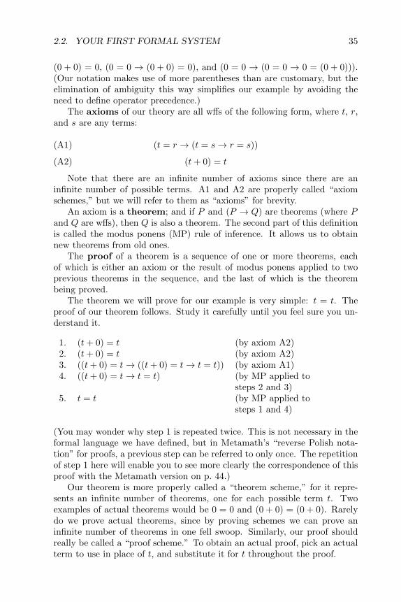
2.2. YOUR FIRST FORMAL SYSTEM 35
(0 + 0) = 0, (0 = 0 → (0 + 0) = 0), and (0 = 0 → (0 = 0 → 0 = (0 + 0))).(Our notation makes use of more parentheses than are customary, but theelimination of ambiguity this way simplifies our example by avoiding theneed to define operator precedence.)
The axioms of our theory are all wffs of the following form, where t, r,and s are any terms:
(t = r → (t = s→ r = s))(A1)
(t+ 0) = t(A2)
Note that there are an infinite number of axioms since there are aninfinite number of possible terms. A1 and A2 are properly called “axiomschemes,” but we will refer to them as “axioms” for brevity.
An axiom is a theorem; and if P and (P → Q) are theorems (where Pand Q are wffs), then Q is also a theorem. The second part of this definitionis called the modus ponens (MP) rule of inference. It allows us to obtainnew theorems from old ones.
The proof of a theorem is a sequence of one or more theorems, eachof which is either an axiom or the result of modus ponens applied to twoprevious theorems in the sequence, and the last of which is the theorembeing proved.
The theorem we will prove for our example is very simple: t = t. Theproof of our theorem follows. Study it carefully until you feel sure you un-derstand it.
1. (t+ 0) = t (by axiom A2)2. (t+ 0) = t (by axiom A2)3. ((t+ 0) = t→ ((t+ 0) = t→ t = t)) (by axiom A1)4. ((t+ 0) = t→ t = t) (by MP applied to
steps 2 and 3)5. t = t (by MP applied to
steps 1 and 4)
(You may wonder why step 1 is repeated twice. This is not necessary in theformal language we have defined, but in Metamath’s “reverse Polish nota-tion” for proofs, a previous step can be referred to only once. The repetitionof step 1 here will enable you to see more clearly the correspondence of thisproof with the Metamath version on p. 44.)
Our theorem is more properly called a “theorem scheme,” for it repre-sents an infinite number of theorems, one for each possible term t. Twoexamples of actual theorems would be 0 = 0 and (0 + 0) = (0 + 0). Rarelydo we prove actual theorems, since by proving schemes we can prove aninfinite number of theorems in one fell swoop. Similarly, our proof shouldreally be called a “proof scheme.” To obtain an actual proof, pick an actualterm to use in place of t, and substitute it for t throughout the proof.

36 CHAPTER 2. USING THE METAMATH PROGRAM
Let’s discuss what we have done here. The axioms of our theory, A1 andA2, are trivial and obvious. Everyone knows that adding zero to somethingdoesn’t change it, and also that if two things are equal to a third, then theyare equal to each other. In fact, stating the trivial and obvious is a goalto strive for in any axiomatic system. From trivial and obvious truths thateveryone agrees upon, we can prove results that are not so obvious yet haveabsolute faith in them. If we trust the axioms and the rules, we must, bydefinition, trust the consequences of those axioms and rules, if logic is tomean anything at all.
Our rule of inference, modus ponens, is also pretty obvious once youunderstand what it means. If we prove a fact P , and we also prove that Pimplies Q, then Q necessarily follows as a new fact. The rule provides uswith a means for obtaining new facts (i.e. theorems) from old ones.
The theorem that we have proved, t = t, is so fundamental that you maywonder why it isn’t one of the axioms. In some axiom systems of arithmetic,it is an axiom. The choice of axioms in a theory is to some extent arbitraryand even an art form, constrained only by the requirement that any twoequivalent axiom systems be able to derive each other as theorems. Wecould imagine that the inventor of our axiom system originally includedt = t as an axiom, then discovered that it could be derived as a theoremfrom the other axioms. Because of this, it was not necessary to keep it as anaxiom. By eliminating it, the final set of axioms became that much simpler.
Unless you have worked with formal proofs before, it probably wasn’tapparent to you that t = t could be derived from our two axioms until yousaw the proof. While you certainly believe that t = t is true, you might notbe able to convince an imaginary skeptic who believes only in our two axiomsuntil you produce the proof. Formal proofs such as this are hard to come upwith when you first start working with them, but after you get used to themthey can become interesting and fun. Once you understand the idea behindformal proofs you will have grasped the fundamental principle that underliesall of mathematics. As the mathematics becomes more sophisticated, itsproofs become more challenging, but ultimately they all can be broken downinto individual steps as simple as the ones in our proof above.
Mendelson’s book, from which our example was taken, contains a numberof detailed formal proofs such as these, and you may be interested in lookingit up. The book is intended for mathematicians, however, and most of itis rather advanced. Popular literature describing formal proofs include [51,p. 296] and [24, pp. 204–230].
2.2.2 Converting It to Metamath
Formal proofs such as the one in our example break down logical reasoninginto small, precise steps that leave little doubt that the results follow fromthe axioms. You might think that this would be the finest breakdown we canachieve in mathematics. However, there is more to the proof than meets the

2.2. YOUR FIRST FORMAL SYSTEM 37
eye. Although our axioms were rather simple, a lot of verbiage was neededbefore we could even state them: we needed to define “term,” “wff,” and soon. In addition, there are a number of implied rules that we haven’t evenmentioned. For example, how do we know that step 3 of our proof followsfrom axiom A1? There is some hidden reasoning involved in determiningthis. Axiom A1 has two occurrences of the letter t. One of the impliedrules states that whatever we substitute for t must be a legal term.5 Theexpression t+ 0 is pretty obviously a legal term whenever t is, but supposewe wanted to substitute a huge term with thousands of symbols? Certainlya lot of work would be involved in determining that it really is a term, but inordinary formal proofs all of this work would be considered a single “step.”
To express our axiom system in the Metamath language, we must de-scribe this auxiliary information in addition to the axioms themselves. Meta-math does not know what a “term” or a “wff” is. In Metamath, the specifi-cation of the ways in which we can combine symbols to obtain terms and wffsare like little axioms in themselves. These auxiliary axioms are expressed inthe same notation as the “real” axioms, and Metamath does not distinguishbetween the two. The distinction is made by you, i.e. by the way in whichyou interpret the notation you have chosen to express these two kinds ofaxioms.
The Metamath language breaks down mathematical proofs into tinypieces, much more so than in ordinary formal proofs. If a single step in-volves the substitution of a complex term for one of its variables, Metamathmust see this single step broken down into many small steps. This fine-grained breakdown is what gives Metamath generality and flexibility as itlets it not be limited to any particular mathematical notation.
Metamath’s proof notation is not, in itself, intended to be read by hu-mans but rather is in a compact format intended for a machine. The Meta-math program will convert this notation to a form you can understand, usingthe show proof command. You can tell the program what level of detailof the proof you want to look at. You may want to look at just the logicalinference steps that correspond to ordinary formal proof steps, or you maywant to see the fine-grained steps that prove that an expression is a term.
Here, without further ado, is our example converted to the Metamathlanguage:
$( Declare the constant symbols we will use $)
$c 0 + = -> ( ) term wff |- $.
$( Declare the metavariables we will use $)
$v t r s P Q $.
$( Specify properties of the metavariables $)
tt $f term t $.
5Some authors make this implied rule explicit by stating, “only expressions of theabove form are terms,” after defining “term.”

38 CHAPTER 2. USING THE METAMATH PROGRAM
tr $f term r $.
ts $f term s $.
wp $f wff P $.
wq $f wff Q $.
$( Define "term" and "wff" $)
tze $a term 0 $.
tpl $a term ( t + r ) $.
weq $a wff t = r $.
wim $a wff ( P -> Q ) $.
$( State the axioms $)
a1 $a |- ( t = r -> ( t = s -> r = s ) ) $.
a2 $a |- ( t + 0 ) = t $.
$( Define the modus ponens inference rule $)
${
min $e |- P $.
maj $e |- ( P -> Q ) $.
mp $a |- Q $.
$}
$( Prove a theorem $)
th1 $p |- t = t $=
$( Here is its proof: $)
tt tze tpl tt weq tt tt weq tt a2 tt tze tpl
tt weq tt tze tpl tt weq tt tt weq wim tt a2
tt tze tpl tt tt a1 mp mp
$.
A “database” is a set of one or more ascii source files. Here’s a briefdescription of this Metamath database (which consists of this single sourcefile), so that you can understand in general terms what is going on. Tounderstand the source file in detail, you should read Chapter 4.
The database is a sequence of “tokens,” which are normally separated byspaces or carriage returns. The only tokens that are built into the Metamathlanguage are those beginning with $. These tokens are called “keywords.”All other tokens are user-defined, and their names are arbitrary.
As you might have guessed, the Metamath token $( starts a commentand $) ends a comment.
The Metamath tokens $c, $v, $e, $f, $a, and $p specify “statements”that end with $. .
The Metamath tokens $c and $v each declare a list of user-defined tokens,called “math symbols,” that the database will reference later on. All of themath symbols they define you have seen earlier except the turnstile symbol|- (`), which is commonly used by logicians to mean “a proof exists for.”For us the turnstile is just a convenient symbol that distinguishes expressionsthat are axioms or theorems from expressions that are terms or wffs.
The $c statement declares “constants” and the $v statement declares

2.2. YOUR FIRST FORMAL SYSTEM 39
“variables” (or more precisely, metavariables). A variable may be substi-tuted with sequences of math symbols whereas a constant may not be sub-stituted with anything.
It may seem redundant to require both $c and $v statements (since anymath symbol not specified with a $c statement could be presumed to be avariable), but this provides for better error checking and also allows mathsymbols to be redeclared (Section 4.2.8).
The token $f specifies a statement called a “variable-type hypothesis”(also called a “floating hypothesis”) and $e specifies a “logical hypothesis”(also called an “essential hypothesis”). The token $a specifies an “axiomaticassertion,” and $p specifies a “provable assertion.” To the left of each oc-currence of these four tokens is a “label” that identifies the hypothesis orassertion for later reference. For example, the label of the first axiomaticassertion is tze. A $f statement must contain exactly two math symbols,a constant followed by a variable. The $e, $a, and $p statements eachstart with a constant followed by, in general, an arbitrary sequence of mathsymbols.
Associated with each assertion is a set of hypotheses that must be sat-isfied in order for the assertion to be used in a proof. These are called the“mandatory hypotheses” of the assertion. Among those hypotheses whose“scope” (described below) includes the assertion, $e hypotheses are alwaysmandatory and $f hypotheses are mandatory when they share their vari-able with the assertion or its $e hypotheses. The exact rules for determiningwhich hypotheses are mandatory are described in detail in Sections 4.2.7 and4.2.8. For example, the mandatory hypotheses of assertion tpl are tt andtr, whereas assertion tze has no mandatory hypotheses because it containsno variables and has no $e hypothesis. Metamath’s show statement com-mand, described in the next section, will show you a statement’s mandatoryhypotheses.
Sometimes we need to make a hypothesis relevant to only certain asser-tions. The set of statements to which a hypothesis is relevant is called its“scope.” The Metamath brackets, ${ and $}, define a “block” that delimitsthe scope of any hypothesis contained between them. The assertion mp hasmandatory hypotheses wp, wq, min, and maj. The only mandatory hypoth-esis of th1, on the other hand, is tt, since th1 occurs outside of the blockcontaining min and maj.
Note that ${ and $} do not affect the scope of assertions ($a and $p).Assertions are always available to be referenced by any later proof in thesource file.
Each provable assertion ($p statement) has two parts. The first partis the assertion itself, which is a sequence of math symbol tokens placedbetween the $p token and a $= token. The second part is a “proof,” which isa list of label tokens placed between the $= token and the $. token that ends

40 CHAPTER 2. USING THE METAMATH PROGRAM
the statement.6 The proof acts as a series of instructions to the Metamathprogram, telling it how to build up the sequence of math symbols containedin assertion part of the $p statement, making use of the hypotheses of the $pstatement and previous assertions. The construction takes place accordingto precise rules. If the list of labels in the proof causes these rules to beviolated, or if the final sequence that results does not match the assertion,the Metamath program will notify you with an error message.
If you are familiar with reverse Polish notation (RPN), which is some-times used on pocket calculators, here in a nutshell is how a proof works.Each hypothesis label in the proof is pushed onto the RPN stack as it isencountered. Each assertion label pops off the stack as many entries as thereferenced assertion has mandatory hypotheses. Variable substitutions arecomputed which, when made to the referenced assertion’s mandatory hy-potheses, cause these hypotheses to match the stack entries. These samesubstitutions are then made to the variables in the referenced assertion it-self, which is then pushed onto the stack. At the end of the proof, thereshould be one stack entry, namely the assertion being proved. This processis explained in detail in Section 4.3.
Metamath’s proof notation is not very readable for humans, but it allowsthe proof to be stored compactly in a file. The Metamath program has proofdisplay features that let you see what’s going on in a more readable way, asyou will see in the next section.
The rules used in verifying a proof are not based on any built-in syntax ofthe symbol sequence in an assertion nor on any built-in meanings attachedto specific symbol names. They are based strictly on symbol matching: con-stants must match themselves, and variables may be replaced with anythingthat allows a match to occur. For example, instead of term, 0, and |- wecould have just as well used yellow, zero, and provable, as long as wedid so consistently throughout the database. Also, we could have used is
provable (two tokens) instead of |- (one token) throughout the database.In each of these cases, the proof would be exactly the same. The inde-pendence of proofs and notation means that you have a lot of flexibility tochange the notation you use without having to change any proofs.
2.3 A Trial Run
Now you are ready to try out the Metamath program.On all computer systems, Metamath has a standard “command line in-
terface” (CLI) that allows you to interact with it. You supply commandsto the CLI by typing them on the keyboard and pressing your keyboard’s
6If you’ve looked at the set.mm database, you may have noticed another notation usedfor proofs. The other notation is called “compressed.” It reduces the amount of spaceneeded to store a proof in the database and is described in Appendix B. In the exampleabove, we use “normal” notation.

2.3. A TRIAL RUN 41
return key after each line you enter. The CLI is designed to be easy to useand has built-in help features.
The first thing you should do is to use a text editor to create a file calleddemo0.mm and type into it the Metamath source shown on p. 37. Actually,this file is included with your Metamath software package, so check thatfirst. If you type it in, make sure that you save it in the form of “plain asciitext with line breaks.” Most word processors will have this feature.
Next you must run the Metamath program. Depending on your com-puter system and how Metamath is installed, this could range from clickingthe mouse on the Metamath icon to typing run metamath to typing simplymetamath. (Metamath’s help invoke command describes alternate ways ofinvoking the Metamath program.)
When you first enter Metamath, it will be at the CLI, waiting for yourinput. You will see the following on your screen:
Metamath - Version 0.07.30 8-Feb-2007
Type HELP for help, EXIT to exit.
MM>
The MM> prompt means that Metamath is waiting for a command. (Thehelp message line suggests that commands should be typed in upper case,but actually command keywords are not case sensitive. We will use lowercase in our examples.)
The first thing that you need to do is to read in your database:7
MM> read demo0.mm
Remember to press the return key after entering this command. If you omitthe file name, Metamath will prompt you for one. The syntax for specifyinga Macintosh file name path is given in a footnote on p. 123.
If there are any syntax errors in the database, Metamath will let youknow when it reads in the file. The one thing that Metamath does notcheck when reading in a database is that all proofs are correct, because thiswould slow it down too much. It is a good idea to periodically verify theproofs in a database you are making changes to. To do this, use the followingcommand (and do it for your demo0.mm file now). Note that the * is a “wildcard” meaning all proofs in the file.
MM> verify proof *
Metamath will report any proofs that are incorrect.It is often useful to save the information that the Metamath program
displays on the screen. You can save everything that happens on the screenby opening a log file. You may want to do this before you read in a databaseso that you can examine any errors later on. To open a log file, type
7If a directory path is needed on Unix, you should enclose the path/file name in quotesto prevent Metamath from thinking that the / in the path name is a command qualifier,e.g., read "db/set.mm". Quotes are optional when there is no ambiguity.

42 CHAPTER 2. USING THE METAMATH PROGRAM
MM> open log abc.log
This will open a file called abc.log, and everything that appears on thescreen from this point on will be stored in this file. The name of the log fileis arbitrary. To close the log file, type
MM> close log
Several commands let you examine what’s inside of your database. Sec-tion 3.8 has an overview of some useful ones. The show labels commandlets you see what statement labels exist. A * matches any combination ofcharacters, and t* refers to all labels starting with the letter t. The /all isa “command qualifier” that tells Metamath to include labels of hypotheses.(To see the syntax explained, type help show labels.) Type
MM> show labels t* /all
Metamath will respond with
The statement number, label, and type are shown.
3 tt $f 4 tr $f 5 ts $f 8 tze $a
9 tpl $a 19 th1 $p
You can use the show statement command to get information abouta particular statement. For example, you can get information about thestatement with label mp by typing
MM> show statement mp /full
Metamath will respond with
Statement 17 is located on line 43 of the file
"demo0.mm".
"Define the modus ponens inference rule"
17 mp $a |- Q $.
Its mandatory hypotheses in RPN order are:
wp $f wff P $.
wq $f wff Q $.
min $e |- P $.
maj $e |- ( P -> Q ) $.
The statement and its hypotheses require the
variables: Q P
The variables it contains are: Q P
The mandatory hypotheses and their order are useful to know when you aretrying to understand or debug a proof.
Now you are ready to look at what’s really inside of our proof. First, hereis how to look at every step in the proof—not just the ones correspondingto an ordinary formal proof, but also the ones that build up the formulasthat appear in each ordinary formal proof step.

2.3. A TRIAL RUN 43
MM> show proof th1 /lemmon /all
This will display the proof on the screen in the following format:
1 tt $f term t
2 tze $a term 0
3 1,2 tpl $a term ( t + 0 )
4 tt $f term t
5 3,4 weq $a wff ( t + 0 ) = t
6 tt $f term t
7 tt $f term t
8 6,7 weq $a wff t = t
9 tt $f term t
10 9 a2 $a |- ( t + 0 ) = t
11 tt $f term t
12 tze $a term 0
13 11,12 tpl $a term ( t + 0 )
14 tt $f term t
15 13,14 weq $a wff ( t + 0 ) = t
16 tt $f term t
17 tze $a term 0
18 16,17 tpl $a term ( t + 0 )
19 tt $f term t
20 18,19 weq $a wff ( t + 0 ) = t
21 tt $f term t
22 tt $f term t
23 21,22 weq $a wff t = t
24 20,23 wim $a wff ( ( t + 0 ) = t -> t = t )
25 tt $f term t
26 25 a2 $a |- ( t + 0 ) = t
27 tt $f term t
28 tze $a term 0
29 27,28 tpl $a term ( t + 0 )
30 tt $f term t
31 tt $f term t
32 29,30,31 a1 $a |- ( ( t + 0 ) = t -> ( ( t + 0 )
= t -> t = t ) )
33 15,24,26,32 mp $a |- ( ( t + 0 ) = t -> t = t )
34 5,8,10,33 mp $a |- t = t
The /lemmon command qualifier specifies what is known as a Lemmon-style display. Omitting the /lemmon qualifier results in a tree-style proof (seep. 117 for an example) that is somewhat less explicit but easier to followonce you get used to it.
The first number on each line is the step number of the proof. Anynumbers that follow are step numbers assigned to the hypotheses of the

44 CHAPTER 2. USING THE METAMATH PROGRAM
statement referenced by that step. Next is the label of the statement refer-enced by the step. The statement type of the statement referenced comesnext, followed by the math symbol string constructed by the proof up tothat step.
The last step, 34, contains the statement that is being proved.Looking at a small piece of the proof, notice that steps 3 and 4 have
established that ( t + 0 ) and t are term s, and step 5 makes use of steps3 and 4 to establish that ( t + 0 ) = t is a wff. Let us let Metamathitself tell us in detail what is happening in step 5. Note that the “targethypothesis” refers to where step 5 is eventually used, i.e., in step 34.
MM> show proof th1 /detailed_step 5
Proof step 5: wp=weq $a wff ( t + 0 ) = t
This step assigns source "weq" ($a) to target "wp"
($f). The source assertion requires the hypotheses
"tt" ($f, step 3) and "tr" ($f, step 4). The parent
assertion of the target hypothesis is "mp" ($a,
step 34).
The source assertion before substitution was:
weq $a wff t = r
The following substitutions were made to the source
assertion:
Variable Substituted with
t ( t + 0 )
r t
The target hypothesis before substitution was:
wp $f wff P
The following substitution was made to the target
hypothesis:
Variable Substituted with
P ( t + 0 ) = t
The full proof just shown is useful to understand what is going on in de-tail. However, most of the time you will just be interested in the “essential”or logical steps of a proof, i.e. those steps that correspond to an ordinaryformal proof. If you type
MM> show proof th1 /essential /lemmon /renumber
you will see
1 a2 $a |- ( t + 0 ) = t
2 a2 $a |- ( t + 0 ) = t
3 a1 $a |- ( ( t + 0 ) = t -> ( ( t + 0 )
= t -> t = t ) )
4 2,3 mp $a |- ( ( t + 0 ) = t -> t = t )
5 1,4 mp $a |- t = t

2.3. A TRIAL RUN 45
Compare this to the formal proof on p. 35 and notice the resemblance. The/essential qualifier in the show proof command tells Metamath to dis-card all $f hypotheses and everything branching off of them in the proof treewhen the proof is displayed; this makes the proof look more like an ordinarymathematical proof, which does not normally incorporate the explicit con-struction of expressions. The /renumber qualifier means to renumber thesteps to correspond only to what is displayed.
To exit Metamath, type
MM> exit
2.3.1 Some Hints for Using the Command Line Inter-face
We will conclude this quick introduction to Metamath with some helpfulhints on how to navigate your way through the commands.
When you type commands into Metamath’s CLI, you only have to typeas many characters of a command keyword as are needed to make it un-ambiguous. If you type too few characters, Metamath will tell you whatthe choices are. In the case of the read command, only the r is needed tospecify it unambiguously, so you could have typed
MM> r demo0.mm
instead of
MM> read demo0.mm
In our description, we always show the full command words. When using theMetamath CLI commands in a command file (to be read with the submit
command), it is good practice to use the unabbreviated command to ensureyour instructions will not become ambiguous if more commands are addedto the Metamath program in the future.
The command keywords are not case sensitive; you may type either reador ReAd. File names may or may not be case sensitive, depending on yourcomputer’s operating system. Metamath label and math symbol tokens arecase-sensitive.
The help command will provide you with a list of topics you can gethelp on. You can then type help topic to get help on that topic.
If you are uncertain of a command’s spelling, just type as many char-acters as you remember of the command. If you have not typed enoughcharacters to specify it unambiguously, Metamath will tell you what choicesyou have.
MM> show s
^
?Ambiguous keyword - please specify SETTINGS,
STATEMENT, or SOURCE.

46 CHAPTER 2. USING THE METAMATH PROGRAM
If you don’t what know argument to use as part of a command, type a? at the argument position. Metamath will tell you what it expected there.
MM> show ?
^
?Expected SETTINGS, LABELS, STATEMENT, SOURCE, PROOF,
MEMORY, TRACE_BACK, or USAGE.
Finally, you may type just the first word or words of a command followedby return. Metamath will prompt you for the remaining part of the com-mand, showing you the choices at each step. For example, instead of typingshow statement th1 /full you could interact in the following manner:
MM> show
SETTINGS, LABELS, STATEMENT, SOURCE, PROOF,
MEMORY, TRACE_BACK, or USAGE <SETTINGS>? st
What is the statement label <th1>?
/ or nothing <nothing>? /
TEX, COMMENT_ONLY, or FULL <TEX>? f
/ or nothing <nothing>?
19 th1 $p |- t = t $= ... $.
After each ? in this mode, you must give Metamath the information itrequests. Sometimes Metamath gives you a list of choices with the defaultchoice indicated by brackets < > . Pressing return after the ? will select thedefault choice. Answering anything else will override the default. Note thatthe / in command qualifiers is considered a separate token by the parser,and this is why it is asked for separately.
2.4 Your First Proof
Proofs are developed with the aid of the Proof Assistant. We will now showyou how the proof of theorem th1 was built. So that you can repeat thesesteps, we will first have the Proof Assistant erase the proof in Metamath’ssource buffer, then reconstruct it. (The source buffer is the place in memorywhere Metamath stores the information in the database when it is read
in. New or modified proofs are kept in the source buffer until a write
source command is issued.) In practice, you would place a ? between $=
and $. in the database to indicate to Metamath that the proof is unknown,and that would be your starting point. Whenever verify proof commandencounters a proof with a ? in place of a proof step, the statement is identifiedas not proved.
Before you start, you should write down on a piece of paper the completeformal proof as it would appear with the /essential qualifier in a show
proof command; see the display of show proof th1 /essential /lemmon

2.4. YOUR FIRST PROOF 47
/renumber above as an example. After you get used to using the ProofAssistant you may get to a point where you can “see” the proof in yourmind and let the Proof Assistant guide you in filling in the details, at leastfor simpler proofs, but until you gain that experience it is important to writedown all the details in advance. Otherwise you may waste a lot of time asyou let it take you down a wrong path.
A proof is developed with the Proof Assistant by working backwards,starting with the theorem to be proved, and assigning each unknown stepwith a theorem or hypothesis until no more unknown steps remain. TheProof Assistant will not let you make an assignment unless it can be “uni-fied” with the unknown step. This means that a substitution of variablesexists that will make the assignment match the unknown step. On the otherhand, in the middle of a proof, when working backwards, often more thanone unification (set of substitutions) is possible, since there is not enoughinformation available at that point to uniquely establish it. In this case youcan tell Metamath which unification to choose, or you can continue to assignunknown steps until enough information is available to make the unificationunique.
We will assume you have entered Metamath and read in the database asdescribed above. The following dialog shows how the proof was developed.For more details on what some of the commands do, refer to Section 5.6.
MM> prove th1
Entering the Proof Assistant. Type HELP for help, EXIT
to exit. You will be working on the proof of statement th1:
$p |- t = t
Note: The proof you are starting with is already complete.
MM-PA>
The MM-PA> prompt means we are inside of the Proof Assistant. Most ofthe regular Metamath commands (show statement, etc.) are still availableif you need them.
MM-PA> delete all
The entire proof was deleted.
We have deleted the whole proof so we can start from scratch.
MM-PA> show new_proof/lemmon/all
1 ? $? |- t = t
The show new_proof command is like show proof except that we don’tspecify a statement; instead, the proof we’re working on is displayed.
MM-PA> assign 1 mp
To undo the assignment, DELETE STEP 5 and INITIALIZE, UNIFY
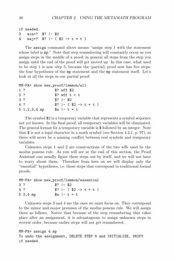
48 CHAPTER 2. USING THE METAMATH PROGRAM
if needed.
3 min=? $? |- $2
4 maj=? $? |- ( $2 -> t = t )
The assign command above means “assign step 1 with the statementwhose label is mp.” Note that step renumbering will constantly occur as youassign steps in the middle of a proof; in general all steps from the step youassign until the end of the proof will get moved up. In this case, what usedto be step 1 is now step 5, because the (partial) proof now has five steps:the four hypotheses of the mp statement and the mp statement itself. Let’slook at all the steps in our partial proof:
MM-PA> show new_proof/lemmon/all
1 ? $? wff $2
2 ? $? wff t = t
3 ? $? |- $2
4 ? $? |- ( $2 -> t = t )
5 1,2,3,4 mp $a |- t = t
The symbol $2 is a temporary variable that represents a symbol sequencenot yet known. In the final proof, all temporary variables will be eliminated.The general format for a temporary variable is $ followed by an integer. Notethat $ is not a legal character in a math symbol (see Section 4.2.1, p. 97), sothere will never be a naming conflict between real symbols and temporaryvariables.
Unknown steps 1 and 2 are constructions of the two wffs used by themodus ponens rule. As you will see at the end of this section, the ProofAssistant can usually figure these steps out by itself, and we will not haveto worry about them. Therefore from here on we will display only the“essential” hypotheses, i.e. those steps that correspond to traditional formalproofs.
MM-PA> show new_proof/lemmon/essential
3 ? $? |- $2
4 ? $? |- ( $2 -> t = t )
5 3,4 mp $a |- t = t
Unknown steps 3 and 4 are the ones we must focus on. They correspondto the minor and major premises of the modus ponens rule. We will assignthem as follows. Notice that because of the step renumbering that takesplace after an assignment, it is advantageous to assign unknown steps inreverse order, because earlier steps will not get renumbered.
MM-PA> assign 4 mp
To undo the assignment, DELETE STEP 8 and INITIALIZE, UNIFY
if needed.

2.4. YOUR FIRST PROOF 49
3 min=? $? |- $2
6 min=? $? |- $4
7 maj=? $? |- ( $4 -> ( $2 -> t = t ) )
We are now going to describe an obscure feature that you will probablynever use but should be aware of. The Metamath language allows emptysymbol sequences to be substituted for variables, but in most formal systemsthis feature is never used. One of the few examples where is it used is theMIU-system described in Appendix D. But such systems are rare, and bydefault this feature is turned off in the Proof Assistant. (It is always allowedfor verify proof.) Let us turn it on and see what happens.
MM-PA> set empty_substitution on
Substitutions with empty symbol sequences is now allowed.
With this feature enabled, more unifications will be ambiguous in themiddle of a proof, because substitution of variables with empty symbol se-quences will become an additional possibility. Let’s see what happens whenwe make our next assignment.
MM-PA> assign 3 a2
There are 2 possible unifications. Please select the correct
one or Q if you want to UNIFY later.
Unify: |- $6
with: |- ( $9 + 0 ) = $9
Unification #1 of 2 (weight = 7):
Replace "$6" with "( + 0 ) ="
Replace "$9" with ""
Accept (A), reject (R), or quit (Q) <A>? r
The first choice presented is the wrong one. If we had selected it, tempo-rary variable $6 would have been assigned a truncated wff, and temporaryvariable $9 would have been assigned an empty sequence (which is not al-lowed in our system). With this choice, eventually we would reach a pointwhere we would get stuck because we would end up with steps impossibleto prove. (You may want to try it.) We typed r to reject the choice.
Unification #2 of 2 (weight = 21):
Replace "$6" with "( $9 + 0 ) = $9"
Accept (A), reject (R), or quit (Q) <A>? q
To undo the assignment, DELETE STEP 4 and INITIALIZE, UNIFY
if needed.
7 min=? $? |- $8
8 maj=? $? |- ( $8 -> ( $6 -> t = t ) )
The second choice is correct, and normally we would type a to acceptit. But instead we typed q to show what will happen: it will leave the stepwith an unknown unification, which can be seen as follows:

50 CHAPTER 2. USING THE METAMATH PROGRAM
MM-PA> show new_proof/not_unified
4 min $a |- $6
=a2 = |- ( $9 + 0 ) = $9
Later we can unify this with the unify all/interactive command.The important point to remember is that occasionally you will be pre-
sented with several unification choices while entering a proof, when theprogram determines that there is not enough information yet to make anunambiguous choice automatically (and this can happen even with set
empty_substitution turned off). Usually it is obvious by inspection whichchoice is correct, since incorrect ones will tend to be meaningless fragmentsof wffs. In addition, the correct choice will usually be the first one presented,unlike our example above.
Enough of this digression. Let us go back the the default setting.
MM-PA> set empty_substitution off
The ability to substitute empty expressions for variables
has been turned off. Note that this may make the Proof
Assistant too restrictive in some cases.
If we delete the proof, start over, and get to the point where we digressedabove, there will no longer be an ambiguous unification.
MM-PA> assign 3 a2
To undo the assignment, DELETE STEP 4 and INITIALIZE, UNIFY
if needed.
7 min=? $? |- $4
8 maj=? $? |- ( $4 -> ( ( $5 + 0 ) = $5 -> t = t ) )
Let us look at our proof so far, and continue.
MM-PA> show new_proof/lemmon
4 a2 $a |- ( $5 + 0 ) = $5
7 ? $? |- $4
8 ? $? |- ( $4 -> ( ( $5 + 0 ) = $5 -> t = t ) )
9 7,8 mp $a |- ( ( $5 + 0 ) = $5 -> t = t )
10 4,9 mp $a |- t = t
MM-PA> assign 8 a1
To undo the assignment, DELETE STEP 11 and INITIALIZE, UNIFY
if needed.
7 min=? $? |- ( t + 0 ) = t
MM-PA> assign 7 a2
To undo the assignment, DELETE STEP 8 and INITIALIZE, UNIFY
if needed.
MM-PA> show new_proof/lemmon
4 a2 $a |- ( t + 0 ) = t

2.4. YOUR FIRST PROOF 51
8 a2 $a |- ( t + 0 ) = t
12 a1 $a |- ( ( t + 0 ) = t -> ( ( t + 0 ) = t ->
t = t ) )
13 8,12 mp $a |- ( ( t + 0 ) = t -> t = t )
14 4,13 mp $a |- t = t
Now all temporary variables and unknown steps have been eliminatedfrom the “essential” part of the proof. When this is achieved, the ProofAssistant can usually figure out the rest of the proof automatically. (Notethat the improve command can occasionally be useful for filling in essentialsteps as well, but it only tries to make use of statements that introduce nonew variables in their hypotheses, which is not the case for mp. Also it willnot try to improve steps containing temporary variables.) Let’s look at thecomplete proof, then run the improve command, then look at it again.
MM-PA> show new_proof/lemmon/all
1 ? $? wff ( t + 0 ) = t
2 ? $? wff t = t
3 ? $? term t
4 3 a2 $a |- ( t + 0 ) = t
5 ? $? wff ( t + 0 ) = t
6 ? $? wff ( ( t + 0 ) = t -> t = t )
7 ? $? term t
8 7 a2 $a |- ( t + 0 ) = t
9 ? $? term ( t + 0 )
10 ? $? term t
11 ? $? term t
12 9,10,11 a1 $a |- ( ( t + 0 ) = t -> ( ( t + 0 ) = t ->
t = t ) )
13 5,6,8,12 mp $a |- ( ( t + 0 ) = t -> t = t )
14 1,2,4,13 mp $a |- t = t
MM-PA> improve all
A proof of length 1 was found for step 11.
A proof of length 1 was found for step 10.
A proof of length 3 was found for step 9.
A proof of length 1 was found for step 7.
A proof of length 9 was found for step 6.
A proof of length 5 was found for step 5.
A proof of length 1 was found for step 3.
A proof of length 3 was found for step 2.
A proof of length 5 was found for step 1.
Steps 1 and above have been renumbered.
CONGRATULATIONS! The proof is complete. Use SAVE
NEW_PROOF to save it. Note: The Proof Assistant does

52 CHAPTER 2. USING THE METAMATH PROGRAM
not detect $d violations. After saving the proof, you
should verify it with VERIFY PROOF.
The save new_proof command will save the proof in the database. Herewe will just display it in a form that can be clipped out of a log file andinserted manually into the database source file with a text editor.
MM-PA> show new_proof/normal
---------Clip out the proof below this line:
tt tze tpl tt weq tt tt weq tt a2 tt tze tpl tt weq
tt tze tpl tt weq tt tt weq wim tt a2 tt tze tpl tt
tt a1 mp mp $.
---------The proof of ’th1’ to clip out ends above this line.
There is another proof format called “compressed” that you will seein databases. It is not important to understand how it is encoded butonly to recognize it when you see it. Its only purpose is to reduce storagerequirements for large proofs. A compressed proof can always be convertedto a normal one and vice-versa, and the Metamath show proof commandswork equally well with compressed proofs. The compressed proof format isdescribed in Appendix B.
MM-PA> show new_proof/compressed
---------Clip out the proof below this line:
( tze tpl weq a2 wim a1 mp ) ABCZADZAADZAEZJJKFLIA
AGHH $.
---------The proof of ’th1’ to clip out ends above this line.
Now we will exit the Proof Assistant. Since we made changes to theproof, it will warn us that we have not saved it. In this case, we don’t care.
MM-PA> exit
Warning: You have not saved changes to the proof.
Do you want to EXIT anyway (Y, N) <N>? y
Exiting the Proof Assistant.
Type EXIT again to exit Metamath.
The Proof Assistant has several other commands that can help you whilecreating proofs. See Section 5.6 for a list of them.
A command that is often useful is minimize_with */brief, which triesto shorten the proof. It can make the process more efficient by letting youwrite a somewhat “sloppy” proof then clean up some of the fine details of op-timization for you (although it can’t perform miracles such as restructuringthe overall proof).

2.5. A NOTE ABOUT EDITING A DATABASE FILE 53
2.5 A Note About Editing a Database File
Once your source file contains proofs, there are some restrictions on howyou can edit it so that the proofs remain valid. Pay particular attention tothese rules, since otherwise you can lose a lot of work. It is a good idea toperiodically verify all proofs with verify proof * to ensure their integrity.
If your file contains only normal (as opposed to compressed) proofs, themain rule is that you may not change the order of the mandatory hypothesesof any statement referenced in a later proof. For example, if you swapthe order of the major and minor premise in the modus ponens rule, allproofs making use of that rule will become incorrect. The show statement
command will show you the mandatory hypotheses of a statement and theirorder.
If a statement has a compressed proof, you also must not change theorder of its mandatory hypotheses. The compressed proof format makesuse of this information as part of the compression technique. Note thatswapping the names of two variables in a theorem will change the order ofits mandatory hypotheses.
The safest way to edit a statement, say mytheorem, is to duplicate itthen rename the original to mytheoremOLD throughout the database. Oncethe edited version is re-proved, all statements referencing mytheoremOLD
can be updated in the Proof Assistant using minimize_with mytheorem
/allow_growth.

54 CHAPTER 2. USING THE METAMATH PROGRAM

Chapter 3
Abstract MathematicsRevealed
3.1 Logic and Set Theory
Set theory can be viewed as a form of exact theology.
Rudy Rucker1
Despite its seeming complexity, all of standard mathematics, no matterhow deep or abstract, can amazingly enough be derived from a relativelysmall set of axioms or first principles. The development of these axioms isamong the most impressive and important accomplishments of mathematicsin the 20th century. Ultimately, these axioms can be broken down into a setof rules for manipulating symbols that any technically oriented person canfollow.
We will not spend much time trying to convey a deep, higher-level under-standing of the meaning of the axioms. This kind of understanding requiressome mathematical sophistication as well as an understanding of the phi-losophy underlying the foundations of mathematics and typically developsover time as you work with mathematics. Our goal, instead, is to give youthe immediate ability to follow how theorems are derived from the axiomsand from other theorems. This will be similar to learning the syntax of acomputer language, which lets you follow the details in a program but doesnot necessarily give you the ability to write non-trivial programs on yourown, an ability that comes with practice. For now don’t be alarmed byabstract-sounding names of the axioms; just focus on the rules for manip-ulating the symbols, which follow the simple conventions of the Metamathlanguage.
1[3], p. 31
55

56 CHAPTER 3. ABSTRACT MATHEMATICS REVEALED
The axioms that underlie all of standard mathematics consist of axiomsof logic and axioms of set theory. The axioms of logic are divided into twosubcategories, propositional calculus (sometimes called sentential logic) andpredicate calculus (sometimes called first-order logic or quantifier theory).Propositional calculus is a prerequisite for predicate calculus, and predicatecalculus is a prerequisite for set theory. The version of set theory mostcommonly used is Zermelo-Fraenkel set theory.
Here in a nutshell is what the axioms are all about in an informal way.The connection between this description and symbols we will show you won’tbe immediately apparent and in principle needn’t ever be. Our descriptionjust tries to summarize what mathematicians think about when they workwith the axioms.
Logic is more or less the translation of what we would consider commonsense into a rigorous set of axioms. Suppose ϕ, ψ, and χ (the Greek lettersphi, psi, and chi) represent statements that are either true or false, and x isa variable ranging over some group of mathematical objects (sets, integers,real numbers, etc.). In mathematics, a “statement” really means a formula,and ψ could be for example “x = 2.” Logic makes assertions such as “if ϕimplies ψ and ψ implies χ, then ϕ implies χ” (propositional calculus) and“if ϕ is true for all x, then ϕ is true for some x” (predicate calculus).
Set theory has to do with the manipulation of objects and collections ofobjects, specifically the abstract, imaginary objects that mathematics dealswith, such as numbers. Everything that is claimed to exist in mathematicsis considered to be a set. A set called the empty set contains nothing. Werepresent the empty set by ∅. Many sets can be built up from the emptyset. There is a set represented by {∅} that contains the empty set, anotherset represented by {∅, {∅}} that contains this set as well as the empty set,another set represented by {{∅}} that contains just the set that containsthe empty set, and so on ad infinitum. All mathematical objects, no matterhow complex, are defined as being identical to certain sets: the integer 0is defined as the empty set, the integer 1 is defined as {∅}, the integer 2is defined as {∅, {∅}}. (How these definitions were chosen doesn’t matternow, but the idea behind it is that these sets have the properties we expectof integers once suitable operations are defined.) Mathematical operations,such as addition, are defined in terms of operations on sets—their union,intersection, and so on—operations you may have used in elementary schoolwhen you worked with groups of apples and oranges.
With a leap of faith, the axioms also postulate the existence of infinitesets, such as the set of all non-negative integers (0, 1, 2, . . ., also called “natu-ral numbers”). This set can’t be represented with the brace notation we justshowed you, but requires a more complicated notation called “class abstrac-tion.” For example, the infinite set {x|“x is a natural number”} means the“set of all objects x such that x is a natural number” i.e. the set of naturalnumbers; here, “x is a natural number” is a rather complicated formula when
3.1. LOGIC AND SET THEORY 57
broken down into the primitive symbols.2 Actually, the primitive symbolsdon’t even include the brace notation. The brace notation is a high-leveldefinition, which you can find in Section 3.4.
Interestingly, the arithmetic of integers and rationals can be developedwithout appealing to the existence of an infinite set, whereas the arithmeticof real numbers requires it.
Each variable in the axioms of set theory represents an arbitrary set, andthe axioms specify the legal kinds of things you can do with these variablesat a very primitive level.
Now, you may think that numbers and arithmetic are a lot more intu-itive and fundamental than sets and therefore should be the foundation ofmathematics. What is really the case is that you’ve dealt with numbers allyour life and are comfortable with a few rules for manipulating them suchas addition and multiplication. Those rules only cover a small portion ofwhat can be done with numbers and only a very tiny fraction of the rest ofmathematics. If you look at any elementary book on number theory, you willquickly become lost if these are the only rules that you know. Even thoughsuch books may present a list of “axioms” for arithmetic, the ability to usethe axioms and to understand proofs of theorems (facts) about numbersrequires an implicit mathematical talent that frustrates many people fromstudying abstract mathematics. The kind of mathematics that most peopleknow limits them to the practical, everyday usage of blindly manipulatingnumbers and formulas, without any understanding of why those rules arecorrect nor any ability to go any further. For example, do you know whymultiplying two negative numbers yields a positive number? Starting withset theory, you will also start off blindly manipulating symbols accordingto the rules we give you, but with the advantage that these rules will allowyou, in principle, to access all of mathematics, not just a tiny part of it.
Of course, concrete examples are often helpful in the learning process.For example, you can verify that that 2 · 3 = 3 · 2 by actually groupingobjects and can easily “see” how it generalizes to x · y = y · x, even thoughyou might not be able to rigorously prove it. Similarly, in set theory it canbe helpful to understand how the axioms of set theory apply to (and arecorrect for) small finite collections of objects. You should be aware that in
2The statement “x is a natural number” is formally expressed as “x ∈ ω,” where ∈(stylized epsilon) means “is in” or “is an element of” and ω (omega) means “the setof natural numbers.” When “x ∈ ω” is completely expanded in terms of the primitivesymbols of set theory, the result is ¬ ( ¬ ( ∀ z ( ¬ ∀ w ( z ∈ w → ¬ w ∈ x ) → z ∈ x )→ ( ∀ z ( ¬ ( ∀ w ( w ∈ z → w ∈ x ) → ∀ w ¬ w ∈ z ) → ¬ ∀ w ( w ∈ z → ¬ ∀ v ( v ∈z → ¬ v ∈ w ) ) ) → ¬ ∀ z ∀ w ( ¬ ( z ∈ x → ¬ w ∈ x ) → ( ¬ z ∈ w → ( ¬ z = w →w ∈ z ) ) ) ) ) → ¬ ∀ y ( ¬ ( ¬ ( ∀ z ( ¬ ∀ w ( z ∈ w → ¬ w ∈ y ) → z ∈ y ) → ( ∀ z (¬ ( ∀ w ( w ∈ z → w ∈ y ) → ∀ w ¬ w ∈ z ) → ¬ ∀ w ( w ∈ z → ¬ ∀ v ( v ∈ z → ¬ v∈ w ) ) ) → ¬ ∀ z ∀ w ( ¬ ( z ∈ y → ¬ w ∈ y ) → ( ¬ z ∈ w → ( ¬ z = w → w ∈ z ) )) ) → ( ∀ z ¬ z ∈ y → ¬ ∀ w ( ¬ ( w ∈ y → ¬ ∀ z ( w ∈ z → ¬ z ∈ y ) ) → ¬ ( ¬ ∀ z( w ∈ z → ¬ z ∈ y ) → w ∈ y ) ) ) ) → x ∈ y ) ) ). Section 3.4 shows the hierarchy ofdefinitions that leads up to this expression.

58 CHAPTER 3. ABSTRACT MATHEMATICS REVEALED
set theory intuition can be misleading for infinite collections, and rigorousproofs become more important. For example, while x · y = y · x is correctfor finite ordinals (which are the natural numbers), it is not usually true forinfinite ordinals.
3.2 The Axioms for All of Mathematics
In this section, we will show you the axioms for all of standard mathematics(i.e. logic and set theory) as they are traditionally presented. The tradi-tional presentation is useful for someone with the mathematical experienceneeded to correctly manipulate high-level abstract concepts. For someonewithout this talent, knowing how to actually make use of these axioms canbe difficult. The purpose of this section is to allow you to see how the ver-sion of the axioms used in the standard Metamath database set.mm relatesto the typical version in textbooks, and also to give you an informal feel forthem.
3.2.1 Propositional Calculus
Propositional calculus concerns itself with statements that can be inter-preted as either true or false. Some examples of statements (outside ofmathematics) that are either true or false are “It is raining today” and “TheUnited States has a female president.” In mathematics, as we mentioned,statements are really formulas.
In propositional calculus, we don’t care what the statements are. We alsotreat a logical combination of statements, such as “It is raining today and theUnited States has a female president,” no differently from a single statement.Statements and their combinations are called well-formed formulas (wffs).We define wffs only in terms of other wffs and don’t define what a “starting”wff is. As is common practice in the literature, we use Greek letters torepresent wffs.
Specifically, suppose ϕ and ψ are wffs. Then the combinations ϕ → ψ(“ϕ implies ψ,” also read “if ϕ then ψ”) and ¬ϕ (“not ϕ”) are also wffs.
The three axioms of propositional calculus are all wffs of the followingform:3
ϕ→ (ψ → ϕ)(ϕ→ (ψ → χ))→ ((ϕ→ ψ)→ (ϕ→ χ))
(¬ϕ→ ¬ψ)→ (ψ → ϕ)
There are an infinite number of axioms, one for each possible wff ofthe above form. (For this reason, axioms such as the above are often called
3A remarkable result of C. A. Meredith squeezes these three axioms into the singleaxiom ((((ϕ → ψ) → (¬χ → ¬θ)) → χ) → τ) → ((τ → ϕ) → (θ → ϕ)) [37], which isbelieved to be the shortest possible.
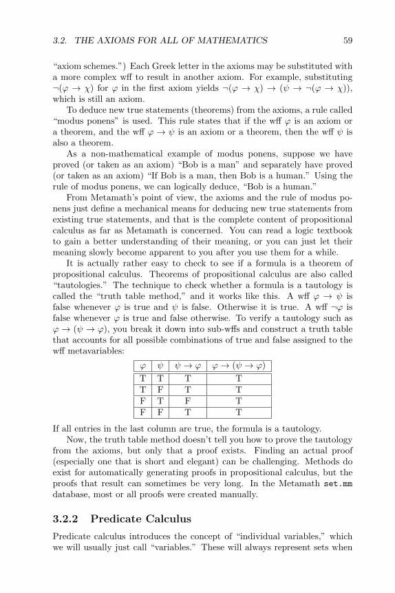
3.2. THE AXIOMS FOR ALL OF MATHEMATICS 59
“axiom schemes.”) Each Greek letter in the axioms may be substituted witha more complex wff to result in another axiom. For example, substituting¬(ϕ → χ) for ϕ in the first axiom yields ¬(ϕ → χ) → (ψ → ¬(ϕ → χ)),which is still an axiom.
To deduce new true statements (theorems) from the axioms, a rule called“modus ponens” is used. This rule states that if the wff ϕ is an axiom ora theorem, and the wff ϕ → ψ is an axiom or a theorem, then the wff ψ isalso a theorem.
As a non-mathematical example of modus ponens, suppose we haveproved (or taken as an axiom) “Bob is a man” and separately have proved(or taken as an axiom) “If Bob is a man, then Bob is a human.” Using therule of modus ponens, we can logically deduce, “Bob is a human.”
From Metamath’s point of view, the axioms and the rule of modus po-nens just define a mechanical means for deducing new true statements fromexisting true statements, and that is the complete content of propositionalcalculus as far as Metamath is concerned. You can read a logic textbookto gain a better understanding of their meaning, or you can just let theirmeaning slowly become apparent to you after you use them for a while.
It is actually rather easy to check to see if a formula is a theorem ofpropositional calculus. Theorems of propositional calculus are also called“tautologies.” The technique to check whether a formula is a tautology iscalled the “truth table method,” and it works like this. A wff ϕ → ψ isfalse whenever ϕ is true and ψ is false. Otherwise it is true. A wff ¬ϕ isfalse whenever ϕ is true and false otherwise. To verify a tautology such asϕ → (ψ → ϕ), you break it down into sub-wffs and construct a truth tablethat accounts for all possible combinations of true and false assigned to thewff metavariables:
ϕ ψ ψ → ϕ ϕ→ (ψ → ϕ)
T T T TT F T TF T F TF F T T
If all entries in the last column are true, the formula is a tautology.Now, the truth table method doesn’t tell you how to prove the tautology
from the axioms, but only that a proof exists. Finding an actual proof(especially one that is short and elegant) can be challenging. Methods doexist for automatically generating proofs in propositional calculus, but theproofs that result can sometimes be very long. In the Metamath set.mm
database, most or all proofs were created manually.
3.2.2 Predicate Calculus
Predicate calculus introduces the concept of “individual variables,” whichwe will usually just call “variables.” These will always represent sets when

60 CHAPTER 3. ABSTRACT MATHEMATICS REVEALED
we get to set theory. There are also three new symbols ∀, =, and ∈, read“for all,” “equals,” and “is an element of” respectively. We will representvariables with the letters x, y, z, and w, as is common practice in theliterature.
To prevent confusion, it might be best at this point to think of the vari-ables of Metamath as “metavariables,” because they are not quite the sameas the variables we are introducing here. A (meta)variable in Metamathcan be a wff or an individual variable, as well as many other things; in gen-eral, it represents a kind of place holder for an unspecified sequence of mathsymbols.
In predicate calculus, we extend the definition of a wff. If ϕ is a wff andx and y are variables, then ∀xϕ, x = y, and x ∈ y are wffs. Note thatthese three new types of wffs can be considered “starting” wffs from whichwe can build other wffs with → and ¬ . The concept of a starting wff wasabsent in propositional calculus. But starting wff or not, all we are reallyconcerned with is whether our wffs are correctly constructed according tothese mechanical rules.
In standard texts of logic, there are two axioms of predicate calculus:
∀xϕ(x)→ ϕ(y), where “y is properly substituted for x.”∀x(ϕ→ ψ)→ (ϕ→ ∀xψ), where “x is not free in ϕ.”
Now at first glance, this seems simple: just two axioms. However, condi-tional clauses are attached to each axiom describing requirements that mayseem puzzling to you. In addition, the first axiom puts a variable symbolin parentheses after each wff, seemingly violating our definition of a wff;this is just an informal way of referring to some arbitrary variable that mayoccur in the wff. The conditional clauses do, of course, have a precise mean-ing, but as it turns out the precise meaning is somewhat complicated andawkward to formalize in a way that a computer can handle easily. Unlikepropositional calculus, a certain amount of mathematical sophistication andpractice is needed to be able to easily grasp and manipulate these conceptscorrectly.
We take a different approach in the Metamath database set.mm. We donot use the primitive notions of “free variable” and “proper substitution” atall. Instead, we use a set of axioms that are almost as simple to manipulate asthose of propositional calculus. Our axiom system avoids complex primitivenotions by effectively embedding the complexity into the axioms themselves.As a result, we will end up with a larger number of axioms, but they areideally suited for a computer language such as Metamath. (Section 3.3 showsthese axioms.)
We will not elaborate on the “free variable” and “proper substitution”concepts here. We listed the two axioms above so that you will recognizethem when you encounter them in the literature. You may consult [19, ch. 3–4] (as well as many other books) for a precise explanation of these concepts.If you intend to do serious mathematical work, it is wise to become familiar

3.2. THE AXIOMS FOR ALL OF MATHEMATICS 61
with the traditional textbook approach; even though the concepts embeddedin their axioms require a higher level of sophistication, they can be morepractical to deal with on an everyday, informal basis. Even if you are justdeveloping Metamath proofs, familiarity with the traditional approach canhelp you arrive at a proof outline much faster, which you can then convertto the detail required by Metamath.
There is also a new rule of inference in predicate calculus: if ϕ is anaxiom or a theorem, then ∀xϕ is also a theorem. This is called the rule of“generalization.”
Unlike propositional calculus, no decision procedure analogous to thetruth table method exists (nor theoretically can exist) that will definitelydetermine whether a formula is a theorem of predicate calculus. Much ofthe work in the field of automated theorem proving has been dedicated tocoming up with clever heuristics for proving theorems of predicate calculus,but they can never be guaranteed to work always.
3.2.3 Equality
Predicate calculus may be presented with or without axioms for equality.We will require the axioms of equality as a prerequisite for the version ofset theory we will use. In standard systems, the axioms for equality are thefollowing two:
x = x
x = y → (ϕ(x, x)→ ϕ(x, y)) where “ϕ(x, y) arises from ϕ(x, x) byreplacing some, but not necessarily all, free occurrences of x by y,
provided that y is free for x in φ(x, x).”
The first equality axiom is simple, but the condition on the second one issomewhat awkward to implement on a computer. Again, the axiom systemwe use in the set.mm database avoids the complexity of this condition byeffectively embedding the complexity into the axioms themselves.
3.2.4 Set Theory
Traditional Zermelo-Fraenkel set theory has 10 axioms, which can be ex-pressed in the language of predicate calculus. In this section, we will listonly the names and brief English descriptions of these axioms, since we willgive you the precise formulas used by the Metamath set theory databaseset.mm later on.
In the descriptions of the axioms, we assume that x, y, z, w, and v rep-resent sets. These are the same as the variables in our predicate calculussystem above, except that now we informally think of the variables as rang-ing over sets. Note that the terms “object,” “set,” “element,” “collection,”and “family” are synonymous, as are “is an element of,” “is a member of,”

62 CHAPTER 3. ABSTRACT MATHEMATICS REVEALED
“is contained in,” and “belongs to.” The different terms are used for con-venience; for example, “a collection of sets” is less confusing than “a set ofsets.” A set x is said to be a “subset” of y if every element of x is also anelement of y; we also say x is “included in” y.
The axioms are very general and apply to almost any conceivable math-ematical object, and this level of abstraction can be overwhelming at first.To gain an intuitive feel, it can be helpful to draw a picture illustrating theconcept; for example, a circle containing dots could represent a collection ofsets, and a smaller circle drawn inside of the circle could represent a subset.Overlapping circles can illustrate intersection and union. Circles that illus-trate the concepts of set theory are frequently used in elementary textbooksand are called Venn diagrams.
1. Axiom of Extensionality: Two sets are identical if they contain thesame elements.
2. Axiom of Pairing: The set {x, y} exists.3. Axiom of Power Sets: The power set of a set (the collection of all of its
subsets) exists. For example, the power set of {x, y} is {∅, {x}, {y}, {x, y}}and it exists.
4. Axiom of the Null Set: The empty set ∅ exists.5. Axiom of Union: The union of a set (the set containing the elements
of its members) exists. For example, the union of {{x, y}, {z}} is {x, y, z}and it exists.
6. Axiom of Regularity: Roughly, no set can contain itself, nor canthere be membership “loops,” such as a set being an element of one of itsmembers.
7. Axiom of Infinity: An infinite set exists. An example of an infiniteset is the set of all integers.
8. Axiom of Separation: The set exists that is obtained by restricting xwith some property. For example, if the set of all integers exists, then theset of all even integers exists.
9. Axiom of Replacement: The range of a function whose domain isrestricted to the elements of a set x, is also a set. For example, there is afunction from integers (the function’s domain) to their squares (its range).If we restrict the domain to even integers, its range will become the set ofsquares of even integers, so this axioms asserts that the set of squares ofeven numbers exists. Technical note: In general, the “function” need not bea set but can be a proper class.
10. Axiom of Choice: Let x be a set whose members are pairwise disjoint(i.e, whose members contain no elements in common). Then there existsanother set containing one element from each member of x. For example, ifx is {{y, z}, {w, v}}, where y, z, w, and v are different sets, then a set suchas {z, w} exists (but the axiom doesn’t tell us which one). (Actually theAxiom of Choice is redundant if the set x, as in this example, has a finitenumber of elements.)

3.3. THE AXIOMS IN THE METAMATH LANGUAGE 63
The Axiom of Choice is usually considered an extension of ZF set theoryrather than a proper part of it. It is sometimes considered philosophicallycontroversial because it specifies the existence of a set without specifyingwhat the set is. ZF set theory that includes the Axiom of Choice is calledZFC.
When expressed symbolically, the Axiom of Separation and the Axiomof Replacement contain wff symbols and therefore each represent infinitelymany axioms, one for each possible wff. For this reason, they are often calledaxiom schemes.
It turns out that the Axiom of the Null Set, the Axiom of Pairing, and theAxiom of Separation can be derived from the other axioms and are thereforeunnecessary, although they tend to be included in standard texts for variousreasons (historical, philosophical, and possibly because some authors maynot know this). In the Metamath set theory database, these redundantaxioms are derived from the other ones.
3.3 The Axioms in the Metamath Language
The standard textbook axioms of predicate calculus are somewhat cumber-some to implement on a computer because of the complex notions of “freevariable” and “proper substitution.” While it is possible to use the Meta-math language to implement these concepts, we have chosen not to do soin the set.mm set theory database. Instead, we have eliminated them bycarefully crafting the axioms so as to avoid them. This makes it easy for abeginner to follow the steps in a proof without knowing any advanced con-cepts other than the simple concept of replacing variables with expressions.Here we list the axioms as they appear in set.mm so you can look them upthere easily. Incidentally, the show statement /tex command was used totypeset them.
In order to develop the concepts of free variable and proper substitutionfrom the axioms described below, we use an additional Metamath statementtype called “disjoint variable restriction” that we have not encountered be-fore. In the context of the axioms, the statement $d x y simply means thatx and y must be distinct, i.e. they may not be simultaneously substitutedwith the same variable. The statement $d xϕ means variable x must notoccur in wff ϕ. For the precise definition of $d, see Section 4.2.4.
In our system, the axioms of predicate calculus have been divided intowhat we call “pure predicate calculus,” which uses no = or ∈ symbols, and“equality and substitution.” The former is weaker than traditional predicatecalculus because it does not have substitution (although it is a beautifullysimple and interesting system in itself), and the latter extends its power tothe full predicate calculus with equality.
You should also note that our system of predicate calculus is specificallytailored for set theory; thus there are only two specific predicates = and ∈

64 CHAPTER 3. ABSTRACT MATHEMATICS REVEALED
and no functions or constants unlike more general systems.Finally, I do not claim that these axioms are the most elegant possible.
They have more “metalogical” power than standard axioms (although theyare equivalent in a “logical” sense) and the ones I have chosen at least dothe job. Perhaps a logician who reads this would be interested in devisinga set of equivalent axioms that are shorter or more elegant in some sense.(For example, there used to be an axiom ax-15 in our list that was later dis-covered to be redundant in this version of the axiom system. The Commenton p. 105 has a further remark on this axiom.)
A rigorous justification for this system can be found in [34].
3.3.1 Propositional Calculus
Axiom of Simplification.ax-1 $a ` (ϕ→ (ψ→ϕ ) )
Axiom of Distribution.ax-2 $a ` ( (ϕ→ (ψ→χ ) )→ ( (ϕ→ψ )→ (ϕ→χ ) ) )
Axiom of Contraposition.ax-3 $a ` ( (¬ϕ→¬ψ )→ (ψ→ϕ ) )
Rule of Modus Ponens.maj $e ` (ϕ→ψ )min $e `ϕax-mp $a `ψ
3.3.2 Pure Predicate Calculus
Axiom of Specialization.ax-4 $a ` (∀xϕ→ϕ )
Axiom of Quantified Implication.ax-5 $a ` (∀x (∀xϕ→ψ )→ (∀xϕ→∀xψ ) )
Axiom of Quantified Negation.ax-6 $a ` (¬∀x¬∀xϕ→ϕ )
Axiom of Quantifier Commutation.ax-7 $a ` (∀x∀ y ϕ→∀ y ∀xϕ )
Rule of Generalization.ax-g.1 $e `ϕax-gen $a `∀xϕ
3.3.3 Equality and Substitution
Axiom of Equality (1).ax-8 $a ` (x= y→ (x= z→ y= z ) )
Axiom of Existence.ax-9 $a ` (∀x (x= y→∀xϕ )→ϕ )
Axiom of Quantifier Substitution.
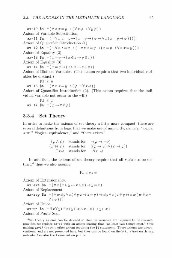
3.3. THE AXIOMS IN THE METAMATH LANGUAGE 65
ax-10 $a ` (∀x x= y→ (∀xϕ→∀ y ϕ ) )Axiom of Variable Substitution.ax-11 $a ` (¬∀x x= y→ (x= y→ (ϕ→∀x (x= y→ϕ ) ) ) )
Axiom of Quantifier Introduction (1).ax-12 $a ` (¬∀ z z=x→ (¬∀ z z= y→ (x= y→∀ z x= y ) ) )
Axiom of Equality (2).ax-13 $a ` (x= y→ (x∈ z→ y ∈ z ) )
Axiom of Equality (3).ax-14 $a ` (x= y→ ( z ∈x→ z ∈ y ) )
Axiom of Distinct Variables. (This axiom requires that two individual vari-ables be distinct.)
$d x yax-16 $a ` (∀x x= y→ (ϕ→∀xϕ ) )
Axiom of Quantifier Introduction (2). (This axiom requires that the indi-vidual variable not occur in the wff.)
$d x ϕax-17 $a ` (ϕ→∀xϕ )
3.3.4 Set Theory
In order to make the axioms of set theory a little more compact, there areseveral definitions from logic that we make use of implicitly, namely, “logicaland,” “logical equivalence,” and “there exists.”
(ϕ ∧ ψ) stands for ¬(ϕ→ ¬ψ)(ϕ↔ ψ) stands for ((ϕ→ ψ) ∧ (ψ → ϕ))∃xϕ stands for ¬∀x¬ϕ
In addition, the axioms of set theory require that all variables be dis-tinct,4 thus we also assume:
$d x y z w
Axiom of Extensionality.ax-ext $a ` (∀x (x∈ y↔x∈ z )→ y= z )
Axiom of Replacement.ax-rep $a ` (∀w ∃ y ∀ z (∀ y ϕ→ z= y )→∃ y ∀ z ( z ∈ y↔∃w (w∈x∧
∀ y ϕ ) ) )Axiom of Union.ax-un $a `∃x∀ y (∃x ( y ∈x∧x∈ z )→ y ∈x )
Axiom of Power Sets.
4Set theory axioms can be devised so that no variables are required to be distinct,provided we replace ax-16 with an axiom stating that “at least two things exist,” thusmaking ax-17 the only other axiom requiring the $d statement. These axioms are uncon-ventional and are not presented here, but they can be found on the http://metamath.org
web site. See also the Comment on p. 105.

66 CHAPTER 3. ABSTRACT MATHEMATICS REVEALED
ax-pow $a `∃x∀ y (∀x (x∈ y→x∈ z )→ y ∈x )Axiom of Regularity.ax-reg $a ` (∃x x∈ y→∃x (x∈ y ∧∀ z ( z ∈x→¬ z ∈ y ) ) )
Axiom of Infinity.ax-inf $a `∃x ( y ∈x∧∀ y ( y ∈x→∃ z ( y ∈ z ∧ z ∈x ) ) )
Axiom of Choice.ax-ac $a `∃x∀ y ∀ z ( ( y ∈ z ∧ z ∈w )→∃w ∀ y (∃w ( ( y ∈ z ∧ z ∈w )∧ (
y ∈w∧w∈x ) )↔ y=w ) )
3.3.5 That’s It
There you have it, the axioms for (essentially) all of mathematics! Wonderat them and stare at them in awe. Put a copy in your wallet, and you willcarry in your pocket the encoding for all theorems ever proved and that everwill be proved, from the most mundane to the most profound.
3.4 A Hierarchy of Definitions
The axioms in the previous section in principle embody everything that canbe done within standard mathematics. However, it is impractical to accom-plish very much by using them directly, for even simple concepts (from ahuman perspective) can involve extremely long, incomprehensible formulas.Mathematics is made practical by introducing definitions. Definitions usu-ally introduce new symbols, or at least new relationships among existingsymbols, to abbreviate more complex formulas. An important requirementfor a definition is that there exist a straightforward (algorithmic) methodfor eliminating the abbreviation by expanding it into the more primitivesymbol string that it represents. Some important definitions included in thefile set.mm are listed in this section for reference, and also to give you a feelfor why something like ω (the set of natural numbers 0, 1, 2,. . . ) becomesvery complicated when completely expanded into primitive symbols.
What is the motivation for definitions, aside from allowing complicatedexpressions to be expressed more simply? In the case of ω, one goal isto provide a basis for the theory of natural numbers. Before set theorywas invented, a set of axioms for arithmetic, called Peano’s postulates, wasdevised and shown to have the properties one expects for natural numbers.Now anyone can postulate a set of axioms, but if the axioms are inconsistentcontradictions can be derived from them. Once a contradiction is derived,anything can be trivially proved, including all the facts of arithmetic andtheir negations. To ensure that an axiom system is at least as reliable asthe axioms for set theory, we can define sets and operations on those setsthat satisfy the new axioms. In the set.mm Metamath database, we provethat the elements of ω satisfy Peano’s postulates, and it’s a long and hardjourney to get there directly from the axioms of set theory. But the result is

3.4. A HIERARCHY OF DEFINITIONS 67
confidence in the foundations of arithmetic. And there is another advantage:we now have all the tools of set theory at our disposal for manipulatingobjects that obey the axioms for arithmetic.
What are the criteria we use for definitions? First, and of utmost impor-tance, the definition should not be creative, that is it should not allow anexpression that previously qualified as a wff but was not provable, to becomeprovable. Second, the definition should be eliminable, that is there shouldexist an algorithmic method for proving any expression using the definitioninto a logically equivalent expression that previously qualified as a wff.
In almost all cases below, definitions connect two expressions with either↔ or =. Eliminating5 such a definition is a simple matter of substituting theexpression on the left-hand side (definiendum or thing being defined) withthe equivalent, more primitive expression on the right-hand side (definiensor definition).
Often a definition has variables on the right-hand side which do not ap-pear on the left-hand side; these are called dummy variables. In this case,any allowable substitution (such as a new, distinct variable) can be usedwhen the definition is eliminated. Dummy variables may be used only ifthey are effectively bound, meaning that the definition will remain logicallyequivalent upon any substitution of a dummy variable with any other quali-fying expression, i.e. any symbol string (such as another variable) that meetsthe restrictions on the dummy variable imposed by $d and $f statements.For example, we could define a constant ⊥ (inverted tee, meaning logical“false”) as (ϕ ∧ ¬ϕ), i.e. “phi and not phi.” Here ϕ is effectively boundbecause the definition remains logically equivalent when we replace ϕ withany other wff. (We do not define ⊥ in set.mm.)
There are two cases where eliminating definitions is a little more complex.These cases are the definitions df-bi and df-cleq. The first stretches theconcept of a definition a little, as in effect it “defines a definition;” however,it meets our requirements for a definition in that it is eliminable and doesnot strengthen the language. Theorem bii shows the substitution neededto eliminate the ↔ symbol.
Definition df-cleq extends the usage of the equality symbol to include“classes” in set theory. The reason it is potentially problematic is that it canlead to statements which do not follow from logic alone but presuppose theAxiom of Extensionality, so we include this axiom as a hypothesis for thedefinition. We could have made df-cleq directly eliminable by introducinga new equality symbol, but have chosen not to do so in keeping with standardtextbook practice. Definitions such as df-cleq that extend the meaning ofexisting symbols must be introduced carefully so that they do not lead tocontradictions. Definition df-clel also extends the meaning of an existing
5Here we mean the elimination that a human might do in his or her head. To eliminatethem as part of a Metamath proof we would invoke one of a number of theorems that dealwith transitivity of equivalence or equality; there are many such examples in the proofsin set.mm.

68 CHAPTER 3. ABSTRACT MATHEMATICS REVEALED
symbol (∈); while it doesn’t strengthen the language like df-cleq, this isnot obvious and it must also be subject to the same scrutiny.
Exercise: Study how the wff x ∈ ω, meaning “x is a natural number,”could be expanded in terms of primitive symbols, starting with the defini-tions df-clel on p. 71 and df-om on p. 74 and working your way back.Don’t bother to work out the details; just make sure that you understandhow you could do it in principle. The answer is shown in the footnote onp. 57. If you actually do work it out, you won’t get exactly the same answerbecause we used a few simplifications such as discarding occurrences of ¬¬(double negation).
In the definitions below, we have placed the ascii Metamath sourcebelow each of the formulas to help you to become familiar with the notationin the database. For simplicity, the necessary $f and $d statements arenot shown. If you are in doubt, use the show statement command in theMetamath program to see the full statement.
To understand the motivation for these definitions, you should consultthe references indicated: Takeuti and Zaring [59], Quine [48], Bell and Ma-chover [5], and Enderton [16]. Our list of definitions is provided more forreference than as a learning aid. However, by looking at a few of them youcan gain a feel for how the hierarchy is built up. The definitions are a rep-resentative sample of the 130 or so in set.mm, but they are complete withrespect to the theorem examples we will present in Section 3.6. Also, someare slightly different from, but logically equivalent to, the ones in set.mm
(some of which have been revised over time to shorten them, for example).
3.4.1 Definitions for Propositional Calculus
The symbols ϕ, ψ, and χ represent wffs.Our first definition introduces the biconditional connective6 (also called
logical equivalence). Unlike most traditional developments, we have chosennot to have a separate symbol such as “Df.” to mean “is defined as.” Instead,we will use the biconditional connective for this purpose, as it lets us uselogic to manipulate definitions directly. Here we state the properties ofthe biconditional connective with a carefully crafted $a statement, whicheffectively uses the biconditional connective to define itself. The ↔ symbolcan be eliminated from a formula using theorem bii, which is derived later.
Define the biconditional connective.
df-bi $a `¬ ( ( (ϕ↔ψ )→¬ ( (ϕ→ψ )→¬ (ψ→ϕ ) ) )→¬ (¬ ( (ϕ→ψ )→¬ (ψ→ϕ ) )→ (ϕ↔ψ ) ) )
6The term “connective” is informally used to mean a symbol that is placed between twovariables or adjacent to a variable, whereas a mathematical “constant” usually indicatesa symbol such as the number 0 that may replace a variable or metavariable. FromMetamath’s point of view, there is no distinction between a connective and a constant;both are constants in the Metamath language.

3.4. A HIERARCHY OF DEFINITIONS 69
df-bi $a |- -. ( ( ( ph <-> ps ) -> -. ( ( ph -> ps ) ->
-. ( ps -> ph ) ) ) -> -. ( -. ( ( ph -> ps ) -> -. (
ps -> ph ) ) -> ( ph <-> ps ) ) ) $.
This theorem relates the biconditional connective to primitive connectivesand can be used to eliminate the ↔ symbol from any wff.
bii $p ` ( (ϕ↔ψ )↔¬ ( (ϕ→ψ )→¬ (ψ→ϕ ) ) )bii $p |- ( ( ph <-> ps ) <-> -. ( ( ph -> ps ) -> -. ( ps
-> ph ) ) ) $= ... $.
Define disjunction (or).
df-or $a ` ( (ϕ∨ψ )↔ (¬ϕ→ψ ) )df-or $a |- ( ( ph \/ ps ) <-> ( -. ph -> ps ) ) $.
Define conjunction (and).
df-an $a ` ( (ϕ∧ψ )↔¬ (ϕ→¬ψ ) )df-an $a |- ( ( ph /\ ps ) <-> -. ( ph -> -. ps ) ) $.
Define disjunction (or) of 3 wffs.
df-3or $a ` ( (ϕ∨ψ ∨χ )↔ ( (ϕ∨ψ )∨χ ) )df-3or $a |- ( ( ph \/ ps \/ ch ) <-> ( ( ph \/ ps ) \/ ch
) ) $.
Define conjunction (and) of 3 wffs.
df-3an $a ` ( (ϕ∧ψ ∧χ )↔ ( (ϕ∧ψ )∧χ ) )df-3an $a |- ( ( ph /\ ps /\ ch ) <-> ( ( ph /\ ps ) /\ ch
) ) $.
3.4.2 Definitions for Predicate Calculus
The symbols x, y, and z represent individual variables of predicate calcu-lus. In this section, they are not necessarily distinct unless it is explicitlymentioned.
Define existential quantification.
df-ex $a ` (∃xϕ↔¬∀x¬ϕ )df-ex $a |- ( E. x ph <-> -. A. x -. ph ) $.
Define proper substitution. Note that this definition is valid even when xand y are the same variable. The first conjunct is a “trick” used to achievethis property, making the definition look somewhat peculiar at first. For ournotation, we use [y/x]ϕ to mean “the wff that results when y is properlysubstituted with x in the wff ϕ.” The notation is different from the notationϕ(x|y) that is sometimes used, because the latter notation is ambiguous forus: for example, we don’t know whether ¬ϕ(x|y) is to be interpreted as
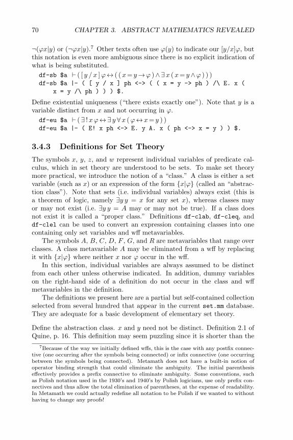
70 CHAPTER 3. ABSTRACT MATHEMATICS REVEALED
¬(ϕx|y) or (¬ϕx|y).7 Other texts often use ϕ(y) to indicate our [y/x]ϕ, butthis notation is even more ambiguous since there is no explicit indication ofwhat is being substituted.
df-sb $a ` ( [ y / x ]ϕ↔ ( (x= y→ϕ )∧∃x (x= y ∧ϕ ) ) )df-sb $a |- ( [ y / x ] ph <-> ( ( x = y -> ph ) /\ E. x (
x = y /\ ph ) ) ) $.
Define existential uniqueness (“there exists exactly one”). Note that y is avariable distinct from x and not occurring in ϕ.
df-eu $a ` (∃ !xϕ↔∃ y ∀x (ϕ↔x= y ) )df-eu $a |- ( E! x ph <-> E. y A. x ( ph <-> x = y ) ) $.
3.4.3 Definitions for Set Theory
The symbols x, y, z, and w represent individual variables of predicate cal-culus, which in set theory are understood to be sets. To make set theorymore practical, we introduce the notion of a “class.” A class is either a setvariable (such as x) or an expression of the form {x|ϕ} (called an “abstrac-tion class”). Note that sets (i.e. individual variables) always exist (this isa theorem of logic, namely ∃y y = x for any set x), whereas classes mayor may not exist (i.e. ∃y y = A may or may not be true). If a class doesnot exist it is called a “proper class.” Definitions df-clab, df-cleq, anddf-clel can be used to convert an expression containing classes into onecontaining only set variables and wff metavariables.
The symbols A, B, C, D, F , G, and R are metavariables that range overclasses. A class metavariable A may be eliminated from a wff by replacingit with {x|ϕ} where neither x nor ϕ occur in the wff.
In this section, individual variables are always assumed to be distinctfrom each other unless otherwise indicated. In addition, dummy variableson the right-hand side of a definition do not occur in the class and wffmetavariables in the definition.
The definitions we present here are a partial but self-contained collectionselected from several hundred that appear in the current set.mm database.They are adequate for a basic development of elementary set theory.
Define the abstraction class. x and y need not be distinct. Definition 2.1 ofQuine, p. 16. This definition may seem puzzling since it is shorter than the
7Because of the way we initially defined wffs, this is the case with any postfix connec-tive (one occurring after the symbols being connected) or infix connective (one occurringbetween the symbols being connected). Metamath does not have a built-in notion ofoperator binding strength that could eliminate the ambiguity. The initial parenthesiseffectively provides a prefix connective to eliminate ambiguity. Some conventions, suchas Polish notation used in the 1930’s and 1940’s by Polish logicians, use only prefix con-nectives and thus allow the total elimination of parentheses, at the expense of readability.In Metamath we could actually redefine all notation to be Polish if we wanted to withouthaving to change any proofs!

3.4. A HIERARCHY OF DEFINITIONS 71
expression being defined and does not buy us anything in terms of brevity.The reason we introduce this definition is because it fits in neatly with theextension of the ∈ connective provided by df-clel.
df-clab $a ` (x∈{ y |ϕ }↔ [x / y ]ϕ )df-clab $a |- ( x e. { y | ph } <-> [ x / y ] ph ) $.
Define the equality connective between classes. See Quine or Chapter 4 ofTakeuti and Zaring for its justification and methods for eliminating it. Thisis an example of a somewhat “dangerous” definition, because it extends theuse of the existing equality symbol rather than introducing a new symbol,allowing us to make statements in the original language that may not betrue. For example, it permits us to deduce y = z ↔ ∀x(x ∈ y ↔ x ∈ z)which is not a theorem of logic but rather presupposes the Axiom of Exten-sionality, which we include as a hypothesis so that we can know when thisaxiom is assumed in a proof (with the show trace_back command). Wecould avoid the danger by introducing another symbol, say P, in place of=; this would also have the advantage of making elimination of the defini-tion straightforward and would eliminate the need for Extensionality as ahypothesis. We would then also have the advantage of being able to identifyexactly where Extensionality truly comes into play. One of our theoremswould be x P y ↔ x = y by invoking Extensionality. However in keepingwith standard practice we retain the “dangerous” definition.
df-cleq.1 $e ` (∀x (x∈ y↔x∈ z )→ y= z )df-cleq $a ` (A=B↔∀x (x∈A↔x∈B ) )
df-cleq.1 $e |- ( A. x ( x e. y <-> x e. z ) -> y = z ) $.
df-cleq $a |- ( A = B <-> A. x ( x e. A <-> x e. B ) ) $.
Define the membership connective between classes. Theorem 6.3 of Quine,p. 41, which we adopt as a definition. Note that it extends the use of theexisting membership symbol, but unlike df-cleq it does not extend theset of valid wffs of logic when the class metavariables are replaced with setvariables.
df-clel $a ` (A∈B↔∃x (x=A∧x∈B ) )df-clel $a |- ( A e. B <-> E. x ( x = A /\ x e. B ) ) $.
Define inequality.
df-ne $a ` (A 6=B↔¬A=B )df-ne $a |- ( A =/= B <-> -. A = B ) $.
Define restricted universal quantification. Enderton, p. 22.
df-ral $a ` (∀x∈Aϕ↔∀x (x∈A→ϕ ) )df-ral $a |- ( A. x e. A ph <-> A. x ( x e. A -> ph ) ) $.
Define restricted existential quantification. Enderton, p. 22.
df-rex $a ` (∃x∈Aϕ↔∃x (x∈A∧ϕ ) )df-rex $a |- ( E. x e. A ph <-> E. x ( x e. A /\ ph ) ) $.

72 CHAPTER 3. ABSTRACT MATHEMATICS REVEALED
Define the universal class. Definition 5.20, p. 21, of Takeuti and Zaring.
df-v $a `V = {x |x=x }df-v $a |- V = { x | x = x } $.
Define the subclass relationship between two classes (called the subset rela-tion if the classes are sets i.e. are not proper). Definition 5.9 of Takeuti andZaring, p. 17.
df-ss $a ` (A⊆B↔∀x (x∈A→x∈B ) )df-ss $a |- ( A (_ B <-> A. x ( x e. A -> x e. B ) ) $.
Define the union of two classes. Definition 5.6 of Takeuti and Zaring, p. 16.
df-un $a ` (A∪B ) = {x | (x∈A∨x∈B ) }df-un $a |- ( A u. B ) = { x | ( x e. A \/ x e. B ) } $.
Define the intersection of two classes. Definition 5.6 of Takeuti and Zaring,p. 16.
df-in $a ` (A∩B ) = {x | (x∈A∧x∈B ) }df-in $a |- ( A i^i B ) = { x | ( x e. A /\ x e. B ) } $.
Define class difference. Definition 5.12 of Takeuti and Zaring, p. 20. Severalnotations are used in the literature; we chose the \ convention instead of aminus sign to reserve the latter for later use in, e.g., arithmetic.
df-dif $a ` (A \B ) = {x | (x∈A∧¬x∈B ) }df-dif $a |- ( A \ B ) = { x | ( x e. A /\ -. x e. B ) } $.
Define the empty or null set. Compare Definition 5.14 of Takeuti and Zaring,p. 20.
df-nul $a `∅= (V \V )df-nul $a |- (/) = ( V \ V ) $.
Define power class. Definition 5.10 of Takeuti and Zaring, p. 17, but we alsolet it apply to proper classes. (Note that P~ is the symbol for calligraphicP, the tilde suggesting “curly;” see Appendix A.)
df-pw $a `P A= {x |x⊆A }df-pw $a |- P~ A = { x | x (_ A } $.
Define the singleton of a class. Definition 7.1 of Quine, p. 48. It is well-defined for proper classes, although it is not very meaningful in this case,where it evaluates to the empty set.
df-sn $a ` {A }= {x |x=A }df-sn $a |- { A } = { x | x = A } $.
Define an unordered pair of classes. Definition 7.1 of Quine, p. 48.
df-pr $a ` {A ,B }= ( {A }∪ {B } )df-pr $a |- { A , B } = ( { A } u. { B } ) $.
Define an unordered triple of classes. Definition of Enderton, p. 19.
df-tp $a ` {A ,B ,C }= ( {A ,B }∪ {C } )
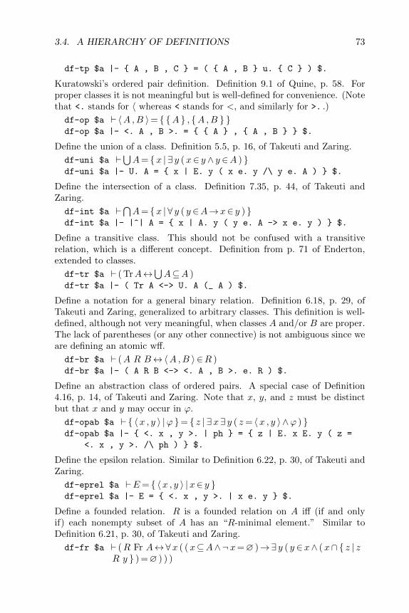
3.4. A HIERARCHY OF DEFINITIONS 73
df-tp $a |- { A , B , C } = ( { A , B } u. { C } ) $.
Kuratowski’s ordered pair definition. Definition 9.1 of Quine, p. 58. Forproper classes it is not meaningful but is well-defined for convenience. (Notethat <. stands for 〈 whereas < stands for <, and similarly for >. .)
df-op $a ` 〈A ,B 〉= { {A } , {A ,B } }df-op $a |- <. A , B >. = { { A } , { A , B } } $.
Define the union of a class. Definition 5.5, p. 16, of Takeuti and Zaring.
df-uni $a `⋃A= {x | ∃ y (x∈ y ∧ y ∈A ) }
df-uni $a |- U. A = { x | E. y ( x e. y /\ y e. A ) } $.
Define the intersection of a class. Definition 7.35, p. 44, of Takeuti andZaring.
df-int $a `⋂A= {x | ∀ y ( y ∈A→x∈ y ) }
df-int $a |- |^| A = { x | A. y ( y e. A -> x e. y ) } $.
Define a transitive class. This should not be confused with a transitiverelation, which is a different concept. Definition from p. 71 of Enderton,extended to classes.
df-tr $a ` ( TrA↔⋃A⊆A )
df-tr $a |- ( Tr A <-> U. A (_ A ) $.
Define a notation for a general binary relation. Definition 6.18, p. 29, ofTakeuti and Zaring, generalized to arbitrary classes. This definition is well-defined, although not very meaningful, when classes A and/or B are proper.The lack of parentheses (or any other connective) is not ambiguous since weare defining an atomic wff.
df-br $a ` (A R B↔〈A ,B 〉 ∈R )df-br $a |- ( A R B <-> <. A , B >. e. R ) $.
Define an abstraction class of ordered pairs. A special case of Definition4.16, p. 14, of Takeuti and Zaring. Note that x, y, and z must be distinctbut that x and y may occur in ϕ.
df-opab $a ` { 〈x , y 〉 |ϕ }= { z | ∃x ∃ y ( z= 〈x , y 〉 ∧ϕ ) }df-opab $a |- { <. x , y >. | ph } = { z | E. x E. y ( z =
<. x , y >. /\ ph ) } $.
Define the epsilon relation. Similar to Definition 6.22, p. 30, of Takeuti andZaring.
df-eprel $a `E= { 〈x , y 〉 |x∈ y }df-eprel $a |- E = { <. x , y >. | x e. y } $.
Define a founded relation. R is a founded relation on A iff (if and onlyif) each nonempty subset of A has an “R-minimal element.” Similar toDefinition 6.21, p. 30, of Takeuti and Zaring.
df-fr $a ` (R Fr A↔∀x ( (x⊆A∧¬x=∅ )→∃ y ( y ∈x∧ (x∩{ z | zR y } ) =∅ ) ) )
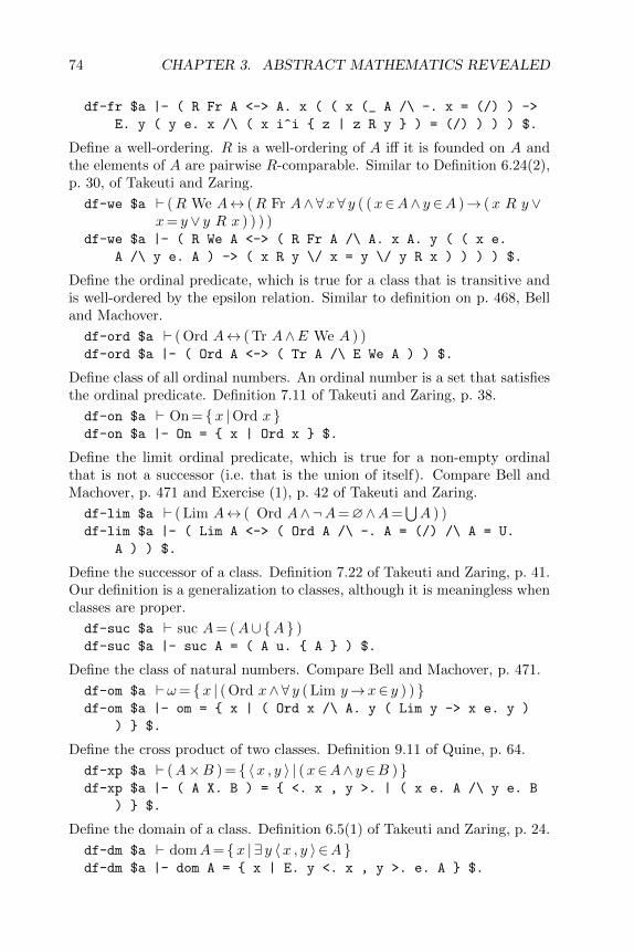
74 CHAPTER 3. ABSTRACT MATHEMATICS REVEALED
df-fr $a |- ( R Fr A <-> A. x ( ( x (_ A /\ -. x = (/) ) ->
E. y ( y e. x /\ ( x i^i { z | z R y } ) = (/) ) ) ) $.
Define a well-ordering. R is a well-ordering of A iff it is founded on A andthe elements of A are pairwise R-comparable. Similar to Definition 6.24(2),p. 30, of Takeuti and Zaring.
df-we $a ` (R We A↔ (R Fr A∧∀x∀ y ( (x∈A∧ y ∈A )→ (x R y ∨x= y ∨ y R x ) ) ) )
df-we $a |- ( R We A <-> ( R Fr A /\ A. x A. y ( ( x e.
A /\ y e. A ) -> ( x R y \/ x = y \/ y R x ) ) ) ) $.
Define the ordinal predicate, which is true for a class that is transitive andis well-ordered by the epsilon relation. Similar to definition on p. 468, Belland Machover.
df-ord $a ` ( Ord A↔ ( Tr A∧E We A ) )df-ord $a |- ( Ord A <-> ( Tr A /\ E We A ) ) $.
Define class of all ordinal numbers. An ordinal number is a set that satisfiesthe ordinal predicate. Definition 7.11 of Takeuti and Zaring, p. 38.
df-on $a ` On = {x |Ord x }df-on $a |- On = { x | Ord x } $.
Define the limit ordinal predicate, which is true for a non-empty ordinalthat is not a successor (i.e. that is the union of itself). Compare Bell andMachover, p. 471 and Exercise (1), p. 42 of Takeuti and Zaring.
df-lim $a ` ( Lim A↔ ( Ord A∧¬A=∅∧A=⋃A ) )
df-lim $a |- ( Lim A <-> ( Ord A /\ -. A = (/) /\ A = U.
A ) ) $.
Define the successor of a class. Definition 7.22 of Takeuti and Zaring, p. 41.Our definition is a generalization to classes, although it is meaningless whenclasses are proper.
df-suc $a ` suc A= (A∪{A } )df-suc $a |- suc A = ( A u. { A } ) $.
Define the class of natural numbers. Compare Bell and Machover, p. 471.
df-om $a `ω= {x | ( Ord x∧∀ y ( Lim y→x∈ y ) ) }df-om $a |- om = { x | ( Ord x /\ A. y ( Lim y -> x e. y )
) } $.
Define the cross product of two classes. Definition 9.11 of Quine, p. 64.
df-xp $a ` (A×B ) = { 〈x , y 〉 | (x∈A∧ y ∈B ) }df-xp $a |- ( A X. B ) = { <. x , y >. | ( x e. A /\ y e. B
) } $.
Define the domain of a class. Definition 6.5(1) of Takeuti and Zaring, p. 24.
df-dm $a ` domA= {x | ∃ y 〈x , y 〉 ∈A }df-dm $a |- dom A = { x | E. y <. x , y >. e. A } $.

3.4. A HIERARCHY OF DEFINITIONS 75
Define the range of a class. Definition 6.5(2) of Takeuti and Zaring, p. 24.
df-rn $a ` ranA= { y | ∃x 〈x , y 〉 ∈A }df-rn $a |- ran A = { y | E. x <. x , y >. e. A } $.
Define the restriction of a class. Definition 6.6(1) of Takeuti and Zaring,p. 24.
df-res $a ` (A �B ) = (A∩ (B×V ) )df-res $a |- ( A |‘ B ) = ( A i^i ( B X. V ) ) $.
Define the image of a class. Definition 6.6(2) of Takeuti and Zaring, p. 24.
df-ima $a ` (A “B ) = ran (A �B )df-ima $a |- ( A " B ) = ran ( A |‘ B ) $.
Define the composition of two classes. Definition 6.6(3) of Takeuti andZaring, p. 24.
df-co $a ` (A ◦B ) = { 〈x , y 〉 | ∃ z ( 〈x , z 〉 ∈B ∧ 〈 z , y 〉 ∈A ) }df-co $a |- ( A o. B ) = { <. x , y >. | E. z ( <. x , z
>. e. B /\ <. z , y >. e. A ) } $.
Define a relation. Definition 6.4(1) of Takeuti and Zaring, p. 23.
df-rel $a ` ( Rel A↔A⊆ (V ×V ) )df-rel $a |- ( Rel A <-> A (_ ( V X. V ) ) $.
Define a function. Definition 6.4(4) of Takeuti and Zaring, p. 24.
df-fun $a ` ( Fun A↔ ( Rel A∧∀x ∃ z ∀ y ( 〈x , y 〉 ∈A→ y= z ) ) )df-fun $a |- ( Fun A <-> ( Rel A /\ A. x E. z A. y ( <. x
, y >. e. A -> y = z ) ) ) $.
Define a function with domain. Definition 6.15(1) of Takeuti and Zaring,p. 27.
df-fn $a ` (A Fn B↔ ( Fun A∧dom A=B ) )df-fn $a |- ( A Fn B <-> ( Fun A /\ dom A = B ) ) $.
Define a function with domain and co-domain. Definition 6.15(3) of Takeutiand Zaring, p. 27.
df-f $a ` (F :A−→B↔ (F Fn A∧ ran F ⊆B ) )df-f $a |- ( F : A --> B <-> ( F Fn A /\ ran F (_ B ) ) $.
Define a one-to-one function. Compare Definition 6.15(5) of Takeuti andZaring, p. 27.
df-f1 $a ` (F :A1-1−→ B↔ (F :A−→B ∧∀ y ∃ z ∀x ( 〈x , y 〉 ∈F →x=
z ) ) )df-f1 $a |- ( F : A -1-1-> B <-> ( F : A --> B /\
A. y E. z A. x ( <. x , y >. e. F -> x = z ) ) ) $.
Define an onto function. Definition 6.15(4) of Takeuti and Zaring, p. 27.
df-fo $a ` (F :A −→onto B↔ (F Fn A∧ ran F =B ) )
df-fo $a |- ( F : A -onto-> B <-> ( F Fn A /\ ran F

76 CHAPTER 3. ABSTRACT MATHEMATICS REVEALED
= B ) ) $.
Define a one-to-one, onto function. Compare Definition 6.15(6) of Takeutiand Zaring, p. 27.
df-f1o $a ` (F :A1-1−→
onto B↔ (F :A1-1−→ B ∧F :A −→onto B ) )
df-f1o $a |- ( F : A -1-1-onto-> B <-> ( F : A -1-1-> B
/\ F : A -onto-> B ) ) $.
Define the value of a function. This definition applies to any class andevaluates to the empty set when it is not meaningful. Note that F ‘A meansthe same thing as the more familiar F (A) notation for a function’s value atA. The F ‘A notation is common in formal set theory.
df-fv $a ` (F ‘A ) =⋃{x | (F “ {A } ) = {x } }
df-fv $a |- ( F ‘ A ) = U. { x | ( F " { A } ) = { x } } $.
Define the result of an operation. Here, F is an operation on two values(such as + for real numbers). This is defined for proper classes A and Beven though not meaningful in that case. However, the definition can bemeaningful when F is a proper class.
df-opr $a ` (A F B ) = (F ‘ 〈A ,B 〉 )df-opr $a |- ( A F B ) = ( F ‘ <. A , B >. ) $.
3.5 Tricks of the Trade
In the set.mm database our goal was usually to conform to modern notation.However in some cases the relationship to standard textbook language maybe obscured by several unconventional devices we used to simplify the de-velopment and to take advantage of the Metamath language. In this sectionwe will describe some common conventions used in set.mm.
• The turnstile symbol, `, meaning “it is provable that,” is the first tokenof all assertions and hypotheses that aren’t syntax constructions. Thisis a standard convention in logic. (We mentioned this earlier, but thissymbol is bothersome to some people without a logic background. Ithas no deeper meaning but just provides us with a way to distinguishsyntax constructions from ordinary mathematical statements.)
• A hypothesis of the form
$e ` (ϕ→∀xϕ )
should be read “assume variable x is (effectively) not free in wff ϕ.”Literally, this says “assume it is provable that ϕ→ ∀xϕ.” This devicelets us avoid the complexities associated with the standard treatmentof free and bound variables. The footnote on p. 170 discusses thisfurther.
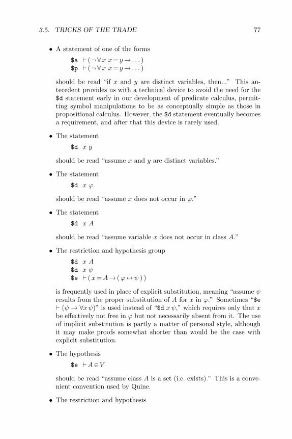
3.5. TRICKS OF THE TRADE 77
• A statement of one of the forms
$a ` (¬∀x x= y→ . . . )$p ` (¬∀x x= y→ . . . )
should be read “if x and y are distinct variables, then...” This an-tecedent provides us with a technical device to avoid the need for the$d statement early in our development of predicate calculus, permit-ting symbol manipulations to be as conceptually simple as those inpropositional calculus. However, the $d statement eventually becomesa requirement, and after that this device is rarely used.
• The statement
$d x y
should be read “assume x and y are distinct variables.”
• The statement
$d x ϕ
should be read “assume x does not occur in ϕ.”
• The statement
$d x A
should be read “assume variable x does not occur in class A.”
• The restriction and hypothesis group
$d x A$d x ψ$e ` (x=A→ (ϕ↔ψ ) )
is frequently used in place of explicit substitution, meaning “assume ψresults from the proper substitution of A for x in ϕ.” Sometimes “$e` (ψ → ∀xψ)” is used instead of “$d xψ,” which requires only that xbe effectively not free in ϕ but not necessarily absent from it. The useof implicit substitution is partly a matter of personal style, althoughit may make proofs somewhat shorter than would be the case withexplicit substitution.
• The hypothesis
$e `A∈V
should be read “assume class A is a set (i.e. exists).” This is a conve-nient convention used by Quine.
• The restriction and hypothesis
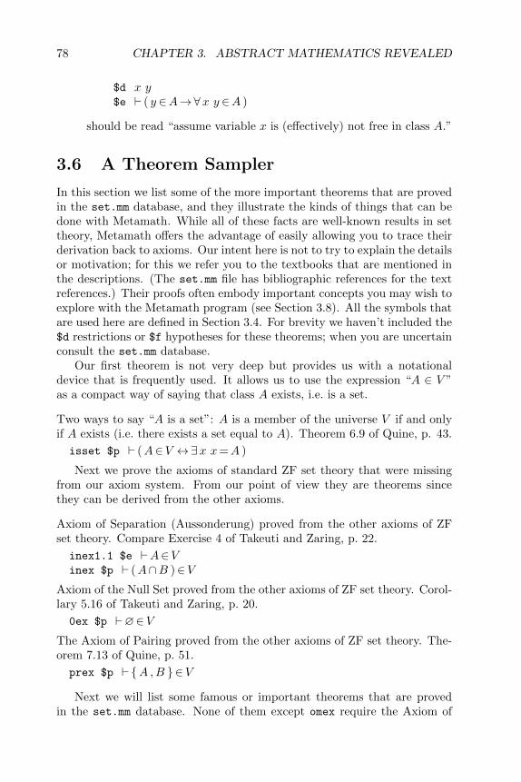
78 CHAPTER 3. ABSTRACT MATHEMATICS REVEALED
$d x y$e ` ( y ∈A→∀x y ∈A )
should be read “assume variable x is (effectively) not free in class A.”
3.6 A Theorem Sampler
In this section we list some of the more important theorems that are provedin the set.mm database, and they illustrate the kinds of things that can bedone with Metamath. While all of these facts are well-known results in settheory, Metamath offers the advantage of easily allowing you to trace theirderivation back to axioms. Our intent here is not to try to explain the detailsor motivation; for this we refer you to the textbooks that are mentioned inthe descriptions. (The set.mm file has bibliographic references for the textreferences.) Their proofs often embody important concepts you may wish toexplore with the Metamath program (see Section 3.8). All the symbols thatare used here are defined in Section 3.4. For brevity we haven’t included the$d restrictions or $f hypotheses for these theorems; when you are uncertainconsult the set.mm database.
Our first theorem is not very deep but provides us with a notationaldevice that is frequently used. It allows us to use the expression “A ∈ V ”as a compact way of saying that class A exists, i.e. is a set.
Two ways to say “A is a set”: A is a member of the universe V if and onlyif A exists (i.e. there exists a set equal to A). Theorem 6.9 of Quine, p. 43.
isset $p ` (A∈V ↔∃x x=A )
Next we prove the axioms of standard ZF set theory that were missingfrom our axiom system. From our point of view they are theorems sincethey can be derived from the other axioms.
Axiom of Separation (Aussonderung) proved from the other axioms of ZFset theory. Compare Exercise 4 of Takeuti and Zaring, p. 22.
inex1.1 $e `A∈Vinex $p ` (A∩B )∈V
Axiom of the Null Set proved from the other axioms of ZF set theory. Corol-lary 5.16 of Takeuti and Zaring, p. 20.
0ex $p `∅∈VThe Axiom of Pairing proved from the other axioms of ZF set theory. The-orem 7.13 of Quine, p. 51.
prex $p ` {A ,B }∈V
Next we will list some famous or important theorems that are provedin the set.mm database. None of them except omex require the Axiom of

3.6. A THEOREM SAMPLER 79
Infinity, as you can verify with the show trace_back Metamath command.
The resolution of Russell’s paradox. There exists no set containing the setof all sets which are not members of themselves. Proposition 4.14 of Takeutiand Zaring, p. 14.
ru $p `¬∃x x= { y | ¬ y ∈ y }Cantor’s theorem. No set can be mapped onto its power set. CompareTheorem 6B(b) of Enderton, p. 132.
canth.1 $e `A∈Vcanth $p `¬F :A −→onto P A
The Burali-Forti paradox. No set contains all ordinal numbers. Enderton,p. 194. (Burali-Forti was one person, not two.)
onprc $p `¬On∈VPeano’s postulates for arithmetic. Proposition 7.30 of Takeuti and Zaring,pp. 42–43. The objects being described are the members of ω i.e. the naturalnumbers 0, 1, 2,. . . . The successor operation suc means “plus one.” peano1
says that 0 (which is defined as the empty set) is a natural number. peano2says that if A is a natural number, so is A + 1. peano3 says that 0 is notthe successor of any natural number. peano4 says that two natural numbersare equal if and only if their successors are equal. peano5 is essentially thesame as mathematical induction.
peano1 $p `∅∈ω
peano2 $p ` (A∈ω→ sucA∈ω )
peano3 $p ` (A∈ω→¬ sucA=∅ )
peano4 $p ` ( (A∈ω ∧B ∈ω )→ ( sucA= sucB↔A=B ) )
peano5 $p ` ( (∅∈A∧∀x∈ω (x∈A→ sucx∈A ) )→ω⊆A )
Finite Induction (mathematical induction). The first hypothesis is the basisand the second is the induction hypothesis. Theorem Schema 22 of Suppes,p. 136.
findes.1 $e ` [∅ / x ]ϕfindes.2 $e ` (x∈ω→ (ϕ→ [ sucx /x ]ϕ ) )findes $p ` (x∈ω→ϕ )
Transfinite Induction with explicit substitution. The first hypothesis is thebasis, the second is the induction hypothesis for successors, and the third isthe induction hypothesis for limit ordinals. Theorem Schema 4 of Suppes,p. 197.
tfindes.1 $e ` [∅ / x ]ϕtfindes.2 $e ` (x∈On→ (ϕ→ [ sucx /x ]ϕ ) )tfindes.3 $e ` ( Lim y→ (∀x∈ y ϕ→ [ y / x ]ϕ ) )

80 CHAPTER 3. ABSTRACT MATHEMATICS REVEALED
tfindes $p ` (x∈On→ϕ )
Principle of Transfinite Recursion. Theorem 7.41 of Takeuti and Zaring,p. 47. Transfinite recursion is the key theorem that allows arithmetic ofordinals to be rigorously defined, and has many other important uses aswell. Hypotheses tfr.1 and tfr.2 specify a certain (proper) class F . Thecomplicated definition of F is not important in itself; what is important isthat there be such an F with the required properties, and we show this bydisplaying F explicitly. tfr1 states that F is a function whose domain isthe set of ordinal numbers. tfr2 states that any value of F is completelydetermined by its previous values and the values of an auxiliary function,G. tfr3 states that F is unique, i.e. it is the only function that satisfiestfr1 and tfr2. Note that f is an individual variable like x and y; it is justa mnemonic to remind us that A is a collection of functions.
tfr.1 $e `A= { f | ∃x∈On ( f Fnx∧∀ y ∈x ( f ‘ y ) = (G ‘ ( f � y ) ) ) }tfr.2 $e `F =
⋃A
tfr1 $p `F Fn Ontfr2 $p ` ( z ∈On→ (F ‘ z ) = (G ‘ (F � z ) ) )tfr3 $p ` ( (B Fn On∧∀x∈On (B ‘x ) = (G ‘ (B �x ) ) )→B=F )
The existence of omega (the class of natural numbers). Axiom 7 of Takeutiand Zaring, p. 43. (This is the only theorem in this section requiring theAxiom of Infinity.)
omex $p `ω ∈V
3.7 Axioms for Real and Complex Numbers
This section presents the axioms for real and complex numbers. Analysistextbooks implicitly or explicity use these axioms or their equivalents areused as their starting point. In the database set.mm, we define real andcomplex numbers as (rather complicated) specific sets and derive these ax-ioms as theorems from the axioms of ZF set theory, using a method calledDedekind cuts. We omit the details of this construction, which you can fol-low if you wish using the set.mm database in conjunction with the textbooksreferenced therein. The construction is actually unimportant other than toshow that sets exist that satisfy the axioms, and thus that the axioms areconsistent if ZF set theory is consistent. When working with real numbersyou can think of them as being the actual sets resulting from the construc-tion (for definiteness), or you can think of them as otherwise unspecifiedsets that happen to satisfy the axioms.
For the axioms we are given (or postulate) 8 classes: C (the set of complexnumbers), R (the set of real numbers, a subset of C), 0 (zero), 1 (one), i(square root of −1), + (plus), · (times), and < (less than). Subtractionand division are defined terms and are not part of the axioms; for theirdefinitions see set.mm.
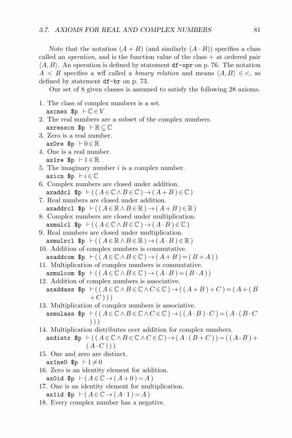
3.7. AXIOMS FOR REAL AND COMPLEX NUMBERS 81
Note that the notation (A + B) (and similarly (A · B)) specifies a classcalled an operation, and is the function value of the class + at ordered pair〈A,B〉. An operation is defined by statement df-opr on p. 76. The notationA < B specifies a wff called a binary relation and means 〈A,B〉 ∈<, asdefined by statement df-br on p. 73.
Our set of 8 given classes is assumed to satisfy the following 28 axioms.
1. The class of complex numbers is a set.axcnex $p `C∈V
2. The real numbers are a subset of the complex numbers.axresscn $p `R⊆C
3. Zero is a real number.ax0re $p ` 0∈R
4. One is a real number.ax1re $p ` 1∈R
5. The imaginary number i is a complex number.axicn $p ` i∈C
6. Complex numbers are closed under addition.axaddcl $p ` ( (A∈C∧B ∈C )→ (A+B )∈C )
7. Real numbers are closed under addition.axaddrcl $p ` ( (A∈R∧B ∈R )→ (A+B )∈R )
8. Complex numbers are closed under multiplication.axmulcl $p ` ( (A∈C∧B ∈C )→ (A ·B )∈C )
9. Real numbers are closed under multiplication.axmulrcl $p ` ( (A∈R∧B ∈R )→ (A ·B )∈R )
10. Addition of complex numbers is commutative.axaddcom $p ` ( (A∈C∧B ∈C )→ (A+B ) = (B+A ) )
11. Multiplication of complex numbers is commutative.axmulcom $p ` ( (A∈C∧B ∈C )→ (A ·B ) = (B ·A ) )
12. Addition of complex numbers is associative.axaddass $p ` ( (A∈C∧B ∈C∧C ∈C )→ ( (A+B ) +C ) = (A+ (B
+C ) ) )13. Multiplication of complex numbers is associative.axmulass $p ` ( (A∈C∧B ∈C∧C ∈C )→ ( (A ·B ) ·C ) = (A · (B ·C
) ) )14. Multiplication distributes over addition for complex numbers.axdistr $p ` ( (A∈C∧B ∈C∧C ∈C )→ (A · (B+C ) ) = ( (A ·B ) +
(A ·C ) ) )15. One and zero are distinct.ax1ne0 $p ` 1 6= 0
16. Zero is an identity element for addition.ax0id $p ` (A∈C→ (A+ 0 ) =A )
17. One is an identity element for multiplication.ax1id $p ` (A∈C→ (A · 1 ) =A )
18. Every complex number has a negative.

82 CHAPTER 3. ABSTRACT MATHEMATICS REVEALED
axnegex $p ` (A∈C→∃x∈C (A+x ) = 0 )19. Every nonzero complex number has a reciprocal.axrecex $p ` (A∈C→ (A 6= 0→∃x∈C (A ·x ) = 1 ) )
20. Every real number has a negative.axrnegex $p ` (A∈R→∃x∈R (A+x ) = 0 )
21. Every nonzero real number has a reciprocal.axrrecex $p ` (A∈R→ (A 6= 0→∃x∈R (A ·x ) = 1 ) )
22. The square of i equals −1 (expressed as i-squared plus 1 is 0).axi2m1 $p ` ( ( i · i ) + 1 ) = 0
23. Ordering on reals satisfies strict trichotomy.axlttri $p ` ( (A∈R∧B ∈R )→ (A<B↔¬ (A=B ∨B<A ) ) )
24. Ordering on reals is transitive.axlttrn $p ` ( (A∈R∧B ∈R∧C ∈R )→ ( (A<B ∧B<C )→A<C )
)25. Ordering on reals is preserved after addition to both sides.axltadd $p ` ( (A∈R∧B ∈R∧C ∈R )→ (A<B→ (C +A )< (C +
B ) ) )26. The product of two positive reals is positive.axmulgt0 $p ` ( (A∈R∧B ∈R )→ ( ( 0<A∧ 0<B )→ 0< (A ·B ) ) )
27. A complex number can be expressed in terms of two reals.axcnre $p ` (A∈C→∃x∈R ∃ y ∈RA= (x+ ( y · i ) ) )
28. A non-empty, bounded-above set of reals has a supremum.axsup $p ` ( (A⊆R∧A 6=∅∧∃x∈R ∀ y ∈A y<x )→∃x∈R (∀ y ∈A
¬x<y ∧∀ y ∈R ( y <x→∃ z ∈A y<z ) ) )
This completes the set of axioms for real and complex numbers. Youmay wish to look at how subtraction, division, and decimal numbers aredefined in set.mm, and for fun look at the proof of 2+2 = 4 (theorem 2p2e4
in set.mm).In set.mm we define the non-negative integers N, the integers Z, and the
rationals Q as subsets of R. This leads the nice inclusion N ⊆ Z ⊆ Q ⊆R ⊆ C, giving us a uniform framework in which, for example, a propertysuch as commutativity of complex number addition automatically appliesto integers. The natural numbers N are different from the set ω we definedearlier, but both satisfy Peano’s postulates.
Complex Number Axioms in Analysis Texts
Most analysis texts construct complex numbers as ordered pairs of reals,leading to construction-dependent properties that satisfy these axioms butare not stated in their pure form. (This is also done in set.mm but ouraxioms are extracted from that construction.) Other texts will simply statethat R is a “complete ordered subfield of C,” leading to redundant axiomswhen this phrase is completely expanded out. In fact I have not seen a textwith the axioms in the explicit form above. It is possible that one or more

3.8. EXPLORING THE SET THEORY DATABASE 83
of the axioms above are redundant or could be made weaker; if you discoveran improvement, please let me know, and I will properly acknowledge yourcontribution. Update (Feb. 2005): The third axiom, “0 is a real number,”is redundant; see the http://metamath.org web site for details.
3.8 Exploring the Set Theory Database
At this point you may wish to study the set.mm file in more detail. Payparticular attention to the assumptions needed to define wffs (which are notincluded above), the variable types ($f statements), and the definitions thatare introduced. Start with some simple theorems in propositional calculus,making sure you understand in detail each step of a proof. Once you get pastthe first few proofs and become familiar with the Metamath language, anypart of the set.mm database will be as easy to follow, step by step, as anyother part—you won’t have to undergo a “quantum leap” in mathematicalsophistication to be able to follow a deep proof in set theory.
Next, you may want to explore how concepts such as natural numbersare defined and described. This is probably best done in conjunction withstandard set theory textbooks, which can help give you a higher-level un-derstanding. The set.mm database provides references that will get youstarted. From there, you will be on your way towards a very deep, rigorousunderstanding of abstract mathematics.
The Metamath program can help you peruse a Metamath database,whether you are trying to figure out how a certain step follows in a proofor just have a general curiosity. We will go through some examples of thecommands, using the set.mm database provided with the Metamath soft-ware. These should help get you started. See Chapter 5 for a more detaileddescription of the commands. Note that we have included the full spellingof all commands to prevent ambiguity with future commands. In practiceyou may type just the characters needed to specify each command keywordunambiguously, often just one or two characters per keyword, and you don’tneed to type them in upper case.
First run the Metamath program as described earlier. You should seethe MM> prompt. Read in the set.mm file:
MM> read set.mm
Reading source file "set.mm"...
73689 lines (3543983 characters) were read from "set.mm".
The source has 21443 statements; 417 are $a and 5989 are $p.
No errors were found. However, proofs were not checked.
Type VERIFY PROOF * if you want to check them.
Let’s check the database integrity. This may take a minute or two to runif your computer is slow.

84 CHAPTER 3. ABSTRACT MATHEMATICS REVEALED
MM> verify proof *
0 10% 20% 30% 40% 50% 60% 70% 80% 90% 100%
..................................................
All proofs in the database were verified in 2.84 s.
No errors were reported, so every proof is correct.You need to know the names (labels) of theorems before you can look at
them. Often just examining the database file(s) with a text editor is the bestapproach. In set.mm there are many detailed comments, especially near thebeginning, that can help guide you. The search command in the Metamathprogram is also handy. The comments qualifier will list the statements whoseassociated comment (the one immediately before it) contain a string you giveit. For example, if you are studying Enderton’s Elements of Set Theory [16]you may want to see the references to it in the database. The search stringenderton is not case sensitive. (This will not show you all the databasetheorems that are in Enderton’s book because there is usually only onecitation for a given theorem, which may appear in several textbooks.)
MM> search * "enderton" / comments
3332 df-ral $a "...niversal quantification. Enderton, p. 22."
3333 df-rex $a "...stential quantification. Enderton, p. 22."
4828 df-tp $a "...of classes. Definition of Enderton, p. 19."
5200 ssuniss $p "...nd union. Exercise 5 of Enderton, p. 26."
5217 opeluu $p "...air belongs. Lemma 3D of Enderton, p. 41."
(etc.)
Or you may want to see what theorems have something to do with con-junction (logical and). The quotes around the search string are optionalwhen there’s no ambiguity.
MM> search * conjunction / comments
634 wa $a "...wff definition to include conjunction (’and’)."
636 df-an $a "Define conjunction (’and’)."
654 iman $p "Express implication in terms of conjunction."
655 annim $p "Express conjunction in terms of implication."
687 pm3.2 $p "... antecedents with conjunction. Theorem *..."
751 anor $p "Conjunction in terms of disjunction (de Morg..."
(etc.)
Now we will start to look at some details. Let’s look at the first axiomof propositional calculus.
MM> show statement ax-1/full
MM> sh st ax-1/full

3.8. EXPLORING THE SET THEORY DATABASE 85
Statement 19 is located on line 881 of the file "set.mm".
"Axiom _Simp_. Axiom A1 of [Margaris] p. 49. One of the 3
axioms of propositional calculus. The 3 axioms are also
...
19 ax-1 $a |- ( ph -> ( ps -> ph ) ) $.
Its mandatory hypotheses in RPN order are:
wph $f wff ph $.
wps $f wff ps $.
The statement and its hypotheses require the variables: ph
ps
The variables it contains are: ph ps
Compare this to ax-1 on p. 64. You can see that the symbol ph isthe ascii notation for ϕ, etc. To see the mathematical symbols for anyexpression you may typeset it in LATEX (type help tex for instructions) or,easier, just use a text editor to look at the comments where symbols are firstintroduced in set.mm. The hypotheses wph and wps required by ax-1 meanthat variables ph and ps must be wffs.
Next we’ll pick a simple theorem of propositional calculus, the Principleof Identity, which is proved directly from the axioms. We’ll look at thestatement then its proof.
MM> show statement id1/full
Statement 36 is located on line 968 of the file "set.mm".
"Principle of identity. Theorem *2.08 of Whitehead and
Russell. This version is proved directly from the axioms
for demonstration purposes."
id1 $p |- ( ph -> ph ) $= ... $.
Its mandatory hypotheses in RPN order are:
wph $f wff ph $.
Its optional hypotheses are: wps wch wth wet
The statement and its hypotheses require the variables: ph
These additional variables are allowed in its proof: ps ch
th et
The variables it contains are: ph
The optional variables ps, ch, etc. are available for use in a proof ofthis statement if we wish, and were we to do so we would make use ofoptional hypotheses wps, wch, etc. (See Section 4.2.5 for the meaning of“optional hypothesis.”) The reason these show up in the statement displayis that statement id1 happens to be in their scope (see Section 4.2.8 forthe definition of “scope”), but in fact in propositional calculus we will nevermake use of optional hypotheses or variables. This becomes important afterquantifiers are introduced, where “dummy” variables are often needed in themiddle of a proof.

86 CHAPTER 3. ABSTRACT MATHEMATICS REVEALED
Let’s look at the proof of statement id1. We’ll suppress the “non-essential” steps that construct the wffs.
MM> show proof id1/essential/lemmon/renumber
1 ax-2 $a |- ( ( ph -> ( ( ph -> ph ) -> ph ) ) ->
( ( ph -> ( ph -> ph ) ) -> ( ph -> ph )
) )
2 ax-1 $a |- ( ph -> ( ( ph -> ph ) -> ph ) )
3 1,2 ax-mp $a |- ( ( ph -> ( ph -> ph ) ) -> ( ph -> ph
) )
4 ax-1 $a |- ( ph -> ( ph -> ph ) )
5 3,4 ax-mp $a |- ( ph -> ph )
If you have read Section 2.3, you’ll know how to interpret this proof.Step 2, for example, is an application of axiom ax-1. This proof is identicalto the one in Hamilton’s Logic for Mathematicians [19, p. 32].
You may want to look at what substitutions are made into ax-1 to arriveat step 2. The command to do this needs to know the “real” step number,so we’ll display the proof again without the renumber qualifier.
MM> show proof id1/lemmon/essential
18 ax-2 $a |- ( ( ph -> ( ( ph -> ph ) -> ph ) ) ->
( ( ph -> ( ph -> ph ) ) -> ( ph -> ph )
) )
21 ax-1 $a |- ( ph -> ( ( ph -> ph ) -> ph ) )
22 18,21 ax-mp $a |- ( ( ph -> ( ph -> ph ) ) -> ( ph -> ph
) )
25 ax-1 $a |- ( ph -> ( ph -> ph ) )
26 22,25 ax-mp $a |- ( ph -> ph )
The “real” step number is 21. Let’s look at its details.
MM> show proof id1 /detailed_step 21
Proof step 21: min=ax-1 $a |- ( ph -> ( ( ph -> ph ) -> ph )
)
This step assigns source "ax-1" ($a) to target "min" ($e).
The source assertion requires the hypotheses "wph" ($f, step
19) and "wps" ($f, step 20). The parent assertion of the
target hypothesis is "ax-mp" ($a, step 22).
The source assertion before substitution was:
ax-1 $a |- ( ph -> ( ps -> ph ) )
The following substitutions were made to the source
assertion:
Variable Substituted with
ph ph
ps ( ph -> ph )

3.8. EXPLORING THE SET THEORY DATABASE 87
The target hypothesis before substitution was:
min $e |- ph
The following substitution was made to the target hypothesis:
Variable Substituted with
ph ( ph -> ( ( ph -> ph ) -> ph ) )
This shows the substitutions made to the variables in ax-1. Referencesare made to steps 19 and 20 which are not shown in our proof display. Tosee these steps, you can display the proof without the essential qualifier.
Let’s look at a slightly more advanced proof of propositional calculus.Note that /\ is the symbol for ∧ (logical and, also called conjunction).
MM> show statement prth/full
Statement 1521 is located on line 4730 of the file "set.mm".
"Theorem *3.47 of Whitehead and Russell, called ’praeclarum
theorema’ by Leibniz."
prth $p |- ( ( ( ph -> ps ) /\ ( ch -> th ) ) -> ( ( ph /\
ch ) -> ( ps /\ th ) ) ) $= ... $.
Its mandatory hypotheses in RPN order are:
wph $f wff ph $.
wps $f wff ps $.
wch $f wff ch $.
wth $f wff th $.
Its optional hypotheses are: wet
The statement and its hypotheses require the variables: ph
ps ch th
These additional variables are allowed in its proof: et
The variables it contains are: ph ps ch th
MM> show proof prth/essential/lemmon/renumber
1 pm3.2 $p |- ( ps -> ( th -> ( ps /\ th ) ) )
2 1 syl3dt $p |- ( ps -> ( ( ch -> th ) -> ( ch -> ( ps
/\ th ) ) ) )
3 2 syl3 $p |- ( ( ph -> ps ) -> ( ph -> ( ( ch -> th
) -> ( ch -> ( ps /\ th ) ) ) ) )
4 3 com23 $p |- ( ( ph -> ps ) -> ( ( ch -> th ) -> (
ph -> ( ch -> ( ps /\ th ) ) ) ) )
5 4 impa $p |- ( ( ( ph -> ps ) /\ ( ch -> th ) ) ->
( ph -> ( ch -> ( ps /\ th ) ) ) )
6 impexp $p |- ( ( ( ph /\ ch ) -> ( ps /\ th ) ) <->
( ph -> ( ch -> ( ps /\ th ) ) ) )
7 5,6 sylibr $p |- ( ( ( ph -> ps ) /\ ( ch -> th ) ) ->
( ( ph /\ ch ) -> ( ps /\ th ) ) )
There are references to a lot of unfamiliar statements. To see what theyare, you may type the following:

88 CHAPTER 3. ABSTRACT MATHEMATICS REVEALED
MM> show proof prth/statement_summary/essential
Summary of statements used in the proof of "prth":
Statement "syl3" is located on line 355 of the file "set.mm".
"Inference adding common antecedents in an implication."
syl3.1 $e |- ( ph -> ps ) $.
syl3 $p |- ( ( ch -> ph ) -> ( ch -> ps ) ) $= ... $.
Statement "syl3dt" is located on line 438 of the file
"set.mm".
"Deduction adding nested antecedents."
syl3dt.1 $e |- ( ph -> ( ps -> ch ) ) $.
syl3dt $p |- ( ph -> ( ( th -> ps ) -> ( th -> ch ) ) ) $=
... $.
(etc.)
Of course you can look at each of these statements and their proofs, andso on, back to the axioms of propositional calculus if you wish.
The search command is useful for finding statements when you know allor part of their contents. The following example finds all statements con-taining ph -> ps followed by ch -> th. The $* is a wildcard that matchesanything; the $ before the * prevents conflicts with math symbol tokennames. The * after SEARCH is also a wildcard that in this case means “matchany label.”
MM> SEARCH * "ph -> ps $* ch -> th"
1521 prth $p |- ( ( ( ph -> ps ) /\ ( ch -> th ) ) -> ( ( ph
/\ ch ) -> ( ps /\ th ) ) )
1522 pm3.48 $p |- ( ( ( ph -> ps ) /\ ( ch -> th ) ) -> ( (
ph \/ ch ) -> ( ps \/ th ) ) )
1739 elimant $p |- ( ( ( ph -> ps ) /\ ( ( ps -> ch ) -> ( ph
-> th ) ) ) -> ( ph -> ( ch -> th ) ) )
Three statements, prth, pm3.48, and elimant, were found to match.To see what axioms and definitions prth ultimately depends on for its
proof, you can have the program backtrack through the hierarchy of theo-rems and definitions.
MM> show trace_back prth /essential/axioms
Statement "prth" assumes the following axioms ($a
statements):
ax-1 ax-2 ax-3 ax-mp df-bi df-an
Note that the 3 axioms of propositional calculus and the modus ponensrule are needed (as expected); in addition, there are a couple of definitions
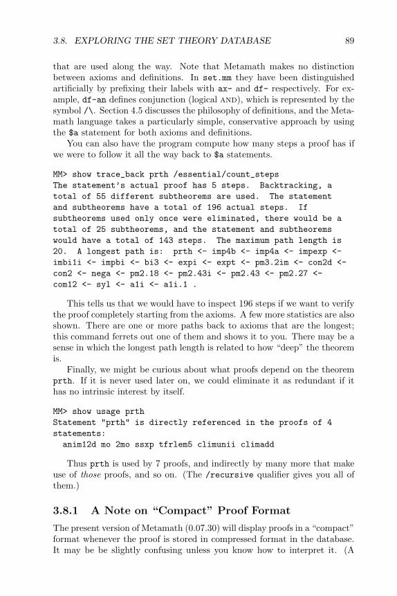
3.8. EXPLORING THE SET THEORY DATABASE 89
that are used along the way. Note that Metamath makes no distinctionbetween axioms and definitions. In set.mm they have been distinguishedartificially by prefixing their labels with ax- and df- respectively. For ex-ample, df-an defines conjunction (logical and), which is represented by thesymbol /\. Section 4.5 discusses the philosophy of definitions, and the Meta-math language takes a particularly simple, conservative approach by usingthe $a statement for both axioms and definitions.
You can also have the program compute how many steps a proof has ifwe were to follow it all the way back to $a statements.
MM> show trace_back prth /essential/count_steps
The statement’s actual proof has 5 steps. Backtracking, a
total of 55 different subtheorems are used. The statement
and subtheorems have a total of 196 actual steps. If
subtheorems used only once were eliminated, there would be a
total of 25 subtheorems, and the statement and subtheorems
would have a total of 143 steps. The maximum path length is
20. A longest path is: prth <- imp4b <- imp4a <- impexp <-
imbi1i <- impbi <- bi3 <- expi <- expt <- pm3.2im <- con2d <-
con2 <- nega <- pm2.18 <- pm2.43i <- pm2.43 <- pm2.27 <-
com12 <- syl <- a1i <- a1i.1 .
This tells us that we would have to inspect 196 steps if we want to verifythe proof completely starting from the axioms. A few more statistics are alsoshown. There are one or more paths back to axioms that are the longest;this command ferrets out one of them and shows it to you. There may be asense in which the longest path length is related to how “deep” the theoremis.
Finally, we might be curious about what proofs depend on the theoremprth. If it is never used later on, we could eliminate it as redundant if ithas no intrinsic interest by itself.
MM> show usage prth
Statement "prth" is directly referenced in the proofs of 4
statements:
anim12d mo 2mo ssxp tfrlem5 climunii climadd
Thus prth is used by 7 proofs, and indirectly by many more that makeuse of those proofs, and so on. (The /recursive qualifier gives you all ofthem.)
3.8.1 A Note on “Compact” Proof Format
The present version of Metamath (0.07.30) will display proofs in a “compact”format whenever the proof is stored in compressed format in the database.It may be be slightly confusing unless you know how to interpret it. (A

90 CHAPTER 3. ABSTRACT MATHEMATICS REVEALED
future version may eliminate this format from displays.) For example, ifyou display the complete proof of theorem id1 it will start off as follows:
MM> show proof id1 /lemmon/all
1 wph $f wff ph
2 wph $f wff ph
3 wph $f wff ph
4 2,3 wi @1: $a wff ( ph -> ph )
5 1,4 wi @2: $a wff ( ph -> ( ph -> ph ) )
6 @1 $a wff ( ph -> ph )
etc.
Step 4 has a “local label,” @1, assigned to it. Later on, at step 6, thelabel @1 is referenced instead of displaying the explicit proof for that step.This technique takes advantage of the fact that steps in a proof often repeat,especially during the construction of wffs. The compact format reduces thenumber of steps in the proof display and may actually be preferred by somepeople, which is one reason that it is still displayed by the program.
If you want to see the normal format with the “true” step numbers, youcan use the following workaround:
MM> save proof id1 /normal
The proof of "id1" has been reformatted and saved internally.
Remember to use WRITE SOURCE to save it permanently.
MM> show proof id1 /lemmon/all
1 wph $f wff ph
2 wph $f wff ph
3 wph $f wff ph
4 2,3 wi $a wff ( ph -> ph )
5 1,4 wi $a wff ( ph -> ( ph -> ph ) )
6 wph $f wff ph
7 wph $f wff ph
8 6,7 wi $a wff ( ph -> ph )
etc.
Note that the original 6 steps are now 8 steps. However, the format isnow the same as that described in Chapter 2.

Chapter 4
The Metamath Language
Thus mathematics may be defined as the subject in which wenever know what we are talking about, nor whether what we aresaying is true.
Bertrand Russell1
Probably the most striking feature of the Metamath language is its al-most complete absence of hard-wired syntax. Metamath does not under-stand any mathematics or logic other than that needed to construct finitesequences of symbols according to a small set of simple, built-in rules. Theonly rule it uses in a proof is the substitution of an expression (symbolsequence) for a variable, subject to a simple constraint to prevent bound-variable clashes. The primitive notions built into Metamath involve thesimple manipulation of finite objects (symbols) that we as humans can eas-ily visualize and that computers can easily deal with. They seem to bejust about the simplest notions possible that are required to do standardmathematics.
This chapter serves as a reference manual for the Metamath language. Itcovers the tedious technical details of the language, some of which you maywish to skim in a first reading. On the other hand, you should pay closeattention to the defined terms in boldface; they have precise meanings thatare important to keep in mind for later understanding. It may be best to firstbecome familiar with the examples in Chapter 2 to gain some motivationfor the language.
If you have some knowledge of set theory, you may wish to study thischapter in conjunction with the formal set-theoretical description of theMetamath language in Appendix C.
We will use the name “Metamath” to mean either the Metamath com-puter language or the Metamath software associated with the computer
1[52, p. 84]
91

92 CHAPTER 4. THE METAMATH LANGUAGE
language. We will not distinguish these two when the context is clear.The next section contains the complete specification of the Metamath
language.2 It serves as an authoritative reference and presents the syntaxin enough detail to write a parser and proof verifier. The specification isterse and it is probably hard to learn the language directly from it, but weinclude it here for those impatient people who prefer to see everything upfront before looking at verbose expository material. Later sections explainthis material and provide examples. We will repeat the definitions in thosesections, and you may skip the next section at first reading and proceed toSection 4.2 (p. 96). You may want to come back to it to clarify any finepoints.
4.1 Specification of the Metamath Language
Sometimes one has to say difficult things, but one ought to saythem as simply as one knows how.
G. H. Hardy3
4.1.1 Preliminaries
A Metamath database is built up from a top-level source file together withany source files that are brought in through file inclusion commands (seebelow). The only characters that are allowed to appear in a Metamathsource file are the 94 printable characters on standard ascii keyboards,which are digits, upper and lower case letters, and the following 32 specialcharacters
‘ ~ ! @ # $ % ^ & * ( ) - _ = +
[ ] { } ; : ’ " , . < > / ? \ |
plus the following non-printable (white space) characters: space, tab, car-riage return, line feed, and form feed. We will use typewriter font to displaythe printable characters.
A Metamath database consists of a sequence of three kinds of tokensseparated by white space (which is any sequence of one or more whitespace characters). The set of keyword tokens is ${, $}, $c, $v, $f, $e,$d, $a, $p, $., $=, $(, $), $[, and $]. The last four are called auxiliary
2The current version of the Metamath program (0.07.30) implements an older speci-fication with a slightly more general syntax than described here. Among the differences:missing white space around keyword tokens is sometimes tolerated, and a variable maybe used before its type is specified by a $f statement (this “feature” should never beused in practice). A future version of the program is expected to conform to the currentspecification.
3As quoted in [14], p. 273

4.1. SPECIFICATION OF THE METAMATH LANGUAGE 93
or preprocessing keywords. A label token consists of any combination ofletters, digits, and the characters hyphen, underscore, and period. A mathsymbol token may consist of any combination of the 93 printable standardascii characters other than $ . All tokens are case-sensitive.
4.1.2 Preprocessing
$( begins a comment and $) ends a comment. Comments may containany of the 94 printable characters and white space, except they may notcontain the 2-character sequences $( or $). Comments are ignored (treatedlike white space) for the purpose of parsing.
Two special characters inside comments, ‘ and ~, control the typesettingof comments and are discussed on p. 119. They may be ignored for thepurpose of parsing.
A file inclusion command consists of $[ followed by a file name fol-lowed by $]. The file name may not contain a $ or white space. The filemust exist. The case-sensitivity of its name follows the conventions of theoperating system. The contents of the file replace the inclusion command.Included files may include other files. Only the first reference to a given fileis included; any later references to the same file (whether in the top-levelfile or in included files) cause the inclusion command to be ignored (treatedlike white space). A file self-reference is ignored, as is any reference to thetop-level file.
Like all tokens, the $(, $), $[, and $] keywords must be surrounded bywhite space.
4.1.3 Basic Syntax
After preprocessing, a database will consist of a sequence of statements.It may contain only the statement types defined below. These are the scop-ing statements ${ and $}, along with the $c, $v, $f, $e, $d, $a, and $p
statements.A scoping statement consists only of its keyword, ${ or $}. ${ begins
a block and a matching $} ends the block. Every ${ must have a matching$}. Defining it recursively, we say a block contains a sequence of zero ormore tokens other than ${ and $} and possibly other blocks. There is anoutermost block not bracketed by ${ $}; the end of the outermost blockis the end of the database.
A $v or $c statement consists of the keyword token $v or $c respec-tively, followed by one or more math symbols, followed by $. . These state-ments declare the math symbols to be variables or constants respectively.The same math symbol may not occur twice in a given $v or $c statement.
A math symbol becomes active when declared and stays active until theend of the block in which it is declared. A variable may not be declared asecond time while it is active, but it may be declared again (as a variable, but

94 CHAPTER 4. THE METAMATH LANGUAGE
not as a constant) after it becomes inactive. A constant must be declaredin the outermost block and may not be declared a second time.4
A $f statement consists of a label, followed by $f, followed by an activeconstant, followed by an active variable, followed by $. . A $e statementconsists of a label, followed by $e, followed by an active constant, followedzero or more active math symbols, followed by $. . A hypothesis is a $f
or $e statement.A simple $d statement consists of $d, followed by two different active
variables, followed by $. . A compound $d statement consists of $d,followed by three or more variables (all different), followed by $. . Theorder of the variables in a $d statement is unimportant. A compound $d
statement is equivalent to a set of simple $d statements, one for each possiblepair of variables occurring in the compound $d statement. Henceforth in thisspecification we shall assume all $d statements are simple. A $d statementis also called a disjoint (or distinct) variable restriction.
A $a statement consists of a label, followed by $a, followed by an activeconstant, followed by zero or more active math symbols, followed by $. . A$p statement consists of a label, followed by $p, followed by an activeconstant, followed by zero or more active math symbols, followed by $=,followed by a sequence of labels, followed by $. . An assertion is a $a or$p statement.
A $f, $e, or $d statement is active from the place it occurs until theend of the block it occurs in. A $a or $p statement is active from the placeit occurs through the end of the database.
There may not be two active $f statements containing the same vari-able. Each variable in a $e, $a, or $p statement must exist in an active $f
statement.5
Each label token must be unique.No label token may match any math symbol token.6
The set of mandatory variables associated with an assertion is the setof (zero or more) variables in the assertion and in any active $e statements.The (possibly empty) set of mandatory hypotheses is the set of all active$f statements containing mandatory variables, together with all active $e
statements.The set of mandatory $d statements associated with an assertion are
those active $d statements whose variables are both among the assertion’smandatory variables.
4The rules for redeclaration may become more general in the future; see footnote onp. 114.
5This requirement can greatly simplify the unification algorithm (substitution calcu-lation) required by proof verification.
6(Added June 24, 2006) This restriction did not exist in earlier versions of this specifi-cation. While not theoretically necessary, it is imposed to make it easier to write certainparsers.

4.1. SPECIFICATION OF THE METAMATH LANGUAGE 95
4.1.4 Proof Verification
The sequence of labels between the $= and $. tokens in a $p statement isa proof. Each label in a proof must be the label of an active statementother than the $p statement itself; thus a label must refer either to an activehypothesis of the $p statement or to an earlier assertion.
An expression is a sequence of math symbols. A substitution mapassociates a set of variables with a set of expressions. It is acceptable fora variable to be mapped to an expression containing it. A substitutionis the simultaneous replacement of all variables in one or more expressionswith the expressions that the variables map to.
A proof is scanned in order of its label sequence. If the label refersto an active hypothesis, the expression in the hypothesis is pushed onto astack. If the label refers to an assertion, a (unique) substitution must existthat, when made to the mandatory hypotheses of the referenced assertion,causes them to match the topmost (i.e. most recent) entries of the stack, inorder of occurrence of the mandatory hypotheses, with the topmost stackentry matching the last mandatory hypothesis of the referenced assertion.As many stack entries as there are mandatory hypotheses are then poppedfrom the stack. The same substitution is made to the referenced assertion,and the result is pushed onto the stack. After the last label in the proof isprocessed, the stack must have a single entry that matches the expressionin the $p statement containing the proof.
A proof may contain a ? in place of a label to indicate an unknownstep (Section 4.4.5). A proof verifier may ignore any proof containing ? butshould warn the user that the proof is incomplete.
A compressed proof is an alternate proof notation described in Appen-dix B; also see references to “compressed proof” in the Index. Compressedproofs are a Metamath language extension which a complete proof verifiershould be able to parse and verify.
Verifying Disjoint Variable Restrictions
Each substitution made in a proof must be checked to verify that any disjointvariable restrictions are satisfied, as follows.
If two variables replaced by a substitution exist in a mandatory $d state-ment of the assertion referenced, the two expressions resulting from thesubstitution must meet satisfy the following conditions. First, the two ex-pressions must have no variables in common. Second, each possible pair ofvariables, one from each expression, must exist in an active $d statement ofthe $p statement containing the proof.
This ends the specification of the Metamath language.
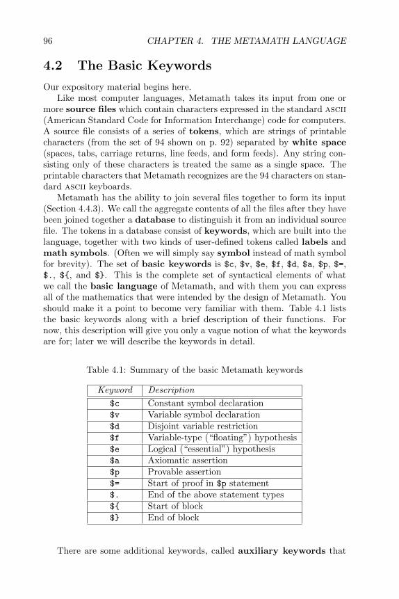
96 CHAPTER 4. THE METAMATH LANGUAGE
4.2 The Basic Keywords
Our expository material begins here.Like most computer languages, Metamath takes its input from one or
more source files which contain characters expressed in the standard ascii(American Standard Code for Information Interchange) code for computers.A source file consists of a series of tokens, which are strings of printablecharacters (from the set of 94 shown on p. 92) separated by white space(spaces, tabs, carriage returns, line feeds, and form feeds). Any string con-sisting only of these characters is treated the same as a single space. Theprintable characters that Metamath recognizes are the 94 characters on stan-dard ascii keyboards.
Metamath has the ability to join several files together to form its input(Section 4.4.3). We call the aggregate contents of all the files after they havebeen joined together a database to distinguish it from an individual sourcefile. The tokens in a database consist of keywords, which are built into thelanguage, together with two kinds of user-defined tokens called labels andmath symbols. (Often we will simply say symbol instead of math symbolfor brevity). The set of basic keywords is $c, $v, $e, $f, $d, $a, $p, $=,$., ${, and $}. This is the complete set of syntactical elements of whatwe call the basic language of Metamath, and with them you can expressall of the mathematics that were intended by the design of Metamath. Youshould make it a point to become very familiar with them. Table 4.1 liststhe basic keywords along with a brief description of their functions. Fornow, this description will give you only a vague notion of what the keywordsare for; later we will describe the keywords in detail.
Table 4.1: Summary of the basic Metamath keywords
Keyword Description
$c Constant symbol declaration$v Variable symbol declaration$d Disjoint variable restriction$f Variable-type (“floating”) hypothesis$e Logical (“essential”) hypothesis$a Axiomatic assertion$p Provable assertion$= Start of proof in $p statement$. End of the above statement types${ Start of block$} End of block
There are some additional keywords, called auxiliary keywords that

4.2. THE BASIC KEYWORDS 97
help make Metamath more practical. These are part of the extended lan-guage. They provide you with a means to put comments into a Metamathsource file and reference other source files. We will introduce these in latersections. Table 4.2 summarizes them so that you can recognize them now ifyou want to peruse some source files while learning the basic keywords.
Table 4.2: Auxiliary Metamath keywords
Keyword Description
$( Start of comment$) End of comment$[ Start of included source file name$] End of included source file name
Unlike those in some computer languages, the keywords are short two-character sequences rather than English-like words. While this may makethem slightly more difficult to remember at first, their brevity allows themto blend in with the mathematics being described, not distract from it, likepunctuation marks.
4.2.1 User-Defined Tokens
As you may have noticed, all keywords begin with the $ character. Thismundane monetary symbol is not ordinarily used in higher mathematics(outside of grant proposals), so we have appropriated it to distinguish theMetamath keywords from ordinary mathematical symbols. The $ characteris thus considered special and may not be used as a character in a user-defined token. All tokens and keywords are case-sensitive; for example, nis considered to be a different character from N. Case-sensitivity makes theavailable ascii character set as rich as possible.
Math Symbol Tokens
Math symbols are tokens used to represent the symbols that appear in or-dinary mathematical formulas. They may consist of any combination of the93 printable ascii characters other than $ . Some examples are x, +, (, |-,!%@?&, and bounded. For readability, it is best to try to make these look assimilar to actual mathematical symbols as possible, within the constraintsof the ascii character set, in order to make the resulting mathematical ex-pressions more readable.
In the Metamath language, you express ordinary mathematical formu-las and statements as sequences of math symbols such as 2 + 2 = 4 (five

98 CHAPTER 4. THE METAMATH LANGUAGE
symbols, all constants).7 They may even be English sentences, as in E is
closed and bounded (five symbols)—here E would be a variable and theother four symbols constants. In principle, a Metamath database could beconstructed to work with almost any unambiguous English-language math-ematical statement, but as a practical matter the definitions needed to pro-vide for all possible syntax variations would be cumbersome and distractingand possibly have subtle pitfalls accidentally built in. We generally rec-ommend that you express mathematical statements with compact standardmathematical symbols whenever possible and put their English-languagedescriptions in comments. Axioms and definitions ($a statements) are theonly places where Metamath will not detect an error, and doing this willhelp reduce the number of definitions needed.
You are free to use any tokens you like for math symbols. Appendix Arecommends token names to use for symbols in set theory, and we suggestyou adopt these in order to be able to include the set.mm set theory databasein your database. For printouts, you can convert the tokens in a database tostandard mathematical symbols with the LATEX typesetting program. TheMetamath command open tex filename produces output that can be readby LATEX. The correspondence between tokens and the actual symbols ismade by latexdef statements inside of a special database comment taggedwith $t. You can edit this comment to change the definitions or add newones. Appendix A describes how to do this in more detail.
Label Tokens
Label tokens are used to identify Metamath statements for later reference.Label tokens may contain only letters, digits, and the three characters pe-riod, hyphen, and underscore:
. - _
A label is declared by placing it immediately before the keyword of thestatement it identifies. For example, the label axiom.1 might be declaredas follows:
axiom.1 $a |- x = x $.
Each $e, $f, $a, and $p statement in a database must have a labeldeclared for it. No other statement types may have label declarations. Everylabel must be unique.
A label (and the statement it identifies) is referenced by including thelabel between the $= and $. keywords in a $p statement. The sequenceof labels between these two keywords is called a proof. An example of astatement with a proof that we will encounter later (Section 4.3) is
7To eliminate ambiguity with other expressions, this is expressed in the set theorydatabase set.mm as |- ( 2 + 2 ) = 4 , whose LATEX equivalent is ` (2 + 2) = 4. The `means “is a theorem” and the parentheses allow explicit associative grouping.

4.2. THE BASIC KEYWORDS 99
wnew $p wff ( s -> ( r -> p ) )
$= ws wr wp w2 w2 $.
You don’t have to know what this means just yet, but you should knowthat the label wnew is declared by this $p statement and that the labels ws,wr, wp, and w2 are assumed to have been declared earlier in the databaseand are referenced here.
4.2.2 Constants and Variables
An expression is any sequence of math symbols, possibly empty.The basic Metamath language has two kinds of math symbols: con-
stants and variables. In a Metamath proof, a constant may not be sub-stituted with any expression. A variable can be substituted with any ex-pression. This sequence may include other variables and may even includethe variable being substituted. This substitution takes place when proofsare verified, and it will be described in Section 4.3. The $f statement (de-scribed later in Section 4.2.5) is used to specify the type of a variable (i.e.what kind of variable it is) and give it a meaning typically associated witha “metavariable”8 in ordinary mathematics; for example, a variable may bespecified to be a wff or well-formed formula (in logic), a set (in set theory),or a non-negative integer (in number theory).
4.2.3 The $c and $v Declaration Statements
Constants are introduced or declared with $c statements, and variables aredeclared with $v statements. A simple declaration statement introduces asingle constant or variable. Its syntax is one of the following:
$c math-symbol $.$v math-symbol $.
The notation math-symbol means any math symbol token.Some examples of simple declaration statements are:
$c + $.
$c -> $.
$c ( $.
$v x $.
$v y2 $.
The characters in a math symbol being declared are irrelevant to Meta-math; for example, we could declare a right parenthesis to be a variable,
8A metavariable is a variable that ranges over the syntactical elements of the objectlanguage being discussed; for example, one metavariable might represent a variable ofthe object language and another metavariable might represent a formula in the objectlanguage.
100 CHAPTER 4. THE METAMATH LANGUAGE
$v ) $.
although this would be unconventional.A compound declaration statement is a shorthand for declaring several
symbols at once. Its syntax is one of the following:
$c math-symbol · · · math-symbol $.$v math-symbol · · · math-symbol $.
Here, the ellipsis (. . . ) means any number of math-symbol s.An example of a compound declaration statement is:
$v x y mu $.
This is equivalent to the three simple declaration statements
$v x $.
$v y $.
$v mu $.
There are certain rules on where in the database math symbols may bedeclared, what sections of the database are aware of them (i.e. where theyare “active”), and when they may be declared more than once. These willbe discussed in Section 4.2.8 and specifically on p. 113.
4.2.4 The $d Statement
The $d statement is called a disjoint-variable restriction. The syntax ofthe simple version of this statement is
$d variable variable $.
where each variable is a previously declared variable and the two variable sare different. (More specifically, each variable must be an active variable,which means there must be a previous $v statement whose scope includesthe $d statement. These terms will be defined when we discuss scopingstatements in Section 4.2.8.)
In ordinary mathematics, formulas may arise that are true if the vari-ables in them are distinct, but become false when those variables are madeidentical. For example, the formula in logic ∃xx 6= y, which means “for agiven y, there exists an x that is not equal to y,” is true in most mathemat-ical theories (namely all non-trivial theories, i.e. those that describe morethan one individual, such as arithmetic). However, if we substitute y withx, we obtain ∃xx 6= x, which is always false, as it means “there exists some-thing that is not equal to itself.”9 The $d statement allows you to specify
9If you are a logician, you will recognize this as the improper substitution of a freevariable with a bound variable. Metamath makes no inherent distinction between freeand bound variables; instead, you let Metamath know what substitutions are permissibleby using $d statements in the right way in your axiom system.

4.2. THE BASIC KEYWORDS 101
a restriction that forbids the substitution of one variable with another. Inthis case, we would use the statement
$d x y $.
to specify this restriction.The order in which the variables appear in a $d statement is not impor-
tant. We could also use
$d y x $.
The $d statement is actually more general than this, as the “disjoint”in its name suggests. The full meaning is that if any substitution is madeto its two variables (during the course of a proof that references a $a or $p
statement associated with the $d), the two expressions that result from thesubstitution must have no variables in common. In addition, each possi-ble pair of variables, one from each expression, must be in a $d statementassociated with the statement being proved. (This requirement forces thestatement being proved to “inherit” the original disjoint variable restriction.)
For example, suppose u is a variable. If the restriction
$d A B $.
has been specified for a theorem referenced in a proof, we may not substituteA with a + u and B with b + u because these two symbol sequences havethe variable u in common. Furthermore, if a and b are variables, we maynot substitute A with a and B with b unless we have also specified $d a b
for the theorem being proved; in other words, the $d property associatedwith a pair of variables must be effectively preserved after substitution.
The $d statement does not mean “the two variables may not be sub-stituted with the same thing,” as you might think at first. For example,substituting each of A and B in the above example with identical symbolsequences consisting only of constants does not cause a disjoint variableconflict, because two symbol sequences have no variables in common (sincethey have no variables, period). Similarly, a conflict will not occur by substi-tuting the two variables in a $d statement with the empty symbol sequence.
The $d statement does not have a direct counterpart in ordinary mathe-matics, partly because the variables of Metamath are not really the same asthe variables of ordinary mathematics but rather are metavariables rangingover them (as well as over other kinds of symbols and groups of symbols).Depending on the situation, we may informally interpret the $d statementin different ways. Suppose, for example, that x and y are variables rangingover numbers (more precisely, that x and y are metavariables ranging overvariables that range over numbers), and that ph (ϕ) and ps (ψ) are variables(more precisely, metavariables) ranging over formulas. We can make the fol-lowing interpretations that correspond to the informal language of ordinarymathematics:

102 CHAPTER 4. THE METAMATH LANGUAGE
$d x y $. means “assume x and y are distinct variables.”$d x ph $. means “assume x does not occur in ϕ.”$d ph ps $. means “assume ϕ and ψ have no variables
in common.”
Compound $d Statements
The compound version of the $d statement is a shorthand for specifyingseveral variables whose substitutions must be pairwise disjoint. Its syntaxis:
$d variable · · · variable $.
Here, variable represents the token of a previously declared variable (specif-ically, an active variable) and all variable s are different. The compound $d
statements is internally broken up by Metamath into one simple $d state-ment for each possible pair of variables in the original $d statement. Forexample,
$d w x y z $.
is equivalent to
$d w x $.
$d w y $.
$d w z $.
$d x y $.
$d x z $.
$d y z $.
Two or more simple $d statements specifying the same variable pairare internally combined into a single $d statement. Thus the set of threestatements
$d x y $. $d x y $. $d y x $.
is equivalent to
$d x y $.
Similarly, compound $d statements, after being internally broken up,internally have their common variable pairs combined. For example the setof statements
$d x y A $. $d x y B $.
is equivalent to
$d x y $. $d x A $. $d y A $. $d x y $. $d x B $. $d y B $.

4.2. THE BASIC KEYWORDS 103
which is equivalent to
$d x y $. $d x A $. $d y A $. $d x B $. $d y B $.
Metamath automatically verifies that all $d restrictions are met wheneverit verifies proofs. $d statements are never referenced directly in proofs (thisis why they do not have labels), but Metamath is always aware of which onesmust be satisfied (i.e. are active) and will notify you with an error messageif any violation occurs.
To illustrate how Metamath detects a missing $d statement, we will lookat the following example from the set.mm database.
$d x z $. $d y z $.
$( Theorem to add distinct quantifier to atomic formula. $)
ax17eq $p |- ( x = y -> A. z x = y ) $=...
This statement has the obvious requirement that z must be distinct fromx in theorem ax17eq that states x = y → ∀z x = y (well, obvious if you’rea logician, for otherwise we could conclude x = y → ∀xx = y, which is falsewhen free variables x and y are equal.).
Let’s look at what happens if we edit the database to comment out thisrequirement.
$( $d x z $. $) $d y z $.
$( Theorem to add distinct quantifier to atomic formula. $)
ax17eq $p |- ( x = y -> A. z x = y ) $=...
When it tries to verify the proof, Metamath will tell you that x and z
must be disjoint, because one of its steps references an axiom or theoremthat has this requirement.
MM> verify proof ax17eq
ax17eq ?Error at statement 1918, label "ax17eq", type "$p":
vz wal wi vx vy vz ax-12 vx vy weq vz vx ax-16 vx vy
^^^^^
There is a disjoint variable ($d) violation at proof step 29.
Assertion "ax-16" requires that variables "x" and "y" be
disjoint. But "x" was substituted with "z" and "y" was
substituted with "x". The assertion being proved, "ax17eq",
does not require that variables "z" and "x" be disjoint.
We can see the substitutions into ax-16 with the following command.
MM> show proof ax17eq / detailed_step 29
Proof step 29: pm2.61dd.2=ax-16 $a |- ( A. z z = x -> ( x =
y -> A. z x = y ) )
This step assigns source "ax-16" ($a) to target "pm2.61dd.2"

104 CHAPTER 4. THE METAMATH LANGUAGE
($e). The source assertion requires the hypotheses "wph"
($f, step 26), "vx" ($f, step 27), and "vy" ($f, step 28).
The parent assertion of the target hypothesis is "pm2.61dd"
($p, step 36).
The source assertion before substitution was:
ax-16 $a |- ( A. x x = y -> ( ph -> A. x ph ) )
The following substitutions were made to the source
assertion:
Variable Substituted with
x z
y x
ph x = y
The target hypothesis before substitution was:
pm2.61dd.2 $e |- ( ph -> ch )
The following substitutions were made to the target
hypothesis:
Variable Substituted with
ph A. z z = x
ch ( x = y -> A. z x = y )
The disjoint variable restrictions of ax-16 can be seen from the show
statement command. The line that begins “Its mandatory disjoint
variable pairs are:. . . ” lists any $d variable pairs in brackets.
MM> show statement ax-16/full
Statement 3033 is located on line 9338 of the file "set.mm".
"Axiom of Distinct Variables. ..."
ax-16 $a |- ( A. x x = y -> ( ph -> A. x ph ) ) $.
Its mandatory hypotheses in RPN order are:
wph $f wff ph $.
vx $f set x $.
vy $f set y $.
Its mandatory disjoint variable pairs are: <x,y>
The statement and its hypotheses require the variables: x y
ph
The variables it contains are: x y ph
Since Metamath will always detect when $d statements are needed fora proof, you don’t have to worry too much about forgetting to put one in;it can always be added if you see the error message above. If you put inunnecessary $d statements, the worse that will happen is that your theoremmight not be as general as it could be, and this may limit its use later on.
On the other hand, when you introduce axioms ($a statements), youmust be very careful to properly specify the necessary associated $d state-ments since Metamath has no way of knowing whether your axioms are

4.2. THE BASIC KEYWORDS 105
correct. For example, Metamath would have no idea that ax-16, which weare telling it is an axiom of logic, would lead to contradictions if we omittedits associated $d statement.
Comment. You may wonder if it is possible to develop standard mathe-matics in the Metamath language without the $d statement, since it seemslike a nuisance that complicates proof verification. The $d statement is notneeded in certain subsets of mathematics such as propositional calculus.However, dummy variables and their associated $d statements are impossi-ble to avoid in proofs in standard first-order logic as well as in the variantused in set.mm. In fact, there is no upper bound to the number of dummyvariables that might be needed in a proof of a theorem of first-order logiccontaining 3 or more variables, as shown by H. Andreka [43]. A first-ordersystem that avoids them entirely is given in [34]; the trick there is simplyto embed harmlessly the necessary dummy variables into a theorem beingproved so that they aren’t “dummy” anymore, then interpret the result-ing longer theorem so as to ignore the embedded dummy variables. If thisinterests you, the system in set.mm obtained from ax-1 through ax-15 inset.mm, and deleting ax-16 and ax-17, requires no $d statements but is log-ically complete in the sense described in [34]. This means it can prove anytheorem of first-order logic as long as we add to the theorem an antecedentthat embeds dummy and any other variables that must be distinct. In asimilar fashion, axioms for set theory can be devised that do not requiredistinct variables (contact me if interested). Together, these in principleallow all of mathematics to be developed under Metamath without a $d
statement, although the length of the resulting theorems will grow as moreand more dummy variables become required in their proofs.
4.2.5 The $f and $e Statements
Metamath has two kinds of hypotheses, the $f or variable-type hypothesisand the $e or logical hypothesis.10 The letters f and e stand for “floating”(roughly meaning used only if relevant) and “essential” (meaning alwaysused) respectively, for reasons that will become apparent when we discussframes in Section 4.2.7 and scoping in Section 4.2.8. The syntax of these areas follows:
label $f constant variable $.
label $e constant math-symbol · · · math-symbol $.
A hypothesis must have a label. The expression in a $e hypothesis consistsof a constant math symbol followed by a sequence of zero or more mathsymbols. Each math symbol (including constant and variable) must be apreviously declared constant or variable. (In addition, each math symbolmust be active, which will be covered when we discuss scoping statementsin Section 4.2.8.) You use a $f hypothesis to specify the nature or type ofa variable (such as “let x be an integer”) and use a $e hypothesis to express
10Strictly speaking, the $d statement is also a hypothesis, but it is never directly refer-enced in a proof, so we call it a restriction rather than a hypothesis to lessen confusion.The checking for violations of $d restrictions is automatic and built into Metamath’sproof-checking algorithm.
106 CHAPTER 4. THE METAMATH LANGUAGE
a logical truth (such as “assume x is prime”) that must be established inorder for an assertion requiring it to also be true.
A variable must have its type specified in a $f statement before it maybe used in a $e, $a, or $p statement. There may be only one (active) $f
statement for a given variable. (“Active” is defined in Section 4.2.8.)In ordinary mathematics, theorems are often expressed in the form “As-
sume P ; then Q,” where Q is a statement that you can derive if you startwith statement P .11 In the Metamath language, you would express math-ematical statement P as a hypothesis (a $e Metamath language statementin this case) and statement Q as a provable assertion (a $p statement).
Some examples of hypotheses you might encounter in logic and set theoryare
stmt1 $f wff P $.
stmt2 $f set x $.
stmt3 $e |- ( P -> Q ) $.
Informally, these would be read, “Let P be a well-formed-formula,” “Let xbe an (individual) variable,” and “Assume we have proved P → Q.” Theturnstile symbol ` is commonly used in logic texts to mean “a proof existsfor.”
To summarize:
• A $f hypothesis tells Metamath the type or kind of its variable. It isanalogous to a variable declaration in a computer language that tellsthe compiler that a variable is an integer or a floating-point number.
• The $e hypothesis corresponds to what you would usually call a “hy-pothesis” in ordinary mathematics.
Before an assertion ($a or $p statement) can be referenced in a proof,all of its associated $f and $e hypotheses (i.e. those $e hypotheses that areactive) must be satisfied (i.e. established by the proof). The meaning of“associated” (which we will call mandatory in Section 4.2.7) will becomeclear when we discuss scoping later.
4.2.6 Assertions ($a and $p Statements)
There are two types of assertions, $a statements (axiomatic assertions)and $p statements (provable assertions). Their syntax is as follows:
11A stronger version of a theorem like this would be the single formula P → Q (Pimplies Q) from which the weaker version above follows by the rule of modus ponens inlogic. We are not discussing this stronger form here. In the weaker form, we are sayingonly that if we can prove P , then we can prove Q. In a logician’s language, if x is theonly free variable in P and Q, the stronger form is equivalent to ∀x(P → Q) (for all x,P implies Q), whereas the weaker form is equivalent to ∀xP → ∀xQ. The stronger formimplies the weaker, but not vice-versa. To be precise, the weaker form of the theorem ismore properly called an “inference” rather than a theorem.

4.2. THE BASIC KEYWORDS 107
label $a constant math-symbol . . . math-symbol $.label $p constant math-symbol . . . math-symbol $= proof $.
An assertion always requires a label. The expression in an assertion consistsof a constant followed by a sequence of zero or more math symbols. Eachmath symbol, including constant, must be a previously declared constantor variable. (In addition, each math symbol must be active, which will becovered when we discuss scoping statements in Section 4.2.8.)
A $a statement is usually a definition of syntax (for example, if P andQ are wffs then so is (P → Q)), an axiom of ordinary mathematics (forexample, x = x), or a definition of ordinary mathematics (for example,x 6= y means ¬x = y). A $p statement is a claim that a certain combinationof math symbols follows from previous assertions and is accompanied by aproof that demonstrates it.
Assertions can also be referenced in (later) proofs in order to derive newassertions from them. The label of an assertion is used to refer to it in aproof. Section 4.3 will describe the proof in detail.
Assertions also provide the primary means for communicating the math-ematical results in the database to people. Proofs (when conveniently dis-played) communicate to people how the results were arrived at.
The $a Statement
Axiomatic assertions ($a statements) represent the starting points fromwhich other assertions ($p statements) are derived. Their most obvioususe is for specifying ordinary mathematical axioms, but they are also usedfor two other purposes.
First, Metamath needs to know the syntax of symbol sequences that con-stitute valid mathematical statements. A Metamath proof must be brokendown into much more detail than ordinary mathematical proofs that youmay be used to thinking of (even the “complete” proofs of formal logic).This is one of the things that makes Metamath a general-purpose language,independent of any system of logic or even syntax. If you want to use a sub-stitution instance of an assertion as a step in a proof, you must first provethat the substitution is syntactically correct (or if you prefer, you must “con-struct” it), showing for example that the expression you are substituting fora wff metavariable is a valid wff. The $a statement is used to specify thosecombinations of symbols that are considered syntactically valid, such as thelegal forms of wffs.
Second, $a statements are used to specify what are ordinarily thoughtof as definitions, i.e. new combinations of symbols that abbreviate othercombinations of symbols. Metamath makes no distinction between axiomsand definitions. Indeed, it has been argued that such distinction should notbe made even in ordinary mathematics; see Section 4.5, which discusses thephilosophy of definitions. Section 3.4 discusses some technical requirements
108 CHAPTER 4. THE METAMATH LANGUAGE
for definitions. In set.mm we adopt the convention of prefixing axiom labelswith ax- and definition labels with df-.
The results that can be derived with the Metamath language are onlyas good as the $a statements used as their starting point. We cannot stressthis too strongly. For example, Metamath will not prevent you from spec-ifying x 6= x as an axiom of logic. It is essential that you scrutinize all $astatements with great care. Because they are a source of potential pitfalls,it is best not to add new ones (usually new definitions) casually; rather youshould carefully evaluate each one’s necessity and advantages.
Once you have in place all of the basic axioms and rules of a mathe-matical theory, the only $a statements that you will be adding will be whatare ordinarily called definitions. In principle, definitions should be in somesense eliminable from the language of a theory according to some conven-tion (usually involving logical equivalence or equality). The most commonconvention is that any formula that was syntactically valid but not provablebefore the definition was introduced will not become provable after the def-inition is introduced. In an ideal world, definitions should not be presentat all if one is to have absolute confidence in a mathematical result. How-ever, they are necessary to make mathematics practical, for otherwise theresulting formulas would be extremely long and incomprehensible. Since thenature of definitions (in the most general sense) does not permit them toautomatically be verified as “proper,” the judgment of the mathematicianis required to ensure it. (In set.mm effort was made to make almost all def-initions directly eliminable and thus minimize the need for such judgment.)
If you are not a mathematician, it may be best not to add or change any$a statements but instead use the mathematical language already providedin standard databases. This way Metamath will not allow you to make amistake (i.e. prove a false result).
4.2.7 Frames
We now introduce the concept of a collection of related Metamath statementscalled a frame. Every assertion ($a or $p statement) in the database has anassociated frame.
A frame is a sequence of $d, $f, and $e statements (zero or more ofeach) followed by one $a or $p statement, subject to certain conditionswe will describe. For simplicity we will assume that all math symbol tokensused are declared at the beginning of the database with $c and $v statements(which are not properly part of a frame). Also for simplicity we will assumethere are only simple $d statements (those with only two variables) andimagine any compound $d statements (those with more than two variables)as broken up into simple ones.
A frame groups together those hypotheses (and $d statements) relevantto an assertion ($a or $p statement). The statements in a frame may or may

4.2. THE BASIC KEYWORDS 109
not be physically adjacent in a database; we will cover this in our discussionof scoping statements in Section 4.2.8.
A frame has the following properties:
1. The set of variables contained in its $f statements must be identicalto the set of variables contained its $e, $a, and/or $p statements. Inother words, each variable in a $e, $a, or $p statement must have anassociated “variable type” defined for it in a $f statement.
2. No two $f statements may contain the same variable.
3. Each of the two variables in any $d statement must occur in a $f
statement.
4. Any $f statement must occur before a $e or $d statement in which itsvariable occurs.
The first property determines the set of variables occurring in a frame.These are the mandatory variables of the frame. The second propertytells us there must be only one type specified for a variable. The third prop-erty determines which $d statements belong to the frame. The last propertyis not a theoretical requirement but it makes parsing of the database easier.
For our examples, we assume our database has the following declarations:
$v P Q R $.
$c -> ( ) |- wff $.
The following sequence of statements, describing the modus ponens in-ference rule, is an example of a frame:
wp $f wff P $.
wq $f wff Q $.
maj $e |- ( P -> Q ) $.
min $e |- P $.
mp $a |- Q $.
The following sequence of statements is not a frame because R does notoccur in the $e’s or the $a:
wp $f wff P $.
wq $f wff Q $.
wr $f wff R $.
maj $e |- ( P -> Q ) $.
min $e |- P $.
mp $a |- Q $.
The following sequence of statements is not a frame because Q does notoccur in a $f:

110 CHAPTER 4. THE METAMATH LANGUAGE
wp $f wff P $.
maj $e |- ( P -> Q ) $.
min $e |- P $.
mp $a |- Q $.
The following sequence of statements is not a frame because the $a state-ment is not the last one:
wp $f wff P $.
wq $f wff Q $.
maj $e |- ( P -> Q ) $.
mp $a |- Q $.
min $e |- P $.
Associated with a frame is a sequence of mandatory hypotheses. Thisis simply the set of all $f and $e statements in the frame, in the order theyappear. A frame can be referenced in a later proof using the label of the$a or $p assertion statement, and the proof makes an assignment to eachmandatory hypothesis in the order in which it appears. This means the orderof the hypotheses, once chosen, must not be changed so as not to affect laterproofs referencing the frame’s assertion statement. (The Metamath proofverifier will, of course, flag an error if a proof becomes incorrect by doingthis.) Since proofs make use of “Reverse Polish notation,” described inSection 4.3, we call this order the RPN order of the hypotheses.
Note that $d statements are not part of the set of mandatory hypotheses,and their order doesn’t matter (as long as they satisfy the fourth propertyfor a frame described above). The $d statements specify restrictions onvariables that must be satisfied (and are checked by the proof verifier) whenexpressions are substituted for them in a proof, and the $d statements them-selves are never referenced directly in a proof.
A frame with a $p (provable) statement requires a proof as part of the$p statement. Sometimes in a proof we want to make use of temporary ordummy variables that do not occur in the $p statement or its mandatoryhypotheses. To accommodate this we define an extended frame as a frametogether with zero or more $d and $f statements that reference variables notamong the mandatory variables of the frame. Any new variables referencedare called the optional variables of the extended frame. If a $f statementreferences an optional variable it is called an optional hypothesis, and ifone or both of the variables in a $d statement are optional variables it iscalled an optional disjoint-variable restriction. Properties 2, 3, and 4for a frame also apply to an extended frame.
The concept of optional variables is not meaningful for frames with $a
statements, since those statements have no proofs that might make use ofthem. There is no restriction on including optional hypotheses in the ex-tended frame for a $a statement, but they serve no purpose.

4.2. THE BASIC KEYWORDS 111
The following set of statements is an example of an extended frame,which contains an optional variable R and an optional hypothesis wr. In thisexample, we suppose the rule of modus ponens is not an axiom but is derivedas a theorem from earlier statements (we omit its presumed proof). VariableR may be used in its proof if desired (although this would probably have noadvantage in propositional calculus). Note that the sequence of mandatoryhypotheses in RPN order is still wp, wq, maj, min (i.e. wr is omitted), and thissequence is still assumed whenever assertion mp is referenced in a subsequentproof.
wp $f wff P $.
wq $f wff Q $.
wr $f wff R $.
maj $e |- ( P -> Q ) $.
min $e |- P $.
mp $p |- Q $= ... $.
Every frame is an extended frame, but not every extended frame is aframe, as this example shows. The underlying frame for an extended frameis obtained by simply removing all statements containing optional variables.Any proof referencing an assertion will ignore any extensions to its frame,which means we may add or delete optional hypotheses at will withoutaffecting subsequent proofs.
The conceptually simplest way of organizing a Metamath database is asa sequence of extended frames. The scoping statements ${ and $} can beused to delimit the start and end of a frame, leading to the following possiblestructure for a database.
($v and $c statements)${
extended frame$}
${
extended frame$}
...
In practice, this structure is inconvenient because we have to repeat any$f, $e, and $d statements over and over again rather than stating them oncefor use by several assertions. The scoping statements, which we will discussnext, allow this to be done. In principle, any Metamath database can beconverted to the above format, and the above format is the most convenientto use when studying a Metamath database as a formal system(AppendixC). In fact, Metamath internally converts the database to the above format.The command show statement in the Metamath program will show you
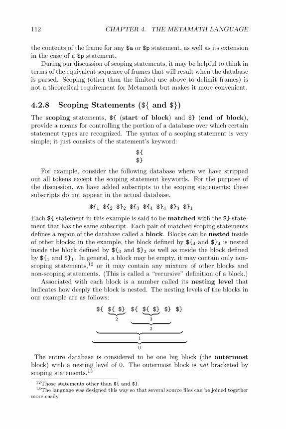
112 CHAPTER 4. THE METAMATH LANGUAGE
the contents of the frame for any $a or $p statement, as well as its extensionin the case of a $p statement.
During our discussion of scoping statements, it may be helpful to think interms of the equivalent sequence of frames that will result when the databaseis parsed. Scoping (other than the limited use above to delimit frames) isnot a theoretical requirement for Metamath but makes it more convenient.
4.2.8 Scoping Statements (${ and $})The scoping statements, ${ (start of block) and $} (end of block),provide a means for controlling the portion of a database over which certainstatement types are recognized. The syntax of a scoping statement is verysimple; it just consists of the statement’s keyword:
${
$}
For example, consider the following database where we have strippedout all tokens except the scoping statement keywords. For the purpose ofthe discussion, we have added subscripts to the scoping statements; thesesubscripts do not appear in the actual database.
${1 ${2 $}2 ${3 ${4 $}4 $}3 $}1
Each ${ statement in this example is said to be matched with the $} state-ment that has the same subscript. Each pair of matched scoping statementsdefines a region of the database called a block. Blocks can be nested insideof other blocks; in the example, the block defined by ${4 and $}4 is nestedinside the block defined by ${3 and $}3 as well as inside the block definedby ${1 and $}1. In general, a block may be empty, it may contain only non-scoping statements,12 or it may contain any mixture of other blocks andnon-scoping statements. (This is called a “recursive” definition of a block.)
Associated with each block is a number called its nesting level thatindicates how deeply the block is nested. The nesting levels of the blocks inour example are as follows:
${ ${ $}︸ ︷︷ ︸2
${ ${ $}︸ ︷︷ ︸3
$}
︸ ︷︷ ︸2
$}
︸ ︷︷ ︸1︸ ︷︷ ︸0
The entire database is considered to be one big block (the outermostblock) with a nesting level of 0. The outermost block is not bracketed byscoping statements.13
12Those statements other than ${ and $}.13The language was designed this way so that several source files can be joined together
more easily.

4.2. THE BASIC KEYWORDS 113
All non-scoping Metamath statements become recognized or active atthe place where they appear.14 Certain of these statement types becomeinactive at the end of the block in which they appear; these statement typesare:
$c, $v, $d, $e, and $f.
The other statement types remain active forever (i.e. through the end of thedatabase); they are:
$a and $p.
Any statement (of these 7 types) located in the outermost block will remainactive through the end of the database and thus are effectively “global”statements.
All $c statements must be placed in the outermost block. Since they aretherefore always global, they could be considered as belonging to both ofthe above categories.
The scope of a statement is the set of statements that recognize it asactive.
The concept of “active” is also defined for math symbols. Math symbols(constants and variables) become active in the $c and $v statements thatdeclare them. A variable becomes inactive when its declaration statementbecomes inactive. Because all $c statements must be in the outermost block,a constant will never become inactive after it is declared.
Redeclaration of Math Symbols
A variable may not be declared a second time while it is active, but it maybe declared again after it becomes inactive. This provides a convenientway to introduce “local” variables, i.e. temporary variables for use in theframe of an assertion or in a proof without keeping them around forever. Apreviously declared variable may not be redeclared as a constant.
A constant may not be redeclared. And, as mentioned above, constantsmust be declared in the outermost block.
The reason variables may have limited scope but not constants is that anassertion ($a or $p statement) remains available for use in proofs through theend of the database. Variables in an assertion’s frame may be substitutedwith whatever is needed in a proof step that references the assertion, whereasconstants remain fixed and may not be substituted with anything. Theparticular token used for a variable in an assertion’s frame is irrelevantwhen the assertion is referenced in a proof, and it doesn’t matter if thattoken is not available outside of the referenced assertion’s frame. Constants,however, must be globally fixed.
14To keep things slightly simpler, we do not bother to define the concept of “active”for the scoping statements.

114 CHAPTER 4. THE METAMATH LANGUAGE
In the present version of the Metamath language, there is no theoreticalbenefit for the feature allowing variables to be active for limited scopesrather than global. It is just a convenience that allows them, for example,to be locally grouped together with their corresponding $f variable-typedeclarations.15
Frames Revisited
Now that we have covered scoping, we will look at how an arbitrary Meta-math database can be converted to the simple sequence of extended framesdescribed on p. 111. This is also how Metamath stores the database in-ternally when it reads in the database source. The method is simple.First, we collect all constant and variable ($c and $v) declarations in thedatabase, ignoring duplicate declarations of the same variable in differentscopes. We then put our collected $c and $v declarations at the beginningof the database, so that their scope is the entire database. Next, for eachassertion in the database, we determine its frame and extended frame. Theextended frame is simply the $f, $e, and $d statements that are active. Theframe is the extended frame with all optional hypotheses removed.
An equivalent way of saying this is that the extended frame of an asser-tion is the collection of all $f, $e, and $d statements whose scope includesthe assertion, in the order they appear.
4.3 The Anatomy of a Proof
Each provable assertion ($p statement) in a database must include a proof.The proof is located between the $= and $. keywords in the $p statement.
In the basic Metamath language, a proof is a sequence of statement la-bels. This label sequence serves as a set of instructions that the Metamathprogram uses to construct a series of math symbol sequences. The construc-tion must ultimately result in the math symbol sequence contained betweenthe $p and $= keywords of the $p statement. Otherwise, the Metamathprogram will consider the proof incorrect, and it will notify you with anappropriate error message when you ask it to verify the proof.16 Each labelin a proof is said to reference its corresponding statement.
Associated with any assertion ($p or $a statement) is a set of hypotheses($f or $e statements) that are active with respect to that assertion. Some are
15A future version of the Metamath language may extend the language to include truelocal variables as well as local constants. I have not decided upon the best way to do thisor even if it should be done at all; the main issue is whether the benefits offset greaterconfusion in learning the language. In any case, the rules for the present language werechosen to let existing databases be compatible with any future language extensions.
16To make the loading faster, the Metamath program does not automatically verifyproofs when you read in a database unless you use the /verify qualifier. After a databasehas been read in, you may use the verify proof * command to verify proofs.
4.3. THE ANATOMY OF A PROOF 115
mandatory and the others are optional. You should review these conceptsif necessary.
Each label in a proof must be either the label of a previous assertion ($aor $p statement) or the label of an active hypothesis ($e or $f statement)of the $p statement containing the proof. Hypothesis labels may referenceboth the mandatory and the optional hypotheses of the $p statement.
The label sequence in a proof specifies a construction in reverse Pol-ish notation (RPN). You may be familiar with RPN if you have usedHewlett-Packard or similar hand-held calculators. In the calculator analogy,a hypothesis label is like a number and an assertion label is like an operation.On an RPN calculator, an operation takes one or more previous numbersin an input sequence, performs a calculation on them, and replaces thosenumbers and itself with the result of the calculation. For example, the inputsequence 2, 2,+ on an RPN calculator results in 4, and the input sequence1, 2, 2,+,+ results in 1, 4,+ which results in 5.
Understanding how RPN is processed involves the concept of a stack,which can be thought of as a set of temporary memory locations that hold in-termediate results. When Metamath encounters a hypothesis label it placesor pushes the math symbol sequence of the hypothesis onto the stack. WhenMetamath encounters an assertion label, it associates the most recent stackentries with the mandatory hypotheses of the assertion, in the order wherethe most recent stack entry is associated with the last mandatory hypothesisof the assertion. It then determines what substitutions have to be made intothe variables of the assertion’s mandatory hypotheses to make them identi-cal to the associated stack entries. It then makes those same substitutionsinto the assertion itself. Finally, Metamath removes or pops the matchedhypotheses from the stack and pushes the substituted assertion onto thestack.
For the purpose of matching the mandatory hypothesis to the most recentstack entries, whether a hypothesis is a $e or $f statement is irrelevant.The only important thing is that a set of substitutions17 exist that allow amatch (and if they don’t, the proof verifier will let you know with an errormessage). The Metamath language is specified in such a way that if a setof substitutions exists, it will be unique. Specifically, the requirement thateach variable have a type specified for it with a $f statement ensures theuniqueness.
We will illustrate this with an example. Consider the following Metamathsource file:
$c ( ) -> wff $.
$v p q r s $.
wp $f wff p $.
wq $f wff q $.
17In the Metamath spec (Section 4.1), we use the singular term “substitution” to referto the set of substitutions we talk about here.

116 CHAPTER 4. THE METAMATH LANGUAGE
wr $f wff r $.
ws $f wff s $.
w2 $a wff ( p -> q ) $.
wnew $p wff ( s -> ( r -> p ) ) $= ws wr wp w2 w2 $.
This Metamath source example shows the definition and “proof” (i.e., con-struction) of a well-formed formula (wff) in propositional calculus. (Youmay wish to type this example into a file to experiment with the Metamathprogram.) The first two statements declare (introduce the names of) fourconstants and four variables. The next four statements specify the variabletypes, namely that each variable is assumed to be a wff. Statement w2 de-fines (postulates) a way to produce a new wff, ( p -> q ), from two givenwffs p and q. The mandatory hypotheses of w2 are wp and wq. Statementwnew claims that ( s -> ( r -> p ) ) is a wff given three wffs s, r, andp. More precisely, wnew claims that the sequence of ten symbols wff ( s
-> ( r -> p ) ) is provable from previous assertions and the hypothesesof wnew. Metamath does not know or care what a wff is, and as far asit is concerned wff is just an arbitrary constant symbol in a math symbolsequence. The mandatory hypotheses of wnew are wp, wr, and ws; wq isan optional hypothesis. In our particular proof, the optional hypothesis isnot referenced, but in general, any combination of active (i.e. optional andmandatory) hypotheses could be referenced. The proof of statement wnew
is the sequence of five labels starting with ws (step 1) and ending with w2
(step 5).When Metamath verifies the proof, it scans the proof from left to right.
We will examine what happens at each step of the proof. The stack startsoff empty. At step 1, Metamath looks up label ws and determines that itis a hypothesis, so it pushes the symbol sequence of statement ws onto thestack:
Stack location Contents
1 wff s
Metamath sees that the labels wr and wp in steps 2 and 3 are also hy-potheses, so it pushes them onto the stack. After step 3, the stack looks likethis:
Stack location Contents
3 wff p
2 wff r
1 wff s
At step 4, Metamath sees that label w2 is an assertion, so it must do someprocessing. First, it associates the mandatory hypotheses of w2, which arewp and wq, with stack locations 2 and 3, in that order. Metamath determinesthat the only possible way to make hypothesis wp match (become identical
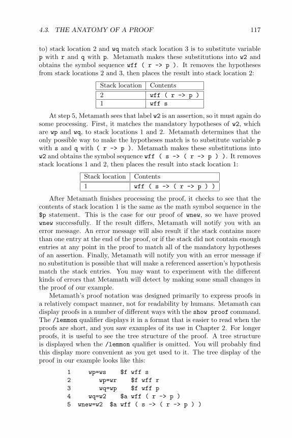
4.3. THE ANATOMY OF A PROOF 117
to) stack location 2 and wq match stack location 3 is to substitute variablep with r and q with p. Metamath makes these substitutions into w2 andobtains the symbol sequence wff ( r -> p ). It removes the hypothesesfrom stack locations 2 and 3, then places the result into stack location 2:
Stack location Contents
2 wff ( r -> p )
1 wff s
At step 5, Metamath sees that label w2 is an assertion, so it must again dosome processing. First, it matches the mandatory hypotheses of w2, whichare wp and wq, to stack locations 1 and 2. Metamath determines that theonly possible way to make the hypotheses match is to substitute variable p
with s and q with ( r -> p ). Metamath makes these substitutions intow2 and obtains the symbol sequence wff ( s -> ( r -> p ) ). It removesstack locations 1 and 2, then places the result into stack location 1:
Stack location Contents
1 wff ( s -> ( r -> p ) )
After Metamath finishes processing the proof, it checks to see that thecontents of stack location 1 is the same as the math symbol sequence in the$p statement. This is the case for our proof of wnew, so we have provedwnew successfully. If the result differs, Metamath will notify you with anerror message. An error message will also result if the stack contains morethan one entry at the end of the proof, or if the stack did not contain enoughentries at any point in the proof to match all of the mandatory hypothesesof an assertion. Finally, Metamath will notify you with an error message ifno substitution is possible that will make a referenced assertion’s hypothesismatch the stack entries. You may want to experiment with the differentkinds of errors that Metamath will detect by making some small changes inthe proof of our example.
Metamath’s proof notation was designed primarily to express proofs ina relatively compact manner, not for readability by humans. Metamath candisplay proofs in a number of different ways with the show proof command.The /lemmon qualifier displays it in a format that is easier to read when theproofs are short, and you saw examples of its use in Chapter 2. For longerproofs, it is useful to see the tree structure of the proof. A tree structureis displayed when the /lemmon qualifier is omitted. You will probably findthis display more convenient as you get used to it. The tree display of theproof in our example looks like this:
1 wp=ws $f wff s
2 wp=wr $f wff r
3 wq=wp $f wff p
4 wq=w2 $a wff ( r -> p )
5 wnew=w2 $a wff ( s -> ( r -> p ) )

118 CHAPTER 4. THE METAMATH LANGUAGE
The number to the left of each line is the step number. Following it isa hypothesis association, consisting of two labels separated by =. Tothe left of the = (except in the last step) is the label of a hypothesis of anassertion referenced later in the proof; here, steps 1 and 4 are the hypothesisassociations for the assertion w2 that is referenced in step 5. A hypothesisassociation is indented one level more than the assertion that uses it, so it iseasy to find the corresponding assertion by moving directly down until theindentation level decreases to one less than where you started from. To theright of each = is the proof step label for that proof step. The statementkeyword of the proof step label is listed next, followed by the content of thetop of the stack (the most recent stack entry) as it exists after that proofstep is processed. With a little practice, you should have no trouble readingproofs displayed in this format.
Our simple example shows the syntax construction of a formula thatmight be used as part of the construction of a “real” proof step that de-duces theorems from other theorems. In standard mathematics, this kindof construction is not considered a proper part of the proof at all, and itcertainly becomes rather boring after a while. To filter out syntax con-structions in the proof display, the show proof command has the qualifier/essential which you will probably use quite often in order to see just the“real” steps of the proof.
When verifying a proof, Metamath will check that no mandatory $d
statement of an assertion referenced in a proof is violated when substitutionsare made to the variables in the assertion. For details see Section 4.1.4 or4.2.4.
4.3.1 The Concept of Unification
During the course of verifying a proof, when Metamath encounters an asser-tion label, it associates the mandatory hypotheses of the assertion with thetop entries of the RPN stack. Metamath then determines what substitu-tions it must make to the variables in the assertion’s mandatory hypothesesin order for these hypotheses to become identical to their correspondingstack entries. This process is called unification. (We also informally usethe term “unification” to refer to a set of substitutions that results from theprocess, as in “two unifications are possible.”) After the substitutions aremade, the hypotheses are said the be unified.
If no such substitutions are possible, Metamath will consider the proofincorrect and notify you with an error message.
The general algorithm for unification described in the literature is some-what complex. However, in the case of Metamath it is trivial because ofthe requirement that each variable have its type specified with a $f hypoth-esis and that each $f hypothesis have the restricted syntax of a constantfollowed by a variable. The constant in the $f hypothesis must match thefirst symbol of the corresponding RPN stack entry (which will be also be a

4.4. EXTENSIONS TO THE METAMATH LANGUAGE 119
constant), so only possible match for the variable in the $f hypothesis is thesequence of symbols in the stack entry after the initial constant.
In the Proof Assistant, a more general unification algorithm is used.While a proof is being developed, sometimes not enough information is avail-able to determine a unique unification. In this case Metamath will ask youto pick the correct one.
4.4 Extensions to the Metamath Language
4.4.1 Comments in the Metamath Language
The commenting feature allows you to annotate the contents of a database.Just as with most computer languages, comments are ignored for the purposeof interpreting the contents of the database. Comments effectively act asadditional white space between tokens when a database is parsed.
A comment may be placed between any two tokens in a source file.Comments have the following syntax:
$( text $)
Here, text is a string, possibly empty, of any characters in Metamath’s char-acter set (p. 92), except that the character strings $( and $) may not appearin text. Thus nested comments are not permitted:18 Metamath will com-plain if you give it
$( This is a $( nested $) comment. $)
(To compensate for this behavior, I often change all $’s to @’s in sections ofMetamath code I wish to comment out.)
Math Symbols and Labels Inside Comments
Inside of comments, a string of tokens enclosed in grave accents (‘) will beconverted to standard mathematical symbols during LATEX output typeset-ting, according to the information in the special $t comment in the database,as described in Appendix A. The first ‘ causes the output processor to entermath mode and the second one exits it. Two consecutive grave accents ‘‘are treated as a single actual grave accent (both inside and outside of mathmode) and will not cause the output processor to enter or exit math mode.
Outside of math mode, any token preceded by a tilde (~) will be format-ted in typewriter font, and the tilde removed, to make them stand it fromthe rest of the text. This formatting will be applied from all characters afterthe tilde up to the first white space. This formatting mode is called label
18Computer languages have differing standards for nested comments, and rather thanpicking one it was felt simplest not to allow them at all, at least in the current version ofMetamath (0.07.30).

120 CHAPTER 4. THE METAMATH LANGUAGE
mode. If a literal tilde is desired (outside of math mode), use two tildes ina row to represent it.
These markup features have to do only with how the comments are type-set, and have no effect on how Metamath verifies the database. The improperuse of them may result in incorrectly typeset output, but no Metamath errormessages will result during the read and verify proof commands. (How-ever, the new write theorem_list command, added in version 0.07.30 ofthe Metamath program, will check for markup errors as a side-effect of itshtml generation.)
Section 5.7 has instructions for creating LATEX output.
Math Symbols In Comments
The grave accent ‘ tells Metamath to switch a comment to math mode.In this mode, the characters following the ‘ are interpreted as a sequenceof math symbol tokens separated by white space. The tokens are lookedup in the $t comment and if found, they will be replaced by the standardmathematical symbols that they correspond to before being placed in thetypeset output file. If not found, the symbol will be output as is and awarning will be issued. The tokens do not have to be active in the database,although a warning will be issued if they are not declared with $c or $v
statements.The comment will stay in math mode until a second ‘ is found or the
end of the comment is reached. Here is an example of its use:
$( Pierce’s axiom, ‘ ( ( ph -> ps ) -> ph ) -> ph ‘ ,
is not very intuitive. $)
becomes
$( Pierce’s axiom, ((ϕ→ ψ)→ ϕ)→ ϕ, is not very intuitive. $)
Note that the math symbol tokens must be surrounded by white space.White space should also surround the ‘ delimiters.
The math mode feature also gives you a quick and easy way to generatetext containing mathematical symbols, independently of the intended pur-pose of Metamath. To do this, simply create your text with grave accentssurrounding your formulas, after making sure that your math symbols aremapped to LATEX symbols as described in Appendix A. It is easier if youstart with a database with predefined symbols such as set.mm. Use yourgrave-quoted math string to replace an existing comment, then typeset thestatement corresponding to that comment following the instructions fromthe help tex command in the Metamath program. You will then probablywant to edit the resulting file with a text editor to fine tune it to your exactneeds.

4.4. EXTENSIONS TO THE METAMATH LANGUAGE 121
Label References in Comments
Outside of math mode, a tilde ~ indicates to Metamath’s output processorthat the token that follows (i.e. the characters up to the next white space)represents a statement label. Whether or not the token is an actual state-ment label is not checked, and the token does not have to have the correctsyntax for a label; no error messages will be produced. The only effect ofthe label mode on the output is that typewriter font will be used for thetokens that are placed in the LATEX output file.
(On the other hand, the tokens after the tilde must be actual labels forcorrect output of html, described in the next section, and error messageswill be issued during that output if they aren’t.)
4.4.2 Comment Markup Notation for HTML
The automated generation of html web pages (Section 5.8) is new in version0.07.30 of the Metamath program. The comment markup notation for LATEXalso applies to html, and some additional features specifically for html wereadded. These markup features (including those reused from LATEX) are thefollowing.
‘ math-symbol math-symbol ... ‘ (math symbols enclosed in grave ac-cents i.e. backticks) - Use graphical math-symbols in the html output.Inside of a math-symbol, ‘‘ means literal ‘.
~ label (tilde followed by a label) - Use a hyperlink in the html outputthat links to the web page for statement label. Exception: if labelbegins with http://, it is assumed to be a url (which is used as-is,except that a ~ in the url should be specified with ~~). Only $a
and $p statement labels may be used, since web pages for $e and $f
statements are not generated.
[author] - Link to a bibliographical reference. See help html andhelp write bibliography in the Metamath program for more infor-mation. See also Sections 5.8.1 and 5.8.3.
$t - Flag the comment as the special one containing LATEX and/orhtml typesetting definitions. See Section 5.8.1 and Appendix A.
_ (underscore) - Italicize text starting from space_non-space (i.e. _
with a space before it and a non-space character after it) until thenext non-space_space. Normal punctuation (e.g. a trailing comma orperiod) is ignored when determining space.
_ (underscore) - non-space_non-space-string, where non-space-stringis a string of non-space characters, will make non-space-string becomea subscript.

122 CHAPTER 4. THE METAMATH LANGUAGE
It is recommended that spaces surround any ~ and ‘ tokens in the com-ment and that a space follow the label after a ~ token. This will makeglobal substitutions to change labels and symbol names much easier andalso eliminate any future chance of ambiguity. Spaces around these tokensare automatically removed in the final output to conform with normal rulesof punctuation; for example, a space between a trailing ‘ and a left paren-thesis will be removed.
The [author] notation will also create an entry in the bibliography cross-reference file generated by write bibliography (Section 5.8.3). For this towork properly, the surrounding comment must be formatted as follows:
keyword label noise-word [author] p. number
for example
Theorem 5.2 of [Monk] p. 223
The keyword is not case sensitive and must be one of the following:
theorem lemma definition compare proposition corollary
axiom rule remark exercise problem notation example
property figure postulate equation scheme chapter
The optional label may consist of more than one (non-keyword and non-noise-word) word. The optional noise-word is one of:
of in from on
and is ignored when the cross-reference file is created. The write biblio-
graphy command will perform error checking to verify the above format.A good way to become familiar with the markup notation is to look at
the extensive examples in the set.mm database.
4.4.3 Including Other Files in a Metamath Source File
The keywords $[ and $] specify a file to be included at that point in aMetamath source file. The syntax for including a file is as follows:
$[ file-name $]
The file-name should be a single token with the same syntax as a mathsymbol (i.e., all 93 printable characters other than $ are allowed, subjectto the file-naming limitations of your operating system). Comments mayappear between the $[ and $] keywords. Included files may include otherfiles, which may in turn include other files, and so on.
For example, suppose you want to use the set theory database as thestarting point for your own theory. The first line in your file could be
$[ set.mm $]

4.4. EXTENSIONS TO THE METAMATH LANGUAGE 123
All of the information (axioms, theorems, etc.) in set.mm and any files thatit includes will become available for you to reference in your file. This canhelp make your work more modular. A drawback to including files is that ifyou change the name of a symbol or the label of a statement, you must alsoremember to update any references in any file that includes it.
The naming conventions for included files are the same as those of youroperating system.19 For compatibility among operating systems, you shouldkeep the file names as simple as possible. A good convention to use is file.mmwhere file is eight characters or less, in lower case.
There is no limit to the nesting depth of included files. One thing thatyou should be aware of is that if two included files themselves include acommon third file, only the first reference to this common file will be readin. This allows you to include two or more files that build on a commonstarting file without having to worry about label and symbol conflicts thatwould occur if the common file were read in more than once. (In fact, if afile includes itself, the self reference will be ignored, although of course itwould not make any sense to do that.) This feature also means, however,that if you try to include a common file in several inner blocks, the resultmight not be what you expect, since only the first reference will be replacedwith the included file (unlike the include statement in most other computerlanguages). Thus you would normally include common files only in theoutermost block.
4.4.4 Compressed Proof Format
The proof notation presented in Section 4.3 is called a normal proof andin principle is sufficient to express any proof. However, proofs often con-tain steps and subproofs that are identical. This is particularly true intypical Metamath applications, because Metamath requires that the mathsymbol sequence (usually containing a formula) at each step be separatelyconstructed, that is, built up piece by piece. As a result, a lot of repetitionoften results. The compressed proof format allows Metamath to takeadvantage of this redundancy to shorten proofs.
The specification for the compressed proof format is given in Appendix B.Normally you need not concern yourself with the details of the com-
pressed proof format, since the Metamath program will allow you to convertfrom the normal format to the compressed format with ease, and will also au-tomatically convert from the compressed format when proofs are displayed.The overall structure of the compressed format is as follows:
19On the Macintosh, prior to Mac OS X, a colon is used to separate disk and foldernames from your file name. For example, volume:file-name refers to the root di-rectory, volume:folder-name:file-name refers to a folder in root, and volume:folder-name:. . . :file-name refers to a deeper folder. A simple file-name refers to a file in thefolder from which you launch the Metamath application. Under Mac OS X and later,the Metamath program is run under the Terminal application, which conforms to Unixnaming conventions.
124 CHAPTER 4. THE METAMATH LANGUAGE
$= ( label-list ) compressed-proof $.
The first ( serves as a flag to Metamath that a compressed proof follows.The label-list includes all statements referred to by the proof except themandatory hypotheses. The compressed-proof is a compact encoding of theproof, using upper case letters, and can be thought of as a large integer inbase 26. White space inside of compressed-proof is optional and is ignored.
It is important to note that the order of the mandatory hypotheses ofthe statement being proved must not be changed if the compressed proofformat is used, otherwise the proof will become incorrect. The reason forthis is that the mandatory hypotheses are not mentioned explicitly in thecompressed proof in order to make the compression more efficient. If youwish to change the order of mandatory hypotheses, you must first convertthe proof back to normal format using the save proof statement /normal
command. Later, you can go back to compressed format with save proof
statement /compressed.During error checking with the verify proof command, an error found
in the a compressed proof may point to a character in compressed-proof,which may not be very meaningful to you. In this case, try to save proof
/normal first, then do the verify proof again. In general, it is best tomake sure a proof is correct before saving it in compressed format, becausesevere errors are less likely to be recoverable than in normal format.
4.4.5 Specifying Unknown Proofs or Subproofs
In a proof under development, any step or subproof that is not yet knownmay be represented with a single ?. For the purposes of parsing the proof, the? will push a single entry onto the RPN stack just as if it were a hypothesis.While developing a proof with the Proof Assistant, a partially developedproof may be saved with the save new_proof command, and ?’s will beplaced at the appropriate places.
All $p statements must have proofs, even if they are entirely unknown.Before creating a proof with the Proof Assistant, you should specify a com-pletely unknown proof as follows:
label $p statement $= ? $.
The verify proof command will check the known portions of a partialproof for errors, but will warn you that the statement has not been proved.
Note that partially developed proofs may be saved in compressed formatif desired. In this case, you will see one or more ?’s in the compressed-proofpart.
4.5. APPENDIX: AXIOMS VS. DEFINITIONS 125
4.5 Appendix: Axioms vs. Definitions
Metamath makes no distinction between axioms and definitions. The $a
statement is used for both. At first, this may seem puzzling. In the mindsof many mathematicians, the distinction is clear, even obvious, and hardlyworth discussing. A definition is considered to be merely an abbreviationthat can be replaced by the expression for which it stands; although unlessone actually does this, to be precise that one should say that a theoremis a consequence of the axioms and the definitions that are used in theformulation of the theorem [4, p. 20].
What is a definition? In its simplest form, a definition introduces anew symbol and provides an unambiguous rule to transform an expressioncontaining the new symbol to one without it. The concept of a “properdefinition” (as opposed to a creative definition) that is usually agreed uponis (1) the definition should not strengthen the language and (2) any symbolsintroduced by the definition should be eliminable from the language [42]. Inother words, they are mere typographical conveniences that do not belongto the system and are theoretically superfluous. This may seem obvious, butin fact the nature of definitions can be subtle, sometimes requiring difficultmetatheorems to establish that they are not creative.
A more conservative stance was taken by logician S. Lesniewski.
Lesniewski regards definitions as theses of the system. In thisrespect they do not differ either from the axioms or from theo-rems, i.e. from the theses added to the system on the basis of therule of substitution or the rule of detachment [modus ponens].Once definitions have been accepted as theses of the system, itbecomes necessary to consider them as true propositions in thesame sense in which axioms are true [32].
Let us look at some simple examples of definitions in propositional cal-culus. Consider the definition of logical or (disjunction): “P ∨ Q denotes¬P → Q (not P implies Q).” It is very easy to recognize a statement mak-ing use of this definition, because it introduces the new symbol ∨ that didnot previously exist in the language. It is easy to see that no new theoremsof the original language will result from this definition.
Next, consider a definition that eliminates parentheses: “P → Q → Rdenotes P → (Q → R).” This is more subtle, because no new symbols areintroduced. The reason this definition is considered proper is that no newsymbol sequences that are valid wffs (well-formed formulas) in the originallanguage will result from the definition, since “P → Q→ R” is not a wff inthe original language. Here, we implicitly make use of the fact that there isa decision procedure that allows us to determine whether or not a symbolsequence is a wff, and this fact allows us to use symbol sequences that arenot wffs to represent other things (such as wffs) by means of the definition.However, to justify the definition as not being creative we need to prove that

126 CHAPTER 4. THE METAMATH LANGUAGE
“P → Q→ R” is in fact not a wff in the original language, and this is moredifficult than in the case where we simply introduce a new symbol.
What constitutes a definition versus an axiom is sometimes arbitrary inmathematical literature. For example, the connectives ∨ (or), ∧ (and),and ↔ (equivalent to) in propositional calculus are usually considered de-fined symbols that can be used as abbreviations for expressions containingthe “primitive” connectives → and ¬. This is the way we treat them in thestandard logic and set theory database set.mm. However, the first three con-nectives can also be considered “primitive,” and axiom systems have beendevised that treat all of them as such. For example, [17, p. 35] presents onewith 15 axioms, some of which in fact coincide with what we have chosen tocall definitions in set.mm. In certain subsets of classical propositional calcu-lus, such as the intuitionist fragment, it can be shown that one cannot makedo with just → and ¬ but must treat additional connectives as primitive inorder for the system to make sense.20
In set theory, recursive definitions define a newly introduced symbol interms of itself. The justification of recursive definitions, using several “recur-sion theorems,” is the usually one of the first sophisticated proofs a studentencounters when learning set theory, and there is a significant amount ofimplicit metalogic behind a recursive definition even though the definitionitself is typically simple to state. It is, however, possible to substitute onekind of complexity for another. We can eliminate the need for metalog-ical justification by defining the operation directly with an explicit (butcomplicated) expression, then deriving the recursive definition directly as atheorem, using a recursion theorem “in reverse.” We do this in set.mm, asfollows.
In set.mm our goal was to introduce almost all definitions in the form oftwo expressions connected by either ↔ or =, where the thing being defineddoes not appear on the right hand side. Quine calls this form “a genuineor direct definition” [48, p. 174], which makes the definitions very easy toeliminate and the metalogic needed to justify them as simple as possible.We achieved this goal in almost all cases. Sometimes this makes the defini-tions more complex and less intuitive. For example, the traditional way todefine addition of natural numbers is to define an operation called successor(which means “plus one” and is denoted by “suc”), then define additionrecursively with the two definitions n+ 0 = n and m+ sucn = suc(m+ n).Although this definition seems simple and obvious, the method to eliminatethe definition is not obvious: in the second part of the definition, additionis defined in terms of itself. By eliminating the definition, we don’t meanrepeatedly applying it to specific m and n but rather showing the explicit,closed-form set-theoretical expression that m+ n represents, that will workfor any m and n and that does not have a + sign on its right-hand side. For
20Two nice systems that make the transition from intuitionistic and other weak frag-ments to classical logic just by adding axioms are given in [50].

4.5. APPENDIX: AXIOMS VS. DEFINITIONS 127
a recursive definition like this not to be circular (creative), there are somehidden, underlying assumptions we must make, for example that the natu-ral numbers have a certain kind of order. In set.mm we chose to start withthe direct (though complex and nonintuitive) definition then derive fromit the standard recursive definition.21 The end result is the same, but wecompletely eliminate the rather complex metalogic that justifies the recur-sive definition. (For a mathematician, recursive definitions are more efficientand intuitive than direct ones once the metalogic has been learned or pos-sibly just accepted as correct. However, it was felt that direct definitionin set.mm maximizes rigor by minimizing metalogic. It can be eliminatedeffortlessly, something difficult to do with a recursive definition.)
21The closed-form definition used in set.mm for the addition operation on ordinals (ofwhich natural numbers are a subset) is
df-oadd $a `+o = { 〈 〈x , y 〉 , z 〉 | ( (x∈On∧ y ∈On )∧ z= ( rec ( { 〈w , v 〉 | v= sucw }, x ) ‘ y ) ) }
Here, the abstraction class of nested ordered pairs is defined by df-oprab in set.mm, andrec is a “recursion operator” with the definition
df-rfg $a ` rec (F ,A ) =⋃{ f | ∃x (x∈On∧ ( f Fnx∧∀ y ( y ∈x→ ( f ‘ y ) = ( { 〈 g , z
〉 | ( ( g=∅∧ z=A )∨ (¬ ( g=∅∨Lim dom g )∧ z= (F ‘ ( g ‘⋃
dom g ) ) )∨( Lim dom g ∧ z=
⋃ran g ) ) } ‘ ( f � y ) ) ) ) ) }
which can be further broken down with definitions shown in Section 3.4.3. You maybe surprised at the complexity of what seems like such a simple notion. From thesedefinitions the simpler, more intuitive recursive definition is derived as a set of theorems.
128 CHAPTER 4. THE METAMATH LANGUAGE

Chapter 5
The Metamath Program
This chapter provides a reference manual for the Metamath program.Current instructions for obtaining and installing the Metamath program
can be found at the http://metamath.org web site. For Windows, there isa pre-compiled version called metamath.exe. For Unix, Linux, and Mac OSX (which we will refer to collectively as “Unix”), the Metamath programcan be compiled from its source code with the command
gcc *.c -o metamath
using the gcc c compiler available on those systems.In the command syntax descriptions below, fields enclosed in square
brackets [ ] are optional. File names may be optionally enclosed in singleor double quotes. This is useful if the file name contains slashes (/), suchas in Unix path names, that might be confused with Metamath commandqualifiers.
5.1 Invoking Metamath
Unix, Linux, and Mac OS X have a command-line interface called thebash shell. (In Mac OS X, select the Terminal application from Applica-tions/Utilities.) To invoke Metamath from the bash shell prompt, assumingthat the Metamath program is in the current directory, type
bash$ ./metamath
To invoke Metamath from a Windows DOS or Command Prompt, as-suming that the Metamath program is in the current directory (or in adirectory included in the Path system environment variable), type
C:\metamath>metamath
129

130 CHAPTER 5. THE METAMATH PROGRAM
To use command-line arguments at invocation, the command-line argu-ments should be a list of Metamath commands, surrounded by quotes ifthey contain spaces. In Windows, the surrounding quotes must be double(not single) quotes. For example, to read the database file set.mm, verifyall proofs, and exit the program, type (under Unix)
bash$ ./metamath ’read set.mm’ ’verify proof *’ exit
Note that in Unix, any directory path with /’s must be surrounded by quotesso Metamath will not interpret the / as a command qualifier. So if set.mmis in the /tmp directory, use for the above example
bash$ ./metamath ’read "/tmp/set.mm"’ ’verify proof *’ exit
For convenience, if the command-line has one argument and no spacesin the argument, the command is implicitly assumed to be read. In thisone special case, /’s are not interpreted as command qualifiers, so you don’tneed quotes around a Unix file name. Thus
bash$ ./metamath /tmp/set.mm
and
bash$ ./metamath "read ’/tmp/set.mm’"
are equivalent.
5.2 Controlling Metamath
The Metamath program was first developed on a vax/vms system, andsome aspects of its command line behavior reflect this heritage. Hopefullyyou will find it reasonably user-friendly once you get used to it.
Each command line is a sequence of English-like words separated byspaces, as in show settings. Command words are not case sensitive, andonly as many letters are needed as are necessary to eliminate ambiguity;for example, sh se would work for the command show settings. In somecases arguments such as file names, statement labels, or symbol names arerequired; these are case-sensitive (although file names may not be on someoperating systems).
A command line is entered by typing it in then pressing the return (enter)key. To find out what commands are available, type ? at the MM> prompt.To find out the choices at any point in a command, press return and youwill be prompted for them. The default choice (the one selected if you justpress return) is shown in brackets (<>).
You may also type ? in place of a command word to force Metamathto tell you what the choices are. The ? method won’t work, though, if a
5.2. CONTROLLING METAMATH 131
non-keyword argument such as a file name is expected at that point, becausethe program will think that ? is the value of the argument.
Some commands have one or more optional qualifiers which modify thebehavior of the command. Qualifiers are preceded by a slash (/), such as inread set.mm / verify. Spaces are optional around the /. If you need touse a slash in a command argument, as in a Unix file name, put single ordouble quotes around the command argument.
The open log command will save everything you see on the screen andis useful to help you recover should something go wrong in a proof, or if youwant to document a bug.
If a command responds with more than a screenful, you will be promptedto <return> to continue, Q to quit, or S to scroll to end. Q or q(not case-sensitive) will complete the command internally but will suppressfurther output until the next MM> prompt. s will suppress further pausinguntil the next MM> prompt. After the first screen, you are also presentedwith the choice of b to go back a screenful. Note that b may also be enteredat the MM> prompt immediately after a command to scroll back through theoutput of that command.
A command line enclosed in quotes is executed by your operating system.See Section 5.2.12.
Warning: Pressing ctrl-c will abort the Metamath program uncondi-tionally. This means any unsaved work will be lost.
5.2.1 exit Command
Syntax: exit [/force]This command exits from Metamath. If there have been changes to the
source with the save proof or save new_proof commands, you will begiven an opportunity to write source to permanently save the changes.
In Proof Assistant mode, the exit command will return to the MM>
prompt. If there were changes to the proof, you will be given an oppor-tunity to save new_proof.
The quit command is a synonym for exit.Optional qualifier: /force - Do not prompt if changes were not saved.
This qualifier is useful in submit command files (Section 5.2.4) to ensurepredictable behavior.
5.2.2 open log Command
Syntax: open log file-nameThis command will open a log file that will store everything you see on
the screen. It is useful to help recovery from a mistake in a long ProofAssistant session, or to document bugs.
The log file can be closed with close log. It will automatically be closedupon exiting Metamath.

132 CHAPTER 5. THE METAMATH PROGRAM
5.2.3 close log Command
Syntax: close log
The close log command closes a log file if one is open. See also open
log.
5.2.4 submit Command
Syntax: submit filenameThis command causes further command lines to be taken from the spec-
ified file. Note that any line beginning with an exclamation point (!) istreated as a comment (i.e. ignored). Also note that the scrolling of thescreen output is continuous, so you may want to open a log file (see open
log) to record the results that fly by on the screen. After the lines in thefile are exhausted, Metamath returns to its normal user interface mode.
Currently, the submit command is not recursive. In other words, submitcommands are not allowed inside of a command file.
5.2.5 erase Command
Syntax: eraseThis command will reset Metamath to its starting state, deleting any
database that was read in. If there have been changes to the source withthe save proof or save new_proof commands, you will be given an oppor-tunity to write source to permanently save the changes.
5.2.6 set echo Command
Syntax: set echo on or set echo off
The set echo on command will cause command lines to be echoed withany abbreviations expanded. While learning the Metamath commands, thisfeature will show you the exact command that your abbreviated input cor-responds to.
5.2.7 set scroll Command
Syntax: set scroll prompted or set scroll continuous
The Metamath command line interface starts off in the prompted mode,which means that you will prompted to continue or quit after each full screenin a long listing. In continuous mode, long listings will be scrolled withoutpausing.
5.2.8 set width Command
Syntax: set width number

5.2. CONTROLLING METAMATH 133
Metamath assumes the width of your screen is 79 characters (chosenbecause the Command Prompt in Windows XP has a wrapping bug atcolumn 80). If your screen is wider or narrower, this command allows you tochange this default screen width. A larger width is advantageous for loggingproofs to an output file to be printed on a wide printer. A smaller width maybe necessary on some terminals; in this case, the wrapping of the informationmessages may sometimes seem somewhat unnatural, however. In LATEX,there is normally a maximum of 61 characters per line with typewriter font.(The examples in this book were produced with 61 characters per line.)
5.2.9 set height Command
Syntax: set height numberMetamath assumes your screen height is 24 lines of characters. If your
screen is taller or shorter, this command lets you to change the number oflines at which the display pauses and prompts you to continue.
5.2.10 beep Command
Syntax: beepThis command will produce a beep. By typing it ahead after a long-
running command has started, it will alert you that the command is finished.For convenience, b is an abbreviation for beep.
Note: If b is typed at the MM> prompt immediately after the end of amultiple-page display paged with “Press <return> for more...” prompts,then the b will back up to the previous page rather than perform the beep
command. In that case you must type the unabbreviated beep form of thecommand.
5.2.11 more Command
Syntax: more filenameThis command will display the contents of an ascii file on your screen.
(This command is provided for convenience but is not very powerful. SeeSection 5.2.12 to invoke your operating system’s command to do this, suchas the more command in Unix.)
5.2.12 Operating System Commands
A line enclosed in single or double quotes will be executed by your computer’soperating system if it has a command line interface. For example, on avax/vms system, MM> ’dir’ will print disk directory contents. Note thatthis feature will not work on the Macintosh prior to Mac OS X, which doesnot have a command line interface.
For your convenience, the trailing quote is optional.

134 CHAPTER 5. THE METAMATH PROGRAM
5.2.13 Size Limitations in Metamath
In general, there are no fixed, predefined limits on how many labels, tokens,statements, etc. that you may have in a database file. The Metamath pro-gram uses 32-bit variables (64-bit on 64-bit CPUs) as indices for almost allinternal arrays, which are allocated dynamically as needed.
5.3 Reading and Writing Files
The following commands create new files: the open commands; the write
commands; the /html, /alt_html, /brief_html, /brief_alt_html quali-fiers of show statement, and midi. The following commands append to filespreviously opened: the /tex qualifier of show proof and show new_proof;the /tex and /simple_tex qualifiers of show statement; the close com-mands; and all screen dialog between open log and close log.
The commands that create new files will not overwrite an existing file-name but will rename the existing one to filename~1. An existing filename~1is renamed filename~2, etc. up to filename~9. An existing filename~9 isdeleted. This makes recovery from mistakes easier but also will clutter upyour directory, so occasionally you may want to clean up (delete) these ~nfiles.
5.3.1 read Command
Syntax: read file-name [/verify]This command will read in a Metamath language source file and any
included files. Normally it will be the first thing you do when enteringMetamath. Statement syntax is checked, but proof syntax is not checked.Note that the file name may be enclosed in single or double quotes; this isuseful if the file name contains slashes, as might be the case under Unix.
If you are getting an “?Expected VERIFY” error when trying to read aUnix file name with slashes, you probably haven’t quoted it.
If you are prompted for the file name (by pressing return after read) youshould not put quotes around it, even if it is a Unix file name with slashes.
Optional command qualifier:/verify - Verify all proofs as the database is read in. This qualifier will
slow down reading in the file. See verify proof for more information onfile error-checking.
See also erase.
5.3.2 write source Command
Syntax: write source filename [/clean]This command will write the contents of a Metamath database into a
file. Note: The present version of Metamath (0.07.30) will not split the
5.4. SHOWING STATUS AND STATEMENTS 135
database into its constituent source files included with $[ and $] keywords.A future version is planned to properly separate all constituent files.
Optional command qualifier (primarily intended to assist web site up-dates):
/clean - Suppresses (deletes) the output of any theorem that has beenflagged with a question mark (?) placed in or in place of the date commentfield at the end of its proof, for example “$( [?31-Oct-00] $).” This letsyou strip out proofs under development so that a “clean” version of thedatabase can be generated for official release. Note: Currently, hypothesesare not stripped, only $p statements. Spurious date comment fields of thesuppressed theorems may also remain. Be careful to use a different namefor the /clean version so that your work in progress won’t be destroyed.
5.4 Showing Status and Statements
5.4.1 show settings Command
Syntax: show settings
This command shows the state of various parameters.
5.4.2 show memory Command
Syntax: show memory
This command shows the available memory left. It is not be meaningfulon most modern operating systems, which have virtual memory.
5.4.3 show labels Command
Syntax: show labels label-match [/all] [/linear]This command shows the labels of $a and $p statements that match label-
match. A * in label-match matches zero or more characters. For example,*abc*def will match all labels containing abc and ending with def.
Optional command qualifier:/all - Include matches for $e and $f statement labels./linear - Display only one label per line. This can be useful for building
scripts in conjunction with the utilities under the tools command.
5.4.4 show statement Command
Syntax: show statement label [qualifiers (see below)]This command provides information about a statement. Only statements
that have labels ($f, $e, $a, and $p) may be specified. If label containswildcard (*) characters, all matching statements will be displayed in theorder they occur in the database.
Optional qualifiers (only one qualifier at a time is allowed):

136 CHAPTER 5. THE METAMATH PROGRAM
/comment - This qualifier includes the comment that immediately pre-cedes the statement.
/full - Show complete information about each statement, and show allstatements matching label (including $e and $f statements).
/tex - This qualifier will write the statement information to the LATEXfile previously opened with open tex. See Section 5.7.
/simple_tex - The same as /tex, except that LATEX macros are not usedfor formatting equations, allowing easier manual edits of the output for slidepresentations, etc.
/html, /alt_html, /brief_html, /brief_alt_html - These qualifiersinvoke a special mode of show statement that creates a web page for thestatement. They may not be used with any other qualifier. See Section 5.8or help html in the program.
5.4.5 search Command
Syntax: search label-match "symbol-match” [/ all] [/ comments]This command searches all $a and $p statements matching label-match
for occurrences of symbol-match. A * in label-match matches any label char-acter. A $* in symbol-match matches any sequence of symbols. The symbolsin symbol-match must be separated by white space. The quotes surround-ing symbol-match may be single or double quotes. For example, search
b* "-> $* ch" will list all statements whose labels begin with b and con-tain the symbols -> and ch surrounding any symbol sequence (including nosymbol sequence). The wildcards ? and $? are also available to matchindividual characters in labels and symbols respectively; see help search
in the Metamath program for details on their usage.Optional command qualifiers:/ all - Also search $e and $f statements./ comments - Search the comment that immediately precedes each label-
matched statement for symbol-match. In this case symbol-match is an arbi-trary, non-case-sensitive character string. Quotes around symbol-match areoptional if there is no ambiguity.
5.5 Displaying and Verifying Proofs
5.5.1 show proof Command
Syntax: show proof label [qualifiers (see below)]This command displays the proof of the specified $p statement in various
formats. The label may contain wildcard ($*) characters to match multiplestatements. Without any qualifiers, only the logical steps will be shown (i.e.syntax construction steps will be omitted), in an indented format.

5.5. DISPLAYING AND VERIFYING PROOFS 137
Most of the time, you will use show proof label to see just the proofsteps corresponding to logical inferences.
Optional command qualifiers:/essential - The proof tree is trimmed of all $f hypotheses before being
displayed. (This is the default, and it is redundant to specify it.)/all - the proof tree is not trimmed of all $f hypotheses before being
displayed. /essential and /all are mutually exclusive./from_step step - The display starts at the specified step. If this qualifier
is omitted, the display starts at the first step./to_step step - The display ends at the specified step. If this qualifier
is omitted, the display ends at the last step./tree_depth number - Only steps at less than the specified proof tree
depth are displayed. Sometimes useful for obtaining an overview of theproof.
/reverse - The steps are displayed in reverse order./renumber - When used with /essential, the steps are renumbered to
correspond only to the essential steps./tex - The proof is converted to LATEX and stored in the file opened with
open tex. See Section 5.7 or help tex in the program./lemmon - The proof is displayed in a non-indented format known as
Lemmon style, with explicit previous step number references. If this qualifieris omitted, steps are indented in a tree format.
/start_column number - Overrides the default column at which theformula display starts in a Lemmon-style display. May be used only inconjunction with /lemmon.
/normal - The proof is displayed in normal format suitable for inclusionin a Metamath source file. May not be used with any other qualifier.
/compressed - The proof is displayed in compressed format suitablefor inclusion in a Metamath source file. May not be used with any otherqualifier.
/statement_summary - Summarizes all statements (like a brief show
statement) used by the proof. It may not be used with any other qual-ifier except /essential.
/detailed_step step - Shows the details of what is happening at aspecific proof step. May not be used with any other qualifier. The stepis the step number shown when displaying a proof without the /renumber
qualifier.
5.5.2 show usage Command
Syntax: show usage label [/recursive]This command lists the statements whose proofs make direct reference
to the statement specified.Optional command qualifier:
138 CHAPTER 5. THE METAMATH PROGRAM
/recursive - Also include statements whose proof ultimately depend onthe statement specified.
5.5.3 show trace back Command
Syntax: show trace_back [/essential] [/axioms] [/tree] [/depth number]This command lists all statements that the proof of the specified $p
statement depends on.Optional command qualifiers:/essential - Restrict the trace-back to $e hypotheses of proof trees./axioms - List only the axioms that the proof ultimately depends on./tree - Display the trace-back in an indented tree format./depth number - Restrict the /tree trace-back to the specified indenta-
tion depth./count_steps - Counts the number of steps the proof has all the way
back to axioms. If /essential is specified, expansions of variable-typehypotheses (syntax constructions) are not counted.
5.5.4 verify proof Command
Syntax: verify proof label-match [/syntax_only]This command verifies the proofs of the specified statements. label-match
may contain wild card characters (*) to verify more than one proof; forexample *abc*def will match all labels containing abc and ending withdef. verify proof * will verify all proofs in the database.
Optional command qualifier:/syntax_only - This qualifier will perform a check of syntax and RPN
stack violations only. It will not verify that the proof is correct. Thisqualifier is useful for quickly determining which proofs are incomplete (i.e.are under development and have ?’s in them).
Note: read, followed by verify proof *, will ensure the database is freefrom errors in Metamath language but will not check the markup notationin comments; for that see Section 5.8.
5.5.5 save proof Command
Syntax: save proof label [/normal] [/compressed]The save proof command will reformat a proof in one of two formats
and replace the existing proof in the source buffer. It is useful for convertingbetween proof formats. Note that a proof will not be permanently saved untila write source command is issued.
Optional command qualifiers:/normal - The proof is saved in the normal format (i.e., as a sequence of
labels, which is the defined format of the basic Metamath language). Thisis the default format that is used if a qualifier is omitted.

5.6. CREATING PROOFS 139
/compressed - The proof is saved in the compressed format which re-duces storage requirements for a database. See Appendix B.
5.6 Creating Proofs
Before using the Proof Assistant, you must add a $p to your source file(using a text editor) containing the statement you want to prove. Its proofshould consist of a single ?, meaning “unknown step.” Example:
equid $p x = x $= ? $.
To enter the Proof assistant, type prove label, e.g. prove equid. Meta-math will respond with the MM-PA> prompt.
Proofs are created working backwards from the statement being proved,primarily using a series of assign commands. A proof is complete whenall steps are assigned to statements and all steps are unified and completelyknown. During the creation of a proof, Metamath will allow only operationsthat are legal based on what is known up to that point. For example, itwill not allow an assign of a statement that cannot be unified with theunknown proof step being assigned.
Important: You should figure out your first few proofs completely andwrite them down by hand, before using the Proof Assistant. Otherwise youwill become extremely frustrated. The Proof Assistant is not a tool to helpyou discover proofs. It is just a tool to help you add them to the database.For a tutorial read Section 2.4. To practice using the Proof Assistant, youmay want to prove an existing theorem, then delete all steps with delete
all, then re-create it with the Proof Assistant while looking at its proofdisplay (before deletion).
Important: Keep track of your work with a log file (open log) and saveit frequently (save new_proof, write source), because currently there isno undo command! Hopefully there will be an undo command will be in afuture version. However, you can use delete to reverse an assign, and youcan do delete floating_hypotheses, then initialize all, then unify
all /interactive to reinitialize bad unifications made accidentally or bybad assigns. You cannot reverse a delete except by exit /force thenreentering the Proof Assistant to recover from the last save new_proof.
The following commands available in the Proof Assistant (at the MM-PA>
prompt) to help you create your proof. See the individual commands formore detail.
show new_proof [/all,...] - Displays the proof in progress. You willuse this command a lot; see help show new_proof to become famil-iar with its qualifiers. The qualifiers /unknown and /not_unified areuseful for seeing the work remaining to be done. The combination

140 CHAPTER 5. THE METAMATH PROGRAM
/all/unknown is useful identifying dummy variables that must be as-signed, or attempts to use illegal syntax, when improve all is unableto complete the syntax constructions. Unknown variables are shownas $1, $2,...
assign step label - Assigns an unknown step number with the state-ment specified by label.
let variable variable = "symbol sequence" - Forces a symbol se-quence to replace an unknown variable (such as $1) in a proof. Itis useful for helping difficult unifications, and it is necessary when youhave dummy variables that eventually must be assigned a name.
let step step = "symbol sequence" - Forces a symbol sequence toreplace the contents of a proof step, provided it can be unified withthe existing step contents. (I rarely use this.)
unify step step (or unify all) - Unifies the source and target of astep. If you specify a specific step, you will be prompted to selectamong the unifications that are possible. If you specify all, all stepswith unique unifications, but only those steps, will be unified. unify
all /interactive goes through all non-unified steps.
initialize step (or all) - De-unifies the target and source of a step(or all steps), as well as the hypotheses of the source, and makes allvariables in the source unknown. Useful to recover from an assign orlet mistake that resulted in incorrect unifications.
delete step (or all or floating_hypotheses) - Deletes the specifiedstep(s). delete floating_hypotheses, then initialize all, thenunify all /interactive is useful for recovering from mistakes whereincorrect unifications assigned wrong math symbol strings to variables.
improve step (or all) - Automatically creates a proof for steps (withno unknown variables) whose proof requires no statements with $e
hypotheses. Useful for filling in proofs of $f hypotheses. The /depth
qualifier will also try statements whose $e hypotheses contain no newvariables. Warning: Save your work (with save new_proof thenwrite source) before using /depth = 2 or greater, since the searchtime grows exponentially and may never terminate in a reasonabletime, and you cannot interrupt the search. I have found that it is rarefor /depth = 3 or greater to be useful.
save new_proof - Saves the proof in progress in the program’s inter-nal database buffer. To save it permanently into the database file,use write source after save new_proof. To revert to the last save
new_proof, exit /force from the Proof Assistant then re-enter theProof Assistant.

5.6. CREATING PROOFS 141
match step step (or match all) - Shows what statements are possi-bilities for the assign statement. (This command is not very usefulin its present form and hopefully will be improved eventually. In themeantime, use the search statement for candidates matching specificmath token combinations.)
minimize_with - After a proof is complete, this command will attemptto match other database theorems to the proof to see if the proof sizecan be reduced as a result. See help minimize_with in the Metamathprogram for its usage.
The following commands set parameters that may be relevant to yourproof. Consult the individual help set... commands.
set unification_timeout
set search_limit
set empty_substitution - note that default is off
Type exit to exit the MM-PA> prompt and get back to the MM> prompt.Another exit will then get you out of Metamath.
5.6.1 prove Command
Syntax: prove labelThis command will enter the Proof Assistant, which will allow you to cre-
ate or edit the proof of the specified statement. The command-line promptwill change from MM> to MM-PA>.
Note: In the present version of Metamath (0.07.30), the Proof Assistantdoes not verify that $d restrictions are met as a proof is being built. Afteryou have completed a proof, you should type save new_proof followed byverify proof label (where label is the statement you are proving with theprove command) to verify the $d restrictions.
See also: exit
5.6.2 set unification timeout Command
Syntax: set unification_timeout number(This command is available outside the Proof Assistant but affects the
Proof Assistant only.)Sometimes the Proof Assistant will inform you that a unification time-
out occurred. This may happen when you try to unify formulas with manytemporary variables ($1, $2, etc.), since the time to compute all possibleunifications may grow exponentially with the number of variables. If youwant Metamath to try harder (and you’re willing to wait longer) you mayincrease this parameter. show settings will show you the current value.

142 CHAPTER 5. THE METAMATH PROGRAM
5.6.3 set empty substitution Command
Syntax: set empty_substitution on or set empty_substitution off
(This command is available outside the Proof Assistant but affects theProof Assistant only.)
The Metamath language allows variables to be substituted with emptysymbol sequences. However, in many formal systems this will never hap-pen in a valid proof. Allowing for this possibility increases the likelihoodof ambiguous unifications during proof creation, and you may want to set
empty_substitution off to help make the process more efficient. Withthis mode set, you may not be able to create some proofs in formal systemsthat allow empty substitutions. (An example would be a system that imple-ments a Deduction Rule and in which deductions from empty assumptionlists would be permissible. The MIU-system described in Appendix D isanother example.)
Note that this command does not affect the way proofs are verified withthe verify proof command. Outside of the Proof Assistant, substitutionof empty sequences for math symbols is always allowed.
5.6.4 set search limit Command
Syntax: set search_limit number(This command is available outside the Proof Assistant but affects the
Proof Assistant only.)This command sets a parameter that determines when the improve com-
mand in Proof Assistant mode gives up. If you want improve to searchharder, you may increase it. The show settings command tells you itscurrent value.
5.6.5 show new proof Command
Syntax: show new_proof [qualifiers (see below)]This command (available only in Proof Assistant mode) displays the
proof in progress. It is identical to the show proof command, except thatthere is no statement argument (since it is the statement being proved) andfollowing qualifiers are not available:
/statement_summary
/detailed_step
Also, the following additional qualifiers are available:/unknown - Shows only steps that have no statement assigned./not_unified - Shows only steps that have not been unified.Note that /essential, /depth, /unknown, and /not_unified may be
used in any combination; each of them effectively filters out additional stepsfrom the proof display.
See also: show proof

5.6. CREATING PROOFS 143
5.6.6 assign Command
Syntax: assign step labeland: assign first labeland: assign last labelThis command, available in the Proof Assistant only, assigns an unknown
step (one with ? in the show new_proof listing) with the statement specifiedby label. The assignment will not be allowed if the statement cannot beunified with the step.
If last is specified instead of step number, the last step that is shown byshow new_proof /unknown will be used. This can be useful for building aproof with a command file (see help submit). It also makes building proofsfaster when you know the assignment for the last step.
If first is specified instead of step number, the first step that is shownby show new_proof /unknown will be used.
If step is zero or negative, the -stepth from last unknown step, as shownby show new_proof /unknown, will be used. assign -1 label will assignthe penultimate unknown step, assign -2 label the antepenultimate, andassign 0 label is the same as assign last label.
Optional command qualifier:/no_unify - do not prompt user to select a unification if there is more
than one possibility. This is useful for noninteractive command files. Later,the user can unify all /interactive. (The assignment will still be au-tomatically unified if there is only one possibility and will be refused ifunification is not possible.)
5.6.7 match Command
Syntax: match step step [/max_essential_hyp number]and: match all [/essential] [/max_essential_hyp number]This command, available in the Proof Assistant only, shows what state-
ments can be unified with the specified step(s). Note: In its current form,this command is not very useful because of the large number of matches itreports. I rarely use it. It may be enhanced in the future.
Optional command qualifiers:/max_essential_hyp number - filters out of the list any statements with
more than the specified number of $e hypotheses/essential_only - in the match all statement, only the steps that
would be listed in show new_proof /essential display are matched.
5.6.8 let Command
Syntax: let variable variable = "symbol-sequence"and: let step step = "symbol-sequence"

144 CHAPTER 5. THE METAMATH PROGRAM
These commands, available in the Proof Assistant only, assign a tem-porary variable or unknown step with a specific symbol sequence. Theyare useful in the middle of creating a proof, when you know what shouldbe in the proof step but the unification algorithm doesn’t yet have enoughinformation to completely specify the temporary variables. A “temporaryvariable” is one that has the form $nn in the proof display, such as $1, $2,etc. The symbol-sequence may contain other unknown variables if desired.Examples:
let variable $32 = "A = B"
let variable $32 = "A = $35"
let step 10 = ’|- x = x’
let step -2 = "|- ( $7 = ph )"
Any symbol sequence will be accepted for the let variable command.Only those symbol sequences that can be unified with the step will be ac-cepted for let step.
The let commands “zap” the proof with information that can onlybe verified when the proof is built up further. If you make an error, thecommand sequence delete floating_hypotheses, initialize all, andunify all /interactive will undo a bad let assignment.
If step is zero or negative, the -stepth from last unknown step, as shownby show new_proof /unknown, will be used. The command let step 0 ="symbol-sequence" will use the last unknown step, let step -1 = "symbol-sequence" the penultimate, etc. If step is positive, let step may be used toassign known (in the sense of having previously been assigned a label withassign) as well as unknown steps.
Either single or double quotes can surround the symbol-sequence as longas they are different from any quotes inside of symbol-sequence. If symbol-sequence contains both kinds of quotes, see the instructions at the end ofhelp let in the Metamath program.
5.6.9 unify Command
Syntax: unify step stepand: unify all [/interactive]These commands, available in the Proof Assistant only, unify the source
and target of the specified step(s). If you specify a specific step, you will beprompted to select among the unifications that are possible. If you specifyall, only those steps with unique unifications will be unified.
Optional command qualifier for unify all:/interactive - You will be prompted to select among the unifications
that are possible for any steps that do not have unique unifications. (Oth-erwise unify all will bypass these.)
See also set unification_timeout. The default is 100000, but increas-ing it to 1000000 can help difficult cases. Manually assigning some or all of
5.6. CREATING PROOFS 145
the unknown variables with the let variable command also helps difficultcases.
5.6.10 initialize Command
Syntax: initialize step stepand: initialize all
These commands, available in the Proof Assistant only, “de-unify” thetarget and source of a step (or all steps), as well as the hypotheses of thesource, and makes all variables in the source and the source’s hypothesesunknown. This command is useful to help recover from incorrect unificationsthat resulted from an incorrect assign, let, or unification choice. Part orall of the command sequence delete floating_hypotheses, initializeall, and unify all /interactive will cover from incorrect unifications.
See also: unify and delete
5.6.11 delete Command
Syntax: delete step stepand: delete all – Warning: dangerous!and: delete floating_hypotheses
These commands are available in the Proof Assistant only. The delete
step command deletes the proof tree section that branches off of the speci-fied step and makes the step become unknown. delete all is equivalent todelete step step where step is the last step in the proof (i.e. the beginningof the proof tree).
There is currently no undo command, and you cannot reverse a delete.The best you can do is salvage your last save new_proof by exiting andreentering the Proof Assistant. For this reason, it is important to keep alog file open to record your work and to do save new_proof frequently,especially before delete.
delete floating_hypotheses will delete all sections of the proof thatbranch off of $f statements. It is sometimes useful to do this before aninitialize command to recover from an error. Note that once a proofstep with a $f hypothesis as the target is completely known, the improve
command can usually fill in the proof for that step. Unlike the deletion oflogical steps, delete floating_hypotheses is a relatively safe commandthat is usually easy to recover from.
5.6.12 improve Command
Syntax: improve step [/depth number] [/no_distinct]and: improve first [/depth number] [/no_distinct]and: improve last [/depth number] [/no_distinct]and: improve all [/depth number] [/no_distinct]

146 CHAPTER 5. THE METAMATH PROGRAM
These commands, available in the Proof Assistant only, try to find proofsautomatically for unknown steps whose symbol sequences are completelyknown. They are primarily useful for filling in proofs of $f hypotheses. Thesearch will be restricted to statements having no $e hypotheses.
Note: If memory is limited, improve all on a large proof may over-flow memory. If you use set unification_timeout 1 before improve all,there will usually be sufficient improvement to easily recover and completelyimprove the proof later on a larger computer. Warning: Once memory hasoverflowed, there is no recovery. If in doubt, save the intermediate proof(save new_proof then write source) before improve all.
If last is specified instead of step number, the last step that is shownby show new_proof /unknown will be used.
If first is specified instead of step number, the first step that is shownby show new_proof /unknown will be used.
If step is zero or negative, the -stepth from last unknown step, as shownby show new_proof /unknown, will be used. improve -1 will use the penul-timate unknown step, improve -2 label the antepenultimate, and improve
0 is the same as improve last.Optional command qualifier:/depth number - This qualifier will cause the search to include state-
ments with $e hypotheses (but no new variables in the $e hypotheses), pro-vided that the backtracking has not exceeded the specified depth. Warn-ing: Try /depth 1, then 2, then 3, etc in sequence because of possibleexponential blowups. Save your work before trying /depth greater than1! /no_distinct - Skip trial statements that have $d requirements. Thisqualifier will prevent assignments that might violate $d requirements but italso could miss possible legal assignments.
See also: set search_limit
5.6.13 save new proof Command
Syntax: save new_proof label [/normal] [/compressed]The save new_proof command is available in the Proof Assistant only.
It saves the proof in progress in the source buffer. save new_proof maybe used to save a completed proof, or it may be used to save a proof inprogress in order to work on it later. If an incomplete proof is saved, anyuser assignments with let step or let variable will be lost, as will anyambiguous unifications that were resolved manually. To help make recoveryeasier, it can be helpful to improve all before save new_proof so that theincomplete proof will have as much information as possible.
Note that the proof will not be permanently saved until a write source
command is issued.Optional command qualifiers:/normal - The proof is saved in the normal format (i.e., as a sequence of
labels, which is the defined format of the basic Metamath language). This

5.7. CREATING LATEX OUTPUT 147
is the default format that is used if a qualifier is omitted./compressed - The proof is saved in the compressed format, which re-
duces storage requirements for a database. (See Appendix B.)
5.7 Creating LATEX Output
The show statement and show proof commands each have a special /texcommand qualifier that produces LATEX output. (The show statement com-mand also has the /simple_tex qualifier for output that is easier to editby hand.) Before you can use them, you must open a LATEX file to whichto send their output. A typical complete session will use this sequence ofMetamath commands:
read set.mm
open tex example.tex
show statement a1i /tex
show proof a1i /lemmon/renumber/tex
show statement uneq2 /tex
show proof uneq2 /lemmon/renumber/tex
close tex
See Section 4.4.1 for information on comment markup and Appendix Afor information on how math symbol translation is specified.
To format and print the LATEX source, you will need the LATEX program,which is standard on most Linux installations and available for Windows.On Linux, in order to create a pdf file, you will typically type at the shellprompt
$ pdflatex example.tex
5.7.1 open tex Command
Syntax: open tex file-name [/no_header]This command opens a file for writing LATEX source and writes a LATEX
header to the file. LATEX source can be written with the show proof, shownew_proof, and show statement commands using the /tex qualifier.
The mapping to LATEX symbols is defined in a special comment contain-ing a $t token, described in Appendix A.
Optional command qualifier:/no_header - This qualifier prevents a standard LATEX header and trailer
from being included with the output LATEX code.
5.7.2 close tex Command
Syntax: close tex

148 CHAPTER 5. THE METAMATH PROGRAM
This command writes a trailer to any LATEX file that was opened withopen tex (unless /no_header was used with open tex) and closes the LATEXfile.
5.8 Creating HTML Output
The ability to produce html web pages is new in Metamath version 0.07.30.To create an html output file for a $a or $p statement, use
show statement label /html
The output file will be named label.html. When label has wildcard (*)characters, all statements with matching labels will have html files producedfor them. Also, when label has a wildcard (*) character, two additionalfiles, mmdefinitions.html and mmascii.html will be produced. To produceonly these two additional files, you can use ?*, which will not match anystatement label, in place of label.
There are three other qualifiers for show statement that also generateHTML code. These are /alt_html, /brief_html, and /brief_alt_html,and are described in the next section.
A statement’s comment can include a special notation that provides acertain amount of control the HTML version of the comment. See Sec-tion 4.4.1 (p. 121) for the comment markup features.
The write theorem_list and write bibliography commands, whichare described below, provide as a side effect complete error checking for allof the features described in this section. (Currently there is no separatecommand to check for these errors.)
5.8.1 The Typesetting Comment ($t)
The html definitions for math symbols, as well as some customization ofthe generated web page, are specified by statements in a special typesettingcomment in the input database file. The typesetting comment is identifiedby the token $t in the comment, and the typesetting statements run untilthe next $):
$( $t · · ·︸ ︷︷ ︸html definitions go here
$)
In version 0.07.30 of the Metamath program, there may be only one$t comment in a database. See the set.mm database file for an extensiveexample of a $t comment illustrating all of the features described below. Inthe html definition section, c-style comments /*. . . */ are recognized. Themain html specification statements are:
htmldef "math-token" as "html-code" ;
. . .

5.8. CREATING HTML OUTPUT 149
htmldef "math-token" as "html-code" ;
htmltitle "html-code" ;
htmlhome "html-code" ;
htmlvarcolors "html-code" ;
htmlbibliography "filename" ;
The htmltitle is the html code for a common title, such as “MetamathProof Explorer.” The htmlhome is code for a link back to the home page.The htmlvarcolors is code for a color key that appears at the bottom ofeach proof. The file specified by filename is an html file that is assumedto have a <A NAME=. . . > tag for each bibiographic reference in the databasecomments. For example, if [Monk] occurs in the comment for a theorem,then <A NAME=’Monk’> must be present in the file; if not, a warning messageis given.
Single or double quotes surround the html-code strings and the filenamestring. Strings too long for a line may be broken up as descibed for thelatexdef statement in Appendix A. That Appendix also describes how tohandle strings containing quote characters.
The $t comment may also contain LATEX definitions (with latexdef
statements—see Appendix A) that are ignored for html output.Several other html-related qualifiers exist for the show statement com-
mand. The command
show statement label /alt_html
does the same as show statement label /html, except that the html codefor the symbols is taken from althtmldef statements instead of htmldef
statements in the $t comment.
althtmldef "math-token" as "html-code" ;
. . .althtmldef "math-token" as "html-code" ;
This feature is useful when an alternate representation of symbols isdesired, for example one that uses Unicode entities instead of gif images.Associated with althtmldef are the statements
htmldir "directoryname" ;
althtmldir "directoryname" ;
giving the directories of the gif and Unicode versions respectively; theirpurpose is to provide cross-linking between the two versions in the generatedweb pages.
The command
show statement * /brief_html
invokes a special mode that just produces definition and theorem lists ac-companied by their symbol strings, in a format suitable for copying and

150 CHAPTER 5. THE METAMATH PROGRAM
pasting into another web page (such as the tutorial pages on the Metamathweb site).
Finally, the command
show statement * /brief_alt_html
does the same as show statement * / brief_html for the alternate htmlsymbol representation.
When two different types of pages need to be produced from a singledatabase, such as the Hilbert Space Explorer that extends the MetamathProof Explorer, “extended” variables may be declared in the $t comment:
exthtmltitle "html-code" ;
exthtmlhome "html-code" ;
exthtmlbibliography "filename" ;
When these are declared, you also must declare
exthtmllabel "label" ;
that identifies the database statement where the “extended” section of thedatabase starts (in our example, where the Hilbert Space Explorer starts).During the generation of web pages for that starting statement and the state-ments after it, the html code assigned to exthtmltitle and exthtmlhome
is used instead of that assigned to htmltitle and htmlhome, respectively.If you want to become familiar with these features, you should study
them in conjunction with the set.mm database example, in order to under-stand the details that aren’t precisely specified above, such as exactly whatthe html code snippets should look like.
5.8.2 write theorem list Command
Syntax: write theorem_list [/theorems_per_page number]This command writes a list of all of the $a and $p statements in the
database into a web page file called mmtheorems.html. When additionalfiles are needed, they are called mmtheorems2.html, mmtheorems3.html,etc.
Optional command qualifier:/theorems_per_page number - This qualifier specifies the number of
statements to write per web page. The default is 100.Note: In version 0.07.30 of Metamath, the “Related Theorems” links on
the individual web pages presuppose 100 theorems per page when linkingto the theorem list pages. Therefore the /theorems_per_page qualifier, ifit specifies a number other than 100, will cause the individual web pages tobe out of sync and should not be used to generate the main theorem list forthe web site. This is expected to be fixed in a future version.

5.9. TEXT FILE UTILITIES 151
5.8.3 write bibliography Command
Syntax: write bibliography filenameThis command reads an existing html bibliographic cross-reference file,
normally called mmbiblio.html, and updates it per the bibliographic linksin the database comments. The file is updated between the html commentlines <!-- #START# --> and <!-- #END# -->. The original input file isrenamed to filename~1.
A bibliographic reference is indicated with the reference name in brack-ets, such as Theorem 3.1 of [Monk] p. 22. See Section 4.4.2 (p. 121) forsyntax details.
5.8.4 write recent additions Command
Syntax: write recent_additions filename [/limit number]This command reads an existing “Recent Additions” html file, normally
called mmrecent.html, and updates it with the descriptions of the mostrecently added theorems to the database. The file is updated between thehtml comment lines <!-- #START# --> and <!-- #END# -->. The originalinput file is renamed to filename~1.
Optional command qualifier:/limit number - This qualifier specifies the number of most recent the-
orems to write to the output file. The default is 100.
5.9 Text File Utilities
5.9.1 tools Command
Syntax: toolsThis command invokes an easy-to-use, general purpose utility for manip-
ulating the contents of ascii text files. Upon typing tools, the command-line prompt will change to TOOLS> until you type exit. The tools com-mands can be used to perform simple, global edits on an input/output file,such making a character string substitution on each line, adding a string toeach line, and so on. A typical use of this utility is to build a submit inputfile to perform a common operation on a list of statements obtained fromshow label or show usage.
The actions of most of the tools commands can also be performed withequivalent (and more powerful) Unix shell commands, and some users mayfind those more efficient. But for Windows users or users not comfortablewith Unix, tools provides an easy-to-learn alternative that is adequate formost of the script-building tasks needed to use the Metamath program ef-fectively.

152 CHAPTER 5. THE METAMATH PROGRAM
5.9.2 help Command (in tools)
Syntax: helpThe help command lists the commands available in the tools utility,
along with a brief description. Each command, in turn, has its own help,such as help add. As with Metamath’s MM> prompt, a complete commandcan be entered at once, or just the command word can be typed, causing toprogram to prompt for each argument.
Line-by-line editing commands:add - Add a specified string to each line in a file.clean - Trim spaces and tabs on each line in a file; convert characters.delete - Delete a section of each line in a file.insert - Insert a string at a specified column in each line of a file.substitute - Make a simple substitution on each line of the file.swap - Swap the two halves of each line in a file.
Other file processing commands:break - Break up (parse) a file into a list of tokens (one per line).build - Build a file with multiple tokens per line from a list.count - Count the occurrences in a file of a specified string.number - Create a list of numbers.parallel - Put two files in parallel.reverse - Reverse the order of the lines in a file.right - Right-justify lines in a file (useful before sorting numbers).sort - Sort the lines in a file with key starting at specified string.match - Extract lines containing (or not) a specified string.unduplicate - Eliminate duplicate occurrences of lines in a file.duplicate - Extract first occurrence of any line occurring more than
once in a file, discarding lines occurring exactly once.unique - Extract lines occurring exactly once in a file.type (10 lines) - Display the first few lines in a file. Similar to Unix
head.copy - Similar to Unix cat but safe (same input and output file allowed).submit - Run a script containing tools commands.
Note: unduplicate, duplicate, and unique also sort the lines as a sideeffect.
5.9.3 Using tools to Build Metamath submit Scripts
The break command is typically used to break up a series of statementlabels, such as the output of Metamath’s show usage, into one label perline. The other tools commands can then be used to add strings beforeand after each statement label to specify commands to be performed on thestatement. The parallel command is useful when a statement label mustbe mentioned more than once on a line.

5.9. TEXT FILE UTILITIES 153
Very often a submit script for Metamath will require multiple commandlines for each statement being processed. For example, you may want toenter the Proof Assistant, minimize_with your latest theorem, save thenew proof, and exit the Proof Assistant. To accomplish this, you canbuild a file with these four commands for each statement on a single line,separating each command with a designated character such as @. Then atthe end you can substitute each @ with \n to break up the lines intoindividual command lines (see help substitute).
5.9.4 Example of a tools Session
To give you a quick feel for the tools utility, we show a simple session wherewe create a file n.txt with 3 lines, add strings before and after each line,and display the lines on the screen. You can experiment with the variouscommands to gain experience with the tools utility.
MM> tools
Entering the Text Tools utilities.
Type HELP for help, EXIT to exit.
TOOLS> number
Output file <n.tmp>? n.txt
First number <1>?
Last number <10>? 3
Increment <1>?
TOOLS> add
Input/output file? n.txt
String to add to beginning of each line <>? This is line
String to add to end of each line <>? .
The file n.txt has 3 lines; 3 were changed.
First change is on line 1:
This is line 1.
TOOLS> type n.txt
This is line 1.
This is line 2.
This is line 3.
TOOLS> exit
Exiting the Text Tools.
Type EXIT again to exit Metamath.
MM>

154 CHAPTER 5. THE METAMATH PROGRAM
Appendix A
Math Symbol Tokens forSet Theory
This Appendix lists the tokens (math symbols) used for basic set theorydevelopment (up to complex numbers) in the set.mm database, in order ofappearance. Next to each token we show the mathematical symbol thatcorresponds to it. The set.mm file has an explanation of the meaning ofeach symbol. (New definitions are added to set.mm over time. Consult thelatest version at http://metamath.org for the most recent additions.)
These symbols are defined in the set.mm database file inside of a specialcomment, which is indicated by the appearance of the two-character string$t at the beginning of the comment (see Section 5.8.1, p. 148). This specialcomment is called a $t comment or typesetting comment.
The definitions in the $t comment are referenced by the write tex
command to produce LATEX output. If you add a new token to the set theorydatabase (or your own database), you should also update the $t commentif you want to create a LATEX output file. The $t comment is not neededfor normal operation of the Metamath program, but is referenced only whenyou open a LATEX output file with the open tex command. The $t commentconsists of a series of LATEX definitions with the following syntax:
latexdef token-string as latex-string ;
The fields are separated by white space (blanks, carriage returns, etc.),although white space is not needed before the ; terminator. Each definitionshould start on a new line.1 For example,
latexdef "(_" as "\subseteq";
1This restriction of the current version of Metamath (0.07.30) may be removed in afuture version, but you should do it anyway for readability.
155
156 APPENDIX A. MATH SYMBOL TOKENS FOR SET THEORY
defines the token (_ as the LATEX symbol ⊆ (which means “subset”).The token-string and latex-string are the character strings for the to-
ken and the LATEX definition of the token, respectively, enclosed in eitherdouble (") or single (’) quotation marks. The string enclosed in quotationmarks may not include line breaks. A token-string or latex-string may in-clude a quotation mark that matches the enclosing quotes by repeating thequotation mark twice; for example the token-string s
"a""b"
’c’’d’
"e’’f"
’g""h’
specify the tokens a"b, c’d, e’’f, and g""h respectively. Finally, a longlatex-string may be broken up into multiple quote-enclosed strings joined by+ in order to fit them on several lines; thus
"ab" + "cd" + ’ef’
is the same as
"abcdef"
The $t comment may also contain htmldef statements, althtmldef
statements, and some other types of statements related to the generation ofhtml pages for the Metamath web site. The syntax for these is not yet final,and for current information you should consult help html in the Metamathprogram. Importantly, whenever you add a latexdef statement, you shouldalso add a new htmldef statement and a new althtmldef statement to keepall symbol definitions up to date.
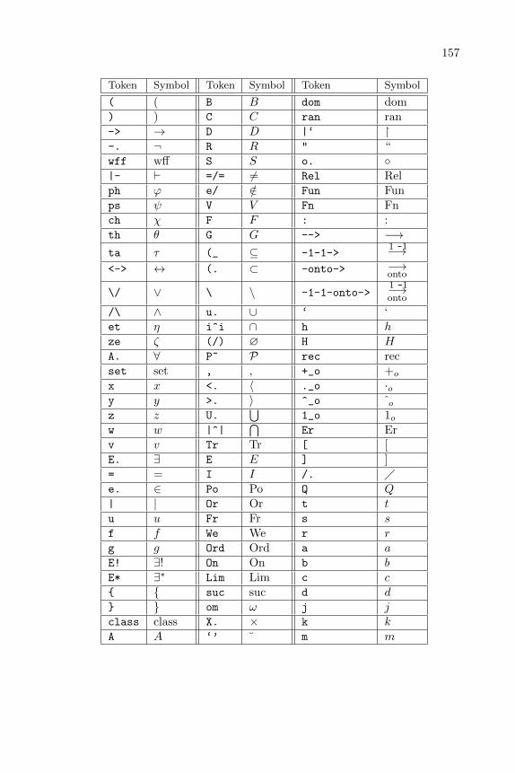
157
Token Symbol Token Symbol Token Symbol
( ( B B dom dom) ) C C ran ran-> → D D |‘ �-. ¬ R R " “wff wff S S o. ◦|- ` =/= 6= Rel Relph ϕ e/ /∈ Fun Funps ψ V V Fn Fnch χ F F : :th θ G G --> −→ta τ (_ ⊆ -1-1->
1 -1−→<-> ↔ (. ⊂ -onto-> −→
onto
\/ ∨ \ \ -1-1-onto->1 -1−→onto
/\ ∧ u. ∪ ‘ ‘et η i^i ∩ h hze ζ (/) ∅ H HA. ∀ P~ P rec recset set , , +_o +o
x x <. 〈 ._o ·oy y >. 〉 ^_o o
z z U.⋃
1_o 1ow w |^|
⋂Er Er
v v Tr Tr [ [E. ∃ E E ] ]= = I I /. �e. ∈ Po Po Q Q| | Or Or t tu u Fr Fr s sf f We We r rg g Ord Ord a aE! ∃! On On b bE* ∃∗ Lim Lim c c{ { suc suc d d} } om ω j jclass class X. × k kA A ‘’ ˘ m m

158 APPENDIX A. MATH SYMBOL TOKENS FOR SET THEORY
Token Symbol Token Symbol Token Symbol
n n +R +Rq q .R ·RJ J <R <RK K CC CL L RR RM M 0 0N N 1 1W W i iX X + +Y Y - −Z Z x. ·N. N < <+N +N / /.N ·N > ><N <N <_ ≤+pQ +pQ >_ ≥.pQ ·pQ NN N~Q ∼Q ZZ ZQ. Q QQ Q1Q 1Q 2 2+Q +Q 3 3.Q ·Q 4 4*Q ∗Q 5 5<Q <Q 6 6P. P 7 71P 1P 8 8+P +P 9 9.P ·P<P <P+pR +pR.pR .pR~R ∼RR. R0R 0R1R 1R-1R −1R

Appendix B
Compressed Proofs
The proofs in the set.mm set theory database are stored in compressedformat for efficiency. Normally you needn’t concern yourself with the com-pressed format, since you can display it with the usual proof display tools inthe Metamath program (show proof. . . ) or convert it to the normal RPNproof format described in the Section 4.3 (with save proof label /normal).However for sake of completeness we describe the format here and show howit maps to the normal RPN proof format.
A compressed proof, located between $= and $. keywords, consists ofa left parenthesis, a sequence of statement labels, a right parenthesis, anda sequence of upper-case letters A through Z (with optional white spacebetween them). White space must surround the parentheses and the labels.The left parenthesis tells Metamath that a compressed proof follows. (Anormal RPN proof consists of just a sequence of labels, and a parenthesis isnot a legal character in a label.)
The sequence of upper-case letters corresponds to a sequence of integerswith the following mapping. Each integer corresponds to a proof step asdescribed later.
A = 1B = 2
. . .T = 20UA = 21UB = 22
. . .UT = 40VA = 41VB = 42
. . .YT = 120
159
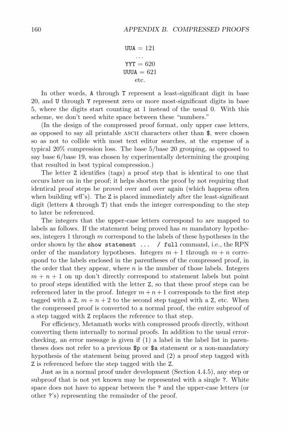
160 APPENDIX B. COMPRESSED PROOFS
UUA = 121. . .
YYT = 620UUUA = 621
etc.
In other words, A through T represent a least-significant digit in base20, and U through Y represent zero or more most-significant digits in base5, where the digits start counting at 1 instead of the usual 0. With thisscheme, we don’t need white space between these “numbers.”
(In the design of the compressed proof format, only upper case letters,as opposed to say all printable ascii characters other than $, were chosenso as not to collide with most text editor searches, at the expense of atypical 20% compression loss. The base 5/base 20 grouping, as opposed tosay base 6/base 19, was chosen by experimentally determining the groupingthat resulted in best typical compression.)
The letter Z identifies (tags) a proof step that is identical to one thatoccurs later on in the proof; it helps shorten the proof by not requiring thatidentical proof steps be proved over and over again (which happens oftenwhen building wff’s). The Z is placed immediately after the least-significantdigit (letters A through T) that ends the integer corresponding to the stepto later be referenced.
The integers that the upper-case letters correspond to are mapped tolabels as follows. If the statement being proved has m mandatory hypothe-ses, integers 1 through m correspond to the labels of these hypotheses in theorder shown by the show statement ... / full command, i.e., the RPNorder of the mandatory hypotheses. Integers m + 1 through m + n corre-spond to the labels enclosed in the parentheses of the compressed proof, inthe order that they appear, where n is the number of those labels. Integersm + n + 1 on up don’t directly correspond to statement labels but pointto proof steps identified with the letter Z, so that these proof steps can bereferenced later in the proof. Integer m+n+ 1 corresponds to the first steptagged with a Z, m + n + 2 to the second step tagged with a Z, etc. Whenthe compressed proof is converted to a normal proof, the entire subproof ofa step tagged with Z replaces the reference to that step.
For efficiency, Metamath works with compressed proofs directly, withoutconverting them internally to normal proofs. In addition to the usual error-checking, an error message is given if (1) a label in the label list in paren-theses does not refer to a previous $p or $a statement or a non-mandatoryhypothesis of the statement being proved and (2) a proof step tagged withZ is referenced before the step tagged with the Z.
Just as in a normal proof under development (Section 4.4.5), any step orsubproof that is not yet known may be represented with a single ?. Whitespace does not have to appear between the ? and the upper-case letters (orother ?’s) representing the remainder of the proof.

Appendix C
Metamath’s FormalSystem
C.1 Introduction
Perfection is when there is no longer anything more to take away.
Antoine de Saint-Exupery1
This appendix describes the theory behind the Metamath language inan abstract way intended for mathematicians. Specifically, we construct twoset-theoretical objects: a “formal system” (roughly, a set of syntax rules,axioms, and logical rules) and its “universe” (roughly, the set of theoremsderivable in the formal system). The Metamath computer language providesus with a way to describe specific formal systems and, with the aid of a proofprovided by the user, to verify that given theorems belong to their universes.
To understand this appendix, you need a basic knowledge of informalset theory. It should be sufficient to understand, for example, Ch. 1 ofMunkres’ Topology [41] or the introductory set theory chapter in many text-books that introduce abstract mathematics. (Note that there are minornotational differences among authors; e.g. Munkres uses ⊂ instead of our ⊆for “subset.” We use “included in” to mean “a subset of,” and “belongs to”or “is contained in” to mean “is an element of.”) What we call a “formal”description here, unlike earlier, is actually an informal description in theordinary language of mathematicians. However we provide sufficient detailso that a mathematician could easily formalize it, even in the language ofMetamath itself if desired. To understand the logic examples at the end ofthis appendix, familiarity with an introductory book on mathematical logicwould be helpful.
1[9, p. 3-25]
161

162 APPENDIX C. METAMATH’S FORMAL SYSTEM
C.2 The Formal Description
C.2.1 Preliminaries2
By ω we denote the set of all natural numbers (non-negative integers). Eachnatural number n is identified with the set of all smaller numbers: n ={m|m < n}. The formula m < n is thus equivalent to the condition: m ∈ nand m,n ∈ ω. In particular, 0 is the number zero and at the same time theempty set ∅, 1 = {0}, 2 = {0, 1}, etc. BA denotes the set of all functionson B to A (i.e. with domain B and range included in A). The members ofωA are what are called simple infinite sequences, with all terms in A. Incase n ∈ ω, the members of nA are referred to as finite n-termed sequences,again with terms in A. The consecutive terms (function values) of a finite orinfinite sequence f are denoted by f0, f1, . . . , fn, . . .. Every finite sequencef ∈
⋃n∈ω
nA uniquely determines the number n such that f ∈ nA; n iscalled the length of f and is denoted by |f |. 〈a〉 is the sequence f with|f | = 1 and f0 = a; 〈a, b〉 is the sequence f with |f | = 2, f0 = a, f1 = b; etc.Given two finite sequences f and g, we denote by f _ g their concatenation,i.e., the finite sequence h determined by the conditions:
|h| = |f |+ |g|;hn = fn for n < |f |;
h|f |+n = gn for n < |g|.
C.2.2 Constants, Variables, and Expressions
A formal system has a set of symbols denoted by SM. A precise set-theo-retical definition of this set is unimportant; a symbol could be considereda primitive or atomic element if we wish. We assume this set is dividedinto two disjoint subsets: a set CN of constants and a set VR of variables.CN and VR are each assumed to consist of countably many symbols whichmay be arranged in finite or simple infinite sequences c0, c1, . . . and v0, v1, . . .respectively, without repeating terms. We will represent arbitrary symbolsby metavariables α, β, etc.
Comment. The variables v0, v1, . . . of our formal system correspondto what are usually considered “metavariables” in descriptions of specificformal systems in the literature. Typically, when describing a specific formalsystem a book will postulate a set of primitive objects called variables, thenproceed to describe their properties using metavariables that range overthem, never mentioning again the actual variables themselves. Our formalsystem does not mention these primitive variable objects at all but dealsdirectly with metavariables, as its primitive objects, from the start. Thisis a subtle but key distinction you should keep in mind, and it makes ourdefinition of “formal system” somewhat different from that typically foundin the literature. (So, the α, β, etc. above are actually “metametavariables”when used to represent v0, v1, . . ..)
2This section is taken mostly verbatim from Tarski [61, p. 63].

C.2. THE FORMAL DESCRIPTION 163
Finite sequences all terms of which are symbols are called expressions.EX is the set of all expressions; thus
EX =⋃n∈ω
nSM.
A constant-prefixed expression is a an expression of non-zero length whosefirst term is a constant. We denote the set of all constant-prefixed expres-sions by EXC = {e ∈ EX|(|e| > 0 ∧ e0 ∈ CN)}.
A constant-variable pair is an expression of length 2 whose first term isa constant and whose second term is a variable. We denote the set of allconstant-variable pairs by EX2 = {e ∈ EXC |(|e| = 2 ∧ e1 ∈ VR)}.
Relationship to Metamath. In general, the set SM corresponds to theset of declared math symbols in a Metamath database, the set CN to thosedeclared with $c statements, and the set VR to those declared with $v
statements. Of course a Metamath database can only have a finite numberof math symbols, whereas formal systems in general can have an infinitenumber, although the number of Metamath math symbols available is inprinciple unlimited.
The set EXC corresponds to the set of permissible expressions for $e,$a, and $p statements. The set EX2 corresponds to the set of permissibleexpressions for $f statements.
We denote by V(e) the set of all variables in an expression e ∈ EX, i.e.the set of all α ∈ VR such that α = en for some n < |e|. We also denote(with abuse of notation) by V(E) the set of all variables in a collection ofexpressions E ⊆ EX, i.e.
⋃e∈E V(e).
C.2.3 Substitution
Given a function F from VR to EX, we denote by σF or just σ the functionfrom EX to EX defined recursively for nonempty sequences by
σ(< α >) = F (α) for α ∈ VR;
σ(< α >) =< α > for α 6∈ VR;
σ(g _ h) = σ(g) _ σ(h) for g, h ∈ EX.
We also define σ(∅) = ∅. We call σ a simultaneous substitution (or justsubstitution) with substitution map F .
We also denote (with abuse of notation) by σ(E) a substitution on acollection of expressions E ⊆ EX, i.e. the set {σ(e)|e ∈ E}. The collectionσ(E) may of course contain fewer expressions than E because duplicateexpressions could result from the substitution.
C.2.4 Statements
We denote by DV the set of all unordered pairs {α, β} ⊆ VR such thatα 6= β. DV stands for “distinct variables.”
164 APPENDIX C. METAMATH’S FORMAL SYSTEM
A pre-statement is a quadruple 〈D,T,H,A〉 such that D ⊆ DV, T ⊆EX2, H ⊆ EXC and H is finite, A ∈ EXC , V(H ∪ {A}) ⊆ V(T ), and∀e, f ∈ T V(e) 6= V(f) (or equivalently, e1 6= f1) whenever e 6= f . Theterms of the quadruple are called distinct-variable restrictions, variable-typehypotheses, logical hypotheses, and the assertion respectively. We denote byTM (mandatory variable-type hypotheses) the subset of T such that V(TM ) =V(H ∪ {A}). We denote by DM = {{α, β} ∈ D|{α, β} ⊆ V(TM )} themandatory distinct-variable restrictions of the pre-statement. The set ofmandatory hypotheses is TM ∪ H. We call the quadruple 〈DM , TM , H,A〉the reduct of the pre-statement 〈D,T,H,A〉.
A statement is the reduct of some pre-statement. A statement is thereforea special kind of pre-statement; in particular, a statement is the reduct ofitself.
Comment. T is a set of expressions, each of length 2, that associate a setof constants (“variable types”) with a set of variables. The condition V(H∪{A}) ⊆ V(T ) means that each variable occurring in a statement’s logicalhypotheses or assertion must have an associated variable-type hypothesisor “type declaration,” in analogy to a computer programming language,where a variable must be declared to be say, a string or an integer. Therequirement that ∀e, f ∈ T e1 6= f1 for e 6= f means that each variable mustbe associated with a unique constant designating its variable type; e.g., avariable might be a “wff” or a “set” but not both.
Distinct-variable restrictions are used to specify what variable substi-tutions are permissible to make for the statement to remain valid. Forexample, in the theorem scheme of set theory ¬∀xx = y we may not sub-stitute the same variable for both x and y. On the other hand, the theoremscheme x = y → y = x does not require that x and y be distinct, so we donot require a distinct-variable restriction, although having one would causeno harm other than making the scheme less general.
A mandatory variable-type hypothesis is one whose variable exists ina logical hypothesis or the assertion. A provable pre-statement (definedbelow) may require non-mandatory variable-type hypotheses that effectivelyintroduce “dummy” variables for use in its proof. Any number of dummyvariables might be required by a specific proof; indeed, it has been shown byH. Andreka [43] that there is no finite upper bound to the number of dummyvariables needed to prove an arbitrary theorem in first-order logic (withequality) having a fixed number n > 2 of individual variables. (See also theComment on p. 105.) For this reason we do not set a finite size bound on thecollections D and T , although in an actual application (Metamath database)these will of course be finite, increased to whatever size is necessary as moreproofs are added.
Relationship to Metamath. A pre-statement of a formal system corre-sponds to an extended frame in a Metamath database (Section 4.2.7). Thecollections D, T , and H correspond respectively to the $d, $f, and $e state-ment collections in an extended frame. The expression A corresponds to the$a (or $p) statement in an extended frame.
A statement of a formal system corresponds to a frame in a Metamathdatabase.

C.2. THE FORMAL DESCRIPTION 165
C.2.5 Formal Systems
A formal system is a triple 〈CN,VR,Γ〉 where Γ is a set of statements. Themembers of Γ are called axiomatic statements. Sometimes we will refer to aformal system by just Γ when CN and VR are understood.
Given a formal system Γ, the closure3 of a pre-statement 〈D,T,H,A〉 isthe smallest set C of expressions such that:
1. T ∪H ⊆ C; and
2. If for some axiomatic statement 〈D′M , T ′M , H ′, A′〉 ∈ Γ and for somesubstitution σ we have
a. σ(T ′M ∪H ′) ⊆ C; and
b. for all {α, β} ∈ D′M , for all γ ∈ V(σ(〈α〉)), and for all δ ∈V(σ(〈β〉)), we have {γ, δ} ∈ D;
then σ(A′) ∈ C.
A pre-statement 〈D,T,H,A〉 is provable if A ∈ C i.e. if its assertion belongsto its closure. A statement is provable if it is the reduct of a provablepre-statement. The universe of a formal system is the collection of all ofits provable statements. Note that the set of axiomatic statements Γ in aformal system is a subset of its universe.
Comment. The first condition in the definition of closure simply saysthat the hypotheses of the pre-statement are in its closure.
Condition 2(a) says that a substitution exists that makes the mandatoryhypotheses of an axiomatic statement exactly match some members of theclosure. This is what we explicitly demonstrate in a Metamath languageproof.
Condition 2(b) describes how distinct-variable restrictions in the ax-iomatic statement must be met. It means that after a substitution for twovariables that must be distinct, the resulting two expressions must eithercontain no variables, or if they do, they may not have variables in common,and each pair of any variables they do have, with one variable from eachexpression, must be specified as distinct in the original statement.
Relationship to Metamath. Axiomatic statements and provable state-ments in a formal system correspond to the frames for $a and $p statementsrespectively in a Metamath database. The set of axiomatic statements area subset of the set of provable statements in a formal system, although in aMetamath database a $a statement is distinguished by not having a proof.A Metamath language proof for a $p statement tells the computer how toexplicitly construct a series of members of the closure ultimately leadingto a demonstration that the assertion being proved is in the closure. Theactual closure typically contains an infinite number of expressions. A formalsystem itself does not have an explicit object called a “proof” but ratherthe existence of a proof is implied indirectly by membership of an assertionin a provable statement’s closure. We do this to make the formal systemeasier to describe in the language of set theory.
3This definition of closure incorporates a simplification due to Josh Purinton.

166 APPENDIX C. METAMATH’S FORMAL SYSTEM
We also note that once established as provable, a statement may beconsidered to acquire the same status as an axiomatic statement, becauseif the set of axiomatic statements is extended with a provable statement,the universe of the formal system remains unchanged (provided that VRis infinite). In practice, this means we can build a hierarchy of provablestatements to more efficiently establish additional provable statements. Thisis what we do in Metamath when we allow proofs to reference previous $p
statements as well as previous $a statements.
C.3 Examples of Formal Systems
Relationship to Metamath. The examples in this section, except Exam-ple 2, are for the most part exact equivalents of the development in the settheory database set.mm. You may want to compare Examples 1, 3, and 5to Section 3.3, Example 4 to Sections 3.4.1 and 3.4.2, and Example 6 toSection 3.4.3.
C.3.1 Example 1—Propositional Calculus
Classical propositional calculus can be described by the following formalsystem. We assume the set of variables is infinite. Rather than denoting theconstants and variables by c0, c1, . . . and v0, v1, . . ., for readability we willinstead use more conventional symbols, with the understanding of coursethat they denote distinct primitive objects. Also for readability we mayomit commas between successive terms of a sequence; thus 〈wff ϕ〉 denotes〈wff, ϕ〉.
Let
CN = {wff,`,→,¬, (, )}
VR = {ϕ,ψ, χ, . . .}
T = {〈wff ϕ〉, 〈wff ψ〉, 〈wff χ〉, . . .}, i.e. those expressions of length 2whose first member is wff and whose second member belongs to VR.4
Then Γ consists of the axiomatic statements that are the reducts offollowing pre-statements:
〈∅, T,∅, 〈wff (ϕ→ ψ)〉〉〈∅, T,∅, 〈wff ¬ϕ〉〉〈∅, T,∅, 〈` (ϕ→ (ψ → ϕ))〉〉〈∅, T,∅, 〈` ((ϕ→ (ψ → χ))→ ((ϕ→ ψ)→ (ϕ→ χ)))〉〉
4For convenience we let T be an infinite set; the definition of a statement permitsthis in principle. Since a Metamath source file has a finite size, in practice we mustof course use appropriate finite subsets of this T , specifically ones containing at leastthe mandatory variable-type hypotheses. Similarly, in the source file we introduce newvariables as required, with the understanding that a potentially infinite number of themare available.

C.3. EXAMPLES OF FORMAL SYSTEMS 167
〈∅, T,∅, 〈` ((¬ϕ→ ¬ψ)→ (ψ → ϕ))〉〉〈∅, T, {〈` (ϕ→ ψ)〉, 〈` ϕ〉}, 〈` ψ〉〉
(For example, the reduct of 〈∅, T,∅, 〈wff (ϕ→ ψ)〉〉 is
〈∅, {〈wff ϕ〉, 〈wff ψ〉},∅, 〈wff (ϕ→ ψ)〉〉,
which is the first axiomatic statement.)We call the members of VR wff variables or (in the context of first-order
logic which we will describe shortly) wff metavariables. Note that the sym-bols φ, ψ, etc. denote actual specific members of VR; they are not metavari-ables of our expository language (which we denote with α, β, etc.) but areinstead (meta)constant symbols (members of SM) from the point of viewof our expository language. The equivalent system of propositional calculusdescribed in [61] also uses the symbols φ, ψ, etc. to denote wff metavariables,but in [61] unlike here those are metavariables of the expository languageand not primitive symbols of the formal system.
The first two statements define wffs: if ϕ and ψ are wffs, so is (ϕ→ ψ); ifϕ is a wff, so is ¬ϕ. The next three are the axioms of propositional calculus:if ϕ and ψ are wffs, then ` (ϕ → (ψ → ϕ)) is an (axiomatic) theorem; etc.The last is the rule of modus ponens: if ϕ and ψ are wffs, and ` (ϕ → ψ)and ` ϕ are theorems, then ` ψ is a theorem.
The correspondence to ordinary propositional calculus is as follows. Weconsider only provable statements of the form 〈∅, T,∅, A〉 with T definedas above. The first term of the assertion A of any such statement is either“wff” or “`”. A statement for which first term is “wff” is a wff of proposi-tional calculus, and one where the first term is “`” is a theorem (scheme) ofpropositional calculus.
The universe of this formal system also contains many other provablestatements. Those with distinct-variable restrictions are irrelevant becausepropositional calculus has no constraints on substitutions. Those that havelogical hypotheses we call inferences when the logical hypotheses are of theform 〈`〉 _ w where w is a wff (with the leading constant term “wff”removed). Inferences (other than the modus ponens rule) are not a properpart of propositional calculus but are convenient to use when building ahierarchy of provable statements. A provable statement with a nonsensehypothesis such as 〈→,`,¬〉, and this same expression as its assertion, weconsider irrelevant; no use can be made of it in proving theorems, since thereis no way to eliminate the nonsense hypothesis.
Comment. Our use of parentheses in the definition of a wff illustrateshow axiomatic statements should be carefully stated in a way that ties inunambiguously with the substitutions allowed by the formal system. Thereare many ways we could have defined wffs—for example, Polish prefix no-tation would have allowed us to omit parentheses entirely, at the expense ofreadability—but we must define them in a way that is unambiguous. Forexample, if we had omitted parentheses from the definition of (ϕ→ ψ), thewff ¬ϕ → ψ could be interpreted as either ¬(ϕ → ψ) or (¬ϕ → ψ) and

168 APPENDIX C. METAMATH’S FORMAL SYSTEM
would have allowed us to prove nonsense. Note that there is no concept ofoperator binding precedence built into our formal system.
C.3.2 Example 2—Predicate Calculus with Equality
Here we extend Example 1 to include predicate calculus with equality, illus-trating the use of distinct-variable restrictions. This system is the same asTarski’s system S2 in [61] (except that the axioms of propositional calculusare different but equivalent, and a redundant axiom is omitted). We extendCN with the constants {var,∀,=}. We extend VR with an infinite set ofindividual metavariables {x, y, z, . . .} and denote this subset Vr.
We also join to CN a possibly infinite set Pr of predicates {R,S, . . .}. Weassociate with Pr a function rnk from Pr to ω, and for α ∈ Pr we call rnk(α)the rank of the predicate α, which is simply the number of “arguments” thatthe predicate has. (Most applications of predicate calculus will have a finitenumber of predicates; for example, set theory has the single two-argument orbinary predicate ∈, which is usually written with its arguments surroundingthe predicate symbol rather than with the prefix notation we will use forthe general case.) As a device to facilitate our discussion, we will let Vs beany fixed one-to-one function from ω to Vr; thus Vs is any simple infinitesequence of individual metavariables with no repeating terms.
In this example we will not include the function symbols that are of-ten part of formalizations of predicate calculus. Using metalogical argu-ments that are beyond the scope of our discussion, it can be shown that ourformalization is equivalent when functions are introduced via appropriatedefinitions.
We extend the set T defined in Example 1 with the expressions {〈var x〉,〈var y〉, 〈var z〉, . . .}. We extend the Γ above with the axiomatic statementsthat are the reducts of the following pre-statements:
〈∅, T,∅, 〈wff ∀xϕ〉〉〈∅, T,∅, 〈wff x = y〉〉〈∅, T, {〈` ϕ〉}, 〈` ∀xϕ〉〉〈∅, T,∅, 〈` ((∀x(ϕ→ ψ)→ (∀xϕ→ ∀xψ))〉〉〈{{x, ϕ}}, T,∅, 〈` (ϕ→ ∀xϕ)〉〉〈{{x, y}}, T,∅, 〈` ¬∀x¬x = y〉〉〈∅, T,∅, 〈` (x = z → (x = y → z = y))〉〉〈∅, T,∅, 〈` (y = z → (x = y → x = z))〉〉
These are the axioms not involving predicate symbols. The first two state-ments extend the definition of a wff. The third is the rule of generalization.The fifth states, in effect, “For a wff ϕ and variable x, ` (ϕ → ∀xϕ), pro-vided that x does not occur in ϕ.” The sixth states “For a variables x and

C.3. EXAMPLES OF FORMAL SYSTEMS 169
y, ` ¬∀x¬x = y, provided that x and y are distinct.” (This proviso is notnecessary but was included by Tarski to weaken the axiom and still showthat the system is logically complete.)
Finally, for each predicate symbol α ∈ Pr, we add to Γ the an axiomaticstatement, extending the definition of wff, that is the reduct of the followingpre-statement:
〈∅, T,∅, 〈wff, α〉 _ Vs � rnk(α)〉
and for each α ∈ Pr and each n < rnk(α) we add to Γ an equality axiomthat is the reduct of the following pre-statement:
〈∅, T,∅, 〈`, (,Vsn,=,Vsrnk(α),→, (, α〉_ Vs � rnk(α)
_ 〈→, α〉_ Vs � n _ 〈Vsrnk(α)〉
_ Vs � (rnk(α) \ (n+ 1)) _ 〈), )〉〉
where � denotes function domain restriction and \ denotes set difference.Recall that a subscript on Vs denotes one of its terms. (In the above twoaxiom sets commas are placed between successive terms of sequences toprevent ambiguity, and if you examine them with care you will be ableto distinguish those parentheses that denote constant symbols from those ofour expository language that delimit function arguments. Although it mighthave been better to use boldface for our primitive symbols, unfortunatelyboldface was not available for all characters on the LATEX system used totypeset this text.) These seemingly forbidding axioms can be understood byanalogy to concatenation of substrings in a computer language. They areactually relatively simple for each specific case and will become clearer bylooking at the special case of a binary predicate α = R where rnk(R) = 2.Letting Vs be the sequence 〈x, y, z, . . .〉, the axioms we would add to Γ forthis case would be the wff extension and two equality axioms that are thereducts of the pre-statements:
〈∅, T,∅, 〈wff Rxy〉〉〈∅, T,∅, 〈` (x = z → (Rxy → Rzy))〉〉〈∅, T,∅, 〈` (y = z → (Rxy → Rxz))〉〉
Study these carefully to see how the general axioms above evaluate to them.In practice, typically only a few special cases such as this would be needed,and in any case the Metamath language will only permit us to describe afinite number of predicates, as opposed to the infinite number permittedby the formal system. (If an infinite number should be needed for somereason, we could not define the formal system directly in the Metamathlanguage but could instead define it metalogically under set theory as we doin this appendix, and only the underlying set theory, with its single binarypredicate, would be defined directly in the Metamath language.)
170 APPENDIX C. METAMATH’S FORMAL SYSTEM
Comment. As we noted earlier, the specific variables denoted by thesymbols x, y, z, . . . ∈ Vr ⊆ VR ⊆ SM in Example 2 are not the actual vari-ables of ordinary predicate calculus but should be thought of as metavari-ables ranging over them. For example, a distinct-variable restriction wouldbe meaningless for actual variables of ordinary predicate calculus since twodifferent actual variables are by definition distinct. And when we talk aboutan arbitrary representative α ∈ Vr, α is a metavariable (in our expositorylanguage) that ranges over metavariables (which are primitives of our for-mal system) each of which ranges over the actual individual variables ofpredicate calculus (which are never mentioned in our formal system).
The constant called “var” above is called set in the set.mm database file,but it means the same thing. I felt that “var” is a more meaningful name inthe context of predicate calculus, whose use is not limited to set theory. Forconsistency we stick with the name “var” throughout this Appendix, evenafter set theory is introduced.
C.3.3 Free Variables and Proper Substitution
In the system of Example 2, there are no primitive notions of free vari-able and proper substitution. Tarski [61] shows that this system is logicallyequivalent to the more typical textbook systems that do have these primi-tive notions, if we introduce these notions with appropriate definitions andmetalogic. We could also define axioms for such systems directly, althoughthe recursive definitions of free variable and proper substitution would bemessy and awkward to work with. Instead, we mention two devices thatcan be used in practice to mimic these notions. (1) Instead of introducingspecial notation to express (as a logical hypothesis) “where x is not free inϕ” we can use the logical hypothesis ` (ϕ → ∀xϕ).5 (2) It can be shownthat the wff ((x = y → ϕ) ∧ ∃x(x = y ∧ ϕ)) (with the usual definitions of ∧and ∃; see Example 4 below) is logically equivalent to “the wff that resultsfrom proper substitution of y for x in ϕ.” This works whether or not x andy are distinct.
C.3.4 Metalogical Completeness
In the system of Example 2, the following are provable pre-statements (andtheir reducts are provable statements):
〈{{x, y}}, T,∅, 〈` ¬∀x¬x = y〉〉〈∅, T,∅, 〈` ¬∀x¬x = x〉〉
whereas the following pre-statement is not to my knowledge provable (butin any case we will pretend it’s not for sake of illustration) :
〈∅, T,∅, 〈` ¬∀x¬x = y〉〉5This is a slightly weaker requirement than “where x is not free in ϕ.” If we let ϕ
be x = x, we have the theorem (x = x → ∀xx = x) which satisfies the hypothesis, eventhough x is free in x = x . In a case like this we say that x is effectively not free in x = x,since x = x is logically equivalent to ∀xx = x in which x is bound.

C.3. EXAMPLES OF FORMAL SYSTEMS 171
In other words, we can prove “¬∀x¬x = y where x and y are distinct” andseparately prove “¬∀x¬x = x”, but we can’t prove the combined generalcase “¬∀x¬x = y” that has no proviso. Now this does not compromise logi-cal completeness, because the variables are really metavariables and the twoprovable cases together cover all possible cases. The third case can be con-sidered a metatheorem whose direct proof, using the system of Example 2,lies outside the capability of the formal system.
Also, in the system of Example 2 the following pre-statement is not tomy knowledge provable (again, a conjecture that we will pretend to be thecase):
〈∅, T,∅, 〈` (∀xϕ→ ϕ)〉〉
Instead, we can only prove specific cases of ϕ involving individual metavari-ables, and by induction on formula length, prove as a metatheorem outsideof our formal system the general statement above. The details of this proofare found in [25].
There does, however, exist a system of predicate calculus in which allsuch “simple metatheorems” as those above can be proved directly, and wepresent it in Example 3. A simple metatheorem is any statement of theformal system of Example 2 where all distinct variable restrictions consistof either two individual metavariables or an individual metavariable anda wff metavariable, and which is provable by combining cases outside thesystem as above. A system is metalogically complete if all of its simplemetatheorems are (directly) provable statements. The precise definition of“simple metatheorem” and the proof of the “metalogical completeness” ofExample 3 is found in Remark 9.6 and Theorem 9.7 of [34].
C.3.5 Example 3—Metalogically Complete PredicateCalculus with Equality
For simplicity we will assume there is one binary predicate R; this systemsuffices for set theory, where the R is of course the ∈ predicate. We label theaxioms as they appear in [34]. This system is logically equivalent to that ofExample 2 (when the latter is restricted to this single binary predicate) butis also metalogically complete.
Let
CN = {wff, var,`,→,¬, (, ),∀,=, R}.
VR = {ϕ,ψ, χ, . . .} ∪ {x, y, z, . . .}.
T = {〈wff ϕ〉, 〈wff ψ〉, 〈wff χ〉, . . .} ∪ {〈var x〉, 〈var y〉, 〈var z〉, . . .}.Then Γ consists of the reducts of the following pre-statements:
〈∅, T,∅, 〈wff (ϕ→ ψ)〉〉
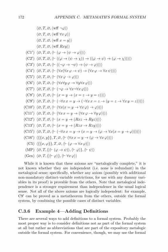
172 APPENDIX C. METAMATH’S FORMAL SYSTEM
〈∅, T,∅, 〈wff ¬ϕ〉〉〈∅, T,∅, 〈wff ∀xϕ〉〉〈∅, T,∅, 〈wff x = y〉〉〈∅, T,∅, 〈wff Rxy〉〉
(C1′) 〈∅, T,∅, 〈` (ϕ→ (ψ → ϕ))〉〉(C2′) 〈∅, T,∅, 〈` ((ϕ→ (ψ → χ))→ ((ϕ→ ψ)→ (ϕ→ χ)))〉〉(C3′) 〈∅, T,∅, 〈` ((¬ϕ→ ¬ψ)→ (ψ → ϕ))〉〉(C4′) 〈∅, T,∅, 〈` (∀x(∀xϕ→ ψ)→ (∀xϕ→ ∀xψ))〉〉(C5′) 〈∅, T,∅, 〈` (∀xϕ→ ϕ)〉〉(C6′) 〈∅, T,∅, 〈` (∀x∀y ϕ→ ∀y∀xϕ)〉〉(C7′) 〈∅, T,∅, 〈` (¬ϕ→ ∀x¬∀xϕ)〉〉(C8′) 〈∅, T,∅, 〈` (x = y → (x = z → y = z))〉〉(C9′) 〈∅, T,∅, 〈` (¬∀xx = y → (¬∀xx = z → (y = z → ∀x y = z)))〉〉
(C10′) 〈∅, T,∅, 〈` (∀x(x = y → ∀xϕ)→ ϕ))〉〉(C11′) 〈∅, T,∅, 〈` (∀xx = y → (∀xϕ→ ∀y ϕ))〉〉(C12′) 〈∅, T,∅, 〈` (x = y → (Rxz → Ryz))〉〉(C13′) 〈∅, T,∅, 〈` (x = y → (Rzx→ Rzy))〉〉(C15′) 〈∅, T,∅, 〈` (¬∀xx = y → (x = y → (ϕ→ ∀x(x = y → ϕ))))〉〉(C16′) 〈{{x, y}}, T,∅, 〈` (∀xx = y → (ϕ→ ∀xϕ))〉〉
(C5) 〈{{x, ϕ}}, T,∅, 〈` (ϕ→ ∀xϕ)〉〉(MP) 〈∅, T, {〈` (ϕ→ ψ)〉, 〈` ϕ〉}, 〈` ψ〉〉(Gen) 〈∅, T, {〈` ϕ〉}, 〈` ∀xϕ〉〉
While it is known that these axioms are “metalogically complete,” it isnot known whether they are independent (i.e. none is redundant) in themetalogical sense; specifically, whether any axiom (possibly with additionalnon-mandatory distinct-variable restrictions, for use with any dummy vari-ables in its proof) is provable from the others. Note that metalogical inde-pendence is a stronger requirement than independence in the usual logicalsense. Not all of the above axioms are logically independent: for example,C9′ can be proved as a metatheorem from the others, outside the formalsystem, by combining the possible cases of distinct variables.
C.3.6 Example 4—Adding Definitions
There are several ways to add definitions to a formal system. Probably themost proper way is to consider definitions not as part of the formal systemat all but rather as abbreviations that are part of the expository metalogicoutside the formal system. For convenience, though, we may use the formal

C.3. EXAMPLES OF FORMAL SYSTEMS 173
system itself to incorporate definitions, adding them as axiomatic exten-sions to the system. This could be done by adding a constant representingthe concept “is defined as” along with axioms for it. But there is a nicerway, at least in this writer’s opinion, that introduces definitions as directextensions to the language rather than as extralogical primitive notions. Weintroduce additional logical connectives and provide axioms for them. Forsystems of logic such as Examples 1 through 3, the additional axioms mustbe conservative in the sense that no wff of the original system that was not atheorem (when the initial term “wff” is replaced by “`” of course) becomesa theorem of the extended system. In this example we extend Example 3(or 2) with standard abbreviations of logic.
We extend CN of Example 3 with new constants {↔,∧,∨,∃}, corre-sponding to logical equivalence, conjunction, disjunction, and the existentialquantifier. We extend Γ with the axiomatic statements that are the reductsof the following pre-statements:
〈∅, T,∅, 〈wff (ϕ↔ ψ)〉〉〈∅, T,∅, 〈wff (ϕ ∨ ψ)〉〉〈∅, T,∅, 〈wff (ϕ ∧ ψ)〉〉〈∅, T,∅, 〈wff ∃xϕ〉〉〈∅, T,∅, 〈` ((ϕ↔ ψ)→ (ϕ→ ψ))〉〉〈∅, T,∅, 〈` ((ϕ↔ ψ)→ (ψ → ϕ))〉〉〈∅, T,∅, 〈` ((ϕ→ ψ)→ ((ψ → ϕ)→ (ϕ↔ ψ)))〉〉〈∅, T,∅, 〈` ((ϕ ∧ ψ)↔ ¬(ϕ→ ¬ψ))〉〉〈∅, T,∅, 〈` ((ϕ ∨ ψ)↔ (¬ϕ→ ψ))〉〉〈∅, T,∅, 〈` (∃xϕ↔ ¬∀x¬ϕ)〉〉
The first three logical axioms (statements containing “`”) introduce andeffectively define logical equivalence, “↔”. The last three use “↔” to effec-tively mean “is defined as.”
C.3.7 Example 5—ZFC Set Theory
Here we add to the system of Example 4 the axioms of Zermelo-Fraenkelset theory with Choice. For convenience we make use of the definitions inExample 4.
In the CN of Example 4 (which extends Example 3), we replace thesymbol R with the symbol ∈. We remove from Γ of Example 4 the threeaxiomatic statements containing R and replace them with the reducts of thefollowing:
〈∅, T,∅, 〈wff x ∈ y〉〉〈∅, T,∅, 〈` (x = y → (x ∈ z → y ∈ z))〉〉

174 APPENDIX C. METAMATH’S FORMAL SYSTEM
〈∅, T,∅, 〈` (x = y → (z ∈ x→ z ∈ y))〉〉
Letting D = {{α, β} ∈ DV |α, β ∈ Vr} (in other words all individual vari-ables must be distinct), we extend Γ with the ZFC axioms, called Exten-sionality, Replacement, Union, Power Set, Regularity, Infinity, and Choice,that are the reducts of:
Ext 〈D,T,∅, 〈` (∀x(x ∈ y ↔ x ∈ z)→ y = z)〉〉Rep 〈D,T,∅, 〈` ∃x(∃y∀z(ϕ→ z = y)→ ∀z(z ∈ x↔ ∃x(x ∈ y ∧ ∀y ϕ)))〉〉Un 〈D,T,∅, 〈` ∃x∀y(∃x(y ∈ x ∧ x ∈ z)→ y ∈ x)〉〉
Pow 〈D,T,∅, 〈` ∃x∀y(∀x(x ∈ y → x ∈ z)→ y ∈ x)〉〉Reg 〈D,T,∅, 〈` (x ∈ y → ∃x(x ∈ y ∧ ∀z(z ∈ x→ ¬z ∈ y)))〉〉Inf 〈D,T,∅, 〈` ∃x(y ∈ x ∧ ∀y(y ∈ x→ ∃z(y ∈ z ∧ z ∈ x)))〉〉AC 〈D,T,∅, 〈` ∃x∀y∀z((y ∈ z∧z ∈ w)→ ∃w∀y(∃w((y ∈ z∧z ∈ w)∧(y ∈
w ∧ w ∈ x))↔ y = w))〉〉
C.3.8 Example 6—Class Notation in Set Theory
A powerful device that makes set theory easier (and that we have beenusing all along in our informal expository language) is class abstraction no-tation. The definitions we introduce are rigorously justified as conservativeby Takeuti and Zaring [59] or Quine [48]. The key idea is to introduce thenotation {x|—} which means “the class of all x such that —” for abstractionclasses and introduce (meta)variables that range over them. An abstractionclass may or may not be a set, depending on whether it exists (as a set). Aclass that does not exist is called a proper class.
To illustrate the use of abstraction classes we will provide some exam-ples of definitions that make use of them: the empty set, class union, andunordered pair. Many other such definitions can be found in the Metamathset theory database, set.mm.
We extend CN of Example 5 with new symbols {class, {, |, },∅,∪, , }where the inner braces and last comma are constant symbols. (As before,our dual use of some mathematical symbols for both our expository languageand as primitives of the formal system should be clear from context.)
We extend VR of Example 5 with a set of class variables {A,B,C, . . .}.We extend the T of Example 5 with {〈class A〉, 〈class B〉, 〈class C〉, . . .}.
To introduce our definitions, we add to Γ of Example 5 the axiomaticstatements that are the reducts of the following pre-statements:
〈∅, T,∅, 〈class x〉〉〈∅, T,∅, 〈class {x|ϕ}〉〉〈∅, T,∅, 〈wff A = B〉〉〈∅, T,∅, 〈wff A ∈ B〉〉

C.4. METAMATH AS A FORMAL SYSTEM 175
Ab 〈∅, T,∅, 〈` (y ∈ {x|ϕ} ↔ ((x = y → ϕ) ∧ ∃x(x = y ∧ ϕ)))〉〉Eq 〈{{x,A}, {x,B}}, T,∅, 〈` (A = B ↔ ∀x(x ∈ A↔ x ∈ B))〉〉El 〈{{x,A}, {x,B}}, T,∅, 〈` (A ∈ B ↔ ∃x(x = A ∧ x ∈ B))〉〉
Here we say that an individual variable is a class; {x|ϕ} is a class; andwe extend the definition of a wff to include class equality and membership.Axiom Ab defines membership of a variable in a class abstraction; the right-hand side can be read as “the wff that results from proper substitutionof y for x in ϕ.”6 Axioms Eq and El extend the meaning of the existingequality and membership connectives. This is potentially dangerous andrequires careful justification. For example, from Eq we can derive the Axiomof Extensionality with predicate logic alone; thus in principle we shouldinclude the Axiom of Extensionality as a logical hypothesis. However we donot bother to do this since we have already presupposed that axiom earlier.The distinct variable restrictions should be read “where x does not occurin A or B.” We typically do this when the right-hand side of a definitioninvolves an individual variable not in the expression being defined; it is doneso that the right-hand side remains independent of the particular “dummy”variable we use.
We continue to add to Γ the following definitions (i.e. the reducts of thefollowing pre-statements) for empty set, class union, and unordered pair.They should be self-explanatory. Analogous to our use of “↔” to definenew wffs in Example 4, we use “=” to define new abstraction terms, andboth may be read informally as “is defined as” in this context.
〈∅, T,∅, 〈class ∅〉〉〈∅, T,∅, 〈` ∅ = {x|¬x = x}〉〉〈∅, T,∅, 〈class (A ∪B)〉〉〈{{x,A}, {x,B}}, T,∅, 〈` (A ∪B) = {x|(x ∈ A ∨ x ∈ B)}〉〉〈∅, T,∅, 〈class {A,B}〉〉〈{{x,A}, {x,B}}, T,∅, 〈` {A,B} = {x|(x = A ∨ x = B)}〉〉
C.4 Metamath as a Formal System
This section presupposes a familiarity with the Metamath computer lan-guage.
Our theory describes formal systems and their universes. The Metamathlanguage provides a way of representing these set-theoretical objects to a
6Note that this definition makes unnecessary the introduction of a separate notationsimilar to ϕ(x|y) for proper substitution, although we may choose to do so to be con-ventional. Incidentally, ϕ(x|y) as it stands would be ambiguous in the formal systems ofour examples, since we wouldn’t know whether ¬ϕ(x|y) meant ¬(ϕ(x|y)) or (¬ϕ)(x|y).Instead, we would have to use an unambiguous variant such as (ϕx|y).

176 APPENDIX C. METAMATH’S FORMAL SYSTEM
computer. A Metamath database, being a finite set of ascii characters, canusually describe only a subset of a formal system and its universe, which aretypically infinite. However the database can contain as large a finite subsetof the formal system and its universe as we wish. (Of course a Metamathset theory database can, in principle, indirectly describe an entire infiniteformal system by formalizing the expository language in this Appendix.)
For purpose of our discussion, we assume the Metamath database is inthe simple form described on p. 111, consisting of all constant and variabledeclarations at the beginning, followed by a sequence of extended frameseach delimited by ${ and $}. Any Metamath database can be converted tothis form, as described on p. 114.
The math symbol tokens of a Metamath source file, which are declaredwith $c and $v statements, are names we assign to representatives of CN andVR. For definiteness we could assume that the first math symbol declaredas a variable corresponds to v0, the second to v1, etc., although the exactcorrespondence we choose is not important.
In the Metamath language, each $d, $f, and $e source statement inan extended frame (Section 4.2.7) corresponds respectively to a member ofthe collections D, T , and H in a formal system statement 〈DM , TM , H,A〉.The math symbol strings following these Metamath keywords correspondto a variable pair (in the case of $d) or an expression (for the other twokeywords). The math symbol string following a $a source statement cor-responds to expression A in an axiomatic statement of the formal system;the one following a $p source statement corresponds to A in a provablestatement that is not axiomatic. In other words, each extended frame in aMetamath database corresponds to a pre-statement of the formal system,and a frame corresponds to a statement of the formal system. (Don’t confusethe two meanings of “statement” here. A statement of the formal systemcorresponds to the several statements in a Metamath database that mayconstitute a frame.)
In order for the computer to verify that a formal system statement isprovable, each $p source statement is accompanied by a proof. However, theproof does not correspond to anything in the formal system but is simplya way of communicating to the computer the information needed for itsverification. The proof tells the computer how to construct specific membersof closure of the formal system pre-statement corresponding to the extendedframe of the $p statement. The final result of the construction is the memberof the closure that matches the $p statement. The abstract formal system,on the other hand, is concerned only with the existence of members of theclosure.
As mentioned on p. 166, Examples 1 and 3–6 in the previous Sectionparallel the development of logic and set theory in the Metamath databaseset.mm. You may find it instructive to compare them.
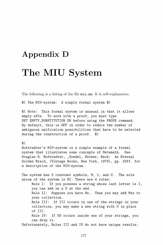
Appendix D
The MIU System
The following is a listing of the file miu.mm. It is self-explanatory.
$( The MIU-system: A simple formal system $)
$( Note: This formal system is unusual in that it allows
empty wffs. To work with a proof, you must type
SET EMPTY_SUBSTITUTION ON before using the PROVE command.
By default, this is OFF in order to reduce the number of
ambiguous unification possibilities that have to be selected
during the construction of a proof. $)
$(
Hofstadter’s MIU-system is a simple example of a formal
system that illustrates some concepts of Metamath. See
Douglas R. Hofstadter, _Goedel, Escher, Bach: An Eternal
Golden Braid_ (Vintage Books, New York, 1979), pp. 33ff. for
a description of the MIU-system.
The system has 3 constant symbols, M, I, and U. The sole
axiom of the system is MI. There are 4 rules:
Rule I: If you possess a string whose last letter is I,
you can add on a U at the end.
Rule II: Suppose you have Mx. Then you may add Mxx to
your collection.
Rule III: If III occurs in one of the strings in your
collection, you may make a new string with U in place
of III.
Rule IV: If UU occurs inside one of your strings, you
can drop it.
Unfortunately, Rules III and IV do not have unique results:
177
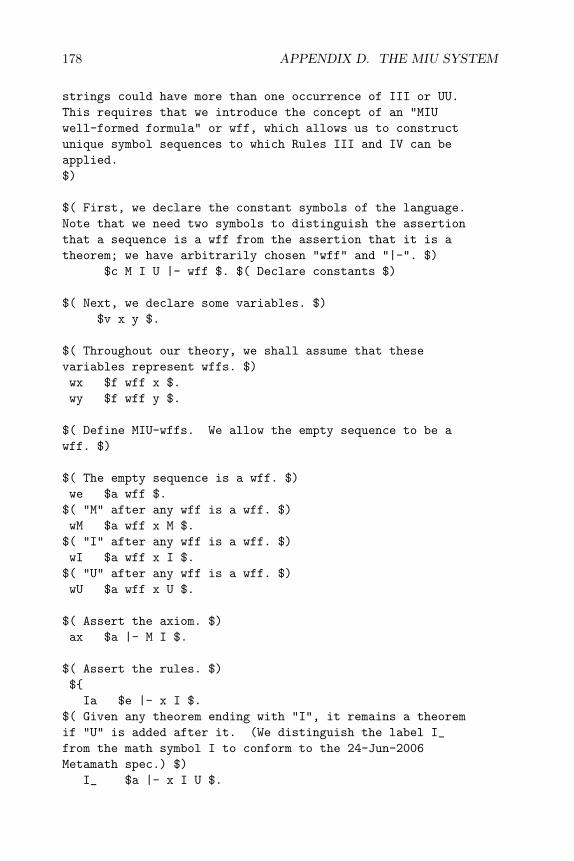
178 APPENDIX D. THE MIU SYSTEM
strings could have more than one occurrence of III or UU.
This requires that we introduce the concept of an "MIU
well-formed formula" or wff, which allows us to construct
unique symbol sequences to which Rules III and IV can be
applied.
$)
$( First, we declare the constant symbols of the language.
Note that we need two symbols to distinguish the assertion
that a sequence is a wff from the assertion that it is a
theorem; we have arbitrarily chosen "wff" and "|-". $)
$c M I U |- wff $. $( Declare constants $)
$( Next, we declare some variables. $)
$v x y $.
$( Throughout our theory, we shall assume that these
variables represent wffs. $)
wx $f wff x $.
wy $f wff y $.
$( Define MIU-wffs. We allow the empty sequence to be a
wff. $)
$( The empty sequence is a wff. $)
we $a wff $.
$( "M" after any wff is a wff. $)
wM $a wff x M $.
$( "I" after any wff is a wff. $)
wI $a wff x I $.
$( "U" after any wff is a wff. $)
wU $a wff x U $.
$( Assert the axiom. $)
ax $a |- M I $.
$( Assert the rules. $)
${
Ia $e |- x I $.
$( Given any theorem ending with "I", it remains a theorem
if "U" is added after it. (We distinguish the label I_
from the math symbol I to conform to the 24-Jun-2006
Metamath spec.) $)
I_ $a |- x I U $.

179
$}
${
IIa $e |- M x $.
$( Given any theorem starting with "M", it remains a theorem
if the part after the "M" is added again after it. $)
II $a |- M x x $.
$}
${
IIIa $e |- x I I I y $.
$( Given any theorem with "III" in the middle, it remains a
theorem if the "III" is replaced with "U". $)
III $a |- x U y $.
$}
${
IVa $e |- x U U y $.
$( Given any theorem with "UU" in the middle, it remains a
theorem if the "UU" is deleted. $)
IV $a |- x y $.
$}
$( Now we prove the theorem MUIIU. You may be interested in
comparing this proof with that of Hofstadter (pp. 35 - 36).
$)
theorem1 $p |- M U I I U $=
we wM wU wI we wI wU we wU wI wU we wM we wI wU we wM
wI wI wI we wI wI we wI ax II II I_ III II IV $.
The show proof /essential/lemmon/renumber command yields thefollowing display. It is very similar to the one in [24, pp. 35–36].
1 ax $a |- M I
2 1 II $a |- M I I
3 2 II $a |- M I I I I
4 3 I_ $a |- M I I I I U
5 4 III $a |- M U I U
6 5 II $a |- M U I U U I U
7 6 IV $a |- M U I I U
We note that Hofstadter’s “MU-puzzle,” which asks whether MU is atheorem of the MIU-system, cannot be answered using the system abovebecause the MU-puzzle is a question about the system. To prove the answerto the MU-puzzle, a much more elaborate system is needed, namely one thatmodels the MIU-system within set theory. (Incidentally, the answer to theMU-puzzle is no.)
180 APPENDIX D. THE MIU SYSTEM

Bibliography
[1] Donald J. Albers and G. L. Alexanderson, editors. Mathematical People.Contemporary Books, Inc., Chicago, 1985. [QA28.M37].
[2] Alan Ross Anderson and Nuel D. Belnap. Entailment, volume 1. Prince-ton University Press, Princeton, 1975. [QA9.A634 1975 v.1].
[3] John D. Barrow. Theories of Everything: The Quest for Ultimate Ex-planation. Oxford University Press, Oxford, 1991. [Q175.B225].
[4] H. Behnke, F. Backmann, K. Fladt, and W. Suss, editors. Fundamentalsof Mathematics, volume I. The MIT Press, Cambridge, Massachusetts,1974. [QA37.2.B413].
[5] J. L. Bell and M. Machover. A Course in Mathematical Logic. North-Holland, Amsterdam, 1977. [QA9.B3953].
[6] Andrea Blass. The interaction between category theory and set theory.In John Walter Gray, editor, Mathematical Applications of CategoryTheory (Proceedings of the Special Session on Mathematical Applica-tions Category Theory, 89th Annual Meeting of the American Mathe-matical Society, held in Denver, Colorado January 5–9, 1983), pages5–29, Providence, Rhode Island, 1983. American Mathematical Society.[QA169.A47 1983].
[7] W. W. Bledsoe and D. W. Loveland, editors. Automated Theorem Prov-ing: After 25 Years (Proceedings of the Special Session on AutomaticTheorem Proving, 89th Annual Meeting of the American Mathemati-cal Society, held in Denver, Colorado January 5–9, 1983), Providence,Rhode Island, 1983. American Mathematical Society. [QA76.9.A96.S641983].
[8] George S. Boolos and Richard C. Jeffrey. Computability and Log-ic. Cambridge University Press, Cambridge, third edition, 1989.[QA9.59.B66 1989].
[9] John Campbell. Programmer’s Progress. White Star Software, Box51623, Palo Alto, CA 94303, 1991.
181

182 BIBLIOGRAPHY
[10] Shang-Ching Chou. Proving elementary geometry theorems using Wu’salgorithm. In W. W. Bledsoe and D. W. Loveland, editors, AutomatedTheorem Proving: After 25 Years (Proceedings of the Special Sessionon Automatic Theorem Proving, 89th Annual Meeting of the AmericanMathematical Society, held in Denver, Colorado January 5–9, 1983),pages 243–286, Providence, Rhode Island, 1983. American Mathemati-cal Society. [QA76.9.A96.S64 1983].
[11] Richard Courant and Herbert Robbins. Topology. In James R. New-man, editor, The World of Mathematics, Volume One, pages 573–590.Simon and Schuster, New York, 1956. [QA3.W67 1988].
[12] Haskell B. Curry. Foundations of Mathematical Logic. Dover Publica-tions, Inc., New York, 1977. [QA9.C976 1977].
[13] Philip J. Davis and Reuben Hersh. The Mathematical Experience.Birkhauser Boston, Boston, 1981. [QA8.4.D37 1982].
[14] Richard de Millo, Richard Lipton, and Alan Perlis. Social processes andproofs of theorems and programs. In Thomas Tymoczko, editor, NewDirections in the Philosophy of Mathematics, pages 267–285. BirkhauserBoston, Inc., Boston, 1986. [QA8.6.N48 1986].
[15] Robert E. Edwards. A Formal Background to Mathematics. Springer-Verlag, New York, 1979. [QA37.2.E38 v.1a].
[16] Herbert B. Enderton. Elements of Set Theory. Academic Press, Inc.,San Diego, 1977. [QA248.E5].
[17] R. L. Goodstein. Development of Mathematical Logic. Springer-VerlagNew York Inc., New York, 1971. [QA9.G6554].
[18] Michael Guillen. Bridges to Infinity. Jeremy P. Tarcher, Inc., LosAngeles, 1983. [QA93.G8].
[19] Alan G. Hamilton. Logic for Mathematicians. Cambridge UniversityPress, Cambridge, revised edition, 1988. [QA9.H298].
[20] John Robert Harrison. Metatheory and reflection in theorem proving:A survey and critique. Technical Report CRC-053. SRI Cambridge,Millers Yard, Cambridge, UK, 1995. Available on the Web as http:-//www.cl.cam.ac.uk/users/jrh/papers/reflect.html.
[21] John Robert Harrison. Theorem proving with the real numbers. Tech-nical Report 408, University of Cambridge Computer Laboratory, NewMuseums Site, Pembroke Street, Cambridge, CB2 3QG, UK, 1996. Au-thor’s PhD thesis, available on the Web at http://www.cl.cam.ac.uk-/users/jrh/papers/thesis.html.
BIBLIOGRAPHY 183
[22] Horst Herrlich and George E. Strecker. Category Theory: An Introduc-tion. Allyn and Bacon Inc., Boston, 1973. [QA169.H567].
[23] J. Roger Hindley and David Meredith. Principal type-schemes andcondensed detachment. The Journal of Symbolic Logic, 55:90–105, 1990.[QA.J87].
[24] Douglas R. Hofstadter. Godel, Escher, Bach. Basic Books, Inc., NewYork, 1979. [QA9.H63 1980].
[25] D. Kalish and R. Montague. On Tarski’s formalization of predicatelogic with identity. Archiv fur Mathematische Logik und Grundlagenfor-schung, 7:81–101, 1965. [QA.A673].
[26] J. A. Kalman. Condensed detachment as a rule of inference. StudiaLogica, 42(4):443–451, 1983. [B18.P6.S933].
[27] Morris Kline. Mathematical Thought from Ancient to Modern Times.Oxford University Press, New York, 1972. [QA21.K516 1990 v.3].
[28] Morris Kline. Mathematics, The Loss of Certainty. Oxford UniversityPress, New York, 1980. [QA21.K525].
[29] Edna E. Kramer. The Nature and Growth of Modern Mathematics.Princeton University Press, Princeton, New Jersey, 1981. [QA93.K891981].
[30] Edmund Landau. Foundations of Analysis. Chelsea Publishing Com-pany, New York, second edition, 1960. [QA241.L2541 1960].
[31] Hugues Leblanc. On Meyer and Lambert’s quantificational calculusFQ. The Journal of Symbolic Logic, 33:275–280, 1968. [QA.J87].
[32] Czeslaw Lejewski. On implicational definitions. Studia Logica, 8:189–208, 1958. [B18.P6.S933].
[33] Adrian R. D. Mathias. A term of length 4,523,659,424,929. Synthese,133:75–86, 2002. [Q.S993].
[34] Norman D. Megill. A finitely axiomatized formalization of predicatecalculus with equality. Notre Dame Journal of Formal Logic, 36:435–453, 1995. [QA.N914].
[35] Norman D. Megill and Martin W. Bunder. Weaker D-complete logics.Journal of the IGPL, 4:215–225, 1996. Available on the Web at http:-//www.mpi-sb.mpg.de/igpl/Journal/V4-2/#Megill.
[36] Elliott Mendelson. Introduction to Mathematical Logic. D. Van Nos-trand Company, Inc., New York, second edition, 1979. [QA9.M5371979].

184 BIBLIOGRAPHY
[37] C. A. Meredith. Single axioms for the systems (C,N), (C,O) and (A,N)of the two-valued propositional calculus. The Journal of ComputingSystems, 3:155–164, 1953.
[38] David Meredith. In memoriam Carew Arthur Meredith (1904-1976).Notre Dame Journal of Formal Logic, 18:513–516, 1977. [QA.N914].
[39] J. Donald Monk. Substitutionless predicate logic with identity. Archivfur Mathematische Logik und Grundlagenforschung, 7:103–121, 1965.
[40] A. W. Moore. The Infinite. Routledge, New York, 1989. [BD411.M59].
[41] James R. Munkres. Topology: A First Course. Prentice-Hall, Inc.,Englewood Cliffs, New Jersey, 1975. [QA611.M82].
[42] E. Z. Nemesszeghy and E. A. Nemesszeghy. On strongly creative defini-tions: A reply to V. F. Rickey. Logique et Analyse (N. S.), 20:111–115,1977. [BC.L832].
[43] I. Nemeti. Algebraizations of quantifier logics, an overview. Ver-sion 11.4, preprint, Mathematical Institute, Budapest, 1994. A short-ened version without proofs appeared in “Algebraizations of quanti-fier logics, an introductory overview,” Studia Logica, 50:485–569, 1991[B18.P6.S933].
[44] M. Pavicic. A new axiomatization of unified quantum logic. Interna-tional Journal of Theoretical Physics, 31:1753 –1766, 1992. [QC.I626].
[45] Roger Penrose. The Emperor’s New Mind. Oxford University Press,New York, 1989. [Q335.P415].
[46] Ivars Peterson. The Mathematical Tourist. W. H. Freeman and Com-pany, New York, 1988. [QA93.P475].
[47] Jeremy George Peterson. An automatic theorem prover for substitutionand detachment systems. Notre Dame Journal of Formal Logic, 19:119–122, 1978. [QA.N914].
[48] Willard Van Orman Quine. Set Theory and Its Logic. The BelknapPress of Harvard University Press, Cambridge, Massachusetts, revisededition, 1969. [QA248.Q7 1969].
[49] J. A. Robinson. A machine-oriented logic based on the resolution prin-ciple. Journal of the Association for Computing Machinery, 12:23–41,1965.
[50] T. Thacher Robinson. Independence of two nice sets of axioms forthe propositional calculus. The Journal of Symbolic Logic, 33:265–270,1968. [QA.J87].

BIBLIOGRAPHY 185
[51] Rudy Rucker. Infinity and the Mind: The Science and Philosophy ofthe Infinite. Bantam Books, Inc., New York, 1982. [QA9.R79 1982].
[52] Bertrand Russell. Recent work on the principles of mathematics. In-ternational Monthly, 4:84, 1901.
[53] Bertrand Russell. Mysticism and Logic, and Other Essays. Barnes &Noble Books, Totowa, New Jersey, 1981. [B1649.R963.M9 1981].
[54] Joseph R. Shoenfield. Mathematical Logic. Addison-Wesley PublishingCompany, Inc., Reading, Massachusetts, 1967. [QA9.S52].
[55] Daniel Solow. How to Read and Do Proofs: An Introduction to Math-ematical Thought Process. John Wiley & Sons, New York, 1982.[QA9.S577].
[56] Harold M. Stark. An Introduction to Number Theory. Markham Pub-lishing Company, Chicago, 1970. [QA241.S72 1978].
[57] E. R. Swart. The philosophical implications of the four-color prob-lem. American Mathematical Monthly, 87:697–707, November 1980.[QA.A5125].
[58] George G. Szpiro. Poincare’s Prize: The Hundred-Year Quest to SolveOne of Math’s Greatest Puzzles. Penguin Books Ltd, London, 2007.[QA43.S985 2007].
[59] Gaisi Takeuti and Wilson M. Zaring. Introduction to Axiomatic SetTheory. Springer-Verlag New York Inc., New York, second edition,1982. [QA248.T136 1982].
[60] Alfred Tarski. What is elementary geometry. In Leon Henkin, PatrickSuppes, and Alfred Tarski, editors, The Axiomatic Method, with SpecialReference to Geometry and Physics (Proceedings of an InternationalSymposium held at the University of California, Berkeley, December26, 1957 — January 4, 1958), pages 16–29, Amsterdam, 1959. North-Holland Publishing Company.
[61] Alfred Tarski. A simplified formalization of predicate logic with iden-tity. Archiv fur Mathematische Logik und Grundlagenforschung, 7:61–79, 1965. [QA.A673].
[62] Thomas Tymoczko, editor. New Directions in the Philosophy of Math-ematics. Birkhauser Boston, Inc., Boston, 1986. [QA8.6.N48 1986].
[63] Hao Wang. Theory and practice in mathematics. In Thomas Tymoczko,editor, New Directions in the Philosophy of Mathematics, pages 129–152. Birkhauser Boston, Inc., Boston, 1986. [QA8.6.N48 1986].

186 BIBLIOGRAPHY
[64] Alfred North Whitehead. An Introduction to Mathematics, 1911.
[65] Alfred North Whitehead and Bertrand Russell. Principia Mathematica.Cambridge University Press, Cambridge, second edition, 1927. (3 vols.)[QA9.W592 1927].
[66] Stephen Wolfram. Mathematica: A System for Doing Mathematics byComputer. Addison-Wesley Publishing Co., Redwood City, California,second edition, 1991. [QA76.95.W65 1991].
[67] Larry Wos, Ross Overbeek, Ewing Lusk, and Jim Boyle. AutomatedReasoning: Introduction and Applications. McGraw-Hill, Inc., NewYork, second edition, 1992. [QA76.9.A96.A93 1992].
Index
$( and $) auxiliary keywords, 38,93, 97, 119
$. keyword, 38, 39, 46, 96, 98$= keyword, 39, 46, 96, 98, 107, 114,
124$[ and $] auxiliary keywords, 93,
97, 122, 135${ and $} keywords, 39, 96, 111, 112$a statement, 38, 39, 89, 94, 96, 98,
104, 106–108, 113–115,125, 135
$c statement, 38, 39, 93, 96, 99,100, 113
$d statement, 63, 65, 95, 96,100–102, 104, 105, 113,118, 141, 146
compound, 94simple, 94
$e statement, 38, 39, 94, 96, 98,105, 106, 113, 114, 135,138, 143, 146
$f statement, 38, 39, 45, 83, 94, 96,98, 105, 106, 113–115, 135,137, 145, 146
$p statement, 38, 39, 94, 96, 98,106, 107, 113–115, 117,124, 135, 136, 138
$t comment, 98, 119–121, 148, 155$v statement, 38, 39, 93, 96, 99,
100, 113[. . . ] inside comments, 121, 149_ inside comments, 121~ inside comments, 119, 121? in command lines, 46? inside proofs, 46, 124
‘ inside comments, 119, 121althtmldef statement, 149, 156althtmldir statement, 149assign command, 48, 143beep command, 133close log command, 132close tex command, 147delete command, 145erase command, 132exit command, 45, 131exthtmlbibliography statement,
150exthtmlhome statement, 150exthtmllabel statement, 150exthtmltitle statement, 150help command, 45htmlbibliography statement, 149htmldef statement, 148, 156htmldir statement, 149htmlhome statement, 149htmltitle statement, 149htmlvarcolors statement, 149improve command, 145initialize command, 145latexdef statement, 155let command, 143match command, 143minimize_with command, 53, 141more command, 133open log command, 131open tex command, 98, 147prove command, 47, 141read command, 41, 45, 46, 83, 134save new_proof command, 52, 124,
146
187

188 INDEX
save proof command, 90, 124, 138search command, 84, 88, 136set echo command, 132set empty_substitution
command, 49, 142set height command, 133set scroll command, 132set search_limit command, 142set unification_timeout
command, 141set width command, 132show trace_back command, 138show labels command, 42, 135show memory command, 135show new_proof command, 47, 142show proof command, 37, 42, 45,
46, 52, 86, 117, 118, 136show settings command, 135show statement command, 39, 42,
53, 63, 68, 84, 85, 135show trace_back command, 17, 88show usage command, 89, 137submit command, 45, 132tools command, 135, 151unify command, 144verify proof command, 41, 114,
124, 138write bibliography command,
151write recent_additions
command, 151write source command, 46, 134write theorem_list command,
150
abstract algebra, 3abstraction class, 56, 70, 174
of nested ordered pairs, 127of ordered pairs, 73
active math symbol, 93, 100, 113active statement, 94, 113addition, 127
of ordinals, 127ambiguous unification, 49, 119, 142,
146
analysis, 3, 29Anderson, Alan Ross, 17Andreka, H., 105, 164Appel, K., 23ascii, 33, 92, 96assertion, 39, 40, 94, 106, 114
in a formal system, 164assertion label, 40, 115, 118Auden, W. H., 5Aussonderung, 78automated proof verification, 19, 20automated theorem proving, 21, 26,
27, 61auxiliary keyword, 92, 96axiom, vii, 2, 17, 19, 29, 31, 34–38,
55, 57, 88, 89, 98, 107, 108,125, 126
Axiom of Choice, 17, 62, 66, 174Axiom of Extensionality, 62, 65, 67,
71, 174Axiom of Infinity, 32, 62, 66, 80, 174Axiom of Pairing, 62, 78Axiom of Power Sets, 62, 65, 174Axiom of Regularity, 62, 66, 174Axiom of Replacement, 62, 65, 174Axiom of Separation, 62, 78Axiom of the Null Set, 32, 62, 78Axiom of Union, 62, 65, 174axiom scheme, 35, 59, 63axiom vs. definition, 89, 107, 125,
126axiomatic assertion, 39, 106axiomatic statement
in a formal system, 165axioms for mathematics, 58axioms in set.mm, 64axioms of equality, 61, 64axioms of logic, 56axioms of predicate calculus, 60, 64axioms of propositional calculus, 58,
64axioms of set theory, 62, 65
Barrow, John D., xibasic keyword, 96

INDEX 189
basic language, 96, 99, 114, 138, 146Behnke, H., 30, 125Bell, J. L., 68Bible, 16biconditional (↔), 65, 67, 68, 173binary relation, 73, 81Blass, Andrea, 31Bledsoe, W. W., 27block, 39, 93, 112
outermost, 93Boolean algebra, 26Boolos, George S., 15, 17bound variable, 32, 100Bourbaki, Nicolas, xi, 15brace notation, 56Bunder, Martin, 17Burali-Forti paradox, 79
Cantor’s theorem, 79Cantor, Georg, 23cardinal, inaccessible, xii, 31cardinal, transfinite, 23cardinality, 23category theory, xii, 29, 31certainty, 18Chou, Shang-Ching, 25class, 67, 70
proper, 70, 174class abstraction, 56, 70, 174class difference, 72class equality, 71class membership, 71class variable, 174Clifford algebras, 24closure, 165Cohen, Paul, 23collection, 61command keyword, 41, 45, 83command line interface (CLI), 40,
45command qualifier, 42comment, 93, 119comments
markup notation, 119, 121compact proof, 89
composition, 75compound declaration, 100compressed proof, 40, 52, 95, 123,
124, 159computer algebra system, 3, 21, 24computer program bugs, viii, 8, 12,
19, 21, 22, 25computers and pure mathematics,
21concatenation, 162condensed detachment, 31
and first-order logic, 31conjunction (∧), 65, 69, 87, 173connective, 68consistent theory, 18constant, x, 38, 40, 68, 93, 99, 113
in a formal system, 162in predicate calculus, 64
constant declaration, 38, 39, 99constant-prefixed expression, 163constant-variable pair, 163constructive language, 20constructivism, 17continuum hypothesis, 23Courant, Richard, 23Courier font, 33Coxeter, H. S. M., 24cranks, 13creative definition, 67, 125cross product, 74Curry, Haskell B., 18
database, 38, 92, 96, 134Davis, Phillip J., 1, 12, 14, 30de Millo, Richard, 15de Saint-Exupery, Antoine, 161decidable theory, 25decision procedure, 61declaration, 93deduction theorem, 11definiendum, 67definiens, 67definition, 15, 66, 88, 89, 98, 107,
125, 126, 172creative, 67, 125
190 INDEX
eliminability, 67proper, 108, 125
disjoint sets, 62disjoint variables, 63, 101disjoint-variable restriction, 94
in a formal system, 164disjunction (∨), 69, 125, 173distinct variables, 32, 63, 65, 100,
103domain, 23, 74dummy variable, 85, 110
eliminating, 27, 105in definitions, 67
Edwards, Robert E., 14effectively bound variable, 67effectively not free, 76, 170element, 61empty domain, 32empty set, 56, 72, 175empty substitution, 101, 142Enderton, Herbert B., 17, 23, 68, 84epsilon relation, 73equality (=), 60, 61, 67error checking, 122, 148errors in proofs, 22, 24essential hypothesis, 39, 105Euclidean geometry, xi, 23, 25existential quantifier (∃), 65, 69, 173
restricted, 71existential uniqueness quantifier
(∃!), 70expression, 95, 99
in a formal system, 163extended frame, 110extended language, 97, 119
family, 61Feferman, Solomon, xiiFermat’s Last Theorem, 13, 23, 25file inclusion, 93, 122file names
Macintosh, 41, 123Unix, 41, 129, 134
finitary proof, 29, 30
finite n-termed sequence, 162finite induction, 79first-order logic, 11, 20, 26, 31, 56
completeness, 11floating hypothesis, 39, 105formal logic, 19, 107formal proof, x, 12, 13, 15, 19, 20,
32, 34, 36, 37, 42, 44, 46,48
formal system, vii, ix, 2, 19, 29, 142,165, 177
formalism, 30foundations of mathematics, 17founded relation, 73four-color theorem, 21, 23frame, 108frames and scoping statements, 114free logic, 32free variable, 32, 60, 61, 63, 100,
106, 170free vs. bound variable, 100Frege, Gottlob, 18function, 23, 75
in predicate calculus, 64function value, 76
Godel’s incompleteness theorem, ix,5, 15, 18
gaps in proofs, 19Ghilbert, xiiglobal statement, 113Goodstein, R. L., 126grave accent (‘), 119, 120Grothendieck, Alexander, xiigroup theory, 3Guillen, Michael, 5
Haken, W., 23Halmos, Paul, 21Hamilton, Alan G., 60, 86Hardy, G. H., 92Harrison, John, 20, 25Herrlich, Horst, 31hierarchy, 13, 15, 19, 26, 88higher-order logic, 20, 29
INDEX 191
Hilbert, David, 15, 16, 23, 29, 30Hindley, J. Roger, 31Hofstadter, Douglas R., 29, 36, 179hol, 27, 28html generation, 121, 136, 156Hume, David, 22Huntington, E. V., 26hypothesis, 39, 94, 105hypothesis association, 118hypothesis label, 40, 115
iff, 73image, 75implication (→), 34, 58implicit axiom, 32included file, 93, 122individual metavariable, 168individual variable, 59inference, 106, 167inference rule, 35infinite set, 56infinity, 23infix connective, 70informal proof, 13, 15integer, 56, 57intersection, 72, 73intuitionism, 17, 29, 126Isabelle, 27
Kalman, J. A., 31Kempe, A. B., 23keyword, 38, 92, 96, 97Kline, Morris, 18, 30Koch, K., 23Kronecker, Leopold, 16Kuratowski, Kazimierz, 73
label, 39, 42, 45, 93, 96, 98, 103,105, 107, 108, 115, 118
label declaration, 98label mode, 120, 121label reference, 98, 114label sequence, 98, 114labels in set.mm, 89Landau, Edmund, 5
LATEX, ix, 34, 85, 98, 119, 137, 147,148
characters per line, 133LATEX definitions, 155lcf, 28Lesniewski, S., 125Leblanc, Hugues, 32Lejewski, Czeslaw, 125Lemmon-style proof, 43length of a sequence (| |), 162Levien, Raph, xiilimit ordinal, 74local label, 90local variable, 113logic, 2logical equivalence (↔), 65, 67, 68,
173logical hypothesis, 39, 105
in a formal system, 164logical and (∧), 65, 69, 87logical or (∨), 69Lounesto, Pertti, 24
Mac Lane, Saunders, xiiMacintosh file names, 41, 123macsyma, 3mandatory $d statement, 118mandatory disjoint-variable
restriction, 94in a formal system, 164
mandatory hypothesis, 39, 42, 53,94, 110, 115, 117, 118, 124
in a formal system, 164mandatory variable, 94, 109mandatory variable-type hypothesis
in a formal system, 164Maple, 3, 25mapping, 23markup notation, 119, 121math mode, 119, 120math symbol, 38, 39, 44, 45, 60, 93,
96–99, 113, 120Mathematica, 3, 24Mathematica and proofs, 25mathematical induction, 79
192 INDEX
Mathias, Adrian R. D., 15Megill, Norman, 17, 27, 31, 32, 64,
105, 171member, 61Mendelson, Elliot, 34, 36Meredith, C. A., 31, 58metalanguage, 2, 17, 29metalogic, 64, 126metalogical completeness, 32, 170,
171Metamath, vii–xi, 2–4, 15–17, 19,
20, 22, 24, 26, 29–31, 34,35, 37, 38, 40, 41, 45, 46,55, 58–61, 63, 83, 91,96–99, 103, 106, 107, 118,120–123, 125
as a formal system, 161bugs, 131commands, 129installation, 33limitations of version 0.07.30,
89, 92, 119, 134, 141, 148,150, 155
memory limits, 134memory usage, 135representation of numbers, 3self-description, 20specification, 92using as a math editor, 120
metamathematics, 30metatheorem, 12, 32metavariable, 34, 37–39, 60, 99, 101Millay, Edna, 16MIU-system, 29, 49, 142, 177Miyaoka, Yoichi, 23Mizar, xiii, 28modal logic, 17, 29model theory, 29modus ponens, 35, 36, 59, 64Monaco font, 33Monk, J. Donald, 32monospaced font, 33Munkres, James R., 3, 161
natural number, 56, 66, 74, 80, 127
negation (¬), 58Nemesszeghy, E. Z., 125nested block, 112nesting level, 112non-scoping statement, 112non-trivial theory, 100normal proof, 40, 52, 123null set, 72number theory, 2, 34
object, 61object language, 17omega (ω), 57, 66, 74, 80one-to-one function, 75onto function, 75operating system command, 133operation, 76, 81operator precedence, 35optional disjoint-variable restriction,
110optional hypothesis, 85, 110optional variable, 85, 110ordered pair, 73ordinal addition, 127ordinal number, 74ordinal predicate, 74otter, 27outermost block, 112, 113, 123
pair, 72parsing Metamath, 92Pasch’s axiom, xi, 23Pavicic, M., 17Peano’s postulates, 66, 79Penrose, Roger, 26Perelman, Grigory, 24Peterson, Jeremy George, 31Pierce’s axiom, 120plain text, 33Poincare conjecture, 24Polish notation, 70pop, 40, 115postfix connective, 70power class, 72power set, 72
INDEX 193
pre-statementin a formal system, 164
predicate calculus, 56, 59, 168prefix connective, 70Principia Mathematica, 30printable character, 96printers, 33proof, 25, 35, 98, 114
compressed, 40, 52, 95, 123,124, 159
Lemmon-style, 43Metamath, 95Metamath, description of, 114normal, 40, 52, 123tree-style, 43, 117
Proof Assistant, ix, 46–48, 51, 52,119, 124, 131, 139, 141,142, 144–146
proof length, 15, 21, 89proof scheme, 35proof step, 37proof theory, 29proper class, 70, 174proper definition, 108, 125proper substitution, 32, 60, 63, 69,
100, 170propositional calculus, 31, 56, 58,
166provable assertion, 39, 106provable statement
in a formal system, 165Purinton, Josh, xii, 165push, 40, 115
qed project, 28qualifying expression, 67quantifier theory, 56quantum logic, 3, 17, 29quantum mechanics, 3Quine, Willard Van Orman, 17, 68,
126, 174
Rego, Eduardo, 24range, 75rational number, 57
real and complex numbers, 3, 29axioms for, 80
real number, 57recursion operator, 127recursive definition, 112, 126, 127redeclaration of symbols, 39, 94, 113reduct
in a formal system, 164reflection principle, 20relation, 75restriction, 75reverse Polish notation (RPN), 35,
115Robbins algebra, 26Robbins, Herbert, 26Robinson’s resolution principle, 26,
31Robinson, T. Thacher, 126Rourke, Colin, 24RPN order, 42, 110, 160RPN stack, 40, 95, 115, 118Rucker, Rudy, 6, 36, 55rule, vii, 17, 31, 36, 59, 108rule of generalization, 61, 64Russell’s paradox, 9, 10, 18, 79Russell, Bertrand, 15, 30, 91
Schroder-Bernstein theorem, 23scope, 85, 100, 113scoping statement, 93, 112sentential logic, 56set, 23, 61set difference, 72set intersection, 56set theory, 2, 19, 29, 56, 61set theory database (set.mm), 16,
27, 29, 31–33, 58–61, 63,76, 83, 126, 148, 150, 155,174, 176
set union, 56Shoenfield, Joseph R., 30simple declaration, 99simple infinite sequence, 162simple metatheorem, 171singleton, 72

194 INDEX
Solovay, Robert, xiiSolow, Daniel, 8source buffer, 46, 138, 146source file, 96, 97, 122, 134special characters, 92stack, 40, 95, 115, 118Stark, Harold M, 23statement
in a formal system, 164stylized epsilon (∈), 57, 60subclass, 72subset, 62, 72substitution
implicit, 77proper, 32, 60, 63, 69, 100, 170variable, x, 31, 37, 39, 40, 47,
49, 63, 86, 87, 95, 99, 115,118, 142, 163
substitution map, 95, 163substitution theorem, 11successor, 74, 79, 126Swart, E. R., 21symbol, 96
in a formal system, 162syntax rules, 19, 34Szpiro, George, 24
Takeuti, Gaisi, 68, 174Tarski, Alfred, 25, 26, 32, 162tautology, 59temporary variable, 48, 141, 144term, 34, 37, 162text editor, 33theorem, vii, 19, 25, 29, 31, 34–36,
38, 47, 55, 57, 59, 61, 106,125
theorem scheme, 35tilde (~), 119, 121token, 38, 45, 46, 92, 96–99,
119–122, 134topology, 3transfinite recursion, 80transitive class, 73transitive set, 73tree-style proof, 43, 117
trusting computers, 21truth table, 59turnstile (`), 38, 76, 98, 106Tymoczko, Thomas, 17, 21type, 99, 105typesetting comment, 98, 119–121,
148, 155
Ulam, Stanislaw, 22unification, 31, 47, 118
ambiguous, 49, 119, 142, 146union, 72, 73, 175universal class (V ), 72universal quantifier (∀), 60
restricted, 71universe of a formal system, 165Unix file names, 41, 129, 134unordered pair, 72, 175unordered triple, 72
variable, x, 39, 40, 99, 101, 113in a formal system, 162in ordinary mathematics, 101in predicate calculus, 56, 59in set theory, 57, 61Metamath, 93
variable declaration, 38, 39, 99variable substitution, x, 31, 37, 39,
40, 47, 49, 63, 86, 87, 95,99, 115, 118, 142, 163
variable type, 99, 105variable-type hypothesis, 39, 105
in a formal system, 164Venn diagram, 62
Wang, Hao, 14weak logic, 17, 20, 29well-formed formula (wff), vii, 19,
20, 34, 37, 58, 60, 63, 83,116, 125, 179
well-ordering, 74Wen-tsun, Wu, 25white space, 92, 96, 119–121, 124Whitehead, Alfred North, 4, 30Wiles, Andrew, 23

INDEX 195
Williams, Anthony, xiiiWord (Microsoft), 33word processor, 33Wos, Larry, 26, 27
Zermelo-Fraenkel set theory, 9, 32,56, 61
ZFC set theory, 63, 173