—A B B M E A SU R EM ENT & A N A LY TI C S | W H ITE PA PER

The measurement of turbidity and suspended solids in wastewater

An introduction to the causes of turbidity in water, describing how turbidity is measured and how the measurement of turbidity can be used to infer the suspended solids content in water

Measurement made easy

—Why is water turbid

We say that a particular water sample is turbid when the sample is hazy or cloudy. The main effect of the haziness is that we cannot see clearly through the sample after a certain distance, as the distance over which it is possible to see clearly decreases as the turbidity increases.

Turbidity is caused by material suspended in the water, which can scatter or absorb light traveling through the water. Scattering is the process by which light traveling in one direction is deflected by particles in suspension into a different direction of travel. Absorption is the reduction in the intensity of light as it travels through the sample. In general the effect of turbidity is to increase the amount of light seen at an angle with respect to the propagation of the illumination, and a reduction in the amount of light seen through the sample, as shown in Figure 1.

Transmitted light

Scattered light

Absorbed light

Figure 1 Transmission, absorption and scattering of light by a turbid sample.

—A brief introduction to light scattering

2 TH E M E A S U R E M E NT O F TU R B I D IT Y A N D S U S PE N D E D S O LI DS I N WA S TE WATE R | W P/A N A I NS T/0 0 2- EN

—…Why is water turbid

In general, light is scattered by particles in suspension, such as sand, organic particles, or microorganisms, whereas absorption is due to dissolved materials. The presence of dissolved materials that absorb light is generally indicated by color in the sample.

The presence of absorbing material affects the light equally in all directions, and has the effect of reducing the light intensity measured in any given direction for the particular wavelengths at which the material absorbs, while other wavelengths are unaffected. This selective absorption leads to the brownish color of water that contains a significant amount of dissolved organic matter, because the dissolved organic matter absorbs the light in the blue end of the spectrum, leaving the red unaffected.

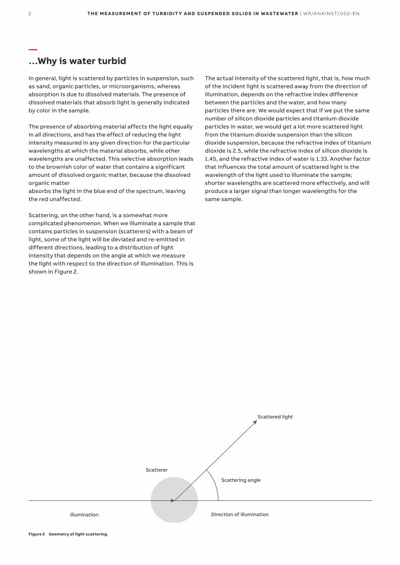
Scattering, on the other hand, is a somewhat more complicated phenomenon. When we illuminate a sample that contains particles in suspension (scatterers) with a beam of light, some of the light will be deviated and re-emitted in different directions, leading to a distribution of light intensity that depends on the angle at which we measure the light with respect to the direction of illumination. This is shown in Figure 2.

The actual intensity of the scattered light, that is, how much of the incident light is scattered away from the direction of illumination, depends on the refractive index difference between the particles and the water, and how many particles there are. We would expect that if we put the same number of silicon dioxide particles and titanium dioxide particles in water, we would get a lot more scattered light from the titanium dioxide suspension than the silicon dioxide suspension, because the refractive index of titanium dioxide is 2.5, while the refractive index of silicon dioxide is 1.45, and the refractive index of water is 1.33. Another factor that influences the total amount of scattered light is the wavelength of the light used to illuminate the sample; shorter wavelengths are scattered more effectively, and will produce a larger signal than longer wavelengths for the same sample.

Scattered light

Scattering angle

Scatterer

Illumination Direction of illumination

Figure 2 Geometry of light scattering.

3TH E M E A S U R E M E NT O F TU R B I D IT Y A N D S U S PE N D E D S O LI DS I N WA S TE WATE R | W P/A N A I NS T/0 0 2- EN

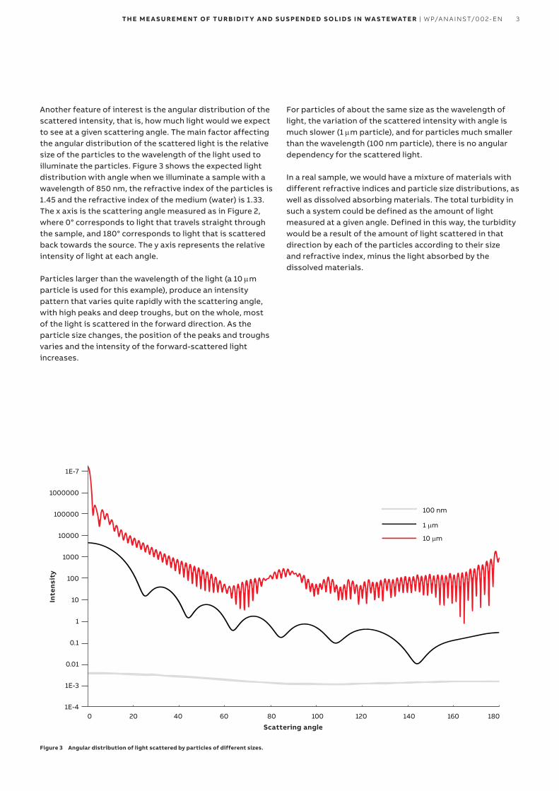
Another feature of interest is the angular distribution of the scattered intensity, that is, how much light would we expect to see at a given scattering angle. The main factor affecting the angular distribution of the scattered light is the relative size of the particles to the wavelength of the light used to illuminate the particles. Figure 3 shows the expected light distribution with angle when we illuminate a sample with a wavelength of 850 nm, the refractive index of the particles is 1.45 and the refractive index of the medium (water) is 1.33. The x axis is the scattering angle measured as in Figure 2, where 0° corresponds to light that travels straight through the sample, and 180° corresponds to light that is scattered back towards the source. The y axis represents the relative intensity of light at each angle.

Particles larger than the wavelength of the light (a 10 µm particle is used for this example), produce an intensity pattern that varies quite rapidly with the scattering angle, with high peaks and deep troughs, but on the whole, most of the light is scattered in the forward direction. As the particle size changes, the position of the peaks and troughs varies and the intensity of the forward-scattered light increases.

For particles of about the same size as the wavelength of light, the variation of the scattered intensity with angle is much slower (1 µm particle), and for particles much smaller than the wavelength (100 nm particle), there is no angular dependency for the scattered light.

In a real sample, we would have a mixture of materials with different refractive indices and particle size distributions, as well as dissolved absorbing materials. The total turbidity in such a system could be defined as the amount of light measured at a given angle. Defined in this way, the turbidity would be a result of the amount of light scattered in that direction by each of the particles according to their size and refractive index, minus the light absorbed by the dissolved materials.

100 nm

1 µm

10 µm

Scattering angle

Inte

nsit

y

1E-7

1000000

100000

10000

1000

100

10

1

0.1

0.01

1E-3

1E-40 20 40 60 80 100 120 140 160 180

Figure 3 Angular distribution of light scattered by particles of different sizes.

4 TH E M E A S U R E M E NT O F TU R B I D IT Y A N D S U S PE N D E D S O LI DS I N WA S TE WATE R | W P/A N A I NS T/0 0 2- EN

—Measuring turbidity in practice

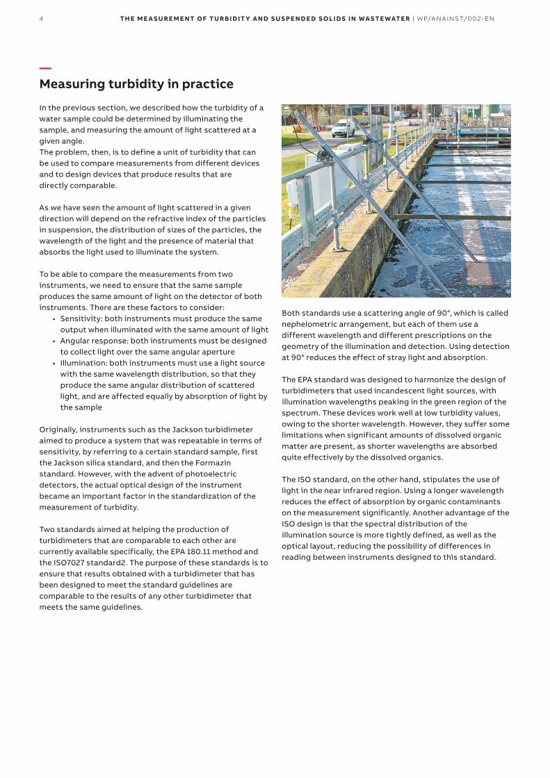
In the previous section, we described how the turbidity of a water sample could be determined by illuminating the sample, and measuring the amount of light scattered at a given angle. The problem, then, is to define a unit of turbidity that can be used to compare measurements from different devices and to design devices that produce results that are directly comparable.

As we have seen the amount of light scattered in a given direction will depend on the refractive index of the particles in suspension, the distribution of sizes of the particles, the wavelength of the light and the presence of material that absorbs the light used to illuminate the system.

To be able to compare the measurements from two instruments, we need to ensure that the same sample produces the same amount of light on the detector of both instruments. There are these factors to consider:

• Sensitivity: both instruments must produce the same output when illuminated with the same amount of light

• Angular response: both instruments must be designed to collect light over the same angular aperture

• Illumination: both instruments must use a light source with the same wavelength distribution, so that they produce the same angular distribution of scattered light, and are affected equally by absorption of light by the sample

Originally, instruments such as the Jackson turbidimeter aimed to produce a system that was repeatable in terms of sensitivity, by referring to a certain standard sample, first the Jackson silica standard, and then the Formazin standard. However, with the advent of photoelectric detectors, the actual optical design of the instrument became an important factor in the standardization of the measurement of turbidity.

Two standards aimed at helping the production of turbidimeters that are comparable to each other are currently available specifically, the EPA 180.11 method and the ISO7027 standard2. The purpose of these standards is to ensure that results obtained with a turbidimeter that has been designed to meet the standard guidelines are comparable to the results of any other turbidimeter that meets the same guidelines.

Both standards use a scattering angle of 90°, which is called nephelometric arrangement, but each of them use a different wavelength and different prescriptions on the geometry of the illumination and detection. Using detection at 90° reduces the effect of stray light and absorption.

The EPA standard was designed to harmonize the design of turbidimeters that used incandescent light sources, with illumination wavelengths peaking in the green region of the spectrum. These devices work well at low turbidity values, owing to the shorter wavelength. However, they suffer some limitations when significant amounts of dissolved organic matter are present, as shorter wavelengths are absorbed quite effectively by the dissolved organics.

The ISO standard, on the other hand, stipulates the use of light in the near infrared region. Using a longer wavelength reduces the effect of absorption by organic contaminants on the measurement significantly. Another advantage of the ISO design is that the spectral distribution of the illumination source is more tightly defined, as well as the optical layout, reducing the possibility of differences in reading between instruments designed to this standard.

5TH E M E A S U R E M E NT O F TU R B I D IT Y A N D S U S PE N D E D S O LI DS I N WA S TE WATE R | W P/A N A I NS T/0 0 2- EN

—Using turbidity to measure suspended solids

We have described how the turbidity of a sample is measured as the intensity of light scattered by the material suspended in the sample, and how the scattered light intensity is proportional to the number of suspended particles, the suspended solids. Based on this, we should be able to use the turbidity of a sample to infer the mass of particles in suspension that produce that level of turbidity. For a given sample, all that is needed is to produce a calibration curve that relates the mass of suspended solids to the turbidity. This relation will be linear, as shown in Figure 4.

In a general case, the slope of the linear relation will be sample dependent, as shown in Figure 4 and that slope would be very difficult to calculate theoretically, so it is normally determined by calibration.

Traditionally, the laboratory-based gravimetric procedure has been used for obtaining the data needed for calibration in accordance with ASTM method D5907-103. In this procedure, the solids are filtered out from the water before being dried and then weighed to produce a value in mg/l for total suspended solids. This measurement is then correlated with the turbidity measurement, with the resulting data being used to produce the calibration curve.

Turbidity (NTU)

Su

spen

ded

so

lids

con

ten

t (m

g/l

)

100,000

20,000

01000 2000 3000 4000 5000 60000

40,000

60,000

80,000

Kaolin

Fullers earth

SiO2

Figure 4 Relationship between suspended solids and turbidity for fullers earth and kaolin.

6 TH E M E A S U R E M E NT O F TU R B I D IT Y A N D S U S PE N D E D S O LI DS I N WA S TE WATE R | W P/A N A I NS T/0 0 2- EN

—The problem of achieving a reliable calibration

Whilst the gravimetric procedure can be useful when trying to establish a relationship between total suspended solids and turbidity, a single sample based on the technique will not, by itself, provide a complete or reliable picture of overall conditions. First and foremost, as a ‘one-off’ measurement, it will only ever be representative of a certain set of conditions at a certain moment in time. A measurement obtained using the technique will therefore only be effective as a general guide to an ideal set of conditions, which may not apply universally.

It is important to remember also that suspended solids levels can vary independently of the turbidity measurement. Turbidity, which is measured in NTU, provides a measurement of the impact of suspended solids on the passage of light through water. Total suspended solids, which is measured in mg/l, is a quantitative measurement of the concentration of suspended particles in a given sample. As such there is no single way of recognizing the differences in the size and/or composition of the suspended particles, or the impact that those particles may have on measuring turbidity.

A quantity of coal dust, for example, would have a different impact on turbidity than an identical quantity of silt, as they will scatter and absorb light in different ways.

For a given sample, it is possible to build a calibration curve to convert the turbidity value to a suspended solids value, as shown in Figure 4.

This has a particular impact on processes with changing conditions that could affect the composition of the sample.

Such changes will have a direct bearing on the calculation of the coefficients in the calibration curve. If the composition or the particle size distribution of the sample changes, the slope will also change and a new calibration will be required.

7TH E M E A S U R E M E NT O F TU R B I D IT Y A N D S U S PE N D E D S O LI DS I N WA S TE WATE R | W P/A N A I NS T/0 0 2- EN

—Calibration in practice

In a typical installation, the user will take grab samples from the process water, record the turbidity reading at the time, and measure the suspended solids content of the grab sample using a laboratory method such as ASTM D5907-10.

The turbidity reading taken at the time the grab sample was obtained and the suspended solids value from the laboratory method can then be used to calculate a conversion coefficient from turbidity to suspended solids as follows.

c = TSSTurb

In this equation, c is the conversion coefficient, TSS is the suspended solids content and Turb is the turbidity reading.

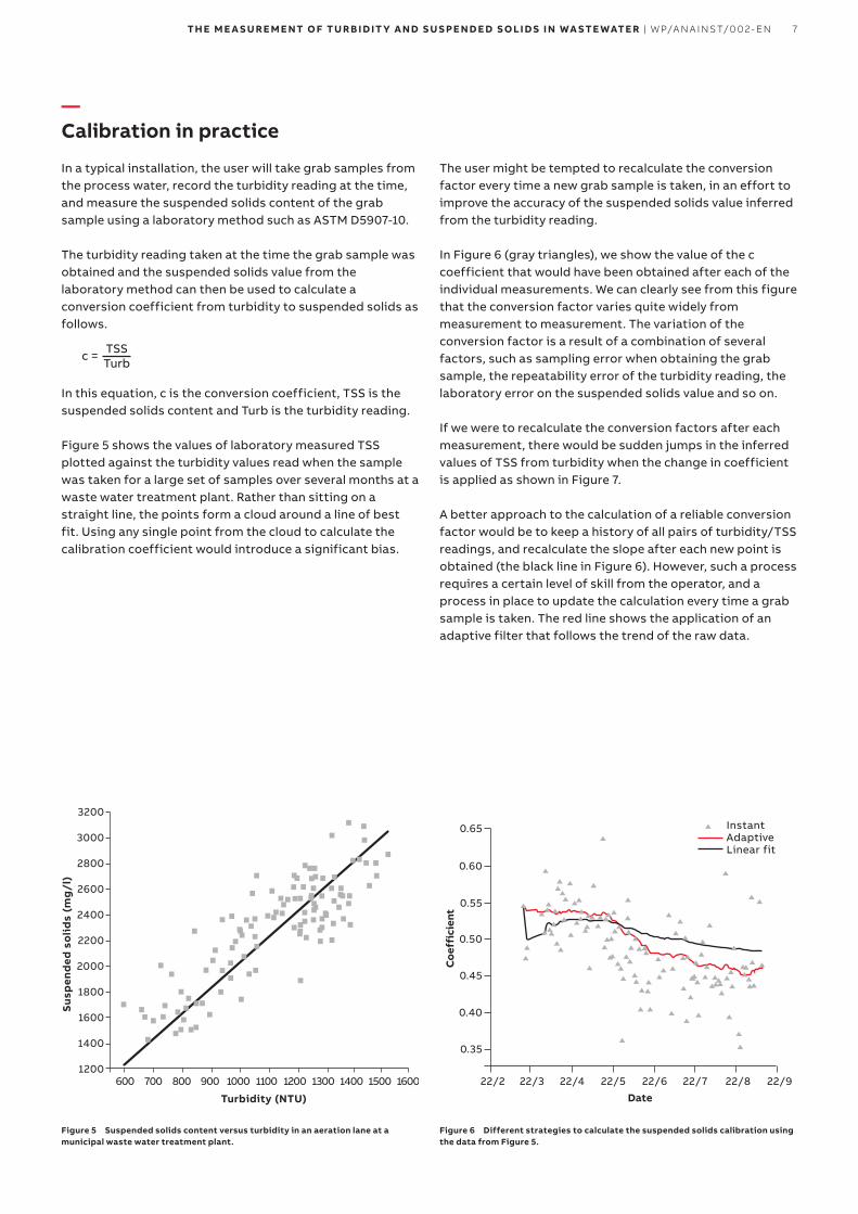
Figure 5 shows the values of laboratory measured TSS plotted against the turbidity values read when the sample was taken for a large set of samples over several months at a waste water treatment plant. Rather than sitting on a straight line, the points form a cloud around a line of best fit. Using any single point from the cloud to calculate the calibration coefficient would introduce a significant bias.

Turbidity (NTU)

Susp

end

ed s

olid

s (m

g/l

)

3200

3000

2600

2200

1800

1400

1600

1200600 700 800 900 1000 1100 1200 1300 1400 1500 1600

2000

2400

2800

Figure 5 Suspended solids content versus turbidity in an aeration lane at a municipal waste water treatment plant.

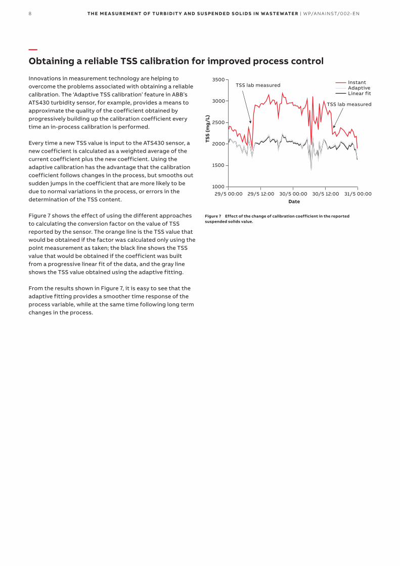
The user might be tempted to recalculate the conversion factor every time a new grab sample is taken, in an effort to improve the accuracy of the suspended solids value inferred from the turbidity reading.

In Figure 6 (gray triangles), we show the value of the c coefficient that would have been obtained after each of the individual measurements. We can clearly see from this figure that the conversion factor varies quite widely from measurement to measurement. The variation of the conversion factor is a result of a combination of several factors, such as sampling error when obtaining the grab sample, the repeatability error of the turbidity reading, the laboratory error on the suspended solids value and so on.

If we were to recalculate the conversion factors after each measurement, there would be sudden jumps in the inferred values of TSS from turbidity when the change in coefficient is applied as shown in Figure 7.

A better approach to the calculation of a reliable conversion factor would be to keep a history of all pairs of turbidity/TSS readings, and recalculate the slope after each new point is obtained (the black line in Figure 6). However, such a process requires a certain level of skill from the operator, and a process in place to update the calculation every time a grab sample is taken. The red line shows the application of an adaptive filter that follows the trend of the raw data.

0.65

0.60

0.55

0.50

0.45

0.40

0.35

InstantAdaptiveLinear fit

22/2 22/3 22/4 22/5 22/6 22/7 22/8 22/9

Date

Coe

ffic

ient

Figure 6 Different strategies to calculate the suspended solids calibration using the data from Figure 5.

8 TH E M E A S U R E M E NT O F TU R B I D IT Y A N D S U S PE N D E D S O LI DS I N WA S TE WATE R | W P/A N A I NS T/0 0 2- EN

—Obtaining a reliable TSS calibration for improved process control

Innovations in measurement technology are helping to overcome the problems associated with obtaining a reliable calibration. The ‘Adaptive TSS calibration’ feature in ABB’s ATS430 turbidity sensor, for example, provides a means to approximate the quality of the coefficient obtained by progressively building up the calibration coefficient every time an in-process calibration is performed.

Every time a new TSS value is input to the ATS430 sensor, a new coefficient is calculated as a weighted average of the current coefficient plus the new coefficient. Using the adaptive calibration has the advantage that the calibration coefficient follows changes in the process, but smooths out sudden jumps in the coefficient that are more likely to be due to normal variations in the process, or errors in the determination of the TSS content.

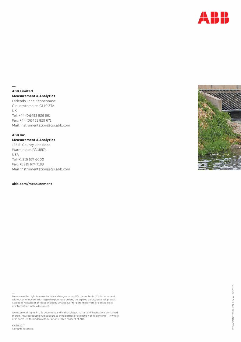
Figure 7 shows the effect of using the different approaches to calculating the conversion factor on the value of TSS reported by the sensor. The orange line is the TSS value that would be obtained if the factor was calculated only using the point measurement as taken; the black line shows the TSS value that would be obtained if the coefficient was built from a progressive linear fit of the data, and the gray line shows the TSS value obtained using the adaptive fitting.

From the results shown in Figure 7, it is easy to see that the adaptive fitting provides a smoother time response of the process variable, while at the same time following long term changes in the process.

3500TSS lab measured Instant

AdaptiveLinear fit

TSS lab measured3000

2500

2000

1500

100029/5 00:00 29/5 12:00 30/5 00:00 30/5 12:00 31/5 00:00

DateTS

S (m

g/L)

Figure 7 Effect of the change of calibration coefficient in the reported suspended solids value.

9TH E M E A S U R E M E NT O F TU R B I D IT Y A N D S U S PE N D E D S O LI DS I N WA S TE WATE R | W P/A N A I NS T/0 0 2- EN

—Introducing the ATS430 Turbidity and TSS sensor system

ABB’s ATS430 turbidity and TSS probe with adaptive TSS calibration provides operators with more reliable process data for improved process control and regulatory compliance.

Compact and robust, it uses the latest advances in optical measurement technology to deliver precise and ultra-stable measurement of turbidity and suspended solids concentrations up to 4000NTU (Nephelometric Turbidity Units) or 100,000 mg/l.

Its service-free design, plus features including in-situ cleaning, easy calibration and verification and predictive maintenance diagnostics, enables it to offer the lowest cost of ownership of any device on the market.

Available with a range of mounting options and in a choice of stainless steel or titanium for corrosive media, the ATS430 can be used in a wide range of utility and industrial applications, including:

• Potable water treatment• Municipal / industrial wastewater treatment• Produced and flowback wastewater treatment• Pulp & Paper• Marine• Mining

Key features at a glance:Easy to use• EZLink automatic sensor recognition and set-up for fast

and simple connection to ABB AWT440 digital transmitter• Advanced predictive maintenance diagnostics• Supplied factory-calibrated, ready for use

Accurate and reliable• Choice of stainless steel or titanium sensor bodies• Scratch-resistant sapphire windows• Adaptive TSS calibration for improved control• MCERTS approved

Lowest cost of ownership• No servicing for the lifetime of the sensor• In-situ cleaning• Easy calibration and verification

Flexible installation options• Pipe, tank, open channel or flow-cell options• Suitable for use in salt water and corrosive media

Compact design• 40 mm (1.57 in.) probe diameter, ideal for a range

of installations

ABB’s ATS430 incorporates a host of features offering accurate, reliable and stable measurement of turbidity and total suspended solids.

10 TH E M E A S U R E M E NT O F TU R B I D IT Y A N D S U S PE N D E D S O LI DS I N WA S TE WATE R | W P/A N A I NS T/0 0 2- EN

—References

1 Method for Determining the Turbidity of a Water Sample. US Environmental Protection Agency (EPA). Washington DC: EPA, 1979. 180.1.

2 Water Quality - Determination of Turbidity. ISO. Geneva: ISO, 1993. 7027.

3 Standard test methods for filterable matter (Total Dissolved Solids) and non-filterable matter (Total Suspended Solids) in water ASTM D5907-10.

11TH E M E A S U R E M E NT O F TU R B I D IT Y A N D S U S PE N D E D S O LI DS I N WA S TE WATE R | W P/A N A I NS T/0 0 2- EN

—Notes

WP/

AN

AIN

ST/

00

2-E

N R

ev. A

12

.20

17

—ABB Limited Measurement & Analytics Oldends Lane, Stonehouse Gloucestershire, GL10 3TA UK Tel: +44 (0)1453 826 661 Fax: +44 (0)1453 829 671 Mail: instrumentation@gb.abb.com

ABB Inc. Measurement & Analytics 125 E. County Line Road Warminster, PA 18974 USA Tel: +1 215 674 6000 Fax: +1 215 674 7183 Mail: instrumentation@gb.abb.com

abb.com/measurement

—We reserve the right to make technical changes or modify the contents of this document without prior notice. With regard to purchase orders, the agreed particulars shall prevail. ABB does not accept any responsibility whatsoever for potential errors or possible lack of information in this document.

We reserve all rights in this document and in the subject matter and illustrations contained therein. Any reproduction, disclosure to third parties or utilization of its contents – in whole or in parts – is forbidden without prior written consent of ABB.

©ABB 2017All rights reserved.