Embed Size (px)
Citation preview
This paper presents preliminary findings and is being distributed to economists
and other interested readers solely to stimulate discussion and elicit comments.
The views expressed in this paper are those of the authors and do not necessarily
reflect the position of the Federal Reserve Bank of New York or the Federal
Reserve System. Any errors or omissions are the responsibility of the authors.
Federal Reserve Bank of New York
Staff Reports
The Measurement of Rent Inflation
Jonathan McCarthy
Richard W. Peach
Matthew S. Ploenzke
Staff Report No. 425
January 2010
Revised August 2015

The Measurement of Rent Inflation
Jonathan McCarthy, Richard W. Peach, and Matthew S. Ploenzke
Federal Reserve Bank of New York Staff Reports, no. 425
January 2010; revised August 2015
JEL classification: E31, R31
Abstract
Shelter represents a large portion of the typical household budget. Accordingly, rent, paid either
to a landlord or to oneself as an owner-occupant, has a large weight in the CPI and the PCE
deflator. Nonetheless, the way in which rent inflation is measured is not widely understood. In
this paper, we describe how the Bureau of Labor Statistics estimates tenant rent and owners’
equivalent rent (OER) inflation. We then estimate alternative tenant rent and OER inflation rates
based on American Housing Survey (AHS) data, following BLS methodology as closely as
possible. Our alternative tenant rent and OER inflation series are generally consistent with the
corresponding BLS series. In analyzing the AHS data, we find a strong inverse relationship
between rent levels and their rate of increase. We also find that substantially more than all of the
increase in housing units for the upper half of the income distribution comes from new
construction, while nearly three-fourths of the increase in housing units for renters in the bottom
half of the income distribution results from downward filtering of units that had once been
occupied by higher-income households. This finding suggests that lower-income households tend
to face higher overall inflation than do middle- and upper-income households.
Key words: CPI, housing markets, rental prices, American Housing Survey
________________
McCarthy, Peach, Ploenzke: Federal Reserve Bank of New York (e-mail:
[email protected], [email protected], [email protected]). The
views expressed in this paper are those of the authors and do not necessarily reflect the position
of the Federal Reserve Bank of New York or the Federal Reserve System.

Introduction
The single largest item in most household budgets is payment for shelter. Accordingly, “rent of
shelter”—or housing—has a large weight in the Consumer Price Index (CPI) and the Personal
Consumption Expenditures (PCE) deflator, the two major indices of U.S. consumer prices
(Table 1).
Within this category, the largest component is the space rent of nonfarm owner-
occupied homes, as it is known in the PCE deflator—or, as it is called in the CPI, owners’
equivalent rent (OER) of primary residences. This reflects the fact that most households in the
United States own the home in which they live.1 This component represents the rent that
homeowners implicitly pay to themselves or, alternatively, the amount they could obtain by
renting their home to someone else.2
The second largest component is the space rent of nonfarm tenant-occupied housing (in
the PCE deflator), or rent of primary residence (in the CPI). This component represents the rent
that tenants pay to landlords.3 (Hereafter, rent of primary residence will be referred to as “tenant
rent.”)
Chart 1 presents year-over-year percent changes in the CPI for OER and tenant rent
from 1992 to the present, along with the year-over-year change in the CPI excluding food and
energy (“core” CPI). It is apparent that, owing to their large weights in the index and hence
their large relative importance, OER and tenant rent inflation rates exert considerable influence
on measures of overall and core inflation.
Because it is derived largely from observable transactions, tenant rent is a
straightforward and relatively easy concept to measure. In contrast, OER is an opportunity cost
that is not directly observed, and reasonable people disagree over whether it should be included
in a cost-of-living index and, if so, whether there is a correct way to measure it. When this factor
is combined with OER’s relative importance in the index, it is not surprising that the validity of
OER is often questioned. In particular, as shown in Chart 2, there have been periods, such as

2
from 2002 to 2004, when home prices and housing turnover rose rapidly while OER inflation
slowed. Conversely, there have been periods, such as 2005-07, when home price appreciation
and housing market activity slowed while OER inflation increased. In fact, the contemporaneous
correlation between both tenant rent and OER inflation and the rate of change in home prices or
home sales is not statistically different from zero, and economic theory does not suggest there
should necessarily be a correlation. (See Box 1 for further discussion on this topic.)
Given the importance of rent inflation in U.S. inflation measures as well as the frequent
misunderstanding of what these measures represent and how they are estimated, there is a need
for a thorough exploration of this subject. This paper addresses that need in two ways. First, we
provide an accessible overview of the concepts of tenant rent and OER inflation and explain
how they are estimated by the BLS. Second, we build on this explanation by deriving estimates
of tenant rent and OER inflation using an alternative source of data.
The paper is organized as follows. We begin by describing how tenant rent and OER
inflation are estimated by the BLS. In the following section, we derive estimates of tenant rent
and OER inflation using data from the American Housing Survey (AHS), following the BLS
methodology as closely as possible. We find that our AHS-based measures of tenant rent and
OER inflation tend to move in a pattern similar to the BLS estimates, although our AHS-based
measures for both tenant rent and OER inflation are on average higher (but not statistically
significantly so) than those published by the BLS.
In addition, we find that since the early 1990s our measure of OER inflation has tended
to be modestly higher than our measure of tenant rent inflation, which is in contrast to what the
CPI data indicate. This last result is heavily influenced by our finding of a consistent and strong
inverse relationship between prior rent level and subsequent rent inflation. The last section
provides some evidence that may explain this negative correlation.
Estimation of OER and Tenant Rent Inflation by the BLS

3
We begin by providing a brief description of the current methods used by the Bureau of
Labor Statistics to estimate the price indices for tenant rent and OER used in both the CPI and
the PCE deflator. (Box 2 offers a brief history of the various methods that have been used to
estimate the OER price index.4) Ultimately, both price indices are derived as weighted-average
changes in the rents of a single sample of rental housing units. Note that, in both cases, the
BLS’s goal is to produce a measure of the change in the price of the flow of housing services
provided by a constant-quality unit of housing.
The underlying data for these price indices are obtained from the CPI Housing Survey,
which is drawn from the decennial Census of Population and Housing. The CPI Housing Survey
is a longitudinal survey; housing units selected into the sample are surveyed on a regular basis
until they are no longer rental units or until the households occupying the units no longer
respond to the survey.
An issue with any such longitudinal survey is that it must be updated to reflect changes
in the housing stock—primarily from new construction—and to address sample attrition. For a
long time, such augmentation and replacement were done on a fairly infrequent basis, with the
result that the sample size was well below the BLS’s intentions. More recently, however, the
BLS has undertaken a program to increase the size of the sample to its intended size, to make it
more representative of the current housing stock, and to revise the sample on a more continuous
basis. By 2016, the BLS expects to complete this process and to introduce an entirely new
sample based on the 2010 Census.5
The sample of rental housing units is distributed across the eighty-seven primary
sampling units (PSUs) covered by the CPI. PSUs are relatively large geographic areas delineated
by county borders and very often are metropolitan areas. Each PSU is divided into segments that
are the fundamental units for sampling and weighting. Segments are groupings of census
blocks—the smallest geographic area used in the Census—designed to be geographically
contiguous and to include a minimum number of housing units. On average, a segment contains

4
about 150 housing units. Each segment is assigned an aggregate housing expenditure, defined as
the sum of all tenant monthly rents and all owner implicit rents. Rent levels are assigned to
owner units based on the results of regression analysis of Consumer Expenditure Survey data.6
Each PSU is divided into three strata, each of which represents one-third of the total
housing expenditures of the PSU. As an example, the large square in Figure 1 is a hypothetical
PSU that has been divided into three strata labeled A, B, and C. Each of these three strata is then
divided into two in a manner that maximizes the difference in the average rent level between the
two halves—A1, A2, etc. A representative sample of segments is then drawn from each of the
six strata, with a segment’s selection probability proportional to the aggregate housing
expenditures within that segment. Finally, a sample of rental units is drawn from each selected
segment. Each segment is assigned to one of six panels, with each panel corresponding to two
months during the year in which the sampled rental units in the segment are priced. Each panel
includes segments from all six strata and is therefore a representative sample of the entire PSU.
Once a housing unit has been selected into the sample, the BLS derives two measures of
rent for each unit, one used in the estimation of tenant rent and one used in the estimation of
OER. For tenant rent, the concept is called “economic rent,” which includes the contract rent, or
the cash rent that the tenant pays the landlord, plus any government subsidies received by the
landlord on the tenant’s behalf, and the value of in-kind services provided by the tenant in lieu
of cash rent payments. If the contract rent includes the value of utilities such as electricity
consumed by the tenant, then the value of those utilities is included in tenant rent. For OER, the
concept is called “pure rent,” which is defined as economic rent less the value of any utilities
included in contract rent.7
As noted previously, the goal of the BLS’s methodology is to produce price indices of
constant-quality shelter services. To do this, account must be taken of any change in the quality
of shelter services provided by a rental unit. For example, the quality of housing services may
deteriorate over time as the rental unit ages. Conversely, the quality of housing services could

5
improve (for example, if air conditioning is provided when in the past it had not been). To
account for such changes in quality, the BLS collects information on the physical characteristics
of the property and the neighborhood in which it is located in addition to the information on rent
discussed in the previous paragraph.8 The BLS then runs a hedonic regression of the rent level of
sampled housing units on their physical and locational characteristics (including the age of the
housing unit). The regression coefficients are interpreted to represent the marginal effect of each
variable on the rent level. The regression results are then used to adjust rent levels for those units
where the physical and locational characteristics have changed from the base period. These
results are also used to determine the “age-bias adjustment,” which reflects the effect of aging
on the quality of the flow of housing services.9
Aggregate price changes for tenant rent and OER are then estimated as the weighted
average change of economic rent and pure rent, respectively, across the entire sample of rental
units. The weighting scheme is complex. Because each sampled rental unit is drawn from the
universe of housing units in a segment while the segment is drawn from the universe of
segments in the PSU, two weights are multiplied together to make the sampled housing units
representative of the entire PSU. The first of those, the segment weight, is the inverse of the
ratio of the aggregate housing expenditures of the segment to the aggregate housing
expenditures of the PSU. The second weight is the ratio of the total number of housing units in
the segment to the number of sampled housing units in the segment. The product of those two
weights is then modified to create specific weights for tenant rent and for OER. The tenant rent
weight is created by multiplying that product by the ratio of aggregate renters’ housing
expenditures in the segment to total housing expenditures for the segment. The OER weight is
created by multiplying that product by the ratio of aggregate owners’ housing expenditures in
the segment over total housing expenditures for the segment.
Box 3 provides a hypothetical example of this methodology for estimating tenant rent
and OER inflation from a single sample of rental units. The box also discusses circumstances in

6
which the estimated price changes may differ from the true ones. In this regard, it is important to
note that because tenant rent is observed while owner’s equivalent rent is not, errors are more
likely to occur with OER than with tenant rent.
Data and Methodology Used for Alternative Measure of Rent Inflation
To deepen our understanding of the measurement of rent inflation, we derive alternative
estimates of tenant rent and OER inflation, following BLS methodology as closely as possible.
In doing so, we use a readily available source of housing data—the American Housing Survey
(AHS). The AHS, conducted by the U.S. Department of Housing and Urban Development in
odd-numbered years, is a sample of about 50,000 housing units weighted to represent the U.S.
housing stock. The AHS is a good source of information about trends in the housing market and
rent inflation because it collects information about units’ physical characteristics, location
characteristics, housing costs, values for owner-occupied homes, and other useful information.
To calculate alternative rent inflation series, we use the national samples of the American
Housing Survey for the years from 1989 through 2013.
Estimating Tenant Rent Inflation
To calculate our alternative series on tenant rent inflation, we create panels of rental units for
which we have all relevant information over three consecutive surveys. The panels are 1989-93,
1991-95, 1993-97, 1995-99, 1997-2001, 1999-2003, 2001-05, 2003-07, 2005-09, 2007-11, and
2009-13. We then compute rent change ( for each individual observation ( ) from year
based on the following formula:

7
where is observation ’s monthly rent in year , is observation ’s monthly rent in year
, and ABA is the age-bias adjustment in year .10
For our measure of rent, we use the
AHS monthly housing-cost variable for renters, which includes utilities for all rental units,
including those units where contract rent excludes utilities. We do this because of the difficulty
in isolating utility costs for those units that have utilities included in the contract rent.11
We first use these data to construct what we call the AHS raw data measure of tenant
rent inflation. The aggregate change in tenant rent ( ) is the weighted-average change in rent
( ) of the same units ( ) over the final two years of each three-survey panel, where the weights
( ) are based on each unit’s share of total housing expenditures in the middle year of the panel
(period t). Recall that BLS now aggregates rent changes using expenditure weights rather than
unit weights.
Because the AHS-based tenant rent inflation series includes utilities, to allow
comparison with CPI tenant rent measures, we construct a CPI series that includes utilities for
all rental units, whether or not utilities are included in contract rent. Our method of doing this is
presented in Table 2. Columns 1 and 2 present the annualized percent changes of tenant rent and
utilities from the CPI for the relevant two-year intervals. Columns 3 and 4 present the share of
utilities in total housing costs for all rental units (based on AHS data) and the average share over
the interval. Columns 5 and 6 present the percentage of rental units whose utilities are not
included in rent (also based on AHS data) and the average of this percentage for the two-year
intervals. Finally, column 7 presents the weighted-average percent change of rent and utilities,
calculated using the formula displayed at the bottom of the table.
8
The red and blue bars in Chart 3 present this constructed CPI measure of tenant rent
inflation and our AHS raw data measure, respectively. On average, over the eleven panels the
two measures of rent inflation are reasonably close, with the CPI measure being just 0.36
percentage point higher. Of course, there are relatively large discrepancies in some periods,
particularly over the 2001-03 period, but the differences between the two series do not appear to
be systematic. Moreover, the AHS raw data series follows the same general pattern as the CPI
series over these years.
While useful, the AHS raw data measure described above does not address the
possibility that 1) the characteristics of the rental units in our panels may have changed over the
two years in ways not fully captured by the age-bias adjustment, and 2) those changes might
have an effect on the measured change in rent. Moreover, there is no readily available way of
knowing whether these AHS raw data estimates are statistically different from the CPI
estimates.
Thus, we developed a second method to address such possible changes in quality. This
second AHS tenant rent inflation series is based on a pooled time series, cross-section regression
of the change in rent. The explanatory variables and the results of the regression are shown in
Table 3. Note that growth of rent from periods t to t+2 is a function of rent level in period t-2
and physical and locational characteristics in period t. After substantial experimentation, we
found that the log level of housing cost and geographic location were the primary determinants
of the change in rent, consistent with the BLS’s findings. The sign of the coefficient on the log
of the housing-cost variable term is negative, indicating that the change in rent declines as the
level of housing cost increases.12
This is a key result that will be discussed in greater detail later.
Note also that our experimentation with this regression led us to conclude that trimming each
tail of the rent change distribution was appropriate to mitigate the influence of measurement-
error-induced outliers. 13
9
The estimates of tenant rent change based on this regression are shown as the green bars in
Chart 3. They are also presented in the top panel of Table 4. On average, the AHS estimates of
rent inflation are 0.82 percentage point higher than the CPI estimates. In addition, it appears
that the AHS estimates are systematically higher than the CPI estimates as there are only two
panels (2001-03 and 2011-13) for which the AHS estimates are substantially lower. 14
However,
there is only one panel (1997-99) in which the CPI estimate falls outside of a 95 percent
confidence interval of the AHS estimate. Note also that the estimates based on the regression are
systematically above the raw data estimates by an average of 1.2 percentage points. This
suggests that the control variables in the regression and the trimming of outliers are important
steps in the process of estimating rent inflation.
Estimating OER Inflation
Compared to tenant rent inflation, the estimation of OER inflation is quite a bit more complex
since OER is not observed. Even in the case of the BLS methodology, in which OER inflation is
based on a sample of rental units, it is still necessary to assign rent levels to all owner-occupied
housing units in the sampled geographic areas in order to establish the weighting structure.
Recall that the BLS weighting structure is based on aggregate housing expenditures in a sampled
geographic area, as well as the distribution of the aggregate across renter and owner units.
The AHS does include a monthly housing-cost variable for owner-occupied units, but it
is not conceptually comparable to the monthly housing cost of renters that we used in the
previous section. It includes things like mortgage payments, property taxes, homeowners
insurance, etc., the sum of which is not the same as what it would cost to rent the home.

10
However, the AHS does provide the owners’ estimates of the current value of their homes, and it
is possible to use that information to make an estimate of what it would cost to rent the home.
This is done by exploiting information in another database, the Consumer Expenditure Survey
(CES), which, in addition to providing information on the market baskets of goods and services
purchased by individual households, also includes homeowners’ estimates of the current value
of their homes as well as their estimates of what their homes would rent for per month,
excluding furniture and utilities.15
Chart 4 presents three examples of the relationship between monthly rent and home
value estimated from the CES data. The relationships are consistently nonlinear in that rent level
increases at a slower rate than home value. Using the AHS estimates of home value in the first
year of each panel (t-2), we use these estimated relationships to assign a rent level to the owner-
occupied homes in our panels for the same year. We then use those rent levels, and other
characteristics of those owner-occupied units, to estimate rent changes over the period t to t+2
using the trimmed regression results presented in Table 3. Note that the rent level’s explanatory
variable in that regression includes utilities. Therefore, the monthly rents used in the estimated
relationships between monthly rents and home values presented in Chart 4 include all household
utilities except telephone service, which are also reported in the CES. We then compute an
aggregate percent change in implicit rent for owner-occupied units using housing expenditure
weights, as discussed above. Finally, since our AHS estimates for OER inflation include
utilities, we construct the CPI-based OER inflation estimates that include utilities by taking a
weighted average of the CPI estimate of the change in OER and the change in utilities, using
estimated rent level and homeowners’ reported utility costs in the AHS as the basis for the
weights (Table 5). This is a less complicated process than constructing a tenant rent CPI series
including utilities for all units since the CPI-based OER excludes utilities for all owner-occupied
units.
11
The results of these calculations are shown in Chart 5 and summarized in the bottom
panel of Table 4. In general, our AHS-based estimates of OER inflation are higher than the CPI
estimates, with the average difference over eleven panels being 0.6 percentage point. The
difference is especially large for the 1997-99 panel and the 2007-09 panel. However, as was the
case with tenant rent, in only one panel does the CPI estimate fall outside a 95 percent
confidence range around the AHS estimate. And interestingly, it is for the same panel: 1997-99.
Finally, Chart 6 presents distributions of renter-occupied units (top panel) and owner-
occupied units (lower panel) by the predicted change in rent for the 2009-11 AHS panel.16
Expenditure-weighted and unweighted distributions and means are shown. Note that the
weighted-mean inflation rates are less than the unweighted means, particularly so for tenant rent.
This highlights the importance of the change to expenditure weighting by the BLS. Note also
that the shapes of the distributions are quite different, with the tenant rent inflation distribution
having a larger spread and containing a significant number of negative values for rent change. In
contrast, the distribution of OER inflation is narrower and contains relatively few negative
values. This highlights the potential problems associated with selecting observations from the
tenant rent inflation distribution to make an estimate of OER inflation.
Why Is Housing Cost Inflation Inversely Related to the Level of Housing Cost?
As mentioned above, our analysis of the AHS data reveals that the rate of change in housing cost
is inversely related to the level of housing cost. The coefficient of the housing-cost variable in
the rent change regression presented in Table 3 is negative and highly significant. The trimming
of outliers reduces the size of the coefficient by a substantial amount, but it remains highly
significant with a negative sign. This inverse relationship is also seen quite clearly in Chart 7,
which presents distributions of housing-cost change over the 2009-11 period for housing-cost-
level quintiles, with the top panel presenting data for renters while the bottom panel presents
comparable information for owners.
12
What is the cause of this inverse relationship? We explored two potential explanations.
The first is the possibility that utilities represent a higher share of housing cost for lower-income
households and that, on average, the rate of inflation for utilities exceeds that of pure rent.
Tables 6 and 7 shed light on this potential explanation. Table 6 presents total housing cost for
renters by housing-cost quintiles, average amounts spent on utilities within each quintile, and
utilities as a share of total housing cost for AHS panels 1991-93 through 2011-13. As
anticipated, it is consistently the case that utilities represent an increasing share of total housing
cost as that cost declines.
Table 7 then presents inflation rates for total housing cost, rent, and utilities by housing-
cost quintile for panels 1991 through 2013. This step reveals that renters in lower-housing-cost
quintiles tend to face higher utility inflation rates than do renters in higher-housing-cost
quintiles. In addition, there are some panels over which utility inflation tends to exceed rent
inflation. But for rent inflation alone, it remains the case that it is consistently inversely related
to rent level.
The second issue we examined is the sources of new housing supply at different points
in the income distribution. To do this, we start by dividing the 1989 AHS sample into quintiles
based on the reported household income associated with each housing unit (quintile 1 is the
lowest-income quintile, while 5 is the highest). We then go to the next AHS sample—in this
case, 1991—and divide it into income quintiles based on 1991 income deflated to 1989 dollars
based on the PCE deflator. We then determine the change in the number of occupied units and
the source of that change over that two-year interval. Sources of change include new
construction, filtering from one income quintile to another quintile with tenure unchanged,
filtering from one income quintile to another with a change in tenure, within-quintile tenure
changes, and the residual, which we call net conversions of units to or from residential usage.
This last category includes units that are lost due to demolition, fire, etc. We then repeat the
exercise for 1991 to 1993, and so on, computing a running total of the change in units by source

13
for each income quintile. Note that in determining whether a unit has filtered into a different
income quintile, we impose the following requirement: If there is a change in the household
income associated with a unit that is large enough to put it in a different income quintile from
that of the base year, the occupants in the second year of the panel must have moved into the
unit after the survey date of the base year. With this requirement, we rule out from our definition
of filtering any income shocks for a given household due to events such as retirement or the loss
of an earner due to death, divorce, illness, etc.
The results are presented in Table 8. Over the twenty-four years from 1989 through
2013, a total of 32.3 million occupied units were added through new construction. This is
reasonably close to data on housing completions published by the Census Bureau, which
estimates that 31.6 million housing units were completed over that period. A little less than 60
percent of the new housing units were supplied to the upper two quintiles of the income
distribution, with the bulk of those geared for the ownership market. Moreover, the new units
supplied to those quintiles were more than double the net increase of housing units for those
groups.
In contrast, almost three-quarters of the increase in housing units for renters in the lower
three quintiles of the renter income distribution are the result of within and cross-tenure
downward filtering. Thus, a potential explanation for the rate of rent increase being inversely
related to rent level is that most new supply of housing goes toward the top of the housing
market, while the bottom of the housing market tends to be supplied by the downward filtering
of units that had once been occupied by higher-income households.
Conclusion
In this paper we have described in some detail the procedures the BLS uses to estimate tenant
rent and OER inflation. In addition, we estimated alternative tenant rent and OER inflation rates
based on AHS data, following BLS methodology as closely as possible. We find that, except for

14
a single two-year panel, our estimates of both tenant rent inflation and OER inflation are not
statistically different from the estimates published by the BLS.
An interesting finding is that rent inflation is consistently inversely related to the level
of rent. Moreover, analyzing the sources of change in the number of housing units across the
income distribution, we see that substantially more than all of the increase in housing units for
the upper part of the income distribution comes from new construction, while nearly three-
fourths of the increase in housing units for renters in the bottom part of the income distribution
results from downward filtering.

15
Box 1: Should OER Be Included in Consumer Price Indices?
As noted in the main text, there is no statistically significant contemporaneous correlation
between the rate of OER inflation and the rate of change in home prices. This strikes some
people as illogical and has led them to question both the concept and the measurement of OER.
In addition, some commentators have noted that the rates of change in OER and in the federal
funds rate are fairly strongly positively correlated. This should not be surprising, since monetary
policy tends to be tightened at times when inflation is higher, and, given its weight in the CPI,
OER inflation also is likely to be higher at those times.
However, an argument has been made that a tightening of monetary policy contributes
to an increase in OER inflation. The logic of this argument is that an increase in interest rates
raises mortgage rates and the cost of buying a home, which in turn induces a slowing in the rate
of growth of the housing stock and a shifting of demand away from owner occupancy and
toward renting. Some critics have gone so far as to argue that OER should not be included in
U.S. consumer price measures.17
Others have proposed that OER be replaced with a measure of
home prices—in effect, returning to the pre-1983 measurement of homeownership costs in the
CPI.
Such criticisms of OER fail to distinguish between the price of the asset—a home—and
the price of the service provided by that asset. A cost-of-living index such as the CPI is intended
to measure the change in the price of a market basket of goods and services consumed by a
typical individual or household. It is not intended to measure the change in the price of existing
assets.18
Home prices reflect the discounted present value of the expected future net rental
income from the property. As such, they are strongly influenced by expectations of future rent
levels as well as current interest rates. Indeed, the factors that drive the investment decision of
whether to buy a home and how much to pay for it can have relatively little to do with how

16
much rents have increased over the past year. That is exactly why the pre-1983 approach of
including home prices and mortgage interest rates in the CPI as a measure of homeowners’ costs
was dropped following severe and appropriate criticism from the academic and policymaking
communities.19
17
Box 2: The History of OER Measurement
Conceptually, it is generally agreed that owners’ equivalent rent (OER) is the amount a
homeowner would pay to rent, or would earn from renting, his or her home in a competitive
market. However, since OER is not observed, its measurement is not at all straightforward.
Reflecting this difficulty, the methods used to estimate OER have changed several times over
the years.
From the early 1950s through 1983, the BLS used an “asset price” approach that
measured the cost of buying a home and therefore involved tracking home prices and financing
costs. However, in the late 1970s and early 1980s, when home prices and mortgage interest rates
were rising rapidly, the asset price approach came under severe criticism. It became clear under
those circumstances that this approach overstated inflation of housing services because it could
not separate the investment aspect of homeownership, which is beyond the scope of a cost-of-
living index, from the current consumption of housing services.20
Ironically, after the housing
boom and bust, some analysts in recent years have advocated a return to the asset price
approach.21
In response, the BLS adopted the “rental equivalence” approach in 1983. This approach
imputes to owner-occupied units the same rate of change in rent as that observed for comparable
rental units.22
The implementation of the rental equivalence approach has changed over time.
From 1983 through 1986, the change in OER was calculated using the sample of rental housing
units used to estimate tenant rent. In the calculation, rental units in areas with a high proportion
of owner-occupied units were given more weight in the OER index than in the tenant rent index.
From 1987 through 1998, the BLS turned to a split-sample approach. This involved expanding
the CPI housing sample to include owner-occupied units as well as rental units and linked each
sampled owner unit with two or more rental units having similar locational and physical

18
characteristics. It then estimated the change in OER for the owner unit using the change in rents
for the matched rental units.23
The split-sample approach was expensive. It required a sample of owner units. Plus,
rental units with characteristics similar to those of owner units had to be oversampled to provide
sufficient matches to owner units. More importantly, BLS research indicated that this method
did not improve the estimates of rent inflation.24
So, beginning with the publication of the
January 1999 CPI, the BLS returned to estimating the change in OER based on a reweighted
sample of rental units. Moreover, the BLS made a number of technical changes intended to
reduce or eliminate many of the then-known biases in measuring shelter prices (Moulton
[1997]).
These changes in methodology coincide with some of the changes in the relative
behavior of OER and tenant rent inflation rates (Chart 1). Generally, OER inflation was
somewhat less than tenant rent inflation in the two periods (1983-86 and 1999-to-present) when
OER inflation has been measured using a reweighted sample. In contrast, OER inflation
generally was above tenant rent inflation during most of the matched-sample period (1987-98).
But while we note these relationships, we have no basis for concluding that they resulted from
changes in methodology.

19
Box 3: Current Methodology for Measuring Tenant Rent and OER Inflation
This box provides more detail as well as a hypothetical example of the methodology for using a
single sample of rental units to derive price indices for both tenant rent and OER. Recall that the
sampled rental units in the CPI Housing Survey are drawn from a sample of segments. The
observations of rents from this sample must be weighted to make them representative of the
entire primary sampling unit (PSU). Furthermore, the weights must be modified to reflect
separately the rental units and the owner-occupied units in the PSU.
The first step in this process is to create the “segment weight.” The segment weight is the
inverse of the ratio of the aggregate housing expenditure of the segment to the aggregate
housing expenditure of the PSU. Aggregate housing expenditure is derived as (number of
renters) x (average rent) + (number of owners) x (average implicit rent).a
For example, if a
segment represents 5 percent of the aggregate housing expenditure of the PSU, the segment
weight is then 20. This segment weight is then modified to create specific weights for
determining the change in tenant rent (renters’ weight) and for determining the change in OER
(owners’ weight).
The segment weight is first multiplied by the ratio of total housing units in a segment over
the number of sampled units from that segment (HU/SU). That product is then multiplied by the
ratio of renters’ costs (RC) to total housing expenditures (TC) for the segment, to create the
renters’ weight—or the ratio of owners’ costs (OC) over total housing expenditures (TC) for the
segment, to create the owners’ weight. The renters’ and owners’ weights are then given by
renters’ weight = segment weight * (HU/SU) * (RC/TC)
owners’ weight = segment weight * (HU/SU) * (OC/TC).
These weights are based on housing expenditures at some set base year.
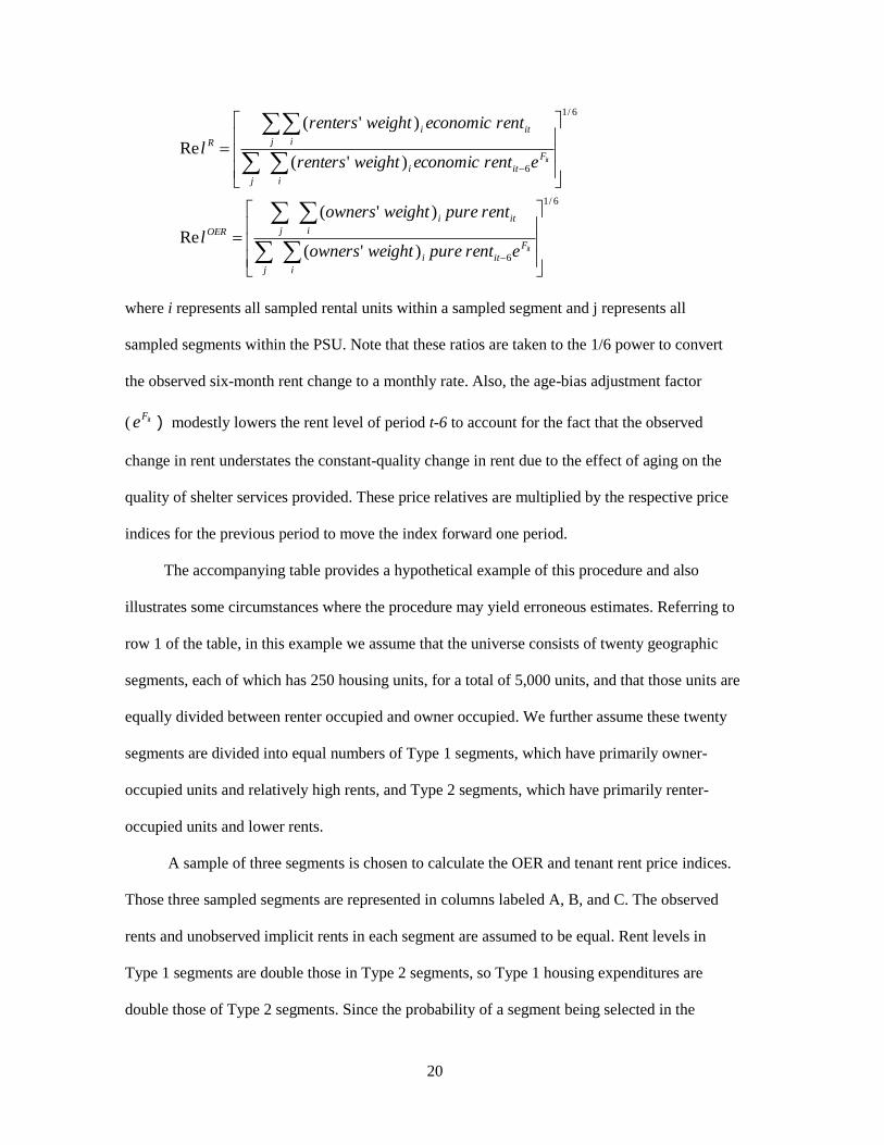
The “price relatives” for tenant rent (RelR) and for OER (Rel
OER) are then given by the
following:
20
6/1
6
6/1
6
)'(
)'(
Re
)'(
)'(
Re
i
F
iti
j
i
iti
jOER
i
F
iti
j
j i
iti
R
it
it
erentpureweightowners
rentpureweightowners
l
erenteconomicweightrenters
renteconomicweightrenters
l
where i represents all sampled rental units within a sampled segment and j represents all
sampled segments within the PSU. Note that these ratios are taken to the 1/6 power to convert
the observed six-month rent change to a monthly rate. Also, the age-bias adjustment factor
( itFe ) modestly lowers the rent level of period t-6 to account for the fact that the observed
change in rent understates the constant-quality change in rent due to the effect of aging on the
quality of shelter services provided. These price relatives are multiplied by the respective price
indices for the previous period to move the index forward one period.
The accompanying table provides a hypothetical example of this procedure and also
illustrates some circumstances where the procedure may yield erroneous estimates. Referring to
row 1 of the table, in this example we assume that the universe consists of twenty geographic
segments, each of which has 250 housing units, for a total of 5,000 units, and that those units are
equally divided between renter occupied and owner occupied. We further assume these twenty
segments are divided into equal numbers of Type 1 segments, which have primarily owner-
occupied units and relatively high rents, and Type 2 segments, which have primarily renter-
occupied units and lower rents.
A sample of three segments is chosen to calculate the OER and tenant rent price indices.
Those three sampled segments are represented in columns labeled A, B, and C. The observed
rents and unobserved implicit rents in each segment are assumed to be equal. Rent levels in
Type 1 segments are double those in Type 2 segments, so Type 1 housing expenditures are
double those of Type 2 segments. Since the probability of a segment being selected in the

21
sample depends on total housing expenditures, the sample includes two Type 1 segments and
one Type 2 segment to reflect the higher expenditures in the Type 1 segments. A segment’s
housing expenditures divided by the total housing expenditures of the universe determines that
segment’s probability of selection (row 2), and the inverse of that probability is the segment’s
weight (row 3).
We further assume that a sample of twenty-five housing units is selected from each of the
three segments drawn into the sample (row 4). Since each segment has 250 housing units, and a
sample of 25 units is drawn from each segment, the ratio HU/SU is equal to 10 for each segment
(row 5). The final set of weights is the renters’ share and the owners’ share of total housing
expenditures in each of the sampled segments (rows 6 and 7).
With the weights established, we turn to the computation of the price relatives for tenant
rent and OER. To do that, we assume that, from period 1 to period 2, observed tenant rents in all
Type 1 segments increase 4 percent while in all Type 2 segments tenant rents increase 2 percent.
We also assume in this example that unobserved owner-equivalent rents in each segment rise by
the same percentage as observed tenant rents. Under those assumptions, the increase in tenant
rent in the entire universe is 3.14 percent (row 8) while the increase in OER in the entire
universe is 3.5 percent (row 9).
Under the long list of assumptions for this example, the estimated increases in tenant rent
and OER produced by the sample of three segments are equal to the actual increases for the
entire universe. To derive the sample base tenant rent for Segment A, we multiply the base rent
of a renter unit ($400) times the renters’ weight given by the segment weight (15, from row 3)
times the ratio of total units over sampled units (10, from row 5) times the renters’ share of total
segment housing expenditures (0.4, from row 7), which equals 60, for a total of $24,000. We do
this for segments B and C, and then take the sum, deriving the sample total of housing
expenditures in period 1. We then make the same calculations for period 2, with the assumption
that rents rose 4 percent in Type 1 segments and 2 percent in Type 2 segments.

22
Of course, whenever estimates are derived from a sample there is the risk of sample bias.
But beyond sample bias, this example illustrates situations where the estimated price changes
may differ from the true ones. Key potential sources of error lie in two areas. First, the level of
OER in the base period is estimated as a nonlinear function of property value, derived from data
on tenant rents and property values in census blocks. Errors in the estimation of the OER level
would result in incorrect renters’ and owners’ weights and produce errors in both price series.
Second, the true rate of change in OER in a segment may not be the same as the observed rate of
change in tenant rents in that segment, resulting in errors in the estimated change in OER. Both
of these potential sources of error are more likely to occur in areas with relatively few rental
units.
a This is a technical change introduced in 1999. During the 1983-87 period, this segment weight was
based on the number of housing units rather than total housing expenditures. In practice, implicit rents
in a segment are estimated using a nonlinear regression relating rents in census blocks within a
metropolitan statistical area with home values.

23
REFERENCES
Armknecht, Paul A., Brent R. Moulton, and Kenneth J. Stewart. 1995. “Improvements to the
Food at Home, Shelter, and Prescription Drug Indices in the U.S. Consumer Price Index.”
Bureau of Labor Statistics Working Paper no. 263.
Billor, Nedret, Ali S. Hadi, and Paul F. Velleman. 2000. “BACON: Blocked Adaptive
Computationally Efficient Outlier Nominators.” Computational Statistics and Data Analysis 34,
no. 3: 279-98.
Bryan, Michael F., and Stephen G. Cecchetti. 1994. “Measuring Core Inflation.” In N. Gregory
Mankiw, ed., Monetary Policy. NBER Studies in Business Cycles, Vol. 29, 195-215. Chicago:
University of Chicago Press.
Bryan, Michael F., Stephen G. Cecchetti, and Rodney L. Wiggins II. 1997. “Efficient Inflation
Estimation.” NBER Working Paper no. 7479.
Cecchetti, Stephen. 2007. “Housing in Inflation Measurement.” VOX 13.
Crone, Theodore M., Leonard I. Nakamura, and Richard Voith. 2001. “Measuring American
Rents: A Revisionist History.” Federal Reserve Bank of Philadelphia Working Paper no. 01-8.
DiPasquale, Denise, and William C. Wheaton. 1994. “Housing Market Dynamics and the Future
of Housing Prices.” Journal of Urban Economics 35, no. 1 (January): 1-27.
Dougherty, Ann, and Robert Van Order. 1982. “Inflation, Housing Costs, and the Consumer
Price Index.” American Economic Review 72, no. 1 (March): 154-64.
Epstein, Gene. 2000. “Inflation’s Upward Creep Would Look Even Worse if BLS Counted
What’s Really Happening to Housing.” Barron’s, March 20, p. 40.

24
Gallin, Joshua, and Randal Verbrugge. 2007. “Improving the CPI’s Age-Bias Adjustment:
Leverage, Disaggregation and Model Average.” BLS Working Papers, #411, U.S. Department
of Labor, Bureau of Labor Statistics, Office of Prices and Living Conditions, October.
Gillingham, Robert. 1983. “Measuring the Cost of Shelter for Homeowners: Theoretical and
Empirical Considerations.” Review of Economics and Statistics 65, no. 2 (May): 254-65.
Lane, Walter, and Mary Lynn Schmidt. 2006. “Comparing U.S. and European Inflation: The CPI
and the HICP.” Monthly Labor Review (May): 20-27.
Mankiw, N. Gregory, and David N. Weil. 1989. “The Baby Boom, the Baby Bust, and the
Housing Market.” Regional Science and Urban Economics 19, no. 2 (May): 235-58.
Moulton, Brent R. 1997. “Issues in Measuring Price Changes for Rent of Shelter.” Paper
presented at the conference “Service Sector Productivity and the Productivity Paradox.” Ottawa:
Centre for the Study of Living Standards.
Poole, Robert, Frank Ptacek, and Randal Verbrugge. 2005. “Treatment of Owner-Occupied
Housing in the CPI.” Bureau of Labor Statistics, U.S. Department of Labor.
Poterba, James M. 1984. “Tax Subsidies to Owner-Occupied Housing: An Asset-Market
Approach.” Quarterly Journal of Economics 99, no. 4: 729-52.
Ptacek, Frank, and Robert M. Baskin. 1996. “Revision of the CPI Housing Sample and
Estimators.” Monthly Labor Review 119, no. 12 (December): 31-9.
U.S. Department of Commerce, Bureau of Economic Analysis. 2014. “Concepts and Methods of
the U.S. National Income and Product Accounts.”
U.S. Census Bureau. 1999. “Current Construction Reports— Characteristics of New Housing:
1998, C25/98-A.” Washington, D.C.: U.S. Department of Commerce.
———. 2000. “Current Construction Reports—Housing Completions: December 1999, C22/99-
12.” Washington, D.C.: U.S. Department of Commerce.

25
U.S. Department of Labor. 1996. “How the Consumer Price Index Measures Homeowners’
Costs.” Fact Sheet no. BLS 96-6. Washington, D.C.: Bureau of Labor Statistics.
———. 1999. “Consumer Price Indices for Rent and Rental Equivalence.” Fact Sheet no. BLS
99-4. Washington, D.C.: Bureau of Labor Statistics.
Verbrugge, Randal. 2006. “The Puzzling Divergence of Rents and User Costs, 1980-2004.”
Unpublished paper, Bureau of Labor Statistics, May.
26
ENDNOTES
1 The CPI in this case is the CPI-U, or consumer price index for all urban consumers, which
excludes farm dwellings. The weights of OER and tenant rent in the CPI are based on the
Consumer Expenditure Survey. To determine the OER weight, the survey asks homeowners to
estimate what their homes would rent for, excluding utilities and furnishings. Weights for OER
and tenant rent in the PCE deflator, while large, are lower than the corresponding weights in the
CPI due to the broader concept of consumption covered by the PCE deflator.
2 Technically, in the National Income and Product Accounts, owner-occupants are regarded as
owners of unincorporated enterprises that provide housing services to themselves in the form of
the rental value of their dwellings. See Bureau of Economic Analysis, Concepts and Methods of
the U.S. National Income and Product Accounts, Chapter 5, Personal Consumption
Expenditures.
3 Also included within the shelter component of the CPI are lodging away from home and
tenants’ and household insurance. In the case of the CPI, lodging away from home includes
hotels and motels as well as housing at school. Prior to 2010, the CPI lodging away from home
included second homes, but that component was moved into OER beginning in 2010. That
change made the treatment of second homes comparable to that of the PCE deflator. Finally,
note that for the PCE deflator, the services of hotels and motels are not included in housing but
rather are included in the food services and accommodations category.
4 This section draws heavily on several BLS publications, including U.S. Department of Labor
(1996, 1999), Ptacek and Baskin (1996), and Poole, Ptacek, and Verbrugge (2005).
5 See U.S. Bureau of Labor Statistics, Consumer Price Index, Consumer Price Indices for Rent
and Rental Equivalence, February 9, 2007, and “Updating the Rent Sample for the CPI Housing
Survey,” Monthly Labor Review, August 2013.
6 In the Consumer Expenditure Survey, homeowners are asked to estimate the current value of
their home and also what it would rent for.
7 The cost of utilities not included in contract rents is reflected in the fuels and utilities
subcomponent of the overall housing category of the CPI. The BEA specifically strips out the
influence of utilities from the BLS tenant rent measure when constructing the price index for
tenant rent within the PCE deflator. However, the BEA includes in tenant rent any major
expenditures made by the tenant for maintenance and repairs for which the landlord provides no
reimbursement.
8 These characteristics include the number of bedrooms, bathrooms, and other rooms in the unit,
utilities and facilities provided, and the type of energy used for heating and cooling.
9 Gallin and Verbrugge (2007) discuss the age-bias adjustment in detail and present alternative
methods of estimating it.
27
10
The BLS provided to us the annual average of the monthly values of the ABA that it uses. We
took the average of those values for year t and t+1 raised to the 24th power to account for the fact
that we are measuring rent changes over two-year intervals.
11
The variable also includes, in a small number of cases, the cost of renter’s insurance.
12
In our preliminary analysis, we included the squared value of the log level of housing costs as
an explanatory variable to test for nonlinearity, but it was statistically insignificant with a
negative sign and thus was not included in our final regression.
13
Trimming of the tails was performed using the BACON algorithm (see Billor, Hadi, and
Velleman [2000]). In our analysis, outliers were determined at the 5 percent level based on an
observation’s reported rental growth and reported rent level in the first two years of the panel,
with an average of 30 observations removed in a given year.
14
Crone, Nakamura, and Voith (2001) also develop an alternative tenant rent series using AHS
data. Although the period of their study mostly precedes ours, the first three panels of our study
overlap with theirs. Their alternative series also suggests a higher rate of tenant rent inflation
than is reported in the CPI.
15 The main purpose of the Consumer Expenditure Survey is to derive weights for the Consumer
Price Index. The estimate of what it would cost to rent someone’s home is the basis for the
weight assigned to OER.
16
The density functions in Chart 6 are smoothed versions of the empirical distribution, using a
normal kernel with a bandwidth parameter of 100 for renters and 300 for owners.
17
The European Harmonized Index of Consumer Prices (HICP) does not include OER. The
reason cited is that measurement is difficult and controversial. See Lane and Schmidt (2006).
18 Given the housing boom and bust of the 2000s and the ensuing financial crisis and recession,
some analysts have argued that home prices should be included in a measure of inflation used to
guide the setting of monetary policy.
19 See Cecchetti (2007) for additional discussion of this issue.
20 See, for example, the discussion in Gillingham (1983).
21 See, for example, the following blog post: http://www.doctorhousingbubble.com/housing-cpi-
lottery-how-cpi-understates-housing-inflation-los-angeles-housing-costs/.
22
Theoretically, another option for measuring the implicit rent of owner-occupied housing is to
calculate its user cost (for example, see Dougherty and Van Order [1982]). At the time the BLS
adopted the rental equivalence approach, it suggested that rental equivalence was a way of
measuring user cost more efficiently (see Gillingham [1983]). More recently, Verbrugge (2006)
examined the relationship between an estimate of user costs and rents and found that, despite the
theoretical relationship between the two, they behave very differently over long periods of time.
28
23
In 1995, the BLS made some technical changes to the split-sample approach. It changed the
formula that was used to compute the percentage change of OER (the Sauerbeck formula) to
eliminate “chain drift.” This change is estimated to have reduced the OER inflation rate by about
0.4 percentage point. In addition, the BLS began basing changes in OER (and in tenant rent) on
six-month rent changes only, rather than on the weighted average of one-month and six-month
rent changes. For further details, see Armknecht, Moulton, and Stewart (1995).
24
“Research performed by the BLS using 1980 and 1990 census data indicates that geographic
location is the most important variable…in determining rent change. Once geography is taken
into account, only rent level is significant in predicting rent change” (Ptacek and Baskin [1996]).