1

The Measurement of Inequality of Opportunity:

Theory and an application to Latin America

Francisco H. G. Ferreira and Jérémie Gignoux

August 21st, 2009

Keywords: Inequality of opportunity; Latin America

JEL Codes: D31, D63, J62.

Abstract: This paper proposes two simple scalar measures of inequality of

opportunity: inequality measured in the “smoothed distribution”

corresponding to a given partition of the population into circumstance-

homogeneous types (IOL), and the ratio of that quantity to overall

inequality in the original distribution (IOR). Both measures are derived

from a weak definition of equality of opportunity which must necessarily

hold under Roemer‟s stronger criterion. Alternative parametric and non-

parametric estimation methods are proposed, both of which yield lower-

bound estimates of inequality of opportunity. In an application to six

countries in Latin America, we find inequality of opportunity shares (IOR)

ranging from one quarter to one half of total consumption inequality. An

opportunity-deprivation profile that identifies the worst-off types in each

society is also formally defined, and applied to the same six countries. In

three of these six countries, 100% of the opportunity-deprived were found

to be indigenous or Afro-descendents.

Development Research Group, the World Bank. We are grateful to Caridad Araujo, Pranab Bardhan,

Ricardo Paes de Barros, Marc Fleurbaey, James Foster, Markus Goldstein, Peter Lanjouw, Marta

Menéndez, John Roemer and Jaime Saavedra for helpful comments on earlier drafts. Insightful comments

were also received at conferences or seminars at the World Bank, the IDB, the Brookings Institution, the

Catholic University of Milan, Universidad de los Andes in Bogotá, Colégio de México, Universidad

Torcuato di Tella in Buenos Aires, and the Universities of London, Lund, Manchester and Oxford. We also

thank Carlos Becerra, Jofre Calderón, and Leo Gasparini, for kindly providing us with access to data. The

views expressed in the paper are those of the authors, and should not be attributed to the World Bank, their

Executive Directors, or the countries they represent. Correspondence to fferreira@worldbank.org and

jgignoux@worldbank.org.

2

1. Introduction

Economic inequality – usually measured in terms of income or consumption – is

neither all bad nor all good. Most people view income gaps that arise from the application

of different levels of effort as less objectionable than those that are due, say, to racial

discrimination.1 Indeed, the distinction between inequalities due to the exercise of

individual responsibility on the one hand, and those due to morally irrelevant pre-

determined circumstances on the other, has become central to the literature on social

justice in political philosophy, social choice and, increasingly, in mainstream economics.

Dworkin (1981), Arneson (1989), Cohen (1989) and, to some extent, Sen (1985)

are among a number of influential authors to have argued that inequality in the

distribution of particular outcomes – such as incomes – is not the appropriate yardstick

for assessing the fairness of a given allocation or social system. Despite important

differences in nuance, these authors have all suggested that some outcome differences -

which are attributable to differences in choices for which individuals can be held

responsible – may be ethically acceptable. In this view, unacceptable inequalities reside

in a logically prior space – of resources, capabilities, opportunities – for which

individuals cannot be held responsible.2

John Roemer (1998), for instance, calls those factors over which individuals have

a measure of control “efforts” (e.g. how long one studies, or how hard one works), while

those for which they cannot reasonably be held to have any responsibility are referred to

as “circumstances” (e.g. race, gender or family background). Given this distinction, he

1 Attitudinal surveys attest to this. When asked to place their views on a scale from 1 to 10, where 1 implied

agreement with the statement that “Incomes should be made more equal”, and 10 implied agreement with

the statement that “We need larger income differences as incentives for individual effort”, respondents in

the 1999-2000 wave of the World Value Survey (fielded in 69 countries) were evenly divided. The median

answer was 6. The two modes of the distribution, with approximately 20% of respondents each, were 1 and

10. 2 Space constraints prevent us from exploring these differences in nuance here. They may well be

philosophically important, and have been reviewed extensively elsewhere (see, e.g. Roemer, 1993a). The

point here is simply that all of these approaches contributed to a shift away from seeking equality in

outcomes, and towards assessing social justice with respect to a “prior” space of enabling conditions faced

by individuals, while according an ethically acceptable role to individual responsibility and its

consequences.

3

defines “equality of opportunity” essentially as a situation in which important outcomes –

which he calls “advantages” – are distributed independently of circumstances.3

Such a distinction between inequality of opportunity and the more standard

concept of inequality of outcomes is of interest to economists for at least three sets of

reasons. First, there is an increasingly widespread normative view that it is inequality of

opportunity, and not that of outcomes, which should inform the design of public policy.

Inequality of opportunity is, in this view, the appropriate “currency of egalitarian justice”

(Cohen, 1989). Public action need not necessarily aim to eliminate all outcome

inequalities, but may be justified in seeking to reduce those that arise from unequal

opportunities: “economic inequalities due to factors beyond the individual responsibility

are inequitable, and should be compensated by society” (Peragine, 2004, p.11). To the

extent that this view, which is already popular among social choice theorists and political

philosophers, gains traction among policymakers, it will behoove economists to provide

tractable empirical measures of the concept.

Second, if inequality of opportunity affects popular attitudes to outcome

inequality, then it may affect beliefs about social fairness and attitudes to redistribution.

These beliefs and attitudes may in turn affect the extent of redistribution actually

implemented in society, and thus the level of investment and output generated. It has

often been argued, for instance, that one source of difference between the attitudes of

Americans and Europeans to inequality is that the former tend to believe that “society is

mobile and one can escape poverty with hard work” (Alesina et al, 2004, p.2011), while

the latter feel that individual choices are less powerful than predetermined circumstances

in determining their relative positions in the distribution. Such beliefs are of interest to

economists regardless of their accuracy: Alesina and Angeletos (2005) and Bénabou and

Tirole (2006) provide examples of models where such beliefs and attitudes themselves

play a key role in generating multiple equilibria, with very different objective economic

characteristics.

3 Roemer phrases his definition somewhat differently. He argues that, if it were possible to partition the

population into circumstance-homogeneous groups (which he calls “types”), and if the only variable that

differed across individuals within each type was their effort level, then equality of opportunity would attain

only if the distributions of advantage across all such groups were identical. Under Roemer‟s assumptions,

the requirement of identical distributions of advantage regardless of type is equivalent to stochastic

independence between advantage and circumstances. Although this should be intuitively clear, we return to

this argument more formally in Section 2.

4

Third, it has also been suggested that inequality of opportunity might be a more

relevant concept (than income inequality) for understanding whether aggregate economic

performance is worse in more unequal societies (and if so, why). In addition to the role of

beliefs and attitudes to redistribution, it is possible that the kinds of inequality that are

detrimental to growth (such as inequality in access to good schools, or to financial

markets) are more closely associated with the concept of opportunities, while other

components of outcome inequality – such as those arising from differential returns to

effort – may actually have a positive effect on growth (World Bank, 2006; Bourguignon,

Ferreira and Walton, 2007). Perhaps one of the reasons why the cross-country empirical

literature on inequality and growth is so inconclusive is that it conflates the two kinds of

inequality.4 In fact, a recent study by Marrero and Rodriguez (2009) finds that if one

decomposes total income inequality into an “opportunity” component and an “effort”

component, both terms have statistically significant coefficients in a growth regression

estimated for 23 states of the United States in the last two decades. But while the

coefficient on inequality of opportunity has a negative sign, the opposite is true for

inequality of efforts.

In order to make empirical use of the concept of inequality of opportunity,

however, whether in the design of taxation and public expenditures or in the study of the

determinants of cross-country growth differences, it is first necessary to measure it

appropriately. This is the intended contribution of this paper. It proposes two simple (and

closely interrelated) measures of inequality of opportunity, which are based on a

reinterpretation of the standard decomposition of inequality indices by population

subgroups: one is an “inequality of opportunity level” (IOL) measure, while the other is

an “inequality of opportunity ratio” (IOR). We provide a firm theoretical foundation for

the measures by deriving them explicitly from the pioneering definitions of equality of

opportunity due to Roemer (1993b, 1998) and van de Gaer (1993). We draw on the

theory of path-independent decomposability of Foster and Shneyerov (2000) to eliminate

index-ambiguity, and to anchor our measures to a single, most-appropriate inequality

index: the mean logarithmic deviation.

4 See Banerjee and Duflo (2003) on the inconclusiveness of that literature.

5

In order to enhance their practical usefulness in the real world of finite sample

sizes, we propose two alternative estimation procedures for our indices of inequality of

opportunity: a non-parametric and a parametric method. In applications to six countries in

Latin America - Brazil, Colombia, Ecuador, Guatemala, Panama, and Peru – we show

that the two methods tend to generate robustly similar results for large samples, but that

the parametric approach yields more conservative estimates of the lower-bound for

inequality of opportunity in smaller samples.

The combination of robust estimation procedures and reasonably rich data sets

allows us to use a larger set of circumstance variables than the previous literature. This

contributes to lower-bound estimates of the inequality of opportunity ratio (IOR) ranging

from 24% of total inequality in household consumption in Colombia, to 50% in

Guatemala.

Finally, we propose a ranking of types within society which is of direct practical

relevance for implementation of the concepts of “equal opportunity policy” found in the

literature, and to Roemer‟s proposed criterion for assessing economic development.5 We

define both an opportunity profile and an opportunity-deprivation profile, and illustrate

them for our Latin American sample, where we find that rankings vary substantially

across countries (with ethnicity being fundamental in Brazil but much less important in

Colombia, for instance). Because the empirical approach proposed here is: (i) well

grounded in the theory of inequality of opportunities, (ii) extremely simple

computationally, and (iii) capable of handling a large number of types (relative to

alternative approaches), we hope that it will contribute to further progress in empirical

work on the causes and consequences of inequality of opportunity.

The remainder of the paper is structured as follows. Section 2 derives our basic

indices from the theory of equal opportunities, and relates them to the existing literature

on the measurement of inequality of opportunity. Section 3 discusses two alternative

procedures for estimating the indices in practice: a non-parametric approach that has the

advantage of flexibility, and a parametric approach that may be more suitable when the

sample size is small. Section 4 provides some information on the six household survey

5 Roemer (2006) suggested that “the rate of economic development should be taken to be the rate at which

the mean advantage level of the worst-off types grows over time.” (p.243).

6

data sets used in our empirical application. Section 5 presents the empirical results and

Section 6 discusses the opportunity and opportunity-deprivation profiles for all six

countries. Section 7 concludes.

2. A conceptual framework

Consider a finite population of discrete agents indexed by Ni ,...1 , where N is

large. Each individual i is characterized by a set of attributes iii eCy ,, , where y denotes

an advantage, C denotes a vector of circumstance characteristics, and e denotes an effort

level. We follow Roemer (1998) in considering a single advantage variable (which we

will later associate with household per capita income or consumption), and in

representing effort as a scalar.6 We will also follow Roemer (1998) in treating effort as a

continuous variable, while the vector Ci consists of J elements corresponding to each

circumstance j (for individual i), with the typical entry being j

iC . Furthermore, each

element j

iC takes a finite number of values, xj, i .7

This permits us to partition the population into Roemerian types, i.e. population

subgroups that are homogeneous in terms of circumstances. This partition is given by

KTTT ,...,, 21 , such that NTTT K ,...,1...21 , klTT kl ,, , and the

vectors .,,,, kTjTijiCC kkji Naturally, the maximum possible number of

types is given by

J

j

jxK1

.8 It will prove useful to denote the joint distribution of

advantages and circumstances over the population by {y, C}, and the space of such

distributions by Ω. The marginal distribution of advantages, of course, is given simply by

the vector y = Nyy ,...,1 Similarly, denote the space of possible population partitions Π

by Λ.

6 We later show that the proposed indices do not hinge on effort being a scalar, and are perfectly consistent

with some alternative representation, such as a vector of efforts, E. 7 For clarity, subscripts applied to C denote individuals, while superscripts denote elements in the C vector.

While our treatment of circumstances as discrete variables is common to most of the literature, see O‟Neill

et al. (2000) for an alternative approach that relies on a single continuous circumstance variable. 8 KK if some cells in the partition are empty in the population.

7

In his original formal definition of equality of opportunity, Roemer (1998) defines

the distribution of effort within each type Tk, eG k

as “a probability measure on the set

of effort levels, which are non-negative real numbers” (p.10). Since he is primarily

concerned with defining an equal-opportunity policy, or set of allocation rules, he adds a

subscript to indicate that the distribution of efforts is conditional on some policy ρ. He

denotes the advantage level enjoyed by a person in quantile eG k

of the effort

distribution in type k, given policy ρ, as ,ky . His analysis is then couched in terms of

seeking an equal-opportunity policy ρ*, which he ultimately proposes should maximize

the average (over quantiles of the effort distribution) of minimum levels of advantage

across all types, at each given quantile:

1

0

,minmaxarg*

dy k

k (1)

Although Roemer (1998) does not actually write down a formal definition of

equality of opportunity itself – only that of the equal opportunity policy – his equation (1)

has been widely interpreted to imply that equal opportunities would arise if the levels of

advantage were the same for each quantile of the effort distribution, across types (for

some given policy ρ):

lk

lk TTyy ,;1,0,,, . (2)

Equation (2) clearly accords with Roemer‟s informal statement that “leveling the

playing field means guaranteeing that those who apply equal degrees of effort end up

with equal achievement, regardless of their circumstances. The centile of the effort

distribution of one‟s type provides a meaningful intertype comparison of the degree of

effort expended in the sense that the level of effort does not” (1998, p.12, emphasis

added).9

Now denote the cumulative distribution function of advantage in type k, under

policy ρ, by yF k

. Note that the effort rank (π) and the advantage rank must be the same

9 Equalizing advantages across types for each quantile, rather than level, of effort is justified by what

Roemer calls his “assumption of charity”. Since circumstances also affect efforts, the effort distribution

within each type is itself a characteristic of the type. The assumption of charity states that “within any type,

that distribution would be the same, if we were able to factor out the (different) circumstances which define

different types” (Roemer, 1998, p.15)

8

within each type because, given circumstances, advantage is fully and monotonically

determined by effort. Dropping the policy subscript ρ, which is not the focus of our

analysis, and noting that ky is simply the inverse function of yF k , (2) then

implies:

lk

lk TTklyFyF ,,, (3)

This is presented as Roemer‟s “strong criterion” definition of equal opportunities

in Bourguignon, Ferreira and Walton (2007), and by Lefranc, Pistolesi and Trannoy

(2008).10

If equality of opportunity corresponds to a situation in which advantage

distributions are identical across types, then the measurement of inequality of opportunity

must, in some sense, seek to capture the extent to which yFyF lk , for lk . An

obvious first step would be to test for the existence of inequality of opportunity, by

examining whether the conditional distributions of advantage differ across types. This is

precisely what Lefranc et al. (2008) do, using stochastic dominance concepts and the

associated statistical tests to compare the distribution of opportunities across types in a

number of OECD countries, where the types are defined by the level of education (or, in

a couple of cases, occupation) of a person‟s father.11

Theirs is a very interesting approach to ascertaining whether or not individual

countries could be described as having equality of opportunity (in their sample, the null

hypothesis of equal opportunities can be rejected for every country, except Sweden). It

also allows for a (partial) ranking of types within each country, relying on the dominance

comparisons. This partial ranking is complemented by a scalar index for inequality of

opportunity, which is based on a variant of the Gini coefficient, defined over mean

10

Lefranc et al. (2008) refer to equation (3) - albeit obviously in slightly different notation – as “a

compelling case of equality of opportunity [that] corresponds to the definition of equality of opportunity

adopted by Roemer (1998).” (p.517). Similarly, if circumstances and advantages were alternatively defined

as continuous variables, the joint distribution of which was given by Cy, , and where the

corresponding conditional distribution were given by CyF , then the corresponding definition would be

yFCyF . See the working paper version of this paper: Ferreira and Gignoux (2008).

11 See also Hild and Voorhoeve (2004) on the philosophical implications of using stochastic dominance

criteria for evaluating the extent of inequality of opportunity.

9

advantage levels for each type and adjusted for “within-type inequality”. See Lefranc et

al. (2008).

However, while this reliance on stochastic dominance comparisons across type-

specific advantage distributions is desirable in terms of robustness, it does come at a

practical cost, given usual sample sizes. Because the estimation of distribution functions

(or Generalized Lorenz curves) requires a reasonable number of observations within each

type, the partition Π of the population must perforce be quite coarse. Lefranc et al. (2008)

work with K = 3 in all countries. This implies a rather limited treatment of inequality of

opportunity, since any inequality within those three types is then associated with

differences in efforts. These would include, for instance, any income differences

associated with gender, race or birthplace that might exist within types defined solely on

the basis of father‟s education. It is not obvious whether the Gini of Opportunity ranking

in Lefranc et al. would remain unchanged if, for instance, inequalities across different

racial groups were taken into account, say in the US and Italy.

An alternative approach, which we pursue here, is to adopt a weaker equality of

opportunity criterion, which is necessary but not sufficient for (3), namely that mean

advantage levels should be identical across types. If we define

0

yydFy kk , then

this weaker criterion for equality of opportunity is written:12

lk

lk TTklyy ,,, (4)

Adopting this weaker definition of equal opportunities, the measurement of

inequality of opportunity must now seek to capture the extent to which yy lk ,

for lk . This seems an easier task, since it appears to call for an inequality index

defined not on the marginal distribution of advantages, y = Nyy ,...,1 , but on the

corresponding smoothed distribution.

12

Interestingly, this weaker equal-opportunity criterion is related to an early debate in the

conceptual literature on equal-opportunity policies. In that context, Roemer (1993b) proposed taking the

minimum (across types) at each centile of the conditional distribution of advantages, and then averaging

across centiles (Equation 1), in the so-called “mean of mins” approach. Alternatively, van de Gaer (1993)

proposed first averaging across centiles, and then taking the minimum across types (a “min of means”):

kk

k

k

kVDG ydy

minmaxarg,minmaxarg*

1

0

10

A smoothed distribution, which we denote k

i , was originally defined by Foster

and Shneyerov (2000), drawing on the earlier inequality decomposition literature

associated with Bourguignon (1979), Cowell (1980) and Shorrocks (1980). It has been

applied to the measurement of inequality of opportunity by Checchi and Peragine (2005).

The smoothed distribution k

i is obtained from a distribution of advantages y and a

partition Π by replacing each individual advantage k

iy with the group-specific mean,

yk .

The weak criterion of equality of opportunity in (4) and the definition of a

smoothed distribution immediately give rise to two candidate scalar measures of

inequality of opportunity, which map from a joint distribution of advantage and

circumstances {y, C} and from the associated partition Π, to the non-negative real line.

These are given by .: :13

k

ia I (5)

and yI

I k

ir

(6)

θa is a measure of the absolute level of inequality of opportunity (IOL), while θr

measures that level in relation to total inequality, and is thus an inequality of opportunity

ratio (IOR). I() is any index that satisfies the axiomatic properties which are now standard

in the literature on the measurement of relative inequality (see, e.g. Cowell, 1995). These

properties include symmetry (or anonymity); the transfer principle; scale invariance;

population replication and, crucially, additive decomposability. This last property

requires that k

kk

k

i yIwIyI , where yk denotes the income vector within each

type Tk, and wk denotes type-specific weights, subject to 1k

kw .14

13

θr is actually a mapping 1,0: , 14

The treatment of effort as a continuous variable, and the ensuing notation with continuous within-type

distributions Gk(e) and F

k(y), were useful primarily to relate our conceptual framework to the existing

theory of equality of opportunity (in particular to Roemer, 1998). From this point onwards, with effort only

in the background of the analysis, we revert to a fully discrete notation, and use yk as the within-type

income vector. There is no other change in notation, and the marginal and joint distributions of advantage

and circumstances defined earlier are unchanged.

11

For any inequality index I() that satisfies these properties, it is easy to check that

both θa and θr satisfy:

(i) Principle of population: the index is invariant to a replication of the

population N,...,1 .

(ii) Scale invariance: the index is invariant to the multiplication of all

advantages by a positive scalar.

(iii) Normalization: if the smoothed distribution k

i is degenerate, so that

equation (4) holds, then the index must take a value of zero.

(iv) Within-type symmetry: the index is invariant to any permutation of two

individuals within a type.

Furthermore, the IOL measure θa satisfies:

(v) Within-type transfer insensitivity: the index is invariant to any mean-

preserving spread in advantages within a type.

(vi) Between-type transfer principle: the index weakly rises with any transfer

from any individual i to j, if lk TjTi , , with lk .

The class of indices I() that satisfy symmetry (or anonymity), the Pigou-Dalton

transfer principle, scale invariance, population replication and additive decomposability

reduces to a well-known class of inequality measures. Shorrocks (1980) and Foster

(1985) show that (under a regularity condition) an inequality measure satisfies the four

basic properties and additive decomposability if and only if it is a positive multiple of a

member of the Generalized Entropy (Eα) class.

Nevertheless, that is still a large class of measures. As is well known, an

inequality decomposition by population subgroup, for a given distribution of advantages

and for a given partition, will in general differ for different indices I() in the Generalized

Entropy family, implying that θa and θr are not uniquely defined. So, for a given

smoothed distribution – that is, for a given joint distribution {y, C} and partition Π – one

could obtain different values for each of our inequality of opportunity indices, by

selecting different inequality measures I() from the set of indices that satisfies the

previously imposed axioms. Since these measures are sensitive to different parts of the

12

distribution, different choices of I() could in principle lead to different rankings across

two smoothed distributions.

Fortunately, there is an eminently plausible further requirement which allows us

to refine the set of eligible indices to a singleton, namely Foster and Shneyerov‟s (2000)

path-independent decomposability axiom. Just as we previously defined a smoothed

distribution, now define a standardized distribution, denoted k

i , as the distribution

which is obtained from a distribution of advantages y and a partition Π, by replacing k

iy

with k

k

iy

(where μ is the grand mean). Just as a smoothed distribution eliminates all

within-group inequality by construction, a standardized distribution eliminates all

between-group inequality, by appropriately rescaling all subgroup means. One might

therefore wish to impose the requirement that k

i

k

i IyII . This requirement

is the axiom of path-independent decomposability.

Foster and Shneyerov (2000) fully characterize the “path-independent

decomposable” class of inequality measures. They show that when the set of inequality

indices I() under consideration is restricted to those that use the arithmetic mean as the

reference income, and that satisfy the Pigou-Dalton transfer axiom, this class reduces to a

single inequality measure, the mean logarithmic deviation, which we will denote E0 since

it is a member of the generalized entropy class of measures, when its parameter is set to

zero.15

By adding path-independent decomposability to the list of axioms that our

inequality indices I() must satisfy, we are now able to restrict our set of scalar measures

of inequality of opportunity (IOL and IOR respectively) to two unique indices:

15

It is easy to see why the two decomposition paths yield different results for other generalized entropy

measures. The decomposition of total inequality for these measures can be written as follows:

kK

k

kkk

i yEN

nEyE

1

, where nk and y

k denote, respectively, the population

and the advantage distribution in type k, and α is the generalized entropy parameter. The first term in the

right-hand side of this equation – the between-group component - is inequality in the smoothed distribution.

The second term is the within-group component. Clearly, for 0 , the rescaling of subgroup means

implied by standardization (k

k

iy

) does not only drive the first term (the between-group component) to

zero. It also affects the weights in the within-group term. So, for 0 , k

i

k

i EyEE .

13

k

ia E 0 (5‟)

and yE

E k

ir

0

0 (6‟)

These two scalar measures of inequality of opportunity have a number of

appealing features. First, they derive directly from a definition of inequality of

opportunity (in equation 4), which is implied by Roemer‟s (1998) stronger criterion (in

equation 3). Second, this weaker criterion is formally consistent with van de Gaer‟s

(1993) “min of means” approach to finding the equal opportunity policy (see footnote

12). Third, the indices satisfy a range of desirable properties, listed above as axioms (i)

through (vi) for θa (and i through iv for θr), as well as path-independence. Fourth, they are

extremely simple to calculate, and are identical to the between-group component (θa) or

share (θr) of the standard Theil-L decomposition by population subgroups, provided the

population is partitioned by circumstance variables only, as in our earlier definition of

KTTT ,...,, 21 .

Property (v), namely within-type transfer insensitivity, also sets θa apart from

other measures in current use, such as Lefranc et al.‟s Gini of Opportunities, which is

(deliberately) sensitive to “risk” - or inequality - within types. The approach here is to

take seriously the notion that the only kind of ethically objectionable inequality is that

associated with opportunities, i.e. that which occurs between types. The index is therefore

deliberately insensitive to within-group inequality. Within-type transfer insensitivity may

be seen as a kind of “focus axiom” for inequality of opportunity measurement: if types

are well-defined, so that individuals are homogeneous in circumstances within each type,

then within-group inequality should be ignored, much as incomes above the poverty line

are ignored by virtue of the focus axiom in poverty measurement.

A similar argument applies to property (vi), the between-type transfer principle,

which requires the inequality of opportunity index to rise if a transfer is made from

someone in a “poorer” type to someone else in a “richer” type – regardless of whether the

first person is individually richer or poorer than the second.

Although we find these two axioms conceptually appealing for a measure that

seeks to isolate and quantify inequality of opportunity, they do not apply to θr, which is

decreasing in within-group inequality by construction. While IOL (θa) is our “preferred”

14

index, we nevertheless define and use IOR (θr) in our empirical application below, as a

complementary measure. This is in part because we have found that expressing inequality

of opportunity as a share of total inequality in some advantage is appealing from a

communications perspective. It abstracts from the unit of measurement in the mean log

deviation, and can easily be grasped by many audiences. But it is also because there may

be certain contexts in which the share of opportunity in total inequality, rather than the

level of inequality of opportunity, is actually the primary object of interest. This may be

the case, for instance, if voters (or aid donors) decide whether or not to support a

particular redistribution policy depending on whether they perceive most inequality to be

driven by circumstances or by efforts. In that case, decisions may hinge on whether IOR

is greater or less than 0.5. Obviously, if one insists on axioms (v) and (vi), then only θa

should be used, with no reference to θr.

The indices in (5‟) and (6‟) are closely related to two earlier contributions to the

incipient literature on measuring inequality of opportunities. They are similar to the

“types approach” to inequality measurement proposed by Checchi and Peragine (2005),

who apply it to a comparison of inequality of opportunity in northern and southern Italy,

using the highest educational attainment among a person‟s parents to define the partition

into types.16

They are also similar to the regression-based approach to computing the

share of inequality of opportunity for different cohorts of workers in Brazil, by

Bourguignon, Ferreira and Menéndez (2007)17

. The relationship between our approach

and theirs is discussed in more detail in the next section, where we present the non-

parametric and parametric alternative estimation procedures for θa and θr.

3. Estimating IOL and IOR in practice.

Given a sample with information on the advantage and circumstance variables in

the joint distribution {y, C}, and agreement on a partition Π, θa and θr can be calculated

16 Checchi and Peragine (2005) also discuss an alternative “tranches approach”, based on a reweighting of

individual advantages for people who can be considered to have exerted the same degree of effort, by

occupying the same quantiles in their type-specific distributions of advantage. See Fleurbaey (2008) for a

thoughtful discussion of the ethical implications of the choosing between the types and tranches

approaches. See also van de Gaer et al. (2001) for an approach based on transition matrices. 17 See also Cogneau and Gignoux (2009).

15

immediately by any algorithm that computes

N

ik

i

k

iN

E1

0 log1

, the between-group

component in the standard decomposition of the mean logarithmic deviation by

population subgroups.

This standard non-parametric approach is certainly optimal for most common

sample sizes, provided there are relatively few types in the partition Π. It was, for

instance, the method used by Checchi and Peragine (2005), who had K=5 types. As noted

earlier, however, a small K requires assuming a very limited role for circumstances. In

both Checchi and Peragine (2005) and Lefranc et al. (2008), inequality of opportunity is

taken to be associated only with differences between 3 or 5 groups, defined by a coarse

categorization of parental background. In both cases, using the notation from Section 2,

the circumstance vector C is actually a scalar (J=1), and xj is either 3 or 5.

Such a restrictive approach to partitioning the population into types is likely to

lead to an underestimate of inequality of opportunity. Any inequality due to, say, race,

gender, birthplace, or family wealth, which may remain within those three to five types,

would be attributed to effort. As we will see in the next section, many surveys do contain

information on a number of other variables which can be unambiguously classified as

circumstances. In addition to mother‟s and father‟s education, surveys often contain

information on parental occupation, race or ethnicity, gender and place of birth. As J and

xj rise, K increases geometrically.

As the number of types increases, the frequency of sample observations per type

(or cell) tends to diminish quite rapidly. In the empirical applications that follow, with

five circumstance variables (J=5), and two or three possible values per circumstance (xj =

2 or 3), we end up with 108K . In two of our six countries, this led to there being over

a fifth of all types for which there were fewer than five observations in the sample,

causing the precision of the estimates of mean advantage per type to become

unacceptably low.

As is often the case when sample sizes are insufficient for fully flexible, non-

parametric estimation, a parametric alternative is available that permits efficient

estimation, at the cost of some functional form assumptions. This was the route followed

16

by Bourguignon, Ferreira and Menéndez (2007), although that paper did not relate its

regression-based approach to the non-parametric method discussed above.

Bourguignon, Ferreira and Menéndez (2007) note that Roemer‟s view of

advantages as determined by circumstances and efforts (plus possibly luck, or unobserved

random terms) would be consistent with a stylized model of advantage of the general

form uECfy ,, . Since circumstances are economically exogenous by definition – in

the sense that they cannot be affected by individual decisions – but given that efforts may

be, and generally are, influenced by circumstances, one would rewrite this more fully

as:18

uvCECfy ,,, . (7)

For the purpose of measuring inequality of opportunity – rather than of estimating

any causal relationship between circumstances, efforts, and advantages – one can simply

write the reduced form of (7) as ,Cy .19

If one then estimates (say, by OLS) a log-

linearized version of this equation: Cyln , one can construct a parametric

estimate of the smoothed distribution as:

ˆexp~ii C (8)

Here, a hat indicates the parameter estimate from an OLS regression, and the tilde

indicates a counterfactual advantage level. The vector ~ (whose elements are given by

(8) for each i) is a parametric analogue to the smoothed distribution k

i because, by

eliminating the residuals, (8) replaces individual advantage levels with their predictions.

Predicted advantage is, of course, the same for all individuals with identical

circumstances.

Similarly, the parametric estimate of the standardized distribution would be given

by:

iii C ˆˆexp~ (9)

18

The stochastic terms u and v can be thought to account for luck and other random factors. For an

excellent recent treatment of the role of luck in the theory of equality of opportunity, see Lefranc, Pistolesi

and Trannoy (forthcoming). In empirical applications, they will also capture variation in unobserved

determinants. 19

This is why, as noted earlier, our approach to the measurement of inequality of opportunity is perfectly

consistent with a view of efforts as a vector, E, rather than a scalar, e.

17

Here, the overbar indicates an average of circumstance across all individuals. By

assigning the vector of average circumstances to all individuals, but retaining within-type

variation (through i ), the vector ~ becomes a parametric analogue to the standardized

distribution k

i .

We can thus define parametric (smoothed) estimates for our inequality of

opportunity indices as follows:

~0Ep

a (10)

and yE

Ep

r

0

0~

(11)

Parametrically standardized estimates are obtained as:

~00 EyEPS

a (10‟)

yEEPS

r 00~1 (11‟)

Although (10) and (10‟), and (11) and (11‟), are estimates for a same path-

independent measure, the fact that they are estimated parametrically, involving linear

functional form assumptions, means they are not exactly identical. However, they are

generally very similar, and the parametric estimates for IOL and IOR that we report in

Section 5 below are obtained from the parametrically standardized distributions, through

(10‟) and (11‟), respectively.

Two important methodological considerations remain, before we can turn to the

empirical application. First is the issue of omitted circumstance variables. Realistically,

the vector C observed in a particular data set is likely to be a subset of the theoretical

vector C of all possible circumstances that help determine a person‟s advantage. A “true”

measure of inequality of opportunity, as conceptually defined in equations (5) – (6),

would require that all relevant circumstance variables, and all relevant values for these

circumstances, be used to define the partition Π. This is unlikely ever to be the case in

practice for almost any conceivable data set. It is certainly not the case for the six

countries in our application below, even though we work with a much finer partition of

circumstances than any other study we are aware of.

The implication is that the empirical estimates defined in this section – whether

parametric or non-parametric – should be interpreted as lower-bound estimates of

18

inequality of opportunity. To see why they are lower bounds, consider the following

thought exercise. Imagine that an additional circumstance, previously unobserved, now

becomes observed, raising the dimension of C from J to J+1. This causes every cell in

the partition Π to be further subdivided into xJ+1 cells), increasing the maximum number

of types, K , by a factor of exactly xJ+1. The effect of this on

N

ik

i

k

iN

E1

0 log1

cannot be negative. Observing a previously omitted circumstance variable cannot lower

the between-group inequality share and, unless the additional element is orthogonal to the

measure of advantage, will raise it. This makes all empirical estimates given by (5‟), (6‟),

(10‟) or (11‟) lower-bound estimates.20

The parametric estimates are, as noted above, merely alternative estimates for the

same quantities, which rely on linear regressions to economize on data. They are also,

necessarily, lower-bound estimates. Again, to see this, consider adding an additional

element of C to the regression Cyln . This cannot reduce – and will in general

increase – the share of variation in y which is accounted for by ˆexp~ii C .

Including previously unobserved circumstances will in general raise p

a , p

r , and their

standardized analogues. 21

The second methodological consideration worthy of note is that the parametric

approach might permit the estimation of the partial effects of one (or a subset) of the

20

A similar effect would arise from refining the partition of the population into categories within each

circumstance variable in C – i.e. increasing xj for a given J. An example from our empirical analysis below

is the classification of parental occupations into only two cells: “agricultural worker” or “other”. For most

circumstance variables, international comparability required aiming for “common denominator”, relatively

aggregated classifications. Like adding other circumstance variables, further subdivision of these categories

within each circumstance might also increase (but could not reduce) the share of inequality attributed to

opportunities. 21

It is of course possible that the share of inequality attributed to a specific set of (observed) circumstances

is overestimated – say, because a previously unobserved circumstance is negatively correlated with all

previously observed ones. But the share of inequality attributed to all circumstances (rather than to the

observed subset) cannot fall by enlarging the circumstance set. Just as in the non-parametric case, these

measures are lower-bound estimates of inequality of opportunity. This emphasis on the lower-bound

measure of the effect of all circumstances is a major departure from Bourguignon, Ferreira and Menéndez

(2007), who sought to estimate the effect of a specific, observed set of circumstances, on opportunities.

That objective required them to use Monte-Carlo simulations to estimate bounds around the possible biases

in specific coefficients. If one is interested in a lower-bound for the overall effect of all circumstances, that

procedure is entirely unnecessary.

19

circumstance variables, controlling for the others, by constructing alternative

counterfactual distributions, such as:

i

JjJj

i

JJ

i

J

i CC ˆˆexp~ (12)

in the case of a parametrically standardized decomposition. Equation (12) would permit

us to compute circumstance J-specific inequality shares, or “partial IORs”:

k

i

J

i

J

r yII ~1 (13)

However, such partial shares do rely on the validity and unbiasedness of specific

reduced-form coefficients ψ. These are not, therefore, lower-bound estimates of anything.

They are meaningful only as estimates of the (total) contribution of a particular

circumstance to inequality of opportunities under the much stronger assumption that any

circumstance variables omitted from the reduced-form regression Cyln are

orthogonal to C. While we report some of the partial shares given by (13) in Section 5,

we do not insist much on them, given their strong assumption requirements.

We now apply this approach to measuring inequality of opportunity for household

welfare in six Latin American countries. For each country, we report - and compare -

both non-parametric (equations 5‟ and 6‟) and parametric estimates (equations 10‟ and

11‟) for IOL and IOR. We also report some partial shares for individual circumstances,

subject to the caveat discussed immediately above. Before presenting the results in

Sections 5, however, the next section briefly describes the data sets.

4. The data

We use data from six nationally representative household surveys in Latin

America, namely the Brazilian Pesquisa Nacional por Amostra de Domicílios (PNAD)

1996; the Colombian Encuesta de Calidad de Vida (ECV) 2003; the Ecuadorian Encuesta

Condiciones de Vida (ECV) 2006; the Guatemalan Encuesta Nacional sobre Condiciones

de Vida (ENCOVI) 2000; the Panamanian Encuesta de Niveles de Vida (ENV) 2003; and

the Peruvian Encuesta Nacional de Hogares (ENAHO) 2001. This particular group of

surveys was selected for containing information on family background for adult

individuals, such as their parents‟ education levels, father‟s occupation, or both.

20

In all countries, we restrict the sample to households containing individuals aged

30 to 49, which are the cohorts with the highest proportion of employed persons. For

Brazil and Peru, we further restrict the sample to household heads and their spouses, as

the family background information was collected only for these individuals. Sample sizes

for each survey, both before and after excluding observations with missing data, are

reported in Table 1. Sample sizes with complete information range from about 6,000 (for

Panama) to 72,000 observations (for Brazil).

Household wellbeing, proxied by household per capita income (and consumption

expenditure, where available) is used as our measure of advantage (y).22

Household

incomes are computed as the sum of all household members‟ individual incomes, and

include earnings from all jobs, plus all other reported incomes, such as those from assets,

pensions and transfers.23

Consumption expenditure data is not available for Brazil.

Elsewhere, the reference period is the year, but some expenditures are captured on a

weekly or monthly basis.

Although income and consumption aggregates are mostly comparable across

these six surveys, they do differ in some respects. In particular, income and consumption

are adjusted for differences in the local cost of living in most LSMS datasets (Ecuador,

Guatemala, and Panama but not Colombia) and in the Peruvian ENAHO dataset. LSMS

surveys (Colombia, Ecuador, Guatemala and Panama) and the ENAHO survey also

include imputed rents for owner-occupied housing in both consumption and income

aggregates, whereas the PNAD does not. Table 2 (Panel A) reports means and standard

deviations for these two advantage variables.

Turning to the circumstance vector (C), the surveys contain information on the

following common set of circumstances: (a) three variables related to family background:

father‟s and mother‟s education and father‟s occupation during the person‟s childhood;

(b) ethnicity (or race); and (c) region of birth (or type of area of birth). The only

exception is that the father‟s occupation variable is not available for Colombia or Peru,

and results must be interpreted with this caveat in mind. Gender is not included in this set

22

A similar analysis that also includes individual labor earnings as an additional advantage variable can be

found in the working paper version of this article, Ferreira and Gignoux (2008). 23

The reference period for the earnings of self-employed workers, which is the month in Brazil, Colombia,

and Peru; depends on the frequency of payments in Panama; and is the year elsewhere. For wage earnings

the reference period is the month in all surveys.

21

of circumstance variables since these indicators are defined at the level of the household,

and the gender of the household head is endogenous (and thus not a circumstance).24

Parental education variables are coded into three categories: no education (or

unknown), primary (incomplete or complete, depending on the country), and complete

primary or secondary and more.25

Father‟s occupation is recoded into two categories:

agricultural workers and others. Ethnicity (coded in two categories) is captured either by

self-reported ethnicity or by the ability to speak an indigenous language. Region of birth

is coded into three broad regions (one being generally the capital area) but is captured by

the type of area (urban/rural) for Panama. Table 3 describes the specific definitions of the

circumstance variables in each survey in greater detail. Table 2 (Panel B) presents the

corresponding descriptive statistics.

The number of categories (xj) for each circumstance variable was restricted to three

or fewer, so as to reduce the number of types with zero or very few observations in the

sample. As discussed in Section 3, this is important for the non-parametric analysis,

which crucially relies on the precision of the estimates for conditional means for each

type (or “cell” of the partition). As sampling variance is high for cells containing few

observations, estimated between-type inequality may become inflated, thereby inducing

an over-estimation of inequality of opportunity. Table 4 shows the maximum number of

types in each country, the number of types actually observed in each sample (i.e. the

complement of the number of empty cells), the mean cell size and the proportion of cells

with fewer than five observations. Despite observing only six circumstance variables and

exercising considerable parsimony in the partitioning of the population, we still have two

surveys – from Guatemala and Panamá – for which over 20% of cells have fewer than

five observations. By contrast, Brazil‟s PNAD survey, with a sample size one order of

magnitude larger, has 6% of cells with fewer than five observations. This reflects the

limited sample sizes of LSMS surveys, and underscores the importance of the parametric

estimates in validating (or refuting) the non-parametric results presented below.

24

Gender of the household head is endogenous both because in some countries reported headship is an

interviewee choice, and because household formation (e.g. whether or not one marries) is, at least in part, a

matter of choice. 25

Whether complete primary attainment was included as part of the middle or upper grouping for parental

education depends on relative group sizes. An effort was made to prevent the top grouping from becoming

too small relative to other countries, to enhance comparability. None of the results is particularly sensitive

to these decisions.

22

5. Results

Total household income (or consumption expenditure) per capita is by no means

the only – or perhaps even the most important – advantage that people have cause to

value. Even in terms of measuring purely economic welfare these aggregates are clearly

incomplete, since they generally do not include a valuation for access to public or

publicly provided goods (such as public safety, and free public education or health care,

respectively). They do, however, provide a reasonable measure of a household‟s

command over private goods, which is an important dimension of well-being, and likely

qualifies for Roemer‟s notion of advantage. They are often the best available indicators of

well-being available in regular household surveys.26

How is opportunity for household welfare distributed in the set of countries for

which we have data? A first indication comes from examining the distributions of well-

being conditional on type. If Roemer‟s strong equality of opportunity criterion, given by

equation (3), prevailed in practice, we would observe identical cumulative income (or

consumption) distributions across types. Although sample sizes do not allow us to plot

these graphs for all 53-108 types in each of our samples, Figure 1 depicts the conditional

distributions of consumption per capita for circumstance groups defined according to

mother‟s education only (in Panel A) and ethnicity only (in Panel B), for illustration

purposes.

In all five countries for which there is consumption data, there is unambiguous

evidence of inequality of opportunity across types defined both by mother‟s education

and by ethnicity. In fact, in all five cases there is first-order stochastic dominance of the

type with more educated mothers over the type whose mothers have intermediate

education, and again of the latter over those whose mothers have no education. Although

there is greater variation across countries in the case of ethnicity (Panel B), first order

dominance still obtains in all cases, and is likely significant in four out of the five.27

26

By focusing on a per capita normalization, we ignore issues of equivalence and economies of scale

within the household, as well as intra-household distributional issues. The implication of those issues to the

measurement of inequality of opportunity is left for future work. 27

Figure 1 is included only as an illustration, and these dominance comparisons are not the focus of our

analysis. Statistical tests for stochastic dominance (Davidson and Duclos, 2000) are therefore not reported

in this paper.

23

But the distance between the conditional distribution functions is clearly not the

same across all countries. In the case of ethnicity, for instance, there is a much larger gap

between minority and other households in Panama and Guatemala than in Colombia. The

scalar IOL and IOR indices developed in Sections 2 and 3 can help us quantify such

differences between countries, as well as allowing us to consider the combined (lower-

bound) effect of all circumstance variables taken together. Table 5 presents both the IOL

(θa) and IOR (θr) measures of inequality of opportunity for household income (Panel A)

and consumption expenditures per capita (Panel B). The first row in both panels reports

total inequality (measured by E0) in the sample for each country. As expected, these

measures are always higher for income than for consumption, for the usual reasons

associated with (likely) greater measurement error and a larger variance for transitory

components in the distribution of incomes (see, e.g. Deaton, 1997). The next two rows

report the non-parametric estimates of IOL (θa) and IOR (θr), followed by two rows with

the parametric (standardized) estimates for the same indices: PS

a and PS

r . In all cases,

bootstrapped standard errors are reported in brackets, taking into account sampling

weights, stratification and clustering.

Tables 6 and 7 report the OLS coefficients of the reduced-form equations that

were used to generate the parametrically standardized distributions (given by equation 9),

for income and consumption expenditures respectively. All coefficients in these

regressions have the expected signs, and most are significant at the 1% level. Coefficient

sizes are consistent with a reduced-form specification.

The non-parametric estimates of IOL for household incomes range from 0.12 (in

Ecuador) to 0.23 (in Brazil and Guatemala). IOR ranges from 25% (in Colombia) to 37%

(in Guatemala). The parametric estimates are only slightly lower in both cases: from 0.11

in Ecuador to 0.22 in Brazil for IOL, and from 23% in Colombia to 35% in Guatemala

for IOR. The differences between the indices generated parametrically and non-

parametrically are never statistically significant, which provides a welcome sense of

robustness. In addition, country rankings are also quite robust, both to the choice of index

(IOL vs. IOR) and to the estimation method (parametric or not). The rank-correlation

between parametric and non-parametric estimates (for IOL) is 0.94, and between

parametric estimates of IOL and IOR it is 0.89.

24

For consumption, our non-parametric (parametric) estimates of IOL are: 0.12

(0.11) in Ecuador, 0.12 (0.11) in Colombia, 0.12 (0.12) in Peru, 0.16 (0.15) in Panama,

and 0.21 (0.21) in Guatemala.28

The corresponding estimates for the shares of inequality

of opportunity are: 27% (24%) in Colombia, 34% (32%) in Ecuador, 35% (34%) in Peru,

42% (39%) in Panama, and 52% (50%) in Guatemala.29

The rank-correlation between

parametric and non-parametric estimates for IOL is 0.97, and between parametric

estimates of IOL and IOR it is 1.00.

Three features of this set of results warrant remarks. First, these are relatively

large estimates of inequality of opportunity, particularly since they are lower bounds:

between one fifth and one third of all income inequality, and between one fourth and one

half of all consumption inequality is associated with opportunities in these six countries.

This compares, for instance with less than ten percent for both North and Center-South

Italy in similar estimates by Checchi and Peragine (2005).

Second, the differences in IOL and IOR between income and consumption are

interesting. Inequality of opportunity ratios are higher for consumption than for income

in all five countries, and the difference is often substantial (e.g. in the order of 20% to

30% for Ecuador, Panama and Peru). However, this is driven entirely by much larger

residual components of inequality in the income decomposition. Inequality of opportunity

levels are either quite similar for income and consumption (e.g. for Ecuador and

Guatemala), or even a little lower for consumption (e.g. in Colombia, Panama and Peru).

IORs are lower for income because the residual inequality in the income distribution is

considerably higher, which is consistent with the view that there is greater measurement

error, and transitory income variance in that variable. This suggests the possibility that

income-based IORs tend to underestimate lifetime (or permanent income) inequality of

opportunity, since transitory income variance (and likely higher measurement error) is

effectively counted as inequality due to “efforts and luck”.30

28

The differences between the levels of inequality of consumption opportunity observed in Colombia,

Ecuador and Peru, are not statistically significant. 29

With the exception of the difference between Ecuador and Peru, all cross country differences are

significant at the 5% level, on the basis of the bootstrapped standard errors. 30

See Bourguignon, Ferreira and Walton (2007) for a discussion. The finding is analogous to the well-

known fact that inter-generational mobility estimates are much higher when based on single-period wages

for parents and children, than when based on longer earnings histories. See, inter alia, Solon (1999) and

Mazumder (2005).

25

Third, while a high rank correlation between parametric and non-parametric

estimates of each index was expected, and reflects robustness across measurement

techniques, the high correlation between IOL and IOR indices merits a little more

discussion. In our sample, inequality of opportunity levels are positively correlated with

within-type inequality (with one notable exception: Colombia in the distribution of

consumption). This means, of course, that inequality of opportunity levels are also

positively correlated with total inequality, which is the sum of the two. In addition, IOL is

more highly correlated with total inequality than is the residual, implying that the share of

IOL in the total (i.e. IOR) also displays some positive association with the total. And thus

IOR and IOL are themselves positively associated.

It bears repeating that, even though IOL is the numerator in the definition of IOR,

such a positive association is by no means mechanic. It depends on the association

between inequality of opportunity levels and the residual, within-type inequality, which is

an empirical matter. Although it would be foolhardy to draw strong conclusions from a

sample of six countries (five for consumption), our finding of a positive, but imperfect,

association between IOL and total inequality is suggestive of two facts about inequality

of opportunity and inequality of outcomes: they are different concepts, and measure

different things, but they are clearly interrelated. This is, of course, as one would expect.

Table 8 presents our estimates for the circumstance-specific opportunity shares of

inequality (partial IORs) as defined by equation (13), for both household income (Panel

A) and consumption expenditure (Panel B) per capita. As discussed above, the

interpretation of these partial shares requires the much stronger additional assumption

that any omitted circumstance variable is orthogonal to those variables included in the

regressions reported in Tables 6 and 7. Subject to that caveat, the results suggest that

family background characteristics are associated with the largest share of inequality of

opportunity. The share of consumption inequality accounted for by mother‟s education

alone is 16% or higher in all countries, and as high as 26% in Guatemala. In general,

father‟s education is also more important than ethnicity or region of birth in most

countries. The higher levels of inequality of opportunity observed in Guatemala and

Panama, however, are associated with larger partial shares for ethnicity and region of

birth (which is also important in Peru).

26

6. Opportunity profiles: identifying the least advantaged groups

The scalar indices of inequality of opportunity proposed and computed above

allow us to assess the degree of this kind of inequality in a particular society, and

possibly to compare different countries (or regions) for which there are comparable joint

distributions of advantage and circumstance variables. But the partition

KTTT ,...,, 21 can also be used to identify the least-advantaged social groups in a

given population. In a sense, this is closer to the original objective that motivated Roemer

(1993b, 1998) and van de Gaer (1993) to formalize these concepts. They were interested

in identifying an equal-opportunity policy, and tended to think of it as the set of allocation

rules that maximized advantage for the worst-off type.31

But which is the worst-off type? Given a partition Π, various criteria can be used

to rank types. As previously discussed, one obvious such ranking would be given by

(first- or second-order) stochastic dominance relationships between types. However,

rankings based on stochastic dominance suffer from two problems. First, any such

ranking is perforce partial and incomplete, since distribution functions (or generalized

Lorenz curves) may cross (see Atkinson, 1970). The second issue, more practical in

nature, is that the distribution of cell sizes partly summarized in Table 4 makes it

impossible to estimate the conditional distributions for the full set of 53 – 108 types in

our partitions. This will often be a problem with common household survey sample sizes,

whenever the analysis requires (or permits) the use of more than two or three

circumstance variables.

An alternative ranking algorithm is to use a particular moment of yFk , such as

the mean – or a particular percentile, such as the median, the first quartile, etc – to rank

across types. The type‟s mean advantage, yk , is a natural candidate for a criterion

able to generate a complete ranking across types. The lowest mean advantage across

types corresponds directly to the maximand in van de Gaer‟s (1993) problem for

31

Since there is individual heterogeneity within types, there is not necessarily a unique policy that

maximizes advantage for all quantiles of the effort distribution in a given type. Roemer (1998) and van de

Gaer (1993) proposed different aggregation rules to resolve this indeterminacy. See also footnote 12.

27

choosing an equal opportunity policy (see footnote 12). It also corresponds to the metric

Roemer (2006) suggested as a suitable measure of economic development (see footnote

5). It is also central in constructing smoothed and standardized distributions, and thus for

the construction of our scalar IOL and IOR indices.

We therefore define an opportunity profile as the ordered partition

KTTT ,...,,* 21 | K ...21 , corresponding to any original partition Π. This is

simply an ordered set of types, ranked by their mean level of advantage. To focus on the

worst-off types, we further define an opportunity-deprivation profile as a subset of Π*

that includes only a certain fraction π of the population that belongs to the lowest-ranked

types. Formally:

Jj TTTT ,...,,...,, 21

* | J ...21 ; JkkJ , ; and

J

j

j

J

j

j NNN1

1

1

If, for example π=0.1, then *

1.0 is simply the ordered set of types, ranked by

mean advantage, up until the type that brings the population share of the set over 10%.

An opportunity-deprivation profile is therefore simply a list of types: those with

the lowest mean advantage level, up to some arbitrary population share threshold. Table 9

presents the opportunity-deprivation profile for our Brazilian sample, by specifying the

full set of circumstances that define each type (ethnicity, mother‟s and father‟s education

levels, father‟s occupation and birthplace) It also contains an estimate of the population

and mean income in each type (using sample expansion weights), both in absolute terms

as a share of the total.32

Such a profile permits identifying the social groups at which equal-opportunity

policies should presumably be aimed (at least according to van de Gaer‟s criterion), and

whose welfare should be monitored to assess the pace of economic development

(according to Roemer, 2006). They are generally quite informative of which

combinations of pre-determined, morally irrelevant circumstances lead to the greatest

opportunity deprivation in a given society.

32

Similar tables for the other five countries are presented in Ferreira and Gignoux (2008), the working

paper version of this article. The number of types in each opportunity-deprivation profile varies

substantially across countries: There are 5 types in Guatemala and Peru, 6 in Brazil, 10 in Colombia, 16 in

Ecuador, 20 in Mexico, and 25 in Panama. Ferreira and Gignoux (2008) also discuss a comparison of

opportunity-deprivation and standard poverty profiles for this set of countries.

28

The “full” form of the profile, while possibly most useful to policy-makers in a

particular country, does not lend itself as easily to inter-country comparisons. This is

attempted by means of Table 10, which summarizes the composition of the opportunity

deprivation profiles in all six countries, in terms of the frequency with which various

circumstances are observed in each profile. These profiles are constructed using

household per capita consumption as the advantage variable, except for Brazil, where

income is used, as in Table 9.

Three common traits are salient. First, members of ethnic minorities form the vast

majority of the population in these disadvantaged groups. In three of the six countries,

these groups are composed exclusively of members of racial or ethnic minorities: black

and mixed-race in Brazil; and native speakers of indigenous languages in Guatemala and

Peru. In two other countries, ethnic minorities are still a majority of the opportunity-

deprived: 76% of the opportunity profile in Panama consists of native speakers of

indigenous languages; and 61% of self-reported indigenous, black or mixed-race

ethnicity in Ecuador. Colombia is the only country in our sample where ethnic minorities

are not the majority among the opportunity-deprived but, even there, the proportion of

minorities, 33%, is still higher than in the population as a whole.

Second, family background is also strongly associated with opportunity-

deprivation. In the four countries where this information is available, never fewer than

83% of the opportunity-deprived are daughters and sons of agricultural workers, and this

proportion reaches very nearly 100% in Guatemala. Almost the same holds for mother‟s

education: In all countries, more than 90% of the opportunity-deprived are daughters and

sons of women who did not go to school – 99% in Guatemala and Peru, 98% in Ecuador,

96% in Colombia, 93% in Panama, and 91% in Brazil.

Third, opportunity deprivation is remarkably spatially concentrated. A majority of

the opportunity-deprived are often natives of the same specific regions. In Brazil, all

persons in our profile were born in the Northeast or North regions; in Colombia, 99% hail

from peripheral departments; in Guatemala, 99% come from one of the North and North-

western departments; in Panama, 96% were born in a rural area.33

The similarity in

33

Geographical regions are not reported in the survey for Panama, so an urban-rural subdivision was used

instead.

29

profiles across countries reflects a high degree of correlation among certain circumstance

variables: the combination of characteristics that are markers of deprivation is relatively

similar across these six countries.

Opportunity deprivation manifests itself in lower economic achievement levels by

construction, since the types were ranked by their mean advantage, but the degree to

which it does so varies across societies. The last row in Table 10 gives the income share

of the opportunity-deprived in each country. Since they account for 10% of the

population in all countries by construction, the distance between their income (or

consumption expenditure) share and 10% can be seen as a rough indicator of the

economic consequences of opportunity deprivation in each country. The income share of

the 10% of the population we classify as opportunity deprived is 2.7% in Panama, 2.9%

in Brazil, 3.5% in Guatemala, 4.4% in Ecuador, 4.8% in Peru, and 5.0% in Colombia.34

7. Conclusions

This paper has proposed two simple (and closely related) scalar measures of

inequality of opportunity. The measures derive from a weak definition of equality of

opportunity that is implied by Roemer‟s (1998) stronger criterion, and consistent with

van de Gaer‟s (1993) “min of means” approach to defining the equal-opportunity policy.

Our preferred index – the inequality of opportunity level (IOL) – is simply the level of

inequality in the smoothed distribution corresponding to a partition of the population into

types, or circumstance-homogeneous social groups. The second index – the inequality of

opportunity ratio (IOR) – is the ratio of IOL to overall inequality in the original

distribution. Because any unobserved circumstance would lead to a finer partition of the

population and thus to greater inequality in the smoothed distribution, both measures

should be interpreted as lower-bound estimates of overall inequality of opportunity.

Drawing on earlier results from the measurement literature, which establish that

the only (arithmetic-mean based) inequality index that satisfies the standard axioms,

34

One can also isolate the types that account for the top end of the opportunity profile in each country. Call

them “opportunity hoarders”. Their income shares are 22.6% in Panama, 23.1% in Ecuador, 23.7% in Peru,

25.8% in Colombia, 28.8% in Brazil, and 29.3% in Guatemala. Details of the “opportunity-hoarding”

profile for our six countries are available from the authors on request.

30

including path-independent decomposability, is the mean logarithmic deviation (or Theil-

L index), we described the basic properties satisfied by IOL and IOR when inequality (in

both the original and smoothed distributions) is measured by that index. Both our indices

can be computed non-parametrically, in a reinterpretation of the standard Theil-L

decomposition by population subgroups, subject to the restriction that only circumstances

are used as partitioning variables. But we also develop an alternative parametric

estimation procedure, which is more robust when the number of types in the partition is

high relative to the size of the sample.35

We applied both the parametric and non-parametric approaches to a rich data set

for six countries in Latin America, whose surveys contained information on a number of

pre-determined, morally irrelevant circumstances, namely: race or ethnicity, birthplace,

mother‟s and father‟s education, and father‟s occupation. We calculated IOL and IOR

indices for the distributions of household per capita income, and household per capita

consumption expenditure. Parametric and non-parametric estimates were generally very

similar, and differences were never statistically significant, suggesting a reasonable

degree of robustness across estimation procedures. With small sample sizes, the

parametric approach provides the preferred lower-bound estimates for inequality of

opportunity.

When household per capita income was used as the advantage variable, IOL

ranged from 0.11 in Ecuador to 0.22 in Brazil. IOR ranged from 0.23 in Colombia to 0.35

in Guatemala. For consumption expenditures, IOL (IOR) ranged from 0.11 (0.24) in

Colombia to 0.21 (0.50) in Guatemala. The IOR results indicate that, in this sample,

between 25% and 50% of observed consumption inequality is due to differences in

opportunities, as a lower bound. Although inequality of opportunity levels in each

country were either similar for the income and consumption distributions, or slightly

lower for consumption, inequality of opportunity ratios were always larger for

consumption, reflecting lower within-type inequality in that distribution.

We also found that both level and ratio measures of inequality of opportunity

were positively – but not perfectly – associated with overall inequality of outcomes. This

35

This approach draws on, but is computationally simpler than, Bourguignon, Ferreira and Menéndez

(2007).

31

was as expected: the two concepts are not the same, and capture different aspects of

distribution in a society. But they are also clearly not unrelated.

We also defined opportunity and opportunity-deprivation profiles, which are

essentially ordered partitions and partition subsets, where types are ranked by their mean

levels of advantage. By appropriate choice of the threshold quantile in the smoothed

distribution (π), the opportunity-deprivation profile can be used to empirically identify

the “worst-off types” that the previous conceptual literature has suggested should both be

the focus of equitable policy-making and provide the metric for assessing the rate of

economic development. In an illustration for our Latin American sample we found that,

for π = 0.1, the entire set of the opportunity-deprived consisted of ethnic or racial

minorities in three out six countries. They were also remarkably homogeneous in terms of

mother‟s education, father‟s occupation and region of birth, suggesting that targeting a

number of policies on the basis of such a social ranking might in fact be feasible, at least

from the purely practical point of view of the identification of intended recipients.

32

References

Alesina, Alberto and George-Marios Angeletos (2005): “Fairness and Redistribution”.

American Economic Review, 95 (4): 960-980.

Alesina, Alberto, Rafael di Tella and Robert MacCulloch (2004): “Inequality and

happiness: are Europeans and Americans different?” Journal of Public Economics

88: 2009-2042.

Arneson, Richard (1989): “Equality of Opportunity for Welfare”, Philosophical Studies,

56: 77-93.

Atkinson, Anthony B. (1970): “On the Measurement of Inequality”, Journal of Economic

Theory, 2: 244-263.

Banerjee, Abhijit, and Esther Duflo (2003): "Inequality and Growth: What Can the Data

Say?" Journal of Economic Growth, 8 (3): 267–99.

Bénabou, Roland and Jean Tirole (2006): “Belief in a Just World and Redistributive

Politics”, Quarterly Journal of Economics 121 (2), 699-746.

Bourguignon, François (1979): “Decomposable Income Inequality Measures”,

Econometrica, 47 (4): 901-920.

Bourguignon, François, Francisco H.G. Ferreira and Michael Walton (2007): Equity,

Efficiency and Inequality Traps: A research agenda”, Journal of Economic

Inequality, 5: 235-256.

Bourguignon, François, Francisco H.G. Ferreira and Marta Menéndez (2007): “Inequality

of Opportunity in Brazil”, Review of Income Wealth, 53 (4): 585-618.

Checchi, Daniele and Vitoroco Peragine (2005): “Regional Disparities and Inequality of

Opportunity: the Case of Italy”, IZA Discussion Paper No. 1874/2005.

Cogneau, Denis and Jérémie, Gignoux, (2009). “Earnings Inequality and Educational

Mobility in Brazil over two Decades” Chapter 2 in Klasen and Nowak-Lehmann

(eds.), Poverty, Inequality and Policy in Latin America. Cambridge, MA: MIT

Press.

Cohen, Gerry A., (1989). “On the Currency of Egalitarian Justice”, Ethics, 99: 906-944.

Cowell, Frank A. (1980): “On the structure of additive inequality measures”, Review of

Economic Studies, 47: 521-531.

Cowell, Frank A. (1995). Measuring Inequality (Second Edition). Hemel Hempstead:

Prentice Hall / Harvester Wheatsheaf.

33

Davidson, Russell and Jean-Yves Duclos, (2000): "Statistical Inference for Stochastic

Dominance and for the Measurement of Poverty and Inequality", Econometrica,

68(6): 1435-1464.

Deaton, Angus, (1997). The Analysis of Household Suveys: a Microeconometric

Approach to Development Policy. Baltimore: John Hopkins University Press.

Dworkin, Ronald (1981), “What is Equality? Part 2: Equality of Resources”. Philosophy

and Public Affairs, 10(4): 283-345.

Ferreira, Francisco and Jérémie Gignoux (2008): “The Measurement of Inequality of

Opportunity: Theory and an application to Latin America”, World Bank Policy

Research Working Paper # 4659.

Fleurbaey, Marc (2008): Fairness, Responsibility, and Welfare. Oxford: Oxford

University Press.

Foster, James E. (1985), "Inequality Measurement" in H. Peyton Young, (ed.) Fair

Allocation (Providence, RI: American Mathematical Society).

Foster, James and Artyom Shneyerov (2000): “Path Independent Inequality Measures”,

Journal of Economic Theory, 91: 199-222.

Hild, Matthias and Alex Voorhoeve (2004): “Equality of Opportunity and Opportunity

Dominance”, Economics and Philosophy, 20: 117-145.

Lefranc, Arnaud, Nicolas Pistolesi and Alain Trannoy (2008): “Inequality of

Opportunities vs. Inequality of Outcomes: Are Western Societies All Alike?”,

Review of Income and Wealth, 54 (4): 513-546.

Lefranc, Arnaud, Nicolas Pistolesi and Alain Trannoy (forthcoming): “Equality of

opportunity: Definitions and testable conditions, with an application to income in

France”, Journal of Public Economics.

Marrero, Gustavo and Juan G. Rodríguez (2009): “Inequality of Opportunity and

Growth”, Instituto de Estudio Fiscales and Departamento de Economía Aplicada,

Universidad Rey Juan Carlos (Spain), unpublished manuscript.

Mazumder, Bhakshar (2005): "The Apple Falls Even closer to the Tree than We Thought:

New and Revised Estimates of the Intergenerational Inheritance of Earnings." In S.

Bowles, H. Gintis, and M. Groves (eds.) Unequal Chances: Family Background

and Economic Success. Princeton, N.J.: Princeton University Press.

O‟Neill, D.. O. Sweetman, and Dirk Van de Gaer (2000): “Equality of opportunity and

kernel density estimation: an application to intergenerational mobility”, in T.

34

Fomby and R. C. Hill (eds), Advances in Econometrics, Jai Press: Stanford, Volume

14: 259-274.

Peragine, Vitorocco (2004): “Ranking Income Distributions according to Equality of

Opportunity”, Journal of Economic Inequality, 2, 11-30.

Roemer, John E. (1993a): Theories of Distributive Justice. Cambridge, MA: Harvard

University Press.

Roemer, John E. (1993b): “A pragmatic theory of responsibility for the egalitarian

planner”, Philosophy and Public Affairs, 22: 146-166.

Roemer, John E. (1998): Equality of Opportunity. Cambridge, MA: Harvard University

Press.

Roemer, John E. (2006): “Review Essay, „The 2006 world development report: Equity

and Development”, Journal of Economic Inequality 4: 233-244.

Sen, Amartya (1985): Commodities and Capabilities. Amsterdam: North Holland.

Solon, Gary (1999): "Internenerational Mobility in the Labor Market." In Orley

Ashenfelter and David Card, eds., Handbook of Labor Economics. Amsterdam:

North-Holland.

Shorrocks, Anthony F., (1980): “The Class of Additively Decomposable Inequality

Measures”, Econometrica, 48 (3), 613-625.

Van de Gaer, Dirk (1993): Equality of Opportunity and Investment in Human Capital.

Ph.D. dissertation, Catholic University of Louvain.

Van de Gaer, Dirk, Erik Schokkaert and Michel Martinez (2001): “Three Meanings of

Intergenerational Mobility”, Economica, 68: 519-537.

World Bank (2006): World Development Report 2006: Equity and Development.

Washington, DC: The World Bank and Oxford University Press.

35

Table 1: Survey names, dates and sample sizes

BRAZIL COLOMBIA ECUADOR GUATEMALA PANAMA PERU

Survey PNAD 1996 ECV 2003 ECV 2006 ENCOVI 2000 ENV 2003 ENAHO 2001

Sample selection criteria 30-49 head or

spouse 30-49 30-49 30-49 30-49 30-49 head

or spouse

Original sample size 85,692 22,517 12,650 6,956 6,339 13,947

Observations with income/consumption and

circumstances

71,688 22,436 12,643 6,865 5,653 13,649

(share of original sample) 0.837 0.996 0.999 0.984 0.889 0.979

36

Table 2: Descriptive statistics

a. Economic advantage

BRAZIL COLOMBIA ECUADOR GUATEMALA PANAMA PERU

Currency unit

Reais 1996

Pesos 2003

USD 2006

Quetzal 2000

Balboas (USD) 2003

Sols 2001

Per capita total 391.9 329,300 199.0 667.0 255.3 376.8

household income [708.2] [546,400] [256.1] [1,237.6] [376.2] [682.9] Per capita 341,000 123.0 603.5 180.3 307.4

consumption [485,300] [131.8] [701.8] [187.5] [353.2]

Means and standard deviations for the advantage variables in the population. Sources: all six surveys, samples for analysis of

per capita income and consumption.

b. Circumstances

BRAZIL COLOMBIA ECUADOR GUATEMALA PANAMA PERU

Gender

male 47.4 46.4 48.8 47.2 48.5 47.6 female 52.6 53.6 51.2 52.8 51.5 52.4

Ethnicity

majority 59.8 90.8 88.3 69.3 92.2 72.3 minority 40.2 9.2 11.7 30.7 7.8 27.7

Father's occupation

agricultural worker 35.0 missing 51.9 49.5 37.1 missing other 65.0 48.1 50.5 62.9

Father's education

none or unknown 50.2 36.2 27.9 67.3 21.7 30.9

primary 40.2 49.0 56.1 17.3 54.2 32.1 primary complete / secondary 9.7 14.8 16.1 15.5 24.1 37.0

Mother's education none or unknown 53.1 31.7 29.3 76.8 24.5 48.7

primary 37.9 53.9 56.4 12.2 54.5 24.9

primary complete / secondary 9.0 14.4 14.4 11.0 21.1 26.4

Birth region

Region 1 17.6 45.1 31.3 27.5 30.4 45.4 Region 2 47.1 45.8 50.6 20.9 21.1 35.7

Region 3 35.3 9.1 18.1 51.6 48.5 18.8

37

Table 3: Definition of circumstance variables

BRAZIL COLOMBIA ECUADOR GUATEMALA PANAMA PERU

Ethnicity

category 1 self reported white ethnicity

other self-reported ethnicity: white, mixed blood (“mestizo”) or other

European maternal language

other European maternal language

category 2 self reported black (“negro”) and mixed blood (“pardo”) ethnicity

self-reported minority ethnicity: “indígena, gitano, archipiélago o palenquero”

self-reported ethnicity: indigenous, black (“negro” or “mulato”).

indigenous maternal language

speaks indigenous language

indigenous maternal language

Father's occupation category 1 agricultural worker missing agricultural worker or

domestic worker agricultural worker agricultural worker missing

category 2 other other other other

Mother’s and father’s education

category 1 none or unknown none or unknown none or unknown none or unknown none or unknown none or unknown

category 2 completed grade 1 to 4

primary incomplete Primary primary incomplete Primary primary incomplete

category 3 completed grade 5 or more

primary complete or more

secondary or more primary complete or more

secondary or more primary complete or more

Birth region category 1 Sao Paulo &

Federal district departments at the periphery

Sierra & Amazonia provinces

Guatemala city, North-East departments and El Petén

cities and intermediate urban centers

inland non-southern departments

category 2 South East, Center-West & South

central departments(a)

Costa & Insular provinces

North & North-West departments

other urban centers Southern and other costal departments

category 3 North-East, North or missing

Bogota, San Andres and Providencia islands and foreign country

Pichincha province (with Quito) & Azuay province

South-East, South-West & Center departments

rural areas Arequipa, Callao & Lima

(a) Central departments are Boyaca, Caldas, Caqueta, Cundinamarca, Huila, Meta, Norte de Santander, Quindio, Risaralda, Santander, Tolima, and Valle del Cauca.

38

Table 4: Description of the sample partition

BRAZIL COLOMBIA ECUADOR GUATEMALA PANAMA PERU

Maximum number of types

108 54 108 108 108 54

Number of types observed

108 54 102 96 84 53

Mean number of observations per type

663.8 394.8 124 71.5 67.7 257.5

Proportion of types with fewer than 5 observations

0.06 0.06 0.17 0.23 0.30 0.08

39

Table 5: Scalar Indices of Inequality of Opportunity

BRAZIL COLOMBIA ECUADOR GUATEMALA PANAMA PERU

PANEL A: HOUSEHOLD INCOME (PER CAPITA) TOTAL INEQUALITY (E0) 0.695 0.559 0.417 0.619 0.630 0.557 [0.010] [0.027] [0.017] [0.035] [0.032] [0.024]

NON PARAMETRIC ESTIMATES

IOL 0.228 0.140 0.121 0.231 0.218 0.163 [0.008] [0.017] [0.013] [0.032] [0.022] [0.016]

IOR 0.329 0.250 0.290 0.373 0.346 0.292 [0.009] [0.020] [0.020] [0.032] [0.023] [0.019]

PARAMETRIC ESTIMATES

IOL 0.224 0.130 0.112 0.213 0.199 0.156 [0.008] [0.015] [0.012] [0.028] [0.020] [0.015]

IOR 0.322 0.233 0.269 0.345 0.315 0.279

[0.009] [0.019] [0.020] [0.031] [0.022] [0.018]

PANEL B: HOUSEHOLD CONSUMPTION EXPENDITURES (PER CAPITA)

TOTAL INEQUALITY (E0) 0.449 0.354 0.409 0.381 0.351 [0.018] [0.015] [0.026] [0.016] [0.015]

NON PARAMETRIC ESTIMATES

IOL 0.119 0.122 0.214 0.159 0.122 [0.012] [0.011] [0.024] [0.011] [0.011]

IOR 0.265 0.344 0.524 0.417 0.348 [0.017] [0.019] [0.024] [0.016] [0.017]

PARAMETRIC ESTIMATES

IOL 0.110 0.114 0.206 0.147 0.119 [0.011] [0.011] [0.021] [0.010] [0.010]

IOR 0.244 0.321 0.503 0.386 0.340

[0.017] [0.021] [0.020] [0.016] [0.017]

Sample: individuals 30-49 with positive income and information on a set of circumstances; bootstrap standard errors

(taking into account stratification and clustering) in brackets; father‟s occupation missing for Colombia and Peru.

40

Table 6: Reduced-Form OLS Regression of Household Income on Observed

Circumstances

BRAZIL COLOMBIA ECUADOR GUATEMALA PANAMA PERU

Member of an ethnic minority -0.414*** -0.015 -0.236*** -0.350*** -0.922*** -0.230*** [0.009] [0.032] [0.025] [0.036] [0.057] [0.023] Father agricultural worker -0.295*** -0.291*** -0.192*** -0.210*** [0.009] [0.019] [0.034] [0.032] Father primary education 0.248*** 0.218*** 0.135*** 0.166*** 0.211*** 0.189*** [0.010] [0.022] [0.021] [0.041] [0.044] [0.026] Father secondary education 0.696*** 0.689*** 0.446*** 0.386*** 0.473*** 0.442*** [0.018] [0.039] [0.035] [0.080] [0.057] [0.031] Mother primary education 0.299*** 0.245*** 0.254*** 0.362*** 0.298*** 0.215*** [0.010] [0.023] [0.021] [0.058] [0.043] [0.026] Mother secondary education 0.789*** 0.703*** 0.630*** 0.893*** 0.768*** 0.572*** [0.018] [0.039] [0.035] [0.082] [0.059] [0.034] Birth region 2 -0.378*** 0.176*** -0.124*** -0.278*** -0.044 0.058*** [0.012] [0.022] [0.018] [0.051] [0.043] [0.021] Birth region 3 -0.740*** 0.460*** 0.170*** -0.258*** -0.361*** 0.376*** [0.013] [0.028] [0.025] [0.045] [0.042] [0.030] Constant 5.372*** 11.578*** 4.415*** 5.857*** 6.977*** 5.786*** [0.013] [0.022] [0.020] [0.046] [0.053] [0.023] Observations 71,670 22,436 12,643 6,847 5,649 13,649 R-squared 0.32 0.19 0.24 0.28 0.34 0.25

Standard errors in brackets. * significant at 10%; ** significant at 5%; *** significant at 1%. Omitted categories are: male, ethnic majority, father and mother with no or unknown education, and birth region 1 (see Table 2 for the country-specific definitions).

41

Table 7: Reduced-Form OLS Regression of Household Consumption Expenditures

on Observed Circumstances

COLOMBIA ECUADOR GUATEMALA PANAMA PERU

Member of an ethnic minority -0.043 -0.300*** -0.411*** -1.020*** -0.195*** [0.028] [0.023] [0.025] [0.039] [0.017] Father agricultural worker -0.254*** -0.190*** -0.202*** [0.017] [0.023] [0.023] Father primary education 0.196*** 0.159*** 0.130*** 0.171*** 0.145*** [0.019] [0.018] [0.031] [0.031] [0.019] Father secondary education 0.615*** 0.470*** 0.472*** 0.368*** 0.364*** [0.031] [0.032] [0.046] [0.042] [0.022] Mother primary education 0.234*** 0.275*** 0.374*** 0.189*** 0.196*** [0.019] [0.018] [0.038] [0.030] [0.019] Mother secondary education 0.693*** 0.672*** 0.725*** 0.554*** 0.498*** [0.033] [0.031] [0.052] [0.043] [0.025] Birth region 2 0.202*** -0.094*** -0.416*** -0.028 0.051*** [0.018] [0.016] [0.033] [0.032] [0.016] Birth region 3 0.454*** 0.215*** -0.283*** -0.257*** 0.411*** [0.023] [0.022] [0.028] [0.030] [0.023] Constant 14.216*** 3.964*** 8.520*** 6.990*** 5.877*** [0.020] [0.018] [0.029] [0.039] [0.017] Observations 22,487 12,643 6,865 5,686 13,649 R-squared 0.22 0.31 0.47 0.42 0.31

Standard errors in brackets. * significant at 10%; ** significant at 5%; *** significant at 1%.

Omitted categories are: male, ethnic majority, father and mother with no or unknown education, and birth region 1 (see Table 2 for the country-specific definitions).

42

Table 8: Circumstance-specific opportunity shares (Partial IORs)

BRAZIL COLOMBIA ECUADOR GUATEMALA PANAMA PERU

PANEL A: HOUSEHOLD INCOME (PER CAPITA) Race/Ethnicity 0.086 0.001 0.022 0.082 0.066 0.044 [0.003] [0.002] [0.004] [0.012] [0.009] [0.008]

Father's occupation 0.047 0.095 0.052 0.061 [0.003] [0.010] [0.011] [0.011]

Father's education 0.132 0.152 0.117 0.145 0.101 0.120 [0.007] [0.017] [0.014] [0.024] [0.016] [0.014]

Mother's education 0.145 0.153 0.154 0.203 0.163 0.172 [0.006] [0.017] [0.014] [0.023] [0.020] [0.016]

Birth region 0.079 0.031 0.029 0.046 0.085 0.076 [0.005] [0.012] [0.010] [0.015] [0.015] [0.011]

PANEL B: HOUSEHOLD CONSUMPTION EXPENDITURES (PER CAPITA) Race/Ethnicity 0.001 0.032 0.141 0.121 0.054 [0.002] [0.005] [0.014] [0.014] [0.008]

Father's occupation 0.106 0.073 0.071 [0.010] [0.010] [0.011] Father's education 0.154 0.141 0.202 0.108 0.142 [0.016] [0.014] [0.021] [0.014] [0.013]

Mother's education 0.166 0.186 0.256 0.167 0.204 [0.014] [0.015] [0.021] [0.017] [0.014]

Birth region 0.040 0.040 0.102 0.096 0.109 [0.011] [0.010] [0.013] [0.015] [0.013]

Sample: individuals 30-49 with positive income and information on a set of circumstances; bootstrap standard errors

(taking into account stratification and clustering) in brackets; father‟s occupation missing for Colombia and Peru.

43

Table 9: The opportunity-deprivation profile for Brazil

Type Ethnicity Father's occupation

Father's education

Mother's education Place of birth

Estimated population

Share of national population

Mean advantage (HPCY)

Ratio of overall mean

1 black and mix-raced agricultural worker

none or unknown none or unknown Nordeste or North

2,276,662 0.06776 105.9 0.261

2 black and mix-raced agricultural worker

Upper primary (5) or more

none or unknown Sao Paulo or Federal District

1,417 0.00004 116.5 0.287

3 black and mix-raced agricultural worker

none or unknown lower primary Nordeste or North

313,664 0.00934 136.6 0.337

4 black and mix-raced agricultural worker

Lower primary none or unknown Nordeste or North

352,729 0.01050 136.9 0.338

5 black and mix-raced agricultural worker

Upper primary (5) or more

none or unknown Nordeste or North

7,564 0.00023 144.2 0.355

6 black and mix-raced Other none or unknown none or unknown Nordeste or North

2,063,415 0.06141 144.5 0.356

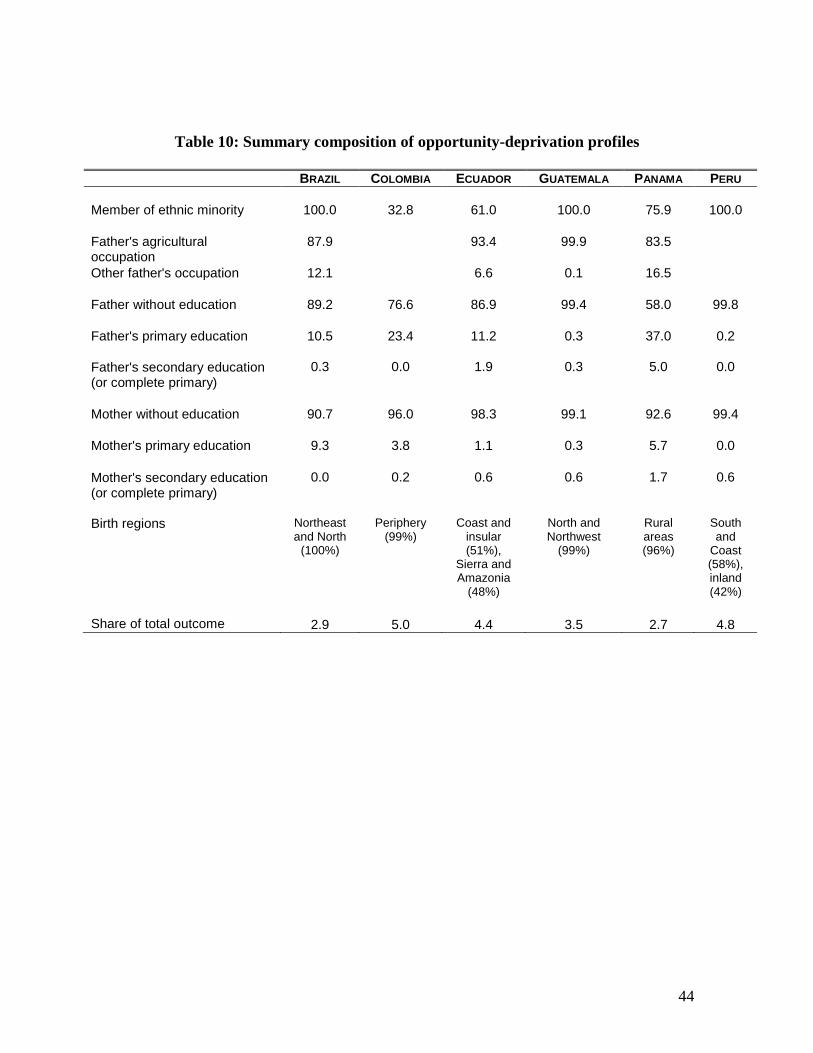
44

Table 10: Summary composition of opportunity-deprivation profiles

BRAZIL COLOMBIA ECUADOR GUATEMALA PANAMA PERU

Member of ethnic minority 100.0 32.8 61.0 100.0 75.9 100.0

Father's agricultural occupation

87.9 93.4 99.9 83.5

Other father's occupation 12.1 6.6 0.1 16.5

Father without education 89.2 76.6 86.9 99.4 58.0 99.8

Father's primary education 10.5 23.4 11.2 0.3 37.0 0.2

Father's secondary education (or complete primary)

0.3 0.0 1.9 0.3 5.0 0.0

Mother without education 90.7 96.0 98.3 99.1 92.6 99.4

Mother's primary education 9.3 3.8 1.1 0.3 5.7 0.0

Mother's secondary education (or complete primary)

0.0 0.2 0.6 0.6 1.7 0.6

Birth regions Northeast

and North (100%)

Periphery (99%)

Coast and insular (51%),

Sierra and Amazonia

(48%)

North and Northwest

(99%)

Rural areas (96%)

South and

Coast (58%), inland (42%)

Share of total outcome 2.9 5.0 4.4 3.5 2.7 4.8

45

Figure 1: The distribution of consumption conditional on selected circumstance

variables

a. By mother‟s education 0

.2.4

.6.8

1

-2 -1 0 1 2consumption

none incomplete

primary complete

Colombia

0.2

.4.6

.81

-2 -1 0 1 2consumption

none incomplete

primary complete

Ecuador

0.2

.4.6

.81

-2 -1 0 1 2consumption

none incomplete

primary complete

Guatemala

0.2

.4.6

.81

-2 -1 0 1 2consumption

none incomplete

primary complete

Panama

0.2

.4.6

.81

-2 -1 0 1 2consumption

none incomplete

primary complete

Peru

b. By ethnicity

0.2

.4.6

.81

-2 -1 0 1 2consumption

minority others

Colombia

0.2

.4.6

.81

-2 -1 0 1 2consumption

minority others

Ecuador

0.2

.4.6

.81

-2 -1 0 1 2consumption

minority others

Guatemala

0.2

.4.6

.81

-2 -1 0 1 2consumption

minority others

Panama

0.2

.4.6

.81

-2 -1 0 1 2consumption

minority others

Peru