arX

iv:1

507.

0519

1v1

[ast

ro-p

h.S

R]

18 J

ul 2

015

Astronomy & Astrophysicsmanuscript no. arxiv˙ZP c© ESO 2015July 21, 2015

The Maunder minimum (1645–1715) was indeed a Grandminimum: A reassessment of multiple datasets

Ilya G. Usoskin1,2, Rainer Arlt3, Eleanna Asvestari1, Ed Hawkins6, Maarit Kapyla7, Gennady A. Kovaltsov4, NatalieKrivova5, Michael Lockwood6, Kalevi Mursula1, Jezebel O’Reilly6, Matthew Owens6, Chris J. Scott6, Dmitry D.

Sokoloff8,9, Sami K. Solanki5,10, Willie Soon11, and Jose M. Vaquero12

1 ReSoLVE Centre of Excellence, University of Oulu, Finland2 Sodankyla Geophysical Observatory, University of Oulu, Finland3 Leibniz Institute for Astrophysics Potsdam, An der Sternwarte 16, 14482 Potsdam, Germany4 Ioffe Physical-Technical Institure, St. Petersburg, Russia5 Max Planck Institute for Solar System Research, Justus-von-Liebig-Weg 3, 37077 Gottingen, Germany6 Department of Meteorology, University of Reading, U.K.7 ReSoLVE Centre of Excellence, Department of Computer Science, PO BOX 15400, Aalto University FI-00076 Aalto, Finland8 Moscow State University, Moscow, Russia9 IZMIRAN, Moscow, Russia

10 School of Space Research, Kyung Hee University, Yongin, Gyeonggi 446-701, Republic of Korea11 Harvard-Smithsonian Center for Astrophysics, Cambridge,MA, USA12 Departamento de Fısica, Universidad de Extremadura, Merida (Badajoz), Spain

ABSTRACT

Aims. Although the time of the Maunder minimum (1645–1715) is widely known as a period of extremely low solar activity, claims are stilldebated that solar activity during that period might still have been moderate, even higher than the current solar cycle #24. We have revisited allthe existing pieces of evidence and datasets, both direct and indirect, to assess the level of solar activity during the Maunder minimum.Methods. We discuss the East Asian naked-eye sunspot observations, the telescopic solar observations, the fraction of sunspot active days, thelatitudinal extent of sunspot positions, auroral sightings at high latitudes, cosmogenic radionuclide data as well assolar eclipse observations forthat period. We also consider peculiar features of the Sun (very strong hemispheric asymmetry of sunspot location, unusual differential rotationand the lack of the K-corona) that imply a special mode of solar activity during the Maunder minimum.Results. The level of solar activity during the Maunder minimum is reassessed on the basis of all available data sets.Conclusions. We conclude that solar activity was indeed at an exceptionally low level during the Maunder minimum. Although the exact levelis still unclear, it was definitely below that during the Dalton minimum around 1800 and significantly below that of the current solar cycle # 24.Claims of a moderate-to-high level of solar activity duringthe Maunder minimum are rejected at a high confidence level.

Key words. Sun:activity - Sun:dynamo - Sun:Maunder Minimum

1. Introduction

In addition to the dominant 11-year Schwabe cycle, solar ac-tivity varies on the centennial time scale (Hathaway, 2010).It is a common present-day paradigm that the Maunder min-imum (MM), occurring during the interval 1645–1715 (Eddy,1976), was a period of greatly suppressed solar activity calleda Grand minimum. Grand minima are usually considered asperiods of greatly suppressed solar activity corresponding to aspecial state of the solar dynamo (Charbonneau, 2010). Of spe-cial interest is the so-called core MM (1645–1700) when cyclicsunspot activity was hardly visible (Vaquero & Trigo, 2015).While such Grand minima are known, from the indirect evi-dence provided by the cosmogenic isotopes14C and10Be data

for the Holocene, to occur sporadically, with the Sun spend-ing on average1/6 of the time in such a state (Usoskin et al.,2007), the MM is the only Grand minimum covered by di-rect solar (and some relevant terrestrial) observations. It there-fore forms a benchmark for other Grand minima. We notethat other periods of reduced activity during the last cen-turies, such as the Dalton minimum at the turn of the 18thand 19th centuries, the Gleissberg minimum around 1900, orthe weak present solar cycle #24, are also known but they aretypically not considered to be Grand minima (Schussler et al.,1997; Sokoloff, 2004). However, the exact level of solar ac-tivity in the 17th century remains somewhat uncertain (e.g.Vaquero & Vazquez, 2009; Vaquero et al., 2011; Clette et al.,2014), leaving room for discussions and speculations. For ex-

2 Usoskin et al.: Maunder minimum: A reassessment

ample, there have been several suggestions that sunspot activitywas moderate or even high during the core MM (1645–1700),being comparable to or even exceeding the current solar cy-cle #24 (Schove, 1955; Gleissberg et al., 1979; Cullen, 1980;Nagovitsyn, 1997; Ogurtsov et al., 2003; Nagovitsyn et al.,2004; Volobuev, 2004; Rek, 2013; Zolotova & Ponyavin,2015). Some of these were based on a mathematical synthe-sis using empirical rules in a way similar to Schove (1955)and Nagovitsyn (1997), and therefore are not true reconstruc-tions. Some others used a re-analysis of the direct data series(Rek, 2013; Zolotova & Ponyavin, 2015) and provide claimedassessments of the solar variability. While earlier suggestionshave been convincingly rebutted by Eddy (1983), the most re-cent ones are still circulating. If such claims were true, thenthe MM would not be a Grand minimum. This would poten-tially cast doubts upon the existence of any Grand minimum,including those reconstructed from cosmogenic isotopes.

There are indications that the underlying solar mag-netic cycles still operated during the MM (Beer et al., 1998;Usoskin et al., 2001), but at the threshold level as proposedal-ready by Maunder (1922):

It ought not to be overlooked that, prolonged as this in-activity of the Sun certainly was, yet few stray spotsnoted during “the seventy years’ death”– 1660, 1671,1684, 1695, 1707, 1718 [we are, however, less certainabout the exact timings of these activity maxima]– cor-respond, as nearly as we can expect, to the theoreticaldates of maximum. ... If I may repeat the simile whichI used in my paper forKnowledge in 1894, “just as ina deeply inundated country, the loftiest objects will stillraise their heads above the flood, and a spire here, a hill,a tower, a tree there, enable one to trace out the con-figuration of the submerged champaign,” to the abovementioned years seem be marked out as the crests of asunken spot-curve.

The nature of the MM is of much more than purelyacademic interest. A recent analysis of cosmogenic isotopedata revealed a 10% chance that Maunder minimum condi-tions would return within 50 years of now (Lockwood, 2010;Solanki & Krivova, 2011; Barnard et al., 2011). It thereforebe-comes of practical importance to accurately describe and un-derstand the MM, since a future Grand minimum is expectedto have significant implications for space climate and spaceweather.

Here we present a compilation of observational and his-torical facts and evidence showing that the MM was indeed aGrand minimum of solar activity and that the level of solar ac-tivity was very low, much lower than that during the Daltonminimum as well as the present cycle # 24 . In Section 2 we re-visit sunspot observations during the MM. In Section 3 we an-alyze indirect proxy records of solar activity, specifically auro-rae borealis and cosmogenic isotopes. In Section 4 we discussconsequences of the MM for solar dynamo and solar irradiancemodelling. Conclusions are presented in Section 5.

1650 1700

0

50

100

GS

N

Years

GSN

V15 (strict)

V15 (loose)

ZP15

Fig. 1. Annual group sunspot numbers during and around theMaunder minimum, according to Hoyt & Schatten (1998) -GSN, Zolotova & Ponyavin (2015) – ZP15, and loose andstrictly conservative models from Vaquero et al. (2015a) (seeSect. 2.1), as denoted in the legend.

2. Sunspot observation in the 17th century

Figure 1 shows different estimates of sunspot activity, quan-tified in terms of the annual group sunspot number (GSN)RG, around the MM. The conventional GSN (Hoyt & Schatten,1998, called HS98 henceforth), with the recent corrections, re-lated to newly uncovered data or corrections of earlier errors,applied (see details in Vaquero et al., 2011; Vaquero & Trigo,2014; Lockwood et al., 2014b), is shown as the black curve.This series, however, contains a large number of generic no-spot statements (i.e. statements that no spots were seen on theSun during long periods), which should be treated with cau-tion (Kovaltsov et al., 2004; Vaquero, 2007; Clette et al., 2014;Zolotova & Ponyavin, 2015; Vaquero et al., 2015a, see alsoSect. 2.3). Figure 1 shows also two recent estimates of the an-nual GSN by Vaquero et al. (2015a), who treated generic no-sunspot records in the HS98 catalog in a conservative way. Thesunspot numbers were estimated using the active-vs-inactiveday statistics (see Sect. 2.1, full details in Vaquero et al.,2015a). All these results lie close to each other and implyvery low sunspot activity during the MM. On the contrary,Zolotova & Ponyavin (2015), called henceforth ZP15, arguefor higher sunspot activity in the MM (the red dotted curvein Figure 1 is taken from Figure 13 of ZP15), with the sunspotcycles being not smaller than a GSN of 30 and even reaching90–100 during the core MM.

For subsequent analysis we consider two scenarios of so-lar activity, reflecting the opposing views on the level ofsolar activity around the MM before 1749: (1) L-scenarioof low activity during the MM, as based on the conven-tional GSN (Hoyt & Schatten, 1998) with the recent correc-tions implemented (see Lockwood et al., 2014b, for details)– see black curve in Fig. 1; (2) H-scenario of high activ-ity during the MM, based on GSN as proposed by ZP15(red dotted curve in Fig. 1). This scenario qualitatively repre-sents also other suggestions of high activity (e.g., Nagovitsyn,1997; Ogurtsov et al., 2003; Volobuev, 2004). After 1749,both scenarios are extended by the International sunspot num-ber (http://sidc.oma.be/silso/datafiles). We use annual values

Usoskin et al.: Maunder minimum: A reassessment 3

throughout the paper unless another time resolution is explic-itly mentioned.

2.1. Fraction of active days

High solar cycles imply that≈ 100% of days are active,and sunspots are seen on the Sun almost every day dur-ing such cycles, except for a few years around cycle min-ima (Kovaltsov et al., 2004; Vaquero et al., 2012, 2014). If thesunspot activity was high during the MM, as proposed by theH-scenario, the Sun must have been displaying sunspots almostevery day. However, this clearly contradicts with the data,sincethe reported sunspot days, also those reported by active ob-servers, cover only a small fraction of the year even around theproposed cycle maxima (see Fig. 2 in Vaquero et al., 2015a).Thus, either one has to assume a severe selection bias for ob-servers reporting only a few sunspot days per year while spotswere present all the time, or to accept that indeed spots wererare.

During periods of weak solar activity, the fraction ofspotless days is a very sensitive indicator of the ac-tivity level (Harvey & White, 1999; Kovaltsov et al., 2004;Vaquero & Trigo, 2014), much more precise than the sunspotcounts. However, this quantity tends to zero (almost all daysare active) when the average sunspot number exceeds 20(Vaquero et al., 2015a). Vaquero et al. (2015a) considered sev-eral statistically conservative models to assess the sunspotnumber during the MM from the active day fraction. The”loose” model ignores all generic no-spot statements and ac-cepts only explicit no-spot records with exact date and ex-plicit statements of no spots on the Sun, while the ”strict”model considers only such explicit statements as in the ”loose”model but made by at least two independent observers for thespotless days. In this way, the possibility of omitting spots isgreatly reduced since the two observers would have to omit thesame spot independently. The strict model can be consideredas the most generous upper bound to sunspot activity duringthe MM. However, it most likely exaggerates the activity byover-suppressing records reporting no spots on the Sun. Thesemodels are shown in Fig. 1 One can see that these estimatesyield sunspot numbers that do not exceed 5 (15) for the ”loose”(”strict”) model during the MM.

2.2. Occidental telescopic sunspot observations:Historical perspective

The use of the telescope for astronomical observations be-came widespread quickly after 1609. We know that there weretelescopes with sufficient quality and size to see even smallspots, in the second half of the 17th century. It is also knownthat astronomers of that era used other devices in their rou-tine observations such as mural quadrants or meridian lines(Heilborn, 1999). However, as proposed by ZP15, the qualityof the sunspot data for that period might be compromised bynon-scientific biases.

2.2.1. Dominant world view

Recently, ZP15 suggested that scientists of the 17th centurymight be influenced by the “dominant worldview of the sev-enteenth century that spots (Sun’s planets) are shadows froma transit of unknown celestial bodies”, and that “an object onthe solar surface with an irregular shape or consisting of a setof small spots could have been omitted in a textual report be-cause it was impossible to recognize that this object is a celes-tial body”. This would suggest that professional astronomers ofthe 17th century, even if technically capable of observing spots,might distort the actual records for politically/religiously mo-tivated, non-scientific reasons. This was the key argument forZP15 to propose the high solar activity during the MM. Belowwe discuss that, on the contrary, scientists of the 17th centurywere reporting sunspots quite objectively.

Sunspots: Planets or solar features?There was a controversy in the first decades of the 17th centuryabout location of sunspots: either on the Sun (like clouds),ororbiting at a distance (as a planet). However, already Scheinerand Hevelius plotted non-circular plots and showed the per-spective foreshortening of spots near the limb. In his AccuratiorDisquisito, Christoph Scheiner (1612) wrote pseudonymouslyas ‘Appelles waiting behind the picture’ and detailed the ap-pearance of spots as of irregular shape and variable, and finallyconcluded (Galileo & Scheiner, 2010):

They are not to be admitted among the number of stars,because they are of an irregular shape, because theychange their shape, because they [. . . ] should alreadyhave returned several times, contrary to what has hap-pened, because spots frequently arise in the middle ofthe Sun that at ingress escaped sharp eyes, becausesometimes some disappear before having finished theircourse.

Even though Scheiner had believed until this point thatsunspots were bodies or other entities just outside the Sun,hedid note all their properties very objectively. Later, Scheiner(1630) concluded in his comprehensive book on sunspots,“Maculæ non sunt extra solem” (spots are not outside theSun, p. 455ff.) and even “Nuclei Macularum sunt profundi”(the cores of sunspots are deep, p. 506). On the contrary,Smogulecz & Schonberger (1626) who were colleagues ofScheiner in Ingolstadt and Freiburg-im-Breisgau, respectively,called the spots “stellaæ solares” (= solar stars) which wasmeant in the sense of moons. Some authors, especially anti-Copernican astronomers, such as Antonius Maria Schyrleusof Rheita (1604–1660) (see Gomez & Vaquero, 2015) andCharles Malapert (1581–1630), followed the planetary model.On the other hand, Galileo had geometrically demonstrated(using the measured apparent velocities of crossing the solardisc) that spots are located on the solar surface. In fact, thechanges in the trajectory of sunspots on the ”solar surface”were an important element of discussion in the context of he-liocentrism (Smith, 1985; Hutchison, 1990; Topper, 1999).

It was clear already in that time that sunspots are not plan-ets, for reasons of the form, color, shape of the spots nearthe limb and their occasional disappearance in the middle of

4 Usoskin et al.: Maunder minimum: A reassessment

the disk. A nice example of the kind is given in a letter toWilliam Gascoigne (1612–1644), that William Crabtree wroteon 7 August 1640 (= Aug 17 greg.) (Chapman, 2004), as pub-lished by Derham & Crabtrie (1711):

I have often observed these Spots; yet from all myObservations cannot find one Argument to prove themother than fading Bodies. But that they are no Stars, butunconstant (in regard of their Generation) and irregu-lar Excrescences arising out of, or proceeding from theSun’s Body, many things seem to me to make it morethan probable.

Although some astronomers still believed in the mid-17thcentury that sunspots were small planets orbiting the Sun,the common paradigm among the astronomers of that timewas “that spots were current material features on the verysurface of the Sun” (Brody, 2002, page 78). Therefore, ob-servers of sunspots during the MM, in particular professionalastronomers, did not adhere to the ”dominant worldview” ofthe planetary nature of sunspots and hence were not stronglyinfluenced by it, contrary to the claim of ZP15.

Galileo’s trial.We note that the problem in the trial of Galileo was not theCopernican system, but the claim that astronomical hypothe-ses can be validated or invalidated (an absurd presumption formany people of the early 17th century) and the potential claimof re-interpreting the Bible (Schroder, 2002). The planetarysystem was considered as a mathematical tool to compute themotion of the planets as precisely as possible; it was not a sub-ject to be proven. This subtle difference was an important issuein the first half of the 17th century to comply with the require-ments of the catholic church. While an entire discussion of thevarious misconceptions about the Galileo trial is beyond thescope of this Paper, there are many indications that the natureand origin of celestial phenomena had been discussed by thescholars of the 17th century, rather than discounted by a stan-dard world view. We are not aware of any documental evidencethat writing about sunspots was prohibited or generally dislikedby the majority of observers in any document.

Shape of sunspots.ZP15 presented a hand-picked selection of a few drawings tosupport their statement that “there was a tendency to drawsunspots as objects of a circularized form”, but there are plentyof other drawings from the same time showing sunspots ofirregular shape and sunspot groups with complex structures.Here we show only a few of numerous examples. Figure 2depicts a sunspot group observed in several observatories inEurope in August 1671. A dominant spot with a complex struc-ture having multiple umbrae within the same penumbra and agroup of small spots in its surroundings can be appreciated.Another example (Figure 3) shows a spot drawing by G.D.Cassini in 1671 (Oldenburg, 1671c)1, which illustrates thecomplexity and non-circularity as well as the foreshortening

1 Henry Oldenburg was Secretary of the Royal Society and com-piled findings from letters of other scientists in the PhilosophicalTransactions in his own words. We therefore cite his name although itis not given for the actual article.

Fig. 2. Drawing of a sunspot group observed in August 1671,as published in number 75 of the Philosophical Transactions,corresponding to August 14, 1671.

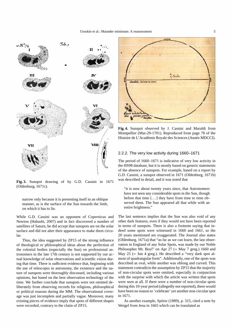
of sunspots very clearly. Finally, Figure 4 displays a sunspotobservation made by J. Cassini and Maraldi from Montpellier(Mar-29-1701). There is a small sunspot group (labelled as A)approximately in the middle of the solar disc which is zoomedin the bottom left corner, exhibiting a complex structure, and alegend that reads “Shape of the Spot observed with a large tele-scope”. These drawings are not limited to “circularized forms”,and such instances are numerous.

It is important that observers who made drawings actuallyretained the perspective foreshortening of the spots near thesolar limb. Galilei (1613), Scheiner (1630), Hevelius (1647),G.D. Cassini in 1671 (Oldenburg, 1671c) as well as Cassini(1730, observation of 1684), P. De La Hire (1720, observationof 1703), and Derham (1703) all drew slim, non-circular spotsnear the edge of the Sun. It was clear to them that those ob-jects cannot be spheres. They were not shadows either sincethat would require an additional light source similar to theSunwhich is not observed. A note by G.D. Cassini of 1684 says(Cassini, 1730):

This penumbra is getting rounder when the spot ap-proaches the center, as it is always happening, this isan indication that this penumbra is flat, and that it looks

Usoskin et al.: Maunder minimum: A reassessment 5

Fig. 3. Sunspot drawing of by G.D. Cassini in 1671(Oldenburg, 1671c).

narrow only because it is presenting itself in an obliquemanner, as is the surface of the Sun towards the limb,on which it has to lie.

While G.D. Cassini was an opponent of Copernicus andNewton (Habashi, 2007) and in fact discovered a number ofsatellites of Saturn, he did accept that sunspots are on the solarsurface and did not alter their appearance to make them circu-lar.

Thus, the idea suggested by ZP15 of the strong influenceof theological or philosophical ideas about the perfectionofthe celestial bodies (especially the Sun) on professional as-tronomers in the late 17th century is not supported by our ac-tual knowledge of solar observations and scientific vision dur-ing that time. There is sufficient evidence that, beginning withthe use of telescopes in astronomy, the existence and the na-ture of sunspots were thoroughly discussed, including variousopinions, but based on the best observation technology of thetime. We further conclude that sunspots were not omitted de-liberately from observing records for religious, philosophicalor political reasons during the MM. The observational cover-age was just incomplete and partially vague. Moreover, manyexisting pieces of evidence imply that spots of different shapeswere recorded, contrary to the claim of ZP15.

Fig. 4. Sunspot observed by J. Cassini and Maraldi fromMontpellier (Mar-29-1701). Reproduced from page 78 of theHistoire de L’Academie Royale des Sciences (Annee MDCCI).

2.2.2. The very low activity during 1660–1671

The period of 1660–1671 is indicative of very low activity inthe HS98 database, but it is mostly based on generic statementsof the absence of sunspots. For example, based on a report byG.D. Cassini, a sunspot observed in 1671 (Oldenburg, 1671b)was described in detail, and it was noted that

“it is now about twenty years since, that Astronomershave not seen any considerable spots in the Sun, thoughbefore that time [. . . ] they have from time to time ob-served them. The Sun appeared all that while with anentire brightness.”

The last sentence implies that the Sun was also void of anyother dark features, even if they would not have been reportedin terms of sunspots. There is also a footnote saying that in-deed some spots were witnessed in 1660 and 1661, so the20 years mentioned are exaggerated. The Journal also states(Oldenburg, 1671a) that “as far as we can learn, the last obser-vation in England of any Solar Spots, was made by our NoblePhilosopher Mr. Boyl” on Apr 27 (= May 7 greg.) 1660 andMay 25 (= Jun 4 greg.). He described a “very dark spot al-most of quadrangular form”. Additionally, one of the spots wasdescribed as oval, while another was oblong and curved. Thisstatement contradicts the assumption by ZP15 that the majorityof non-circular spots were omitted, especially in conjunctionwith the surprise with which the article was written that spotswere seen at all. If there were a number of non-circular spotsduring this 10-year period (allegedly not reported), therewouldhave been no reason to ‘celebrate’ yet another non-circularspotin 1671.

As another example, Sporer (1889), p. 315, cited a note byWeigel from Jena in 1665 which can be translated as

6 Usoskin et al.: Maunder minimum: A reassessment

Many diligent observers of the skies have wonderedhere that for such a long time no spots were notice-able on the Sun. And we need to admit here in Jenathat, despite having tried in many ways, setting up largeand small spotting scopes pointed to the Sun, we havenot found such phenomena for a considerable amountof time.

Since the notes on the absence of spots come from variouscountries and from catholic, protestant and Anglican people,we believe there was no wide-spread religious attitude to with-hold spots in order to save the purity of the Sun.

The only positive sunspot report between 1660 and 1671in the HS98 database is the one by Kircher in 1667. This datapoint comes from a note (Frick, 1681, p. 49) stating that

the late Christoff Weickman, who was experienced inoptics and made a number of excellent telescopes,watched the Sun at various times hoping to see the like[sunspots] on the Sun, but could never get a glimpse ofthem [. . . ] So Mr Weickman wrote to Father Kircherand uncovered him that he could not see such things onthe Sun, does not know why this is or where the mis-take could be. Father Kircher answered from Rome on2 September 1667 that it happens very rarely that onecould see the Sun as such; he had not seen it in such amanner more than once, namely Anno 1636.

One can see that the date of the letter in 1667 was mistakenlyconsidered as the observing date. Instead the report clearly in-dicates that no sunspots were seen at all by Weickman in the1660s. The sunspot observation by Kircher in 1667 is erro-neous and needs to be removed from the HS98 database. Thenno indication of sunspots exists in the 1660s. We note that thisfalse report was used by ZP15 to evaluate the sunspot cyclemaximum around that date.

2.3. Generic statements and gaps in the HS98database

The database of HS98 forms a basis to many studies of sunspotsrecords during the period under investigation. In particular,ZP15 based their arguments on this database without referringto the original records. However, it contains a number of notobvious features which can be easily misinterpreted if not con-sidered properly. Here we discuss such features which are di-rectly related to the evaluation of sunspot activity in the 17thcentury.

In particular, many no-spot records were related to astro-metric observations of the Sun such as solar meridian altitudeor the apparent solar diameter (Vaquero & Gallego, 2014). Forexample, Manfredi (1736) listed more than 4200 solar merid-ian observations made by several scientists during 1655-1736using the gigantic camera obscura installed on the floor of theBasilica of San Petronio in Bologna. Such observations werenot focused on sunspots and did not include any mentioningof spots. However, HS98 treated all these reports as observa-tions of the absence of sunspot groups which, of course, wasincorrect.

HS98 database contains gaps of the observing records ofMarius and Riccioli, that occur exactly during days when otherobservers reported spots, which was interpreted by ZP15 asindications that they deliberately stopped reporting to hidesunspots: “It is noteworthy that when the Sun became active,Marius and Riccioli immediately stopped observations.”. Wenote that this interpretation is erroneous and based on igno-rance of the detail of the HS98 database as explained below.

The original statement by Marius from Apr 16 (= Apr 26greg.) 1619, on which this series is based, is

While I did not find as many spots in the disk of theSun over the past one-and-a-half years, often not even asingle spot, which was never seen in the year before, Inoted in my observing diary: Mirum mihi videtur, adeoraras vel sæpius nullas maculas in disco solis depre-hendi, quod ante hac nunque est observatum

which is a Latin repetition of what he said before. Mariusclearly states that the sunspot number was not exactly zero,butvery low. HS98 have used this statement to approximate theactivity by zeros in their database, more precisely by filling alldates of the 1.5-yr interval with zeros except the periods whenother observers did see spots. The existence of the gaps is byno means based on the actual observing report by Marius, butis an effect of the way HS98 have interpreted the comment.

The same reason holds for the gaps in the sunspots re-ported by Riccioli (1653), p. 96, whose data (zeros) in the HS98database are based on the statement that

. . . in the year 1618 when a comet and tail shone,no spots were observed, said Argolus in PandosionSphæricum chapter 44.

The original statement by Argolus (1644), p. 213, states: “Anno1618 tempore quo Trabs, et Cometa affulsit nulla visa est.”Apart from the fact that it was not Riccioli himself who ob-served, this again led to filling all days in 1618 with zeros (inthe HS98 database) except the days when other observers sawspots.

The method of filling the HS98 database for many monthsand even years with zeros is based on generic verbal reports onthe absence of spots for long periods also in the cases of Picard,G.D. Cassini, Dechales, Maraldi, Siverus and others (see, e.g,Vaquero et al., 2011; Vaquero et al., 2015a). HS98 must havefilled those periods in the sense of probably very low activ-ity, but they are not meant to provide exact timings of obser-vations, as ZP15 interpreted them. The appearance of gaps inzero records when other observers reported spots is not an in-dication of withholding spots in observing reports but rather asimple technical way of avoiding conflicting data in the HS98database. ZP15 mistook the entries in the HS98 database foractual observing dates and interpreted them incorrectly.

While assuming a large number of days without spots isa significant underestimation of the solar activity on the onehand, as shown by Vaquero et al. (2015a) and has been pointedout by ZP15 as well, the assumption that observers deliberatelystopped reporting is, on the other hand, not supported by anyoriginal text and remains an ungrounded speculation.

Usoskin et al.: Maunder minimum: A reassessment 7

The observations by Hevelius of 1653–1684 as recoveredby Hoyt & Schatten (1995) should also be scrutinized with re-gard to a possible omission of spots. Citing the former refer-ence, ZP15 even claim that “Hevelius quite consciously didnot record sunspots”, while the original statement was that“Hevelius occasionally missed sunspots but usually was a re-liable observer.” Actually, out of 24 groups that could havebeen detected by Hevelius given his observing days, he saw20 (Hoyt & Schatten, 1995). He never reported the absence ofsunspots when others saw them. The four occasions are simplynot accompanied by any statement about presence or absenceof spots. This can be understood considering that the sunspotnotes are just remarks on his solar elevation measurements(Hevelius, 1679, part 3). Those, however, were made with aquadrans azimutalis which had no telescope, since Heveliusre-fused to switch to a telescope at some point, perhaps becausehedid not want to spoil his time series of measurements (Habashi,2007). He therefore could not see sunspots at all with his de-vice and had to take an additional instrument to observe them,and it is probable that he did not do so on each day he mea-sured the solar elevation, hence left so many days neither withpositive nor with negative information on sunspots. We havetotreat those as non-observations.

2.4. Methodological errors of ZP15

The original work by ZP15 unfortunately contains a number ofmethodological errors which eventually led them to an extremeconclusion that sunspot activity during the MM was at a mod-erate to high level. In particular, ZP15 sometimes incorrectlyinterpreted published records. Moreover they used the originaluncorrected record of HS98, while numerous corrections havebeen made to that during the last 17 years (e.g. Vaquero et al.,2011; Vaquero & Trigo, 2014; Carrasco et al., 2015). Here wediscuss some of the errors in ZP15, as examples of erroneousinterpretation of historical data, in detail.

2.4.1. Sunspot drawings vs. textual notes

According to ZP15 “sunspot drawings provide a significantlylarger number of sunspots, compared to textual or tabularsources”. This is trivial considering that the tabular sourcesoften are related to astrometric observations of the Sun suchas solar meridian altitude or the apparent solar diameter(Vaquero & Gallego, 2014). However, if one considers onlythose tabular sources that contain explicit information about thepresence or absence of sunspots then drawing sources appeartobe consistent with the reliable tabular sources (Kovaltsovet al.,2004; Carrasco et al., 2015).

The main assumption in ZP15 is that sunspots were omit-ted, especially in verbal reports, if they were not round anddidnot resemble a planet. The only direct example of that is given,with a reference to Vaquero & Vazquez (2009), that Harriotdrew three sunspots on Dec 8 (= Dec 18 greg.) 1610 but wrotethat the Sun was “clear”. However, this discussion was basedon an incorrect interpretation of the original texts. The actualstatement of Harriot (1613) is

The altitude of the sonne being 7 or 8 degrees. It beinga frost and a mist. I saw the sonne in this manner [draw-ing]. I saw it twise or thrise. Once with the right ey andother time with the left. In the space of a minute time,after the sonne was to cleare.

As indicated by the observing times and numerous other state-ments about a “well tempered” Sun in the course of his ob-servations, he mostly observed near sunrise or sunset or with acertain cloud cover to be able to look through the telescope.Thestatement that “the sonne was to cleare” refers to the fact thatthe Sun became too bright after a few minutes of observing. Inthis context, “cleare” means “bright” and not clear or spotless.Therefore, this example was incorrectly taken by ZP15 as an il-lustrative case of the discrepancy between textual and drawingsources.

As another example, we compared the textual recordsby Smogulecz & Schonberger (1626), who had conservativeviews on sunspots (see Sect. 2.2.1), with the drawings made byScheiner in Rome for the same period of 1625. We found thatthat Smogulecz and Schonberger omitted a number of spotsfrom the drawings, but mentioned all spots they saw in their text(calling them ‘stellæ’), in accordance with Scheiner. Thisis incontradiction with the assumption of ZP15 that verbal reportsare subject to withholding spots. Table 1 lists the numbers ofspots mentioned in their text versus those drawn in the figures.(We note that the values are also incorrectly used in HS98.)Smogulecz & Schonberger (1626) selected certain spots whichwere visible long enough to measure the obliquity of the Sun’saxis with the ecliptic and plotted them schematically as circlesas not particularly interested in their shape.

2.4.2. Relation between maximum number of sunspotgroups and sunspot number

ZP15 proposed a new method to assess the amplitude of the so-lar cycle during the MM. As the amplitude of a sunspot cycle,A∗G, they used themaximum daily number of sunspot groupsG∗ during the cycle, so thatA∗G = 12.08×G∗, where the coeffi-cient 12.08 is a scaling between the average number of sunspotgroups and the sunspot number (Hoyt & Schatten, 1998). Wenote that using the maximum daily value ofG∗ instead of theaverage valueG leads to a large overestimate of the sunspotcycle amplitude, particularly during the MM. We analyze theHS98 database for the period 1886–1945, when sunspot cycleswere not very high, to compare the annually averaged groupsunspot numbersRG and the annual values ofA∗G obtained us-ing the annual maxima of the daily sunspot group numbersG∗.Fig. 5a shows a scatter plot of the annual values ofRG andG∗ (dots), while the dashed line gives an estimate of theA∗Gbased onG∗, following the recipe of ZP15. One can see thatwhile there is a relation between annualRG andG∗, the pro-posed method heavily overestimates the annual sunspot activ-ity. Fig. 5b shows the overestimate factorY = A∗G/RG of thesunspot numbers as a function ofG∗. While the factorY is 2–3for very active years withG∗ > 15, the overestimate can reachan order of magnitude for years with weaker activity, such asduring the MM. When applying to the sunspot cycle amplitude,

8 Usoskin et al.: Maunder minimum: A reassessment

Table 1. Comparison of the number of spots listed in the ver-bal reports versus the number of spots in the drawings bySmogulecz & Schonberger (1626) in 1625.

Date Text Drawn Date Text Drawn1625 Jan 14 1 1 1625 Aug 22 2 11625 Jan 15 1 1 1625 Aug 23 2 11625 Jan 16 4 1 1625 Aug 27 6 11625 Jan 17 8 1 1625 Aug 28 10 11625 Jan 18 2 1 1625 Aug 31 7 11625 Jan 19 4 1 1625 Sep 01 6 11625 Jan 20 2 1 1625 Sep 05 8 41625 Feb 12 8 1 1625 Sep 07 6 31625 Feb 16 10 1 1625 Sep 08 6 31625 Feb 17 11 1 1625 Sep 11 5 31625 Feb 18 10 1 1625 Sep 12 4 31625 Feb 21 4 1 1625 Sep 13 2 21625 Jun 01 9 1 1625 Oct 05 9 81625 Jun 04 3 1 1625 Oct 06 2 11625 Jun 05 3 1 1625 Oct 09 4 41625 Jun 06 2 1 1625 Oct 10 7 81625 Jun 07 3 1 1625 Oct 11 9 91625 Jun 09 2 1 1625 Oct 13 2 11625 Aug 08 6 1 1625 Oct 14 2 11625 Aug 09 4 1 1625 Oct 15 3 11625 Aug 10 2 1 1625 Oct 25 1 11625 Aug 12 4 2 1625 Oct 26 1 11625 Aug 13 3 2 1625 Oct 27 1 11625 Aug 14 3 2 1625 Oct 28 1 11626 Aug 15 4 2 1625 Oct 29 1 11625 Aug 17 2 2 1625 Oct 31 1 11625 Aug 18 4 2 1625 Nov 01 1 11625 Aug 19 2 1

the error becomes even more severe. Thus, by taking the cyclemaxima of the daily number of sunspot groups instead of theirannual means, ZP15 systematically overestimated the sunspotnumbers during the MM by a factor of 5–15.

The number of sunspot groups in 1642.ZP15 proposed that the solar cycle just before the MM washigh (sunspot number≈ 100) which is based on a report of8 sunspot groups observed by Antonius Maria Schyrleus ofRheita in February 1642 as presented in the HS98 database.However, as shown by Gomez & Vaquero (2015), this recordis erroneous in the HS98 database because it is based on an in-correct translation from the original Latin records, whichsaysthat one (or a few) group was observed for 8 days in June 1642instead of 8 groups in February 1642. Accordingly, the max-imum daily number of sunspot groups reported for that cycleG∗ was 5, not 8, reducing the cycle amplitude claimed by ZP15(see Sect. 2.4.2) by about 40%.

The number of sunspot groups in 1652.The original HS98 record contains 5 sunspot groups for theday of Apr-01-1652, referring to observations by JohannesHevelius. Accordingly, this value (the highest dailyG∗ for thedecade) was adopted by ZP15 leading to the high proposedsunspot cycle during the 1650s. However, as discussed byVaquero & Trigo (2014) in great detail, this value of 5 sunspotgroups is an erroneous interpretation, by HS98 with reference

0

50

100

150

200

0 5 10 15 20 25 30

0

5

10

15

RG

A)

Facto

r Y

Maximum number of groups G*

B)

Fig. 5. Illustration of the incorrectness of the method used byZP15 to assess the group sunspot numberRG during the MM.Panel (A): Annual values ofRG as a function of the maximumdaily number of sunspot groupsG∗ for the same year in theHS98 catalogue for the period of 1886–1945; the dashed lineis the dependence ofA∗G = 12.08× G∗ used by ZP15. Panel(B): The overestimate factorY of the GSN by the ZP15 methodY = A∗G/RG.

to Wolf (1856), of the original Latin text by Hevelius say-ing that there were 5 spots in two distinct groups on the Sun.Accordingly, the correct value ofG∗ for that day should be 2not 5.

The number of sunspot groups in 1705.A high sunspot number of above 70 was proposed by ZP15for the year 1705 based on six sunspot groups reported by J.Plantade from Montpellier (the correction factor for this ob-server is 1.107 according to HS98) for the day Feb-13-1705.This observer was quite active with regular observations dur-ing that period, with 44 known daily observational reports forthe year 1705. For example, J. Plantade reported 2, 3, 6, and1 groups, respectively, for the days of Feb-11 through Feb-14.His reports also mention the explicit absence of spots from theSun after the group he had followed passed beyond the limb.However, he did not make any reports during long spotless peri-ods, and wrote notes again when a new sunspot group appeared.The average number of sunspot groups per day reported by J.Plantade for 1705 was 1.22, which is a factor of 5 lower thanthat adopted by ZP15 who only took the largest daily value (seeSect. 2.4.2). If one calculates the group sunspot number fromthe dataset of J. Plantade records for 1705 in the classical way,one obtains a value ofRG = 16.3 (1.22× 12.08× 1.107).

2.5. Butterfly diagram

According to sunspot drawings during some periods ofthe MM, a hint of the butterfly diagram has been iden-tified, particularly towards the end of the MM after1670 (Ribes & Nesme-Ribes, 1993; Soon & Yaskell, 2003;Casas et al., 2006). However, the latitudinal extent of the but-terfly wings was quite narrow, being within 15 for the coreMM (1645–1700) and 20 for the period around 1705, whilecycles before and after the MM had a latitudinal extent of 30

Usoskin et al.: Maunder minimum: A reassessment 9

or greater. This suggests that the sunspot occurrence during theMM was limited to a more narrow band than outside the MM.Here we compare the statistics of the latitudinal extend of thebutterfly diagram wings for solar cycles # 0 through 22 (cy-cles 5 and 6 are missing). The cycles #0 through 4 were cov-ered by digitized drawings made by Staudacher for the period1749–1792 (Arlt, 2008), cycles #7 through 10 (1825–1867)were covered by digitized drawings made by Samuel HeinrichSchwabe (Arlt et al., 2013), cycle # 8 by drawings of GustavSporer (Diercke et al., 2015), while the period after 1874 wasstudied using the Royal Greenwich Observatory (RGO) cat-alogue. Moreover, a machine-readable version of the sunspotcatalogues of the 19th century complied by Carrington, Petersand de la Rue has been released recently (Casas & Vaquero,2014). For each solar cycle we defined the maximum latitude(in absolute values without differentiating north and south)of sunspot occurrence. Since the telescopic instruments werepoorer during the MM than nowadays, for consistency we con-sidered only large spots with the projected spot area greaterthan 100 msd (millionths of the solar disc). The result is shownin Fig. 6 as a function of the cycle maximum (inRG). One cansee that there is a weak dependence for stronger cycles gen-erally having a larger latitudinal span (cf, e.g. Vitinsky et al.,1986; Solanki et al., 2008; Jiang et al., 2011b), but the latitu-dinal extent of the butterfly wing was always greater than 28

for the last 250 years. A robust link between the mean/rangelatitude of sunspot occurrence and cycle strength is related tothe dynamo wave in the solar convection zone and has beenempirically studied, e.g., by Solanki et al. (2008) or Jianget al.(2011a). Since the maximum latitudinal extent of sunspots dur-ing the MM was 15 (during the core MM) or 20 (around ca.1705), it suggests a weak toroidal field causing a narrower lat-itudinal range of sunspot formation during the MM. This con-clusion is in agreement with the results of a more sophisticatedanalysis by Ivanov & Miletsky (2011) who found that the lat-itudinal span of the butterfly diagram during the late part ofthe MM should be 15–20, i.e., significantly lower than duringthe normal cycles. One may assume that all the higher latitudespots were deliberately omitted by all the observers duringtheMM but we are not aware of such a bias.

We note that two data sets of sunspot latitudes during theMM have been recently recovered and translated into machine-readable format (Vaquero et al., 2015b). Using these data sets,a decadal hemispheric asymmetry index has been calculatedconfirming a very strong hemispherical asymmetry (sunspotsappeared mostly in the southern hemisphere) in the MM, as re-ported in earlier works (Sporer, 1889; Ribes & Nesme-Ribes,1993; Sokoloff & Nesme-Ribes, 1994). Another moderatelyasymmetric pattern was observed only in the beginning of theDalton minimum (Arlt, 2009; Usoskin et al., 2009b). Thus, thisindicates that the MM was also a special period with respect tothe distribution of sunspot latitudes.

2.6. East-Asian naked-eye sunspot observations

East-Asian chronicles reporting observations for about twomillennia, by unaided naked eyes, of phenomena that may

0 50 100 150 2000

15

30

45

La

titu

din

al sp

an

(d

eg

)

Cycle maximum

Fig. 6. Maximum latitudinal span of the butterfly diagram asa function of the cycle amplitude in annualRG for solar cy-cles # 0–4 and 7–22, accounting only for large spots (with areagreater than 100 msd). The dashed and dotted lines depict themaximum latitudinal extent of sunspot occurrence during thecore (1645–1700) and the entire MM (1645–1712).

be interpreted as sunspots have sometimes been used asan argument suggesting high solar activity during the MM(Schove, 1983; Nagovitsyn, 2001; Ogurtsov et al., 2003;Zolotova & Ponyavin, 2015). Such statements are based onan assumption that sunspots must be large to be observedand that this is possible only at a high level of solar activity.However, as shown below, this is not correct. While such his-torical records can be useful in a long-term perspective showingqualitatively the presence of several Grand minima during thelast two millennia (Clark & Stephenson, 1978; Vaquero et al.,2002; Vaquero & Vazquez, 2009) including also the MM, thisdataset is not useful for establishing the quantitative level of so-lar activity over short timespans due to the small number of in-dividual observations and/or the specific meteorological, soci-ological and historical conditions required for such record (seeChapter 2 in Vaquero & Vazquez, 2009). Moreover, it is veryimportant to indicate that the quality of the historical recordof naked-eye sunspot (NES) observations was not uniformthrough the ages (i.e. during the approximately two millienniacovered by the record). In fact, the quality of such records forthe last four centuries was much poorer than that for the 12th-15th centuries, due to a change in the type of historical sources.In particular, the data coverage was reduced greatly after 1600(see Figure 2.18 in Vaquero & Vazquez, 2009). There are veryfew NES records during the century between the MM and theDalton Minimum, representing the social conditions support-ing such observations and the maintenance of such recordsrather than sunspot activity. Therefore, the historical record ofNES observations is not useful to estimate the level of solaractivity during recent centuries (Eddy, 1983; Mossman, 1989;Willis et al., 1996).

2.6.1. Do NES observations imply high activity?

It is typical to believe that historical records of NES observa-tions necessarily imply very high levels of solar activity (e.g.,

10 Usoskin et al.: Maunder minimum: A reassessment

0 50 100-0.4

-0.2

0.0

0.2

0.40 50 100

0.0

0.1

0.2

0.3

0.4

0.5

A): No-NES years

NES years

pdf

B)

pdf diffe

rence

Sunspot number

Fig. 7. Probability density function for occurrence of the annualgroup sunspot numbers for the years 1848–1918. Panel A: Thered solid line represents the years (50 years) without naked-eye spot (no-NES) reports, while the blue dotted line representsonly the years (21 years) with NES. Panel B: The differencebetween the no-NES and NES probability density functions.Error bars represent the 1σ statistical uncertainties.

Ogurtsov et al., 2003), assuming that observable spots musthave a large area exceeding 1900 msd (millionths of the solardisc) with a reference to Wittmann (1978). However, the latterwork does not provide any argumentation for such a value and,as shown below, this is not correct.

Here we show that reports of NES observations donot necessarily correspond to high activity or even to bigspots. We compared the East-Asian sunspot catalogue byYau & Stephenson (1988) for the period 1848–1918 (25 re-ported naked-eye observations during 21 years) with data fromthe HS98 catalogue. Figure 7 shows the probability densityfunctions (pdf’s) of the sunspot numbers for the years with andwithout NES observations. One can see that the probability ofNES reports to occur does not depend on the actual sunspotnumber as the blue dotted curve in panel A is almost flat, whileintuitively it should be expected to yield larger probability forhigh sunspot numbers and to vanish for small sunspot numbers.Moreover, there is no statistically significant difference in thesunspot numbers between the two pdfs. Accordingly, the nullhypothesis that the two pdfs belong to the same population can-not be statistically rejected. Obviously, there is no preferenceto NES observations during the years of high sunspot numbers.The naked-eye reports appear to be distributed randomly, with-out any relation to the actual sunspot activity. Accordingly, theyears with unaided naked-eye sunspot reports provide no pref-erence for the higher sunspot number.

Next we study the correspondence between the NESreports and actual sunspots during the exact dates ofNES observations (allowing for 1 day dating mismatchbecause of the local time conversion). The data on

1 10 100

10

100

1000

1E4

0 %

Sunspot are

a (

msd)

RG

100 %

Fig. 8. Open dots depict dependence of the area of the largestsunspot within a year (GSO data) vs. the annual group (1874–1996) or international (1997–2013)sunspot numbers. Big filleddots denote the largest sunspot’s area for the days of reportednaked-eye sunspot observations during the period 1874–1918(Yau & Stephenson, 1988). The dashed and dotted lines depictthe 100% (all spots above this line are visible) and 0% (de-tectability threshold) probability of observing a sunspotof thegiven area by an unaided eye, according to Schaefer (1993) andVaquero & Vazquez (2009).

the sunspot area were taken from the Royal GreenwichObservatory (RGO) sunspot group photographic catalogue(http://solarscience.msfc.nasa.gov/greenwch.shtml). Figure 8shows, as filled circles, the largest observed sunspot areafor the days when East-Asian NES observation were re-ported during the years 1874–1918 (Yau & Stephenson, 1988).Detectability limits of the NES observations (Schaefer, 1993;Vaquero & Vazquez, 2009) are shown as dotted (no spotssmaller than≈ 425 msd can be observed by the unaided eye)and dashed (all spots greater than≈ 1240 msd are observable)lines. One can see that half of the reported NESs lie below or atthe lower detectability limit and are not visible by a normalun-aided human eye, likely being spurious or misidentified records(cf. Willis et al., 1996).

As an example we consider two dates with NES recordswith the smallest sunspots. A sunspot was reported to be seenby naked eyes on Feb-15-1900, when there were no sunspotson the Sun according to RGO, while there was one very smallgroup (11 msd area) on the pervious day of Feb-14-1900.Another example of a NES report is for the day of Jan-30-1911when there was a single small group (area 13 msd) on the Sun(see also Fig. 9 in Yau & Stephenson, 1988). Such small groupscannot be observed by an unaided eye. Moreover, in agreementwith the above discussion, even for big spots above the 100%detectability level, the relation to solar activity is unclear. Opendots in Figure 8 denote the area of the largest spot observedeach year vs. the mean annual sunspot number for years 1874–2013. One can see that the occurrence of a large sunspot de-tectable by naked eye does not necessarily correspond to a highannual sunspot number, as it can occur at any level of solar ac-tivity from RG = 3 to 200.

Usoskin et al.: Maunder minimum: A reassessment 11

0 20 40 60 80 1000.0

0.1

0.2

pdf

Annual number of sunspot groups

Fig. 9. Probability density function of the occurrence of NESrecords by S.H. Schwabe as a function of the annual groupssunspot number during the years of Schwabe’s observations.

Another data set is provided by the naked-eye observa-tions by Samuel Heinrich Schwabe, who recorded telescopicsunspot data in 1825–1867, but also occasionally reported onnaked-eye visibilities of sunspot groups (Pavai et al., 2015, inprep.). We analyzed the (annual) group sunspot numbers foreach event when Schwabe reported a naked-eye visibility, asshown in Fig. 9 in the form of a probability density functionversus the annual group sunspot number. The NES reports werequite frequent during years with low sunspot activity (≈ 25% ofnaked eye spots were reported for the years withRG below 20,some of them even below 10). It is interesting that about 20%of naked eye observations by Schwabe were reported on dayswith a single group on the solar disc. We note that Schwabecertainly looked without the telescope when he saw a big groupwith it, so the selection may be biased towards larger spots.Onthe other hand, it is unlikely that he would watch out for naked-eye spots only if there were just few group on the Sun, thereforewe do not expect an observational bias towards lower activityperiods.

Thus, a significant part of the East-Asian NES observa-tional reports are unlikely to be real observations and, evenif they were correct, they do not imply a high level of solaractivity. This implies that the NES reports cannot be used asan index of sunspot activity in a simple way (cf., Eddy, 1983;Willis et al., 1996; Mossman, 1989; Usoskin, 2013).

2.6.2. NES observations around the MM

According to the well-established catalogue of NESs(Yau & Stephenson, 1988) from Oriental chronicles, NESswere observed relatively frequently before the MM – 16 yearsduring the period 1611–1645 are marked with the NES records.A direct comparison between the NES catalogue and the HS98database (with the correction by Vaquero et al., 2011) showsthat the NES records either are confirmed by Eurpean tele-scopic observations (Malapert, Schenier, Mogling, Gassendi,Hevelius) or fall in data gaps (after removing generic state-ments from the HS98 database). There is no direct contradic-tions between the datasets for that period.

There are several NES records also during the MM but theyare more rare (8 years during 1645–1715),as discussed in detailhere.

Three NES observations are reported for the years 1647,1648 and 1650, respectively, which fall in a long gap (1646–1651) of telescopic observations where only a generic state-ment by Hevelius exists. The exact level of sunspot activityduring these years is therefore unknown.

A NES report dated Apr 30 (greg.) 1655 falls in a small gapin the HS98 database but there is some activity reported in theprevious month of March. The mean annual GSN for the year1655, estimated in the ‘loose’ model of Vaquero et al. (2015a),is RG = 5.7.

A NES was reported in the Spring of 1656 which overlapswith a sunspot group reported by Bose in February.RG is esti-mated in the ‘strict’ model as 12.7 (Vaquero et al., 2015a).

There are four NES records for the year 1665, but three ofthem are likely to be related to the same event in late February,and one to Aug 27, thus yielding two different observations.These events again fall into gaps in direct telescopic observa-tions with only generic statements available. For this year, onlynine daily direct telescopic records, evenly spread over the sec-ond half-year, exist. The observers Hevelius and Mezzavacca,both claimed the absence of spots. The exact level of activityfor this year is therefore unknown. Probably, there was someactivity in 1665 but not high, owing to the direct no-spotsrecords (cf. Sect. 2.2.2).

Another NES was reported to be observed for three days inmid-March 1684, which falls on no-spot records by la Hire. Wenote that this year was well covered by telescopic observation,especially in the middle and late year, and it was relativelyac-tive RG = 11.7 (Vaquero et al., 2015a, ‘strict’ model). Accountfor the probably missed spot in March would raise the annualGSN value of this otherwise well observed year by less than 2.

One more NES record is for the year 1709 (no date oreven season given). That year was well observed by differ-ent observers, with some weak activity reported intermittentlythroughout the year. The mean annual GSN in the ‘strict’ modelis RG = 5.3.

Thus, except for the year 1684, there is no direct clash be-tween the East-Asian NES records and European telescopic ob-servations, and the former do not undermine the low level ofsolar activity suggested by the latter.

3. Indirect proxy data

3.1. Aurorae borealis

3.1.1. Geomagnetic Observations

In recent years we have learned a great deal from geomag-netic observations about centennial-scale solar variability andhow it influences the inner heliosphere, and hence the Earth(Lockwood et al., 1999; Lockwood, 2013). Such studies can-not tell us directly about the MM because geomagnetic activitywas first observed in 1722 by George Graham in London andthe first properly-calibrated magnetometer was not introduceduntil 1832 (by Gauss in Gottingen). Graham noted both regu-lar diurnal variations and irregular changes during the peak of

12 Usoskin et al.: Maunder minimum: A reassessment

solar cycle # -3 (ca. 1720), which was the first significant cycleafter the MM. This raises an interesting question: were theseobservations made possible by Graham’s advances to the com-pass needle bearing and observation technique or had magneticactivity not been seen before because it had not been strongenough? However, despite coming too late to have direct bear-ing on understanding the MM, the historic geomagnetic datahave been extremely important because they have allowed us tounderstand and confirm the link between sunspot numbers andcosmogenic isotope data. In particular, they have allowed mod-elling of the open solar flux which shows that the low sunspotnumbers in the MM are quantitatively (and not just qualita-tively) consistent with the high cosmogenic isotope abundances(Solanki et al., 2000; Owens et al., 2012; Lockwood & Owens,2014). This understanding has allowed the analysis presentedin section 3.4.

3.1.2. Surveys of historic aurorae

Earlier in the same solar cycle as Graham’s first geomagneticactivity observations, on the night of Tuesday 17th March 1716(Gregorian calendar: note the original paper gives the Juliandate in use of the time which was 6th March), auroral displayswere seen across much of northern Europe, famously reportedby Edmund Halley (1716) in Great Britain.

What is significant about this event is that very few peoplein the country had seen an aurora before (Fara, 1996). Indeed,Halley’s paper was commissioned by the Royal Society for thisvery reason. This event was so rare it provoked a similar re-view under the auspices of l’Academie des Sciences of Paris(by Giacomo Filippo Maraldi, also known as Jacques PhilippeMaraldi) and generated interest at the Royal Prussian Academyof Sciences in Berlin (by Gottfried Wilhelm Leibnitz). All thesereviews found evidence of prior aurorae, but none in the previ-ous half century.

Halley himself had observed the 1716 event (and correctlynoted that the auroral forms were aligned by the magnetic field)but had never before witnessed the phenomenon. It is worthexamining his actual words: “...[of] all the several sorts of me-teors [atmospheric phenomena] I have hitherto heard or readof, this [aurora] was the only one I had not as yet seen, and ofwhich I began to despair, since it is certain it hath not happen’dto any remarkable degree in this part of England since I wasborn [1656]; nor is the like recorded in the English Annals sincethe Year of our Lord 1574.” This is significant because Halleywas an observer of astronomical and atmospheric phenomenawho even had an observatory constructed in the roof of hishouse in New College Lane, Oxford where he lived from 1703onwards. In his paper to the Royal Society, Halley lists reportsof the phenomenon, both from the UK and abroad, in the years1560, 1564, 1575, 1580, 1581 (many of which were reportedby Brahe in Denmark), 1607 (reported in detail by Kepler inPrague) and 1621 (reported by Galileo in Venice and Gassendiin Aix, France). Strikingly, thereafter Halley found no cred-ible reports until 1707 (Rømer in Copenhagen and Maria andGottfried Kirch in Berlin) and 1708 (Neve in Ireland). He states“And since then [1621] for above 80 years, we have no account

year

num

ber

of a

uror

al n

ight

s, N

A &

RG

a).

NA

RG

1650 1700 1750 1800 18500

20

40

60

80

100

120

month

b).

NA/5

RG

J F M A M J J A S O N D

Fig. 10. (a) The grey histogram shows the number of auroralnights,NA, in calendar years for observations in Great Britaincollated by E.J. Lowe (1870) with the addition of the obser-vations by Thomas Hughes (Harrison, 2005) and John Dalton(Dalton, 1834). The black line shows the annual group sunspotnumber of Hoyt & Schatten (1998), with the adoption of re-cent corrections by Vaquero et al. (2011) and Vaquero & Trigo(2014). Lowes personal copy of his catalogue of natural phe-nomena (including auroras) was only recently discovered andwas compiled completely independently of other catalogues.Yet it shows, like the others, the dearth of sightings duringtheMaunder minimum, some events in 1707 and 1708 and the re-turn of regular sightings in 1716. (b) Annual variation ofNA inthe same dataset and ofRG.

of any such sight either from home or abroad”. This analysisdid omit some isolated sightings in 1661 from London (re-ported in the Leipzig University theses by Starck and Fruauff).In addition to being the major finding of the reviews by Halley,Miraldi and others (in England, France and Germany), a simi-lar re-appearance of aurorae was reported in 1716-1720 in Italyand in New England (Siscoe, 1980).

The absence of auroral sightings in Great Britain during theMM is even more extraordinary when one considers the effectsof the secular change in the geomagnetic field. For example, us-ing a spline of the IGRF (International Geomagnetic ReferenceField, http://www.ngdc.noaa.gov/IAGA / vmod/igrf.html)model after 1900 with the gufm1 model (Jackson et al., 2000)before 1900 we find the geomagnetic latitude of Halley’sobservatory in Oxford was 60.7 in 1703 and Edinburgh was at63.4. Auroral occurrence statistics were taken in Great Britainbetween 1952 and 1975, and of these years the lowest annualmean sunspot number was 4.4 in 1954. Even during this lowsolar activity year there were 169 auroral nights observed atthe magnetic latitude that Edinburgh had during the MM and139 at the magnetic latitude that Oxford had during the MM(Paton, 1959). In other words, The British Isles were at theideal latitudes for observing aurora during the MM and yetthe number reported was zero. This is despite some carefuland methodical observations revealed by the notebooks ofseveral scientists: for example, Halley’s notebooks regularly

Usoskin et al.: Maunder minimum: A reassessment 13

and repeatedly use the term “clear skies” which make itinconceivable that he would not have noted an aurora had itbeen present.

Halley’s failure to find auroral sightings in the decades be-fore 1716 is far from unique. Figure 10 is a plot of auroral oc-currence in Great Britain from a previously unknown source.Itis shown with the group sunspot numberRG during the MM.This catalogue of auroral sightings in the UK was publishedin 1870 by an astronomer and a Fellow of the Royal Society,E.J. Lowe, who used parish records, newspaper reports and ob-servations by several regular observers. His personal copyofthe book (with some valuable ”marginalia” - additional noteswritten in the margin) was recently discovered in the archivesof the Museum of English Rural Life at the University ofReading, UK (Lowe, 1870). Here we refer to this personallycommented copy of the book. We here have added to Lowe’scatalogue of English recordings the observations listed inthediary of Thomas Hughes in Stroud, England (Harrison, 2005)and the observations made by John Dalton in Kendall and laterManchester (Dalton, 1834). Like so many other such records,the time series of the number of auroral nights during each year,shown by the grey histogram in Figure 10a, reveals a completedearth of auroral sightings during the MM. As such, this recordtells us little that is not known from other surveys; however,it is important to note that this compilation was made almostcompletely independently of, and using sources different fromother catalogues such as those by de Mairan and Fritz (see be-low).

Figure 10b shows the annual variation of the number ofauroral nights and reveals the semi-annual variation (Sabine,1852) (equinoctial peaks in auroral occurrence were noted byde Mairan, 1733). A corresponding semi-annual variation ingeomagnetic activity (Sabine, 1852; Cortie, 1912) is mainlycaused by the effect of solar illumination of the nightside auro-ral current electrojets (Cliver et al., 2000; Lyatsky et al., 2001;Newell et al., 2002), leading to equinoctial maxima in geo-magnetic activity. On the other hand, lower-latitude auroraeare caused by the inner edge of the cross-tail current sheetbeing closer to the Earth, caused by larger open flux in themagnetosphere-ionosphere system (Lockwood, 2013) and soare more likely to be caused by the effect of Earth’s dipoletilt on solar wind-magnetosphere coupling and, in particularthe magnetic reconnection in the magnetopause that generatesthe open flux (Russell & McPherron, 1973). This is convolvedwith a summer-winter asymmetry caused by the length of theannual variation in the dark interval in which sightings arepos-sible. Note that Figure 10b shows a complete lack of any annualvariation in group sunspot number, as expected. This providesa good test of the objective nature of the combined dataset usedin Figure 10. Both parts (a) and (b) of Figure 10 are very simi-lar in form to the corresponding plots made using all the othercatalogues.

Elsewhere, however, other observers in 1716 were famil-iar with the phenomenon of aurorae (Brekke & Egeland, 1994).For example Joachim Ramus, a Norwegian (born in Trondheimin 1685 but by then living in Copenhagen), also witnessed au-rora in March 1716, but unlike Halley was already familiarwith the phenomenon. Suno Arnelius in Uppsala had written

a scientific thesis on the phenomenon in 1708. Indeed afterthe 1707 event Rømer had noted that, although very rare in hisnative Copenhagen, such events were usually seen every yearin Iceland and northern Norway (although it is not known onwhat basis he stated this) (Stauning, 2011; Brekke & Egeland,1994). But even at Nordic latitudes aurorae appear to havebeen relatively rare in the second half of the 17th century(Brekke & Egeland, 1994). Petter Dass, a cleric in Alstahaug,in middle Norway, who accurately and diligently reported allthat he observed in the night sky between 1645 and his deathin 1707, and had read many historic reports of aurorae, neveronce records seeing it himself. In his thesis on aurorae (com-pleted in 1738), Peter Møller of Trondheim argues that the au-rora reported over Bergen on New Year’s Eve 1702 was thefirst that was ever recorded in the city. Celsius in Uppsala was15 years old at the time of the March 1716 event but subse-quently interviewed many older residents of central Swedenand none had ever seen an aurora before. Johann Anderson wasthe mayor of Hamburg and discussed aurorae with Icelandicsea captains. They told him that aurorae were seen before 1716,but much less frequently (reported in Horrebow, 1752). An im-portant contribution to the collation of reliable auroral observa-tions was written in 1731 by Jean-Jacques d’Ortous de Mairan(de Mairan, 1733), with a second edition published in 1754.Both editions are very clear in that aurorae were rare for atleast 70 years before their return in 1716. The more thoroughsurveys by Lovering (1860), Fritz (1873, 1881) and Link (1964,1978) have all confirmed this conclusion (see Eddy, 1976).

3.1.3. Reports of aurorae during the Maunderminimum

The above does not mean that auroral sighting completelyceased during the Maunder minimum. de Mairan’s originalsurvey reported 60 occurrences of aurorae in the interval1645-1698. Many authors have noted that the solar cycle inauroral occurrence continued during the Maunder minimum(Link, 1978; Vitinskii, 1978; Gleissberg, 1977; Schroder, 1992;Legrand et al., 1992). One important factor that must be con-sidered in this context is the magnetic latitude of the observa-tions. It is entirely possible that aurora were always present, atsome latitude and brightness, and that the main variable withincreasing solar activity is the frequency of the equatorwardexcursions of brighter forms of aurorae. In very quiet times,the aurora would then form a thin, possibly fainter, band atvery high latitudes, with greatly reduced chance of observa-tion. An important indication that this was indeed the casecomes from a rare voyage into the Arctic during the MM bythe ships Speedwell and Prosperous in the summer of 1676.This was an expedition approved by the then secretary to theBritish Admiralty, Samuel Pepys, to explore the north east pas-sage to Japan. Captained by John Wood, the ships visited north-ern Norway and Novaya Zemlya (an Arctic archipelago northof Russia), reaching a latitude of 75 59’ (geographic) beforethe Speedwell ran aground. Captain Wood reported that auro-rae were only seen at the highest latitudes by the local seamanthat he met. Furthermore, anecdotal evidence was supplied by

14 Usoskin et al.: Maunder minimum: A reassessment

Fritz who quoted a book on Greenland fisheries that auroraewere sometimes seen in the high Arctic at this time. The pos-sibility of aurora watching at very high latitudes was the maincriticism of de Mairan’s catalogue by Ramus, claiming that itrelied on negative results from expeditions that were outsidethe observing season set by sunlight (Brekke & Egeland, 1994;Stauning, 2011).

3.1.4. Comparison of Aurorae during the Maunder andDalton minima

The debate about the reality of the drop in auroral occurrenceduring the Maunder minimum was ended when a decline wasseen during the Dalton minimum (c. 1790-1830). This mini-mum is seen in all the modern catalogues mentioned above andin others, such as that by Nevanlinna (1995) from Finnish ob-servatories, which can be calibrated against modern-day obser-vations (Nevanlinna & Pulkkinen, 2001). Many surveys showthe MM to be deeper than the Dalton minimum in auroral oc-currence but not by a very great factor (e.g., Silverman, 1992).However, given the likelihood that aurorae were largely re-stricted to a narrow band at very high latitudes during both min-ima, observations at such high latitudes become vital in estab-lishing the relative depths of these two minima. In this respectthe survey by Vazquez et al. (2014) is particularly valuable as,in addition to assigning locations to every sighting, it includesthe high latitude catalogues by Rubenson (1882) and Tromholt(1898) as well as those of Silverman (1992) and Fritz (1873).The quality control employed by Vazquez et al. (2014) meansthat their survey extends back to only 1700 which implies thatit covers 15 years before the events of 1716 and hence only thelast solar cycle of the MM.

Figure 11 is an analysis of the occurrence of aurorae be-tween 1700 and 1900. The green line is the number of auro-ral nights per year at geomagnetic latitudes below 56 froma combination of the catalogues of Nevanlinna (1995), Fritz(1873), Fritz (1881) and Legrand & Simon (1987). This se-quence clearly shows that aurorae at geomagnetic latitudesbe-low 56 were indeed rarer in both the last cycle of the MMand the two cycles of the Dalton minimum (DM). However, thenumber of recorded auroral sightings was significantly greaterduring DM than that in the MM. The points in Figure 11 showthe geomagnetic latitude and time of auroral sightings fromthecatalogue of Vazquez et al. (2014) (their Figure 9). Black dia-monds, red squares and red triangles are, respectively, forob-serving sites in Europe and North Africa, North America, andAsia. Blue dashed lines mark the minimum latitude of auroralreports in the last solar cycle of the MM and in the two cycles ofthe DM. During the Dalton minimum many more aurorae werereported (symbols in the Figure) poleward of the 56 latitude.

Considerably fewer arcs were reported at the end of theMM at these latitudes, despite the inclusion by Vazquez et al.(2014) of two extra catalogues of such events for this periodat auroral oval latitudes. Furthermore, the two dashed linesshow the minimum latitude of events seen in these two minima:whereas events were recorded down to a magnetic latitude of45 in the DM, none were seen at the end of the MM below 55,

1700 1750 1800 1850 1900

Ge

om

ag

ne

tic

Lati

tud

e (

de

g)

80

60

40

20

100

150

100

50

0

# o

f au

rora

l da

ys p

er y

ea

r

1

0

0

MM DM

Fig. 11. Occurrence of auroral reports, 1700-1900. The greenline is the number of auroral nights at geomagnetic latitudes be-low 56 from a combination of several catalogues (Nevanlinna,1995; Fritz, 1873, 1881; Legrand & Simon, 1987). The pointsshow the geomagnetic latitude and time of auroral sightingsfrom the catalogue of Vazquez et al. (2014) (their Figure 9).Black diamonds, red squares and red triangles are, respectively,for observing sites in Europe and North Africa, North America,and Asia. Blue dashed lines mark the minimum latitude of au-roral reports in the last solar cycle of the Maunder minimum(MM) and in the two cycles of the Dalton Minimum (DM).

consistent with the dearth of observations in central Europe atthe time. Note that during the MM there are some observa-tions at magnetic latitudes near 27, all from Korea (with oneexception which is from America). They were reported to beobserved in all directions, including the South, and to be red(Yau et al., 1995) which makes them unfavorable candidatesfor classical aurorae. By their features these could have beenstable auroral red (SAR) arcs (Zhang, 1985) which in mod-ern times are seen at mid-latitudes mainly during the recoveryphase of geomagnetic storms (Kozyra et al., 1997). These arcsare mainly driven by the ring current and differ from the nor-mal auroral phenomena. Moreover, as stated by Zhang (1985)“We cannot rule out the possibility that some of these Koreansightings were airglows and the zodiacal light”. We here con-centrate on the higher latitude auroral oval arcs. Note thattheplot also shows the return of reliable lower latitude sightings inEurope in 1716 and in America in 1718.

Figure 12 corresponds to Figure 10, but now basedon a compilation of all major historical auroral catalogues.Figure 12 employs the list of aurora days by Krivsky & Pejml(1988) which is based on 39 different catalogues of obser-vations at geomagnetic latitudes below 55 in Europe, Asia,North Africa. To this has been added the catalogue of Lovering(1867)2 of observations made in and around Cambridge, Mass.,USA which was at a magnetic latitude close to 55 in 1900, andthe recently-discovered catalogue of observations from GreatBritain by Lowe (1870). Figure 12a shows the low level andgradual decline in the occurrence of low- and mid-latitude au-roral observations during the MM and in the decades leading

2 Paper and catalogue are available fromhttp://www.jstor.org/stable/25057995.

Usoskin et al.: Maunder minimum: A reassessment 15

year

num

ber

of a

uror

al n

ight

s, N

A &

RG

a). NA

RG

1650 1700 1750 1800 18500

20

40

60

80

100

120

140

160

month

b). NA/5 R

G

J F M A M J J A S O N D

Fig. 12. Same as Figure 10, but compiled from 41 different cat-alogues of auroral observations at magnetic latitudes below 55

in Europe, Asia, North Africa, New England and Great Britain.The time series covers both the Maunder and the Dalton min-ima.

up to it. This is in contrast to the general rise in observationreports that exists on longer timescales as scientific recordingof natural phenomena became more common. After the MM,solar cycles in the auroral occurrence can clearly be seen andthe correlation with the annual mean group sunspot numbersRG is clear. Even for these lower latitude auroral observationsit is unquestionable that the MM is considerably deeper thanthe later Dalton minimum. The annual variability (Figure 12b)is obvious also for this data set.

From all of the above it is clear that the Maunder minimumin auroral, and hence solar, activity was a considerably deeperminimum than the later Dalton minimum.

3.2. Solar corona during the Maunder minimum

As shown already by Eddy (1976) and re-analyzed recently byRiley et al. (2015), recorded observations of solar eclipses sug-gest the virtual absence of the bright structured solar coronaduring the MM. While 63 total solar eclipses should had takenplace on Earth between 1645 and 1715, only four (in years1652, 1698, 1706 and 1708) were properly recorded in a sci-entific manner, others were either not visible in Europe ornot described in sufficient detail. These reports (see details inRiley et al., 2015) suggest that the solar corona was reddishand unstructured which was interpreted (Eddy, 1976) as the F-corona (or zodiacal light) in the absence of the K-corona. Thenormally structured corona reappeared again between 1708 and1716, according to later solar eclipse observations, as discussedin Riley et al. (2015).

Observations of the solar corona during total eclipses, al-though rare and not easy to interpret, suggest that the coronawas very quiet and had shrunk during the MM, with no largescale structures such as streamers. This also implies the declineof surface activity during the MM.

3.3. Heliospheric conditions

The Sun was not completely quiet during the MM, and acertain level of heliospheric activity was still present – theheliosphere existed, the solar wind was blowing, the helio-spheric magnetic field was there, although at a strongly re-duced level (e.g. Cliver et al., 1998; Caballero-Lopez et al.,2004; McCracken & Beer, 2014). Since heliospheric distur-bances, particularly those leading to cosmic ray modulation,are ultimately driven by solar surface magnetism (Potgieter,2013), which is also manifested through sunspot activity, cos-mic ray variability is a good indicator of solar activity, espe-cially on time scales longer than a solar cycle (Beer, 2000;Beer et al., 2012; Usoskin, 2013). Here we estimate the helio-spheric conditions evaluated for the period around the MM,using different scenarios of solar activity, and compare thosewith directly measured data on cosmogenic isotopes in terres-trial and extra-terrestrial archives.

The open solar magnetic flux (OSF) is one of the main he-liospheric parameters defining the heliospheric modulation ofcosmic rays. It is produced from surface magnetic fields ex-panding into the corona from where they are dragged out intothe heliosphere by the solar wind. Consequently, it can be mod-elled using the surface distribution of sunspots and a modelofthe surface magnetic flux transport (Wang & Sheeley, 2002).If their exact surface distribution is not known, the numberof sunspots can also serve as a good input to OSF computa-tions, using models of magnetic flux evolution (Solanki et al.,2000, 2002; Lockwood & Owens, 2014) or with more complexsurface flux transport simulations (e.g., Jiang et al., 2011b).Here we use the simpler, but nonetheless very successfulmodel to calculate the OSF from the sunspot number series(Lockwood & Owens, 2014; Lockwood et al., 2014a). Thismodel quantifies the emergence of open flux from sunspotnumber using an analysis of the occurrence rate and mag-netic flux content of coronal mass ejections as a function ofsunspot number over recent solar cycles (Owens & Lockwood,2012). The open flux fractional loss rate is varied over the so-lar cycle with the current sheet tilt, as predicted theoreticallyby Owens et al. (2011) and the start times of each solar cycletaken from sunspot numbers (during the MM the10Be cyclesare used). The one free parameter needed to solve the continu-ity equation, and so model the OSF, is then obtained by fittingto the open flux reconstruction derived from geomagnetic datafor 1845–2012 by Lockwood et al. (2014a).

We computed OSF series (Figure 13) corresponding to thetwo scenarios for the number of sunspots during the MM (seeSection 2), viz. L- and H-scenarios.

The OSF is the main driver of the heliospheric modula-tion of cosmic rays on time-scales of decades to centuries (e.g.,Usoskin et al., 2002), with additional variability defined by theheliospheric current sheet (HCS) tilt and the large scale polarityof the heliospheric magnetic field (Alanko-Huotari et al., 2006;Thomas et al., 2014). Using an updated semi-empirical model(Alanko-Huotari et al., 2006; Asvestari & Usoskin, 2015) wehave computed the modulation potentialφ (see definition andformalism in Usoskin et al., 2005) for the period since 1610

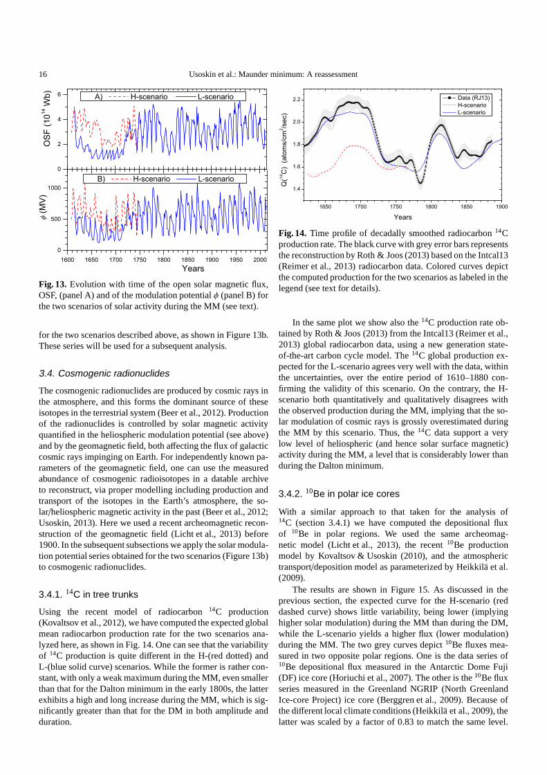
16 Usoskin et al.: Maunder minimum: A reassessment

0

2

4

6

1600 1650 1700 1750 1800 1850 1900 1950 2000

0

500

1000

OS

F (

10

14 W

b)

A) H-scenario L-scenario

φ (

MV

)

Years

B) H-scenario L-scenario

Fig. 13. Evolution with time of the open solar magnetic flux,OSF, (panel A) and of the modulation potentialφ (panel B) forthe two scenarios of solar activity during the MM (see text).

for the two scenarios described above, as shown in Figure 13b.These series will be used for a subsequent analysis.

3.4. Cosmogenic radionuclides

The cosmogenic radionuclides are produced by cosmic rays inthe atmosphere, and this forms the dominant source of theseisotopes in the terrestrial system (Beer et al., 2012). Productionof the radionuclides is controlled by solar magnetic activityquantified in the heliospheric modulation potential (see above)and by the geomagnetic field, both affecting the flux of galacticcosmic rays impinging on Earth. For independently known pa-rameters of the geomagnetic field, one can use the measuredabundance of cosmogenic radioisotopes in a datable archiveto reconstruct, via proper modelling including productionandtransport of the isotopes in the Earth’s atmosphere, the so-lar/heliospheric magnetic activity in the past (Beer et al., 2012;Usoskin, 2013). Here we used a recent archeomagnetic recon-struction of the geomagnetic field (Licht et al., 2013) before1900. In the subsequent subsections we apply the solar modula-tion potential series obtained for the two scenarios (Figure 13b)to cosmogenic radionuclides.

3.4.1. 14C in tree trunks

Using the recent model of radiocarbon14C production(Kovaltsov et al., 2012), we have computed the expected globalmean radiocarbon production rate for the two scenarios ana-lyzed here, as shown in Fig. 14. One can see that the variabilityof 14C production is quite different in the H-(red dotted) andL-(blue solid curve) scenarios. While the former is rather con-stant, with only a weak maximum during the MM, even smallerthan that for the Dalton minimum in the early 1800s, the latterexhibits a high and long increase during the MM, which is sig-nificantly greater than that for the DM in both amplitude andduration.

1650 1700 1750 1800 1850 1900

1.4

1.6

1.8

2.0

2.2 Data (RJ13)

H-scenario

L-scenario

Q(1

4C

) (

ato

ms/c

m2/s

ec)

Years

Fig. 14. Time profile of decadally smoothed radiocarbon14Cproduction rate. The black curve with grey error bars representsthe reconstruction by Roth & Joos (2013) based on the Intcal13(Reimer et al., 2013) radiocarbon data. Colored curves depictthe computed production for the two scenarios as labeled in thelegend (see text for details).

In the same plot we show also the14C production rate ob-tained by Roth & Joos (2013) from the Intcal13 (Reimer et al.,2013) global radiocarbon data, using a new generation state-of-the-art carbon cycle model. The14C global production ex-pected for the L-scenario agrees very well with the data, withinthe uncertainties, over the entire period of 1610–1880 con-firming the validity of this scenario. On the contrary, the H-scenario both quantitatively and qualitatively disagreeswiththe observed production during the MM, implying that the so-lar modulation of cosmic rays is grossly overestimated duringthe MM by this scenario. Thus, the14C data support a verylow level of heliospheric (and hence solar surface magnetic)activity during the MM, a level that is considerably lower thanduring the Dalton minimum.

3.4.2. 10Be in polar ice cores

With a similar approach to that taken for the analysis of14C (section 3.4.1) we have computed the depositional fluxof 10Be in polar regions. We used the same archeomag-netic model (Licht et al., 2013), the recent10Be productionmodel by Kovaltsov & Usoskin (2010), and the atmospherictransport/deposition model as parameterized by Heikkila et al.(2009).

The results are shown in Figure 15. As discussed in theprevious section, the expected curve for the H-scenario (reddashed curve) shows little variability, being lower (implyinghigher solar modulation) during the MM than during the DM,while the L-scenario yields a higher flux (lower modulation)during the MM. The two grey curves depict10Be fluxes mea-sured in two opposite polar regions. One is the data series of10Be depositional flux measured in the Antarctic Dome Fuji(DF) ice core (Horiuchi et al., 2007). The other is the10Be fluxseries measured in the Greenland NGRIP (North GreenlandIce-core Project) ice core (Berggren et al., 2009). Becauseofthe different local climate conditions (Heikkila et al., 2009), thelatter was scaled by a factor of 0.83 to match the same level.

Usoskin et al.: Maunder minimum: A reassessment 17

1650 1700 1750 1800 1850 1900

0.006

0.008

0.010

0.012

10B

e flu

x (

at/cm

2/s

ec)

Years

DF NGRIP x0.83

L- H-scenario

Fig. 15. Depositional flux of10Be in polar ice. All data arepseudo-decadal and≈ 25-yr smoothed because of strong high-frequency noise. Grey curves depict the fluxes measured atDome Fuji (DF) in Antarctica (Horiuchi et al., 2007), and atNGRIP (scaled as 0.83), Greenland (Berggren et al., 2009).Error bars are estimates of both statistical and systematicer-rors. The blue and red curves depict the modelled10Be depo-sitional fluxes for the L- and H-scenarios (see text for details),respectively.

This scaling does not affect the shape of the curve and in par-ticular not the ratio of the10Be flux in the MM and the DM.One can see that while the time profiles of the two datasetsdiffer in detail, probably because of the different climate pat-terns (Usoskin et al., 2009a) and/or timing uncertainties, bothyield high 10Be production during the MM. This correspondsto extremely low solar activity (McCracken et al., 2004). TheL-scenario agrees with the data reasonably well (the data dis-play even higher maxima than the model), while the H-scenarioclearly fails to reproduce the variability of10Be measured inpolar ice.

Thus, the10Be data from both Antarctic and Greenland icecores support a very low level of heliospheric (and hence solarsurface magnetic) activity during the MM, significantly lowerthan during the Dalton minimum.

3.4.3. 44Ti in meteorites

While records of terrestrial cosmogenic radionuclides maybe affected by transport and deposition processes, which arenot always exactly known (Usoskin et al., 2009a; Beer et al.,2012), cosmogenic nuclides measured in fallen meteorites arefree of this uncertainty, since the nuclides are produced di-rectly in the meteorite’s body while in space, and measuredafter their fall on the Earth. However, time resolution is lost orat least greatly reduced in this case, and the measured activ-ity represents a balance between production and decay over thetime before the fall of the meteorite. An ideal cosmogenic nu-clide for our purpose is44Ti with a half-life of about 60 years(Ahmad et al., 1998; Bonino et al., 1995). Here we test the cos-mic ray variability as inferred from different scenarios of solaractivity since 1600, following exactly the method described indetail in Usoskin et al. (2006) and the dataset of44Ti activitymeasured in 19 stony meteorites fallen between 1776 and 2001(Taricco et al., 2006). Applying the modulation potential series

1700 1750 1800 1850 1900 1950 2000

4

6

8

10 H-scenario

L-scenario

44T

i activity (

dpm

/kg Fe+Ni)

Years

Fig. 16. Time profile of the44Ti activity in units of disintegra-tions per minute per kg of iron and nickel in the meteorite. Thegrey dots with error bars are the measurements (Taricco et al.,2006). The colored curves depict the computed activity for thetwo scenarios (see text).

as described in Sect. 3.3 to the cosmic ray flux and calculat-ing the expected44Ti activity as a function of the time of themeteorite’s fall, we compare the model computations for thetwo scenarios with the measured values in Fig. 16. One cansee that the series for the L-scenario fits the data rather well,whereas the curve resulting from the H-scenario lies consider-ably too low. As a merit parameter of the agreement we use theχ2 value for the period of 3.3 half-lives (attenuation factor 10)since the middle of the MM, viz. until 1880, which includes7 meteorites fallen between 1776 and 1869 (7 degrees of free-dom). Theχ2(7) for the L-scenario is 2 (0.33 per degree of free-dom), which perfectly fits the hypothesis. For the H-scenario,however,χ2(7) = 17.6 (2.93 per degree of freedom) indicat-ing that this hypothesis should be rejected with a high signifi-cance of 0.014. Note that the long residence times of the me-teorites within the helisophere means that the difference duringthe MM between the two scenarios has an influence on the pre-dicted44Ti abundances even for meteorites that fell to Earth rel-atively recently. This results in the observed abundances beinginconsistent with the H-scenario for a large number of the me-teorites whereas they are consistent, within the observationaluncertainty, with the L-scenario.

Accordingly, the hypothesis of a high level of solar activ-ity during the MM is rejected at a high significance level usingindirect data of44Ti in meteorites, while the conventional sce-nario of very low activity during the MM is in full agreementwith the data.

4. Consequences of the Maunder minimum

4.1. Solar/stellar dynamo

Major changes in the secular level of solar activity, such asGrand minima/maxima form a challenge for our understand-ing of the origin and evolution of the solar magnetic field.It has been recently shown, by analyzing the sunspot num-bers reconstructed from14C for the last 3000 years, that Grandminima form a separate mode of solar activity (Usoskin et al.,2014), likely corresponding to a special regime of the solardy-namo. In addition to the traditional concept of cyclic solarac-

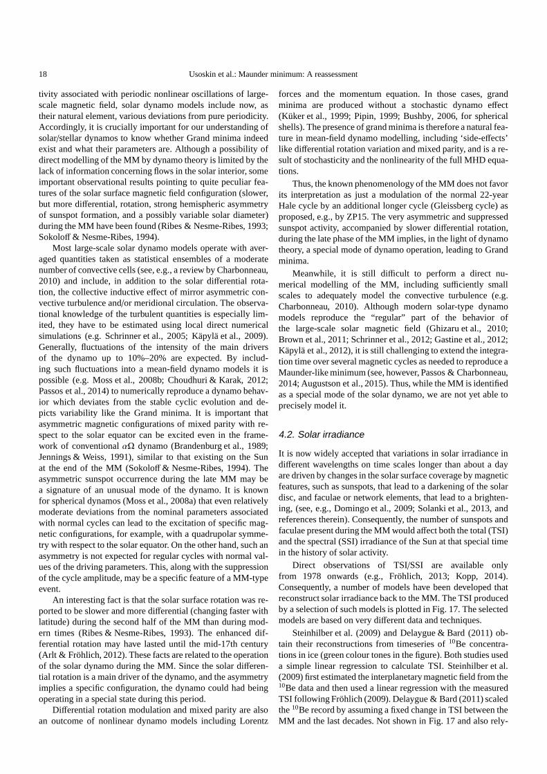
18 Usoskin et al.: Maunder minimum: A reassessment

tivity associated with periodic nonlinear oscillations oflarge-scale magnetic field, solar dynamo models include now, astheir natural element, various deviations from pure periodicity.Accordingly, it is crucially important for our understanding ofsolar/stellar dynamos to know whether Grand minima indeedexist and what their parameters are. Although a possibilityofdirect modelling of the MM by dynamo theory is limited by thelack of information concerning flows in the solar interior, someimportant observational results pointing to quite peculiar fea-tures of the solar surface magnetic field configuration (slower,but more differential, rotation, strong hemispheric asymmetryof sunspot formation, and a possibly variable solar diameter)during the MM have been found (Ribes & Nesme-Ribes, 1993;Sokoloff & Nesme-Ribes, 1994).

Most large-scale solar dynamo models operate with aver-aged quantities taken as statistical ensembles of a moderatenumber of convective cells (see, e.g., a review by Charbonneau,2010) and include, in addition to the solar differential rota-tion, the collective inductive effect of mirror asymmetric con-vective turbulence and/or meridional circulation. The observa-tional knowledge of the turbulent quantities is especiallylim-ited, they have to be estimated using local direct numericalsimulations (e.g. Schrinner et al., 2005; Kapyla et al., 2009).Generally, fluctuations of the intensity of the main driversof the dynamo up to 10%–20% are expected. By includ-ing such fluctuations into a mean-field dynamo models it ispossible (e.g. Moss et al., 2008b; Choudhuri & Karak, 2012;Passos et al., 2014) to numerically reproduce a dynamo behav-ior which deviates from the stable cyclic evolution and de-picts variability like the Grand minima. It is important thatasymmetric magnetic configurations of mixed parity with re-spect to the solar equator can be excited even in the frame-work of conventionalαΩ dynamo (Brandenburg et al., 1989;Jennings & Weiss, 1991), similar to that existing on the Sunat the end of the MM (Sokoloff & Nesme-Ribes, 1994). Theasymmetric sunspot occurrence during the late MM may bea signature of an unusual mode of the dynamo. It is knownfor spherical dynamos (Moss et al., 2008a) that even relativelymoderate deviations from the nominal parameters associatedwith normal cycles can lead to the excitation of specific mag-netic configurations, for example, with a quadrupolar symme-try with respect to the solar equator. On the other hand, suchanasymmetry is not expected for regular cycles with normal val-ues of the driving parameters. This, along with the suppressionof the cycle amplitude, may be a specific feature of a MM-typeevent.

An interesting fact is that the solar surface rotation was re-ported to be slower and more differential (changing faster withlatitude) during the second half of the MM than during mod-ern times (Ribes & Nesme-Ribes, 1993). The enhanced dif-ferential rotation may have lasted until the mid-17th century(Arlt & Frohlich, 2012). These facts are related to the operationof the solar dynamo during the MM. Since the solar differen-tial rotation is a main driver of the dynamo, and the asymmetryimplies a specific configuration, the dynamo could had beingoperating in a special state during this period.

Differential rotation modulation and mixed parity are alsoan outcome of nonlinear dynamo models including Lorentz

forces and the momentum equation. In those cases, grandminima are produced without a stochastic dynamo effect(Kuker et al., 1999; Pipin, 1999; Bushby, 2006, for sphericalshells). The presence of grand minima is therefore a naturalfea-ture in mean-field dynamo modelling, including ‘side-effects’like differential rotation variation and mixed parity, and is a re-sult of stochasticity and the nonlinearity of the full MHD equa-tions.

Thus, the known phenomenology of the MM does not favorits interpretation as just a modulation of the normal 22-yearHale cycle by an additional longer cycle (Gleissberg cycle)asproposed, e.g., by ZP15. The very asymmetric and suppressedsunspot activity, accompanied by slower differential rotation,during the late phase of the MM implies, in the light of dynamotheory, a special mode of dynamo operation, leading to Grandminima.

Meanwhile, it is still difficult to perform a direct nu-merical modelling of the MM, including sufficiently smallscales to adequately model the convective turbulence (e.g.Charbonneau, 2010). Although modern solar-type dynamomodels reproduce the “regular” part of the behavior ofthe large-scale solar magnetic field (Ghizaru et al., 2010;Brown et al., 2011; Schrinner et al., 2012; Gastine et al., 2012;Kapyla et al., 2012), it is still challenging to extend theintegra-tion time over several magnetic cycles as needed to reproduce aMaunder-like minimum (see, however, Passos & Charbonneau,2014; Augustson et al., 2015). Thus, while the MM is identifiedas a special mode of the solar dynamo, we are not yet able toprecisely model it.

4.2. Solar irradiance

It is now widely accepted that variations in solar irradiance indifferent wavelengths on time scales longer than about a dayare driven by changes in the solar surface coverage by magneticfeatures, such as sunspots, that lead to a darkening of the solardisc, and faculae or network elements, that lead to a brighten-ing, (see, e.g., Domingo et al., 2009; Solanki et al., 2013, andreferences therein). Consequently, the number of sunspotsandfaculae present during the MM would affect both the total (TSI)and the spectral (SSI) irradiance of the Sun at that special timein the history of solar activity.

Direct observations of TSI/SSI are available onlyfrom 1978 onwards (e.g., Frohlich, 2013; Kopp, 2014).Consequently, a number of models have been developed thatreconstruct solar irradiance back to the MM. The TSI producedby a selection of such models is plotted in Fig. 17. The selectedmodels are based on very different data and techniques.

Steinhilber et al. (2009) and Delaygue & Bard (2011) ob-tain their reconstructions from timeseries of10Be concentra-tions in ice (green colour tones in the figure). Both studies useda simple linear regression to calculate TSI. Steinhilber etal.(2009) first estimated the interplanetary magnetic field from the10Be data and then used a linear regression with the measuredTSI following Frohlich (2009). Delaygue & Bard (2011) scaledthe10Be record by assuming a fixed change in TSI between theMM and the last decades. Not shown in Fig. 17 and also rely-

Usoskin et al.: Maunder minimum: A reassessment 19

Fig. 17. Selected TSI reconstructions since 1600, labeledin the plot are: Sea09 –Steinhilber et al. (2009); DB11 –Delaygue & Bard (2011); Wea05 – Wang et al. (2005); Kea10– Krivova et al. (2010); Dea14 – Dasi-Espuig et al. (2014);Vea11 – Vieira et al. (2011). The green, blue and red colourtones are used for the reconstructions based on the10Be,sunspot and14C data, respectively. The black dotted line marksthe TSI value at modern solar activity minimum conditions ac-cording to SORCE/TIM measurements.

ing on the10Be data is the TSI reconstruction by Shapiro et al.(2011). The magnitude of the secular change in this modelcomes from the difference between semi-empirical model at-mospheres describing the darkest parts of the solar surfaceand the average quiet Sun (during modern times). The secu-lar change thus obtained is significantly higher than in all othermodels (3 W m−2 even after the re-assessment by Judge et al.2012). However, the shape of the secular change comes againfrom a linear regression to the10Be record, so that it is essen-tially the same as in the other two models using10Be concen-trations.

Blue color tones show reconstructions that employ morephysics-based approaches and are build on the sunspot number.Wang et al. (2005) reconstructed the TSI from the magneticflux evolved by a flux transport simulation (Sheeley, 2005).Krivova et al. (2010) employed the approach of Solanki et al.(2002) to compute the magnetic flux from the sunspot num-ber and therefrom the technique of Krivova et al. (2007) tocompute the TSI and the spectral irradiance. Dasi-Espuig etal.(2014) used a flux transport model (Jiang et al., 2010, 2011b)to simulate solar magnetograms to which they applied theSATIRE-S model (Fligge et al., 2000; Krivova et al., 2003).

Finally, Vieira et al. (2011) adapted the models bySolanki et al. (2002) and Krivova et al. (2007) for use with14Cdata (red color tones). The red lines show reconstructions byVieira et al. (2011) based on two different models of the geo-magnetic field. They hardly diverge over the considered period.

The magnitude of the secular increase in the TSI since theMM differs by roughly 0.5 W m−2 between the models shownin the figure. The full range of this variation is actually con-siderably larger, since the change obtained by Shapiro et al.

2011, in the correction proposed by Judge et al. 2012, is about3 W m−2. More important for the purposes of the present pa-per is that despite this quantitative difference, the trends shownby all reconstructions are qualitatively similar. In otherwords,quite irrespective of the data or the technique used for theTSI reconstruction, the TSI is always lower during the MMthan during the Dalton minimum by on average 0.2–0.3 W m−2

(more for the model by Shapiro et al. 2011). This appears to bea rather robust feature. If the sunspot number during the MMwere as high as proposed by ZP15 then this difference wouldvanish. This contradicts all TSI reconstructions, including onesthat are not built on sunspot numbers at all, although the un-certainties in the TSI reconstructions are sufficiently large thatthis cannot be judged to be a very stong constraint (and is notentirely independent of the other arguments provided in thispaper).

5. Conclusions

We have revisited the level of solar activity during the Maunderminimum, using all the existing, both direct and indirect,datasets and evidence to show that the activity was very low,significantly lower than during the Dalton minimum or the cur-rent weak solar cycle # 24. We have confronted the data avail-able with two scenarios of the solar activity level during theMM – the low activity (L-scenario) and the high activity (H-scenario, see Sect. 2).

The results can be summarized as follows:We have evaluated (Sect. 2.1), using a conservative ap-

proach, the fraction of sunspot active days during the MM. Thefraction appeared small, implying a very low level of sunspotactivity.

We have revisited (Sect. 2.2) the telescopic solar observa-tions during the MM and we conclude that the astronomers ofthe 17th century, especially in its second half, were very un-likely to be influenced by the religious or philosophical dog-mas. This is contrary to the claim by ZP15.

We have discussed that the short gaps in the HS98 database,which were interpreted by ZP15 as deliberate omission ofsunspot records by the 17th century observers for non-scientificreasons, are caused by a technical artefact of the database com-pilation and do not correspond to observational lacunas.

We have pointed out (Sect. 2.4) outdated and erroneousinformation and serious methodological flaws in the analysisdone by ZP15 that led them to severely overestimate the solaractivity level during the MM.

The latitudinal extent of sunspot formation (Sect. 2.5) alsopoints to a very low solar activity during the MM.

We have shown (Sect. 2.6) that East-Asian naked-eyesunspot observations cannot be used to assess the exact levelof solar activity. The existing data do not contradict to theverylow activity level during the MM.

We have presented a re-analysis of several documentedsources, some new to science so far, on the occurrence of lower-latitude aurorae on Earth. We have demonstrated that the MMindeed displayed very low activity also in terms of auroralsightings (Sect. 3.1) compared to normal periods and also tothe Dalton minimum.

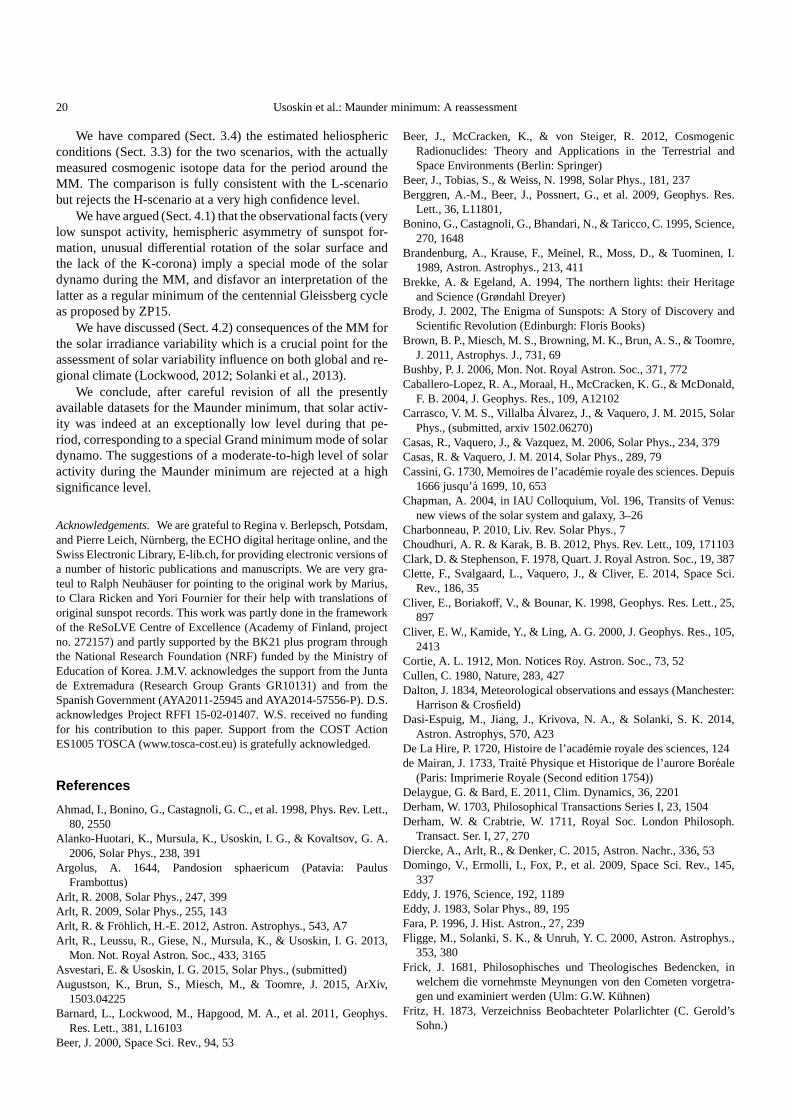
20 Usoskin et al.: Maunder minimum: A reassessment

We have compared (Sect. 3.4) the estimated heliosphericconditions (Sect. 3.3) for the two scenarios, with the actuallymeasured cosmogenic isotope data for the period around theMM. The comparison is fully consistent with the L-scenariobut rejects the H-scenario at a very high confidence level.

We have argued (Sect. 4.1) that the observational facts (verylow sunspot activity, hemispheric asymmetry of sunspot for-mation, unusual differential rotation of the solar surface andthe lack of the K-corona) imply a special mode of the solardynamo during the MM, and disfavor an interpretation of thelatter as a regular minimum of the centennial Gleissberg cycleas proposed by ZP15.

We have discussed (Sect. 4.2) consequences of the MM forthe solar irradiance variability which is a crucial point for theassessment of solar variability influence on both global andre-gional climate (Lockwood, 2012; Solanki et al., 2013).

We conclude, after careful revision of all the presentlyavailable datasets for the Maunder minimum, that solar activ-ity was indeed at an exceptionally low level during that pe-riod, corresponding to a special Grand minimum mode of solardynamo. The suggestions of a moderate-to-high level of solaractivity during the Maunder minimum are rejected at a highsignificance level.

Acknowledgements. We are grateful to Regina v. Berlepsch, Potsdam,and Pierre Leich, Nurnberg, the ECHO digital heritage online, and theSwiss Electronic Library, E-lib.ch, for providing electronic versions ofa number of historic publications and manuscripts. We are very gra-teul to Ralph Neuhauser for pointing to the original work byMarius,to Clara Ricken and Yori Fournier for their help with translations oforiginal sunspot records. This work was partly done in the frameworkof the ReSoLVE Centre of Excellence (Academy of Finland, projectno. 272157) and partly supported by the BK21 plus program throughthe National Research Foundation (NRF) funded by the Ministry ofEducation of Korea. J.M.V. acknowledges the support from the Juntade Extremadura (Research Group Grants GR10131) and from theSpanish Government (AYA2011-25945 and AYA2014-57556-P).D.S.acknowledges Project RFFI 15-02-01407. W.S. received no fundingfor his contribution to this paper. Support from the COST ActionES1005 TOSCA (www.tosca-cost.eu) is gratefully acknowledged.

References

Ahmad, I., Bonino, G., Castagnoli, G. C., et al. 1998, Phys. Rev. Lett.,80, 2550

Alanko-Huotari, K., Mursula, K., Usoskin, I. G., & Kovaltsov, G. A.2006, Solar Phys., 238, 391

Argolus, A. 1644, Pandosion sphaericum (Patavia: PaulusFrambottus)

Arlt, R. 2008, Solar Phys., 247, 399Arlt, R. 2009, Solar Phys., 255, 143Arlt, R. & Frohlich, H.-E. 2012, Astron. Astrophys., 543, A7Arlt, R., Leussu, R., Giese, N., Mursula, K., & Usoskin, I. G.2013,

Mon. Not. Royal Astron. Soc., 433, 3165Asvestari, E. & Usoskin, I. G. 2015, Solar Phys., (submitted)Augustson, K., Brun, S., Miesch, M., & Toomre, J. 2015, ArXiv,

1503.04225Barnard, L., Lockwood, M., Hapgood, M. A., et al. 2011, Geophys.

Res. Lett., 381, L16103Beer, J. 2000, Space Sci. Rev., 94, 53

Beer, J., McCracken, K., & von Steiger, R. 2012, CosmogenicRadionuclides: Theory and Applications in the TerrestrialandSpace Environments (Berlin: Springer)

Beer, J., Tobias, S., & Weiss, N. 1998, Solar Phys., 181, 237Berggren, A.-M., Beer, J., Possnert, G., et al. 2009, Geophys. Res.

Lett., 36, L11801,Bonino, G., Castagnoli, G., Bhandari, N., & Taricco, C. 1995, Science,

270, 1648Brandenburg, A., Krause, F., Meinel, R., Moss, D., & Tuominen, I.

1989, Astron. Astrophys., 213, 411Brekke, A. & Egeland, A. 1994, The northern lights: their Heritage

and Science (Grøndahl Dreyer)Brody, J. 2002, The Enigma of Sunspots: A Story of Discovery and

Scientific Revolution (Edinburgh: Floris Books)Brown, B. P., Miesch, M. S., Browning, M. K., Brun, A. S., & Toomre,

J. 2011, Astrophys. J., 731, 69Bushby, P. J. 2006, Mon. Not. Royal Astron. Soc., 371, 772Caballero-Lopez, R. A., Moraal, H., McCracken, K. G., & McDonald,

F. B. 2004, J. Geophys. Res., 109, A12102Carrasco, V. M. S., VillalbaAlvarez, J., & Vaquero, J. M. 2015, Solar

Phys., (submitted, arxiv 1502.06270)Casas, R., Vaquero, J., & Vazquez, M. 2006, Solar Phys., 234,379Casas, R. & Vaquero, J. M. 2014, Solar Phys., 289, 79Cassini, G. 1730, Memoires de l’academie royale des sciences. Depuis

1666 jusqu’a 1699, 10, 653Chapman, A. 2004, in IAU Colloquium, Vol. 196, Transits of Venus:

new views of the solar system and galaxy, 3–26Charbonneau, P. 2010, Liv. Rev. Solar Phys., 7Choudhuri, A. R. & Karak, B. B. 2012, Phys. Rev. Lett., 109, 171103Clark, D. & Stephenson, F. 1978, Quart. J. Royal Astron. Soc., 19, 387Clette, F., Svalgaard, L., Vaquero, J., & Cliver, E. 2014, Space Sci.

Rev., 186, 35Cliver, E., Boriakoff, V., & Bounar, K. 1998, Geophys. Res. Lett., 25,

897Cliver, E. W., Kamide, Y., & Ling, A. G. 2000, J. Geophys. Res., 105,

2413Cortie, A. L. 1912, Mon. Notices Roy. Astron. Soc., 73, 52Cullen, C. 1980, Nature, 283, 427Dalton, J. 1834, Meteorological observations and essays (Manchester:

Harrison & Crosfield)Dasi-Espuig, M., Jiang, J., Krivova, N. A., & Solanki, S. K. 2014,

Astron. Astrophys, 570, A23De La Hire, P. 1720, Histoire de l’academie royale des sciences, 124de Mairan, J. 1733, Traite Physique et Historique de l’aurore Boreale

(Paris: Imprimerie Royale (Second edition 1754))Delaygue, G. & Bard, E. 2011, Clim. Dynamics, 36, 2201Derham, W. 1703, Philosophical Transactions Series I, 23, 1504Derham, W. & Crabtrie, W. 1711, Royal Soc. London Philosoph.

Transact. Ser. I, 27, 270Diercke, A., Arlt, R., & Denker, C. 2015, Astron. Nachr., 336, 53Domingo, V., Ermolli, I., Fox, P., et al. 2009, Space Sci. Rev., 145,

337Eddy, J. 1976, Science, 192, 1189Eddy, J. 1983, Solar Phys., 89, 195Fara, P. 1996, J. Hist. Astron., 27, 239Fligge, M., Solanki, S. K., & Unruh, Y. C. 2000, Astron. Astrophys.,

353, 380Frick, J. 1681, Philosophisches und Theologisches Bedencken, in

welchem die vornehmste Meynungen von den Cometen vorgetra-gen und examiniert werden (Ulm: G.W. Kuhnen)

Fritz, H. 1873, Verzeichniss Beobachteter Polarlichter (C. Gerold’sSohn.)

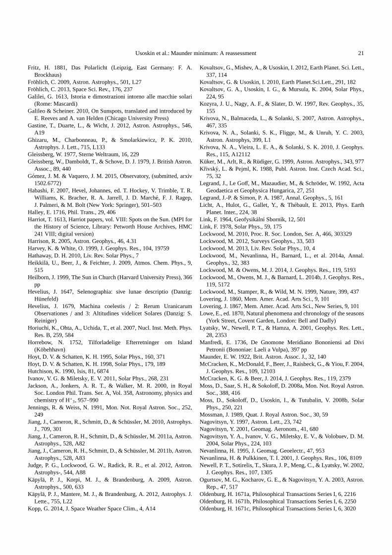
Usoskin et al.: Maunder minimum: A reassessment 21

Fritz, H. 1881, Das Polarlicht (Leipzig, East Germany: F. A.Brockhaus)

Frohlich, C. 2009, Astron. Astrophys., 501, L27Frohlich, C. 2013, Space Sci. Rev., 176, 237Galilei, G. 1613, Istoria e dimostrazioni intorno alle macchie solari

(Rome: Mascardi)Galileo & Scheiner. 2010, On Sunspots, translated and introduced by

E. Reeves and A. van Helden (Chicago University Press)Gastine, T., Duarte, L., & Wicht, J. 2012, Astron. Astrophys., 546,

A19Ghizaru, M., Charbonneau, P., & Smolarkiewicz, P. K. 2010,

Astrophys. J. Lett., 715, L133Gleissberg, W. 1977, Sterne Weltraum, 16, 229Gleissberg, W., Damboldt, T., & Schove, D. J. 1979, J. British Astron.

Assoc., 89, 440Gomez, J. M. & Vaquero, J. M. 2015, Observatory, (submitted, arxiv

1502.6772)Habashi, F. 2007, Hevel, Johannes, ed. T. Hockey, V. Trimble, T. R.

Williams, K. Bracher, R. A. Jarrell, J. D. Marche, F. J. Ragep,J. Palmeri, & M. Bolt (New York: Springer), 501–503

Halley, E. 1716, Phil. Trans., 29, 406Harriot, T. 1613, Harriot papers, vol. VIII: Spots on the Sun. (MPI for

the History of Science, Library: Petworth House Archives, HMC241 VIII; digital version)

Harrison, R. 2005, Astron. Geophys., 46, 4.31Harvey, K. & White, O. 1999, J. Geophys. Res., 104, 19759Hathaway, D. H. 2010, Liv. Rev. Solar Phys., 7Heikkila, U., Beer, J., & Feichter, J. 2009, Atmos. Chem. Phys., 9,

515Heilborn, J. 1999, The Sun in Church (Harvard University Press), 366

ppHevelius, J. 1647, Selenographia: sive lunae descriptio (Danzig:

Hunefeld)Hevelius, J. 1679, Machina coelestis/ 2: Rerum Uranicarum

Observationes/ and 3: Altitudines videlicet Solares (Danzig: S.Reiniger)

Horiuchi, K., Ohta, A., Uchida, T., et al. 2007, Nucl. Inst. Meth. Phys.Res. B, 259, 584

Horrebow, N. 1752, Tilforladelige Efterretninger om Island(Kobehhavn)

Hoyt, D. V. & Schatten, K. H. 1995, Solar Phys., 160, 371Hoyt, D. V. & Schatten, K. H. 1998, Solar Phys., 179, 189Hutchison, K. 1990, Isis, 81, 6874Ivanov, V. G. & Miletsky, E. V. 2011, Solar Phys., 268, 231Jackson, A., Jonkers, A. R. T., & Walker, M. R. 2000, in Royal

Soc. London Phil. Trans. Ser. A, Vol. 358, Astronomy, physics andchemistry of H+3, 957–990

Jennings, R. & Weiss, N. 1991, Mon. Not. Royal Astron. Soc., 252,249

Jiang, J., Cameron, R., Schmitt, D., & Schussler, M. 2010, Astrophys.J., 709, 301

Jiang, J., Cameron, R. H., Schmitt, D., & Schussler, M. 2011a, Astron.Astrophys., 528, A82

Jiang, J., Cameron, R. H., Schmitt, D., & Schussler, M. 2011b, Astron.Astrophys., 528, A83

Judge, P. G., Lockwood, G. W., Radick, R. R., et al. 2012, Astron.Astrophys-, 544, A88

Kapyla, P. J., Korpi, M. J., & Brandenburg, A. 2009, Astron.Astrophys., 500, 633

Kapyla, P. J., Mantere, M. J., & Brandenburg, A. 2012, Astrophys. J.Lette., 755, L22

Kopp, G. 2014, J. Space Weather Space Clim., 4, A14

Kovaltsov, G., Mishev, A., & Usoskin, I. 2012, Earth Planet.Sci. Lett.,337, 114

Kovaltsov, G. & Usoskin, I. 2010, Earth Planet.Sci.Lett., 291, 182Kovaltsov, G. A., Usoskin, I. G., & Mursula, K. 2004, Solar Phys.,

224, 95Kozyra, J. U., Nagy, A. F., & Slater, D. W. 1997, Rev. Geophys., 35,

155Krivova, N., Balmaceda, L., & Solanki, S. 2007, Astron. Astrophys.,

467, 335Krivova, N. A., Solanki, S. K., Fligge, M., & Unruh, Y. C. 2003,

Astron. Astrophys, 399, L1Krivova, N. A., Vieira, L. E. A., & Solanki, S. K. 2010, J. Geophys.

Res., 115, A12112Kuker, M., Arlt, R., & Rudiger, G. 1999, Astron. Astrophys., 343, 977Krivsky, L. & Pejml, K. 1988, Publ. Astron. Inst. Czech Acad. Sci.,

75, 32Legrand, J., Le Goff, M., Mazaudier, M., & Schroder, W. 1992, Acta

Geodaetica et Geophysica Hungarica, 27, 251Legrand, J.-P. & Simon, P. A. 1987, Annal. Geophys., 5, 161Licht, A., Hulot, G., Gallet, Y., & Thebault, E. 2013, Phys.Earth

Planet. Inter., 224, 38Link, F. 1964, Geofysikalnı Sbornık, 12, 501Link, F. 1978, Solar Phys., 59, 175Lockwood, M. 2010, Proc. R. Soc. London, Ser. A, 466, 303329Lockwood, M. 2012, Surveys Geophys., 33, 503Lockwood, M. 2013, Liv. Rev. Solar Phys., 10, 4Lockwood, M., Nevanlinna, H., Barnard, L., et al. 2014a, Annal.

Geophys., 32, 383Lockwood, M. & Owens, M. J. 2014, J. Geophys. Res., 119, 5193Lockwood, M., Owens, M. J., & Barnard, L. 2014b, J. Geophys. Res.,

119, 5172Lockwood, M., Stamper, R., & Wild, M. N. 1999, Nature, 399, 437Lovering, J. 1860, Mem. Amer. Acad. Arts Sci., 9, 101Lovering, J. 1867, Mem. Amer. Acad. Arts Sci., New Series, 9,101Lowe, E., ed. 1870, Natural phenomena and chronology of the seasons

(York Street, Covent Garden, London: Bell and Dadly)Lyatsky, W., Newell, P. T., & Hamza, A. 2001, Geophys. Res. Lett.,

28, 2353Manfredi, E. 1736, De Gnomone Meridiano Bononiensi ad Divi

Petronii (Bononiae: Laeli a Vulpa), 397 ppMaunder, E. W. 1922, Brit. Astron. Assoc. J., 32, 140McCracken, K., McDonald, F., Beer, J., Raisbeck, G., & Yiou,F. 2004,

J. Geophys. Res., 109, 12103McCracken, K. G. & Beer, J. 2014, J. Geophys. Res., 119, 2379Moss, D., Saar, S. H., & Sokoloff, D. 2008a, Mon. Not. Royal Astron.

Soc., 388, 416Moss, D., Sokoloff, D., Usoskin, I., & Tutubalin, V. 2008b, Solar

Phys., 250, 221Mossman, J. 1989, Quat. J. Royal Astron. Soc., 30, 59Nagovitsyn, Y. 1997, Astron. Lett., 23, 742Nagovitsyn, Y. 2001, Geomag. Aeronom., 41, 680Nagovitsyn, Y. A., Ivanov, V. G., Miletsky, E. V., & Volobuev, D. M.

2004, Solar Phys., 224, 103Nevanlinna, H. 1995, J. Geomag. Geoelectr., 47, 953Nevanlinna, H. & Pulkkinen, T. I. 2001, J. Geophys. Res., 106, 8109Newell, P. T., Sotirelis, T., Skura, J. P., Meng, C., & Lyatsky, W. 2002,

J. Geophys. Res., 107, 1305Ogurtsov, M. G., Kocharov, G. E., & Nagovitsyn, Y. A. 2003, Astron.

Rep., 47, 517Oldenburg, H. 1671a, Philosophical Transactions Series I,6, 2216Oldenburg, H. 1671b, Philosophical Transactions Series I,6, 2250Oldenburg, H. 1671c, Philosophical Transactions Series I,6, 3020

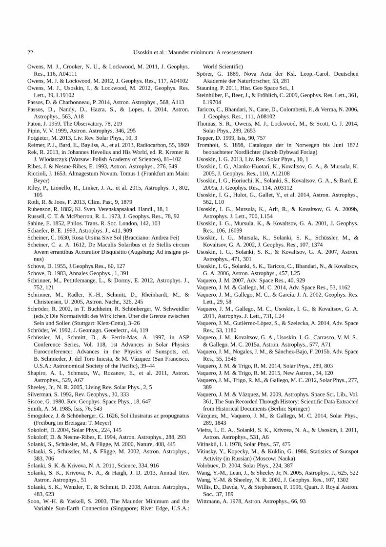
22 Usoskin et al.: Maunder minimum: A reassessment

Owens, M. J., Crooker, N. U., & Lockwood, M. 2011, J. Geophys.Res., 116, A04111

Owens, M. J. & Lockwood, M. 2012, J. Geophys. Res., 117, A04102Owens, M. J., Usoskin, I., & Lockwood, M. 2012, Geophys. Res.

Lett., 39, L19102Passos, D. & Charbonneau, P. 2014, Astron. Astrophys., 568,A113Passos, D., Nandy, D., Hazra, S., & Lopes, I. 2014, Astron.

Astrophys., 563, A18Paton, J. 1959, The Observatory, 78, 219Pipin, V. V. 1999, Astron. Astrophys, 346, 295Potgieter, M. 2013, Liv. Rev. Solar Phys., 10, 3Reimer, P. J., Bard, E., Bayliss, A., et al. 2013, Radiocarbon, 55, 1869Rek, R. 2013, in Johannes Hevelius and His World, ed. R. Kremer &

J. Wlodarczyk (Warsaw: Polish Academy of Sciences), 81–102Ribes, J. & Nesme-Ribes, E. 1993, Astron. Astrophys., 276, 549Riccioli, J. 1653, Almagestum Novum. Tomus 1 (Frankfurt am Main:

Beyer)Riley, P., Lionello, R., Linker, J. A., et al. 2015, Astrophys. J., 802,

105Roth, R. & Joos, F. 2013, Clim. Past, 9, 1879Rubenson, R. 1882, Kl. Sven. Vetenskapsakad. Handl., 18, 1Russell, C. T. & McPherron, R. L. 1973, J. Geophys. Res., 78, 92Sabine, E. 1852, Philos. Trans. R. Soc. London, 142, 103Schaefer, B. E. 1993, Astrophys. J., 411, 909Scheiner, C. 1630, Rosa Ursina Sive Sol (Bracciano: Andrea Fei)Scheiner, C. a. A. 1612, De Maculis Solaribus et de Stellis circum

Jovem errantibus Accuratior Disquisitio (Augsburg: Ad insigne pi-nus)

Schove, D. 1955, J.Geophys.Res., 60, 127Schove, D. 1983, Annales Geophys., 1, 391Schrinner, M., Petitdemange, L., & Dormy, E. 2012, Astrophys. J.,

752, 121Schrinner, M., Radler, K.-H., Schmitt, D., Rheinhardt, M., &

Christensen, U. 2005, Astron. Nachr., 326, 245Schroder, R. 2002, in T. Buchheim, R. Schonberger, W. Schweidler

(eds.): Die Normativitat des Wirklichen.Uber die Grenze zwischenSein und Sollen (Stuttgart: Klett-Cotta), 3–26

Schroder, W. 1992, J. Geomagn. Geoelectr., 44, 119Schussler, M., Schmitt, D., & Ferriz-Mas, A. 1997, in ASP

Conference Series, Vol. 118, 1st Advances in Solar PhysicsEuroconference: Advances in the Physics of Sunspots, ed.B. Schmieder, J. del Toro Iniesta, & M. Vazquez (San Francisco,U.S.A.: Astronomical Society of the Pacific), 39–44

Shapiro, A. I., Schmutz, W., Rozanov, E., et al. 2011, Astron.Astrophys., 529, A67

Sheeley, Jr., N. R. 2005, Living Rev. Solar Phys., 2, 5Silverman, S. 1992, Rev. Geophys., 30, 333Siscoe, G. 1980, Rev. Geophys. Space Phys., 18, 647Smith, A. M. 1985, Isis, 76, 543Smogulecz, J. & Schonberger, G. 1626, Sol illustratus ac propugnatus

(Freiburg im Breisgau: T. Meyer)Sokoloff, D. 2004, Solar Phys., 224, 145Sokoloff, D. & Nesme-Ribes, E. 1994, Astron. Astrophys., 288, 293Solanki, S., Schussler, M., & Fligge, M. 2000, Nature, 408,445Solanki, S., Schussler, M., & Fligge, M. 2002, Astron. Astrophys.,

383, 706Solanki, S. K. & Krivova, N. A. 2011, Science, 334, 916Solanki, S. K., Krivova, N. A., & Haigh, J. D. 2013, Annual Rev.

Astron. Astrophys., 51Solanki, S. K., Wenzler, T., & Schmitt, D. 2008, Astron. Astrophys.,

483, 623Soon, W.-H. & Yaskell, S. 2003, The Maunder Minimum and the

Variable Sun-Earth Connection (Singapore; River Edge, U.S.A.:

World Scientific)Sporer, G. 1889, Nova Acta der Ksl. Leop.-Carol. Deutschen

Akademie der Naturforscher, 53, 281Stauning, P. 2011, Hist. Geo Space Sci., 1Steinhilber, F., Beer, J., & Frohlich, C. 2009, Geophys. Res. Lett., 361,

L19704Taricco, C., Bhandari, N., Cane, D., Colombetti, P., & Verma, N. 2006,

J. Geophys. Res., 111, A08102Thomas, S. R., Owens, M. J., Lockwood, M., & Scott, C. J. 2014,

Solar Phys., 289, 2653Topper, D. 1999, Isis, 90, 757Tromholt, S. 1898, Catalogue der in Norwegen bis Juni 1872

beobachteter Nordlichter (Jacob Dybwad Forlag)Usoskin, I. G. 2013, Liv. Rev. Solar Phys., 10, 1Usoskin, I. G., Alanko-Huotari, K., Kovaltsov, G. A., & Mursula, K.

2005, J. Geophys. Res., 110, A12108Usoskin, I. G., Horiuchi, K., Solanki, S., Kovaltsov, G. A.,& Bard, E.

2009a, J. Geophys. Res., 114, A03112Usoskin, I. G., Hulot, G., Gallet, Y., et al. 2014, Astron. Astrophys.,

562, L10Usoskin, I. G., Mursula, K., Arlt, R., & Kovaltsov, G. A. 2009b,

Astrophys. J. Lett., 700, L154Usoskin, I. G., Mursula, K., & Kovaltsov, G. A. 2001, J. Geophys.

Res., 106, 16039Usoskin, I. G., Mursula, K., Solanki, S. K., Schussler, M.,&

Kovaltsov, G. A. 2002, J. Geophys. Res., 107, 1374Usoskin, I. G., Solanki, S. K., & Kovaltsov, G. A. 2007, Astron.

Astrophys., 471, 301Usoskin, I. G., Solanki, S. K., Taricco, C., Bhandari, N., & Kovaltsov,

G. A. 2006, Astron. Astrophys., 457, L25Vaquero, J. M. 2007, Adv. Space Res., 40, 929Vaquero, J. M. & Gallego, M. C. 2014, Adv. Space Res., 53, 1162Vaquero, J. M., Gallego, M. C., & Garcıa, J. A. 2002, Geophys. Res.

Lett., 29, 58Vaquero, J. M., Gallego, M. C., Usoskin, I. G., & Kovaltsov, G. A.

2011, Astrophys. J. Lett., 731, L24Vaquero, J. M., Gutierrez-Lopez, S., & Szelecka, A. 2014,Adv. Space

Res., 53, 1180Vaquero, J. M., Kovaltsov, G. A., Usoskin, I. G., Carrasco, V. M. S.,

& Gallego, M. C. 2015a, Astron. Astrophys., 577, A71Vaquero, J. M., Nogales, J. M., & Sanchez-Bajo, F. 2015b, Adv. Space

Res., 55, 1546Vaquero, J. M. & Trigo, R. M. 2014, Solar Phys., 289, 803Vaquero, J. M. & Trigo, R. M. 2015, New Astron., 34, 120Vaquero, J. M., Trigo, R. M., & Gallego, M. C. 2012, Solar Phys., 277,

389Vaquero, J. M. & Vazquez, M. 2009, Astrophys. Space Sci. Lib., Vol.

361, The Sun Recorded Through History: Scientific Data Extractedfrom Historical Documents (Berlin: Springer)

Vazquez, M., Vaquero, J. M., & Gallego, M. C. 2014, Solar Phys.,289, 1843

Vieira, L. E. A., Solanki, S. K., Krivova, N. A., & Usoskin, I.2011,Astron. Astrophys., 531, A6

Vitinskii, I. I. 1978, Solar Phys., 57, 475Vitinsky, Y., Kopecky, M., & Kuklin, G. 1986, Statistics of Sunspot

Activity (in Russian) (Moscow: Nauka)Volobuev, D. 2004, Solar Phys., 224, 387Wang, Y.-M., Lean, J., & Sheeley Jr, N. 2005, Astrophys. J., 625, 522Wang, Y.-M. & Sheeley, N. R. 2002, J. Geophys. Res., 107, 1302Willis, D., Davda, V., & Stephenson, F. 1996, Quart. J. RoyalAstron.

Soc., 37, 189Wittmann, A. 1978, Astron. Astrophys., 66, 93

Usoskin et al.: Maunder minimum: A reassessment 23

Wolf, R. 1856, Vierteljahrsschrift der Naturforschenden Gesellschaftin Zurich, 1, 151

Yau, K. K. C. & Stephenson, F. R. 1988, Quat.J.R.Astron.Soc., 29,175

Yau, K. K. C., Stephenson, F. R., & Willis, D. M. 1995, A Catalogueof Auroral Observations from China, Korea and Japan (193 BCAD1770), Tech. Rep. RALTR95073, Rutherford Appleton Laboratory

Zhang, Z. W. 1985, J. British Astron. Assoc., 95, 205Zolotova, N. V. & Ponyavin, D. I. 2015, Astrophys. J., 800, 42