The MATLAB-NMR-Library - AG Heil

The MATLAB-NMR-Library

please report all problems to the authors

Topics: 1. Installation 2. List of modules

2.1 reading data in 2.2 manipulation in the time domain 2.3 manipulation in the frequency domain 2.4 fitting 2.5 general

3. A typical NMR-session 3.1 Reading in 1D data (FID) 3.2 Apodization, linear prediction of truncated data 3.3 Zero-filling and Fourier-transformation 3.4 Phasing the data (frequency domain) 3.5 Integration and peak picking 3.6 Displaying and exporting the result 3.7 2D/nD-data 3.8 Fitting Curves to Data 3.9 Other stuff

4. Alphabetical listing of help text to the modules

If you are not familiar with MATLAB, go to the help-desk and select Getting Started

P. Blümler MATLAB NMR-Library page: 2

© P. Blümler MPI für Polymerforschung, Mainz, Gemany 26/10/2003

1. Installation The actual update of the library is found on the server //nmrys (directory: matlab\nmr) Login: matlab Password: justdoit

1. copy the folder 'nmr' to the directory '...\matlab\toolbox\’ , where matlab is the main Matlab directory on your computer (e.g. C:\matlabR12)

2. start Matlab 3. from the menue select 'File|Set Path..' 4. in the Set-Path-window click to 'Add Folder' and select '...\matlab\toolbox\nmr ' 5. press 'Save' then 'Close'

...one can now access the nmr library as normal matlab commands! The handling of the commands are explained in the header, which is accessible via edit <module name> or help <module name>.For example… >> help dig2ana ############################################################################ # # function DIG2ANA # # converts data acquired with BRUKERs digital filter into regular # analog NMR-data. This is a preliminary version of the routine which # needs some information from the acqus file, and therefore will work # only if you are in the datafolder of spectrometers or you have copied # the acqus file together with the data (which is not a bad idea in any case). # # usage: data_ana=dig2ana(data_dig); # # (c) R. Graf 2/03 # # to do: adopte this function to our 'BRUKER-DATA-HANDLING-SYSTEM' .. # ############################################################################ ----------------------------------------------------------------------------



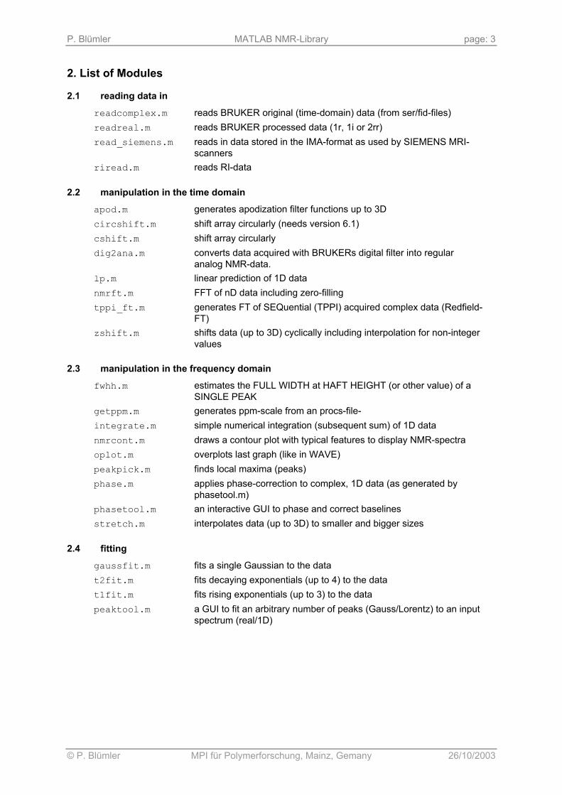
2. List of Modules 2.1 reading data in

readcomplex.m reads BRUKER original (time-domain) data (from ser/fid-files) readreal.m reads BRUKER processed data (1r, 1i or 2rr) read_siemens.m reads in data stored in the IMA-format as used by SIEMENS MRI-

scanners riread.m reads RI-data

2.2 manipulation in the time domain

apod.m generates apodization filter functions up to 3D circshift.m shift array circularly (needs version 6.1) cshift.m shift array circularly dig2ana.m converts data acquired with BRUKERs digital filter into regular

analog NMR-data. lp.m linear prediction of 1D data nmrft.m FFT of nD data including zero-filling tppi_ft.m generates FT of SEQuential (TPPI) acquired complex data (Redfield-

FT) zshift.m shifts data (up to 3D) cyclically including interpolation for non-integer

values 2.3 manipulation in the frequency domain

fwhh.m estimates the FULL WIDTH at HAFT HEIGHT (or other value) of a SINGLE PEAK

getppm.m generates ppm-scale from an procs-file- integrate.m simple numerical integration (subsequent sum) of 1D data nmrcont.m draws a contour plot with typical features to display NMR-spectra oplot.m overplots last graph (like in WAVE) peakpick.m finds local maxima (peaks) phase.m applies phase-correction to complex, 1D data (as generated by

phasetool.m) phasetool.m an interactive GUI to phase and correct baselines stretch.m interpolates data (up to 3D) to smaller and bigger sizes

2.4 fitting

gaussfit.m fits a single Gaussian to the data t2fit.m fits decaying exponentials (up to 4) to the data t1fit.m fits rising exponentials (up to 3) to the data peaktool.m a GUI to fit an arbitrary number of peaks (Gauss/Lorentz) to an input

spectrum (real/1D)



2.5 general

dimension.m calculates the dimensionality of the data ellips.m displays tensors as ellipsoids. getdrives.m gets the drive letters of all mounted filesystems on the computer gmax.m global maximum of a data-set with arbitrarily many dimensions gmin.m global minimum of a data-set with arbitrarily many dimensions plotline.m plots horizontal or vertical line rot_xyz.m returns the rotation matrix for successive rotation by an angle around

the x-axis, another around the y-axis and a last around the z-axis. subdirs.m returns the subdirectories of a directory ufo.m displays tensors in a special 'UFO' way (largest eigen value = spike,

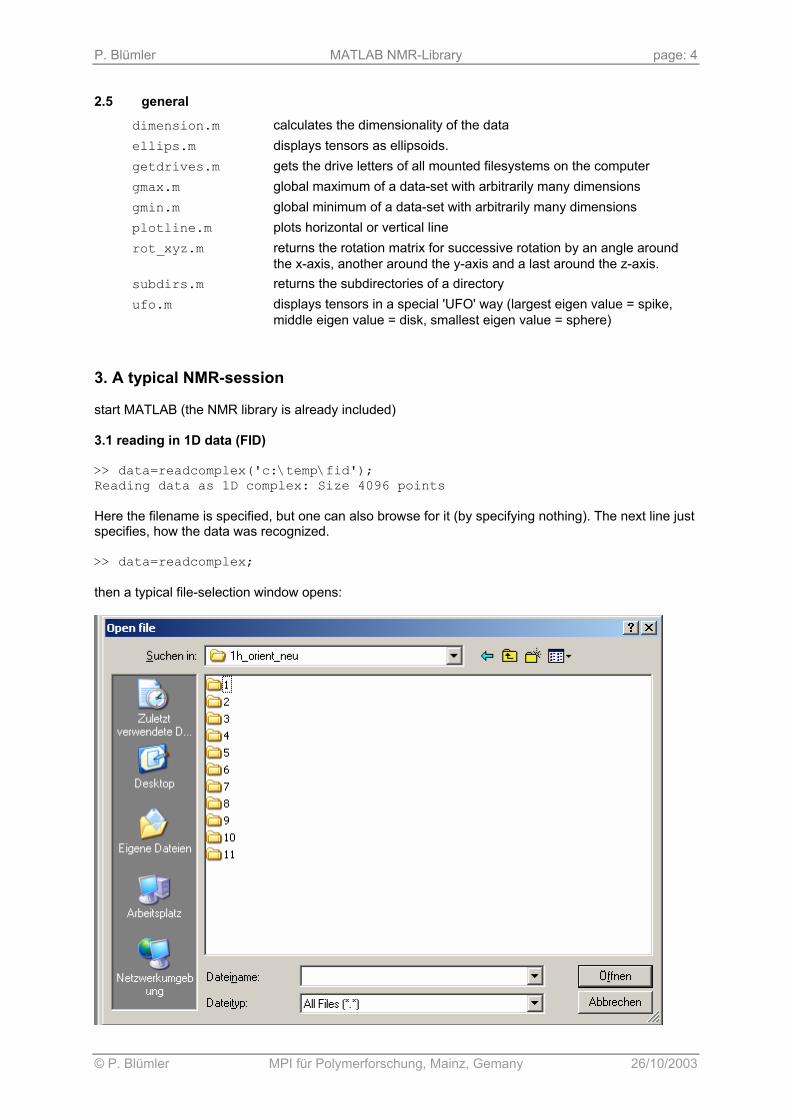
middle eigen value = disk, smallest eigen value = sphere) 3. A typical NMR-session start MATLAB (the NMR library is already included) 3.1 reading in 1D data (FID) >> data=readcomplex('c:\temp\fid'); Reading data as 1D complex: Size 4096 points Here the filename is specified, but one can also browse for it (by specifying nothing). The next line just specifies, how the data was recognized. >> data=readcomplex; then a typical file-selection window opens:



Once the data is read in, one might want to have a glance on it, by simply typing >> plot(data) gives a complex-plot (real vs. imag part).

If one wants to look at the real part only, type >> plot(real(data))



or just plotting the first 128 points of both real and imaginary part: >> plot(real(data(1:128)),'k') >> oplot(imag(data(1:128)),'r')

One clearly sees that the first ca. 50 points look weird due to BRUKERs digital filter. One has to remove them before continuing, or FT-data will look as weird, >> data=dig2ana(data); >> plot(real(data(1:128)),'k') >> oplot(imag(data(1:128)),'r') better!

range color



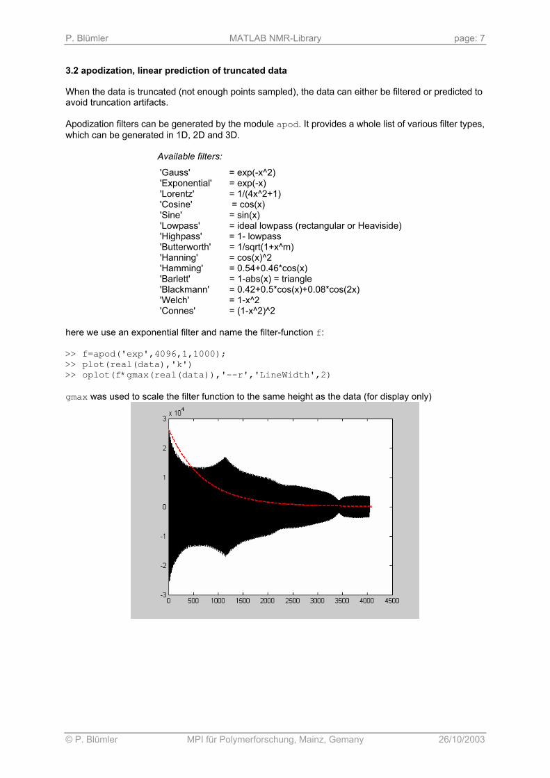
3.2 apodization, linear prediction of truncated data When the data is truncated (not enough points sampled), the data can either be filtered or predicted to avoid truncation artifacts. Apodization filters can be generated by the module apod. It provides a whole list of various filter types, which can be generated in 1D, 2D and 3D.

Available filters:

'Gauss' = exp(-x^2) 'Exponential' = exp(-x) 'Lorentz' = 1/(4x^2+1) 'Cosine' = cos(x) 'Sine' = sin(x) 'Lowpass' = ideal lowpass (rectangular or Heaviside) 'Highpass' = 1- lowpass 'Butterworth' = 1/sqrt(1+x^m) 'Hanning' = cos(x)^2 'Hamming' = 0.54+0.46*cos(x) 'Barlett' = 1-abs(x) = triangle 'Blackmann' = 0.42+0.5*cos(x)+0.08*cos(2x) 'Welch' = 1-x^2 'Connes' = (1-x^2)^2

here we use an exponential filter and name the filter-function f: >> f=apod('exp',4096,1,1000); >> plot(real(data),'k') >> oplot(f*gmax(real(data)),'--r','LineWidth',2) gmax was used to scale the filter function to the same height as the data (for display only)



Now we multiply the data with the filter-function. But before, we save the original data into another variable (odata): >> odata=data; >> data=odata.*f; >> plot(real(data),'k')

Linear prediction tries to estimate the data into the future (or past). Do not overdo it, process is quite time consuming! This example tries to predict 1000 points based on the last 200 points of the original data: >> data=lp(odata,1000,200); >> plot(real(data))



3.3 Zero-filling and Fourier-transformation Zero-filling can be done by hand by first generating a bigger vector of zeros and then inserting the data: >> new_data=zeros(16384,1); >> s=size(odata) s = 4096 1 >> new_data(1:s)=odata; >> plot(real(new_data));

The routine nmrft does the FFT with the correct shifts (to avoid phasing problems). The second argument is the resulting size after the FT. If this number is bigger than the original data-size, zero-filling is applied (be careful to avoid truncation artifacts), if it is smaller the data is truncated itself. In the following example the data is to be blown up to 16384 data points (without and with filtering). >> s=nmrft(odata,2^14); >> plot(abs(s(6000:7200))) now with the filter-function >> s=nmrft(odata.*f,2^14); >> plot(abs(s(6000:7200)),'r')



3.4 Phasing the data (frequency domain) >> spec=nmrft(readcomplex,256); this is just for demo of concatenation of MATLAB commands, and to switch to a more realistic data-set >> plot(real(spec),'k'); >> oplot(imag(spec),'r');

we see the data is not phased correctly (lousy experimenter!). To determine the best phasing parameters we call a GUI (graphical user interface) called phasetool. To explain what it does we look into the help-header: >> help phasetool ############################################################################ # # function PHASETOOL # # generates an interactive GUI to phase data # data must be complex, Fourier-transformed and one-dimensional! # # PH0 is zeroth order phase correction in degrees # PH1 is first order phase correction in degrees/(number of points in the input . # data)*1000 # pivot is the origin for PH1 in points # # usage: phasetool(data,pval,base); # # INPUT (calling): # data = input data (1D, complex) # pval = OPTIONAL predefined phase values (3x1 vector) # [p1,p2,p3] with p1 = PH0 value in degrees # p2 = PH1 value in degrees/number of data points*1000 # p3 = pivot in points # base = OPTIONAL baseline (vector of length of data) # # OUTPUT (returning) # when the function is called with pval, it contains the phase values (3x1 vector) # after returning. Recursive calls will therefore reuse the last values!!!! # If not specified (calling "phasetool(data)" only) will notify that the phase values # can be found in the working place in the variable "phase_values". # The same works with/without base (if not specified the values are returned in the # variable "baseline". # # (c) P. Blümler 1/03 ############################################################################ ---------------------------------------------------------------------------- version 1.2 PB 6/2/03 (please change this when code is altered) added fixed colors for UNIX



Let’s call it without predefined phase values: >> phasetool(spec) After exiting the results will automatically be stored in the variables: "phase_values" and "baseline" (latter if accessed) the GUI-window will pop up:

by using the sliders one eventually is satisfied with the result. By pressing the EXIT-button one returns to the MATLAB command-line mode. The chosen phase-values are (if one didn’t specify them explicitly, see help above) in a variable named phase_values >> phase_values phase_values = -65.3400 -20.9849 195.0000 The spectrum still is not altered and one has to apply these values in a separate routine called phase. This is because one might want to apply these values repetitively to 2D-data, for instance. >> spec=phase(spec,phase_values); >> plot(real(spec),'k'); >> oplot(imag(spec),'r'); hurray!

automatically determined pivot

0th order phase correction

1st order phase correction

manual pivot selection

values

sensitivity

range

controls for appearance of the spectrum



3.5 Integration and peak picking

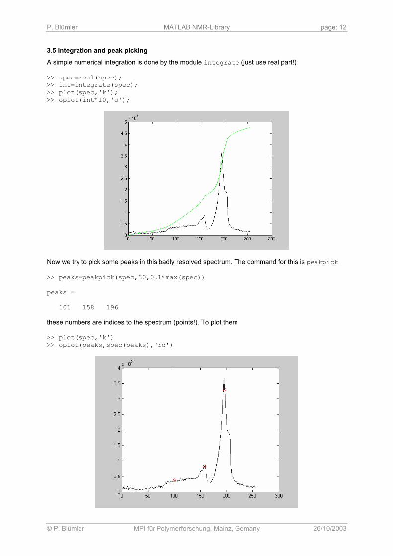
A simple numerical integration is done by the module integrate (just use real part!) >> spec=real(spec); >> int=integrate(spec); >> plot(spec,'k'); >> oplot(int*10,'g');

Now we try to pick some peaks in this badly resolved spectrum. The command for this is peakpick >> peaks=peakpick(spec,30,0.1*max(spec)) peaks = 101 158 196 these numbers are indices to the spectrum (points!). To plot them >> plot(spec,'k') >> oplot(peaks,spec(peaks),'ro')



3.6 Displaying and exporting the result

One can control all plotting commands from the command line mode, but this needs a lot of explaining. One best examines the MATLAB help text for the following commands: >> ppm=getppm('c:\temp\procs'); % gets the ppm-scale from the proc file >> plot(ppm,spec,'k','LineWidth',2); >> oplot(ppm(peaks),spec(peaks),'rs','LineWidth',2,... 'MarkerEdgeColor','k', 'MarkerFaceColor','g','MarkerSize',10); >> oplot(ppm,int*8,'--r'); >> set(gca,'XDir','Reverse') % reverses the x-axis (ppm!) >> set(gca,'YColor','w','YTickLabel',''); % switches y-axis off >> set(gca,'Box','off'); % switches upper axis off >> xlabel('^{1}H frequency [ppm]'); %x-axis annotation >> legend('spectrum','reference peaks','integral',2) %plot legend >> % add some title >> text(11,2.5e5,'sample 1: spectrum \cdot exp(-\it{i}\pi)',... 'FontSize',14,'Color',[.1,.2,0.8]) >> set(gcf,'Color','w'); %set figure background to white this then looks like that



…or one can also use the menu of the plot window….

This can then be exported either by copying to the clipboard (Edit|Copy Figure) or by (File|Export) to some compatible file-format (EPS, TIF, JPG, BMP…etc.) 3.7 2D/nD-data

Reading in nD data is the same as for 1D, but one has to specify the size of n-1 dimensions, so that readcomplex can guess the remaining by the file size. Alternatively one can use the browser and the command reshape: >> data=readcomplex('C:\temp\ser',128); Reading data as 2D complex: Size 128 x 1024 points >> data=readcomplex('C:\temp\ser',128,128); Reading data as 3D complex: Size 128 x 128 x 8 points >> data=readcomplex; Reading data as 1D complex: Size 131072 points >> data=reshape(data,256,32,16); All the other procedures are principally the same, e.g. >> data=readcomplex; Reading data as 1D complex: Size 16384 points >> data=reshape(data,128,128); >> f=apod('G',[128,128],[64,64],[50,40]); %creating 2D filter-function >> data=nmrft(data.*f,256,256); %2D FT incl. zero-filling



However some (like phase, phasetool etc.) only work on 1D data. So one has to specify a certain slice from the 2D data-set >> phasetool(data(:,64)); After exiting the results will automatically be stored in the variables: "phase_values" and "baseline" (latter if accessed) and then apply this representative phase to all slices for rows >> for k=1:256, data(k,:)=phase(data(k,:),phase_values); end for columns (note the transpose!) >> for k=1:256, data(:,k)=phase(data(:,k),phase_values)'; end By this one can apply all 1D commands to nD data. The main difference is the visualization. Therefore, some examples are presented in the following. They can be edited like 1D plots, but –of course– have some special keywords. Refer to MATLABs help desk for more information. The standard way of presenting 2D-NMR data is the contour-plot. MATLABs build-in command contour has been slightly modified in the module nmrcont to meet the needs of NMR-people. >> nmrcont(data); %left graph: default 10 contours >> nmrcont(data,[0.5:.5:gmax(data)]); >> %right graph: specifying contours from 0.5 to max in steps of 0.5

Next also axes are introduced and the linewidth is increased to 2. >> x=linspace(-1,1,256); >> y=linspace(-2,3,256); >> c=linspace(0.5,gmax(data),17); >> nmrcont(data,x,y,c,2);



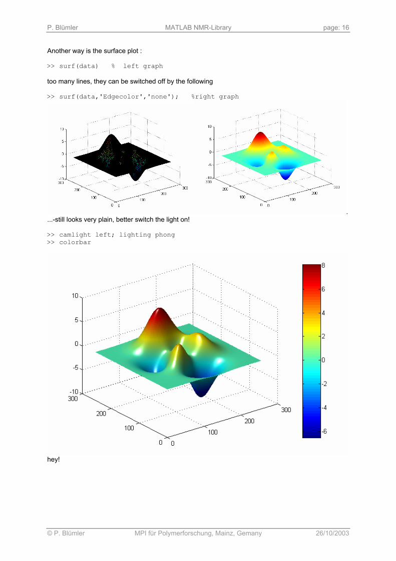
Another way is the surface plot : >> surf(data) % left graph too many lines, they can be switched off by the following >> surf(data,'Edgecolor','none'); %right graph

....-still looks very plain, better switch the light on! >> camlight left; lighting phong >> colorbar

hey!



Another way of displaying data is the so-called waterfall: >> h=waterfall(s); >> view(-10,45); %change the orientation >> set(h,'Edgecolor','k'); %set line color to black

Some people prefer images, so there is also a routine for that: >> imagesc(data) >> axis equal; axis off % left image >> imagesc(data,[1e5,7e5]); >> % specifying the color range, lower = black, higher = white (or whatever >> % this corresponds to for the actual colormap >> axis equal; axis off >> colormap gray %middle image >> colorbar; >> colormap cool; %right image



3.8 Fitting Curves to Data

For simple equations MATLAB provides a basic fitting tool in each 1D-plot (Tool|Basic Fitting). Here is an example for a linear fit: >> x=linspace(0,10,100); >> y=10.3-3.12*x+randn(1,100); >> plot(x,y,'o')

and the result



Fitting Gaussians with gaussfit:

The module gaussfit performs a single Gaussian fit to the data. It needs no guessing values, but rather does some semi-intelligent guesses itself. One can specify what should be varied by selecting the third input variable, n, as follows (the fourth controls if a plot should be done):

n = control on fit parameters (optional, default=4) n = 2 : only width and amplitude are fitted n = 3 : width, ampl. and origin are fitted n = 4 : all fitted n = 5 : width, ampl. and offset fitted

for example: >> p=[10.23,5.44,0.123,2.344]; >> x=linspace(-1,1,30); >> y=p(1)*exp(-(x-p(3)).^2*p(2))+p(4)+.4*randn(1,30); >> n=4; >> [ip,delta]=gaussfit(x,y,n,1) ip = 9.8609 5.8730 0.1305 2.7176 delta = 0.4140 0.6835 0.0123 0.2864 the ip-values are the fitted parameters (amplitude, width, origin, offset) and their errors are estimated by delta. The plot looks like that (green lines are some idea of the confidence interval).



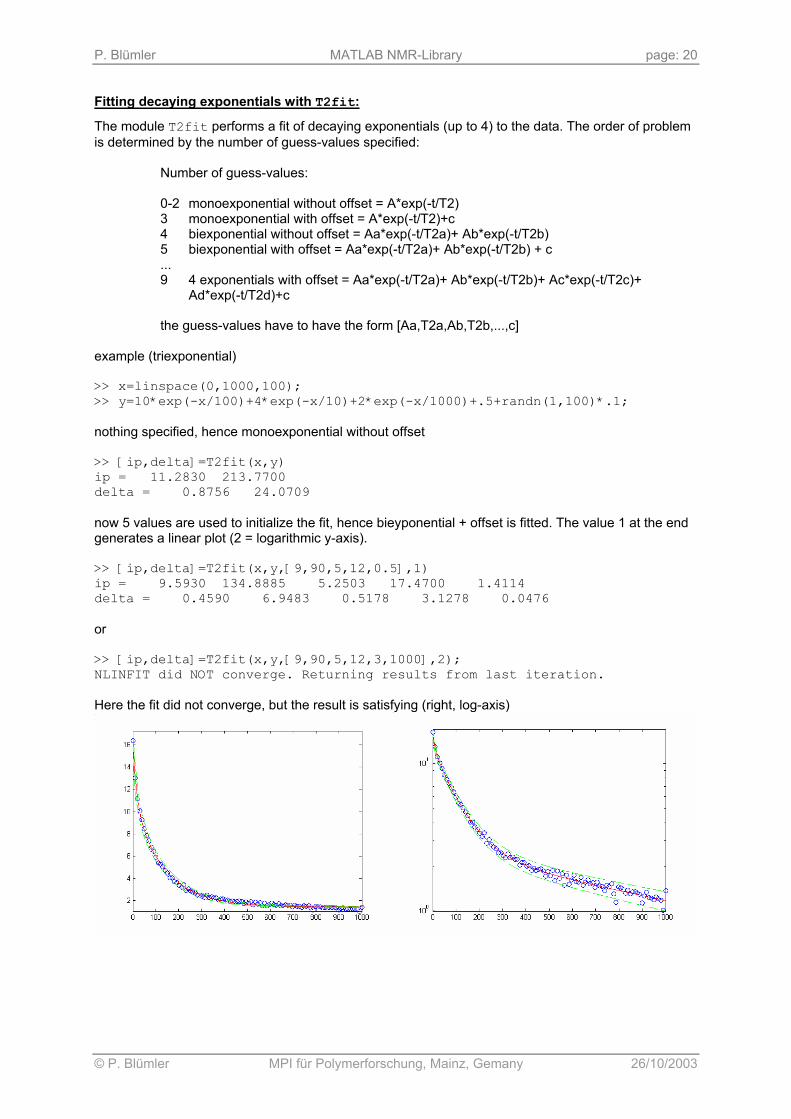
Fitting decaying exponentials with T2fit:

The module T2fit performs a fit of decaying exponentials (up to 4) to the data. The order of problem is determined by the number of guess-values specified:

Number of guess-values: 0-2 monoexponential without offset = A*exp(-t/T2) 3 monoexponential with offset = A*exp(-t/T2)+c 4 biexponential without offset = Aa*exp(-t/T2a)+ Ab*exp(-t/T2b) 5 biexponential with offset = Aa*exp(-t/T2a)+ Ab*exp(-t/T2b) + c ... 9 4 exponentials with offset = Aa*exp(-t/T2a)+ Ab*exp(-t/T2b)+ Ac*exp(-t/T2c)+

Ad*exp(-t/T2d)+c the guess-values have to have the form [Aa,T2a,Ab,T2b,...,c]

example (triexponential) >> x=linspace(0,1000,100); >> y=10*exp(-x/100)+4*exp(-x/10)+2*exp(-x/1000)+.5+randn(1,100)*.1; nothing specified, hence monoexponential without offset >> [ip,delta]=T2fit(x,y) ip = 11.2830 213.7700 delta = 0.8756 24.0709 now 5 values are used to initialize the fit, hence bieyponential + offset is fitted. The value 1 at the end generates a linear plot (2 = logarithmic y-axis). >> [ip,delta]=T2fit(x,y,[9,90,5,12,0.5],1) ip = 9.5930 134.8885 5.2503 17.4700 1.4114 delta = 0.4590 6.9483 0.5178 3.1278 0.0476 or >> [ip,delta]=T2fit(x,y,[9,90,5,12,3,1000],2); NLINFIT did NOT converge. Returning results from last iteration. Here the fit did not converge, but the result is satisfying (right, log-axis)



Fitting rising exponentials with T1fit:

The module T1fit performs a fit of rising exponentials (up to 3) to the data. It does that in a physical way. Any T1 recovery-data (saturation or inversion recovery) is described by:

( )

−−−= ∞∞

1exp)0()(

TtMMMtM zzzz

where zM∞ is the z-magnetization at infinite time and )0(zM at the beginning of the sequence (ideally

for inversion- zz MM ∞−=)0( and 0)0( =zM for saturation-recovery). For a system on n components (fraction xi) this equation can be rewritten as:

∑∑==

∞

−+

−−=

n

ii

in

ii

iz

TtM

TtMtM

1 11 1

exp)0(exp1)(

Like in T2fit the order of the fit is determined by the number of guess-values specified:

Number of guess-values: 0-3 monoexponential = A-(A-B)*exp(-t/T1) 6 biexponential = Aa-(Aa-Ba)*exp(-t/T1a)+ Ab-(Ab-Bb)*exp(-t/T1b) 9 triiexponential = Aa-(Aa-Ba)*exp(-t/T1a)+ Ab-(Ab-Bb)*exp(-t/T1b)+ )+ Ac-(Ac-

Bc)*exp(-t/T1c) the guess-values have to have the form [Aa,Ba,T1a,Ab,BbT1b,...] with A = zM∞ , B = )0(zM

>> x=linspace(0,1000,100); >> y=10*(1-exp(-x/100))+randn(1,100)*.1; %saturation recovery >> T1fit(x,y) ans = 9.9909 -0.0035 100.2743 >> T1fit(x,y,[10,1,90],1) %make a plot ans = 9.9909 -0.0035 100.2743 >> y=10*(1-1.9*exp(-x/100))+5*(1-1.9*exp(-x/30))+randn(1,100)*.1; >> T1fit(x,y,[20,2,90,10,2,10],1) ans = 13.1792 -7.4436 94.8264 1.8006 -6.0649 25.2145



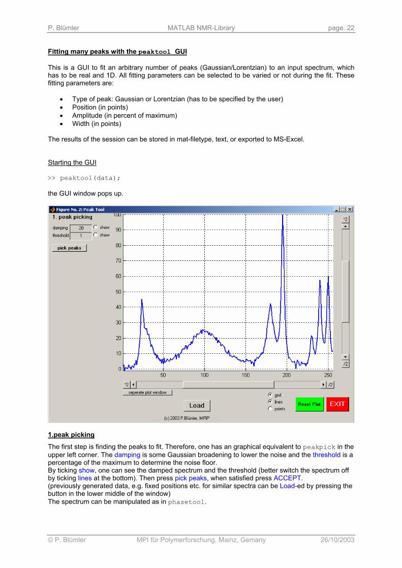
Fitting many peaks with the peaktool GUI This is a GUI to fit an arbitrary number of peaks (Gaussian/Lorentzian) to an input spectrum, which has to be real and 1D. All fitting parameters can be selected to be varied or not during the fit. These fitting parameters are:

• Type of peak: Gaussian or Lorentzian (has to be specified by the user) • Position (in points) • Amplitude (in percent of maximum) • Width (in points)

The results of the session can be stored in mat-filetype, text, or exported to MS-Excel. Starting the GUI >> peaktool(data); the GUI window pops up.

1.peak picking

The first step is finding the peaks to fit. Therefore, one has an graphical equivalent to peakpick in the upper left corner. The damping is some Gaussian broadening to lower the noise and the threshold is a percentage of the maximum to determine the noise floor. By ticking show, one can see the damped spectrum and the threshold (better switch the spectrum off by ticking lines at the bottom). Then press pick peaks, when satisfied press ACCEPT. (previously generated data, e.g. fixed positions etc. for similar spectra can be Load-ed by pressing the button in the lower middle of the window) The spectrum can be manipulated as in phasetool.



This looks good (missing peaks, can be inserted later), so ACCEPT is pressed and the GUI changes to the fitting view. 2. peak fitting

The fitting part looks like this (you can go back by pressing <UNDO)

peaks: type and area

change type of selected peak

selected peak

fitting parameters



Peaktool starts with a first guess of the spectrum, which is displayed by an overlaid fit-spectrum (thin black line = sum of peaks, one can change/add this by ticking individual peaks = red, or residuals = green at the bottom of the window) The next step is to insert a new peak by pressing Insert Peak (left). Then the color of the button changes to yellow and DONE!. The cursor becomes a crosshair and you can click anywhere in the spectrum to insert new peaks (by default Gaussian). When done, press DONE! (It might take two clicks to register, please be patient!!!) Now the peaks are changed to what one thinks that they represent (Lorentzian or Gaussian). By selecting them from the list in the upper left corner (the marker in the spectrum will change to yellow to indicate the selected peak) and alter them by pressing Gauss -> Lorentz button or vice versa. When satisfied the fitting can start: It is good advice to change the fitting parameters one after another until the fit is stable to optimize all at once. This clearly also depends on the quality and kind of spectrum. Each fitting step has to be prepared by telling the program which parameters one wants to vary. If the vary field is ticked, this parameter is varied for the selected peak. Of course one can select as many as one likes (loosing stability of the fit). One can also simply set one or more parameters to vary for all peaks during the fit by ticking the all field (logically changing to none). The color of each marker will change from dark to medium to light red, indicating how many parameters are selected for each peak (dark red = 1, medium = 2, light = all). One can –of course– also vary the parameters manually, simply be typing in the according box. As soon as parameters are determined to vary a new section of the window appears, showing the fitting parameters (parameter tolerance, residual tolerance and maximum number of iterations), which can be altered to stabilize or speed up the fitting process. Finally also the FIT! button appears in green. As soon as you press it the fitting starts.

one selected

two selected

all selected



The color of the FIT! Button also indicates if the fit was stable (changing to red means that you want too much!) Another good advice is to follow this recipe:

1. ONLY varying the amplitude 2. ONLY varying the width 3. varying width AND amplitude 4. vary everything

3. Exporting results:

at certain times one should save the results, because there is NO UNDO during the fitting process!! Loading works alike. One can also export the graphics to a separate plot window, where annotations, export to BMP etc. can be performed.

Finally, the results can be exported to an Excel spreadsheet using the >Excel button.



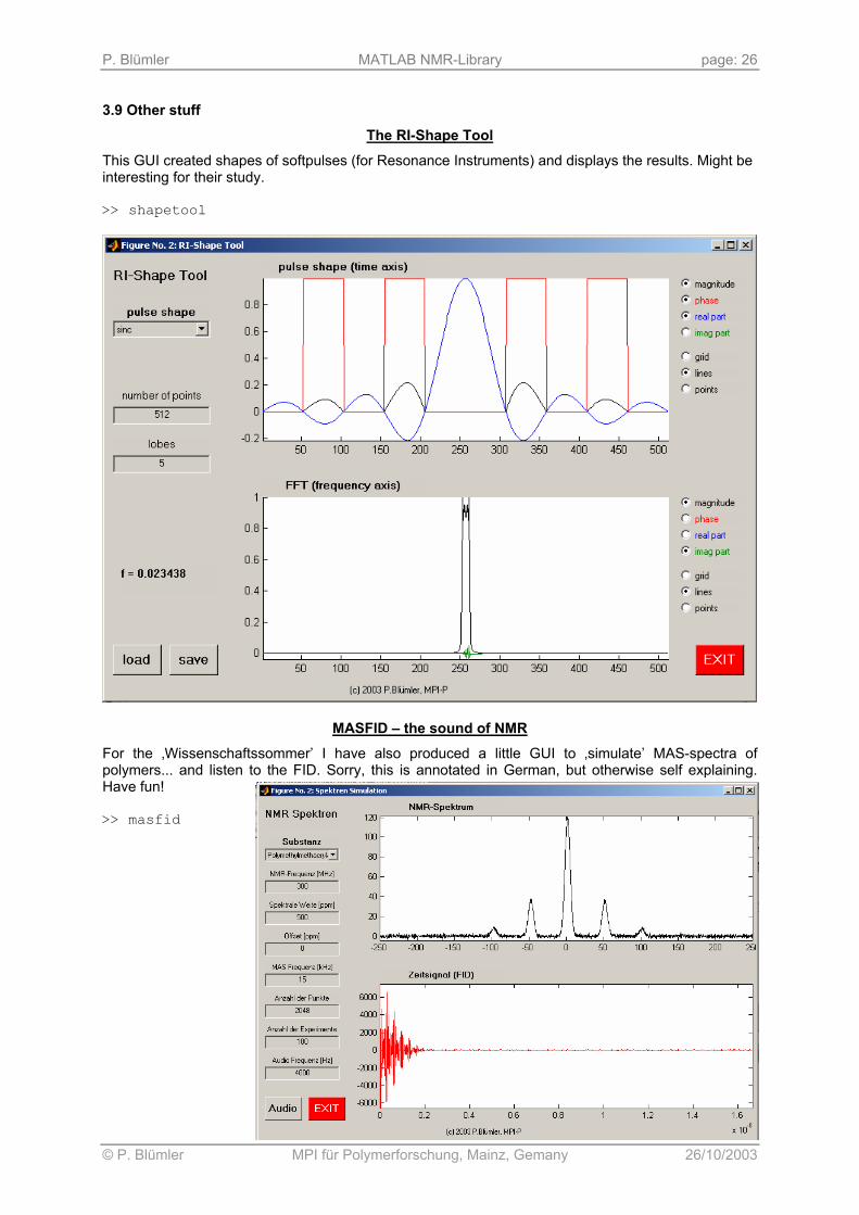
3.9 Other stuff

The RI-Shape Tool

This GUI created shapes of softpulses (for Resonance Instruments) and displays the results. Might be interesting for their study. >> shapetool

MASFID – the sound of NMR

For the ‚Wissenschaftssommer’ I have also produced a little GUI to ‚simulate’ MAS-spectra of polymers... and listen to the FID. Sorry, this is annotated in German, but otherwise self explaining. Have fun! >> masfid



4. Alphabetical listing of help text to the modules

APOD.M (author: PB) generates apodization filter functions up to 3D usage: ffunc=apod(type,size,center,width,mode) type = filter functional (see below) size = length of dimensions, also handels dimensionality in points center = center of filter functions (0 for FID, size/2 for echos) in points* width = width of filter in points (typically full width at half height)* mode = steepness of filter function (exponent of argument)* * = optional (defaults: center = size/2, width=size/4; mode = 1); 1D-example: >>plot(apod('gauss',256,128,100)); 2D-example: >>surf(apod('blackmann',[256,256],[128,128],[100,70]),.. 'Edgecolor','none');camlight left Filter functionals (types): is not case-sensitive (abbrevaitions are allowed (see case at end) 'Gauss' = exp(-x^2) 'Exponential' = exp(-x) 'Lorentz' = 1/(4x^2+1) 'Cosine' = cos(x) 'Sine' = sin(x) 'Lowpass' = ideal lowpass (rectangular or Heaviside) 'Highpass' = 1- lowpass 'Butterworth' = 1/sqrt(1+x^m) 'Hanning' = cos(x)^2 'Hamming' = 0.54+0.46*cos(x) 'Barlett' = 1-abs(x) = triangle 'Blackmann' = 0.42+0.5*cos(x)+0.08*cos(2x) 'Welch' = 1-x^2 'Connes' = (1-x^2)^2

CIRCSHIFT.M (author: MATLAB)

CIRCSHIFT Shift array circularly. B = CIRCSHIFT(A,SHIFTSIZE) circularly shifts the values in the array A by SHIFTSIZE elements. SHIFTSIZE is a vector of integer scalars where the N-th element specifies the shift amount for the N-th dimension of array A. If an element in SHIFTSIZE is positive, the values of A are shifted down (or to the right). If it is negative, the values of A are shifted up (or to the left). Examples: A = [ 1 2 3;4 5 6; 7 8 9]; B = circshift(A,1) % circularly shifts first dimension values down by 1. B = 7 8 9 1 2 3 4 5 6 B = circshift(A,[1 -1]) % circularly shifts first dimension values % down by 1 and second dimension left by 1. B = 8 9 7 2 3 1 5 6 4 See also FFTSHIFT, SHIFTDIM.

CSHIFT.M (author: PB) shifts data (up to 4D) cyclically, shifts can be positive or negative or zero. If a shift range is not specified, the routine applies the shifts to the first dimension(s) and assumes zero shift for the others. usage: shdata=cshift(data,s1,s2,...);



DIG2ANA.M (author: RG) converts data acquired with BRUKERs digital filter into regular analog NMR-data. This is a preliminary version of the routine which needs some information from the acqus file, and therefore will work only if you are in the datafolder of spectrometers or you have copied the acqus file together with the data (which is not a bad idea in any case). usage: data_ana=dig2ana(data_dig);

DIMENSION.M (author: PB) calculates the dimensionality of the data (not like ndims) usage: dim=dimension(data); result: dim==0 data is scalar dim==1 data is 1D vector dim==2 data is 2D dim>2 data is nD (n>2)

ELLIPS.M (author: PB) displays tensors as ellipsoids. The color is chosen by the average eigen value on the actual colormap. usage ellips(n,d,v,dmax,xoffset,yoffset) n = point resolution of graphics d = (3x1) vector of the eigen values v = (3x3) matrix of the eigen vectors dmax = maximum eigen value xoffset = offset of x-axis of plot for continous display yoffset = offset of y-axis of plot for continous display

FWHH.M (author: PB) Estimates the FULL WIDTH at HAFT HEIGHT (or value) of a SINGLE PEAK specified by input! The algorithm looks for the next neighbouring points where the input data is less the value of the data at the specified point and takes the average (if possible). usage: width=fwhh(data,point,value); data = data to analyze point = specifies the point to analyze value = optional (default = 0.5) specify if not half (=0.5) height

GAUSSFIT.M (author: PB)

fits a Gaussian with variable parameter number to data. The general Gauss-model is : f(x)= amplitude*exp(-(x-origin).^2*width)+offset call: par = gaussfit(x,y); [par,delta]=gaussfit(x,y); [par,delta]=gaussfit(x,y,n); [par,delta]=gaussfit(x,y,n,out); par = fitted parameter [amplitude, width, origin, offset] delta = error estimate (optional) in abs. values n = control on fit parameters (optional, default=4) n = 2 : only width and amplitude are fitted n = 3 : width, ampl. and origin are fitted n = 4 : all fitted n = 5 : width, ampl. and offset fitted out = creates output plot for being different from 0 (optional, default =0)



EXAMPLE: >> n=11; >> p=[10.23,5.44,0.123,2.344]; >> x=linspace(-1,1,n); >> y=p(1)*exp(-(x-p(3)).^2*p(2))+p(4)+.4*randn(1,n); >> [ip,delta]=gaussfit(x,y,4,1)

GETDRIVES.M (author: MATLAB)

GETDRIVES Get the drive letters of all mounted filesystems on the computer. F = GETDRIVES returns the roots of all mounted filesystems on the computer as a cell array of char arrays. For UNIX this list consists solely of the root directory, /. For Microsoft Windows, it is a list of the names of all one-letter mounted drive letters. F = GETDRIVES('-nofloppy') does not scan for the a: or b: drives on Windows, which usually results in annoying grinding sounds coming from the floppy drive. F = GETDRIVES('-twoletter') scans for both one- AND two-letter drive names on Windows. While two-letter drive names are technically supported, their presence is in fact rare, and slows the search considerably. Note that only the names of MOUNTED volumes are returned. In particular, removable media drives that do not have the media inserted (such as an empty CD-ROM drive) are not returned. See also EXIST, COMPUTER, UIGETFILE, UIPUTFILE. Copyright 2001 Bob Gilmore. Email bug reports and comments to [email protected]

GETPPM.M (author: PB) generates a ppm-scale from a BRUKER procs-file usage: ppm=getppm('procs');

GMAX.M (author: MATLAB)

GMAX Global maximum. Y = GMAX(X) return the global maximum value of X. [Y,POS] = GMAX(X) returns the value and position of the global maximum. If X has more than one global maximum only the position of the first will be returned.

GMIN.M (author: MATLAB)

GMIN Global minimum. y = GMIN(X) return the global maximum value of X . [Y,POS] = GMIN(X) returns the value and position of the global minimum. If X has more than one global minimum only the position of the first will be returned.

INTEGRATE.M (author: PB) simple numerical integration (subsequent sum) of 1D data usage: int=integrate(data);



LP.M (author: PB) linear prediction of 1D data (can be complex!) usage: lpdata=lp(data,nfut,npoles); data = data to predict nfut = number of points to predict (>0 = future, <0 = past) npoles = number of reference points in the data (>= number of data points - 1). Strongly influences result!

NMRCONT.M (author: PB) draws a contour plot with typical features to display NMR-spectra. no annotations, all black,axes specified by 1D vectors usage: nmrcont(data,v); low level application data=2D real data array v=1D [OPTIONAL] vector specifying the contour levels if submitted as a single number, v levels are drawn from min to max, default = 10 usage: nmrcont(data,x,y,v,thick); data=2D real data array x=1D vector specifying the range of the x-axis y=1D vector specifying the range of the y-axis v=1D vector specifying the contour levels if submitted as a single number, v levels are drawn from min to max thick=[optional] sets the linewidth, default=1

NMRFT.M (author: PB) does the NMR specific FFT on nD-data (icluding zero-filling and shift of zero-frequency to center). For correct phase, the data has to start at the left (FID type)...point 1 = time 0. The optional dimension parameter controls the size after the FT. If chosen bigger than the original, zero-filling is applied, if not specified the size is kept the same, if smaller the data is truncated. usage: ftdata=nmrft(data,dims); data = data to do the FFT on dims = [OPTIONAL] resulting size after (if bigger than original, zero-filling is applied)

OPLOT.M (author: PB) adaption of WAVE command OPLOT. Simply overplots previous plot. usage: oplot(x,y,'...');

PEAKPICK.M (author: PB) finds local maxima (peaks) usage: peaks=peakpick(data,fw,offset,plot); data = input spectrum (1D, real) peaks = output index of peak found fw = OPTIONAL, smoothing strength, default=20 offset = OPTIONAL, noise offset (green line in plot) plot = OPTIONAL, if not 0 plot is generated example: pp=peakpick(data,500,0.01*max(data),1); data(pp)



PHASE.M (author: PB) applies phase-correction to complex, 1D data usage: pdata=dimension(data,phase); or: pdata=dimension(data,[-1.23,0.001,123]); phase = values for phase-correction (see phasetool.m for details) dim==1 data is 1D vector dim==2 data is 2D dim>2 data is nD (n>2)

PHASETOOL.M (author: PB) generates an interactive GUI to phase data data must be complex, Fourier-transformed and one-dimensional! PH0 is zeroth order phase correction in degrees PH1 is first order phase correction in degrees/(number of points in the input data)*1000 pivot is the origin for PH1 in points usage: phasetool(data,pval,base); INPUT (calling): data = input data (1D, complex) pval = OPTIONAL predefined phase values (3x1 vector) [p1,p2,p3] with p1 = PH0 value in degrees p2 = PH1 value in degrees/number of data points*1000 p3 = pivot in points base = OPTIONAL baseline (vector of length of data) OUTPUT (returning) when the function is called with pval, it contains the phase values (3x1 vector) after returning. Recursive calls will therefore reuse the last values!!!! If not specified (calling "phasetool(data)" only) will notify that the phase values can be found in the working place in the variable "phase_values". The same works with/without base (if not specified the values are returned in the variable "baseline".

PLOTLINE.M (author: MATLAB)

PLOTLINE Plots a vertical or horizontal line PLOTLINE(x,dir) plots a horizontal (dir='h') or vertical (dir='v') dotted line at position x on the current figure. PLOTLINE(x,dir,S) uses plots the line using the specified color and linestyle. S is a string containing one element from any or all the columns bellow (just like in the plot command). Colors: Styles: y yellow - solid m magenta : dotted c cyan -. dashdot r red -- dashed g green b blue w white k black PLOTLINE(...,'label') plots the value label x next to the line.

READ_SIEMENS.M (author: PB) reads in data stored in the IMA-format as used by SIEMENS MRI-Scanners usage: data=read_siemens(filename);



READCOMPLEX.M (author: PB) reads in data as max. 4D complex arrays from typical BRUKER SER or FID files. If dimensions (n(1)...n(4)) are specified, the routine generates according dimensions. If the product of dimensions is smaller than the data length, the routine tries to estimate/generate the next higher dimension. Hence, if nothing but the filename is specified the data are read in as 1D. usage: data=readcomplex(filename,n(1),n(2),...); filename = optional, browser opens if nothing is specified n(1)...n(4) = optional dimensions (estimated from data length if not present)

READREAL.M (author: PB) reads in data as max. 4D real arrays from typical BRUKER process files. If dimensions (n1...n4) are specified, the routine generates according dimensions. If the product of dimensions is smaller than the data length, the routine tries to estimate/generate the next higher dimension. Hence, if nothing but the filename is specified the data are read in as 1D. usage: data=readreal(filename,n1,n2,...); n1...n4 = optional dimensions (estimated from data length if not present)

ROT_XYZ.M (author: PB) returns the rotation matrix for successive rotation by an angle a around the x-axis, b around the y-axis and c around the z-axis. a,b,c have to be in RADIANS. Rx(a)Ry(b)Rz(c) usage R=rot_xyz(a,b,c); R = resulting rotation matrix a = rotation angle around x-axis in radians b = rotation angle around y-axis in radians c = rotation angle around z-axis in radians

SHAPETOOL.M (author: PB) GUI to calculate and diplay different RF-shapes (soft pulses) and their FT (linear response!). The save-format is adapted to RI-spectrometers. The f-value shows the effective bandwidth (full width at half hight) relative to the entire region (no. points). usage: shapetool

STRETCH.M (author: PB) interpolates data (up to 3D) to smaller and bigger sizes. usage: intdata=stretch(data,dims,method); data = data to interpolate dims = vector with new dimensions (missing dimensions are set to that of the original -- no interpolation) method = OPTIONAL see interp1-3 help files (default is linear)

SUBDIRS.M (author: MATLAB) SUBDIRS Returns the subdirectories of a directory Y = SUBDIRS(X) returns a cell array containing the names of the first level subdirectories of directory 'x'. Y = SUBDIRS(X,L) does the same untill subdirs level L. Y = SUBDIRS(X,'all') returns the subdirs at any level.



T1FIT.M (author: PB)

fit of rising exponentials (up to 3rd order) to the data. The order of problem is determined by the number of guess-values specified. A flag controls the plot output. call: par = T2fit(x,y); [par,delta]=gaussfit(x,y); [par,delta]=gaussfit(x,y,p); [par,delta]=gaussfit(x,y,p,out); par = fitted parameters like p delta = error estimate (optional) in abs. values p = (optional) starting values for fit and control on fitting order (default =3) see below out = creates output plot for being different from 0 (optional, default =0) 1 = linear plot, 2 = logarithmic y-axis length of p: 0-3 monoexponential = A-(A-B)*exp(-t/T1) 6 biexponential = Aa-(Aa-Ba)*exp(-t/T1a)+ Ab-(Ab-Bb)*exp(-t/T1b) 9 triiexponential = Aa-(Aa-Ba)*exp(-t/T1a)+ Ab-(Ab-Bb)* exp(-t/T1b)+ )+ Ac-(Ac-Bc)*exp(-t/T1c) p has to have the form [Aa,Ba,T1a,Ab,BbT1b,...] with Aa as the contribution of species a to the magnetization at infinite time with Ba as the contribution of species a to the magnetization at zero time EXAMPLE: >> x=linspace(0,1000,100); >> y=10*(1-exp(-x/100))+randn(1,100)*.1; saturation recovery >> [ip,delta]=T2fit(x,y)

T2FIT.M (author: PB) fit of decaying exponentials (up to 4th order) to the data. The order of problem is determined by the number of guess-values specified. A flag controls the plot output. call: par = T2fit(x,y); [par,delta]=gaussfit(x,y); [par,delta]=gaussfit(x,y,p); [par,delta]=gaussfit(x,y,p,out); par = fitted parameters like p delta = error estimate (optional) in abs. values p = (optional) starting values for fit and control on fitting order (default =2) see below out = creates output plot for being different from 0 (optional, default =0) 1 = linear plot, 2 = logarithmic y-axis number of specified p - values: 0-2 monoexponential without offset = A*exp(-t/T2) 3 monoexponential with offset = A*exp(-t/T2)+c 4 biexponential without offset = Aa*exp(-t/T2a)+ Ab*exp(-t/T2b) 5 biexponential with offset = Aa*exp(-t/T2a)+ Ab*exp(-t/T2b) + c ... 9 4 exponentials with offset = Aa*exp(-t/T2a)+ Ab*exp(-t/T2b)+ Ac*exp(-t/T2c)+ Ad*exp(-t/T2d)+c the p has to have the form [Aa,T2a,Ab,T2b,...,c] EXAMPLE: >> x=linspace(0,1000,100); >> y=10*exp(-x/100)+4*exp(-x/10)+2*exp(-x/1000)+.5+randn(1,100)*.1; >> [ip,delta]=T2fit(x,y,[9,90,5,12,0.5],1)

TPPI_FT.M (author: PB) generates FT of sequential acquired complex data (Redfield-FT). data must be complex and acquired Re(t),Im(2t),Re(3t),Im(4t),.. data must be one-dimensional usage: ftdata=tppi_ft(data);



UFO.M (author: PB) displays tensors in a special 'UFO' way (largest eigen value = spike, middle eigen value = disk, smallest eigen value = sphere). The color is chosen by the average eigen value on the actual colormap. usage ufo(n,d,v,dmax,xoffset,yoffset) n = point resolution of graphics d = (3x1) vector of the eigen values v = (3x3) matrix of the eigen vectors dmax = maximum eigen value xoffset = offset of x-axis of plot for continous display yoffset = offset of y-axis of plot for continous display

ZSHIFT.M (author: RG) shifts data (up to 3D) cyclically, shifts can be positive or negative or zero. If a shift range is not specified, the routine applies the shifts to the first dimension(s) and assumes zero shift for the others. usage: shdata=zshift(data,s1,s2,...);

Documents

The MATLAB-NMR-Library - AG Heil