The Mathematics ofAnimal Behavior: AnInterdisciplinary DialogueShandelle M. Henson and James L. Hayward

Mathematical ecology has attracteda vibrant community of appliedmathematicians. Collaborations withbiologists are encouraged, and a va-riety of nonlinear phenomena have

been modeled successfully in several laboratorysystems [7]. Examples of “hard science” conductedwith mathematical models of field populations andecosystems are still rather uncommon, however, inpart because appropriate data sets are hard to ob-tain. (By “hard science”, we mean a full integrationof mathematical models into the scientific method.Models serve as testable hypotheses, providingquantitative descriptions and predictions.) Lackingexamples of a rigorous connection between modelsand data, many biologists remain skeptical thatmathematics is a powerful scientific tool in ecology.Certainly the exercise of modeling is useful inits own right—models help clarify definitions andassumptions, illuminate key concepts, and suggesthypotheses—but, in general, ecologists and theirstudents do not become immersed in the problemof doing science with mathematics.

Ecologists of the near future will require math-ematical tools. The weight of scientific opinionis that human activity is changing our world ata scale and pace that may lead to irreversible bi-furcations in ecological and social systems withinthis century. Accelerating crises associated withclimate change may stimulate increased funding inscience, technology, engineering, and mathematics,

Shandelle M. Henson is professor of mathematics at An-drews University. Her email address is henson@andrews.edu.

James L. Hayward is research professor of biology at An-drews University. His email address is hayward@andrews.edu.

providing significant interdisciplinary opportuni-ties and challenges. There is, however, a culturalseparation between mathematics and biology thatmust be closed if interdisciplinary teams of appliedmathematicians and scientists are to make signifi-cant advances in understanding the dynamics andtipping points of changing social and ecologicalsystems.

One of us trained as an applied mathematician(SH) and the other as a behavioral ecologist (JH).During eight years of collaborative effort, we haveused mathematical models to study the behavior ofmarine birds and mammals. We have been pleasedto find that significant opportunities exist withinour research program for training undergraduateand graduate students, and we hope our scientificand educational work will help to close the gapbetween mathematics and biology.

Mathematics and BiologySH: During a postdoc at the University of Arizona,I studied the applications of bifurcation theory topopulation biology with the NSF-supported “BeetleTeam”,1 a group of mathematicians, biologists, andstatisticians who had set out to test nonlineartheory in laboratory populations of insects. Iparticipated, first with intense skepticism and thenwith growing surprise, in the documentation ofa wide array of nonlinear phenomena—equilibria,cycles, bifurcations, multiple attractors, resonance,basins of attraction, saddle influences, stable andunstable manifolds, transient phenomena, latticeeffects, and chaos [3, 4, 6, 11, 17]. The modelsworked: it was like doing physics, except in biology.

1The original Beetle Team consisted of R. F. Costantino,J. M. Cushing, Brian Dennis, and R. A. Desharnais. Shan-delle M. Henson and A. A. King joined later.

1248 Notices of the AMS Volume 57, Number 10

I became convinced that mathematical models candescribe, explain, and predict dynamics in ecologyjust as they do in other branches of science. WhenI arrived at Andrews University in 2001, I met fieldecologist Jim Hayward, and we began applyingdynamical systems theory to field data on animalbehavior.

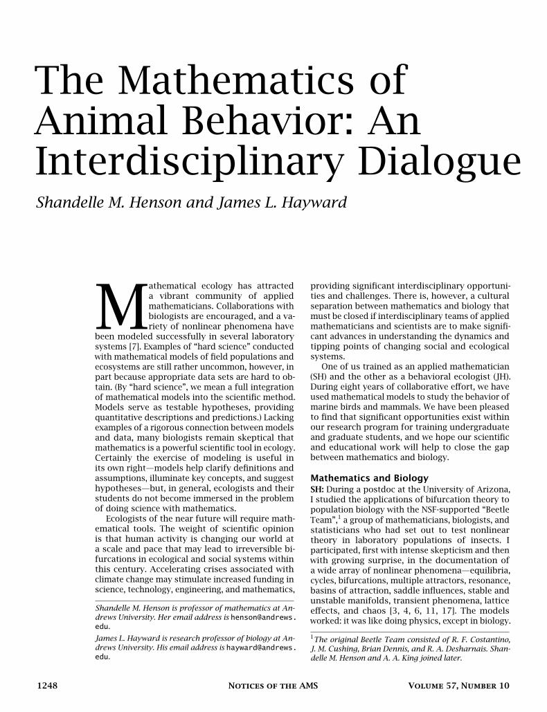
JH: Early in my professional career, in 1987,ethologist Joe Galusha asked me to join him doingresearch on a large glaucous-winged gull (Larusglaucescens) colony at Protection Island NationalWildlife Refuge in the Strait of Juan de Fuca,Washington (Figures 1, 2). Ethology is the studyof animal behavior in the natural habitat, andgulls are important animal models in ethology andbehavioral ecology. Since then I have spent muchof each summer on Protection Island collectingdata. Although most behavioral ecologists samplewith a view toward statistical analysis, I oftenhave collected long, temporally dense time seriesbecause I wanted to understand dynamics. Mycolleagues were amused; one joked, “Don’t youknow how to sample?” By the time I met Shandelle,I had many long time series but no satisfactoryway to analyze them statistically.

SH: Jim’s colleagues may have found his meth-ods of data collection excessive, but I was delighted.The long time series were just right for parame-terizing dynamic models. We pulled together theinterdisciplinary “Seabird Ecology Team”,2 appliedfor a grant from the National Science Foundation,and set out to try to replicate some of the laboratorysuccesses of the Beetle Team in the field.

JH: As a first step in our collaboration, I wantedto model the number of glaucous-winged gulls“loafing” on a pier adjacent to the breeding colony(Figure 3A). Loafing in birds is a general state ofimmobility involving behaviors such as sleeping,sitting, standing, resting, preening, and defecating.Loafing is of practical importance because it oftenconflicts with human interests. Gull feces containlandfill contaminants, erode roofing materials,spread Salmonella, and foul buildings, boats, andpiers. Gulls often loaf on airport runways, fromwhich they fly up and collide with aircraft. Such“bird strikes” result in expensive repairs and lossof human life. An ability to predict the incidence ofloafing with a mathematical model would providea first step toward the amelioration of bird/humanconflicts. The first time Shandelle and I discussedthe problem, she asked me to name the mostimportant variables influencing the dynamics ofloafing in these gulls. I started listing everythingthat I thought was important, but she cut meoff and insisted that I name only the two mostimportant variables. I argued vigorously against

2James L. Hayward, Shandelle M. Henson, Joseph G.Galusha, and J. M. Cushing: http://www.andrews.edu/~henson/seabird/.

Figure 1. Protection Island National WildlifeRefuge lies at the southeast end of the Straitof Juan de Fuca, Washington. Approximately70 percent of the breeding seabirds inWashington’s inland seaways nest here. Therefuge is closed to the public.

this but finally named tide height and time of day.I didn’t think it was possible that a model based onsuch limited information could describe or predictthe dynamics.

SH: In fact, the model based on these twovariables didn’t quite work, and Jim insisted thatwe had to include the day of the year. We did soand got a beautiful correspondence between modeland data [12]. One should begin with a simplemodel and add complications only as necessary.

JH: We parameterized and validated the modelon historical data and then made predictions forthe next field season. We took two undergraduatestudents to Protection Island, and the four of uscollected hourly data seventeen hours a day fortwenty-nine consecutive days. The correspondencebetween the a priori model predictions and actualfluctuations was remarkable [12] (Figure 3B-D).

SH: In a subsequent study [9] we tested theportability of the loafing model. On Protection

November 2010 Notices of the AMS 1249

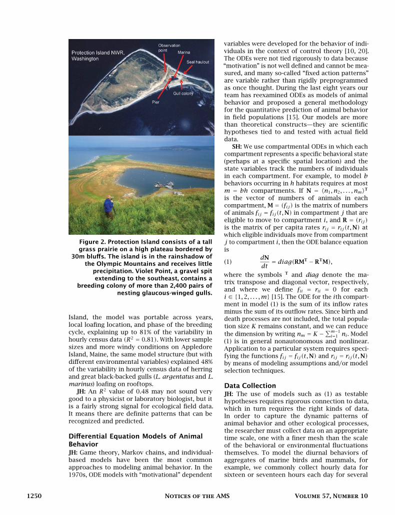
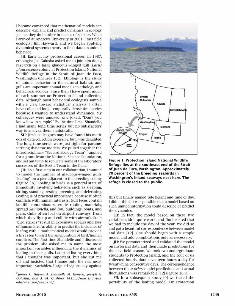
Figure 2. Protection Island consists of a tallgrass prairie on a high plateau bordered by

30m bluffs. The island is in the rainshadow ofthe Olympic Mountains and receives little

precipitation. Violet Point, a gravel spitextending to the southeast, contains a

breeding colony of more than 2,400 pairs ofnesting glaucous-winged gulls.

Island, the model was portable across years,local loafing location, and phase of the breedingcycle, explaining up to 81% of the variability inhourly census data (R2 = 0.81). With lower samplesizes and more windy conditions on AppledoreIsland, Maine, the same model structure (but withdifferent environmental variables) explained 48%of the variability in hourly census data of herringand great black-backed gulls (L. argentatus and L.marinus) loafing on rooftops.

JH: An R2 value of 0.48 may not sound verygood to a physicist or laboratory biologist, but itis a fairly strong signal for ecological field data.It means there are definite patterns that can berecognized and predicted.

Differential Equation Models of AnimalBehaviorJH: Game theory, Markov chains, and individual-based models have been the most commonapproaches to modeling animal behavior. In the1970s, ODE models with “motivational” dependent

variables were developed for the behavior of indi-viduals in the context of control theory [10, 20].The ODEs were not tied rigorously to data because“motivation” is not well defined and cannot be mea-sured, and many so-called “fixed action patterns”are variable rather than rigidly preprogrammedas once thought. During the last eight years ourteam has reexamined ODEs as models of animalbehavior and proposed a general methodologyfor the quantitative prediction of animal behaviorin field populations [15]. Our models are morethan theoretical constructs—they are scientifichypotheses tied to and tested with actual fielddata.

SH: We use compartmental ODEs in which eachcompartment represents a specific behavioral state(perhaps at a specific spatial location) and thestate variables track the numbers of individualsin each compartment. For example, to model bbehaviors occurring in h habitats requires at mostm = bh compartments. If N = 〈n1, n2, . . . , nm〉Tis the vector of numbers of animals in eachcompartment, M = (fij) is the matrix of numbersof animals fij = fij(t,N) in compartment j that areeligible to move to compartment i, and R = (rij)is the matrix of per capita rates rij = rij(t,N) atwhich eligible individuals move from compartmentj to compartment i, then the ODE balance equationis

(1)dN

dt= diag(RMT − RTM),

where the symbols T and diag denote the ma-trix transpose and diagonal vector, respectively,and where we define fii = rii = 0 for eachi ∈ {1,2, . . . ,m} [15]. The ODE for the ith compart-ment in model (1) is the sum of its inflow ratesminus the sum of its outflow rates. Since birth anddeath processes are not included, the total popula-tion size K remains constant, and we can reducethe dimension by writing nm = K −

∑m−1i=1 ni . Model

(1) is in general nonautonomous and nonlinear.Application to a particular system requires speci-fying the functions fij = fij(t,N) and rij = rij(t,N)by means of modeling assumptions and/or modelselection techniques.

Data CollectionJH: The use of models such as (1) as testablehypotheses requires rigorous connection to data,which in turn requires the right kinds of data.In order to capture the dynamic patterns ofanimal behavior and other ecological processes,the researcher must collect data on an appropriatetime scale, one with a finer mesh than the scaleof the behavioral or environmental fluctuationsthemselves. To model the diurnal behaviors ofaggregates of marine birds and mammals, forexample, we commonly collect hourly data forsixteen or seventeen hours each day for several

1250 Notices of the AMS Volume 57, Number 10

Figure 3. The loafing model depends on the (nondimensionalized and scaled) tide height T(t),solar elevation S(t), and a seasonal envelope Kp(t) that depends on day of year. A. Gulls loafingon the pier. B. Model prediction (red), data from spring 2002 (circles), and tide height (blue). Eachdaily panel is identified with the day of the year. Each row of 14 panels corresponds to one2-week tidal cycle. Tidal nodes (N) occur on or near days 142 and 155. Each column of panelscontains similar patterns in data. C. Model predictions for the spring of 2002. Oscillations arepresent on daily, biweekly, and yearly time scales. The dotted curve is the yearly envelopeoscillation Kp(t). D. Data observations corresponding to the predictions in C. E. Tidal oscillationfor the data collection time period in 2002. The tidal nodes are indicated with arrows.

weeks at a time, since the aggregate dynamics andenvironmental conditions do not change muchduring one hour. Student research assistants makesuch dense data collection possible. Furthermore, itis best to collect enough data so that some can be setaside for the purposes of model validation. Animalbehavior is an excellent candidate for rigorousdynamic modeling. Obviously it could take monthsor years to collect long time series at the populationlevel. For example, the generation time of the flourbeetle Tribolium castaneum studied by the BeetleTeam is about four weeks, and the chaotic Triboliumtime series reported in Science spanned eightyweeks [2].3 To collect an analogous data set for a

3Experimental/mathematical ecologist Bob Costantinocontinued the study for nearly eight years (ninety-sevengenerations), producing one of the longest population timeseries in ecology.

population of glaucous-winged gulls (generationtime about four years) would require eighty years.

Connecting Models to DataSH: Parameterization requires a stochastic versionof the model that properly accounts for the noisestructure of the particular system. For example, inthe systems we discuss in this article, stochasticperturbations are largely uncorrelated in hourlysample times. We take stroboscopic snapshots

(2) Nτ+1 = F(τ,Nτ)of the continuous-time system at the hourly sampletimes τ = 0,1,2, . . . , where Nτ = N(τ) and

(3) F(τ,Nτ) = Nτ +∫ τ+1

τdiag(RMT − RTM)dt.

The stochastic model is

(4) φ(Nτ+1) = φ(F(τ,Nτ))+ Eτ .

November 2010 Notices of the AMS 1251

Here φ is a variance-stabilizing transformationthat renders noise approximately additive on theφ-scale, and Eτ is a vector from a multivariate nor-mal random distribution with variance-covariancematrix Σ.

Given an observed sequence {nτ}qτ=0 of datavectors, the “conditioned one-step” model pre-diction for the next observation at time τ + 1 isNτ+1 = F(τ,nτ). The (transformed) residual erroris

(5) φ(nτ+1)−φ(Nτ+1) = φ(nτ+1)−φ(F(τ,nτ)).Model (4) assumes the residuals come from a jointnormal distribution and are uncorrelated in sampletime. The likelihood that the residuals arose fromsuch a distribution can be expressed as a functionof the model parameters. The maximizer of thelikelihood function is the vector of parameterestimates [4].

Two main sources of noise in ecological systemsare “demographic” and “environmental”. Demo-graphic stochasticity is experienced independentlyby single individuals or small subsets of individuals,whereas environmental stochasticity is experiencedby all individuals in a population [4]. Noise in agiven system can be primarily demographic, pri-marily environmental, or a mixture of the two.The transformations φ(x) = lnx and φ(x) = √xrender environmental and demographic noise, re-spectively, approximately additive [4]. Anothertransformation, φ(x,ψ), constructed by statisti-cian Brian Dennis and dynamicist J. M. Cushing,parses out the relative effects of environmentaland demographic noise through the estimation ofa parameter ψ ∈ (0,1] that yields φ(x,1) = lnxand limψ→0+ φ(x,ψ) =

√x [15].

Model ValidationJH: A good model not only describes and explains,but also predicts; otherwise modeling is merelya curve-fitting exercise. Model validation is abouttesting model predictability on a data set not usedto estimate the parameters.

SH: One way to validate a model is to randomlydivide a data set into “estimation data” and “vali-dation data”. First, estimate the model parametersusing the estimation data. The goodness-of-fit(to the estimation data) can be computed with ageneralized R2

(6) R2 = 1−∑qτ=1(φ(nτ)−φ(Nτ))2∑qτ=1(φ(nτ)−φ(n))2

where nτ and Nτ are, respectively, the observedand predicted values at time τ and φ(n) is thesample mean of the transformed observations[4]. Second, compute the goodness-of-fit for thevalidation data without reestimating parametersand compare this with the goodness-of-fit for theestimation data.

JH: The most convincing models are thosefurther tested by making a priori predictions thatare then borne out by new experiments. Unexpectedpredictions are ideal opportunities for testing amodel. For example, the loafing model predicted,successfully, that the lowest numbers of gullswould occur at high tide on days corresponding totidal nodes (Figure 3B, days 142 and 155). This iscontrary to previously published assertions, basedon data averaging, that the lowest numbers occurnear low tide. While it is true that gulls tend to beaway foraging at low tide, it is also true that gullstend to return to loafing sites in the morning andevening. In the previous studies, data averagingmasked the effect of time of day, whereas themodeling approach made it possible to predict lowloafing numbers at high tides that occurred in themiddle of the day.

Model SelectionSH: If mathematical models are to serve as testablehypotheses, there must be a way to test alternativehypotheses. Information theoretic methods suchas the Akaike information criterion (AIC) are ideallysuited for choosing the best model from a suite ofalternatives [1]. The AIC takes into account boththe value of the likelihood function and the numberof parameters, penalizing models for overfitting:

(7) AIC = −2 lnL+ 2κ,

where L is the likelihood value for the (fitted) modelandκ is the number of model parameters (includingthe variance of the likelihood function as estimatedfrom the residuals) [1]. Model comparison is basedon the rank of AIC values for each model, with thesmallest AIC indicating the best model.

JH: We used information theoretic model selec-tion techniques to determine the environmentaldrivers of harbor seal (Phoca vitulina) hauloutduring the pupping season on Protection Island[8] (Figure 4C). Seals “haul out” on the beachesof Protection Island by the hundreds, where theyremain safe from killer whales, rest from feeding,and give birth to offspring. Harbor seal numbersare monitored closely by governmental authoritiesin both Europe and North America, and optimalcensus times occur when they are hauled out. Alist of alternative hypotheses for environmentalhaulout cues gave rise to a suite of twenty-threealternative models. The best model (with lowestAIC) was a function of tide height and direction ofthe current and explained 40% of the variability inhourly census data (R2 = 40; Figure 4A). The modelshowed that, at this pupping site, managers canexpect maximal daily haulouts to occur during re-ceding tides, approximately midway between highand low tides. This may be because food availabilityis lowest when the current is strongest during re-ceding tides and peaks during the maximal currentduring incoming tides, which corresponds with

1252 Notices of the AMS Volume 57, Number 10

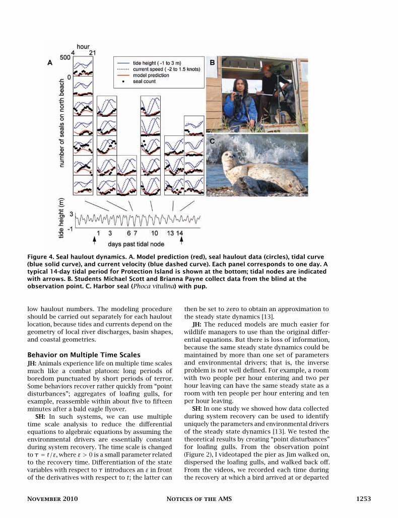
Figure 4. Seal haulout dynamics. A. Model prediction (red), seal haulout data (circles), tidal curve(blue solid curve), and current velocity (blue dashed curve). Each panel corresponds to one day. Atypical 14-day tidal period for Protection Island is shown at the bottom; tidal nodes are indicatedwith arrows. B. Students Michael Scott and Brianna Payne collect data from the blind at theobservation point. C. Harbor seal (Phoca vitulina) with pup.

low haulout numbers. The modeling procedureshould be carried out separately for each hauloutlocation, because tides and currents depend on thegeometry of local river discharges, basin shapes,and coastal geometries.

Behavior on Multiple Time ScalesJH: Animals experience life on multiple time scalesmuch like a combat platoon: long periods ofboredom punctuated by short periods of terror.Some behaviors recover rather quickly from “pointdisturbances”; aggregates of loafing gulls, forexample, reassemble within about five to fifteenminutes after a bald eagle flyover.

SH: In such systems, we can use multipletime scale analysis to reduce the differentialequations to algebraic equations by assuming theenvironmental drivers are essentially constantduring system recovery. The time scale is changedto τ = t/ε, where ε > 0 is a small parameter relatedto the recovery time. Differentiation of the statevariables with respect to τ introduces an ε in frontof the derivatives with respect to t ; the latter can

then be set to zero to obtain an approximation tothe steady state dynamics [13].

JH: The reduced models are much easier forwildlife managers to use than the original differ-ential equations. But there is loss of information,because the same steady state dynamics could bemaintained by more than one set of parametersand environmental drivers; that is, the inverseproblem is not well defined. For example, a roomwith two people per hour entering and two perhour leaving can have the same steady state as aroom with ten people per hour entering and tenper hour leaving.

SH: In one study we showed how data collectedduring system recovery can be used to identifyuniquely the parameters and environmental driversof the steady state dynamics [13]. We tested thetheoretical results by creating “point disturbances”for loafing gulls. From the observation point(Figure 2), I videotaped the pier as Jim walked on,dispersed the loafing gulls, and walked back off.From the videos, we recorded each time duringthe recovery at which a bird arrived at or departed

November 2010 Notices of the AMS 1253

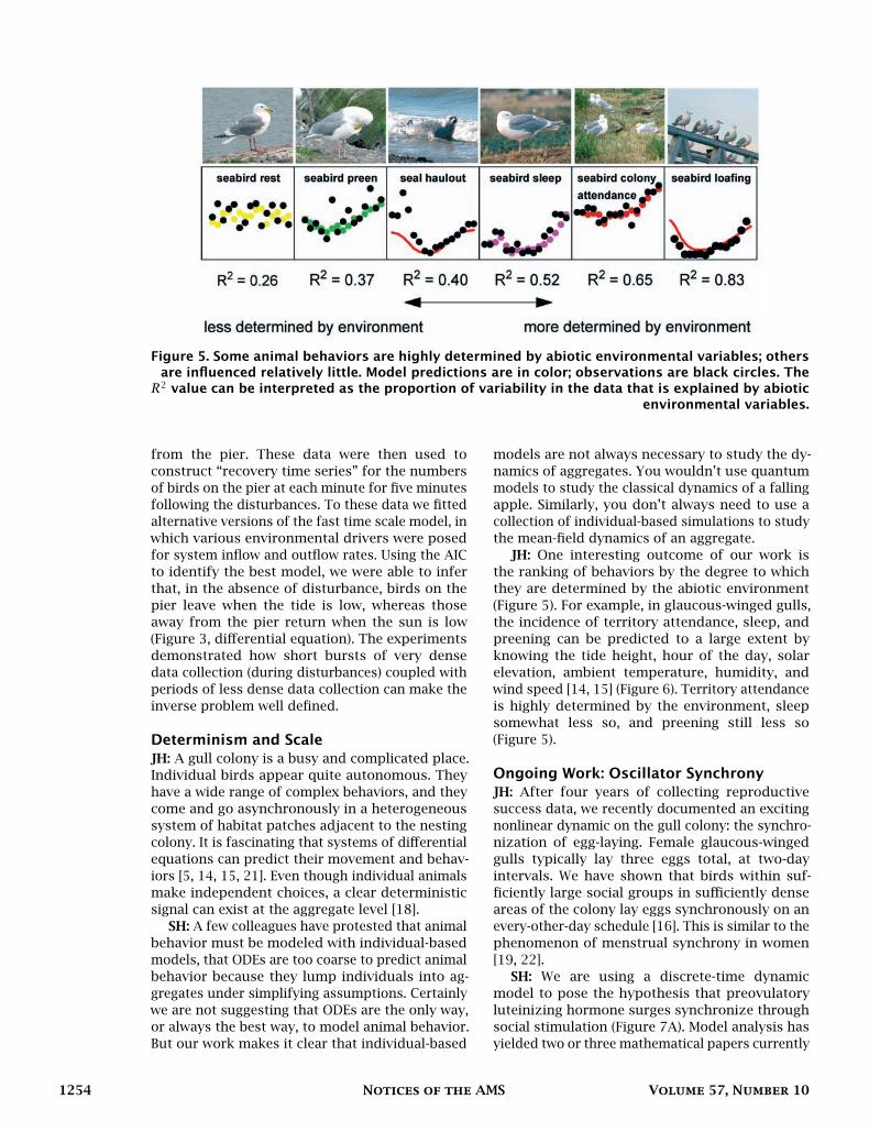
Figure 5. Some animal behaviors are highly determined by abiotic environmental variables; othersare influenced relatively little. Model predictions are in color; observations are black circles. TheR2 value can be interpreted as the proportion of variability in the data that is explained by abiotic

environmental variables.

from the pier. These data were then used toconstruct “recovery time series” for the numbersof birds on the pier at each minute for five minutesfollowing the disturbances. To these data we fittedalternative versions of the fast time scale model, inwhich various environmental drivers were posedfor system inflow and outflow rates. Using the AICto identify the best model, we were able to inferthat, in the absence of disturbance, birds on thepier leave when the tide is low, whereas thoseaway from the pier return when the sun is low(Figure 3, differential equation). The experimentsdemonstrated how short bursts of very densedata collection (during disturbances) coupled withperiods of less dense data collection can make theinverse problem well defined.

Determinism and ScaleJH: A gull colony is a busy and complicated place.Individual birds appear quite autonomous. Theyhave a wide range of complex behaviors, and theycome and go asynchronously in a heterogeneoussystem of habitat patches adjacent to the nestingcolony. It is fascinating that systems of differentialequations can predict their movement and behav-iors [5, 14, 15, 21]. Even though individual animalsmake independent choices, a clear deterministicsignal can exist at the aggregate level [18].

SH: A few colleagues have protested that animalbehavior must be modeled with individual-basedmodels, that ODEs are too coarse to predict animalbehavior because they lump individuals into ag-gregates under simplifying assumptions. Certainlywe are not suggesting that ODEs are the only way,or always the best way, to model animal behavior.But our work makes it clear that individual-based

models are not always necessary to study the dy-namics of aggregates. You wouldn’t use quantummodels to study the classical dynamics of a fallingapple. Similarly, you don’t always need to use acollection of individual-based simulations to studythe mean-field dynamics of an aggregate.

JH: One interesting outcome of our work isthe ranking of behaviors by the degree to whichthey are determined by the abiotic environment(Figure 5). For example, in glaucous-winged gulls,the incidence of territory attendance, sleep, andpreening can be predicted to a large extent byknowing the tide height, hour of the day, solarelevation, ambient temperature, humidity, andwind speed [14, 15] (Figure 6). Territory attendanceis highly determined by the environment, sleepsomewhat less so, and preening still less so(Figure 5).

Ongoing Work: Oscillator SynchronyJH: After four years of collecting reproductivesuccess data, we recently documented an excitingnonlinear dynamic on the gull colony: the synchro-nization of egg-laying. Female glaucous-wingedgulls typically lay three eggs total, at two-dayintervals. We have shown that birds within suf-ficiently large social groups in sufficiently denseareas of the colony lay eggs synchronously on anevery-other-day schedule [16]. This is similar to thephenomenon of menstrual synchrony in women[19, 22].

SH: We are using a discrete-time dynamicmodel to pose the hypothesis that preovulatoryluteinizing hormone surges synchronize throughsocial stimulation (Figure 7A). Model analysis hasyielded two or three mathematical papers currently

1254 Notices of the AMS Volume 57, Number 10

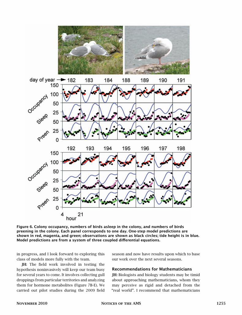
Figure 6. Colony occupancy, numbers of birds asleep in the colony, and numbers of birdspreening in the colony. Each panel corresponds to one day. One-step model predictions areshown in red, magenta, and green; observations are shown as black circles; tide height is in blue.Model predictions are from a system of three coupled differential equations.

in progress, and I look forward to exploring thisclass of models more fully with the team.

JH: The field work involved in testing thehypothesis noninvasively will keep our team busyfor several years to come. It involves collecting gulldroppings from particular territories and analyzingthem for hormone metabolites (Figure 7B-E). Wecarried out pilot studies during the 2009 field

season and now have results upon which to baseour work over the next several seasons.

Recommendations for MathematiciansJH: Biologists and biology students may be timidabout approaching mathematicians, whom theymay perceive as rigid and detached from the“real world”. I recommend that mathematicians

November 2010 Notices of the AMS 1255

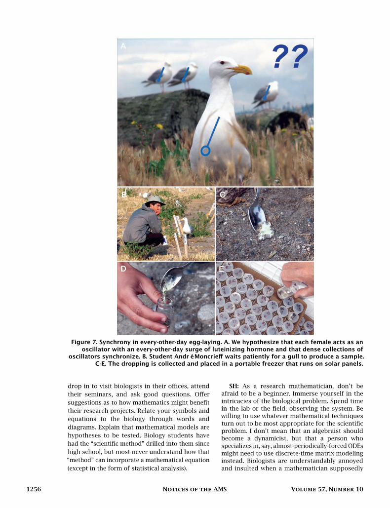
Figure 7. Synchrony in every-other-day egg-laying. A. We hypothesize that each female acts as anoscillator with an every-other-day surge of luteinizing hormone and that dense collections of

oscillators synchronize. B. Student André Moncrieff waits patiently for a gull to produce a sample.C-E. The dropping is collected and placed in a portable freezer that runs on solar panels.

drop in to visit biologists in their offices, attendtheir seminars, and ask good questions. Offersuggestions as to how mathematics might benefittheir research projects. Relate your symbols andequations to the biology through words anddiagrams. Explain that mathematical models arehypotheses to be tested. Biology students havehad the “scientific method” drilled into them sincehigh school, but most never understand how that“method” can incorporate a mathematical equation(except in the form of statistical analysis).

SH: As a research mathematician, don’t beafraid to be a beginner. Immerse yourself in theintricacies of the biological problem. Spend timein the lab or the field, observing the system. Bewilling to use whatever mathematical techniquesturn out to be most appropriate for the scientificproblem. I don’t mean that an algebraist shouldbecome a dynamicist, but that a person whospecializes in, say, almost-periodically-forced ODEsmight need to use discrete-time matrix modelinginstead. Biologists are understandably annoyedand insulted when a mathematician supposedly

1256 Notices of the AMS Volume 57, Number 10

“collaborates” but is really only looking for theperfect application of his or her pet theorems.While you are becoming a scientist, always remaina mathematician; keep publishing your own workin mathematics journals. Projects that involve realdata and intense interdisciplinary collaborativeeffort take a long time to mature, so keep yourown independent work going in the meantime.

JH: Be patient with your biologist colleagues.It will take time for them to enter your world ofsymbolic language and precise deduction. You maybe frustrated by a field ecologist’s global thinkingabout a problem, but he or she may think you naivewhen you want to reduce the problem to a handfulof variables.

SH: Drop any feelings of superiority you mighthave as a mathematician. Remember, mathematicsis a simplification of the “real world”, not viceversa. The universe is a complex place, and thereare plenty of scientific problems that will give youa vigorous intellectual workout if you are willingto engage them.

PostscriptIt is not our purpose here to list all of the researchgroups, institutes, meeting venues, or journalsinvolved in the rigorous connection of mathemati-cal models to ecological field data. The interestedreader might begin, however, with the bark beetlecollaboration of James Powell of Utah State Univer-sity and Jesse Logan of the USDA-Forest Service;4

the green tree frog collaboration of Azmy Acklehof the University of Louisiana at Lafayette with theUSGS National Wetlands Research Center,5 and thevarious projects of Mark Lewis’s group at the Uni-versity of Alberta.6 NSF-funded institutes such asthe National Institute for Mathematical and Biolog-ical Synthesis (NIMBioS),7 located at the Universityof Tennessee, and the Mathematical BiosciencesInstitute (MBI),8 located at Ohio State University,bring mathematicians and biologists together ininterdisciplinary collaboration and training of stu-dents. The Joint Mathematics Meetings have hostedspecial sessions in this area for several years, anda number of journals are specifically interestedin this type of work, including Natural ResourceModeling, the Journal of Biological Dynamics, andthe Bulletin of Mathematical Biology. An expandedversion of this article that includes information onpedagogy and research training of undergraduateand master’s students is online.9

4http://www.math.usu.edu/~powell/.5http://www.ucs.louisiana.edu/~asa5773/ubm/index.html.6http://www.math.ualberta.ca/~mlewis/.7http://www.nimbios.org/.8http://mbi.osu.edu/.9http://www.andrews.edu/~henson/HensonHayward2010.pdf.

AcknowledgmentsWe thank the National Science Foundation (DMS0314512 and DMS 0613899) and Andrews Univer-sity (faculty grants 2002–2010); fellow Seabird andBeetle Team members J. M. Cushing, J. G. Galusha,R. F. Costantino, R. A. Desharnais, B. Dennis, andA. A. King; K. Ryan, Project Director of the Wash-ington Maritime National Wildlife Refuge Complex,U.S. Fish and Wildlife Service, for permission towork on Protection Island; Rosario Beach MarineLaboratory for logistical support; and our manystudent field assistants.

References[1] K. P. Burnham and D. R. Anderson, Model Selection

and Multi-Model Inference: A Practical Information-Theoretic Approach, Second Edition, Springer, NewYork, 2002.

[2] R. F. Costantino, R. A. Desharnais, J. M. Cush-ing, and B. Dennis, Chaotic dynamics in an insectpopulation, Science 275 (1997), 389–391.

[3] R. F. Costantino, R. A. Desharnais, J. M. Cushing,B. Dennis, S. M. Henson, and A. A. King, Nonlinearstochastic population dynamics: The flour beetleTribolium as an effective tool of discovery. In R. A.Desharnais (ed.), Population Dynamics and Labora-tory Ecology, Academic Press, New York, 2005, pp.101–141.

[4] J. M. Cushing, R. F. Costantino, B. Dennis, R. A. De-sharnais, and S. M. Henson, Chaos in Ecology:Experimental Nonlinear Dynamics, Academic Press,San Diego, 2003.

[5] S. P. Damania, K. W. Phillips, S. M. Henson, andJ. L. Hayward, Habitat patch occupancy dynamicsof glaucous-winged gulls (Larus glaucescens) II: Acontinuous-time model, Nat. Resource Modeling 18(2005), 469–499.

[6] B. Dennis, R. A. Desharnais, J. M. Cushing,S. M. Henson, and R. F. Costantino, Estimatingchaos and complex dynamics in an insect population,Ecol. Monogr. 71 (2001), 277–303.

[7] R. A. Desharnais, ed., Population Dynamics andLaboratory Ecology, Academic Press, New York,2005.

[8] J. L. Hayward, S. M. Henson, C. J. Logan, C. R. Par-ris, M. W. Meyer, and B. Dennis, Predicting numbersof hauled-out harbour seals: A mathematical model,J. Appl. Ecol. 42 (2005), 108–117.

[9] J. L. Hayward, S. M. Henson, R. D. Tkachuck,C. M. Tkachuck, B. G. Payne, and C. K. Boothby,Predicting gull/human conflicts with mathemati-cal models: A tool for management, Nat. ResourceModeling 22 (2009), 544–563.

[10] B. A. Hazlett and C. E. Bach, Predicting behavioralrelationships. In B. A. Hazlett, (ed.), QuantitativeMethods in the Study of Animal Behavior, AcademicPress, New York, 1977, pp. 121–144.

[11] S. M. Henson, R. F. Costantino, J. M. Cushing,R. F. Desharnais, B. Dennis, and A. A. King, Latticeeffects observed in chaotic dynamics of experimentalpopulations, Science 294 (2001), 602–605.

[12] S. M. Henson, J. L. Hayward, C. M. Burden, C. J. Lo-gan, and J. G. Galusha, Predicting dynamics ofaggregate loafing behavior in glaucous-winged gulls

November 2010 Notices of the AMS 1257

Help bring E WORLD

hematics ives of

ople.

HHHHHHHHHHHHHHHHHeeeeelllllllllllllllllppppppppppppppppppp bbbbbbbbbbbbbbbbbbbbrrrrrrrrrrriiiiiiiiiiiinnnnnnnnnggggggggggggggggg EEEEEEEEEEE WWWWWWWWWWWWWWWWWWWWWWWOOOOOOOOOOOOOOOOOOOOOOOORRRRRRRRRRRRRRRRRRLLLLLLLLLLLLLDDDDDDDDDDDD

hhhhhhhhhhhhhhhheeeeeeeemmmmmmmmmmmmmaaaaaaaaaaaaaaaattttttttttttttttttttttttttttttttttttttttttiiiiiiiiiiiiiiiiiiiiiiiiiiiiiiiiiiiiiiiiiiiccccccccccccccccccccccccccccccccccccsssssssssssss iiiiiiiiiiiivvvvvvvvvvvveeeeeeeeeeeeeeeeeeeeeeeesssssssssssssssssssssssssssssss ooooooooooooooooooooooooooooooooooooooooooooooooofffffffffffffffffffffffffffffff

ooooooooooooooooooooooooooooooooooooooooooooooooooooooooooooooooppppppppppppppppppppppppppppppppppppppppppppppppppppppppppppppppppppppppppppppppppppppppppppppppppppppplllllllllllllllllllllllllllllllllllleeeeeeeee.....

Help bring THE WORLDof mathematicsinto the lives of young people.

Whether they become scientists, engineers, or entrepreneurs, young people with mathematical talent need to be nurtured. Income from this fund supports the Young Scholars Program, which provides grants to summer programs for talented high school students.

Please give generously.Learn about giving opportunities and estate planningwww.ams.org/giving-to-ams

Contact the AMS Development Office 1.800.321.4267 (U.S. and Canada) or 1.401.455.4000 (worldwide)email: development@ams.org

09/04

n a

The AMS

Epsilon Fundfor Young Scholars

(Larus glaucescens) at a Washington colony, Auk 121(2004), 380–390.

[13] S. M. Henson, J. L. Hayward, and S. P. Damania,Identifying environmental determinants of diurnaldistribution in marine birds and mammals, Bull.Math. Biol. 68 (2006), 467–482.

[14] S. M. Henson, J. G. Galusha, J. L. Hayward, andJ. M. Cushing, Modeling territory attendance andpreening behavior in a seabird colony as functions ofenvironmental conditions, J. Biol. Dynamics 1 (2007),95–107.

[15] S. M. Henson, B. Dennis, J. L. Hayward, J. M. Cush-ing, and J. G. Galusha, Predicting the dynamics ofanimal behaviour in field populations, Anim. Behav.74 (2007), 103–110.

[16] S. M. Henson, J. L. Hayward, J. M. Cushing, andJ. G. Galusha, Socially-induced synchronization ofevery-other-day egg laying in a seabird colony, Auk127 (2010), 571-580.

[17] A. A. King, R. F. Costantino, J. M. Cushing,S. M. Henson, R. A. Desharnais, and B. Dennis,Anatomy of a chaotic attractor: Subtle model-predicted patterns revealed in population data, Proc.Nat. Acad. Sci. 101 (2004), 408–413.

[18] S. A. Levin, The problem of pattern and scale inecology, Ecology 73 (1992), 1943–1947.

[19] M. K. McClintock, Menstrual synchrony andsuppression, Nature 229 (1971), 244–245.

[20] D. J. McFarland, Feedback Mechanisms in AnimalBehaviour, Academic Press, London, 1971.

[21] A. L. Moore, S. P. Damania, S. M. Henson, andJ. L. Hayward, Modeling the daily activities of breed-ing colonial seabirds: Dynamic occupancy patternsin multiple habitat patches, Math. Biosci. Eng. 5(2008), 831–842.

[22] S. Strogatz, Sync: The Emerging Science ofSpontaneous Order, Hyperion, New York, 2003.

Note: The aerial image at the top of Figure 2 iscourtesy of the Washington Department of Trans-portation. All the other figures are collaborativeefforts of the authors.

1258 Notices of the AMS Volume 57, Number 10