1

The mathematical structure of thermodynamics

Peter Salamon1, Bjarne Andresen2, James Nulton1, Andrzej K. Konopka3,1

1 – San Diego State University Department of Mathematics & Statistics San Diego, CA USA 92182-7720 2 – Niels Bohr Institute Universitetsparken 5 DK-2100 Copenhagen Ø Denmark 3 – BioLinguaSM Reasearch, Inc. CASSA Center 10331 Battleridge Place Gaithersburg, MD USA Introduction Thermodynamics is unique among physical and chemical descriptions of our surroundings in that it does not rely on a detailed knowledge of any interior structure of the systems1 to which it pertains but rather treats such systems as “black boxes” whose equilibrium states are determined by the surroundings with which they can coexist and which can be described by a few parameters. This feature assures that the theory holds true when the system is a collection of molecules, or a beaker of water, or a black hole. Einstein expressed this feature of thermodynamic theory in his classic quote:

"Thermodynamics is the only physical theory of universal content which, within the framework of the applicability of its basic concepts, I am convinced will never be overthrown." — Albert Einstein

Foremost among these basic concepts is the notion of equilibrium, the situation where the state of the system does not vary noticeably in time. The “noticeably” in the previous sentence has two complications. The first is that if this system were to be cut off from its surroundings the state would remain the same. This distinguishes equilibria from steady states. The second is the fact that the notion of equilibrium is associated with a particular time scale. Over larger periods of time, any system will eventually evolve until the final dead state of 56Fe is reached through nuclear transformations. 1 In standard presentations of thermodynamics (see for example [2, 5]), the term thermodynamic system is universally used. In order not to deviate from this established usage we have retained the expression here in spite of the collision of meanings of the overloaded term system in this handbook. Every occurrence of the term system in this chapter is to be taken in the thermodynamic sense.

2

As an example, consider a carbon filament suspended in air. On a human timescale, that carbon filament will be in equilibrium thermally with the air surrounding it while retaining its chemical integrity as free carbon. On a much longer timescale, it would also achieve chemical equilibrium with the oxygen of the surroundings to form CO2. If we were to pass an electric current through the filament, it would heat up and glow and appear not to change over many minutes. While this would be a steady state on this timescale, it is not equilibrium since when we stop the current, the state changes to a lower temperature. A Historical Introduction to Thermodynamics Thermodynamics began with the development of early theories of heat and mechanics. The analysis was primarily motivated by an economic impetus: the newly invented steam engine. Carnot’s [1] great accomplishment was to show that the conversion of heat into work has limitations set by what we today view as a “no free lunch” principle: one cannot extract more work from an initial configuration of states of a collection of thermodynamic systems than it would take to restore those systems to such initial states after the work was extracted (see for instance [2]). This is often stated as the impossibility of a perpetual motion machine of the second kind [2] since it is the essence of what we today call the second law of thermodynamics. It predates the first law by about 25 years. The first law of thermodynamics also can be stated as a “no free lunch” principle: we cannot get more work out of a system than the change in its internal energy. More commonly however, the first law is stated as a conservation law which, historically, combined the two separate conservation laws for heat (caloric) and mechanical energy [3] into one conservation law for a quantity called internal energy whose change is defined by QWU +=! , (1) where U is the internal energy, W is the work done on the system and Q is the heat added to the system. The fact that this defines a conserved quantity is a consequence of an empirical observation – a given amount of work turned into heat by friction always produces the same amount of heat. (Here as well as in the following we only consider the exchange of heat and work with the surroundings except where explicitly stated otherwise for simplicity.) Since heat and work are conserved in processes where no interconversion takes place, this means that internal energy U will be conserved even in processes including such conversions. The fact that U is a function of state is not obvious but requires an assumption to this effect. It is physically stated in terms of cyclic processes, i.e. processes in which a system starts and ends in the same state. For such processes, the work produced by the system to the surroundings must equal the heat withdrawn from the surroundings. A Carnot cycle, and a Stirling cycle [4] are examples of such cycles.

3

Energy has become firmly rooted in our language and intuition, and the conservation of this energy, as stated by the first law of thermodynamics, is so widely applied that the subtleties associated with it have faded from the collective consciousness. The second law on the other hand carries a great deal of subtlety. It is associated with a far lesser known quantity called entropy that most people, even many scientists, find difficult and abstruse. The deeper meaning of the second law is a unidirectionality associated with physical processes and as such occupies a unique and important position among physical laws. All other physical laws view a process and its time reversed version as equally acceptable or unacceptable on physical grounds. The second law of thermodynamics asserts that only one direction is physically possible – unless of course the process is reversible, which is only an ideal abstraction. The second law is associated with the increase of entropy whose changes are defined by T/QS rev!! = . (2) Here ΔS is the increase of entropy of a thermodynamic system at temperature T when the amount of heat ΔQrev is added reversibly. Intuitively, the construction of entropy (see [5]) expresses the unidirectionality of transport, notably of heat, between two systems, from higher to lower temperature. The mathematical theory of thermodynamic systems focuses on one such system, a thermodynamic system, and describes geometrically the set of equilibrium states it can have. The allowed modes of interaction with the surroundings define the equilibrium. Important for this perspective was a far subtler form of the second law introduced by Caratheodory [6], which asserts that arbitrarily close to any equilibrium state of a system there exist states that are not accessible without the transport of heat out of the system. Exchange of other quantities like work and mass can occur freely. Definitions and Axioms A simple thermodynamic system is a homogeneous macroscopic collection of components. The system is treated as a black box and its state is describable by a small number of macroscopic parameters, typically its energy, entropy, volume, and particle number, dictated by the surroundings with which it coexists. However, not all of these are necessarily independent. A simple single phase system consisting of n–1 components has n independent parameters, called thermodynamic degrees of freedom. Parameters in excess of this will be interdependent. Simple thermodynamic systems may interact with one another to form a non-uniform thermodynamic system. Such interactions between systems and between systems and the surroundings occur through walls which are constructed to allow passage of certain quantities. All other exchange is blocked. An isolated system has no exchange with its surroundings, i.e. its volume, energy, particle number etc. are fixed. An adiabatic wall allows passage of only volume (e.g. by moving a piston i.e. exchanging work, but no particles). A diathermal wall allows in addition passage of heat. Similarly, a semipermeable wall further allows passage of specific types of particles.

4

By selecting a proper wall, desired standard processes are allowed. Thus an adiabatic wall between a system and its surroundings allows only adiabatic processes, i.e. processes where no heat is exchanged with the surroundings and production of work therefore must be accompanied by a decrease of the internal energy. A diathermal wall permits isothermal processes at the temperature of the surroundings. Here work produced is compensated by influx of heat, keeping the internal energy fixed. Semipermeable walls may allow e.g. passage of oxygen, sodium ions, water, and/or glucose. Inside a system coupled to its surroundings through such a wall, chemical reactions may proceed while exchanging reactants and products with the surroundings. Thermodynamic cycles are made up of sequences of such standard processes. For example, a Carnot cycle involves a system (called the working fluid) which undergoes a cyclic process by following a sequence of standard processes while connected to a corresponding sequence of surroundings. The sequence followed is: isothermal (hot) – adiabatic – isothermal (cold) – adiabatic. Systems with ongoing chemical reactions may steer such reactions through the permeability of the wall and by controlling the work and heat flows (isothermal, adiabatic, isobaric etc.). The Carnot cycle also illustrates another important version of the second law – the fact that the conversion of heat to work is a limited affair in which only a certain fraction of the heat can be captured as work. How large a fraction can be converted is the so-called Carnot efficiency which depends on the temperatures of heat sources and sinks available for contact during the isothermal branches of the cycle. Let’s look at a simple reversible Carnot heat engine operating between a hot heat reservoir at temperature TH and a cold reservoir at TL. The engine absorbs the amount of heat QH from the hot reservoir accompanied by the entropy influx SH=QH/TH. Since the engine operates in a cycle and thus cannot accumulate entropy, it must somehow dispose of this much entropy. The work produced does not carry any entropy, so the only available sink is the cold heat reservoir. However, entropy and heat are transported together, so discharging SH must be accompanied by a discharge of heat equal to QL=SH×TL. The fraction of heat turned into work in this reversible machine is thus (QH–QL)/QH = 1–TL/TH, the famous Carnot efficiency. A realistic irreversible engine will of course produce even less work. Note that the engine cannot convert all incoming heat into work, not for energetic reasons but due to entropy constraints. In all cases the quantities exchanged belong to a class of variables called extensive, i.e. variables which are additive when systems are merged (energy, entropy, volume, particle number). The corresponding intensive variables (temperature, pressure, chemical potential) are not additive over sub-systems but describe possible gradients. At equilibrium either between systems or between a system and its environment these intensive variables will be the same in all the connected systems. Thus extensive variables scale with the power 1 of the size of the system considered, the intensive variables with power 0.

5

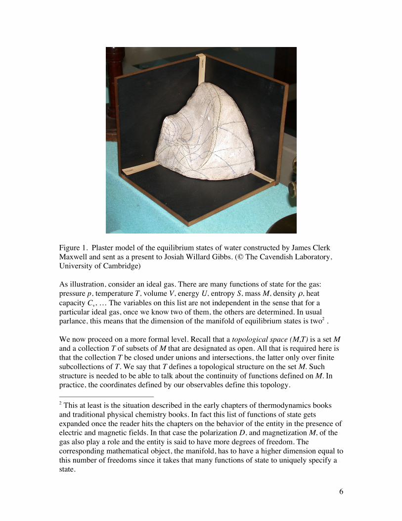
Using the definitions above, we are in a position to state the axioms in their traditional geometrical form [7]. Axiom 1: For any thermodynamic system, there exists an extensive function of state U called the internal energy. Axiom 2: For any thermodynamic system, there exists an extensive function of state S called the entropy. The entropy is a concave function of any set of complete independent extensive parameters of the system ),,,,,,,,( 21 KK MPNNNVUfS k= , where the arguments are the internal energy U, volume V, particle numbers N of the k molecular species, polarization P, magnetization M, as well as any other relevant extensive quantity. These two axioms are essentially the first and second laws expressed in terms of a single system. The geometrical picture that goes with this formulation is the concave surface S=f(U,V,…) in n+1 dimensions for the n degree of freedom system. The sections below present a modern differential geometrical alternative to this picture including a rigorous proof of Caratheodory’s principle. The presentation is perforce rather sketchy in that it provides the bare minimum of examples, although all the definitions are carefully stated and rigorous. More details can be found in any modern differential geometry book [8, 9]. Thermodynamic States, Coordinates, and Manifolds Roughly speaking, a manifold is a coordinatizable set. More correctly, it is a set equipped with real-valued coordinates which uniquely label the elements and whose values change in a “continuous” fashion. Historically, manifolds arose as a collection of variables subject to equations. Early examples were well studied by the founders of differential geometry as curves and surfaces [10]. Going to higher dimensions was an obvious and yet conceptually difficult leap that required a higher level of abstraction [11]. Spaces of states of dynamical systems were one strong impetus towards such abstraction. Mechanical systems, such as compound pendulums, provided ready examples. The set of equilibrium states of a thermodynamic system is yet another example. This is the example for the present chapter. The set of equilibrium states of a thermodynamic system was also conceptualized initially as a surface; James Clerk Maxwell had a plaster model of the equilibrium states of water constructed and sent it as a present to Josiah Willard Gibbs (see Figure 1), the pioneer responsible for the dramatic shift in point of view of thermodynamics from a theory of processes to a theory of equilibrium states [3].

6

Figure 1. Plaster model of the equilibrium states of water constructed by James Clerk Maxwell and sent as a present to Josiah Willard Gibbs. (© The Cavendish Laboratory, University of Cambridge) As illustration, consider an ideal gas. There are many functions of state for the gas: pressure p, temperature T, volume V, energy U, entropy S, mass M, density ρ, heat capacity Cv, … The variables on this list are not independent in the sense that for a particular ideal gas, once we know two of them, the others are determined. In usual parlance, this means that the dimension of the manifold of equilibrium states is two2 . We now proceed on a more formal level. Recall that a topological space (M,T) is a set M and a collection T of subsets of M that are designated as open. All that is required here is that the collection T be closed under unions and intersections, the latter only over finite subcollections of T. We say that T defines a topological structure on the set M. Such structure is needed to be able to talk about the continuity of functions defined on M. In practice, the coordinates defined by our observables define this topology. 2 This at least is the situation described in the early chapters of thermodynamics books and traditional physical chemistry books. In fact this list of functions of state gets expanded once the reader hits the chapters on the behavior of the entity in the presence of electric and magnetic fields. In that case the polarization D, and magnetization M, of the gas also play a role and the entity is said to have more degrees of freedom. The corresponding mathematical object, the manifold, has to have a higher dimension equal to this number of freedoms since it takes that many functions of state to uniquely specify a state.

7

A manifold (M, {ϕk, kεK}) is a topological space equipped with a collection of coordinate functions ϕk each of which establishes a topological isomorphism between an open set Ok in M and an open subset Uk of Rn, such that the open sets cover M, i.e., such that

!

Uk"K

Ok

= M .

A topological isomorphism is an invertible function, which is continuous and has a continuous inverse. In simple terms this assumes that, at least locally, we can coordinatize the set M and that nearness in the sense of approximately equal coordinate values implies nearness in M. One final condition is needed: wherever there are two or more possible sets of coordinates, the transition between the two sets of coordinates must be well behaved. Formally, if for some j and k in K,

!

Oj "Ok #$, then the function

!

" j o"k

#1 is smooth on

!

"k (Oj #Ok )$ Rn . “Smooth” is a nebulous word and serves to

define the type of manifold under consideration; for example, smooth can mean “continuous”, or “differentiable”, or “twice differentiable”, or “infinitely differentiable”, or “analytic”. The standard meaning of smooth for the manifold of equilibrium states of a thermodynamic system is piecewise analytic3. Note that if the manifold is a connected set, the overlap condition requires that the dimension of the images of all the coordinate charts be the same value n. This number is called the dimension of the manifold. The manifold that we concentrate on below is the manifold of equilibrium states of a thermodynamic system. The dimension of this manifold is what is known as the number of degrees of freedom of the system. This is the number of independent parameters that need to be specified in order to reproduce the experimental realization of the system. This often depends on the number of external (environmental) degrees of freedom we are able to vary. If we only vary pressure and temperature, we only get two degrees of freedom. If we also vary (say) the magnetic field surrounding the system, we get a third degree of freedom, the magnetization M. The number of degrees of freedom also depends on the time scale on which we desire to view the system. For example on a certain time scale we can take the amount of oxygen and iron in the system as independent variables. On another (slower) time scale we could assume this degree of freedom to be set by chemical equilibration to form iron oxide. On intermediate time scales comparable to the relaxation time of this degree of freedom, thermodynamic arguments, strictly speaking do not apply. This state of affairs is usually referred to as the assumption of separability of time scales [5]. Manifolds and Differential Forms The abstract formulation of differential geometry via the theory of manifolds [8, 9] gives an ideal tool for studying the structure of any theory and this has been one of its primary roles. Such structure is typically specified by additional properties beyond

3 Recall that a function is analytic iff it has a convergent power series. Piecewise analytic is needed here since different analytic forms correspond to different phases (e.g., liquid, solid, gas) of the entity.

8

“coordinatizability”. To make this possible, we need a number of concepts, which comprise the standard baggage of the theory: tangent vectors, differential forms, wedge products and submanifolds. A path4 in a manifold is a differentiable one-parameter family of points defined by a continuous function γ that maps an interval in the real numbers to points in the manifold. In classical thermodynamics books, such paths are called quasistatic loci of states since every point on the path is an equilibrium state. Finite rate processes do not quite proceed along such paths since equilibrium is only approached asymptotically. Again the notion of separability of time scales comes to the rescue. A quasistatic locus is a good representation of a process that occurs on time scales that are slow compared to the equilibration time of the system. A tangent vector at a point is an equivalence class of paths that “go in the same direction at the same speed”. We may think of a tangent vector at a particular state as an n-tuple of time derivatives of the coordinate functions at the point. Thus a tangent vector represents any path that has the same instantaneous values of all these derivatives. The set of tangent vectors at a point is a vector space. This comes naturally through the identification with n-tuples of time derivatives. Note that by the chain rule a tangent vector assigns a time derivative to any function of state not just the coordinate functions. For example, if f is any function of state of a fixed quantity of some ideal gas, then the tangent vector (dp/dt, dT/dt) assigns to f the time derivative

dt

dT

T

f

dt

dp

p

f

dt

df

!!

! !+= . (3)

An equivalence class of paths corresponding to one tangent vector are exactly those paths along which a set of coordinate functions change at the given rates, e.g., (dp/dt, dT/dt) in the above example. A cotangent vector at a point (p,T) is an equivalence class of functions at the point where now two functions are deemed equivalent if their rates of change are the same along every tangent vector at the point. The coordinate expression of a cotangent vector is what we would normally associate with the gradient of any one of the functions in the equivalence class, i.e. each equivalence class is just the set of functions whose gradient vectors at the point are equal. There is good reason to identify this at a particular point

),( 00 Tp with the differential of any one of the function in the equivalence class and write

!

dF = fdp+ gdT (4) for the cotangent vector corresponding to the function F. Such functions exist for every pair of numbers f and g, e.g. F=fp+gT. It follows that cotangent vectors also form a vector space of dimension n and in fact this vector space is the dual of the tangent space – hence

4 Sometimes this is called a parameterized path.

9

the name. The duality means that each cotangent vector may be thought of as a linear map of tangent vectors to real numbers. In coordinate form, this means that each tangent vector is identified with a row n-tuple and each tangent vector with a column n-tuple. The assignment of a real number to a vector and a covector at a point is by means of the chain rule (3) where f is any function in the equivalence class represented by the cotangent vector and (dp/dt, dT/dt) is taken along any path in the equivalence class represented by the tangent vector. In summary, we have defined the tangent space and the cotangent space of a manifold at a point. The tangent space is the set of tangent vectors, which we may think of as infinitesimal displacements. Formally, we defined them as an equivalence class of curves that go in the same direction at the same speed. Dual to the tangent space we have the cotangent space, the set of all covectors at the point. These were defined as an equivalence class of functions whose differentials are equal at the point of tangency. With the definition of tangent and cotangent vectors come the notions of vector field and differential form. These are just smooth choices of a tangent vector or, respectively, a cotangent vector at each point on the manifold. We choose to follow the long standing tradition in thermodynamics which focuses the development on differential forms. Because of the duality, most things can be done with either differential forms or vector fields. The reader should pause here to note that our definition of a differential form is merely a modern statement of the traditional notion of a differential form. In coordinates, such forms all look like

!

" = f (p,T)dp + g(p,T)dT (5) with f and g now functions of state. Examples of important differential forms in classical thermodynamics are heat Q and work W. Note that while the differential of a function is a differential form, not all differential forms are differentials of functions although any form may be written as a linear combinations of differentials of state functions5. Pfaffian Equations The first law of thermodynamics in its familiar form asserts that there exists a function of state U = internal energy such that its differential is equal to QWdU += (6)

5 Note that while any given cotangent vector (necessarily at one point) is equal to the differential of many functions, a differential form specifies a cotangent vector at each point. Thus for a differential form to be the differential of a function is asking the same function to match a smoothly defined cotangent at all points and this in general is not possible.

10

When coordinate expressions for the differential forms of heat and work are included, this equation becomes a Pfaffian [6] partial differential equation in any coordinate system. The solutions of such a Pfaffian equation are submanifolds. Since we will be needing solutions of such equations, we sketch the main results concerning such equations: the theorems of Frobenius and Darboux. To motivate the machinery needed, consider the following. It turns out that once we require one equation among the differential forms on our (sub)manifold, other equations logically follow. In particular, taking the differential of both sides of such an equation must also hold. As an example, consider equation (6) with the usual elementary form of the coordinate expressions substituted in for heat Q and work W. Then it follows that dVdpdSdTpdVTdSdQWddUd !"!="=+= )()()( (7) In fact this equation, though hardly recognizable as such, is equivalent to the Maxwell relations [7]. To make sense of this equation, we need definitions of the exterior derivative operator d(.) and the wedge product ! . The product of differential forms is indispensable for multiple integration and the reader likely saw such products in a calculus course. Alas, these products are all too often handled without comment and by mere juxtaposition. This ignores the orientation implied by the order of the factors. We thus adopt the symbol

!

" (wedge) for the product and add the requirement of antisymmetry dxdydydx !"=! (8) The natural thing to do with a differential one-form is to integrate it along a path to get a number

W=

!

" =#

$ f (p(t),T(t))dp

dt+ g(p(t),T(t))

dT

dt

%

& '

(

) *

( p1 ,T1 )

( p2 ,T2 )

+

, - dt , (9)

where ω is the 1-form in equation (5). Similarly, the natural thing to do with 2-forms is to integrate them along a two dimensional region and so on for higher forms. Note that the set of k-forms again forms a vector space at any point. The dimension of this vector space

is

!

n

k

"

# $ %

& ' . To get a feel for the concept just introduced, consider the first 2-form in equation

(7) above. Expanding dT in the coordinates (S,V) results in

dSdVV

TdSdV

V

TdS

S

TdSdT

SSV

!"#

$%&

'=!""

#

$%%&

'"#

$%&

'+"

#

$%&

'=!

(

(

(

(

(

( (10)

11

where we have used one consequence of antisymmetry:

!

dS"dS = 0 . Performing a similar expansion of the second 2-form in equation (7) gives

dSdVS

p

V

TdVdpdSdTdUd

VS

!""#

$%%&

'"#

$%&

'

(

(+"

#

$%&

'

(

(=!)!=)( . (11)

As a second illustration of what the mathematical machinery of differential forms and wedge products can do for us, consider the product of two differential forms du and dv where u and v are functions of x and y. It then follows that

dydxx

v

y

u

y

v

x

udy

y

vdx

x

vdy

y

udx

x

udvdu

yxxyxyxy

!""

#

$

%%

&

'"#

$%&

'""#

$%%&

'(""

#

$%%&

'"#

$%&

'=

""

#

$

%%

&

'""#

$%%&

'+"

#

$%&

'!""

#

$

%%

&

'""#

$%%&

'+"

#

$%&

'=!

)

)

)

)

)

)

)

)

)

)

)

)

)

)

)

)

(12) Note that the coefficient of

!

dx "dy is exactly the Jacobian determinant of the coordinate change from (x,y) to (u,v). It follows that the usual change of variable formula for multiple integrals is just a consequence of the fact that we are really integrating a wedge product. The machinery of k-forms also gives a definition of functional independence. We say that k functions

!

f1, f

2,..., fk are independent in a region iff

!

df1"df

2" ..."dfk # 0.

Equipped with the wedge product, the set of differential forms on a manifold have an algebraic structure known as a ring. The interesting subsets in rings are ideals – subrings such that the product of any element in the ring with an element of the ideal is an element of the ideal. The standard elementary example of a ring is the set of integers. Ideals in this ring are of the form “all multiples of k” for some integer k. The notion of ideal turns out to be central to characterizing which differential forms can be solutions of systems of Pfaffian equations. By rearranging the equation so all terms are on one side, we may view each equation as a condition that a differential 1-form vanishes on the solution submanifold. For example, instead of writing the first law as in equation (6), we could write 0=!! QWdU (13) The advantage of writing it this way comes about from the fact that zero times anything will still give zero. It follows that any forms that have a factor that should vanish on our solution must still vanish on our solution. In algebraic jargon, this means that the set of differential forms that vanish on a submanifold comprise an ideal. Not all ideals work however; we are missing the condition that these be differential ideals, i.e. that they be closed under the action of taking differentials. To make sense of this, we need the extension of the exterior derivative operator d(.) to higher forms. This is obtained by the following three requirements:

A. for functions (0-forms) d gives precisely the 1-form which is the differential of the function.

B. d(d(anything))=0

12

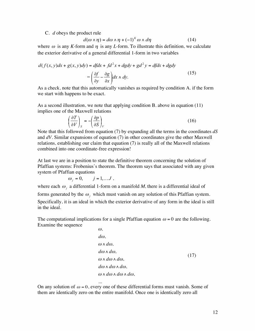
C. d obeys the product rule !"!"!" ddd

K #$+#=# )1()( (14) where ! is any K-form and ! is any L-form. To illustrate this definition, we calculate the exterior derivative of a general differential 1-form in two variables

.=

)),(),(( 22

dydxx

g

y

f

dgdydfdxygddgdyxfddfdxdyyxgdxyxfd

!""#

$%%&

'

(

()

(

(

+=+++=+

(15)

As a check, note that this automatically vanishes as required by condition A. if the form we start with happens to be exact. As a second illustration, we note that applying condition B. above in equation (11) implies one of the Maxwell relations

VS S

p

V

T!"

#$%

&

'

'(=!

"

#$%

&

'

' (16)

Note that this followed from equation (7) by expanding all the terms in the coordinates dS and dV. Similar expansions of equation (7) in other coordinates give the other Maxwell relations, establishing our claim that equation (7) is really all of the Maxwell relations combined into one coordinate-free expression! At last we are in a position to state the definitive theorem concerning the solution of Pfaffian systems: Frobenius’s theorem. The theorem says that associated with any given system of Pfaffian equations Jjj K,1,0 ==! , where each j

! a differential 1-form on a manifold M, there is a differential ideal of forms generated by the j

! which must vanish on any solution of this Pfaffian system. Specifically, it is an ideal in which the exterior derivative of any form in the ideal is still in the ideal. The computational implications for a single Pfaffian equation

!

" = 0 are the following. Examine the sequence

!

",

d",

"#d",

d"#d",

"#d"#d",

d"#d"#d",

"#d"#d"#d",

...

(17)

On any solution of

!

" = 0, every one of these differential forms must vanish. Some of them are identically zero on the entire manifold. Once one is identically zero all

13

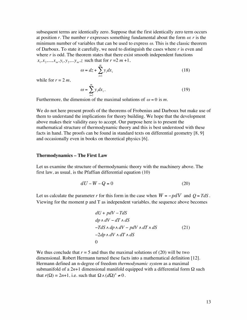
subsequent terms are identically zero. Suppose that the first identically zero term occurs at position r. The number r expresses something fundamental about the form ω: r is the minimum number of variables that can be used to express ω. This is the classic theorem of Darboux. To state it carefully, we need to distinguish the cases where r is even and where r is odd. The theorem states that there exist smooth independent functions

!

x1,x

2,...,xm,y1,y2,...ym,z such that for r =2 m +1,

!

" = dz + yidxii=1

m

# (18)

while for r = 2 m,

!

" = yidxii=1

m

# . (19)

Furthermore, the dimension of the maximal solutions of

!

" = 0 is m. We do not here present proofs of the theorems of Frobenius and Darboux but make use of them to understand the implications for theory building. We hope that the development above makes their validity easy to accept. Our purpose here is to present the mathematical structure of thermodynamic theory and this is best understood with these facts in hand. The proofs can be found in standard texts on differential geometry [8, 9] and occasionally even in books on theoretical physics [6]. Thermodynamics – The First Law Let us examine the structure of thermodynamic theory with the machinery above. The first law, as usual, is the Pfaffian differential equation (10) 0=!! QWdU (20) Let us calculate the parameter r for this form in the case when pdVW != and

!

Q = TdS . Viewing for the moment p and T as independent variables, the sequence above becomes

!

dU + pdV "TdS

dp#dV " dT #dS

"TdS#dp#dV " pdV #dT #dS

"2dp#dV #dT #dS

0

(21)

We thus conclude that r = 5 and thus the maximal solutions of (20) will be two dimensional. Robert Hermann turned these facts into a mathematical definition [12]. Hermann defined an n-degree of freedom thermodynamic system as a maximal submanifold of a 2n+1 dimensional manifold equipped with a differential form Ω such that r(Ω) = 2n+1, i.e. such that

!

"# (d")n$ 0 .

14

A 2n+1 dimensional manifold equipped with a differential form Ω such that

!

"# (d")n$ 0 is called a contact manifold and the form

!

" the contact form. Hermann’s definition can be restated in the following form: a thermodynamic system is a maximal solution of

!

" = 0 , where

!

" is a contact form. The name “contact” has some significance; contact forms arose in mechanics to deal with surfaces rolling on each other [13]. Also in thermodynamics we can interpret the form

!

" as coming from the coexistence of a system with its environment. By Darboux’s theorem, there exist coordinates that make

!

" assume

the canonical form

!

" = dz + yidxii=1

m

# . For simplicity we will carry out our discussion for

the explicit two dimensional case

!

" = dU + pdV #TdS . The parameters (p,T) can be thought of as parameters describing the environment of the system. At equilibrium, the system chooses its state to coexist with this (p,T). In the geometrical picture introduced by Gibbs wherein we view the system as the surface of the function U=U(V,S), the normal vector describing the tangent plane to the surface is (–1, –p, T). As p and T are changed, this tangent plane rolls on the surface in much the same way that mechanical cogs roll on each other. Moving our perspective to the space of the five variables (U,p,V,T,S) reveals the essential nature of this coexistence. The functions (U,p,V,T,S) are by no means the only contact coordinates, i.e., the only coordinates which make

!

" assume the form in equation (18). For example, the classical Legendre transformation always result in contact coordinates

!

" = dH #Vdp#TdS = dG #Vdp + SdT = dF + pdV + SdT (22) where H, G, and F are the enthalpy, the Gibbs free energy, and the Helmholtz free energy. Their usefulness derives from exactly those situations when the environment specifies the coefficients in front of the differentials, i.e., the ‘y’ variables from Darboux’s theorem. This further justifies the view that the ‘y’s describe the environment, the ‘x’s describe the system, and ‘z’ characterizes the contact. Requiring a coordinate change to preserve the appearance of

!

" shown in equation (18) allows many more coordinate changes. These are generalized Legendre transforms [14] and form an infinite dimensional group known as the contact group [15]. Its use to date has been limited by the paucity of exotic environments. Its use has been demonstrated for a system inside a balloon whose pressure and volume obey a definite relationship although neither pressure nor volume are constant. It is potentially useful for biological systems with complex constraints. Besides possible uses of these generalized Legendre transforms, the first law of thermodynamics in the form

!

" = 0 gives a deeper perspective regarding the thermodynamic method. It shows us that this method may be thought of as a theory for “viewing” the inside of black box systems [14]. We manipulate n parameters y in the environment and observe the changes in our black box system as it moves to states of coexistence. In this way we find a thermodynamic theory of the black box. The form

!

" chooses the particular x and z that must go with the y’s describing the system’s surroundings.

15

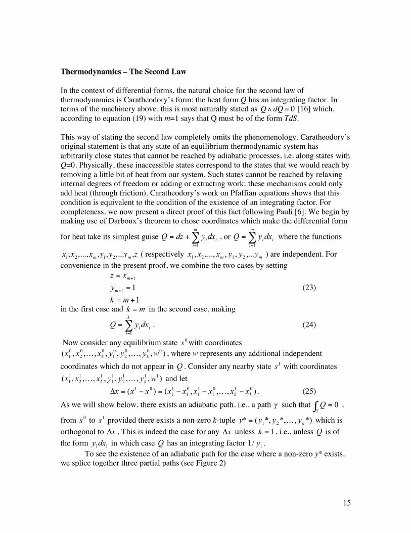
Thermodynamics – The Second Law In the context of differential forms, the natural choice for the second law of thermodynamics is Caratheodory’s form: the heat form Q has an integrating factor. In terms of the machinery above, this is most naturally stated as

!

Q"dQ = 0 [16] which, according to equation (19) with m=1 says that Q must be of the form TdS. This way of stating the second law completely omits the phenomenology. Caratheodory’s original statement is that any state of an equilibrium thermodynamic system has arbitrarily close states that cannot be reached by adiabatic processes, i.e. along states with Q=0. Physically, these inaccessible states correspond to the states that we would reach by removing a little bit of heat from our system. Such states cannot be reached by relaxing internal degrees of freedom or adding or extracting work; these mechanisms could only add heat (through friction). Caratheodory’s work on Pfaffian equations shows that this condition is equivalent to the condition of the existence of an integrating factor. For completeness, we now present a direct proof of this fact following Pauli [6]. We begin by making use of Darboux’s theorem to chose coordinates which make the differential form

for heat take its simplest guise !=

+=m

i

iidxydzQ1

, or !=

=m

i

iidxyQ1

where the functions

!

x1,x

2,...,xm,y1,y2,...ym,z ( respectively

mmyyyxxx ,...,,,...,,

2121 ) are independent. For

convenience in the present proof, we combine the two cases by setting

1

11

1

+=

=

=

+

+

mk

y

xz

m

m

(23)

in the first case and mk = in the second case, making

!=

=k

i

iidxyQ1

. (24)

Now consider any equilibrium state 0s with coordinates

),,,,,,,,( 000

2

0

1

00

2

0

1 wyyyxxx kk KK , where w represents any additional independent coordinates which do not appear in Q . Consider any nearby state 1

s with coordinates ),,,,,,,,( 111

2

1

1

11

2

1

1 wyyyxxx kk KK and let ),,,()( 010

1

1

1

0

1

1

1

01

kkxxxxxxxxx !!!=!=" K . (25)

As we will show below, there exists an adiabatic path, i.e., a path ! such that 0=!" Q ,

from 0s to 1

s provided there exists a non-zero k-tuple *),*,*,(* 21 kyyyy K= which is orthogonal to x! . This is indeed the case for any x! unless 1=k , i.e., unless Q is of the form

11dxy in which case Q has an integrating factor

1/1 y .

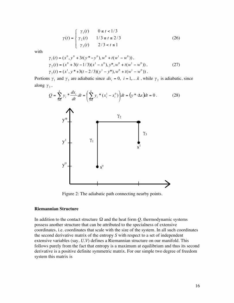
To see the existence of an adiabatic path for the case where a non-zero y* exists, we splice together three partial paths (see Figure 2)

16

!"

!#

$

%<

%%

<%

=

13/2)(

3/23/1)(

3/10)(

)(

3

2

1

tt

tt

tt

t

&

&

&

& (26)

with ))(),*(3,()( 010000

1 wwtwyytyxt !+!+=" , ))(*,),)(3/1(3()( 010010

2 wwtwyxxtxt !+!!+=" , (27) ))(*),)(3/2(3*,()( 01011

3 wwtwyytyxt !+!!+=" . Portions

1! and

3! are adiabatic since kidx

iK,1,0 == , while

2! is adiabatic, since

along 2! ,

( ) 0*)(**1

01

1

=!"=#$

%&'

()== **

==

dtxydtxxydtdt

dxyQ

k

i

iii

k

i

ii . (28)

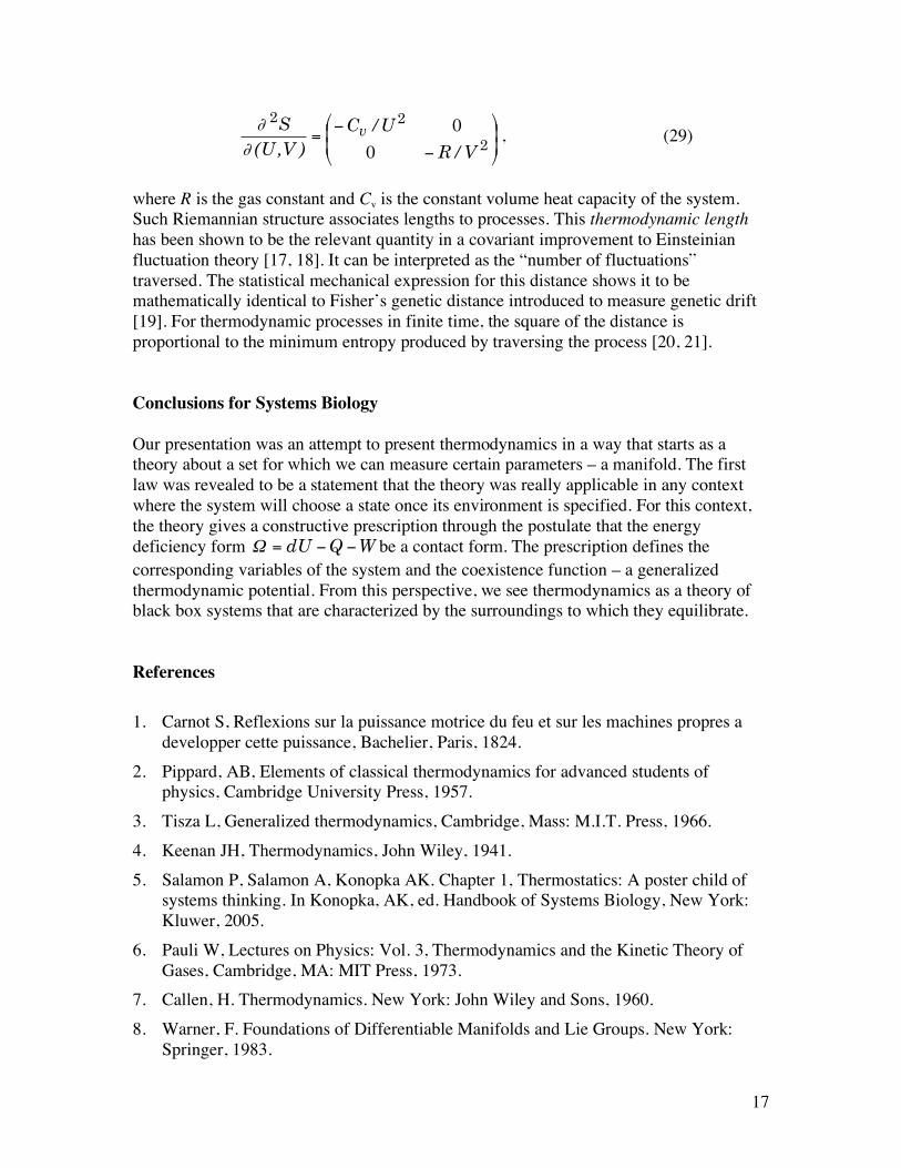
Riemannian Structure In addition to the contact structure

!

" and the heat form Q, thermodynamic systems possess another structure that can be attributed to the specialness of extensive coordinates, i.e. coordinates that scale with the size of the system. In all such coordinates the second derivative matrix of the entropy S with respect to a set of independent extensive variables (say, U,V) defines a Riemannian structure on our manifold. This follows purely from the fact that entropy is a maximum at equilibrium and thus its second derivative is a positive definite symmetric matrix. For our simple two degree of freedom system this matrix is

γ1

γ2

γ3

s0

s1

y0

y*

y1

Figure 2: The adiabatic path connecting nearby points.

17

!!

"

#

$$

%

&

'

'=

2

22

0

0

V/R

U/C

)V,U(

S v

(

( , (29)

where R is the gas constant and Cv is the constant volume heat capacity of the system. Such Riemannian structure associates lengths to processes. This thermodynamic length has been shown to be the relevant quantity in a covariant improvement to Einsteinian fluctuation theory [17, 18]. It can be interpreted as the “number of fluctuations” traversed. The statistical mechanical expression for this distance shows it to be mathematically identical to Fisher’s genetic distance introduced to measure genetic drift [19]. For thermodynamic processes in finite time, the square of the distance is proportional to the minimum entropy produced by traversing the process [20, 21]. Conclusions for Systems Biology Our presentation was an attempt to present thermodynamics in a way that starts as a theory about a set for which we can measure certain parameters – a manifold. The first law was revealed to be a statement that the theory was really applicable in any context where the system will choose a state once its environment is specified. For this context, the theory gives a constructive prescription through the postulate that the energy deficiency form WQdU !!=" be a contact form. The prescription defines the corresponding variables of the system and the coexistence function – a generalized thermodynamic potential. From this perspective, we see thermodynamics as a theory of black box systems that are characterized by the surroundings to which they equilibrate. References 1. Carnot S, Reflexions sur la puissance motrice du feu et sur les machines propres a

developper cette puissance, Bachelier, Paris, 1824. 2. Pippard, AB, Elements of classical thermodynamics for advanced students of

physics, Cambridge University Press, 1957. 3. Tisza L, Generalized thermodynamics, Cambridge, Mass: M.I.T. Press, 1966. 4. Keenan JH, Thermodynamics, John Wiley, 1941. 5. Salamon P, Salamon A, Konopka AK. Chapter 1, Thermostatics: A poster child of

systems thinking. In Konopka, AK, ed. Handbook of Systems Biology, New York: Kluwer, 2005.

6. Pauli W, Lectures on Physics: Vol. 3, Thermodynamics and the Kinetic Theory of Gases, Cambridge, MA: MIT Press, 1973.

7. Callen, H. Thermodynamics. New York: John Wiley and Sons, 1960. 8. Warner, F. Foundations of Differentiable Manifolds and Lie Groups. New York:

Springer, 1983.

18

9. Bishop RL, Goldberg SI, Tensor analysis on manifolds, New York: Dover Publications, 1980.

10. Eisenhart LP, A treatise on the differential geometry of curves and surfaces, Ginn and Company, Boston, 1909.

11. Poincare H, Les methodes nouvelles de la mecanique celeste, Gauthier Villars, Paris (1892)

12. Hermann R. Geometry, Physics, and Systems, New York: M. Dekker, 1973. 13. Ball RS. Treatise on the Theory of Screws, Cambridge, UK: Cambridge UP, 1900. 14. Salamon P. The Thermodynamic Legendre Transformation or How to Observe the

Inside of a Black Box, PhD Thesis, Department of Chemistry, University of Chicago, 1978.

15. Salamon P, Ihrig E, Berry RS, A Group of Coordinate Transformations Preserving the Metric of Weinhold. J. Math. Phys. 1983; 24: 2515.

16. Edelen, D. The College Station lectures on thermodynamics, College Station, TX: Texas A & M University, 1993.

17. Diosi L, Lukacs B, Covariant evolution equation for the thermodynamic fluctuations. Phys. Rev. A, 1985; 31: 3415-3418.

18. Ruppeiner G, Riemannian geometry in thermodynamic fluctuation theory. Rev. Mod. Phys. 1995, 67: 605–659.

19. Salamon P, Nulton JD, Berry RS, Length in Statistical Thermodynamics. J. Chem. Phys. 1985; 82: 2433-2436.

20. Salamon P, Berry RS, Thermodynamic Length and Dissipated Availability. Phys. Rev. Lett. 1983; 51: 1127-1130.

21. Nulton J, Salamon P, Andresen B, Anmin Q, Quasistatic processes as step equilibrations. J. Chem. Phys, 1985; 83: 334-338.