Embed Size (px)
Citation preview
.-- . t. orô
The mathematical analysis of
crossover designs
Sadegh Rezaei, B.Sc (Hons) (Ahwaz University), M.Sc (Tarbiat
Modarres University)
Thesis submitted for the degree of
Doctor of Philosophy
?,n
Stat'ist'ics
at
The Uniuersity of Adela'ide
(Faculty of Mathematicøl and Computer Sciences)
Department of Statistics
November 18, 1997
I
*tr|'

Contents
Contents
List of Tables
List of Figures
Summary
Signed Statement
Acknowledgements
1 Introduction and literature revlew
1.1 Introduction
1.2 Definitions .
1.3 Fields of application
I.4 Background and problems
1.5 Review of previous work on two-treatment designs
1.5.1 Optimality for crossover designs
1.6 Structure of the thesis
2 Models for crossover designs
2.1 Introduction
2.2 The model and information matrices
ll
vlll
xll
xlll
xv
xvt
1
1
,)
3
4
5
I
I
12
t2
ll
13

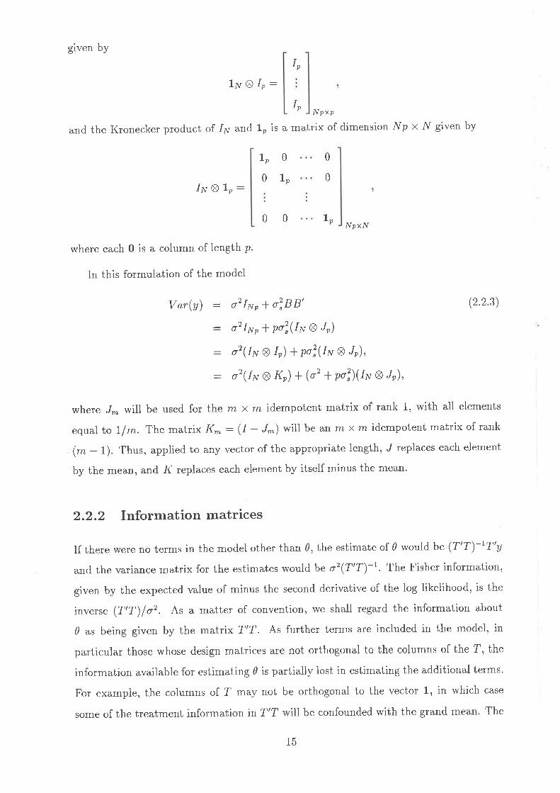
2.2.1. Nlixed linear model
2.2.2 Information matrices
2.3 Estimating the parameters of interest
2.4 Building the model and information matrices using averages
2.4.I Linear model for averages
2.4.2 Variance matrix of the groupxperiod means
2.4.3 Idempotent matrices for strata
2.5 Analysis of variance .
2.6 Analysis based on means
2.6.I The vector of means
2.6.2 Combining information about treatment parameters
2.6.3 SummarY of Chi's Paper
2.7 trqual gïoup sequence analYsis
2.8 Conclusion .
3 Analysis of two-treatment two-period crossover designs
3.1 Introduction
3.2 Two-treatment, two-period crossover design
3.2.1 Analysis of design when ) is present
3.2.2 Treatment information
3.2.3 Analysis of the design when ) is not present
3.2.4 Analysis of design when subject effect is fixed
3.2.5 A comparison of the three cases of 2 x 2 crossover design
3.3 Baseline measurements in the 2 x 2 crossover design
3.3.1 One baseline measurement in the design
3.3.2 Two baseline measurements in the design .
13
15
1,7
18
20
21.
22
22
23
23
26
27
28
30
31
31
32
33
35
JI
38
39
40
4l
45
483.3.3 Conclusion and discussion
lil
3.4 Balaam's design for tlvo treatments
3.4.1 Balaam's design rvhen subject effects are random and unequal
group slzes.
3.5 Tlvo-treatment, three-period crossover design
4 A Bayesian analysis for the general crossover design
4.1 Introduction
4.2 The statistical linear model
4.3 Likelihood and parameter estimation
4.4 Bayesian analysis
4.4.1 Xo is a nonsingular matrix
4.4.2 X6 is a singular covariance matrix
4.5 Choice of prior distribution
4.6 Two-treatment, two-period design
4.6.1 Posterior estimates
49
50
54
67
õ(
59
60
63
63
64
67
69
69
7t
t.)
74
/b
4.7
4.8
4.9
Two-treatment, two-period with one baseline measurement
Two-treatment, two-period with two baseline measurements
Bayesian analysis of Balaam's design
4.10 Three-period designs with two groups
5 Analysis of a two-period crossover design for the comparison of two
active treatments and placebo 78
5.1 Introduction 78
5.2 The linear model
5.3 Treatment information 81
5.4 Combination of the estimates
79
83
5.5 Conclusions
IV
84

6 Cohort designs for two-treatment crossover trials with one baseline
measurement 87
6.1 Introduction.
6.2 Age-period-cohort design
6.3 Building the model for standard and cohort designs
6.4 Standard design
6.4.1 Information matrices and parameter estimates
6.4.2 Analysis of variance for standard design
6.5 Cohort design
6.6 Treatment information
6.6.1 Information matrices or þt:10 * )6 and þz: ro- Ào
6.6.2 Where is the treatment information?
6.7 Combining information
6.7.1 Estimation of (re, Às) in cohort design only
6.7.2 Estimation of (rp,)p) in both designs
6.7.3 Estimates of treatment effect minus baseline
6.8 Limiting estimates in terms of p .
6.8.1 The estimates and covariance matrix when p -+ æ
6.8.2 Estimates and their covariance when p -+ 0
6.9 Conclusion .
7 Block structure of cohort designs
7.t Introduction .
7.2 Cohort design in general
7.3 Analysis of variance
7.4 Fitting periods and cohorts
7.5 James and Wilkinson theorem

7.5.7 Canonical variables
7.6 Expected mean squares of each block structure
7.7 Description of a function cc in S-PLUS to get the result of James and
Wilkinson's theorem
7.7.1 Projector matrices
\23
r25
129
t32
7.8 To get a pattern on p and the Cohort (elim. Periods) contrasts 133
7.9 Conclusions 134
I Treatment structure of cohort designs 135
8.1 Introduction 135
8.2 Treatment structure for cohort and standard designs in general 136
8.3 Projector matrices for cohort and standard designs in general 137
8.4
8.5
8.6
8.7
8.3.i Estimates of parameters and covariance matrix of estimates 139
Treatment information for two-treatment crossover design with two base-
line measurements and a corresponding cohort design i40
8.4.1 Treatment information when the first-order carryover is present 742
8.4.2 Treatment information when carryover effect is not present I44
Treatment information for two-treatment, extra-period crossover design
and its corresponding cohort design with one baseline measurement I45
8.5.1 Treatment information when first-order carryover effect is present I47
8.5.2 Treatment information when the first-order carryover is not present 151
Treatment information for three-treatment and three-period crossover design152
8.6.1 Treatment information when carryover effect is present 153
8.6.2 Treatment information when ca ryover effect is not present 155
Treatment information for two-treatment with one baseline measurement
with more than two cohorts 156
8.7.1 Treatment information when c: 3 and first-order carryover effect
is present
VI
r57

8.8 Conclusion
Appendices
A Some useful concepts from linear algebra
4.1 The Kronecker product .
A.2 Idempotent matrices
r59
161
161
161
r62
r62
t62
t62
164
165
165
167
r67
170
L76
Positive definite quadratic forms and matrices
Contrast and orthogonal contrasts .
ANOVA sum of squares as quadratic forms .
4.6 Summing vectors,, and -E-matnces
B Bayes'theorem
8.1 Normal prior for multinormal sample
C The S-PLUS program for cohort designs
C.l S-PLUS functions
Bibliography
4.3
4.4
A'.5
C.2 Use of S-PLUS functions for Chapter 6
vll

List of Tables
2.1 Layout of the design 13
2.2 Group x period means 19
ANOVA table for standard design, no treatment terms. 22
ANOVA table for standard design, using means, no treatment terms. 26
ANOVA table for standard design, equal size groups, no treatment terms. 29
2.3
)A
2.5
3.1 Notation and layout for the simple crossover design
3.2 Expectation of responses in 2 x 2 crossover design when ) is in the model 33
3.3 Weighted orthogonal matrices for four strata in the design 35
3.4 Estimates of parameters and their variances. 39
3.5 Two-treatment design with one baseline measurement 4l
3.6 Expectation of responses in 2 x 2 crossover design when À is in the model 42
3.7 Weighted orthogonal matrices for four strata in the design 43
3.8 Two-treatment crossover design with two baseline measurements 45
3.9 Weighted orthogonal matrices for four strata in the design 47
3.10 The layout of Balaam's design with the number of subjects in each group. 50
3.11 Expected value of mean in Balaam's design
3.12 Weighted orthogonal matrices for four strata in Balaam's design
3.13 Two-treatment,, three-period crossover design
4.I Layout of general crossover design .
32
50
51
54
58
vlll

4.2
4.3
4.4
4.5
Idempotent matrices of each stratum
Table of idempotent matrices with their ranks
Expected values of responses in two-treatment.l two-period design.
Expected values of responses when treatment B is a standard treatment
59
61
67
67
795.1 Layout of design with two active treatments and placebo
5.2 Expected values of responses in comparison of two active treatments and
placebo. 80
b.3 Idempotent matrices for four strata in the design including placebo. 8i
6.1 Two-treatment three-period crossover design with baseline measurements 91
6.2 Cohort design in two-treatment three-period crossover design with one
baseline measurement .
6.3 Two-treatment three-period crossover design with one baseline measure-
ment repeated as 4 groups of n.
6.4 Treatment effects for the 12 means of observations for two-treatment three-
period crossover design
6.5 Ana,lysis of variance for standard design
6.6 Projector matrices for cohort design for two orders of fitting 101
6.7 Matrices introduced in the table of projector matrices for cohort design 101
6.8 Information matrix in each stratum for both designs 103
92
92
93
97
6.9 Information matrix about Ér and B2 in each stratum for both designs
6.10 Percentage of information in each stratum about ro * )o and rs - )o for
the cohort design 105
6.11 Those strata which contribute to estimate some parameters of interest . 107
6.12 Contrasts for estimating parameters in cohort design 108
6.13 Contrasts for estimating parameters in standard design i08
7.1 ANOVA table for standard design, no treatment terms.
105
IX
i19

7.2 ANOVA table for general cohort design, no treatments term
7.3 Helmert contrasts for Periods
7.4 Helmert contrasts for Cohorts
7.5 Contrasts for three cohorts and three periods
7.6 Canonical correlation coefficients and orthogonal contrasts for two cohorts
and various periods
7.7 Canonical correlation coefficients and orthogonal contrasts for three co-
horts and various periods .
8.1 Projector matrices for general standard design
8.2 Projector matrices for general cohort design
8.3 Two-treatment ctossover design with two baseline measulements
8.4 Cohort design in two-treatment, two-period crossover design with two
120
130
131
t32
I ,J,)
734
138
138
r40
baseline measurements. T4T
8.5 Expected values of two-treatment, two-period crossover with two baseline
measurements when we consider the cohort design or double standard design.141
8.6 Information matrices for standard and cohort designs in two-treatment
design with two baseline measurements, when first-order camyover effect
is present 143
8.7 Orthogonal contrast on Cohort (elim. Periods) I44
8.8 Information matrices for two-treatment, two-period standard and cohort
designs when first-order carryover effect is not present. 145
8.9 Tlvo-treatment, extra-period crossover design with one baseline measurementl46
8.10 Cohort design for two-treatment, extra-period crossover design with one
baseline measurement t46
8.11 trxpected values for design of two-treatment, extra-period crossover trial. 147
8.12 Information matrices for standard and cohort two-treatment, extra-period
designs lvith one baseline measurement. .
X
r49

8.13
8.14
8.15
8.16
Treatment information for both standard and cohort two-treatment, extra-
period design with one baseline when the carryover effect is not present. . 151
Three-treatment, three-period crossover design 152
Cohort design in three-treatment and three-period crossover design 153
Expected values for three-treatment, three-period crossover and its corre-
sponding cohort design 153
8.17 Information matrices for standard and cohort designs for three-treatment,
three-period
8.18 Treatment information for both standard and the cohort designs in three-
treatment, three-period when the carryover effect is not present. 155
8.19 Two-treatment crossover design with one baseline measurement when c:3156
8.20 The 18 means for two-treatment with one baseline measurement when c : 3156
8.21 Information matrices for standard and cohort designs for two-treatment
with a baseline, c: 3 158
8.22 Information or rs and Às in three cases of design . . 159
. 754
XI

List of Figures
lú times variance of (i) direct treatment effect and of (ii) carry-over effect
estimatorfor 2x2 designinterms of p:0,1,2,5,10,20 and q : rtl(nt-ln2). 40
Conditional distribution of carryover effect given direct effect 68
Relation between posterior estimates when Ic :0.2 73
3.1
4.t
4.2
5.1 Standard deviation of î¡ as p changes
6.1 Diagram of cohort design and its main concepts in crossover trial
6.2 The relationship of projector matrices in cohort design
7.1 Full cohort design length cpgn .
7.2 Full cohort design, length cp . .
7.3 Cohort design for three periods in each cohort
99
86
89
118
tzt
130
xll
Summary
The mathematical analysis of crossover designs
Sadegh Rezaer
Department of Statistics
The common theme of this thesis is the theory and application of crossover designs. In
this thesis both classical and Bayesian approaches are considered. The thesis covers three
broad areas.
In the classical approach, the methodology of repeated measurements is used to de-
velop structure and models to describe the properties of crossover designs with different
numbers of periods and unequal numbers of subjects in each group. The common ap-
proach in this part is to look at the information available about treatment parameters
and to see in which strata this treatment information resides. Estimates are obtained
by combining the available treatment information from different strata, in particular,
from the between-subject and within-subject strata. The estimates are equivalent to the
generalised least squares estimates.
To obtain the Bayesian analysis of crossover designs, prior distributions are chosen for
carryover and direct treatment effects to reflect the current state of information about
these parameters and the relationship between them. The assumption made in this
thesis is that since the effect of a treatment dies away over time, we might expect that
the carryover effect in the next period is some proportion, less than 1, of the original
treatment effect. It is assumed that the a priori information is summarised by the fact
that lve expect À to be a proportion k of the treatment effect r, but with uncertainty
described by a variance oSl where afr ìs known and k is some small positive value less
than one. In addition it is supposed that the r has an un-informative uniform prior
xlll

distribution.
Traditional crossover designs, even if baseline measurements are included' still do
not allorv estimation of the difference between the average treatment effect and baseline,
unless one is prepared to make strong assumptions about the period effects, in terms of
their size or likely variance. In the third part of the thesis, an approach is developed in
which some subjects enter the trial with a delayed start. If the situation justifies the twin
assumptions that period effects are related to calendar time (e.g. time of year), and that
there are no effects due to the length of the time in the trial, referred to here as 'age', then
such designs allow the estimation of the average effect of treatment versus baseline. The
designs have similarities to age-period-cohort designs, and they are referred to here as
'cohort designs'. They represent an interesting example of designs with non-orthogonal
block structure.
XIV

Signed Statement
This work contains no material which has been accepted for the award of any other
degree or diploma in any university or other tertiary institution and, to the best of my
knolvledge and belief, contains no material previously published or written by another
person, except where due reference has been made in the text.
I consent to this copy of my thesis, when deposited in the University Library, being '
available for loan and photocopying'
DArE , . .L/.1L-/ .t? 2 7SIGNED:
XV

Acknowledgements
I wolld like to thank my supervisor, Prof. Richard Jarrett, for his support, encourage-
ment and enthusiasm throughout the development of this work. I also thank him for his
accessibility at all hours in considering aspects of the work, and the many hours spent in
discussion and proof-reading.
Many thanks go to Dr Bill Venables due to his assistance relating to computer pro-
grams in particular, S-PLUS and MAPLB enquiries.
I also would iike to acknowledge the financial assistance of the Ministry of Culture
and Higher Education (MCHtr) of Islamic Republic of Iran during the period 26lal92 to
26lI196 in the form of a University of Shahid Chamran Schoiarship.
XVT

Chapter 1
Introduction and literature revle\M
l-.1 Introduction
Clinical trials attempting to compare the efficacy of two treatments often use the two-
treatment two-period crossover design, in which each subject is randomly assigned to
receive both treatments in one of two sequences. This can lead to estimates of the
difference in treatment efficacy that have variances which are less than half of those
provided by the standa¡d parallel design, in which each subject receives, by random
allocation, one treatment only. This reduction of variance results from the elimination
of between-subject variability. Another reason for choosing the crossover design is the
reduced cost of performance of the experiment.
Designs in which experimental units receive more than one treatment application in
the course of the experiment are called crossover designs. Such designs are known by
different names in the literature: changeover designs, or repeated measurement
designs, in some cases. In this design, the experiment is split up into different periods.
Each subject receives one treatment in each period. Usually each subject is observed for
the same number of periods. Designs are composed of several treatment sequences, each
subject being allocated to a sequence at the start of the experiment. It is often assumed
that equal numbers of subjects are allocated to each sequence.
The response variable is often supposed to be continuous. The analysis of crossover
designs when the response is binary has been discussed in the literature by, for example,
Gart (1969), Prescott (1981), Farewell (1985), Jones & Kenward (1987), Kenward &
1

Jones (i9S7b), but little has been written concerning the design of such experiments.
Gart (1969) has given an exact test for comparing matched proportions in the analysis of
binary responses in the crossover designs. Layard & Arvesen (1973) discuss the analysis
of Poisson data in crossover designs, although this seems to be restricted for all practical
purposes to the two-treatment, two-period crossover trial.
As Hedayat & Afsarinejad (1973) pointed out, the need for this design cari be justified
in several ways.
1 Due to budget limitation, the experimenter has to use each subject for several tests
2. In some experiments, the subjects are human beings or animals and often the nature
of the experiment is such that it calls for special training over a long period of time.
Therefore, due to time limitation, one is forced to use each subject for several tests.
3. One of the objectives of the experiment is to find out the effect of different treat-
ments on the same subjects in drug, nutrition or learning experiments.
4. Sometimes the subjects are ra e, therefore the subjects have to be used repeatedly.
The crossover design is a special case of a randomised control trial and has some appeal
to statisticians, medical and psychological researchers. The crossover design allows each
subject to serve as their own control and this, in theory, should reduce the background
level of variation affecting treatment comperisons. Direct evidence moreover., can be
obtained about individual subject preference since each subject receives two or more
different treatments.
In the simple casc known as the two-period two-treatment crossover design or the
2 x 2 design, each subject receives A or B in the first period and the alternative in the
succeeding period. The order in which A and B are given to each subject is randomised.
Ideally, half of the subjects receive the sequence AB and half of the subjects receive
the sequen ce B A. This is so that any trend from first-period to second-period can be
eliminated in the estimate of differences in response. In any particular case, the numbers
in the groups may not be identically equal for a variety of reasons, including drop-out and
the nature of the randomisation which might necessarily be done sequentially as subjects
enter the trial over time.
2

I.2 Definitions
The area of crossover design like any other area of statistics contains certain terms rvhich
are not found or used elsewhere. Terms like "direct effect "and "residual effect"
or "carryover effect" ,, washout period and baseline measurement are the most
commonly used ones. These terms are defined belolv.
1. The effect that a treatment has during the period in which it is applied is referred
to the direct treatment effect.
2. The effect of a treatment that persists into the next treatment period is referred to
as the carryover effect.
3. Sometimes, steps are taken by the experimenter to prevent or make less severe
the occurrence of carryover effects by use of a waiting period, commonly called a
washout period, between applications of treatments.
4. ln some situations, the experimenter takes a measurement from the subject before
a treatment is giver i.: the subject. These measurements are known as baseline
rneasurements.
Many authors have discussed the design and analysis of the two-period and two-treatment
crossover design with and without baseline measurements or using washout period or
using extra treatment periods or extra groups in comparing two treatments and have
addressed the issue of carryover effects. The general conclusion of this work is that the
presence of carryover efiect invalidates the use of this crossover design, and that, unless
carryove effects are negligible, a parallel design should be employed, or,, rf a crossover
design has been used, that the analysis should be based only on first period data.
1.3 Fields of application
Crossover designs have had application over many years in a broad spectrum of research
a eas, including agriculture experiments, Cochran (1939), animal husbandry, Cochran
et al. (1941), bioassay procedures, Finney (1978)) food science, market research, medicine,
pharmacology, psychology. However, among applications in occupational psychology,
ù

Parkes (1982) gives an interesting example where the crossover design occurs naturally.
Various examples of the use of these designs in industry can be found throughout the
literature, for example Raghavarao (1989). An important area rvhere crossover designs
are often used is in clinical trials and the pharmaceutical industry. One particular de-
sign, the trvo-treatment, two-period design has been extensively used and lvidely studied
in the literature. The book by Jones & Kenward (1989) lists more than one hundred
papers that have been written on this subject. But there are still several challenging and
practically useful unsolved problems awaiting solution'
L.4 Background and problems
Despite the advantages mentioned above, the design has fallen somewhat into disrepute
because of the possibility of a carryover effect, or a period-by-treatment interaction. A
term for carryover treatment effect is introduced into the model to allow for the ab-
sence or inadequacy of washout periods. If the effect of treatment does persist into the
period following the period of administration, then a carryover term is inclucled in the
model and the estimates of the direct treatment effect will be based on all the data of
design. For a more detailed discussion of the issues involved, see Abeyasekera & Curnow
(1984). Unfortunately, if such a carryover effect is present, naive estimation of the direct
treatment effect will be potentially completely misleading and this design cannot give
an unbiased estimate of direct treatment effect. The US Food and Drug Administration
suggested that this design should not be used, unless unequivocal external evidence of
the absence of carryover was available. Brown (1930) took a similar unfavourable view
of this particular crossover design. There are many papers that react against this feeling
about crossover in general,, see Healy, in discussion of Lewis (1983), Barker et al. (1982),
Patel (1933) and Willan (1983). Moreover, although it is theoretically possible to test for
a caïryover effect, in most small experiments the test is not at a1l powerful. In addition
as Senn (1988) has argued "the significance tests for a ca ryover effect are a form of
self-delusion" and he agreed that the justification for a crossover design must depend on
medical opinion. In this regard he recommended using a washout period to achieve the
atm
The main purpose of a crossover design has been to devise designs that allow the
4

treatment effect to be estimated within-subject. If the subject effects are assumed to be
fixed, then any estimator of direct treatment effect must be within-subject. Some authors
assume that the subject effects are random; this assumption leads to a betrveen-subject
estimate for direct treatments as well, and this can be combined with the rvithin-subject
estimates, as described by Chi (1991).
1.5 Review of previous work on two-treatment de-
srgns
The analysis of crossover designs has been done in the literature using various methods.
In parametric methods, a linear model is set up with all the parameters of interest and
normal least squares techniques are used to obtain estimates of these parameters or
parameters of interest, thus allowing hypothesis tests to be performed. Despite many
variations of approach there is one point on which authors are in substantial agreement,
namely the desirability of a preliminary check for the presence of carryover effects in the
design. The development of the methods starts from the most elementary technique, given
by Gr\zzle (1965), reviewed recently by Senn (1991), and continues through the various
statistical methods proposed by Balaam (1968), who used four groups to compare just two
treatments. Chassan (1964), Ebbutt (1984), Federer & Atkinson (1964), Fletcher (1987)'
Freeman (1989), Jones & Kenward (1939) consider this design with various features of
analysis to get unbiased estimates for direct treatments. The fully Bayesian methods with
informative prior for the parameter of interest were initiated by Grieve (1985), Grieve
(1e86).
The analysis of this design was given by Grizzle (1965) (with a subsequent correction
it Grizzle (1974)), who focused on the simple two-period, two-treatment crossover design
under the model in which subject effects are random. In this paper, Gizzle (1965)
proposed a mixed model for univariate analysis of crossover design. In his model, the
hypothesis of equal carryover (I1o) effects for two treatments is tested from between-
subject variability and since it is regarded as a preliminary test, a relatively high levei of
significance is used. If /lo is not rejected the data from both periods are used for testing
the hypothesis of equal treatment effects. Otherwise, the use of the data from the first
period alone is justified for treatment comparison, resulting in a loss of information.
5

Based on the restrictions of Grizzle's mixed model, several researchers, e.8. Wallen-
stein & Fisher (1977), have been led to respond to the use of crossover designs. They
generally pointecl out the main disadvantages of this design, that is, (i) the loss of infor-
mation when the carryover is present and (ii) the low power of the preliminary test for
ca ryover, as it is based on between-subject variability, and (iii) the increased chance for
bias in the test for equal direct treatment effects derived from the data of both periods.
Zimmermann & Rahlfs (1978) proposed a bivariate normal model and analysed ctossover
,design using a multivariate analysis of variance approach to the repeated measutements
design. Their approach leads to tests identical to those in Gr\zzle's mixed model ap-
proach. They also proposed a method for testing equal camyover effect and direct effect
simuitaneously.
I(och (\g72) described non-parametric methods of analysis for the case of two-treatment,
two-period crossover designs. He proposed a number of non-parametric procedures for
performing various hypothesis tests in connection with the Grìzz\e (1965) model of
crossover trials. One of the various tests which he used was a rank test for direct treat-
ment effect in the presence of carryover effects. Koch's procedure consists of ranking
the period differences for all subjects in the design and then using the Wilcoxon test for
difierences between the two sequence groups. Cornell (1930) extended Koch's result but
only to a small extent.
Brown (19S0) compares the crossover and parallel group or completely randomised
one.period designs in terms of the number of replicates required to achieve a given power
and concluded that the crossover design can yield great savings in cost if the assumption
of no ca ryover effect is valid, but the design should not be used if this assumption is in
doubt. He also showed that the lack of power of the pretest leads with a relatively high
probability to the non-rejection of the hypothesis of no carryover effects when they exist
and the following analysis of the treatment effect in crossover designs is based on a test
biased by carryover effect.
Hills & Armitage (1979) describe particularly clearly the usual method of analysis
for two period crossover design with one measurement in each period per sub.ject for an
ordinal response. For more than two periods it would appear that these analyses are of
little use.
There a e some papers in the study of crossover design in which baselìne measurements
6
are considered. Hills & Armitage (1979), Armitage & Hills (1982), I(ershner & Federer
(1981) and Federer & Atkinson (196a) all applied the baseline measurements and have
limited their discussion to the tlvo-treatment case only. Patel (1983) proposed to consider
baseline measurements which might be obtained prior to each perìod in a two period
crossover design. He showed that these measurements can be used in a preliminary test
to determine the validity of a test for treatment comparison and also for testing the
hypothesis of equal treatment effects.
Wallenstein (1979) showed that, if baseline observations are available before each
period, the two-period two-treatment crossover design may be used for valid estimation
of direct effect even in the presence of carryover effects, under certain constraints about
period effects.
Kershner & Federer (1981) restricted their attention to only two treatments and
compared the variance of contrasts for many higher-order crossover designs in presence
of a mixed effect due to treatment sequences in the model.
We can find an excellent introduction to crossover designs in the book by Jones &
Kenward (1939). Kenward & Jones (i987a), when they introduced the treatment-by-
period-interaction, said that it is desirable that a check be made for it in the statistical
analysis.
Senn (1991) however completely rejected the significance test for carryover and he
said that despite many variations of approach for analysing the crossover design, there
is one common opinion upon which most authors are in substantial agreement, namely
the desirability of a preliminary check for the presence of carryover effects. He in his
paper has argued that the signifrcance test for carryover effect "is a form of self-delusion
and the justification for a carryover design must be dependent on medical opinion as to
whether the wash-out period can be regarded as achieving its aim."
Chi (1991) has shown that we can recover information on direct and carryover treat-
ment effects from a between-subject analysis as is done in an incomplete block design with
subject as blocks. He proved that by combining the within-subject and between-subject
estimates, we can obtain the generalised least square estimate (GLStr), such that the
GLStr estimation is a weighted combination of the within-subject and between-subject
estimates, where the weight depends on the ratio of the between-subject variance compo-
nent o! to the within- subject variance component o2. Laird et al. (1992) also consider
7

the combination of information from between and within subjects and apply their results
to a number of standard designs, such as those of Balaam (1968) and Koch et al. (1989).
Freeman (1989) considered the usual analysis of tlvo-period, tlvo-treatment crossover
design, that is, a two stage procedure in which (i) the presence of carryover is first
tested and then (ii), according as the preliminary test is or is not significant at some
pre-specified level of probability, we eìther use just data from the first period or use all
the data assuming there is no differential carryover effect. Because the preliminary test
for carryover is highly correlated with the analysis of data from the first period only' he
showed that actual significance levels are higher than the nominal level even rvhen there
is no differential carryover. In order to make inference about the difference in treatment
effects he compared three options:
o Procedure PAR, which uses the simple parallel group design, ignoring the second period
altogether.
o Procedure CROS, which uses the differences between first and second periodsl, but
assumes that no carryover effect is present.
o Procedure TS, that is, two-stage procedure for 2 x 2 crossover design proposed by
Grizzle (i965).
He examined the two-stage procedure in terms of mean square error of point estimate,
confldence intervals and actual significance level of hypothesis tests for the differences
between the effects of the two treatments. He showed that even when no carryover
effect exists, the actual significance level of the two-stage procedure of Grizzle (1965)
is substantially larger than the nominal level. The reason is that the pre-test against
carryover effect is highly correlated with the first period comparison test. Thus the
conditional first period test is biased.
One of the main advantages of the crossover design compared with a simple completely
randomised design is that, for a given precision, the study requires fewer subjects. In
order to keep this essential advantage, Lasserve (1991) determined the optimal design for
crossover design with fixed size of population. He paid special attention to the design
with various numbers of periods for comparing two treatments. Willan & Pater (1986)
and \Millan (19S8) develop approaches based on the assumption regarding the rtlationship
betlveen catryover and direct treatment effects.
Some authors in terms of solving the problems have chosen the Bayesian approach.
8

Sehvyn et a1. (1981) have presented a method of analysis for direct treatment effects
in 2 X 2 crossover design with an equal number of subjects in each sequence and an
un-informative prior on the variance component. The Bayesian approach leads to a
magnitude and precision of the experimental estimate, rather than the classical approach
impliecl by a preliminary test. Grieve (1935) has given a Bayesian analysis based on
the Bayes factor against unequai carryover effects which provide a mixture of the tlvo
moclels corresponding to t'absence of the carryover effect" and "presence of the carryover
efiect", in which the weights are both a functìon of the data and of the likelihood of a
carryover efiect. Grieve (1936) in a recent paper extended the Bayesian approach for
tlvo-period crossover when there are tlvo baseline measurements in the design. In his
paper he cleveloped the study of a two-period crossover for displaying the dependence of
posterior inferences concerning the treatment effect on unavoidable prior beliefs about
the correct model.
1.5.1 Optimality for crossover designs
With the restrictions on the number of periods, p, and the number of treatments, f , in a
crossover design, optimality is defined as finding a design that gives a minimum variance
treatment estimator
Just for two treatments, Laska et al. (1983) pointed out that for any number of periods
exceeding two, we can find optimal designs. They have shown that for even numbers of
periods, balanced uniform designs are optimal and for odd numbers of periods, an extra
period design can be used. These results were obtained as special case by Laska &
Meisner (igS5). Kershner & Federer (1981) calculated the variance of estimators for
direct treatment, carryover and total treatment effects for a number of two treatment
designs, using from two to four periods. The various optimality results pointed out are:
the most efficient three-period design is AB B, B AA and the most efficient four-period
design is AAB 8,, B B AA, AB B A, B AAB.
1-.6 Structure of the thesis
The first main purpose of this thesis is focused on the analysis of two-treatment crossover
and using the cohort design in this trial with one and two baseline measurements.
I

The second main purpose of this thesis is concerned with developing a Bayesian
approach to analysis of two-treatment crossover designs by using an informative Normal
density for the parameters of interest.
Chapter 2 develops a general analysis of crossover designs, with the aim of showing
rvhere the treatment information lies in different strata. The focus is on combining all
information in a1l strata to obtain appropriate estimates and showing that r,he estimate
is equivalent to the generalised least squares estimate. In Chapter 3 lve apply the results
from Chapter 2to the two-treatment, two-period crossover design without and with one
and two baseline measurements, Balaam's design and the two-treatment, three-period
crossover design.
Bayesian analysis of general crossover design with an informative prior density with
full rank and non-full rank variance-covariance matrix for the prior density is dealt with in
Chapter 4 and application of the results are shown in this chapter. For choosing the prior
distribution for the parameters of interest, we assume that since the effect of a treatment
dies away over time, we might expect that the carryover effect in the next period is some
proportion of the original treatment effect. It is assumed that the a priori information
is summarised by the fact that we expect À to be a proportion ,k of the treatment effect
r, where k is a small positive value less than one. In addition it is supposed that the r
has an un-informative uniform prior distribution. Analysis of two-treatment, two-period
design with a placebo is shown in Chapter 5.
In the classical analysis of crossover designs, even if baseline measurements are in-
cluded, we could not estimate the difference between the average treatment effect and
baseline, unless we make strong assumptions about the period effects, in terms of their
size or tikely variance. In Chapter 6 an approach is developed for situa,tions in which
some subjects enter the trial with a delayed start. If the situation justifies the twin as-
sumptions that period effects are related to calendar time (e.g. time of year), and that
there are no effects due to the length of the time in the trial, referred to here as 'age',
then such designs, which are referred to here as cohort designs, enable us to estimate
the average effect of treatment against baseline. We compare the results of the cohort
design with the standard design. This alternative design is like an age-period-cohort
design applied to the crosso\¡er trial with baseline in order to recover information about
average effects of treatment and ca ryover. By making some orthogonal contrasts for two
10

important strata lve get the information on the parameters of interest in each stratum.
This treatment information can then be combined to get estimates of the parameters of
interest for the two designs.
In Chapter 7, the block structure of the experiment is presented for the general class
of cohort designs. We use the work of James & Wilkinson (1971), who provide a way of
looking at the array of means and identifying the contrasts for cohorts after eliminating
the effects of periods, i.e. Cohorts(el. Periods), and their expected mean squa es. For
this purpose \rye need to split the Cohort(el. Periods) stratum into different 1 degree
of freedom contrasts each with a different expected mean square and then to identify
the projector matrix for projecting onto the vector space spanned by the columns of
Cohort(el. Periods). This is done in detail for cohort designs with two and three cohorts.
For these special cases we obtain the analysis of variance tables and by using a function
written in S-PLUS (Venables & Rezaei (1996)) we show their projector matrices and the
expected mean square for each contrast in the various strata.
In Chapter 8 we apply treatments to the non-orthogonal block designs of Chapter 7
and use the results of James and Wilkinson's theorem to estimate the treatment effects
in a cohort design and then compare it to a corresponding standard design. We want
generally to see where the treatment information goes and what treatment information
is available by splitting the observations into the several strata and using the idempotent
matrices. To get the estimates of parameters we combine the estimates of parameters
from those strata in which there is some information about parameters.
11

Chapter 2
Models for crossover designs
2.L Introduction
As we mentioned in Chapter I the crossover design can be considered as a repeated
measurements design, since each subject is used on more than one occasion.
The common way of analysing crossover design is to consider subject effects as fixed
effects. As Chi (1991) pointed out, Milliken & Johnson (1984) considered the subjects
as blocks in an incomplete block design and have given the within-subject analysis with
analysis of the averages across periods for all subjects. Gough (1989) has used the
REML approach to recover between-subject information. Chi (1991) also recovered
between-subject information and has shown that the combination of between-subject
and within-subject information is equivalent to a generalised least squares analysis of
crossover design.
In this chapter the methodology of repeated measurements and combining information
from different strata is used to obtain some information about parameters of interest in
the general crossover design with p periods and l/ subjects. The data can be presented
in a table as shown in Table 2.1. Our aim is to look at the information available about
treatment parameters and to see in which strata this treatment information resides.
We will get the estimates by combining information from the different strata and will
show that the estimate is equivalent to the generalised least squares estimate.
t2

2.2 The model and information matrices
Suppose lve arrange the data in a vector, y, reading in order across the rows' so that
U:(At,...,Urp,,...,Uijr...)ANe)tdenotesthevectorofallobservationsonthe.À/subjects
and p periods, such that g;¡ is an observation on the ith subject and in the jth period' as
shown in Table 2.1. Treatments,, yet to be defined, will then be applied to each subject in
each period. Some treatments may in fact be null treatments, corresponding to baseline
measurements.
Period
1
2
Subject
z
¡\i
I2 J p
yij
Table 2.1: Layout of the design
2.2.L Mixed linear model
The mixed linear model for this general case of the crossover design can be given as
y:pl*Pr+BplT0 Ie, (2.2.r)
13

u'here
v
p
7l
p
is the Np x 1 response vector from all subjects in the
design,
is the grand meanl
is the vector of period effects,
is the vector of subject effects, which can be considered
as random effects, normally distributed and independent
with mean zero and variance o!,
is a vector of fixed effects including direct treatment and
ca ryover effects and in some designs may include group
and second carryover effects,
is an lúp x 1 vector with all elements 1,
is the period design matrix of dimension Np x p,
is the subject design matrix of dimension ly'p x N,
is the treatment design matrix of dimension ly'p x ú'
where ú is the number of treatment parameters in the
design,
is an lúp x I error vector whose elements are assumed
normally distributed and independent with mean zero
and variance 02.
Hence the total number of observations is lfp.
For P and B we can put
P : liv E) Ip (2.2.2)
B : 1¡r81p
where I notes the Kronecker product for which the definition and properties are given
in Appendix A, 1 is the identity matrix, and the subscripts denote the length or size of
the matrices, as appropriate.
For example, the Kronecker product of 1¡¿ and I, is a matrix of dimension Np x p
0
t
P
B
T
€
I4
given by
1¡S1o:I v̂
IpNpxp
and the Kronecker product of {y and 1o is a matrix of dimension Np x l/ given by
Leo 0
/ru8lp:o1o 0
00 1pNpxN
where each 0 is a column of length P
In this formulation of the model
V ar(y) : 62lxn + olBB'
: 62lwn + p"?(Iu I /o)
: o'(Iy A /e) + poSUN I /r),
: o'(tu Ø Kp) * (o' + po?)(Iw Ø Jr),
(2.2.3)
where "/- will be used for the n'¿ x Tn idempotent matrix of rank 1, with all elements
equal to If m. The matrix I{^ : (I - "I-) will be an m x m idempotent matrix of rank
(m - 1). Thus, applied to any vector of the appropriate length, ,I replaces each element
by the mean, and If replaces each element by itself minus the mean.
2.2.2 Information matrices
If there were no terms in the model other than d, the estimate of 0 would be (T'T)-rT'y
and the variance matrix for the estimates would be o2(T'T)-1. The Fisher information,
given by the expected value of minus the second derivative of the log likelihood, is the
inverse (T,T) lo2. As a matter of convention,, we shall regard the information about
9 as being given by the matúx T'7. As further terms are included in the model, in
particular those whose design matrices are not orthogonal to the columns of the T, the
information available for estimating d is partially lost in estimating the additional terms.
For example, the columns of T may not be orthogonal to the vector 1, in which case
some of the treatment information in T'T will be confounded with the grand rnean. The
15
information so confounded is T'J¡¡rT. Then the available treatment information in the
space orthogonal to the grand mean is
Te : T'KT.
The information about the parameters of interest 0 can be thought of as residing in
4 different strata, corresponding to the following orthogonal idempotent matrices:
. Qo -- /¡¡ I Jo for grand mean stratum,
. Qt : /¡¿ I K, for period stratum,
. Qz:I{¡v I Jo f.ot between subject stratum,
. Qs :11¡¡ I K, for subject x period stratum,
where we have defined idempotent matrices and their properties in Appendix A.
Information about d is distributed into these 4 strata as
T'Q¿T (i : 0,1,2,3).
Since Q¿ are orthogonal idempotent matrices, we can split the data into four separate
component" Q ¿y and show the properties of each and the relation between them. For the
grand mean stratum, this component can be written as
QoU: p¿l * (lru Ø Jr)r * ("/¡n Øtr)0 * J¡¡oTî * Jxpe.
As noted before, the information about g here is T'JT and we can see that the single
value obtained for the grand mean estimates
u I (Ltn)lp+ Í'T0)l@P),
with a variance ç"' + n"?) l(¡fp). Then ?'("Iiv I Jr)T is the information about 0 contained
in the grand mean. This is completely confounded with ¡; and hence in the absence of
any knowledge about ¡-1, there is no recoverable information about 0, and for this reasonl
the only treatment information available to us is Tt KT.
In the period stratum, the component is
Qß: (1"ø Kr)o*QtTïtQÉ,
so that the treatment information is T'Q1T' andvar(Qg): o"Qt' we note' however'
that this treatment information is compromised by the presence of the period effects.
The information in Periods is only available if we assume that period differences are not
16
present or that they have some known variance. There are unlikely ever to be enough
periods to estimate the variance of an assumed random effect for periods.
Similarly, in the subject stratum lve have'
Qza : (It¡¿ I Lr)p + QrTï I Qze,
so that the treatment information is T'Q¡T, and Var(QzA) : @' + po?)Qz.
Finally for subject x period stratum we can write
esU:esTï*ese,
so that the treatment information isT'Q3T, andVar(QzU): o2. We note that, since
Q¿Q¡:0 (i I j),the components in different strata are uncorrelated. Further,
T,KT: D T,Q¿T,,i=l
so that the total treatment information is split between these strata, each with its own
precision and 3
Var(y):V :D6nQ,,i=O
so that the weighting for the orthogonal idempotent matrices corresponding to each
stratum is given by
6r: o2 + po?, (2.2.4)
2.3
In the general case \¡¡e can rewrite the mixed linear model in Q.a.l) in the following form
a:T0*t (2.3.1)
where all other terms are absorbed into the covariance matrix of (, so that ( - l/(0, V)
such that V is an N x l/ positive definite variance matrix. In doing this, we assume for
the moment that all other terms, even the period effects, can be represented by random
effects. Then
0: (T'V-tT)-LTtV-ta'
6s: o2
do
ôr
Estirnating the parameters of interest
17

If we can write
V :D6nQn,
lvhere Q¿ is the orthogonal idempotent matrix of ith stratum, then we can rvrite
v-t -Сn'Qn'
and the information about 0 canU" tnolrght of as coming from the diftèrent strata, as
T'Q¿T, and providing separate estimates
0¿: (T'Q¿T)-T'Q¿7.
where {-} notes the generalised inverse of a matrix. To get the overall estimate of 9, we
can combine all information in the strata with appropriate weights (ll6;), and hence we
can obtain the following estimate for parameters of interest
0 (Ð ¿,'r' 7nr)- D õo'T' Q oa (2.3.2)
(Ð ¿,' r' 8,r)- (Ð 6;r r' Q ¿T o ¿)
Var(0): (D 6itTtQiT)-
Care needs to be taken in deciding which parts of the information are included. For
example, we decided that the treatment information T'QsT is not useful. Simiiarly, if
we believe that there a e nonzero period effects, then the information T'Q1T will also
contain period effects and hence will not provide reliable unbiased estimates of 0. Hence,
rve would generally use only i :2,3 in recovering the information. This is equivalent to
allowing ôs, ð1 -+ oo, or regarding ¡-l and ¡' as random effects whose variances approach
The variance of this combined estimate is
zero
2.4 Building the model and information matrices us-
ing averages
In later chapters rve consider designs in lvhich subjects are allocated at random into one
of g groups, where all subjects in the same group get the same treatment regime. Suppose
norv that the /ú subjects are divided into g groups, with n¿ (i : l, 2,. . . ,9) in each group'
18

sirch that N : Ðf=r n¿. The data now needs to be indexed with three subscripts às U¿jt ,
where i refers to the group, 7 refers to the subject rvithin the group, and k refers to the
period. If we write the data values as a single vector in standard order, reading across
the rorvs of the table of data, rve have, analogously to equation (2.2.1),
A : Lr]- * Pr + Bp I T0 + e, (2.4.I)
rvhere y is now a vector of length 1/p. The matrix T can be conveniently partitioned into
a separate matrix for each of the g groups of subjects as
T_
1rr, I Tr
ln, Ø Tz
1- eT",'q - v
where 4 is a p x ú matrix defining the treatment assignment for each subject in group i,
for the p periods and the ú treatment parameters in 0.. We can then consider a reduced
table which contains means for each group and each period. In Table 2.2 we show the
group x period means.
Period
1
2Group
g
t2 p Average on Periods
Utt. An. Utp. Ut
Uzt Uzz. Azp. Uz.
Usr. Us2 U sp. Us
Average on Group A t. U.z U.p a
Table 2.2: Group x period means
The period means here are y.j.:Dr¿y¡¡.|N, and the grand mean is y... - Ð"¿y¿..1N.
To identify where the treatment information resides, we give the following G matrix as
the idempotent matrix which produces a vector Gy, where each value U;¡x in the original
data vector is replaced by its group x period mean y¿.¡,:
Jnt o
oJnz00
Jno
Ç-
0
19
8Ip:wØIp (2.4.2)

Thus, Gy has length Np and contains the means repeated so that in the ith group and
jth period, each mean occurs n¿ times. We note that W is an N x N idempotent matrix.
2.4.L Linear model for averages
If we apply the G matrix in the model in (2.4.1)' then rve have
Ga : Gtp, t GPr * GBþ + GTï + Ge,
where the matrix coefficient of ¡; is
ÇlNn: (W ø1o)(l,vo) : (W A 1o)(1,v810) : (Wlr,') S(10) : (1,v) 8(1r) :lryp,
because W is a diagonal matrix with the idempotent matrices as elements on diagonal.
Similarly, for the coefficient of n, we can write
GP : (W Ø/o)(1r I 1o) : (Wt¡v) Ø Ip : lrv I Ip.
Furthermore.'
GB : (W Ø h)QN I 1o) : (W I 1r) (2.4.3)
Let p : (8,r,. . . , p,), be the vector of subject effects, where B¿ is a vector of length
n¿(i:1,. . .,,g). Then for the subject effect we can define
0i : *r'^,þn,where Bi is a scalar, the average of the elements of 0¿. It follows that
GBp : (W ØtòP
Jn. Øle o o
0 JnrØLp 0
Jnn Ø to þn
0'
0,
0
(J",1t) Ø L,
(J",pz) Ø Le
þiL^, Ø L,
þiL"" Ø lp
0
0
(J"ops) Ø le 0[l"n Ø t,1 L",o
08lp
p
pi1
1
n2
00
nl
20
11ng ng p;
B* þ*,
say, where B* : diag(fiL^r,...,fiLnn) 81o.For the treatment coefficient matrix T we
have
Jn, Ø Ip
0
0
Jn, Ø Ip
1', I Tr
Ln, Ø Tz
0
0GT (2.4.4)
(2.4.5)
(2.4.6)
(2.4.7)
(2.4.8)
Lnn Ø Tn
Then the mixed linear model for this purpose can be given by
Gy : þLNp* (lru Ø Ip)n + B*P* + T0 + €"
where e* : Ge.
2,4.2 Variance matrix of the groupxperiod means
The variance matrix of B* B* can be given,, using 2.4.3, by
Var(B*B\ : o2"GBB'G'
: "3(W Ørr)(W S r;)
: p"?(W a /o)
and the variance matrix for e* can be expressed as
V ar(e*) : o2GG' : o2G : oz(W A /o)
Then the variance-covariance of Gy is
Var(Gy) : o'(Wa1o) tpo?(WØJr)
: o"(w Ø Kr) * (o, + po:)(W Ø Jò.
Jnn Ø I,0
T
(2.4.e)
Since Gg provides the vector of group x period means, the matrix (I - G) is the idempo-
tent matrix which projects onto the space orthogonal to this. From (2'4.4), we note that
(I - G)T: 0 and hence that this space has no treatment information, so all treatment
information is in Gy.
27
2.4.3 ldempotent matrices for strata
The information about parameters of interest d can now be thought of as residing in 6
different strata, corresponding to the follorving orthogonal idempotent matrices:
. Qo : /ru I Jo fot Grand mean stratum,
. Q, : /ru I K, for Periods stratum'
. Qz: (W - 4v) I J, for Groups stratum,
. Qs : (W - "I¡v) I I{, for Group x Period stratum,
. Qs: U -W) I "/, for Subject within Groups stratum,
t Q5 : U - W) @ 1lo for Period x (Subject within Groups) stratum'
Now for the analysis of the model lve will consider these 6 idempotent matrices' noting
that in the last two strata, that is, in Qa and Q5, there is no treatment information.
2.5 Analysis of variance
In the previous section some general structure \ryas provided for the general crossover
design. Now in this section we will provide the analysis of variance table for this de-
sign, which simply identifies the components in the block structure and ignores, for the
moment, the treatment structure.
Source Idempotent matrix d.f EMS
GM JxØJp 1
Period JxØKp p-l o2
Group (w-Jp)ØJ, s-I o' + pr?
Group x Period (w-J¡t)ØK, (g-txp-t) o t
Subject within Group (r-w)ØJ.p N-s o' + po?
Period x (subjects within Group ) (r-w)ØKe (¡r-g)(p-t) o2
Total Np
Table 2.3: ANOVA table for standard design, no treatment terms
The data vector y of length lúp, written in standard order, can be partitioned into
various components, corresponding to the terms that can be identified in the linear model
in (2.4.1), and the expected mean squares determined. The general ANOVA for this
22
design is shown in Table 2.3. We note again that the last two strata contain no treatment
information because T''{U -W)ØA}f :0, rvhere A: J ot A: K'
2.6 Analysis based on means
It will be convenient to work lvith the table of group x period means' shown in Table 2.2.
An analysis of this table will give the first four rows of the Table 2.3' but we need to see
how the sums of squa es should be determined from the vector g* of means.
2.6.L The vector of means
To arrange the data in a vector say, g* in terms of averages, the vector y should be
pre-multiplied by a matrix, G", of dimension gp x Np. This matrix is similar to G except
that it does not have repeated rows. Thus the G* matrix can be given as
hL'n,0
0
Ø Ip: (W. Ø h), (2.6.1)1'n"1
n2
0
0L7
0 ùt',0
so that the G* matrix produces the means in a vector y* of length gp and contains just
the means so that, in the ith group and jth period, each mean occurs once. We want to
reproduce the analysis of variance using y*, but with just grand mean,' period, group and
groupxperiod strata. Now in terms of G* we can write
A -<.4
In multiplying the model (2.4.I) by G*, we have
ç"lyn: (W* A 1o)(1¡v A 1r) : ls I Lr: lsp,
G* P : (W- Ø10)(1r I 1r) : (le I 1e),
G*B: (W"8Ir)(I¡u 8lp) :(W* 810).
and
23
G*T
1
nl 1 0
nI
0
ØIp
18nt ØTz
18 r,1
0
0
1
ng
o
0
1 1
fit'ø t, 0
0
0
0 fit'Ø t,18nL ØTz
L,ØIP 1s?n
Tt
T2
Then the mixed linear model for the analysis with means can be expressed as
y* : pLsp* (1, Ø Iòn + (W. Øt)þ + T*0 * G*e, (2.6.2)
such that
V ar(y") : Var(G"e)*Var(G.BB)
: or(w* Ø lr)(w.'a Ie) + "?(w. ØLr)(w*'s t;)
: o2çw*w*'a 1o) * po2,(w.w*' Ø Jo)
: oz1¡-t a 1o) + po"'(N-t Ø Jo)
: ozl¡-t I Ko) + (ot + pø3XN-t I /o)
where
00 ng
Ts
TLy
0 rù2
0
na0
0
0N : (I4l.W*,)-t :
0
We now take each term in Table 2.3 and write it in terms of y* rather then y. All Qis
can be written in the fonnW Ø A, J SAor I Ø A, where A-- J, or A:110. Thus, the
24
sum of squares of W I A is
and, since for W we can lvrite
#t,,0
S Sw.t a*'w Ø A)a*
0
1
I00
In2
0
0ng
0
0 0
0
Tt'¡ n1L,N, 0
0
Ing1ng
iL*, 0 rL2
0 ng lno 0
Tù1 0
w*l0 Tù2
W* : W"'*W*,
0
we can write
SSw¿, : y'(W*'S 1)(N Ø A)(W. ø I)y
: y.'(N g A)y*.
Thus, for A : Jp arrd A: Kp, the sum of squares are
SSwt : y.'(N8J)y*,
SSwp: : y.'(N8 K)y".
Similarly, the sum of squares for the grand mean and periods can be given as
SSt¿, : y'(JØA)y,
where A is replaced by J, and 11r,, respectively.
To get the above sum of squares in terms of U*, the vector of means, we note that
I4l.Nle : 1N, so that
JN : ft"t;1
= Fl4l'.'Nle1;Nl,Ír-
and lve can write1
SSts : ¡u'lw-'A 1)(N1N1'rN ø A)(W. Ø I)y
I *tts: ¡u-'(Nrr'N I A)y..
n2W
I
0
0
ns
25
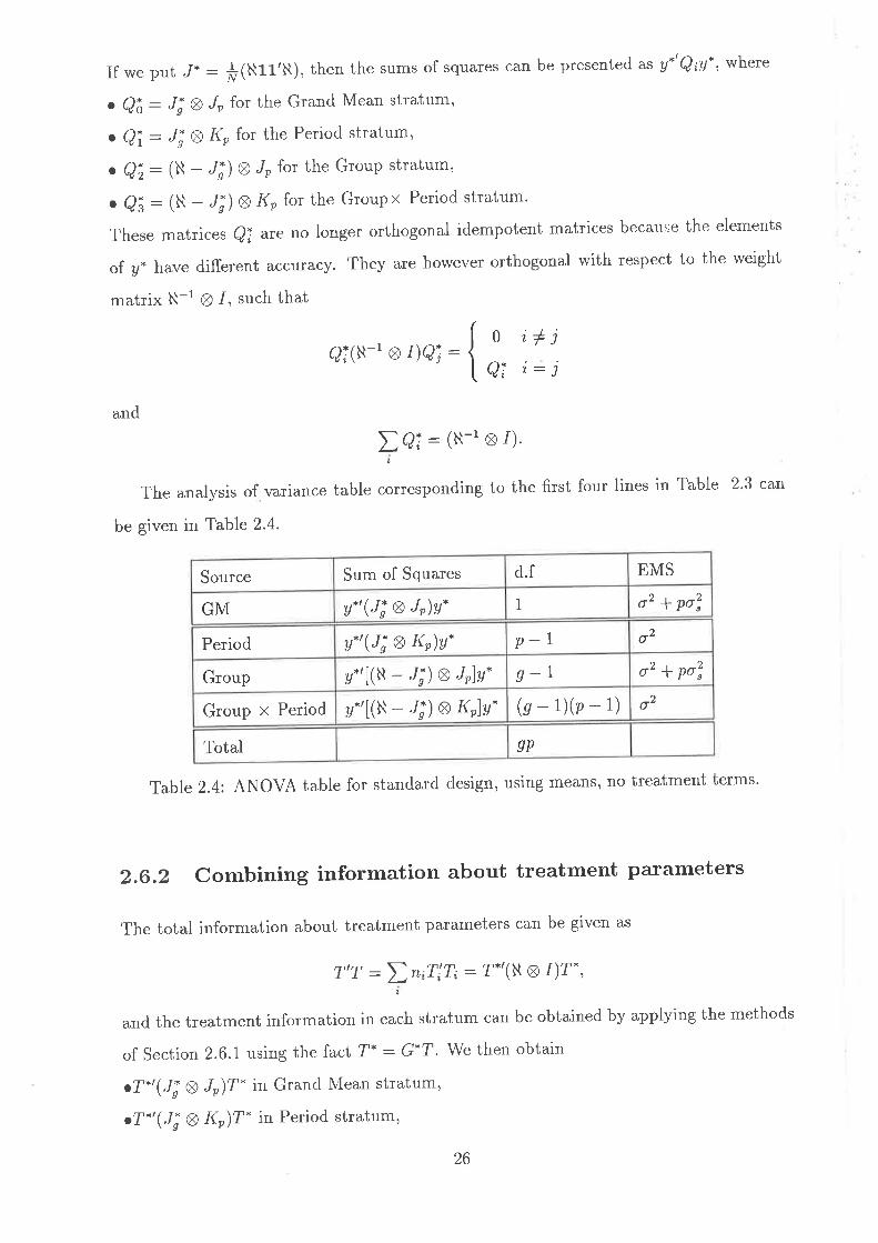
If we put "/.: #(N11'N), then the sums of squares can be presented as Y*'Q¿y", whete
. Qå: ü Ø Je for the Grand Mean stratum,
. Qî: J; Ø I{p for the Period stratum,
. Q;: (N - 4) E ,Io for the GrouP stratum,
. Qä: (N - 4) Ø I{p for the Groupx Period stratum'
These matrices Qi are no longer orthogonal idempotent matrices because the elements
of y* have different accuracy. They are however orthogonal with respect to the lveight
matrix N-1 81, such that
gi(N-' ø r)Qi:
and
\ai: 1N-1 ø 1)'
The analysis of variance table corresponding to the first four lines in Table 2'3 can
be given in Table 2.4.
Source Sum of Squares d.f EMS
GM v*(4 Ø Jòv" I o' + po?
Period v"'(4 Ø Kr)a" p-l o2
Group y.,[(N -¡;)ØJr]y. s-I o2 + po!
Group x Period y.'[(N-JÐØKr]a* (g-tXp-t) o
Total gp
Table 2.4: ANOVA table for standard design, using means' no treatment terms'
2.6.2 combining information about treatment parameters
The total information about treatment parameters can be given as
T'T :ln¿TiT¿: T*'(N 611)T.,
and the treatment information in each stratum can be obtained by applying the methods
of Section 2.6.1 using the fact T" -- G"T' We then obtain
cT"'(Q Ø Jr)T* in Grand Mean stratum,
oT.t($ Ø I{òT. in Period stratum,
0
ai
i+ji:j
26

o?./[(N - JÐ Ø Jr]T" in Group stratum,
oT.'f(N - JÐ Ø I{elT* in GroupxPeriod stratum.
As mentioned before there is no treatment information in the last trvo strata in Table 2.3.
Nolv the estimation of treatment parameters in Grand mean' Period, Group and Group
x Period strata respectively can be given as
0¿ : (7"' QîT-)-T-' Qîy*, (2.6.3)
and the overall estimate of 0 can be obtained by combining the information from those
strata which have useful treatment information, then
á : (D 6iLr.'gîT.)-(Ð 6;tT.'Q;T.o¿), (2.6.4)
and the covariance matrix of this estimate can be given by
V ar(0) : (t 6i rT.' QiT.)- (2.6.5 )
If we regard ¡l and ¡' as fixed effects then the information in the Grand Mean and the
Period strata give one observation or mean for each of the unknown parameters in p and
n-. Hence, unless we know something about the values or distributions of ¡l and n, the
strata represented by the Grand Mean and the Periods provide no accessible information
about the treatment parameters d. We therefore only recover information from Qi and
Q$ with weights óz and ôs.
2.6.3 Summary of Chi's PaPer
Chi (1991) in his paper formalises the between- and within-subject analr'sis for a general
crossover design and shows that the combined estimates are equivalent to the gener-
alised least squares estimates. He defines the following mixed linear model for a general
crossover design
u:T0¡BBIe.,
where g is the vector of effects of parameters of interest includes the period eflect n' and
B is the vector of subject effects. He obtains the following within-subject estìmate of 0,
considering þ in the mixed linear model as fixed effects:
0, : 1r',¡I - B(B' B)-' g'lr\-r'll - B(B' B)-' B'ly.
27

For the estimate of variance o2 he obtains
ã2 : a'lI - B(B', B)-' n',l@ - T0')ll|iD- 1)(1v - 1) - 2(L - t)1,
with B : (8, B)-r B'(A - Tá3) rvhere lV is the total number of subjects in the design and
tr is the number of direct treatments. The covariance matrix of 0s is given as
i,, : "r1f'll - B(B'B)-r B'lTj-.
For the betlveen-subject analysis, he assumes that the subject effects,, B. formed a
random vector distributed as l/(0, ø11). Then the covariance structure for Y is:
Ð:Var(y1 -- olna'+ o2I,
and he obtains the between subject estimate of d as
e, : {r'a(B'B)-t B'r\- {r'a@'B)-r B'a} .
Chi then defines o!: o!l o2lp, and obtains the following estimate
i7:12'z - z'Qor)l(N - ¿.),
where Z: B(B'B)-'B'y,Q: B(B'B)-IB'7, and.L* is therank of Q. The covariance
matrix of gz is
i,2 : pã2ulT'B(B'B)- B'T)-t.
Finally he combines the two estimators of d and got the following generalised least
squares estimators for 0
â : (i; + r;)-'1r;4, + iio.): (T,r-17;-tT'Ð-, y,
where, i: a3An,¡ irI and âl : ;î - or¡p. U"also shows that the combination of the
two estimates of 0 is equivalent to generalised least squares.
2.7 Equal group sequence analYsis
If rve assume that n1 - 'rL2 : "' : Nlg : n, that is, if we assume that the number
of subjects is equally allocated to each group, then the analysis of crossover designs
simplifies. The linear mixed model for the means can be expressed as
y* : p\sp* (ln Ø lr)r + (Ie a lò0* +T*0 + (Ie a Ir),*.' (2'7'l)
28

where €* : G*€ has elements rvhich are l/(0, o'lr), and B* has elements which are
N(0,o! ln). Then we have
V ar(y-)
The Fisher information available in the space orthogonal to the grand mean is
"lriru¿and the data vector distributes into the following strata
.Qö: nJn Ø J, for Grand Mean stratum,,
.Qi: nJn Ø Ko for Period stratum,
.Qi: nKs Ø Jo for GrouP stratum,
.8ä : nl{s Ø K, for Group x Period stratum,
which are orthogonal with respect to the weight matrix (fI) and applied to the vector
of means y*, and
oQa: Kn Ø Is Ø Je for Subject within Group stratum,
.Qs: Kn Ø Is Ø I{p for Period x (Subject within Group) stratum',
which are applied to the data vector y. Then the ANOVA table for this case of design is
shown in Table 2.5.
Source Sum of Squares d.f BMS
GM na*'(Js Ø Jr)a. 1
Period na*'(Js Ø Kr)a* p-l o2
Group na*'(Kn Ø Jr)y" g-l o' + po?
Group x Period nU*'(Kn Ø l{r)y. (g-t)(p-t) o2
Subject within Group a'(K,Ø InØ Jr)y s(" - r) o' + po?
Period x (subjects within GrouP ) a'(I{,Ø InØ Ko)y s(n- tXp- t) o2
Total ngp
Table 2.5: ANOVA table for standard design, equal size groups, no treatment terms.
The treatment information in the ith stratum is the T*'QiT*, and the estimates and their
covariance matrices are as given in Section 2.6.2.
toþJ
: Varl(In 61 1r)..] -f Varl(In A 1r)É.]õ2 no?: î(,,I /e) + ";(ts Ø Jr)
: "l(,16, Ilr) * o2 +-po? (rs Ø Jò,
n"n

2.8 Conclusion
This chapter provides a framework for the analysis of design in which multiple mea-
surements are made on each subject and the variance structure is modelled by random
subject effects and random measurement errors at each period. Treatment regimes are
applied to groups of subjects, possibly with unequal numbers in each group. In the next
chapter, we will apply these methods to some particular designs.
30

Chapter 3
Analysis of two-treatment
two-period crossover designs
3.1 Introduction
This chapter is concerned with two-treatment,, two-period crossover design, in which each
of several groups of subjects receive a different sequence of treatments. In clinical trials
to compare the effects of several treatments, large between- subject variability often
reduces efñciency. To avoid that problem, tesorting to crossover designs has become
popular since they use each experimental subject repeatedly, and tests of treatment and
ca ryover effects can often be performed using within subject variation leading to more
powerful analysis.
In this chapter, we will analyse various aspects of two-treatment, two-period crossover
designs, and have a look at some modifications such as Balaam designs and the use of
baseline measurements, which give us new information about parameters in the model
and resolve the difficulty which we face in the simple 2 x 2 crossover design.
The simplest design is the one known as the 2x2 design. In this design' subjects
are divided into two groups at random. One group receives treatment A followed by
treatment B, and the other group receives the treatments in the reverse order. We will
analyse this design in Section 3.2 just to see the application of Chapter 2 to a weil-
known situation rvhich is analysed by Jones & Kenrvard (1989). In Section 3.3 we will
consider this clesign with one and two baseline measurements. The Balaam design will
31

be considered in Section 8.4 and in Section 3.5 we will give a modification which shows
the optimum design to solve some problems in the 2 x 2 crossover design'
g.2 Two-treatment, two-period crossover design
Suppose we have the 2 x 2 crossover design with two sequences of treatments ,48 and
BA. One measurement or observation is obtained per subject per period in the stan-
dard crossover design, although this measurement might itself be an average of several
measurements of responses taken during the period. Table 3.1 shows the layout for the
data.
Group Subject Period 1 Period 2
Treatment
A B
1
þ,,
0tn,
Uttt
Ultn,
Utzt
At2nt
Treatment
B A
2
þrt
þn"
Azn
Aztn2
Azzt
Azzr2
Table 3.1: Notation and layout for the simple crossover design
The subjects are divided into two groups of sizes n1 and ??2 such that the n1 subjects in
group 1 receive the treatments in the order AB and the n2 subjects in group 2 receive the
treatments in the order BA. Follolving the method in Chapter 2, we assume that Y¿¡¡ is a
random variable lvith the observed value U¿:¿ which follows the mixed linear model given
in (2.2.1). Thus, for the two-treatment, two-period crossover design the model terms for
,4th subject in group 1 would be:
Uttt : p' * þ* t rr * rr I erk, (3'2'1)
Urzt : p'* 7tnIrz*rzI ÀtI etzt.
32

and for group 2 lhey rvould be:
Uzt* p'Iþzn*nrtrzlê2ft.,
¡t * 0z* * ¡rz I rt * Àz I ezz¡.
(3.2.2)
We assume that the subject effects, B¿¡ are random variables from a Normal distribution
rvith mean zero and variance o2, and the errors' e¿¡¡ ale i.i.d random variable from N(0,
or). We also assume that the subject effects and errors are independent. In other
words, we consider o2 as the variance within subjects and ø"2 as the variance between
subjects. We clefine N : nr ! n2 as the total of subjects in the design. In order to
make the parameter values unique, we introduce the following constraints on treatment
parameters:
Ty : -72: T¡
)r : -Àz:À.
(3.2.3)
This section is dir ided into three parts. The 2 x 2 design is considered when À is present
and when it is not present with the subject effect as a random effect. We then discuss
the case with ) in the model and the subject effect as a fixed effect.
3.2.L Analysis of design when À is present
With the constraints in (3.2.3), the expectations of responses in this case can be written
in Table 3.2
Period
Group I
2
1 2
p1'rt*r p,Irz-,¡-+)
þltt-r p,Inz*r-À
Table 3.2: Expectation of responses in 2 x 2 crossover design when ) is in the model
As in Section 2.6, we can examine the treatment information and obtain treatment es-
timates by looking at the vector of means y*. This can be written in matrix notation
Uzzt
,1,)
AS
Utt.
Utz.
Azt.
Azz.
0
1
0
1
0
0
iI
1
1
0
0
1
0
I
0
1
0
1
1
I
I
10pi
p;+
1
-1
-lI
€tr.
€tz.
€zt.
€zz.
(3.2.4)
(3.2.7)
(3.2.8)
tl+l;;1
+ i;1.
where the dot notation in the formulas denotes averages and each mean is lormed by
averaging over the subjects in that group and that period. With the matrix notation of
Chapter 2, we can write out the above mixed linear model as
a* : lrLn * (1, Ø lr)n + B* P* ¡ T*0 ¡ e", (3.2.5)
where y* and 0 are known as data vector and treatment parameters respectively and
B* :W" Ø 10, where
W*: #r'n,0
The covariance matrix of Y* can be obtained by
Var(y.): o'(N-t 6 Kz) * (o'+ 2d3)(N-1 6 Jz) (3.2.6)
where
0
I tlnltn2
N : (14l'.IV*')-t :rL1 0
0nz
n TLTTIZ
By referring to Chapter 2 and incorporating random subject effects, \¡r'e can get the
information matrices about d in the four strata which we introduced in Chapter 2. Since
we reduced the responses to means of observations over the subjects in each groups and
period, we can put
rlJ;: i(Nt1'N) : - TLtTl2 n2,
21
Table 3.3 then shows the relevant projector matrices, which are orthogonal with respect
to the weight matrix N-l I 12, for the four strata identified in Table 2.3. Each stratum
corresponds to just one degree of freedom.
34
Matrix
Grand Mean Qó J;ØJ2 1
2N
n2, n2, TL1tz2
n2, lrfl2
TLtTùZ
TItTL2n21
nl
nl
).,
ta
lTLTù2
fttnz
TLITLZ
TL LTIZ
n
n
Period Qi Ji Ø I{, 1
2N
,,,
-nlTLTTLZ
- TLt TL2
-nl TùtTtz
nl -rùtTlz
-TùtTLz
Tùt'lTZ
n2,
-n"
nl
n2,
-TltTùZ
Tl tTlZ
Group Q; (N-/i)s/, ntn22N
I
i
-1
-1
I
1
1
1
-1
-11
1
1
1
I
1
Group x Period Qä (N-/;) ØKz
1
-1
-11
I
1
1
1
1
1
1
1
1
-1nl n22N
1
I
Table 3.3: Weighted orthogonal matrices for four strata in the design
3.2.2 Treatment information
This separates into a component in each of the three strata, given by
Now, to get the information about treatment parameters $re consider the treatment
information excluding Grand Mean stratum. This is given by
r.'(N81- qilr.-¡i I 4 _21 uS=it tlul_r ,l*TLo rj
12
2N
4-2T* QiT- (3.2.e)
T*,4nyn2
2N
Tl2
2N
q
[:
I
4nt
g;r. 0
1
1
214 2
T-,QäT- :
35
where .^ú : ??r I nz, and I - Tt1 n2. We note that the rank of each of these matrices
is 1. In particular., T-'QiT*(i:1,3) contains information only about (2, - À) and no
information about (r*2À), while T.'8;T* contains information only about À. [f rz1 : Tt2:
there is no information about treatment inT*'QiT*.
We will ignore, as discussed earlier, the information in Çi, the Period stratum. The
estimates of d in the other strata can then be obtained as
1
02 QO Q;T\_T*,Q;Y* n@n. + an.) - @n. -l vzz.)
0 0
t, Az
0": (r,8är-)-r*,Qäy*: å [ ,I,,,-_n),,:,rr*(r;, n:_r]] :
*4,r, -d,2.) [ :, ]
where dt. : ytt. - Ytz. and dz. : Azt. - Uzz..
Thus, á2 provides an estim",":t ) only,
întt"rr:,o.."t:"t an estimateof (2r - ))' since
lz -t I '. :
,(dr - dr.),
and this can be shown to have expected value (2r-)). On the other t und, I IL
so that no information is available for the parameter (z + 2)) in this stratum
In the câ,s€ ?-ù1 I nr, there is information about (2, - )) in the Period stratum, but
this is not recoverable unless ì¡/e are willing to assume that either there is no period effect
or that the period effect is random with a known variance. It can be seen from 3.2.9 that
the information about (2r - )) is split between the Period stratum and the Group x
Period stratum in the ratio 12 : (4np2), and hence that the proportion of the information
lost into Periods is t2f N2: (1 - 2q)2,where q: ft. Clearly, there is no information loss
to Periods when rlt : rL2.
The variance matrices for parameter estimates are
var(02): (o2 +2o?)(7.'8;T-)- : ttt(2'?+zo?)l o t I2n1n2 lo tl
var(03): .2(T*'QäT-)- : ##l : ilL' ^tThe estimates can then be combined using (2.6.4) to give
Q;rr-'q;r* + ótt?*'air")- @;rT-'Q;T*9, * 6;tT-'q|T"0r¡
,f ," 0
l;l36
1
tAn. - Azt.
-\'¿\at.. - az..)
r*p I+2pr -t 2p z(t + 2e)
(3.2.10)
(3.2.11)
(3.2.12)
and' if p : o? lo2, then the covariance matrix for the combined estimates is
( n+*,r*'Q;r* * jr-'qâ?.)-'var{ [;],
No2
4n1n2
we see that an unbiased estimator of r can be obtained as
i : (at. - yzt,) l2'
that is, â is based only on the first period data when À is present in the model. In
other words, if ) is in the model then the estimate of r is based on between-subject
information and is the estimator we would have obtained if the trial has been designed
as a parallel-group study in only one period'
To test the null hypothesis that r:0 when À is in the model, Jones & Kenward
(1989), p. 28, recommend using a two-sample t-test, estimating o2 I o? using only the
first period data. This is different from the estimated variances which would be obtained
by Chi (1991) who proposes estimating both ø2 and ø1, separately' from the full data
set' by equating the mean squares for 8¿ and Q5 to their expectation in Section2'6'
3.2.9 Analysis of the design when À is not present
A further stage of course is that if we do have not a carry-over effect in otrr model then
to get an unbiased estimator of z, we can write
T*:
T",QiT*
T*,8;T"
T*,9äT*
1 -1 -1 1
Then the treatment information in the three strata of interest can be given by
Ðnùf
212
N0
8n1n2
N
and since we have decided not to use the information in the Period stratum the estimate
of z just comes from the GroupxPeriod stratum,' namely
i : (Ytt. - an. - azt. I Yrr.) la
Now we have an unbiased estimator of r based on rvithin-subjects information, and
V ar(î\ : -^[-.o2.8n1n2
We note again that if nt # nzwe lose a proportion (1 - Zq)' of the treatment infor-
mation into the Period stratum. As noted by other authors, the assumption that À : 0
leads to higher precision for the treatment estimate. The efficiency of estimating r with
À in the model compared to estimating r without À in the model is the inverse ratio of
the two variances, namelYNo2 4n1n2
8"t"r^ No,11 ¡¿'which is 50% when p:0, that is there are no between-subject differences, and less the
50%for p>0.
3.2.4 Analysis of design when subject effect is fixed
Our model has subject effects random. This enables us to recover information from
differences between subjects. If the subject effects are fixed, the only information available
is in the differences d¿ : y¿t.-yor.(i : 1, 2) between the two measurements on each subject.
This implies that only the information from Qi and Qi is available. In order to derive a
set of estimates for the parameters of interest, we write the period differences as.
d¡: at.-an.:2¡r*2r-À+er, (3'2'13)
d2 : Yzt.- Yzz.:Ztr -2r* À*(z'
where 7T : ilt - -lt2. By matrix notation
[:; ]:l:l hl.i ; llt;l.l:lwhere Var((¿):2o2ln¿, for i: 1,2. It is clear that
(3.2.r4)
ì:(ú+dz)la
38

with varianceo2var(fr):
srvnlt - 4However we can not distinguish between ¡ and À since (dt- d2) estimates2(2r - )). If
À : 0, (d, - dr)la estimates r rvith a vatiance,
ltar(î\: no' ,.\'/-8Nq(1 -q)'
but as discussed earlier, if ^
+ 0, the only estimate available for r is based on between
subject differences. If the subjects are fixed effects,, we cannot obtain an estimate of r at
all.
3.2,6 A comparison of the three cases of 2 x 2 crossover design
In Table 3.4 we give the results of the analysis of the cÌossover design and have a com-
parison in terms of presence and absence of carryover effect in the model. Let us define
1 n1+n2 t o'
Case
I 2 ,)
Estimator p+0andq+0.5and À is present
p+0andq+0.5
and ) is not present
p:0andq+0.5and À is not present
T T@" Azt.) IlYrr. - an. - Yn.I Yzz.llr 1
ilYrt. - Utz. - Azt.l Uzz.l
À At- - Az None None
Var(î) o2 I
V ar(\) o2 (t+zp)2Nq(1-q) None None
Table 3.4: Estimates of parameters and their variances
We note that the total information about (r, À) is
¡t/2 1
1i
when ?ty : TL2, and hence the best we could hope to do for V ar(î) would be o2 f 2N in the
case rvhere À not in the model. This is achieved iÎ q : j above, but not otherwise. If )
is in the model, the smallest variance achievable for â is o2 (7 I p) I N which is larger by a
39
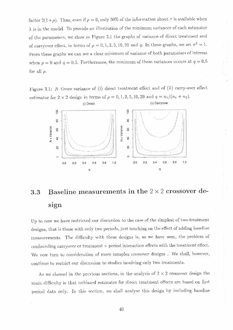
factor 2(I + p). Thus. even if p : 0, only 50% of the information about r is available when
) is in the model. To provide an illustration of the minimum variances of each estimator
of the parameters, we sholv in Figure 3.1 the graphs of variance of direct treatment and
of carryover efiect, in terms of p : 0,1',2,5' 10', 20 and q' In these graphs, we set o2 : f"
From these graphs we can see a clear minimum of variance of both parameters of interest
when p : 0 and q : 0.5. Furthermore, the minimum of these variances occurs at g : Q.5
for all p.
Figure 3.1: N times variance of (i) direct treatment effect and of (ii) carry-over effect
estimator for 2 x 2 design in terms of p - 0,7,2,5, 10,20 and q : ntl(nt -l nz)'
(i) Direct (ii) CarrYover
oo
oó
o@
o+
oAI
I
I
ì
oo
o@
o(o
o{oôt
o
ooc(ú.E(!
xz
\
\
ooc(ú'tr(ú
Xz
0.0 0.2 0.4 0.6 0.8 1.0
q
0.0 0.2 0.4 0.6 0.8 1.0
q
3.3 Baseline measurements in the 2 x 2 crossover de-
srgn
Up to no\¡/ we have restricted our discussion to the case of the simplest of two-treatment
designs, that is those with only two periods, just touching on the effect of adding baseline
measurements. The difficulty with these designs is,, as we have seen, the problem of
confounding carryover or treatment x period interaction effects with the treatment effect.
\Me now turn to consideration of more complex crossover designs . We shall, however,
continue to restrict our discussion to studies involving only two treatments.
As rve showed in the previous sections, in the analysis of 2 x 2 crossover design the
main difficulty is that unbiased estimates for direct treatment effects are based on first
period data only. In this section, we shall analyse this design by including baseline
\
40

measurements lvhich some authors such as Freeman (1989) have recommended. We show
that they can not solve our main difÊculty, but they provide a way to increase the power
of tests against the presence of carryover effect in the model.
Using the baseline in crossover trials has two potential advantages, in that we can
ove come two basic difficulties which we face in the analysis of two-treatment, two-period
crossover design without baseline measurements. The first difficulty is the low power of
the test against of carryover effect. Kenward & Jones (1987a) have shown that one way
to increase the power of this test is to use baseline measurements. The second difficulty,
as Freeman (1939) has suggested, is the over-parameterisation of the design without
baseline measurements. In addition, if there is baseline measurement in the model we
can estimate the average effect of either treatment or carryover, provided lve can make
an assumption about the absence of period effects.
In this work,, we consider baseline measurements in two sections. In the next section we
will take a single baseline measurement before the subjects are given the first treatment.
Then we shall analyse the consequences of the use of baseline measurements before the
subject is given the first treatment as well as the second treatment.
3.3.1 One baseline measurement in the design
In this design there are three periods, in which the first period provides the baseline
measurements. The layout of this design can be shown as in Table 3.5.
Period
gloup
1 2 .)
A B
B A
Table 3.5: Tlvo-treatment design with one baseline measurement
Here the hyphen sign (-) means that there is no treatment implemented in that period.
The model that we apply to the above situation is the same as used in Section 3.2. Now,
by employing the usual constraints on the parameters of interest, the expected values of
observations are given in Table 3.6.
4l
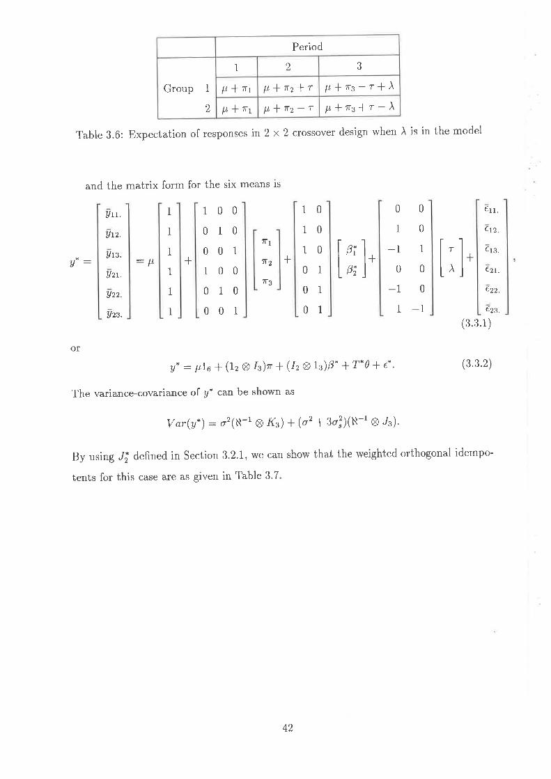
Period
Group 1
2
1 2 3
¡-r' * tt [t{'rz*r ¡t*ns-r-+À¡tltt L¿lnz-r P,*rs-l-r-À
Table 3.6: Expectation of responses in 2 x 2 crossover design when ) is in the model
and the matrix form for the six means ls
Utt.
Utz.
Ut's.
Uzt.
Uzz.
Uzs.
100 10
v: :p 1
0
0
1
0
0
1
0
0
0
1
0
0
+
I
1
1
1
1
1
10 0
0
1
I
1
1
1
0
0
0
0
0
1
0
0
i
+
0
1
-10
-11
€tt.
€tz.
€ tg.
€zt.
€zz.
€zz.
7f1
ff2
rl3[;].
pi
pi+
(3.3. i )
or
y* : þÃø -l- (12 A ft)r * (Iz Ø ls)þ" + 7"0 + e*. (3.3.2)
The variance-covariance of y* can be shown as
var(y*): a2(N-1 a 1(e) I (o' + 3øl)(N-t 8 Jr).
By using "/j defined in Section 3,2.1, we can show that the weighted orthogonal idempo-
tents for this case are as given in Table 3.7
42

i\{atrix
aö $ØJz
111 111n t
1 111 TltTùZ 111111 111
I3N
111111111
111T'l,t Tlz n 2
t 111111
a I JiØKs
2-\ -1
-12
2-l -i-12
n 21 t2 Tùl.TLZ t2
-1 1 -1 1
1
3N
2-7 -1
-12
2 -1 -1r2-11-1 2
TùtTùZ t2 nl
1 -1
a; (N-4) 8/3
1
1
I
-l-1
-i
1
1
I
1
1
1
1
I
1
-1
-1
-1
-1
-1
-1I
I
1
1
1
1
1
1
1
1
1
1
1
1
1
'lL1 'n23N
aä (N - /i) 8/rs n1n23N
2-t -1-2 1 1
r 2 -1 r-2 1
1-1 2 l-2 1
2 r I 2 -1-1r-2 1-i 2-71 1 -2 -i -1 2
Table 3.7: Weighted orthogonal matrices for four strata in the design
With this design, the total information available is
6-3 4n1n2
-32?.'(Na/-0ð)?.:{
3
43
3¡/ l:il
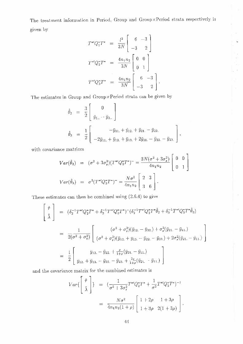
The treatment information in Period, Group and GroupxPeriod strata respectively is
given by
T*,giT"
T*,8;T*
T*'gåT*
12
3/V
6 -3-32
6-332
4n1n2
3¡ú
4n1n2
3¡r¡
0
0 il
The estimates in Group and Group x Period strata can be given by
In,
0o^,)0,:'2- Uz.
-Ut.*Un.*Yzt.-Yzz.
-2ytr. * an. * grs. l2an. - azz. - Yzz.
V ør(02) (o'+Jo!)(T.'Qir*)- : 3¡'/4nyn2
^10z: z
with covariance matrices
'")(o2 ¡3o l:ilV ar(ls) o2(7.'q;T'*)-: ffilZ:]
These estimates can then be combined using (2.6.4) to give
Q;r T.' Q;T* + ót t r*' 8år. )- (6; I T*' Q;T* 0, + 6; t T*' QäT. 0 r)lîl(o' + "?)(y'r. - azz.) * o?(yr'. - ytt.)
(ot + ")@tr. * yß. - uzz. - azz.) I2o!(grr. - vn.)
an. - azz.l #¡(Yrt. - Yn.)
an. * urc. - uzz. - uzs.l h@rt - an.)
and the covariance matrix for the combined estimates is
Ç|qr*' q;r* * jr.' eär*)-'
No2 lt+zp l*3p I4np2(r+r) ll*3p z(r+lp)
.l
1
2
i;l ÌVar{
44

In the case p -+ oo, the subject effects are regarded as providing no information and
the estimates reduce to the rvithin-subject d3. In case p 4 0, there no subject effects,
und,0r. â. u,r" combined lvith dz : ds. As p decreases, the extra information about ) from
the subjects stratum reduces the correlation betlveen the estimates of r and ). Horvever,
this correlation still remains, being 0'71 even when P : 0' If À is not in model' the
information about r in T*'Qi?* is 8n1rz zf N,, and the estimate is
(Yrr.- Us.s.- azz.I Yrs.)12,
with a variance of No2l(Snfl2). The strong covariance between î and  implies that
the variance of the within-subject estimate of r when ) is in the model is increased to
Noz f (2npz), implying an efficiency of only 25%. Even this is an improvement over the
case without baseline when there is no within-subject estimate available. Incorporation
of betlveen-subject information reduces the variance of the estimate of r to
No2(r + 2p)
4np2(t -l p)'
implying that the efficiency of the combined estimate of r when À is in the model is
No2 4np2(r ¡ p) (1 + p)
B"ru ^ NoT +2p): 44O'relative to the estimate of r when ) is not in the model. This varies from2STo (as p : 6s¡
to 50% as (p: [).
3.3.2 Two baseline measurements in the design
We shall norv examine the effect of considering two baseline measurements to lhe 2 x 2
crossover design, one before the first active treatment period and another before the
second treatment period. This case can be shown in Table 3.8 as follows.
Group
Periods
1 2 r) 4
A B
B A
Table 3.8: Two-treatment crossover design with two baseline measurements
45
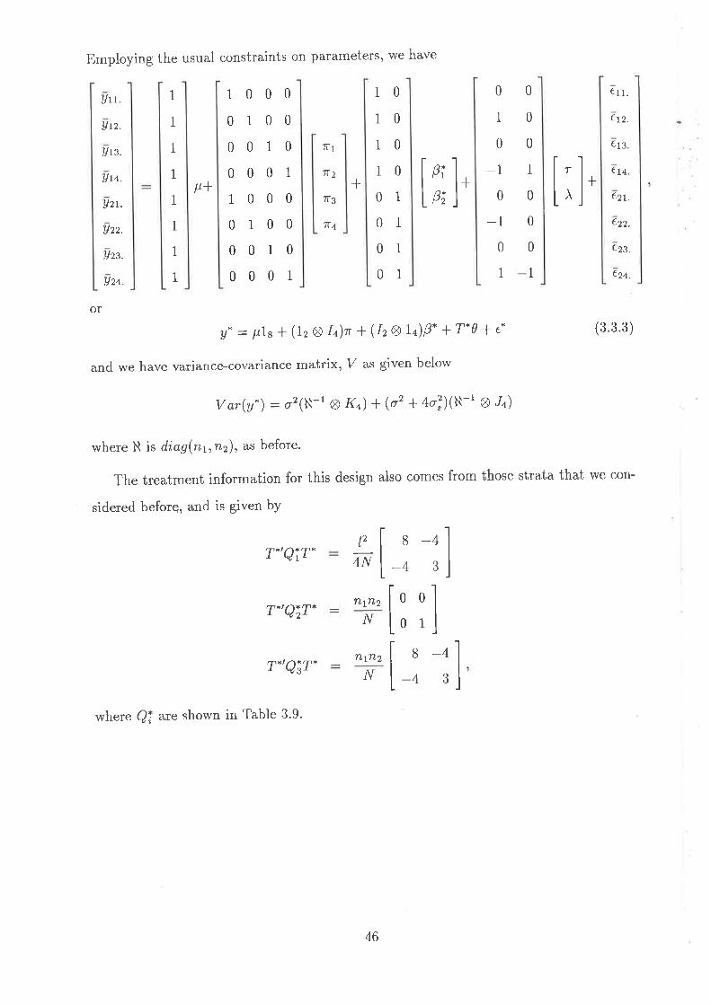
Employing the usual constraints on parametets, lve have
Urt.
Utz.
An.
Au.
Uzt.
9zz.
Azs.
Uzs,.
tt'+
I
1
I
1
1
1
1
1
01001000
00100001
10 0
1
0
-10
-10
1
€t t.
€n.
€ 1s.
€t+.
€zt.
€zz.
€zs.
€za.
0
0
0
1
1
1
1
I
1
1
0
0
0
0
0
0
0
I
0
0
0
1000
7f1
7f2
?T3
7r4
+pi
p;+
[;].010000100001 1
or
y" : L¿le * (12 A In)n + (IzØLn)p" +T*0 + e*
and we have variance-covariance matrix,, v as given below
(3.3.3)
var(y.) - o,2(N-1 g K+) + (o'* 4ø"2)(N-t I "In)
where N is diøg(nt,nz), as before.
The treatment information for this design also comes from those strata that we con-
sidered before, and is given bY
T*,QåT*
where Qi arc shown in Table 3.9.
T*,QiT*12
4N
T*,8;T* :¡ú
¡r/
n
n
8-4-43
0
0
0n
n
a1
21
i
438-4
46
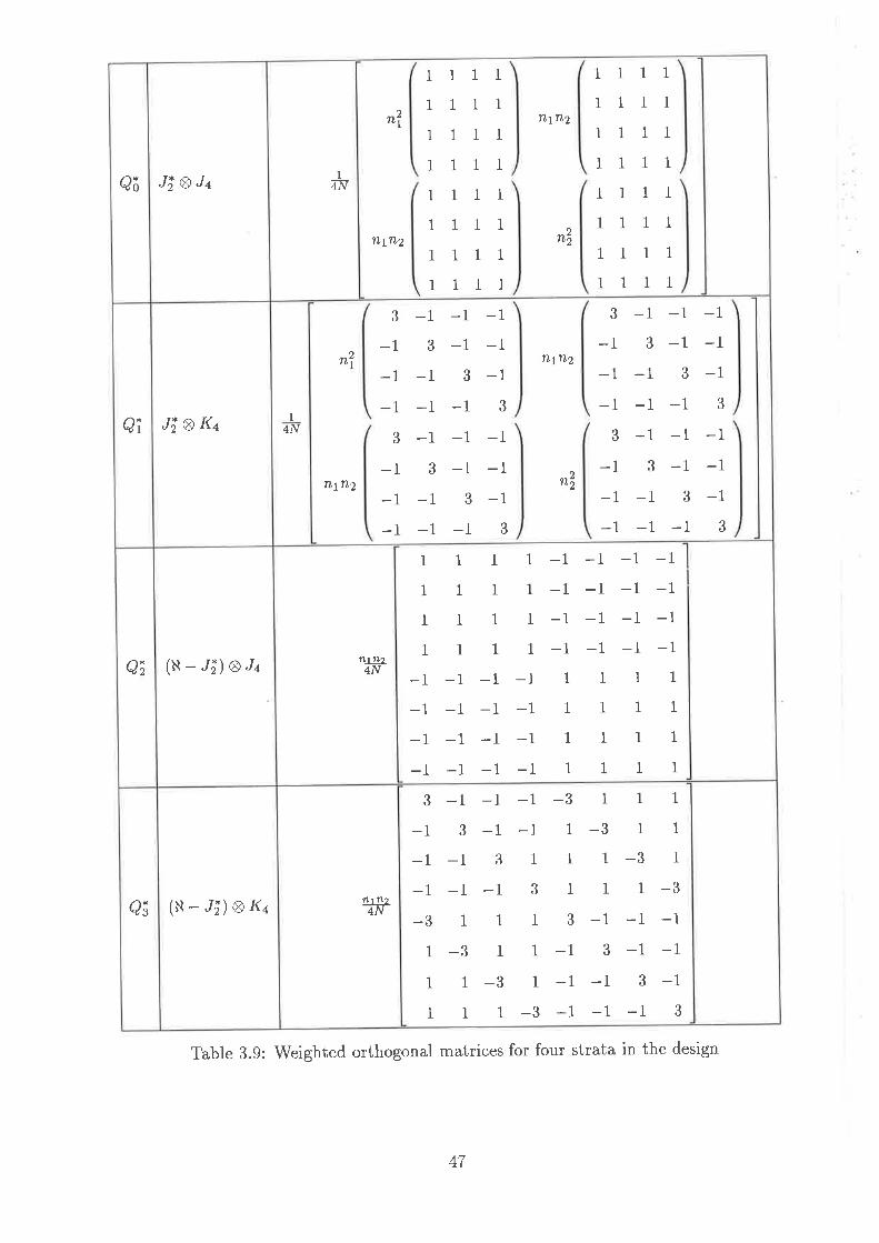
aå JiØJ+
1
1
1
1
1
1
I1
11 1
1
1
1
1
1
1
111111 1
1
1
1
1
1
1
111na
1'ltrtTL2
11 11111 111
1AF 11111
11 111ntrLZ n22
11 1111 1 1 1 1 1
n tI
3
-1
-1
-13
-1
-1
-1
-13
-1
-1
-13
-1
-1
-1
-13
-1
-1
-13
-1
-1-1
-13
-1
-1
-13
TLt-fù2
3
-1
-1
-13
-1
-1
-1
-13
-1
-1
-13
-1
-1
-1
-13
-1
-1
-13
-1
-1-1
-13
-1
-1
-13
1
4N
ntfl2 n22
a 1 JiØK4
ai (N-Jä) 8J4 n1TL24N
1
1
1
1
-1-1
-1
-1
1
1
1
1
-1-1
-1
-1
1
1
1
1
-1-1
-1
-1
1
1
1
1
-1
-1-1
-1
-1-1-1
-11
1
1
1
-1-1-1-1
1
1
1
1
-1-1-1
-11
1
1
1
-1-1
-1
-11
I1
1
aä (N-/ä) s1(4nt n24N
3
-1-1
-1
-3I
1
1
-13
-1
-11
-31
1
-1-1
3
-11
1
-31
-1
-11
3
1
1
1
-3
-31
1
1
3
-1
-1
-1
1
D-d
1
1
-13
-1
-1
1
1
-3I
-1
-13
-1
1
1
1
-3
-1
-1
-13
Table 3.9: weighted orthogonal matrices fol four strata in the design
47
The estimates in the tlvo strata, namely Group and GroupxPeriod, can be given by
Yza;I
;I
0,
0"
0
2(yt, - azz.) - (ytr.l yts. - Uzt. - yzs.)
[email protected] yu. - Utt. - yrs.) i (arr. * yzs. - 9zz. - yrn.)]
with covariance matrices
Var(02) :
Var(fu)
(o' + 4o!)(T"'QiT")- :
o2çT.'q¿T'*)-: #l
T*'Q;T* + T*'QäT* : n"::'¡/
N(oz + 4o?)
TltTùZ l:il3448
t;l
These estimates can then be combined using (2.6.4) to give
ç6;t r-' q;r* + 6lt T*' 8är.)- (6;t r-' Qir" 0, ¡ 6;r T.' QäT- êt")
Var{
f - ñ /- ''l
: ! I un. - azz.l #(grt" - an. - Uts.I vzs.) I
'l@,, lyt¿.- yzz. - az¿.) - hT,. * vrs. - vzt.- úrù )and the covariance matrix for the combined estimates is
11) : 17 unr",Q;T* * t*r-'gi?-)-t
No2 f r+sp r+4p: A;,nlT1p) l, * no ze + ap)
l;l
3.3.3 Conclusion and discussion
As we can see in the analysis of the two-treatment, two-period case, we cannot estimate r
and ) within-subject; the only combined estimates require between-subject information.
The total information in Group and GroupxPeriod strata for the two-treatment, two-
period design shown in Section 3.2 and both designs including baselines in Section 3.3
2 I
-1 I
IS
48
(3.3.4)

The only difference between the designs is the lvay in which the information about
) is lost into the Subject stratum. In the two-treatment, two-period design, 50% of
the information about À is lost into the Subject stratum, leaving a singular informa-
tion matrix. With one baseline, a third is lost into the Subject stratum,, while rvith
two baselines, only 25% is lost. Hence the baseline measurements allow us to keep
more information about ) in the Subject x Period stratum and hence improve the es-
timate of r. Thus, as move through these models, the variance of î changes from
#+t"ffifut"7effiøIf p :0, there is no change, since the total information remains the same in a1l these three
cases. Holvever, if p > 0, V ar(i) is reduced as we include more baseline measurements.
3.4 Balaamts design for two treatments
As Jones & Kenward (1939) on page 140 have pointed out, the main disadvantages of
the standard AB, BA design without baselines are that
1. the test for a carry-over effect or direct-by-period interaction lacks power because
it is based on between-subject comparisons, and
2. lhe carryover effect, the treatment xperiod interaction and the group difference are
compietely aliased with one another in the sense that only two of the three can be
estimated.
If designs with more sequences or more periods for two treatments are used, howevet,
\¡/e are able to obtain within-subject estimators of the carryover effects. The problem of
choosing the best estimates for direct treatment and carryover effects has been considered
by a number of researchers, and the designs which they have chosen provide minimum
variance unbiased estimators of the effects of interest.
One of the more efficient designs for comparing two treatments in the two period
crossover design is the design of Balaam (1968) which we consider in this section.
We will analyse the Balaam design when the subject effects are random variables with
mean zero and variance o"2 and we assume that the within subject errors are independent
random variables with mean zero and variance o2.In addition we can assumethat these
49
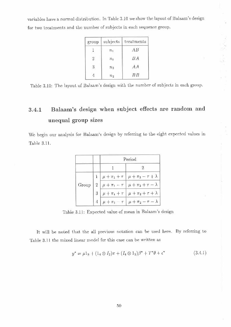
variables have a normal distribution. In Table 3.10 rve show the layout of Balaam's design
for tlvo treatments and the number of subjects in each sequence group.
group subjects treatments
1
2
3
4
Tù1
Tr1
Tr2
ft2
AB
BA
AA
BB
Table 3.10: The layout of Balaam's design with the number of subjects in each group.
3.4.L Balaam's design when subject effects a.re random and
unequal group sizes
We begin our analysis for Balaam's design by referring to the eight expectecl vaiues in
Table 3.11.
Period
1 2
Group
1
2
,)
4
p'*rt1.r ¡L,lnz-7+)þlrt-r ¡t*rz*r-)p'lr.t-l-'r p,lrz*r*)
þ*rr-r p'Irz-r-)
Table 3.11: Expected value of mean in Balaam's design
It will be noted that the all previous notation can be used here. By referring to
Table 3.11 the mixed linear model for this case can be written as
y" : ple* (1, Ø lz)t * (1¿ a lr)0. +T*0 + e* (3.4.1)
50
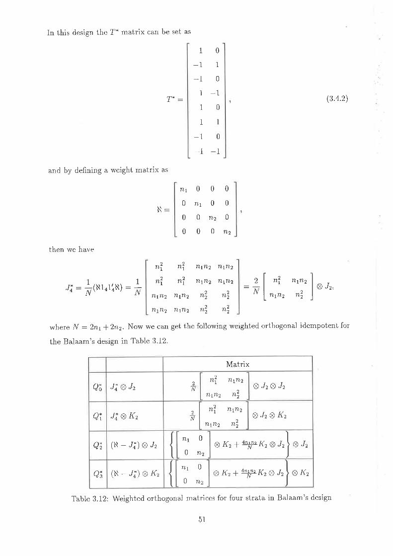
In this design the 7* matrix can be set as
t:
and by defining a weight matrix as
1
-1-1
1
1
1
-1
-1
0
1
0
-i0
I
0
-1
(3.4.2)
then we have
1
ü ¡r(N14liN)
N_
TLtTùZ
TLTTLZ
T7y 0
0nt0000
0000rù2 0
0nz
21
2I
TL
n
nl
nl
TLtTIZ
Tù tTù2
'lltTLZ
TLtTIZ
n2
TLyTIZ
TLITùZ
n"
nl
Ø Jz,1
¡\i
2
¡\i
n? fttTtz
Tlt TlZ n|nl
2
where N :2nt*Znz.Now we can get the following weighted orthogonal idempotent for
the Balaam's design in Table 3.12.
Matrix
a0 JiØJ2 tN
nl TùtTlZ
nlTùtTlZ
Ø JzØ Jz
Qi Ji Ø I{22
N
n I TLLTLz
TI¡TLZ n ) ØJ2ØI{2
a 2 (N-/;)s¿ TL1 0
0nzØ I{, ¡ ao#t<, Ø J,
) *,,
aä (N-4) Ør{zTù1 0
0nzØKz*øfl<rø1, ØKz
Table 3.12: Weighted orthogonal matrices for four strata in Balaam's design
51

The treatment information in the strata of interest can be given as
0T*,QiT"
0
T*,Q;T*2nz
ntlnz
-2n
oz(T*'QiT.r-: ç j
:i:t:t
0
0
4?IZ
T*'gäT"
2nz
4nt
-2nt nr*nz
As we can see, the rank of T*'Q|T* is two,, which is sufficient to estimate the two param-
eters of interest, so we have
0zUn. * Uzz. - Utr. - Un. * 9sr. * Uzz. - y'tt. - Yaz')
2(Ytt. * an. - uzt. - Yzz.)
V ar(îs)
Then the combined estimate for the parameters can be obtained as
T
)
T
1
4
0" : I I n"'- utz'- vzt'l vzz'- azt'* asz'* Y¿t'- a*')la L 2(v"r. - vzt. - usz' * aqt) l
and covarìance matrices of estimates are
v ar(02) : (o' + 2o?)(7.'8;T.)- : Ü#[ * "{ ]
N4ntn2 n2
48n2 n2
I : ç]*",*'Q;r* * i'.'¿är.r(;+2,?r.'8;r*02* #'.'qä7.0")
If l/ : 2(n, + nz):total number of subjects in the design, and g : ;f- as before, then
we have
{qlz(t - q)p(r + p) + (r + zp)l(an - yzt.)
- (1 - q)lzqp(r + p) - (r + zp))(úst. - yn.)
-zq(I - qX1 -f ù'@rr. - Uzz. - Uzz. + ùn )\¡zl+qçr- qxl * p)' + (1 + 2p)]
52

{q[(t - q) + (-2+ 3q)(1 + 2p)]@". - yzt.)
+ q[(1 - q) + (z - q)(t + zp)](yrr. - yzz.)
+ (1 - q)(1 + 2p)lzq(r - p) - ll(y.'. - uat)
+(1 - qX1 + 2p)l2q(r + p) + 1l(y.r. - an .)\
¡zl+qçr - qxt + p)' t (r + zfi) ,
and the covariance matrix which also depends on q and p car be obtained as
i
,.,,I i ], oz ¡ 2o2,
1l-1( T",Q;T* T*,QäT-)_
o2(LIp)(L+2p)Nfaq(l -qxr +p)2 +(1 +2p)]
Var(À)zo2fr+2qp](r+2p)
n[aq(l -qxt +p), +(1 +2p)]
\JOU\T1^) :
As we can see in Balaam's design when the subject effect is random, estimates of param-
eters of interest and variances of estimates are completely dependent on g and p. In term
of q and p there are several cases to consider.
1. When q : l, Balaam's design is just the same as the two-treatment, two-period
crossover design with n1 - Tt'2' In fact when Q : I we get the estimates of the
parameters same as given in (3.2.10) in Section 3.2.1.
2. If we let p -+ oo, then Balaam's design gives just the within-subjecf "stimates, á¡.
3. If À were not in the model, the information about r is
4n1t 4n2,
and hence the best possible variance for î couldbe o2f2N. In fact the estimate
based on within-subject differences would have a variance o2f 4n1 : 02l(2NØ), so
that this suggests we should use q close to I if we believe that no canyover exists.
4. When ) in the model, the rvithin-subject estimate of r has a variance N o2 f (8ntnr) :' o'zllQN(q(l - q)] which recovers at most 25To of the information about r, and then
ar(ì)v
o.)

only if q: Il2, \.e. ny - Tt.2. The use of between-subject information reduces this
variance too'(r-p)(r+2p)
Nfaq(l -q)(1 +p) + (1 +2p)]'
which gives significant gains in efficiency, particularly when q is near If2 and p\s
reasonably small, say less than 5. I1 p : 0 and q : I12, this achieves the minimum
varlance
3.5 Two-treatment, three-period crossover design
As Mathews (1938) pointed out, although the use of more periods causes some problems
in the experiment, there are several reasons why one may wish to extend the number of
periods in a crossover design:
1. to allow the carryover effect to be estimated (within-subject estimate),
2. to make greater use of the experiment material,
3. to make it easier to compare more treatments in the one design.
Kershner & Federer (1981) calculate the variance of estimators for direct, carryover and
total treatment effects for a number of two-treatment designs, using from two to four
periods. The various optimality results were:
o the most efficient three-period design is AB B , B AA, and
o the most efficient four-period design is AABB, BBAA, ABBA, BAAB.
Table 3.13 shows the layout of the three-period design.
Periods
Group
1 2 3
A B B
B A A
Table 3.13: Two-treatment, three-period crossover design
The model is the same as that shown in the previous sections,, but there are three active
treatment periods. Thus, by using the usual constraints on the parameters, then the
54
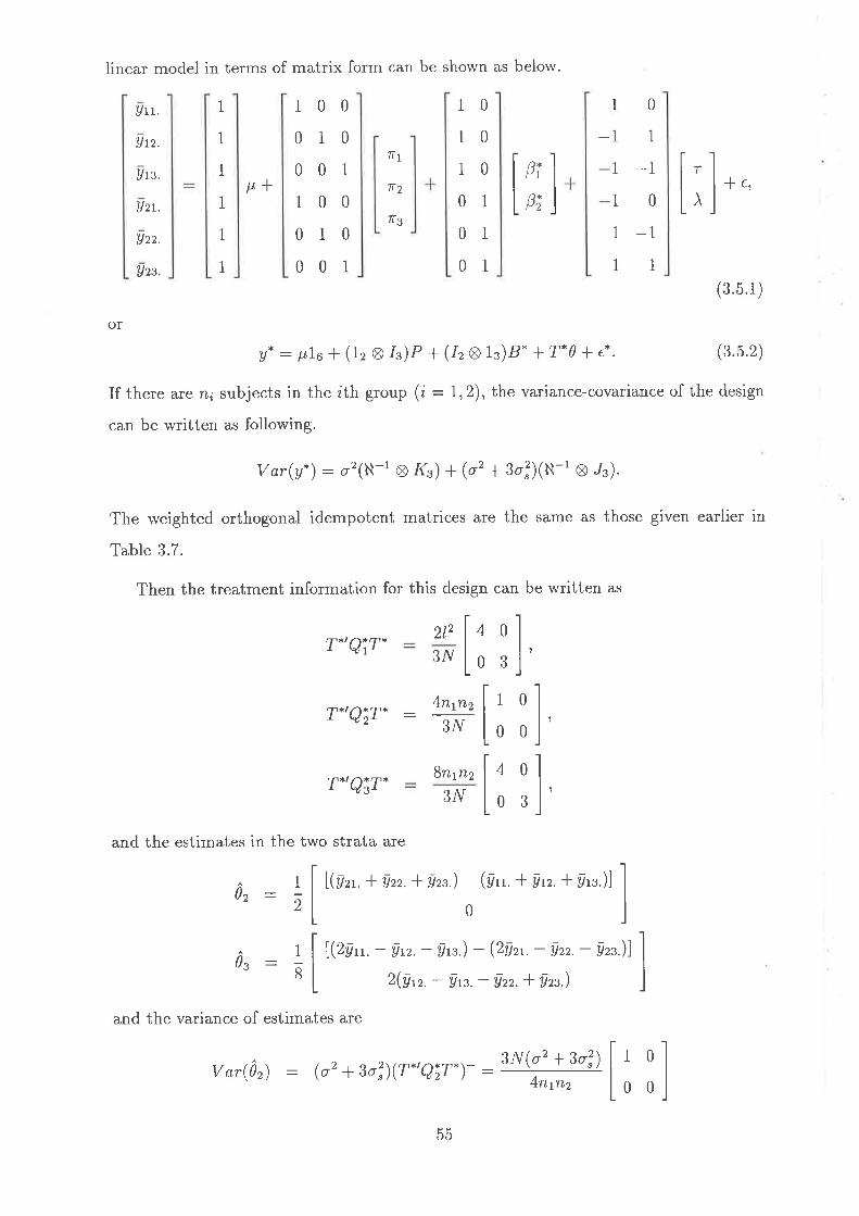
linear model in terms of matrix form can be shown as below.
Utt.
An.
Uts.
Azt.
Uzz.
Azs.
1
(3.5.1)
OI
y*: pta*(1r 8I3)P*(1241.)8. +7"0+e*. (3.5.2)
If there are ni subjects in the ith group (i : 1,2), the variance-covariance of the design
can be written as following.
Var(y.): ø'(N-1 A 1(3) -l (o'* 3o"2)(N-t 6 -Ir).
The weighted orthogonal idempotent matrices are the same as those given earlier in
Table 3.7.
Then the treatment information for this design can be written as
T*,QiT*2'.,2
3¡\i
1
1
1
1
1
1
1
0
0
1
0
0
0
1
0
0
1
0
0
0
1
0
0
1
I
I
1
0
0
0
0
0
0
1
I
I
-1
0
1
-10
-11
tt' +
7iy
7f2
7l'3
pi
p;
:l
I
1 [;]..1
1
T.,g;T* : w
4
0
'ol,0 0l
4 ol,0 3l
T*'gåT"
and the variance of estimates a e
and the estimates in the two strata are
f ,,
0, : I I l(a''"+azz'lvzt')-(an'+un'rttt')l I2l o l
0, : I I ttzl" - utz'- arc') - (2v"'- uzz'- t"')l I8 L 2@rr. - uts. - azz. * azs.) j
8nyn2
3¡ú
Var(02) : (o' + 3a3)(7.'Q;7.)- :"# l:: l
bb
V ar(0s) o'çT-'q;T-¡:#l; ;]Combining estimates from the trvo strata we have the following estimates for parameters
of interest by
t;l ( rrh"r*'Qir* * ir.'ïår"l-( rr +-Lu:7.'q;T.0r * ir-'Qä7.0")
Then the estimates of two parameters can be obtained as
1
2(3 + 8p) l(r + 4p)(gn. - an.) + (1 + 2p)(-vrr. - arc. * azz.* vzs.)l
^1¡ :,lytr. - Uts. - Uzz. I Yzs.),4
and the covariance matrix for estimates is
v.,(l I l,: !!f r# 'l'-''LÂl' Bn1n2 l o rlAs we can see the estimate of direct treatment is obtained from all data but it depends on
variances and the variance of estimate not only is less than the corresponding variances
in the standard design, that is, AB vs B Abú also the correlation between them is zero,
that is, î and i ir itrd"p"ndent. In addition as we can see in this design the information
in Subjects stratum is now about r rather than À. With this design the proportion of
information on r and À lost into the Periods stratum is
2/2 2(q-n2)2 rt o \2
5"t", +2P :
4r, ¡ -, - \L - zq)
The proportion of treatment information lost into the Subjects stratum is $ : |, so
there is not much treatment information to recover. This can be demonstrated by an
equivalent formula which shows how little the estimate of r is changed:
î : â",',.- r+"- {(zvrr. * vn.* vrs.) - (2arr. * vzz.+ vzs.)}. (3'5'3)ð(r -t- öp)
and the variance of â is smaller than that of the within-subject estimate by a factor
s(1+sp)/{s(s*8p)},
which varies from 8/9, when p is small and we recover all the between-subject variation,
to 1, when p is large and there is no useful information to be recovered from between
subjects.
T
bb

Chapter 4
A Bayesian analysis for the general
crossover design
4.L Introduction
By sharing information among components of a statistical assessment and possibly in-
cluding external objective evidence and personal opinion, Bayesian methocls have the
potential to produce more efficient and informative statistical analyses than those based
on traditional approaches. In the Bayesian approach, the likelihood function is multiplied
by another function due to prior belief in the values of parameters under consideration.
This product gives us a new function which we refer to as the posterior distribution.
Then in a Bayesian analysis lve should consider the following concepts
1. an observed random variable or vector y,
2. a parameter vector 0,
3. the conditional density f @lg) of y given 0, and
4. the marginal density p(d) which is called the prior distribution of d.
In the two treatment, two-period crossover design, there are a series of papers whìch
have used the Bayesian approach. Racine et al. (1986) and Grieve (1985), for example,,
presented a Bayesian analysis of the two-treatment, two-period design and Grjeve (1986)
used Bayesian analysis for this design when there are two baseline measurements in the
5(
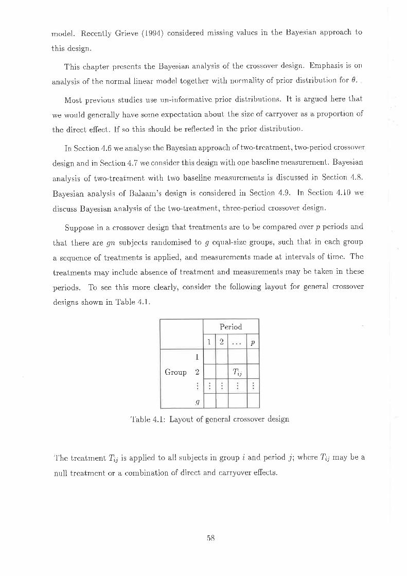
model. Recently Grieve (1994) considered missing values in the Bayesian approach to
this design.
This chapter presents the Bayesian analysis of the crossover design. Emphasis is on
analysis of the normal linear model together with normality of prior distribution for 0.
Most previous studies use un-informative prior distributions. It is argued here that
lve would generally have some expectation about the size of carryover as a proportion of
the direct effect. If so this should be reflected in the prior distribution.
In Section 4.6 we analyse the Bayesian approach of tlvo-treatment, two-period crossover
design and in Section 4.7 we consider this design with one baseline measurement. Bayesian
analysis of two-treatment with two baseline measurements is discussed in Section 4.8.
Bayesian analysis of Balaam's design is considered in Section 4.9. In Section 4.10 we
discuss Bayesian analysis of the two-treatment, three-period crossover design.
Suppose in a crossover design that treatments are to be compared over p periods and
that there are gn subjects randomised to g equal-size groups, such that in each group
a sequence of treatments is applied, and measurements made at intervals of time. The
treatments may include absence of treatment and measurements may be taken in these
periods. To see this more clearly, consider the following layout for general crossover
designs shown in Table 4.1.
Period
1 2 p
Group
I
2
g
T¿j
Table 4.1: Layout of general crossover design
The treatment T¿¡ is applied to all subjects in group i and period j; where ?,¡ may be a
null treatment or a combination of direct and carryover effects.
58
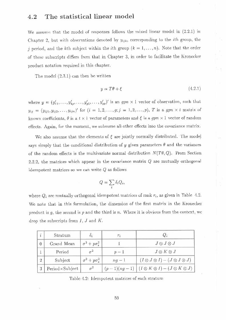
4.2 The statistical linear model
We assume that the model of responses follows the mixed linear model in (2.2.1) in
Chapter 2, but lvith observations denoted by y¿jt , corresponding to the ¿th group, the
j period, and the kth subject within the ith group (k : 1, . .. ,n). Note that the order
of these subscripts differs from that in Chapter 3, in order to faciliiate the l(ronecker
product notation required in this chapter.
The model (2.3.1) can then be written
y:70'f€ (4.2.\)
where a : (U1t,...,a1p,...,U'¡r...rU'no)' is an gpn x 1 vector of observation, such that
Aij : (A¿jr,ynjr,...)A¿jn)t for (i : I,2.,-..,9)i :1,2,...,p), T is a gpn x ú matrix of
known coefficients, 0 is a f x 1 vector of parameters and { is a gpn x 1 vector of random
effects. Again, for the moment, we subsume all other effects into the covariance matrix.
We also assume that the elements of ( are jointly normally distributed. 'lhe model
says simply tirat the conditional distribution of y given parameters d and the variances
of the random effects is the multivariate normal distribution N(70,Q). From Section
2.2.2, the matrices which appear in the covariance matrix Q are mutually orthogonal
idempotent matrices so we can write Q as follows
Q:Ð6nQ'
where Q; arc mutually orthogonal idempotent matrices of rank ri, as given in Table 4.2.
We note that in this formulation, the dimension of the first matrix in the Kronecker
product is g, the second is p and the third is n. \{here it is obvious from the context, we
drop the subscripts from 1, J and K.
? Stratum 6¿ T¿ Q¿
0 Grand Mean o, + po,, 1 JØJØJ1 Period o t p-l JØKØJ2 Subject o' + po? ng -r (IØJs1)-(JØJØJ)3 Period x Subject o2 (p-1)(ns-1) (181(S1) -(/s1(S/)
Table 4.2: Idempotent matrices of each stratum
59
As before, an analysis of this model to determine the estimates of d in the various
strata, lvould not include i : 0 since there is no useful information about treatment
parameters in the Grand l\,{ean stratum. Throughout this chapter, therefore, lve will omit
the term for ôs. We may, however, include i : I if there lvere information available, in
the form of ol, which would allolv recovery of the treatment information in the Periods
stratum. Generally, however, we would set o2n : ñ, so that ár : 0 and the Periods
stratum would not contribute to the estimation of d.
The fact that all n observations in a group have the same treatment regime implies
that
E(y):ry81:T*0Ø1 (4.2.2)
and
Var(y): q,
where q i. {ry¿¡} in standard order and 7 : T* I 1,r. In order to work on means let us
define the average of responses by
1
n(1s181)'y (4.2.3)
4.3 Likelihood and parameter estimation
The likelihood function becomes
1L p@10,Q): l}aÈerp{ fu-rÐ'Q-'fu-re)j
2(4.3.1)
fr.uo î"
"*, - ;å*å,, - ro)' e¿@ - rÐj
slnce
tat det(Q) :3
II ¿I.i=O
IQ-r t Q¿
i=1 6¿
To simplify the exponent term in the likelihood function we define
a:Gy+(I-G)y;
60
Maximising L can be achieved by maximising the logarithm of .[ which shall be
denoted by, /, namely
Sz Ss(4.3.4)
and the maximum likelihood estimate of 0 is obtained by differentiating I and equating
it to zeroat
(4.3.5)i=l
f rolog 6,-t Ðti=l lrn - r-i)'Qî@ - r"o)j - Z(o2 * no2") 2o2'
a0 Ð lr.'orrn - r.o) -- o.
\ : yr.. - uz..- t (^, t!+r),rvhere m: Nl(U n2), and an estimate of the variance is provided by
sz - o2(l +Zp)xlrr^_r¡.
,1I: -,
If we define Q* :ÐiQi, then the solution is obtained as
0 : (7"'Q*T*)-tT*'Q*y, (4.3.6)
and the distribution of d given d is
Ole - N {0, (T"' Q*?*)-t},
provided o2 and o2 + po! are known. Using the marginal likelihood for ^92 and 53, we
obtain
ur+pã?: I S, ,1.
'g(, - \)t'
;z: ' St
tLs@-t)(n-1)"
providing unbiased estimates of ø2 and o2 + po2, respectively. S, has g(n - 1) and ^93 has
g(p - 1X" - 1) degrees of freedom. If in fact the rank of T* is less than gp, there will
be sorne degrees of freedom available which may provide further estimates of o2 andf or
o' +po?. In general, they will have relatively few degrees of freedom and hence we choose,
for simplicity, to ignore this information.
If o2 and o' + po? are unknown and have to be replaced by estimates, clearly the
multivariate Normal distribution now becomes similar to a multivariate ú-distribution. In
literature, in this regard, little has been done in general. However, in the two-treatment
two-period case the combined estimate of ) has the distribution
62
Hence()-À)
- tz@-t\.mSzla{@ - 1)}
Holvevet,^ l, / m.ø2lt*p)\.î : ,furt. - an.) - t trt' -o )
and rve do not have aX2-distribution to estimate o2(\*p).The estimateof this relies on a
combination of 52 and S¡. The result of this, as Grieve (1985) shows in Bayesian context,
is that the joint distribution of (î, i¡ ir u combination of two independent multivariate
f-distributions, which provides a Behrens-Fisher distribution. Patil (1965) shows that
this is well approximated by a multivariate f-distribution.
4.4 Bayesian analysis
Suppose that the prior of 0 is 0 - l{(do, X6), where X6 ma} be singular. Now we discuss
the Bayesian approach for our model in two sections,, one when Ðs is a nonsingular
covariance matrix and another section when it is a singular matrix.
4.4.t !s is a nonsingular matrix
In this case of a design with g groups and p periods, when X6 is full rank,, by following
Lindley & Smith (1972) and using Bayes theorem, the posterior distribution for d is given
by
010 - N(ïe,Ðò (4'4.r)
where
1Var(010):E, (t T"'Qir* + r;t)-t
6¿
and
E(010):0e : tÐf,r.'qîr- +tt')-' ,\lr.'Oîa +>;'r,o¡. (4.4.2)
The posterior mean is a vector-weighted average of the prior mean d¡ and the maximum
likelihood estimate, á. The weights are respectively the prior information matrix X;1
and the inverse of the covariance matrix of the maximum likelihood d. The posterior
63
covariance matrix is the inverse of the sum of these weights, and the posterior cova lance
matrix is smaller than either the prior covariance E¡ or
1
6¿(t T-'gîT-)-t
in the sense that
(Ðlr-'qir.)-'- (: lr.'orr. + xl')-',
is non-negative definite. It follows that
Var(d'010) 3 Var(d'l), (4.4.3)
for all vectors d.
In general,l suppose we are interested in some contrast d'0. For example, if d :
llr,rr,Tz;Àt¡À2]'and rrye are interested in the posterior distribution for (1 - 12), then
Var(r1_ "2ll) : {(T*'Q*?. * Xõt)-td,
where d: 01-1 00 . Then the posterior distribution of (rt - rr) would be
(r1 - r)lâ - N (d' 0p, d'Epd) (4.4.4)
4.4.2 Es is a singular covariance matrix
If the covariance matrix Ðo is not full rank, this implies that certain directions in the
/-dimensional parameter space have no prior information. This can be expressed by
regarding the information matrix Xo as having zero eigenvalues in these directions. Thus
we write k
Xo: DJ.im¿mtn- MIM',, (4.4.5)
where k : rank(Eo),m'¿m¡:6¿j,-n";- 6¿¡ is the Kronecker delta. Then the irrformation
matrix or g-inverse with minimum rank is
kti=l
(t
iTTItàn'¿\--uO
and the posterior distribution for d is Normal with
T,,|
1Var(010) : t',
64
6¿T"'QiT* + Ð0)-t
and
E@p¡ : e, (D T"'?ir* + Et)-'(Ð T-'Qiv + Ð;oo). (4.4'6)
On all occasions we will use the minimum rank symmetric A-inverse of Xs.
If o2 and o' + po? are unknown and have to be replaced by estimates, then O¡O it u
mixture of two non-central multivariate ú-distributions. There is little on this in the liter-
ature. However, Grieve (1985) considers the two-treatment, two-period crossover design
with l/ subjects and, possibly, unequal group sizes of n1 and D,2, and from the classical
analysis approach of this design, he summarises the following independent distributions
for all parameters in the model.
1--ð;
1
ò¿
\lt, ^) ry
\Trr ) ry
SzN
SsN
¡/i(p, )), ÐrÌ;
N{(r, r - À12),Es};
(o' + 2o?)x?u-r;
o'x'¡v-,
N-12
where
Ez : (o, + ,"?ll * l' 'ln f ,
I tl+ *12 )
xs : o'l *l'
'/t I ,
I tls *14 )
where N : nt * nz, m: Nl(u n2) and l: (u - n2)f (npr). By appiying the following
un-informative prior for al1 parameters in the model
p(lt, ¡r, r, À, ..2, o3) o ñ+tð,Grieve (1985) shows approximately that the marginai distribution of Ór: , - \12 and
ó2 : ^12
can be obtained as
p(ót) o(
8(ó, - ^12)'
Jv-1--Tp(óz) o( Sz1
n'r
By referring to the result of Patil (1965) who showed that, if /1 and þ2 arc two param-
eters lvhich have independent shifted and scaled ú distributions, then the sum of two
65
parameters has Behrens-Fisher distribution, Grieve (1985) then shorvs that r : ót I Óz
is approximated byt+l
2
p(r) x
rvhere
(Ss*s2)'?(N-6)r 4
s3+s3(/-z)(s, 1s,)
Law (1987) in his thesis develops a Bayesian analysis of higher-order crossover designs.
For a subset of the parameters, d, of length r, he use a prior distribution lvhich is
multivariate Normal distribution, with mean 0s and covariance matrix o2Ðo. He also
uses a Gamma Distribution for the prior of ø2' Thus
hN -4
p@2) o(
p(01"\ o(
0e
x
t:l
r:lwhere d, 0,00 and Xs are assumed known. Then the prior density of 0 can be derived as
r i .2aÐ^r l-tt+")p(0) x
lr + firo - vù''qr; (d - d.)l u
-," lro,
\r",r,f , Ø.4.7)
a multivariatel-distribution, where r is dimension of 0. He then uses the within-subject
estimate of d as 0lg - N {0,o2(T'T)-t} and shows that the marginal posterior density
for 0 is also the multivariate ú-distribution
ïly - t,l|r,Ep,u I r ! 2al,
where
p
: (T'T + xt')-'(?'rA + z;r0o)
: a(T'T + xtt)-t,
and
lzp + ¿'ol,t0o + a,y - (T,Têt+ t;1p0),(T,T + Ðtt)-t (T'T0 + xo'do)] ,*- (r*r*2QLand u is the degrees of freedom of .9s. The only reason this method works is that Law
(1937) makes the somewhat unusual assumption that the prior for 0 involves the unknown
ø2. Without this, the multivariate f-distribution is not obtained. Similarly, in our case,
to include the betrveen-subject estimates as well, the complication is that there is a factor
o2(t + pp) and,, unless p is known, the terms do not combine conveniently.
66
4.5 Choice of prior distribution
We have four strata in the crossover design which may contain treatment information,
wìth weights ð¿(i - 0,...,3). As before we a e generally not interested in using i : 0,1,
although we might use i : 1 if we had a prior distribution for the period effects n.
In addition in practice the 6z : o2 + po? and á3 : 02 ate not known and we should
replace these terms by their estimates or use prior distributions and integrate them out
if necessary.
In the following sections we will show the Bayesian analysis in certain crossover de-
signs. But first, we need to consider the type of prior distributions which might be used
for (r, )).
As we showed in the previous chapter, the expected values of responses in the two-
treatment, two-period crossover design when the period effect is random can be repre-
sented in Table 4.4.
LL+r p,-r*Àp,-r p*r-À
Table 4.4: Expected vaiues of responses in two-treatment, two-period design.
In our models, the difference between the two treatments A and B is equal to 2r, and
the difference in their carryover effects is equal to 2À. Suppose that treatment B is a
standard on-going treatment, like a baseline, for which the true value is ¡lo and for which
no carryover effect is expected. If we now look at the way treatment A departs from this
baseline, we can model the four means by the revised Table 4.5.
þo*2r ¡ts!2À*rl-to L¿o l2r I r
Table 4.5: Expected values of responses when treatment B is a standard treatment
This table provides a model in which the active drug A has a treatment effect relative
to baseline and in which we might expect any ca ryover effect to be a percentage of that
treatment effect. Such a relationship of treatment and carryover effect can be shown in
67

Figure 4.1, where our prior distribution for the carryover effect is that it is a proportion
k of the treatment effect, as expressed by
P()lt) - N(k''ozò' (4'5'1)
where k is a smal1 value, probably in the range (0 - 0.5) and øfr expresses our degree of
prior certainty about that relationship. We note that the case k : 0 corresponds to the
situation considered by Sehvyn et al. (1981). If we assume an un-informative prior on r,
the joint distribution of À and r is
p(r, À) : p(r)p()l r) x erp{-t^ - kr)'zlzol) . Ø.5.2)
Figure 4.1: Conditional distribution of carryover effect given direct effect
À
ÀÃ.2t
"c
Now we can write
-k T(À - kr)21 (4.5.3)
1 À
so that the prior density can be represented by a singular bivariate Normal with infor-
mation matrix
\]-uoIc2 -k-k1
202o
I,02o [' ^rli; ti
Following (4.4.5), this can be represented as a singular covariance matrix
,,:r5l!'rïl68
4.6 Two-treatment, two-period design
In Chapter 3, we obtained betrveen-subject and within-subject estimates for d in the
Group and the PeriodxGroup strata as
/V
2
0,
0,
l:, 1 #l_: il)110
0
Ut.. - Uz.
1(dr. - dr.) (2r - À)
We noted that, in combining these estimates, we needed to weight d2 uttd d, by th"
inverse of those covariance matrices, using a minimum rank g-inverse in cases where the
covariance matrix is singular.
When this is extended to include a prior distribution for d, the same principle applies,
so that ifd - l/(do, Eo), (4.6.1)
where Xs ma1, be singular, the posterior distribution for d, given (o',,p), is given by
(010,o2, P) - N(00,E), (4'6'2)
where
\-l-4OEr: (T*tQ*T* + -1)
and
0e : Ee(T"'8"7.d+E;do)
: Eo{(T.'Q*?. + Ð;)d + t;(8. - rî)}
: l- to>;Q-eù, (4.6.3)
so the mean of the posterior is shifted from á towards ds depending on the distance
between d utrd 0s and the strength of the prior information.
4.6.I Posterior estimates
Combining the two estimates appropriately with the prior for (r, À) we obtain
r, lr,,,,l n -zl 2n1n2 f o ol ,-rlk'-*ll-'Ep: t"t'L-, ,]*ñ@¡ralo,l*al-r ,ll69
k2 -k l.[:i]]
k
-1
l.,l4-2
-k1 -2 1
1
where b: (1 +2p), and ¿ : No2(1 l2p)lQn1n2o2). Then, after simplification,
Ð (4.6.4)
where
A': alb(2 - k)' + l*2) + +u.
If we assume that do:0, the posterior distribution for 0 \s N(îr.,Xo) where Xo is given
above and (4.6.3) implies that
p: {.[; å].,[;;].1;:]]
Ir-:llt
; I . å
I ; ] t-t +b(z-k)(zi-irr
0
lri-*ork)
k)2b
1.,[; ')+ 1 0p
0 -1
2
If  : kî then the estimate is unchanged, as would be expected since the data is consistent
with the prior distribution.
In other cases, however, the maximum likelihood estimate á is shifted towarcls the
line ) : lcr.
lL, - ak{k - b(2- k)}lâ r a{k - b(2- k)}i2abk(2 - k)î+ {A - 2ab(2- k)}i
(4.6.5)
(4.6.6)
Now, k will typically be smal1, certainly less than about 0.5, and ó is at least one. Thus,
the last term is dominated by the fact that most of our information in the data is about
(2ì - i) u"d there is relatively little information about ).
The two particular cases of interest here are (i) when a : 0 in which case there is
no prior information and the estimate reverts to d, and (ii) when c -+ oo, for then we
know that ) : kr and the estimate has to lie along that line. The above formula then
70

simplifies to
0p1
l.l:îl)'
(4.6.7)k
so that the posterior estimate for ) is k times the posterior estimate for r. As ao2 varies
between these two extremes, the posterior estimate (4.6.5) moves along a straight line
joining d and the point (4.6.7) on the line ) : kr.
4.7 Two-treatment, two-period with one baseline mea-
surement
This section presents the Bayesian analysis of the 2 x 2 crossover design with one baseline
measurement taken before a treatment is given to the subject. We consider that the
experiment yields complete data on n1 subjects in the first group and n2 subjects in the
second group.
Frcl-i Chapter 3 for this design we obtained the following between-subject and within-
subject estimates from Group and GroupxPeriod strata respectively
0,
03
1,,
,1,
'{l
0
Uz )
An. - An.l Yzt. - Azz.
n. * ytz. - 2yrr. - Uzz. - Azs. I ZAzt
0
t)No2T
)
2336' 4n1n2
If we apply the joint prior density in(4.5.2), then these estimates can be combinedwith
the prior for (r, À) to obtain
\-f"pl 4n1n2
3No2
6-3 1
r-]) '
l:'ro2o+
-32
lcz -k].,1
6-3-k1 -32
77
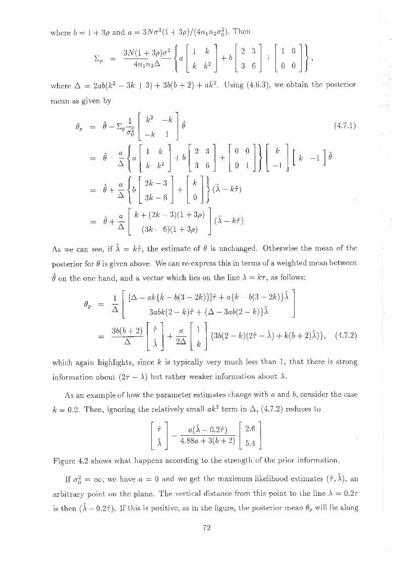
where b: I * 3p and a : 3No2(l + 3fl1(anp2o2o). Then
10rup00
rvhere tr : 2ab(k2 - 3k + 3) + 3b(ó + 2) I ak2 . Using (4.6.3), rve obtain the posterior
mean as given by
r##{.[; ;].,[: :].I
0 k
0
l)
0-E,hl:'- ,-1,
â-x{.1;;1.,i::].1
0e
{, l;-:l.l:l}l**ek-s¡1r+spt IL (s¿-6X1 +3p) j
¡CLo+^
a+Ã
(4.7.r)
illi k 1 0
-1
i( ki )
:0 (À - kâ)
As we can see, if  : frâ, the estimate of d is unchanged. Otherwise the mean of the
posterior for d is given above. We can re-express this in terms of a weighted mean between
d on the one hand, and a vector which iies on the line À-_ kr, as follows:
0o : + I to - ak{k- ó(3 - zk)}lî + o{k- ó(3 -^ zr'l1i l' a L ¡o bk(z - /c)î + {a - 3øó(2 - k)}) j
:3b(ó+zllrl n ftltf Lr ]-tà L* lttut'
-k)(2î -)) + k(b+2)))], (4'7'2)
which again highlights, since k is typically very much less than 1, that there is strong
information about (2, - )) but rather weaker information about À.
As an example of how the parameter estimates change with ø and ó, consider the case
k : 0.2. Then, ignoring the relatively small alcz termin A, (4'7.2) reduces to
t^t ^ l-^^llîl o(À-0.2î) 12.6 I
4ssc+B(b+2) | ILil rsalFigure 4.2 shows what happens according to the strength of the prior information.
I1 of, : oo, rve have ¿ : 0 and we get the maximum likelihood estimates (î, i), an
arbitrary point on the plane. The vertical distance from this point to the line ) : 0.2r
is then 1i - O.Z;;. If this is positive, as in the figure, the posterior mean 0o will lie along
72
Figule 4.2: Relation between posterior estimates lvhen k :0.2
À
?'=0.2r
(r,À)
T
2(yt . - azz.) - (ytr. * an. - uzt. - Yzs.)
Z(Etr. I ytt. - at. - aß.) * @rr.l yzs. - Uzz. - az+
'c( À)
À-0.2r
'c
the steep angled line, and will be somewhere between d and the point denoted by (i, i)in Figure 4.2. This point is the one obtained as ø -+ oo.
4.8 Two-treatment, two-period lvith two baseline mea-
surements
This section presents the Bayesian analysis of the 2 x 2 crossover design with two baseline
measurements which have been taken before each treatment is given to the subject. We
consider that the experiment yields complete data on n1 subjects in the first group and
n2 subjects in the second group.
From Chapter 3 for this design we obtained the following estimates
0z
T
)
3448
No2
'8n1n2 l)If we apply the joint prior density in (4.5.2), then the combination of these densities using
Bayes theorem can be given by combining the two estimates appropriately with a prior
I ,')
for (r, À) to obtain
\-up
0e -{x
8-4 1 ll ïl)'ol+-43
-1N(l + 4p)o' k2 -k l.l:il)TltllZ -k1 -43{,1 ]-,1
8-4
where b : 1 * 4p ar'd a: No2(l * afil@p2øfr). Then
Ðe: ryy{, l;;1.,1; :].1; :l}rvhere [: ab(3k' - 8lr + A) + 8ó(ó + t) * ak2. The posterior distribution is N(do, Xr),
lvhere
0_1 I k2 -kp 0
ofi -ki
k
k+
À
)
u-x{"
,.å{,
,.ål_
4
8 l.l; :lllll rk-1 ê
)T
+ (3k - 4X1 + ap)
(4k-8)(r+ap))
We note that if \ : kî, the estimate of 0 is unchanged. However, in general, for different
values of a, the posterior mean for d will lie along a line between g and a point on the
line ) : kr:
^ I I t¡- ak{k-b(4-3k)}lâ +o{k- b( -r¿lli IaP : ; I A^ALrr) L\êrJ,A, I. Al A"bk(z-k)i+{A-4ab(2-k)}) I
: qilr I ; I
- å I ; l "o"
- k)(zî- i) + k(b +1)i)i' (4.8.1)
4.9 Bayesian analysis of Balaam's design
We have seen in Chapter 3 that Balaam's design is an optimum design to compare two
treatments. In this section rve consider the Bayesian analysis of Balaam's design when
we will restrict ourselves to n subjects in each sequence group.
74
From Chapter 3 for this design rve obtained the estimates as
1i: AL
ru ,,{
0z
Azt. * Uzz. - Utt. - Atz. * 9sr. * Usz. - y¿t. - y¿2.)
2(Ytt. * atz. - Uzr. - Yzz.)
i'l o'+zo?l t -1 lìL^l'',;L_,,11'Utt. - Utz. - Un.I Uzz. - Av. * Usz. * yat. - y+2.)
2(Y"r. - Uzt. - U+2. * Yq.)
I'l "'lt'llL^l'z"lt r)l
If we apply the joint prior density in (4.5.2), then the combinations of these densities
using Bayes theorem can be given by combining the two estimates appropriately with
the prior for (r, À) to obtain
1
2n
"'
2-l +l; l)'i].
ll)',']2
1
4
+
le2 -kFap
-1 -k1
k2 -k].,1
2
-k1 1 1
Ðe:4#{. ll-;i ]-,ll ;l-where L,: abl& - t)'+ 1l + ø[(k + 1)2 + r]+ (2b2 + 6b11;.
The mode of the posterior distribution when go : 0 is
where b: I ! 2p and a : o2(l | 2p)lQnoo). Then
0p : 0-Ðo 0
(1 + k) + (k - r)(1 +2p)
-(2+ k) +(k -2)(1 +2p)
1
-1
tO,0-l
â**
rO,o+^
;l,ll
Â
1 -1 k-t ]
,î
]r-1
+2 -1
kì' )
(5
1i-m;

Norv if À : kî, the estimate of d is unchanged. But again we can shorv that, as ø changes,
the posterior mean moves along a straight line joining (â, i) and a point (ã, i) on the
line À : kr.
[A - øk{l + k - ó(1 - k)}]î + ø{1 + k - b(1 - k)}
ak{2 -r k - b(2- k)}f + [a - a{2 * k + b(2- k)i]0e: * ìl
l;1.*l1
kl{2 + k + b(2 - k)}î + o{1 + k -ó(1 - k)iÀ)1,
4.tO Three-period designs with two groups
From Chapter 3 for this design we obtained the estimates as
ê" : ilUn,' * vzz' r v,*')
; ,n" t vn'+ t" )f
]
'{[;] "s#dl;:l]â, :
å | "n' ' -
î','n,,-:,] --?,n,'*
n,t: *''
]
'{l .i^,,] **l; ;]}If we apply the joint prior density in (4.5.2), then the combination of these densities using
Bayes theorem can be given by combining the two estimates appropriately with the prior
for (r, )) to obtain
1 -kl)'
l)
il)
0 1
-1t{ -k].,1;:] +
1000-k1
where b:2(l+3p) and a: No2(I*3fi1@n1rro'ò. Then
\-P
0
(l)
0
where L^ : ab(3le' + 4) + I2b2 i 3b * a. The posterior distribution is then N(|p,Eò,
where
î, _ zo0p
tCL0-T
â*lt
ls o
L' 4
I.'-
+00 k
01 1 '].âk
3/ú(1 + 3p)
-4(1 +3p) -1
Now if \ : lcî,, the estimate of 0 is unchanged. But again we can show that, as o
changes, the posterior mean moves along a straight line joining (î, i) and a point (i, i)
on the line À : lcr.
kî.
1
^0e
(L,-labk')î+Sabk\ak( b+ 1)â + {A - a(4b+ 1)}i
3ó(4b + 1)(4.10.1)
A
In general, in all these examples, the case 03 : 0 will produce an estimate satisfying
À: kr by moving along a straight line from (â, i) to the line ) : ler. lf ol10, then the
posterior mean is only part of the way along that straight line, as shown in Figure 4.2.
I ; ] . å [ ; ]
*',"r1)kr+3ablci)r,
(t

Chapter 5
Analysis of a two-period crossover
design for the comparison of two
active treatments and placebo
5.1 Introduction
This chapter considers the analysis to the design in Koch et a1. (1989) involving three
treatments in two periods. Those authors were considering a situation involving a chronic
health disorder, in which two treatments were active agents (labelled A and B), with the
third treatment being a placebo, labelled P. In their paper, the authors supposed that
there weÍern subjects in each of the groups 1 and 2, which receivedthe activetreatments
in the order AB and BA respectively, for every one subject in each of the groups 3,4,5,
and 6 which received the treatments in the order AP, PA, BP and PB respectively. In
this chapter, we will suppose that m: l.
The analysis given by Koch et a1. (19S9) considers several models which have either
no carryover effects, equal carryover effects for the two active treatments, or distinct
caryover effects for the two treatments. We note particularly that they only consider
between-subject estimates and, as we show ìn this chapter, there is considerable advantage
to be gained by recovering the betlveen-subject information.
This design is considered further by Laird et al. (1992) who consider two-period
crossover designs in general and who argue for the combination of the two components of
78

the variation. While they consider the variances of the estimates in the different strata,
they do not look closely at the covariance matrices of the estimates in the different
strata, nor do they present either the combined estimates or the covariance matrix of the
combined estimates.
5.2 The linear model
Following the method in Chapter 2, \rye assume that Y;¡¿ is a random variable with the
observed value g¿¡r which follows the mixed linear model given there. The layout is shown
in Table 5.1. We shall suppose that the groups each have n subjects, thus there N : 6n
subjects.
Table 5.1: Layout of design with two active treatments and placebo
Following the model in Section 2.3 of Koch et al. (1989), we shall use a model in
which
¡ there is no residual effect for the placebo,
r the direct effects of the placebo, A and B are respectively,0, Tr and 12,
o the residual effect ofplacebo, A and B are respectively,0, )r and )z
We shall see shortly that the information in the design separates conveniently into a
component corresponding to the average treatment effect lor A and B and another cor-
responding to the difference between the effects of A and B. Accordingly, we define:
Group Period
i 2
1
2
J
4
5
f)
A B
B A
A P
P A
B P
P B
79
o rs : (rt + 12)12 and À6 : ()1 + ^2)12
as the average effects of treatment and
canyover respectively, and
o rp : (r1-r2)12 and )¡ : ()r -Àr)12 as the half difference betrveen direct treatment
and carryover effects of the two treatments respectively.
From the twelve cells which are the combination of six groups and two periods, the
expected values corresponding to the cells in Table 5.1 are as shown in Table 5.2.
Period
Group
I 2
p,*rr*ro*rn p,Irz*zo*)o-r¡r*À¡p,Int*ro-ro p,*nz*ro*)o*ro-À¿p,*rrlrolro p,*nz*Ào*Ào
¡L' I rr p,Irz*roIrop,*rt*ro-ro p,*rzf)o-)¿
p,I nt p'Irz*ro-rn
Table 5.2: Expected values of responses in comparison of two active treatments and
placebo.
10
These equations lead to the following form for the Group x Period means
At.
Utz.
Uzt.
Uzz.
Av.
Usz.
Ast
U¿2.
Ust.
Asz.
Uet.
Uø2.
0110
1
1
1
I
1
I
1
1
1
1
1
1
lt'+
10011001100110
01
01
þ-+
0
I
0
-10
1
0
0
0
-10
0
'tf 1
7f2
1
1
0
0
0
0
0
0
0
0
0
0
0
0
1
i0
0
0
0
0
0
0
0
0
0
0
0
1
1
0
0
0
0
0
0
000000000000000000100100010010001001
10 1
1 1 -110 -111 1
10 1
01 0
00 0
10 1
10 -101 0
00 0
10-1
Tg
Ào
TD
)¡
II e
80
(5.2.1)
OT
a : LÃn* (lu E) 1z)zr' * (10 A Ir)þ. + T*0 ¡ e", (5.2.2)
where d : Ts )s rD Àp . The covariance matrix of y can be obtained b¡,
(5.2.3)
We want to examine the treatment information and obtain treatment estimates by looking
at the vector of means y. By referring to Chapter 2 and incorporating random subject
effects, \¡/e can get the information matrices about d in the four strata which we introduced
in Chapter 2. Table 5.3 shows the relevant projector matrices for the four strata Grand
Mean, Periods, Groups and GroupxPeriod.
Stratum Matrix
Grand Mean aå JeØJz
Period ai JaØ Kz
Group Q; Ke Ø Jz
Group x Period Qå KaØKz
Table 5.3: Idempotent matrices for four strata in the design including placebo.
5.3 TYeatment information
To get the information about treatment parameters as before we consider all strata except
the Grand Mean stratum. The treatment information on the four parameters is then
identified as:
0000
Tl gîT. 0400000000002t 0 0
r20000630036
v ar(s) : *rt" Ø r{2) - t#4(;o a rz)
n:.)
n
.)T*,8;T"
81

TT QäT"
The Period stratum has some information about the parameter )s, corresponding to half
of the available information, but, since it is estimated by the difference between the two
period means, and we suspect that there may be period differences anyway, we do not
attempt to recover this information, concentrating instead on the information in the last
two strata. We see that 75To of the information about the treatment parameters is in
the Group x Period stratum, and 25% in the Groups stratum, while the information
available, i.e. excluding that lost to the Period stratum,, about the carryover parameters
is split equally between these two strata. We note that Koch et al. (1989) only consider
the within-subject estimates available from the Group x Period stratum.
Now the between-subject and within-subject estimates and their covariance matrices
of parameters of interest respectively are given by
A, : Q"'Q;f.)-7^-'Q;y
at..*U2..-Ys..-Ys..
Us.. - Ua.. -l Ys.. - Ya..
(-yt.. r vz.. -f as.. -f 2y¿,.. - us.. - zyu..) l3(zar.. - 2y2.. -f uz.. - u+.. - as.. t yu..) l3
â, Q-'gär")-ro Qia
Gart. t yn. - an. * azr.* ysr. - asz. * arr. - asz.)12
lz(-ytt.I yn. - Uzt.I yzz.) * ysr. - asz.l yq.. - 9+z.I Yur. - asz.l yur. - yur.)l I
[(yrr. - Utz.- Un.lazz.- Uv.* Usz.I ast.- asz.) -Z(ynt.- y+2.- Uat.+aaz.)) lt
?a"r. * ysz. - U+r. * asz. * ys. - asz. * aat. - yur.) l2
n
.)
6
-.)0
0
0
0
18
-9
J
2
0
0
0
0
I6
o2(t + zp)3n
00002-rI2
6
-30
0
.)
6
0
0
V ar(92)
82

V ar(îs)o2
3n
6 900918000 0 230 036
The variance matrices for the parameter estimates reveal some important properties.
The within-subject estimates given by d. show very high positive correlation between
the estimates of r-s and )s, and also between the estimates of r¡ and )¡. We note that
the corresponding correlations in the between-subject estimates are positive, suggesting
that the combination of estimates across the two strata may be advantageous not just
for bringing together the information in the two strata, but to some extent cancelling out
the correlations between the estimates.
5.4 Combination of the estimates
The between and within subject estimates may then be combined by the appropriate
weighting as
0 : {T"'Q;T. + (1 + 2p)7.'QiT"}-'{7.'8îT.0r+ (1 + 2p)T.'QiT.fu}
The estimates of the four parameters may then be given, using the same layout as
Table 5.1, by:
1
2(7 + t4p -13p2)Tg
2-l p-3p' 3(1 * p),
2* p-3p' 3(1 + p)'?
2-l7p+3p' _¡(1 + p),
-4(r + 2p) 0
2-l7pl3p' -g(1 + p),
-aQ + 2p) 0
83
Ào1
2(7 +t4pt3e2)
1TD
2(7 + r4p -t 3p2)
io: 1
2(7 +\4pt3p2)
The variance matrix for these combined estimates d is
V ar(0) (; *r"r*' q;r* * ir.' qär.) -'
oz(t + 2p)
2n(7 *r4pt3p2)
6(t + p)
3(1 + 3p)
0
0
3(1 + 3p)
6(2 + 3p)
0
0
0
0
zçt + e)
l*3p
0
0
7t3p2(2 + 3p)
5.5 Conclusions
The estimates obtained in this way vary according to the value of p : o? lo', which
needs to be estimated from the data. Even with only 5 subjects per group, the lvithin
and between subject variances are estimated on 24 degrees of freedom and will give a
stability to the estimate of p rvhich rvill provide estimates largely unaffected by the errors
S+13p+6p'r-p-6p'5*i3p+6p2l-p-6p"
I*2p+3p2 2I p-3p'
-(2+ p-3p') -(7 + I4p I3p2)
).*2p+3p2 2* p-3p'
-(2+ p-3p') -(7 +t4p*3p2)
_(r + p),2+5p+p'(r + p),-(2 + 5p -f p')
_(r + p),2+3p- p2
_2(r + p) -2(r + p)2
-(2+3p-p') (r + p),
2(r + p) (\ + p)'
3*5pl-l p
_(1 + p) -(3 + 5p)
l-3p' 4I9p * 3p'
lI4p+3p'-p(t + 3p)
-(r - 3p') -(4 + 9p I3p2)
p(r + 3p) -(1 +4pt3p2)
84

in that estimate. The estimates of o2 ¡ 2o2, and o2 are the mean squares W2 arrd. W1,
the Subjects within Groups and the Period x Subjects lvithin Groups mea,n squares,
respectively. The estimate of p is then given by equating the observed variance ratio to
its expectation, so that
þ: (#- EF)IQEF)',
where EF : 24122 is the expectation of an F-distribution with (24,24) degrees of freedom.
The standard deviation of p then follows from the variance of the same F-distribution
and is given by
SD(P) : 46
2x24x20:0.22
(Johnson k Kotz, 1970, Chapter 26). Except when the estimate of p is close to zeto'
changes in p of the order of one standard deviation will have a small impact on both the
form and the standard deviations of the estimates.
As p changes, the estimates move between the estimates at p : 0 which ignore the
grouping and treat all observations as independent, and the estimates at p : æ which
regards the subject differences as so large that only the within-subject estimates are
useful. In the latter case, it can be seen that the estimates revert to á3; while in the
former case they are not simply the averageof 0z and ds due to the fact that the variance
matrices are not proportional. For example, the estimates of 7s and Às in the case p : Q
may be written as
1:-t4
Tg
io
5îoz*9îo¡*4(io2-Âæ)
9Âor*5i0.*6(io2-îm)
Figure 5.1 shows a plot of the standard deviation of î¿ as p changes. It ignores the
factor o2 fn introduced by having n subjects in each group. The horizontal axis here is
ptl" in order to show the change more clearly. The upper limit of ,Fø: 0.816 is the
standard deviation achieved using the rvithin-subject estimates, which are the estimates
used as p)æ,whilethelowerlimitof ,Ftf :0.378isachievedif thereisnobetrveen-
subject variance and p : g.
85
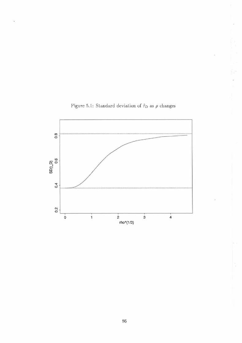
Figure 5.1: Standard deviation of î¿ as p changes
@o
qoo
_toU)
\fo
(\lo
430 2
rho^(1 /3)
86
Chapter 6
Cohort designs for two-treatment
crossover trials with one baseline
measurement
6.1 Introduction
In previous chapters, we showed that the average effect of treatment against baseline was
not estimable unless strong assumptions were made about the absence of period effects.
or the existence of a random effect for periods with known variance. In this chapter
we apply an alternative design which under some conditions enables us to estimate the
average effect of treatment against baseline. This alternative design is like an age-period-
cohort design, in that it supposes that periods correspond to the times of the year and
that some groups of subjects, referred to here as cohorts, entet the trial i','ith a delayed
start. In particular, we suppose that each successive cohort is delayed by exactly one
period. Provided we can assume that period effects are related to the time of year rather
than the length of time in the trial, referred to here as the 'age', this design will allow the
estimation of the average effect of treatment against baseline. Section 6.2 summarises
Age-Period-Cohort designs as they currently exist in the literature and illustrates the
association between these and our proposed 'cohort designs'. In Section 6.3 we build the
linear model for both the standard design used earlier and the new 'cohort design'. The
standard design with one baseline measurement taken before the first period treatment
is analysed in Section 6.4 and the corresponding cohort design with just two cohorts is
87

considered in Section 6.5. In Section 6.6 we discuss the treatment information for both
designs and in Section 6.7 we combine the treatment information in each stratum to
get estimates of the parameters of interest for the tlvo designs. The limiting cases ofo?rp : 3 -+ oo and zero are given in Section 6.8 and finally in Section 6.9 we make some
general conclusions about using cohort designs rather than standard designs.
6.2 Age-period-cohort design
The aim of this section is to give a general overvielv of age-period-cohort designs. Up
to now there are a lot of publications in which they attempted to show all features of
this design and to expiain all sorts of things on the basis of three variables, namely:
age, period and cohort which occrlpy a central position in cohort design. Based on our
literature review on some articles in this regard we can claim that the precise meaning
of the variables age, period and cohort, and thus also what is meant by age, period and
cohort effects, varies considerably from one study to another.
I(upper et al. (1983) discuss the specific problem of age-period-cohort analysis within
the general framework and give the following definition for age-period-cohort design:
"age-period-cohort analysis concerns methods for statistically analysing of such data
gathered on human population followed over time, the purpose of such analysis being
to quantify accurately patterns in the separate effects of age, period of time (e.g., as
measured by the year of occurrence), and cohort membership (".g., as measured by year
of birth)." Hagenaars (1978) in his paper gives the following definitions for these three
variables. He says that "in general it may be said that age is regarded as an indicator
for all the possible changes which are related to becoming older. Age can for example
be taken as an indicator for phenomena which are mainly of a biological nature, for
example becoming sexually mature, becoming tired more easily, getting ill more often."
For definition of period he says that "Period refers to all events which have taken place at
or between the moments of observation and which have influenced the phenomenon being
studies. Here too it will often be difficult to indicate exactly which event is responsible for
changes observed." Finally he defines cohort as "A collection of people born within thc
same period or a collection of people who have experienced a fundamental event during
the same period."
88
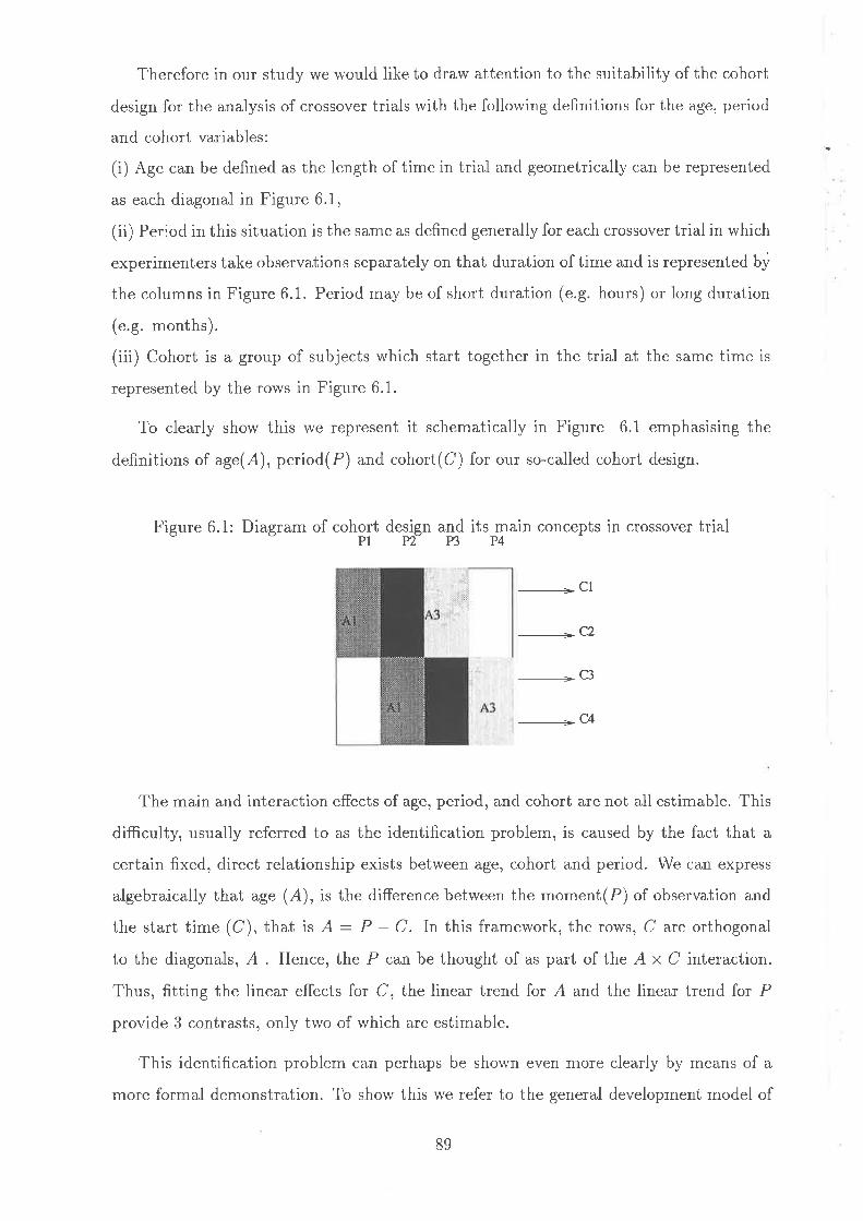
Therefore in our study we rvould like to draw attention to the suitability of the cohort
design for the analysis of crossover trials rvith the follorving definitions for the age, period
and cohort variables:
(i) Age can be defined as the length of time in trial and geometrically can be represented
as each diagonal in Figure 6.1,
(ii) Perìod in this situation is the same as defined generally for each crossover trial in which
experimenters take observations separately on that duration of time and is represented by
the columns in Figure 6.1. Period may be of short duration (e.g. hours) or long duration
(e.9. months).
(iii) Cohort is a group of subjects which start together in the trial at the same time is
represented by the rows in Figure 6.1.
To clearly show this we represent it schematically in Figure 6.1 emphasising the
definitions of age(A), period(P) and cohort(C) for our so-called cohort design.
Figure 6.1: Diagram of cohort design and its mP4
ain concepts in crossover trial
---------------- cl
+C2
-
c3
+c4
The main and interaction effects of age, period, and cohort are not a1l estimable. This
difficulty, usually referred to as the identification problem, is caused by the fact that a
certain fixed, direct relationship exists between age, cohort and period. We can express
algebraically that age (A), is the difference between the moment(P) of observation and
the start time (C), that is A: P - C. In this framework, the rows, C arc orthogonal
to the diagonals, A . Hence, the P can be thought of as part of the A x C interaction.
Thus, fitting the linear effects lor C, the linear trend for A and the linear trend for P
provide 3 contrasts, only two of which are estimable.
This identification problem can perhaps be shown even more clearly by rneans of a
more formal demonstration. To show this lve refer to the general development model of
89
Schaie (i965). He gives an additive model in rvhich each observation is seen as a rveighted
sum of the linear effects of the three independent variables
Y :boA+b"C IbrP
Since A: P - C it is also true that
Y : b"(P - C) + b"C + brP - (b" ¡ br)P + (b"- b,)C,
this can be reformulated as
y:eppIq"C.
In other words the additive model with three linear terms can be reduced to a model rvith
two linear terms which predicts exactly the same Y value as the three variable model.
Only two independent effect parameters are found to exist, that is, qo and q", from lvhich
it is no longer possible to deduce the three original coefficients bo,b",bp.
In our situation, we will be assuming that 'age' effects are not present, but that
'period' effects may be. This will only be appropriate in particular cases, such as asthma
trials where a subject's condition may be related quite strongly to the time of year in
which a treatment is applied.
The potential advantage of the baseline measurement in crossover trials is that it
enables estimation of the absolute effect of direct treatment by comparison rvith the
baseline. This advantage is lost if there are period effects present. The use of the cohort
design as described here is that the absolute effect of treatment may again be estimable,
even when period effects are present, provided age effects, as described, are not present.
For this to be successful, we require the following :
(i) Subjects enter according to a protocol so that no essential differences exist between
those subjects entering as the first or second cohort.
(ii) Length of time or experience of being in the trial does not influence the results. This
might not be satisfied, for example, if blood pressure is related to anxiety and the first
cohort is less anxious in period two than the second cohort. Different blood pressure
betlveen first and second cohorts at period two may then be partly due to anxiety level,
and hence related to what we have called here 'age' or time in trial.
The potential advantages of this design in crossover design are:
o it is useful when we suspect period effects (e.g. time of year), and
90

o we can estimate absolute effects of treatment and ca ryover
6.3 Building the model for standard and cohort de-
srgns
To shorv the efñciency of the cohort design lve compare it to the standard design of
crossover trial with baseline shorvn in Table 6.1. Here we use tn'o groups of subjects,
where each row represents a group of subjects, and each column represents one period.
In this situation, periods refer to the time a subject has been in the trial and to calendar
time.
Period
I 2 ,f
Group 1
2
A B
B A
Table 6.1: Two-treatment three-period crossover design with baseline measurements
Suppose, however, that subjects enter the trial at different times, as the trial pro-
gresses. It may be that we anticipate an effect related to the time of year in which the
measurement is made, but that we do not expect an effect related to the length of time
a subject has been in the trial.
To illustrate the idea, suppose that a study is undertaken as above, but with half
the subjects having a delayed entry at period 2 as shown in Table 6.2. ll there are 4n
subjects, this design would appear as shown in Table 6.2, with 2n subjects in each cohort,
and the subjects in each cohort being randomly allocated n to each of the two treatment
regimes. We note, for example, that a direct between-group comparison of treatment
with baseline is available in period 2 under certain conditions which we will explore in
the next section.
91

Period
1 2 ,f 4
1
2
3
4
Group
A B
B A
A B
B A
Table 6.2: Cohort design in two-treatment three-period crossover design with one baseline
measurement
In order to compare this with the standard design, it is convenient to present the
standard design in a similar way, with 4 groups of n subjects, as shown in Table 6.3.
Table 6.3: Two-treatment three-period crossover design with one baseline measurement
repeated as 4 groups of n.
Our purpose in this chapter is to compare the cohort design in Table 6.2 with the
corresponding standard design in Table 6.3. We assume that subject effects are random;
and that we have fixed effects for the period and mean ¡-1. The treatment parameters are
defined as:
o 16, the average effect of treatment; i.e. $¿ minus baseline;
. Ào,theaverageeffectof carryover; i.e. #.,fo, carryovereffects,minusbaseline;
o Zrp, the differencebetlveen A and B; i.e. rpfor A and -r¡ for B;
o 2)p, the difference in carryover between A and B; i.e. À¿ for ca ryover of A and
-À¡r for camyover of B.
Period
1 2 3
1
2
3
4
Group
A B
B A
A B
B A
92
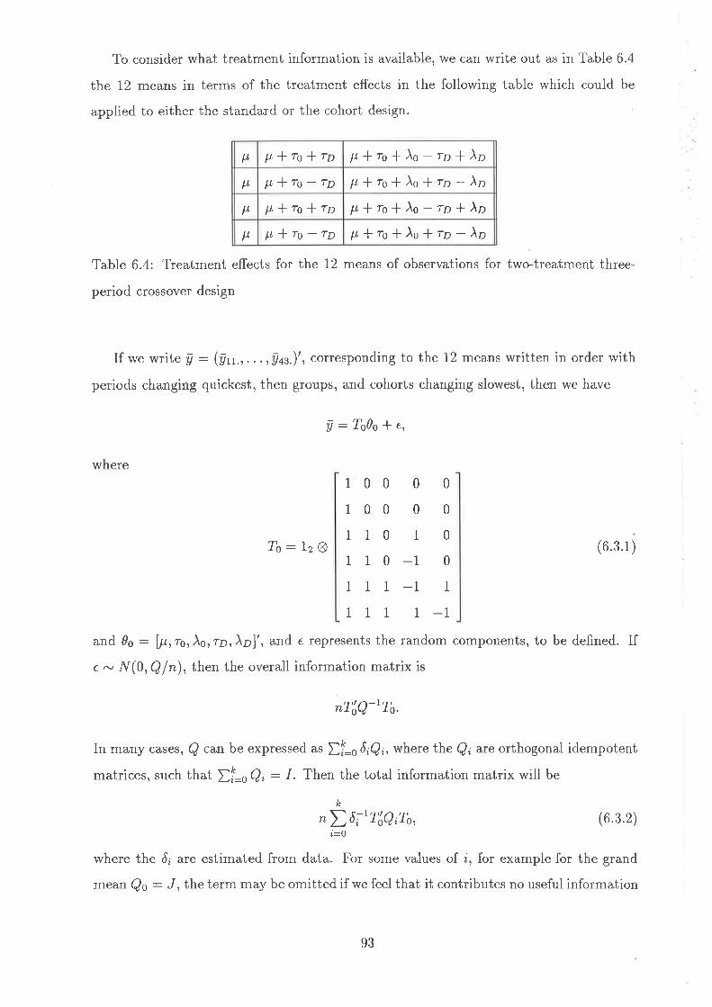
To consider what treatment information is available, we can write out as in Table 6.4
the 12 means in terms of the treatment effects in the following table which could be
applied to either the standard or the cohort design.
p lt+ro+rD p,*ro*Ào-rnlÀn
11 p,lro-ro þt lro*)o*rn-Ànp p+ro+rD p,*ro*Ào-ro*Ào
11 p,Iro-rn p,*ro*)o*rn-Ào
Table 6.4: Treatment effects for the 12 means of observations for two-treatment three-
period crossover design
If we write y : (Art.,. . . ,A¿s.)', corresponding to the 12 means written in order with
periods changing quickest, then groups, and cohorts changing slowest, then we have
a:To0o*e,
where
?o: 1z I
10101111i111
0000010-11 -111
0
0
0
0
1
1
(6.3.1)
and 06 : lpr10,Ào, rnrÀo]', and e represents the random components, to be defined. If
e - l/(0, Ql"), then the overall information matrix is
nTlQ-rTs.
In many cases, Q can be expressed as ff=o ô¿Q¿, where the Q¿ are orthogonal idempotent
matrices, such that Ðl=oQ¿: .[. Then the total information matrix will be
k
nl6;tr[e¿ro, (6.3.2)i=O
where the 6, are estimated from data. For some values of i, for example for the grand
mean Qo : J , the term may be omitted if we feel that it contributes no useful information
93
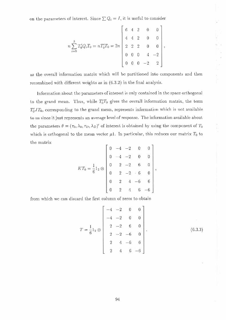
on the parameters of interest' Since DQ¿:1, it is useful to consider
642 0 0
0
0
2
2
nlf[qofo: nTåTo :2ni=0
442 0
222 0
000 4
000-2
as the overall information matrix which rvill be partitioned into components and then
recombined with different weights as in (6.3.2) in the final analysis.
Information about the parameters of interest is only contained in the space orthogonal
to the grand mean. Thus, while 4To gives the overall information matrix, the term
T¿JT¡, corresponding to the grand mean) represents information which is not available
to us since it just represents an average level of response. The information available about
the parameters d : (ro, Ào,rD,)¡)' of interest is obtained by using the component of Tq
which is orthogonal to the mean vector p,I. ln particular, this reduces our matrix Ts to
the matrix
Kro - år, *
1T: -1, R6 --
0-40-402020202
000060
-60-666-6
r)
-2-2-2
4
4
from which we can discard the first column of zeros to obtain
-4-4
2
2
2
2
2
2
2
2
4
4
0
0
6
6
6
6
0
0
0
0
6
6
(6.3.3)
94

Hence the available information about 0 : (ro, Ào,rD, À¡)' is contained in the information
matrix
.nT: n,T'T : -oJ
84 0
48 0
00 24
00 -12
0
0
-t212
(6.3.4)
This is the same for both standard and cohort designs. We want to look at T|Q;T,the
information contained in the ith stratum. This will be different for the standard and
cohort design.
However, we want to see where the treatment information goes, and holv much is lost
when we take out periods. We could do that by putting a term for periods in the model
and comparing joint information matrices for d with and without periods.
An alternative is to consider the projection matrix which takes out period effects and
see which part of Z ends up in that subspace. Thus, we are seeing Q as not just a variance
matrix, but rather as a way of splitting up t € ,R12 into separate components based on
the strata in the experiment, to see how much treatment information is lost into each
subspace. Later on we can make the choice as to which components we recombine to get
treatment estimates.
6.4 Standard design
We first look at describing the treatments effects for the 12 means contained in both
standard and cohort design defined in Section 6.3.
6.4.L Information matrices and parameter estimates
In the crossover design with baseline measurements described in Section 6.3 we assume
that we have means with expected values as shown in Table 6.4.
(I-J)y:T0te, (6.4.1)
(6.4.2)3
Q:Ð6oQ.i=l
rvhere e - l/(0, Qln) and
95

where Qt,: J 81(8,/ represents the projector matrix for Periods, Qr: (1S/A 1- "/8J Ø J) represents the projector matrix for Groups, and Q3 : (18 I{ Ø I - "/ 8If S /)represents the projector matrix for Periods x Groups, and the matrices in the l(ronecker
products are of dimension 2, 3 and 2, corresponding to Cohorts, Periods, and Groups
withinCohorts,respectively. Thecoefficients 6¿in(6.4.2) areô2:o2*3o!,fi:63:02,although d1 would also include a component relating to the variation between Periods.
Since it is unlikely that we would regard the periods as a random rather than a fixed
effect, we would not use ð1 in our recovery of treatment information.
We can think of the information on d as coming from the three different strata. Thus,
since ff=, Q¿: U - J), and since T'JT :0,,
r'r :f,''on''t=l
Hence, the information matrix for the ith stratum is T'Q¿T. These will be given in the
first column of Table 6.8.
The estimate of 0 from the ith stratum is
0¿: (T'Q¿T)-tr'Qny.
and these can be combined using
" - (P 6irT'8¿T)-'(Ð 6;IT'Q¿T0¿), (6.4.3)
provided suitable estimates of ô¿ are available. The cases i :0,1 correspond to the grand
mean and periods, respectively, and we will not attempt to recover information from
these strata. Hence the summation in (6.4.3) will be for i : 2,3 only.
6.4.2 Analysis of va-riance for standard design
For the standard design from equations (6.4.1) and (6.4.2), we can write out the table
of the analysis of variance for the standard design. We can write
vE(YY'):{Q¡nT00'T'},
where we have ignored terms involving the periods, from which lve can get the expected
sum of squares for each stratum as
n E {Y' Q ¿Y}
:'i,.-")!å r- -"ïrT r?;Tl}'
96

Since trace(Q¿) : rank(Q¿), then the expected mean squares are
EIVISI : ô; * nq'T'Q¿T0lrank(Q¿),
as shorvn in Table 6.5.
SSSource EMSDF'
Table 6.5: Analysis of variance for standard design
6.5 Cohort design
In the cohort design we have the same model (6.4.1) for the 12 means, and the matrix
Q still has the same covariance structure in terms of the between and within subject
effects. However, the projector matrix for Periods is now changed, because the 12 means
are now assigned to five different periods, rather than the original three. Furthermore,
Groups and Periods are not orthogonal. This implies that we cannot ìust use the Groups
stratum as it stands because it has some period effects in it. We can explore the different
strata by considering:
o Periods (ignoring Groups), with 3 degrees of freedom,
o Groups(ignoring Periods), with 3 degrees of freedom, and
o the Group x Period interaction, with 5 degrees of freedom.
The first two of these can be examined by considering the following contrasts. Contrasts
on Groups can be expressed as the row contrasts 91, 92 and !3:
LlQØJØJ)gGrand Mean
Periods
Groups
Period x Group
Subject within Groups
(Subject within Group) x Period
na'Qta
na'QzY
na'QsY
o2 ¡ Jo! j no'T'Q2To lJo2 + no'T'q3ro 16
o2 + 3ol
o2
2
J
6
4(rz - 1)
8(n - 1)
lZnTotal
97

1 -1 -1
1 -1 1
I 1 1
1 I 1
1 1 1
1 1 1
-1 1 1
1 1 1
-i i 1
1 I I
1 1 1
i -1 -1
9z
from which a projector matrix for Groups (ignoring Periods) can be formed as
3
ec : Ð gngil@'ngo)i=l
Similarly, contrasts for Periods are the column contrasts pt, pz and p3
9z9t
0 -1 1
0 -1 1
-1 1 0
-1 1 0
-2 1 1
-2 1 1
1 1.t
1 1 ,
(6.5.1)
(6.5.2)
(6.5.3)
Pz
and the projector matrix for Periods (ignoring Groups) can be given as
3
ep:løn;l@,;vò.i=l
PzPt
Due to the fact that groups and periods here are not orthogonal, QçQ, t 0. We can
identify the relationships between the six contrasts by the following matrix of cross-
products. If we let W : (gt,,gz,gs¡Pt,,Pz,ps), then
W,W
t2
0
0
0
0
4
0
t2
0
0
0
0
0
0
0
0
24
0
4
0
0
0
0
4
0000t20080000
which shows the lack of orthogonality between groups and periods because g'Lh + 0.
This selection of contrasts is such that:
. (gz,gs) capture differences between groups within cohorts and are orthogonal to periods,
. (pr,pz) capture differences between periods which are orthogonal to groups, and
-1 0 0
1 0 0
0 0 1
0 0 1
98

o 91, the difference betrveen cohorts,, is not orthogonal to p3, the contrast between the
first and last period.
The implication is that 2 degrees of freedom for groups (ignoring periods), correspond-
ing to !2 and !s, a,re the same whether we fit groups before periods or periods before
groups. Similarly, 2 degrees of freedom for periods (ignoring groups), corresponding to p1
and pz, are the same whether we fit periods first or second. The only difference between
the two analyses arises from the order of fitting g¡ and p3.
If we fit groups and periods together, the projector matrix is
Qcp : w(w'w)-rw', (6.5.4)
and, since all these columns are contrasts and hence l'W :0, the projector matrix for
the interaction stratum is
Qnt:K-Qcr.
Figure 6.2 shows the relationship between the vectors produced using these projector
matrices. Thus, if we consider a vector Qcpy, as the projection of the vector y onto the
space of Groups and Periods, in a case when the Groups and Periods are not orthogonai
to one another, then the vector can be decomposed in two distinct \¡/ays. The first of
these has a component in the Groups space, Qçy, and a remainder, QA7A, in the Periods
(eliminating Groups) space. The second has a component in the Periods space, Qpy, and
a remainder, QcpU, in the Groups (eliminating Periods) space.
Figure 6.2: The relationship of projector matrices in cohort design
". Q
",rY
We can obtain Qçp directly, or we can obtain it by orthogonalizing the columns of
I4l. This is conveniently done in one of two ways:
acpi
a prcY
Q^yU
Groups
99
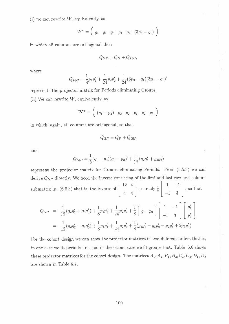
(i) rve can rewrite W, equivalently, as
in which all columns are orthogonal then
W*: 9t 9z 9s Pt 'Pz (3Pt - gr)
Qcp: Qc -l Qeg,
where
Q rp : rrnrr\ + )nrn, + f,n;,nr-
gr )(3ps - gr)'
represents the projector matrix for Periods eliminating Groups.
(ii) We can rewrite W, equivalently, as
¡y+ (gt - p") 9z 9s Pt Pz Ps
in which, again,, all columns are orthogonal, so that
Qcp:QpiQclp
and
Qqe: å,n, - pz)(gt - p")' + |krsl+ grgL)
represent the projector matrix for Groups eliminating Periods. From (6.5.3) we can
derive Qcp directly. We need the inverse consisting of the first and last row and column
Itz4l lr -rIsubmatrixin (6.5.3) thatis,theinverseof | - l,namelyl I l,so that
lt 4)' "'l-r 3l'
ecp : |ø,n;+gssL)+fn,ri +fin,n*ål* -]ll, ;tll;; llr 1 I l'
¡rezn'z+ g"gL) + intri + finrnL+ ,kts't - etP's- pssi + 3pspå)
For the cohort design we can show the projector matrices in two different orders that is,
in one case we fit periods first and in the second case we fit groups first. Table 6.6 shows
these projector matrices for the cohort design. The matrices 41, Az, Br, Br,CrrC2, D1, D2
are shown in Table 6.7.
100

Cohort Design (Groups first)Projector Matrix Cohort Design (Periods first)
)ø*t1
B2
B
,4,
Ai
A2
AiØJzQp: äPeriods
tI
aGPIC Cr,
1
24
Ct CzQc: I{4Ø J3
l.,t\bGroups
Qn:frInteraction
(A 1 represents A1 transposed about the reverse diagonal; that is, about the diagonal
running from bottom left to top right of the matrix.)
Table 6.6: Projector matrices for cohort design for two orders of fitting
A I
5
-1
-1
1
2
1
1
1
2
Az:-1
2
-1
I
I
2
I
1
1
Bt:8
4
4
-4 4
I
5
b
-1
B
0 003-30
-3 304
-44
-44
-4
-4 4
4
,7I
1
I
1
-44
-1I
-1I
4
-47
-1I
-1
-44
4
4
4
4
4
1
7
1
I
CI
0
0
-ð
-3-3-.t
0
0
3
3
rt
ù
0
0
,)
3
.)
.)
0
0
-3-3-3-,)
0
0
0
0
0
0
0
0
0
0
0
0
Cz:
Dt:
8
-8-4
4
-44
-88
4
-44
-4
-44
11
-5-I
1
4
-4-511
1
-7
-44
-7I
11
-5
4
-41
-7-511
Dz:
0
0
3
3
11
.)
0
0
t)
r1
3
rtr)
0
0
,f
3
3
ó
0
0
t)
,f
3
,)
0
0
0
0
0
0
0
0
0
0
0
0
Table 6.7: Matrices introduced in the table of projector matrices for cohort design
101
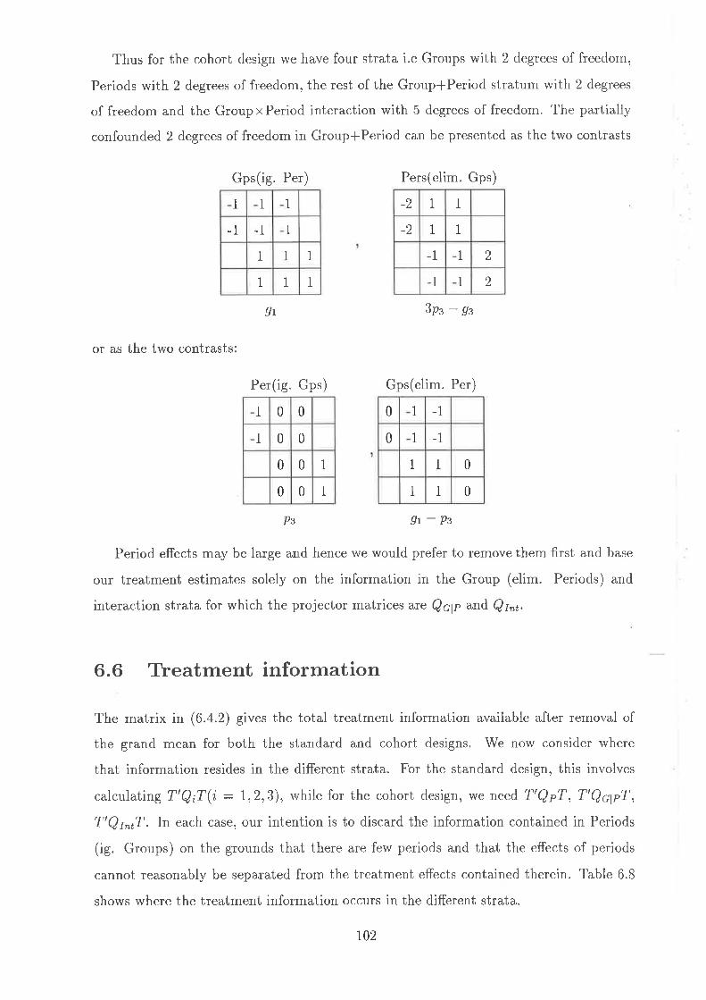
Thus for the cohort design lve have four strata i.e Groups with 2 degrees of freedom,
Periods with 2 degrees of freedom, the rest of the Group{Period stratum with 2 degrees
of freedom and the GroupxPeriod interaction with 5 degrees of freedom. The partially
confounded 2 degrees of freedom in Groupf Period can be presented as the two contrasts
Gps(ig. Per) Pers(elim. Gps)
a,1 1
o 1 I
-1 1 2
-1 1 2
9t 3pz - gz
or as the two contrasts:
Per(ig. Gps) Gps(elim. Per)
Pz 9t-Pz
Period effects may be large and hence we would prefer to remove them first and base
our treatment estimates solely on the information in the Group (elim. Periods) and
interaction strata for which the projector matrices are Qclr and Qm.
6.6 Tleatment information
The matrix in (6.4.2) gives the total treatment information available after removal of
the grand mean for both the standard and cohort designs. We now consider where
that information resides in the different strata. For the standard design, this involves
calculating T']iT(i:1,2,3), while for the cohort design, we need T'QpT,T'QclpT,
T'QnT. In each case, our intention is to discard the information contained in Periods
(ig. Groups) on the grounds that there are few periods and that the effects of periods
cannot reasonably be separated from the treatment effects contained therein. Table 6.8
shows where the treatment information occurs in the different strata.
1 1 1
-1 1 1
1 1 I
1 1 1
1 0 0
1 0 0
0 0 I
0 0 1
0 i -1
0 1 -1
1 1 0
1 1 0
r02
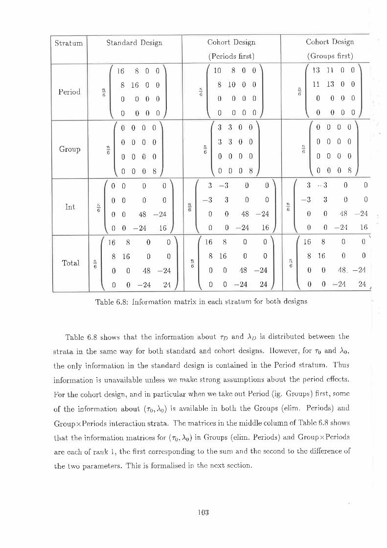
Cohort Design
(Groups first)
000000000008
n6
0
0
0
0
6
ù
-t)
0
0
-ù3
0
0
0
0
48
24
0
0
-2416
n6
16
8
0
0
8
16
0
0
0000
48. -2424 24
Table 6.8: Information matrix in each stratum for both designs
Table 6.8 shows that the information about rp arrd )p is distributed between the
strata in the same way for both standard and cohort designs. However,, for rs and Às,
the only information in the standard design is contained in the Period stratum. Thus
information is unavailable unless we make strong assumptions about the period effects.
For the cohort design, and in particular when we take out Period (ig. Groups) first, some
of the information about (to, Ào) is available in both the Groups (elim. Periods) and
Group x Periods interaction strata. The matrices in the middle column of Table 6.8 shows
that the information matricesfor (16,À¡) in Groups (elim. Periods) and GroupxPeriods
are each of rank 1, the first corresponding to the sum and the second to the difference of
the two parameters. This is formalised in the next section.
Cohort Design
(Periods first)
Standard DesignStratum
10
8
0
0
8001000000000
b
13
11
0
0
11 0 0
1300000000
n6
16
8
0
0
8001600000000
6Period
J
ù
0
0
6
300300000008
Group
0
0
0
0
n6
000000000008
ù
t)
0
0
ù
,f
0
0
0
0
48
24
0
0
24
16
Int
0
0
0
0
00000480 -24
0
0
24
16
6
16
8
0
0
8
16
0
0
0
0
48
24
0
0
24
24
n6Total
16
8
0
0
801600480 -24
0
0
24
24
n6
103
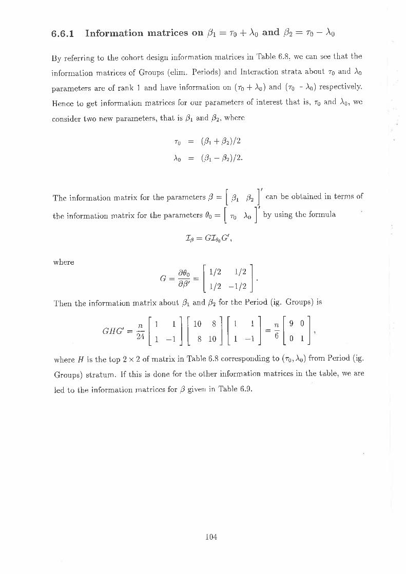
6.6.1 Information matrices on þt - ro * Ào and B2: ro - Ào
By referring to the cohort design information matrices in Table 6.8, we can see that the
information matrices of Groups (elim. Periods) and Interaction strata about rs and )s
parameters are of rank 1 and have information on (rs * )o) and (16 - )o) respectively.
Hence to get information matrices for our parameters of interest that is,' rs and Àe, lve
consider two new parameters, that is B1 and B2, where
rs : (0, + 0r) 12
)o : (þ' - þr) 12.
The information matrix for the parameters þ :
the information matrix for the parameters ds :0, can be obtained in terms of
)o by using the formula
p
Tg
l
t'
Ip: GIeoG',
where
G:ffi:1,,,,7
":)Then the information matrix about Ér and 0z for the Period (ig. Groups) is
1
rl[':,:]ll1 n
6
9001
GHG' : +n 1 i
where 11 is the top 2 x 2 of matrix in Table 6.8 corresponding to (rs, À¡) from Period (ig.
Groups) stratum. If this is done for the other information matrices in the table, we a e
led to the information matrices for B given in Table 6.9.
104

(t)
+ H 5 (t)
H Ê-
stj n a- t o (t oq H
l\o !i äo4
o N\J
9(h ;oc
).-
: Ô
!l ^
cn=
+U
H
H =o
-=Ø
óoe H
FÚ n ô a- o)lJ
o r.
9
ÀO
\\/
ollJ
O
olJ
O
O¡.
o
H o O Ó)l¡ O
H c+ o 4 P c+ H O ôl¡
C¡:
O
o)lÈ
C/9
O
ll -+ ôls
O
ì.O
ÈO o)
lË
O
t.9
o)15
ot9
È p o i^ H n H H o H p c+ n X Þ.) H $ N Ø H p -l t- H 4 <t o a) oc H Ø
H Ð Èa
F< + 4 ol + o ol I
b.9
CJro E a- (t ûc !r _
,¿
H Ø -¡ cJr
ts (t o H H tu H ê- Ø b.9
CJr O
H o tst o -l- { crr
ôrl
HO o-;
i;O oc
o H o o c+ p ûc o +) n H + H H - o p o cn H 9.)
c+ H p ct ol _l_ I p H p- ol I o * o' 4 c+
OJ o) ie { o r.t o Ø + o el-
r-i o p + t{ o c+ Ð E p el- o a-
,
C,I

two parts of the parameters of interest lies. By referring to Section 6.5 we can say that
Groups (elim. Periods) stratum can be d.ecomposed into two substrata as Groups within
Cohorts vr'ith the projector
(fis,d,+ l nú),
with 2 degrees of freedom and ô2 : o2 I3o,2 and the one degree of freedom for Cohorts
(elim. Periods) with the projector hdd', where d: (gt -ps). We need to establish the
appropriate variance to use for the contrast d. The projector matrix corresponding to
this contrast is d(d'd)-td' to that the sum of squares for this stratum is
S Sc"p : a, d(d, d)-, d,, y : fi@, r),
: r1{a, ù)r,
and the expected sum of squares ignoring the treatment effects
E (S S c "ù : ltror" E (d'' yy',1).
Now we know that
var(y) : o'(t Ø K) + (o" + 3o!)(K Ø J) (6.6.1)
: 02I +zo!(I Ø J) - o2J
: o'(I - J) +Jo!(I I "/),
and we can show that d'(I - J)d,: ô : 8 and d'(I Ø J)d, :16/3. It follows that, ignoring
treatments for the moment,
E(S Sc"P) : o2 ¡ 2o2" '
The contrasts 92 and 93 form the Group within Cohort stratum with two degrees of
freedom and they provide the sum of squares
1
S Sc,c : fitrace{g'2yy'gz
+ gLay'gt},
for which the expected mean square can be expressed, using (6.6.2), as
E(M SG.c) : h*r*rÐlr'g'n| - J)go + 3o'?,si| Ø J)g¿lj.
Now we have
g'¿(I - J)gn : 12, g'i] Ø J)g¿ : L2
for i : 2,3,, so that, ignoring the treatment effects again, we obtain
E(M Sc-c) : o' -f 3o!'
So to get 0, we have the following Table 6.11.
106

Stratum Parameter estimable degree of freedom IVISE
Cohort (elim. Periods) (to, Ào) I o2 +2o?
Group within Cohort (rr, Àn) 2 o2 ¡ 3o2,
Interaction (to, À0, ,o, Àn) 5 o 2
Table 6.11: Those strata which contribute to estimate some parameters of interest
6.7 Combining information
The parameter estimates in (6.4.3) can now be obtained by combining the information
from these three strata. The pair (â0, io) and the pair (â¡, ¿) ut" uncorrelated with
each other in all strata, and hence lve can look at their estimates separately. Information
about ("o, )o) is available in two strata, with weights o2 and (o2 +2o2,), while information
about (rn,Àn) is available with weights o2 and (o'+ 3øl). trstimates of o2 and o! arc
obtained from the appropriate residual lines in the analysis of variance in Table 6.5, these
being calculated in exactly the same way for both the standard and cohort design.
6.7.L Estimation of ("0, Ào) in cohort design only
For the average effect of treatments, that is (16, )s), we can obtain estimates from each
of the Group (elim. Periods) and the interaction strata, as shown in the middle columns
of Table 6.12, and then combine them with appropriate weights using:
âo
io I ]) '
ri{Q"t'+ (1 + 2p)Q'^'}v'{l:3
o.)
(1+rJ
.)
ri(Q.tr+(1 +2p)Qm,)a,(r + 2p)
r*pp
1
where Zr is a submatrix of matrix 7 given by the first two columns in (6.3.3), corre-
sponding to the pair of parameters (rs, Às). This leads to the contrasts represented in
the last column of Table 6.12. The covariance matrix of these combined estimates is
fr o2 7*pp
p
1*pn
r07
(6.7.1)

Cohort design
Estimator Periods
(ig. Groups)
Groups
(elim. Periods)
Interaction Combined
7g1
-4r2-4t2
t2-2t2-2
36
0
0
II
II
-9-90-9-90
0 9-90 9-9
-9 90-9 90
It
010010
-1 00100
)o
2
2
2-l-2 I
-2 -1 4
q t4
1
099099
-9 -9 0
-9 -9 0
0-9 I0-9 I
9-909-90
1t
00100 i
0
0
-1 0
-1 0
Table 6.i2: Contrasts for estimating parameters in cohort design
Table 6.13: Contrasts for estimating parameters in standard design
Estimator Period
Standard Design
Group Interaction Combined
Tg4
i I
I
0
0-1
-1 10110
None None None
)o None None
0
0
-1
-1
1
1
0-1 1
0 I 1
None
108
Nolv lve can have a look in each stratum at the contrasts for the tlvo designs and
compare them. First, for the standard design, we have the results shown in Table 6.13.
Holvever, these results are not useful, because all information about the tlvo parameters
are in the Period stratum and in the presence of strong or unknolvn period effects, we
cannot estimate the average effects of treatments. In fact this information in the Period
stratum oî 16 and )s in Table 6.13 is not available when we suspect period effects. The
cohort design offers a way to get more useful information for average effects of treatments.
6.7.2 Estimation of (ro,Ào) in both designs
Table 6.8 shows that the information about (ro,Ào) is in Groups (elim. Periods) and
the Interaction strata, for both standard and cohort designs. If we put p: o?1o2, then
combined estimates can then be found as
ï ] I' "{Q'1'+ (r + rp)Q'^'\ u
)r,ro"o+ (1 + rp)e,^,) y,
0
8+(1+3p)
48
-24
1
4(r + p)
(r+2p)10+3p) 1
I2
where T2is a submatrix of matrix ? given by the last two columns of (6.3.3) corresponding
to the pair of parameters (r¡, )¡). This leads to two contrasts which should be applied
to the vector y, and these may be represented by:
1
4(1 + p)
1
îp
_p (1 +p)
p _(1 +p)
0
0
p (1 +p)
p _(1 +p)
0
0
-2p (1 + p)
2p -(1 + p)
(1 +p)_(t + p)
-2p (1 + p)
2p -(1 + p)
(1 +p)_(1 + p)
)r:4(1 + p)
109

o, rlr+ze r*rp I rc.7.2)E,:4n(t+p)|,*,o 2(1 +rol l
Except for the change in the definition of n, these estimates and their covariance matrix
agree rvith the results of Section 3.3.1.
The covariance matrix of these estimates is
for which the estimates are:
6.7.3 Estimates of treatment effect minus baseline
We might want to look at estimates of r¡ - p and rn - þ where ¡-r, is the baseline
measurement. The estimates of (to, Ào) and (rp, Àp) are uncorrelated, and hence the
covariance matrices of 0 canbe found in (6.7.1) and (6.7.2). As we defined our parameters
in Section 6.3 we have
re- þ
rn-F
Àt-tl
Àp-þ
(6.7.3)
/^^\If we put f' : ( O, -p în - tt \¡ - tt \a - tt ), then to get the estimates and
covariance matrix of new vector ri from (6.7.3) we can write
: ro*rn
: To-TD
: ,Ào*À¿
: )o-Ào
0100-1 0
1011 0-1
1
1
0
0
îo
io
'tD
iD
0F
1
-p 3(1 + p) 0
p r-l p 0
-(2 + 3p) l*p 0
_(2 + p) _(1 + p) 0
rt- þ 4(1 + p)
110
TB - l-t
1
4(t + p)
\o- t'1
1
4(r + p)
Àn-tt4(r + p)
These four contrasts should be applied to the vector of means y to estimate the effects
The covariance matrix of 17 can be obtained by using the fact that
Var(f¡) - Ði: FÐ,7',
which gives
5+10p+4pt
3*6p+4p2
1-l7p+4p2
-1 + p*4p2
3*6p+4p2
5*10p+4p"
-1 + p l4p'1*7p+4p'
r+7p+4p'
-l+ p+4p2
6*I4p+4p'2+2p+4p2
-lI p+4p'
l-l7p+4p2
2*2p+4p'6 -f l4p + 4p2
6.8 Limiting estimates in terms of p
In this section we consider the estimates of the parameter of interest when p tends to
zero and infinity.
6.8.1 The estimates and covarÍance matrix when p -+ æ
I1 p -+ oo, that is rvhen o? -+ oo, the subjects are considered as fixed effects and we
obtain the follorving estimates of r¡ and )¡:
0p r* p
-p 3(1 + p) 0
_(2 + p) _(1 + p) 0
rlp 0-(2 + 3p)
-2p r* p 3(1 + p)
r-lp2p _(1 + p)
-2p _(1 + p) Lrp_3(1 + p) _(1 + p)2p
2p _(1 + p) r*p-2p r-lp 3(1 + p)
2p -B(1 + p) _(1 + p)
-2p _(1 + p) l-lp
111

I-1 1 0
1 10-1 1 0
1-1 0
-2 112 1 -1
-2i12-l-1
î'o
Ào
These estimates are orthogonal to both Groups and Periods, and are those estimates
obtained solely from the Interaction stratum in Table 6.8.
Because the estimates of rs and Às are independent of p, then those estimates do
not change when p changes. The covariance matrix of estimators however, tends to
infinity when p -+ æ because the contrasts involve comparisons between as well as
within subjects. For 17, the cohort design gives the estimates:
î,q - tt
rn-þ
1
4
1
4
1
4
À,q- pI2
o 1 3
2 1 I
-2 -i 1
2 -3 -1
1 ù 0
1 1 0
-3 1 0
1 -1 0
1 1 0
1 ,) 0
-1 I 0
-.) I 0
ll2

i,
All elements of the covariance matrix for 17 in this case become large as p -+ oo
because the estimates are not orthogonal to subjects.
6.8.2 Estimates and their covariance l¡vhen p + 0
In this subsection we consider the estimates and their covariance when p 4 0, or in other
words when there is no difference between the subjects. Since the estimate of the pair
(ro,Ào) isindependentof pthenitremainsthesame,butforthepair (rn,Ào) wehave
tt1
2
2 I 1
o 1 .)
2 -3 -1q
-1 1
TD
i,
I
1
4
0
0
1 1
1 1
0
0
111 -1
The covariance matrix of d is
02limXr: -p-+o ' 4n,
4 0 0 0
040000110 012
The result in this case for 4 is given below and shows that the estimates are orthogonal
to Periods, but not to subjects:
0
0
10-1 0
0
0
10-1 0
113

î,a, - p
rn-þ
\-.un
I4
1
4
À¿, - tt
\"-t'
The covariance matrix for 17 in this case is
1
2
0 1O,)
0 1 1
0 1 1
0 -r) -1
5 3 I -13 5 -1 1
1-1 62-1 126
1
oolimp-+o 4n
6.9 Conclusion
By using the cohort design in crossover design, we can recover some information about
(to, )o) and obtain estimates for them within and between subjects. This method opens
the way for a more detailed examination of the topic.
It has been shown that the block effects corresponding to Cohorts and Periods are not
orthogonal to one another. This lvill also be true in more general cases. The resolution of
this in general requires the application of the results of James & Wilkinson (1971) which
0 .) 0
0 1 0
-2 1 0
-2 1 0
0 1 0
0 3 0
-2 -1 0
-2 I 0
0 -1 1
0 I J
0 -3 -10 1 1
t74

allorvs the appropriate partitioning of these spaces. Although the original worl< of James
& Wilkinson (1971) is concerned rvith Blocks and Treatments, rve apply it to a situation
rvith tlvo nonorthogonal blocking factors.
115

Chapter 7
Block structure of cohort desrgns
7.L Introduction
In the previous Chapter, we considered a particular example of a cohort design in which
a second cohort was delayed by one period. It was shown that treatment information
was available in the Cohort (elim. Periods) and Interaction strata.
We will now compare a variety of such designs with the corresponding standard design
in which subsequent cohorts do not have delayed entry.
In cohort designs two basic types of structures are the block structure of the experi-
ment and the treatment structure. The purpose of this chapter is to present an analysis
of the block structure of the general class of cohort designs. We will consider the general
case where each of c cohorts are observed for p periods, but with each successive cohort
entering the study after a delay of one period. Thus, the experiment will occur over a
total of (p + " - 1) periods. Within each cohort we will assume there are g groups of
n subjects, where each subject within a group receives the same treatment regime. We
will show the ANOVA tables for the standard and the cohort designs with a data vector
of length cpgn in terms of the block structure, where g is the number of groups in each
cohort and n is the number of subjects in each group. We show that the differences
between them are only due to differing idempotent matrices for cohort,, periods and the
interaction.
We use the work of James & Wilkinson (1971), because James and Wilkinson's ge-
ometrical formulation provides a way of looking at the , , (p t c - 1) array of means
a
116

and identifying the contrasts for Cohort(elim. Periods) and their expected mean squares.
For this purpose we need to split the contrasts for Cohort(elim. Periods) into different
1 degree of freedom contrasts each lvith a possibly different expected mean square and
then to identify the projector matrix for projecting onto the vector space spanned by the
columns of Cohort(elim. Periods). We then consider several examples in detail. In a
special study we have got the orthogonal contrasts for the three strata for two and three
cohort designs with up to 7 periods in each cohort. For these special cases we obtain the
analysis of variance table in Section 7.3 and by using a function which we have written in
S-PLUS (Venables & Rezaei (1996)) we show their projector matrices and the expected
mean square for each stratum.
7.2 Cohort design in general
The design and analysis of cohort designs for the two-treatment three-period design with
one baseline measurement is carried out in the previous chapter. In that design, it was
found that there was nonorthogonality between periods and cohorts, and this led to using
the Cohort (elim. Periods) sum of squares to provide some of the treatment information.
In this section, we shall describe the block structure of a general cohort clesign and
our response will be supposed a linear function of parameters with a covariance matrix
whose spectral form is governed by the blocking arrangement. The model has c cohorts,
p periods in each cohort where each successive cohort starts one period later than the
previous one, such that the design has a total of pl c- 1 periods. Within each cohort we
have g groups and within each group there are n subjects. These groups will eventually
each be assigned a different treatment regime, but the analysis in this Section will rely
on the fact that the ng subjects in a cohort are randomly allocated to these groups. The
design is shown in the following layout in Figure 7.1.
I17

Figure 7.1: Fu1l cohort design length cpgn
I
p
I
1
c
2o
c
Ic-1
g
c
g
p+c-1
In this and subsequent tables, we suppose that the data are written in standard
order, running over the last subscript first, where the data values are given as U¿jtt.,
for the ith cohort (ó: I,2,...,c), jth period (j :I,2,...,p), kth group in ith cohort
(k : 1,2,.. . ,g), and /th subject in kth group (l : I,2,. .. ,n). Data from the experiment
will be denoted by y, an cpgnx 1 column vector, with mean E(y) and variance-covariance
matrix Q
We consider a model which can be represented as
U¿it t : tt * l¿ * r¡ I þ;m I r7jkq + eiikt (7.2.r)
where þ, 1¿ and zrj are the grand mean, ith cohort, jth period effect respectively, and B¿¡,¡
is subject effect from the /th subject in kth group in ith cohort and rç¡nt¡ at this stage
is used to describe the set of treatment effects applied to the /th subject in kth group in
jth period in ith cohort. In this model, the þ¿m are independent random variables which
are normally distributed with mean 0 and variance o! and are independent of the e¿¡¡¡
which are independent random normal variables with mean 0 and variance o2.
118
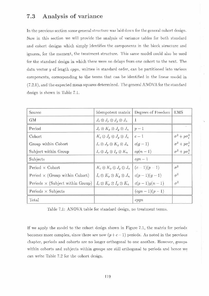
7.3 Analysis of variance
In the previous section some general structure was laid dolvn for the general cohort design.
Now in this section rve lvill provide the analysis of variance tables for both standard
and cohort designs which simply identifies the components in the block structure and
ignores, for the moment, the treatment structure. This same model could also be used
for the standard design in which there were no delays from one cohort to the next. The
data vector y of length cpgn, written in standard order, can be partitioned into various
components, corresponding to the terms that can be identified in the linear model in
(7.2.1), and the expected mean squares determined. The general ANOVA for the standard
design is shown in Table 7.1.
Table 7.1: ANOVA table for standard design, no treatment terms
If we apply the model to the cohort design shown in Figure 7.1, the matrix for periods
becomes more complex, since there are now (p+ "- 1) periods. As noted in the previous
chapter, periods and cohorts are no longer orthogonal to one another. However, groups
within cohorts and subjects within groups are still orthogonal to periods and hence we
can rvrite Table 7.2 lor the cohort design.
Source Idempotent matrix Degrees of Freedom trMS
GM J.ØJpE)JsØJ" 1
Period J"ØKpØJsØJ" p-1.
Cohort
Group within Cohort
Subject within Group
K"ØJpØJsØJ"
I"ØJPE)KgØJ"
I"ØJpE)IsØK"
c-l
"(g - 1)
cs(n - 7)
o'+ po?
o'+ po?
o, + po?
Subjects cgn-I
Period x Cohort
Period x (Group within Cohort)
Periods x (Subject within Group)
I("ØKeØJsØJ"
I"Ø I{e Ø Ks Ø J"
I"Ø KpØ IsØ K"
(c-1)(p-1)c(p-lxg-t)c(p-1)e(n-1)
)o
02
o2
Periods x Subjects ("gr- tXp- t)
Total cpgn
119

Source Idempotent matrix Degrees of Freedom EMS
GIVT J"ØJpØJsØJ" 1
Periods (ig. Cohort) StØJgØJ" P*c-2Cohorts (elim. periods)
Group rvithin Cohort
Subject within Group
s,&J^ñ¿I"ØJpgI(eg"I"I"ØJpØIsØK"
c-Ic(g - 1)
cs(n - I)o
o
'+po?
'+po?Subjects cgn-l
Period x Cohort
Period x (Group within Cohort)
Periods x (Subject within Group)
S¡8Js8"f"I"Ø KeØ I(s Ø J"
IcØI(eØIsØI("
(r-1)(p-z)c(p-r)(s-t)c(p-1)s(n-I)
o t
o2
o2
Periodsx Subjects ("sn- t)(p- 1) - (c- 1)
Total cpgn
Table 7.2: ANOVA table for general cohort design, no treatments term
In Table 7.2 we consider the projector matrix which takes out Period effects from the
mcdel and then consider a stratum named Cohort (elim. Periods) which is orthogonal
to Periods (ig. Cohort) stratum. As we can see, many lines in Tables 7.1 and 7.2 are
the same. The differences occur only in Periods (ig. Cohort), Cohort (elim. Periods)
and Periods x Cohort interaction. For these three lines, the idempotent matrices always
end in Js Ø Jn, indicating that we can average over all subjects within a cohort. Thus,
to get a block structure for the general cohort design we need only consider the vector of
(Cohort x Period) meansof length cp. InTableT.2,Sl,,92andSsareprojectormatrices
for Period (ig. Cohort), Cohort (elim. Periods) and PeriodxCohort interaction applied
in each case to the vector of Cohort x Period means of length cp. These throe projector
matrices add together to giveidempotent matrix (I - J) of dimension (cp- 1). Wewill
sholv how these can be presented in the next section.
7.4 Fitting periods and cohorts
We nolv consider just the table of Cohort x Period means with length cp, as shown in
Figure 7.2. Considering this in standard order across the rows, we get the model
y : [rl * Pn -f Cl * Tr I e, (7.4.1)
t20

where Zr considers lvhatever treatments are applied and e indicates the random effects
due to subject and error. In this case, each mean will nolv have a variance of (o2 -f o!) I gn,
with observations in the same cohort having covariance "?lg".We rvill ignore the factor
gn in this section, for convenience, and regard each value as a single observation rather
than as a mean of gn values. The variance-covariance matrix of e can then be lvritten
Var(e): o2(1"Ø Kp) * (o'+ p"?)U.Ø Jr).
Figure 7.2: Full cohort design, length cp
+ P----------------
1p
2
c
c-1
c
plc-1
For the Cohort x Period table of means we can identify the components in the block
structure. This will provide five strata whose orthogonai projector matrices can be shown
in the following;
. ./" 8 Jr lor gland mean;
o ,9s : K"Ø Jp for Cohorts ignoring periods;
r 51 : P(P'P)- P' - J for Periods ignoring Cohorts;
o 52 : X(X'X)- Xt - P(P'P)-P' for Cohort eliminating periods;
. Ss : I - X(X'X)- X' for Interaction stratum;
rlwhere r: lP : C ). Notethat C:1"81o, and (X'X) is singularwithrankof
(p+2"- 3). In this formulation, the .9; determine the block structure of the cohort design
1.21
experiment and with respect to the usual Euclidean norm divide R"p into subspaces
called strata. We can think of the columns of C and P as generating subspa,ces of R"p
withdimensionc-1andp+c-2respectively,andcorrespondingidempotentmatrices
So : I{"8,,I0 and Sr, after removing the grand mean. These subspaces are not orthogonal
to each other. To explore the relationship between these subspaces, we turn to the results
of James & Wilkinson (1971).
7.5 James and Wilkinson theorem
In the following section we summarise a geometrical approach to the analysis of nonorthog-
onal designs generated by projection matrices which was initially worked out by James &
Wilkinson (1971). Such a geometrical approach has quite general application to problems
in experimental design. In our cohort design, due to the nonorthogonality of two strata
in the design, we need to use the result of the above mentioned paper.
James and Wilkinson show that, if the projector matrices onto the spaces U and V.
with dimension (q,*),such that e ) nù, are U and V then there exist spaces
UtrUzr.. . rUkrUk+t,
Vt,Vzr., ,,Vk,
and the projector matrices
Ut,Uz, . . . ,UnrUt+,
VtrVzr... rVk,
such that rank(tJ¿) : rank(V) : r¿, D!=tri : rn and lfjl ri : et such Lirat,
U¡V¡ : 0 (i+i), (7'5'1)
U¿U¡ : 0 (i+i),V¿V¡ : 0 (i+i),
U¿VU¿ : p;Ur, (7.5.2)
VU¿V
rvhere 7t pr >...and if a¿ is such that cos2 aà: pi,t then a¿ is the angle between the projectionU¿y of any
r22
vector into U¿ and the projection l/¿y of that same vector into V¿. Nolv in the next section
lve show holv lve can get these pi's as the canonical correlation coefficients betlveen the
columns of C and the columns of P.
7.6.L Canonical variables
In the analysis of cohort designs rve use the concept of the canonical correlation of two
canonical variables. I(rzanowski & Marriott (1994) develop this idea as follows. Suppose
P and C are N x q and ,Ä/ x m respectively, and suppose the variance-covariance V of
the rorvs of X : lPicl is partitioned as
l,/ -Vt
V,,
Vz
V,,(7.5.3)
so that V11 and V22 are the variance-covariance matrices of the columns of P and C
respectively, while Vn contains the covariances between the columns in P and those in
C. In particular, we can show that 7rr : þrP'Q - J)P,Vtz: ;\P'Q - J)C, and
Vzz : ;+Ct (I - J)C , where (I - J) in each case is N x N. Now consider the correlation
between any linear combination Pa of the rows of P and any linear combination Cb of
the rows of C , namely
,:-L.'ffi' (7'5'4)
Next, choose a and b to maximise this correlation. This is equivalent to maximising
1lF -- a'Vpb - uÀ@'Vn
a - 1) - |ub'Vzrb - l)
where À and LL are Lagrange multipliers, sincewe can choose a and b to make a/V11a and
b'V22b: 1. Diflerentiating with respect to a and b gives
AFAo
: l/1rb - ÀVø : 0, (7.5.5)
AFAb:Vzta-þVzzb
:0.
Substituting for b gives
V12V22rVva - À¡L,V;1a: 0. (7.5.6)
This equation has non-trivial roots only if
lV12V;tVr - pVtl: o
123
\(.Ð.( )
rvhere p : ÀF,. Let the values of p, the roots of the determinantal equation (7.5.7),
be denoted pr,. . . , pq, where some of the roots may be repeated, and let the vectors
corresponding to these be a1 r...râqr since we can scale these vectors so that alV11a: 1.
It follows from (7.5.6) that
b¿ : (ll¡1")VrrtV21a¿,
for i : 1,. . . , q, and that, by the properties of eigenvectors of symmetric matrices,
al¿Vta¡ :0,
for all i + j. Again, from (7.5.6),
a'¿I/rzb¡: lalVrra:' : 0,
and, similarly,b'¿V22bj : 0, for i I j.
The vectors Pa1 and Cb1, corresponding to the largest eigenvalue pt are called the
first canonical variates and, from the definition (7.5.4), pr represents the correlatìon
between these two vectors. Subsequent roots will correspond to other pairs of vectors a
and b which have the property that they maximise the correlation subject to Pa and Cb
being orthogonal to each of the earlier canonical vectors as demonstrated above.
Suppose now that we choose P to have (p+ "- 2) linearly independent columns and C
have (c - 1) linearly independent columns, where in each case the columns are contrasts
in the sense that (1 - J)P : 0, (1 - J)C : 0. Then the matrices 7rr and V22 will bç
positive definite and the roots of lVzVnrVn - pVttl : 0 at" non-negative. If we assume,
without loss of generality, that e ) m, there are exactly rn : (c - 1) non-zero roots,
which may well have repeated roots among them. The remaining q - nL : p - 1 roots
willbezeroandcorrespondtoasetofvectorsã.¿,i:c,...,p*c-2whichspanapart
of the Cohorts space which is orthogonal to Periods.
The vectors Pa¿ and Cb¿ now each form a set of orthonormal vectors in the space of
contrasts, and they provide a partition into orthogonal one degree of freedom contrasts
of the Periods(ig. Cohorts) and Cohorts(ig. Periods) strata, respectively, fulfilling the
conditions of the James and Wilkinson model. The only difference is that we have not
collapsed repeated eigenvalues into subspaces of higher dimensionality. The projector
matrices for these one dimensional spaces are then Pa¿al¿Pt and Cb¿biC', respectively.
124
To obtain the vectors rvhich span the Cohorts(elim. Periods) space, we need to look;
for each i, at the linear combination of Pa¿ and Cb¿ which is orthogonal to Periods, i.e.
to Pa¡. This can easily be shon'n to be the vector
I(Cbn - p¿Pa.i),
1-p?
which has been normalised to length one. This will be established more formally in the
next section.
7.6 Expected mean squares of each block structure
We choose to use the Cohort (elim. Periods) to capture treatment information, so we
need the expected mean squa e of Cohort (elim. Periods) stratum and we need this for
each degree of freedom contrast. In this situation we refer to equation (7.4.I), and we
know that the projector matrices, that is Si(i : 0,1,2,3), will change as p and c change.
We also know that
v ar(y) : o'1", + po:(I" Ø Jr) (2.6.1)
We have now a situation analogous to that of James and Wilkinson. In the space r?"p,
we have two subspacesU, for Periods(ig. Cohorts), and )/, for Cohorts(ig. Periods), such
that these two subspaces are not orthogonal to one another. As we know the respective
projector matrices for these subspaces are 51 and .90 : 1(" I Jp, of rank (p * c - 2) and
("- 1) respectively such that pf c-2 > c- 1 for p > 1. Based on the result of James and
Wilkinson's paper it is possible to find projector matrices Ut,Uz,...Un+, in Periods(ig.
Cohorts) and I{ ,Vz, . . .V* in Cohorts(ig. Periods) satisfying the results \n (7 .5.2) and with
ranks rr,r2,,...rrk,r¿11, such that, in our case Ð!=rrt -- (c- 1), r¡+r - p- 1. r/úe also
can get the subspaces and the quantities p¿ by orming the canonical correlations between
sets of columns spanning the two subspaces. Let P be any set of linearly independent
columns spanning U and C be any set of linearly independent columns spanning )/. The
canonical correlations pi can be obtained by finding a¿ and b¿ such that
Pt maxat,bl
maxa2,b2
Corr{Pa1, Cbt},
Corr{Pa2,,Cbr},Pz
725
Pc-r max Corr{Pa.-r, Cb"-r},ac-l rbc-1
subject to theorthogonality conditions all - bl : 0,a¿P'P'aj:6¿t andb'rC'Cb, : ôuj,
rvhere ô¿¡ is the Kronecker delta. There is also an additional set of vectors âc, . . . ,,àc*p-2,,
satisfying the same conditions.
If P and C are the Helmert contrasts on the Periods(ig. Cohorts) and Cohorts(ig.
Periods) respectively in the general cohort design, and if we make each such column
orthogonal to the vector of ones, we can obtain the canonical variables for Cohorts(ig.
Period) and Periods(ig. Cohorts). \Me can then write
xe : P x [a1, ã2¡...,,ar¡.-z)
: I pr, Pz., ,Pp+"-zf ,
: C x [b1, bz,. . ., b"-r]
tlI Clt Czs ,t Cc-l l¡
: lpr, pz, ,p.;f,,
(7.6.2)
x"
( 7.6.3)
where, from the earlier results, c'¿cj : p'¿p¡ :6¿j, C¿pj: 0 for i + i, arrd c'¡pt¿: pi, Note
that p1 , Pz, . . . , P"-L may include repeated values.
To obtain the projector matrix onto Cohort (elim. Periods), we can use the combined
(Cohort, Periods) space and the projector matrix ^91 for Period (ig. Cohort). Now the
projector matrix onto the (Cohort, Period) space,,S12, is given by
s,, : I x, " ] i';,:,';,:l' |
-:,)
Since XiXo : Ip¡.-z ar'd XlX" : Ic-t and if we put XLX, : fdiag(ptt. . .,, pc-r),01"-r¡"10-r)] :D, say, then the projector matrix for Cohort (elim. Periods) is
p
X;
Xt"xpSz: Sn- tt :
Ix"
-1Ip+"-z D'
D I.-t - xrx'r,
Now, using Rao (1973, p.29), rve have
IDl I + D'E-t D
-E_ID-D'E_T
E-rDI
-1
726
where
ø : (I - nD')ç-r)x(c-r) : diag I-p 2It t-p7, | - p7_,
Then, it follorvs that
Sz Xp X" ll' *_o,,:, : -';:,-'
] I ; )-',*,ll":_,: -':,-' I lî:lx.
x"
lx" - XrD'
xp
xe
where
Pt0 .0.0, P.-r
.0
Pz
xp Pt¡ ...r Pp*c-2 PtPt ¡ Pc-rPc-r
0
Thus
c-l I
Sz : Ð r-ìf c¿ - p;p¿)(c¿ - p¿p)'.i=tr-Pi
We note that (c¿ - p¿p¿)'p¡ : 0, for all j, so that this space is indeed orthogonal tó
Periods. Then Cohort (elim. periods) has (c - 1) degrees of freedom and they can be
given individually by the rank 1 projector matrices
Cn: -\(.¡ - p¿p¿)(.¿ - p¿p¿)'.| - pí' '
The sum of squares for the ith of these contrasts is just y'C¿A. The expected value of this
will typically include treatment components,, so we obtain
E(y'coù : tr{c¿(o2 1", + po?I"8 /o)} { rtT'c¿Tr
: o2tr(C¿) ¡ po!tr{C¿(/" ø "rr¡1 I r'T,C¿Tr
: o2 ¡ poltr{c¿(I.g Jo)} ¡ r'T'c¿Tr.
t27
D'
0
0
0
0

To further simplify this, we note that the orthogonal projector matrix for Cohort(ig.
Periods) is c_r
X"(X:X.)-tX'":Ð"n"'ni=l
and we also know that this orthogonal projector matrix can be given as
{(1 - J)"8 Jr} : I"Ø Jp - J"Ø Jp
Therefore, it follolvs thatc-l
Ð"n"'n: 1" I J, - J"Ø Jr,
OI
i=I
c-1
i:r
Since C¿l :0,
Now on the basis that
where ô¿¡ is Kronecker delta given by
1tr{C¿(1.8 Jo)} : trl c¿ - p¿p¿)(c¿ - p¿p¿)tl c¡C¡).r-p7 j=r
I"Ø Jp: t c¿c'¿-f J"Ø Jp.c-1
i=l
clc¡ : 6¿¡, p'¿c¡ : p¿6¿r,
c-1
6¿t:1 i:j0 i+i
lve have
tr{C¿(I"S /r)i : t]-t ("; - p¿p¿)'"n}' : (t - p?),r-píso that
E(v'c;v) : o2 rp(1 - p?)"? I r'T'c¿Tr.
Thus the expected mean square for each contrast may be different, according to the
degree of correlation between that contrast and the appropriate contrast in the period
stratum. Overall, the expected sum of squares in the Cohort (elim. Periods) stratum is
c-1E(S Sc"P) D[o'+ p(l - pÐ"3] +lr'T'C;Tr
(c - t)o2 + po? Df t - p?) +lr'r'c;rrc-l
i=1
i:1c-l
i=1
(c - t)(o2 + po) - po?D p? +lr'T'C¿Trc-7 c-I
t28
i=l i=l

For the expected sum of squa es for the Period (ig. Cohort) stratum, we know that the
projector matrix is 51 : L',Ji-' p¿p'i, so we can lvrite
E(S SPic) : Eltr(S1yy'))
: tr['1{o21", + po?U" E) /o)}] ¡ r'T'SrTr ¡ n'P'S1Pr
: o2tr(st) ¡ poltrlsl (1" a .re)] ¡ rtTtslTr I r'P'stPr
: (p + " - 2)o' + po?trlSt(I" 6l Je)] + r'T'StTr ¡ r' P'SyPr,
since trace and rank of any idempotent matrix is same. It follorvs that the expected mean
squa e has a terrn o2 but now has a component involving ø"2, indicating that some of the
cohort differences have'leaked'into the period stratum.
Finally for Cohort (ig. Periods) we know that the projector matrix is the same as
projector matrix for standard design that is, lve have So: I{" I ./0. Then we can write
E(S SciP) : E(a'Soy) : E[tr(Soyy')]
: trlss{o21" + po?U" s /r)}] ¡ r'T'soTr I r'P'ssPr
: o2tr(so) ¡ poltrlso(1" ø "lo¡1 ¡ r'T'soTr ¡ r'P'ssPr
: (c - t)oz + po2,tr[(I{.Ø Jò(1. S Jo)] | rtTtSsTr ! rtptsspTt
: (c - l)o2 + po?trl(It" Ø Jr)l ¡ r'T'SoTr * r'P'SoPn
: (c - l)(o2 + po2) + r'T'SoTr ! r' p'Sspr,
Since there are (c- 1) degrees of freedom. the mean square for Cohort (ig. Periods) has
expected value o'+ po?, plus whatever treatment and period effects are present. Any
contrast of length 1in the Cohort (ig. Periods) stratumhas varianceo2¡po!, but cannot
generally be used for estimation since it contains the (unknown) period effects.
7.7 Description of a function cc in S-PLUS to get
the result of James and Wilkinson's theorem
To see the result of applying James and Wilkinson's theorem,, we use a function cc written
in the S-PLUS program and listed in Appendix B. The function requires as input the
value of p, the number of measurements on each subject, and c, the number of cohorts.
Columns P and C are formed giving the levels of periods and cohorts coffesponding to
129

the vector of cp means y written in standard order. From these, design matrices Xo and
X" are created. In the second stage,, for any cohort design, the Helmert contrasts for
p*c-2 and c- I degrees of freedom forboth the Period(ig. Cohorts) and Cohorts(ig.
Periods) strata respectively are created. Initially, due to the unequal replication of the
periods, the Helmert contrasts are not orthogonal to the grand mean. The use of the
function cc produces columns which are true contrasts. In the third stage, the function
cc gives us the two sets of linearly independent columns labelled P" and C" spanning the
spaces due to periods and cohorts respectively and satisfying the James and Wilkinson
theorem.
To show these stages we refer to the special case of a cohort design with c: 3,p:3,which is shown in Figure 7.3 and for which observations are made over a total of 5 periods.
Figure 7.3: Cohort design for three periods in each cohort3
4
As expected in this case, we have four Helmert contrasts on the period stratum, say
Pt,,. . ., Pa, and two Helmert contrasts on the cohort stratum, say C1 and C2. These are
shown in Tables 7.3 and 7.4 respectively.
Pz
1 -1 2
-1 2 0
2 0 0
P4
-1 -1 -1
1 1 1
1 1 4
Table 7.3: Helmert contrasts for Periods
Pz
1 I 1
1 -1 ,)
-1 r) 0
2
5
Pt
-1 I 0
I 0 0
0 0 0
130
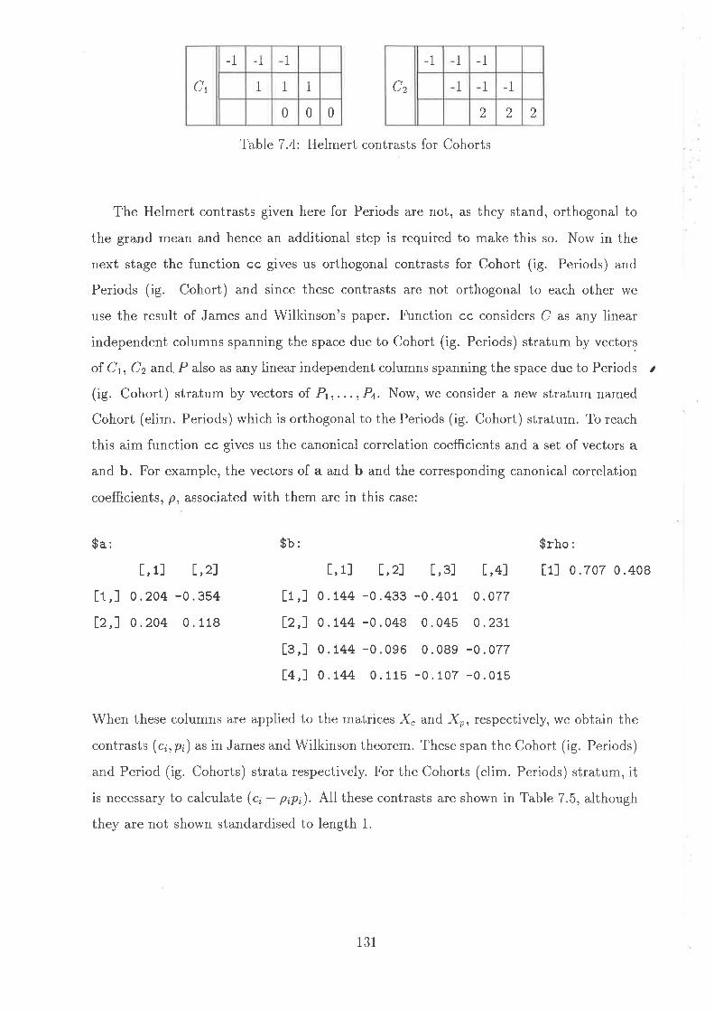
Ct
-1 -1 1
1 1 1
0 0 0
Cz
1 I -1
1 1 -1
2 2 2
Table 7.4: Helmert contrasts for Cohorts
The Helmert contrasts given here for Periods are not, as they stand, orthogonal to
the grand mean and hence an additional step is required to make this so. Norv in the
next stage the function cc gives us orthogonal contrasts for Cohort (ig. Periods) and
Periods (ig. Cohort) and since these contrasts are not orthogonal to each other we
use the result of James and Wilkinson's paper. Function cc considers C as any linear
independent columns spanning the space due to Cohort (ig. Periods) stratum by vectors
of C1,, Cz and.P also as any linear independent columns spanning the space due to Periods ,(ig. Cohort) stratum by vectors of Pyr. . . , P¿. Now, we consider a new stratum named
Cohort (elim. Periods) which is orthogonal to the Periods (ig. Cohort) stratum. To reach
this aim function cc gives us the canonical correlation coefficients and a set of vectors a
and b. For example, the vectors of a and b and the corresponding canonical correlation
coefficients, p, associated with them are in this case:
$a:
[, 1] l,2f
[t,] o .204 -0.354
lz,f 0.204 0.118
$¡:
[, t] l,z) [,3] [,+]
[t,] 0.r44 -0.433 -0.401 o.o7T
12,f 0 .744 -0.048 0.045 0.231
[9,] o .r44 -0.096 0.089 -o .orT
[+,] 0.144 o.11s -0.107 -o. o1s
$rho:
t1l 0.707 0.408
When these columns are applied to the matrices X" and Xo, respectively, we obtain the
contrasts (.o,p) as in James and Wilkinson theorem. These span the Cohort (ig. Periods)
and Period (ig. Cohorts) strata respectively. For the Cohorts (elim. Periods) stratum, it
is necessary to calculate (c¿ - p;p¿). All these contrasts are shown in Table 7.5, although
they are not shown standardised to length 1.
131

c p t - p? Cohort(ig. Periods) Periods(ig. Cohort) Cohorts (elim. Periods)
3 3 rl21
0
1
I
0
1
-10
1
-2-1
0
1
0
1
0
1
2
0
1
2
1
0
1
2
1
0
516
1
2
1
1
2
1
1
2
1
2
1
0
I
0
1
0
1
2
03-3 -423
2
-t)
0
4
-51
5
1
4
1
4
-5
-2-1
tt
1
3
2
,l
2
1
Table 7.5: Contrasts for three cohorts and three periods
For convenience, we write the CohortxPeriods aiiay as a rectangle in which cohorts are
represented by rows and successive periods are represented by successive reverse diagonals
of the aray; that is, the sets of value running along diagonals from top right to bottom
left. It can then be seen that the period contrasts are in fact contrasts between periods,
while the Cohort (elim. Periods) contrasts are orthogonal to periods.
7.7 .I Projector matrices
For this design we have
r ,9s : Ils I ../s for Cohort (ig. Periods)
r ^91 : Ð|=tp¿p'¿ for Periods (ig. Cohort)
o 52 : D?=t +(ci - p¿)(ci - p¿p¿)' for Cohort (elim. Periods)
r ,93 : (Is A 1r) - (J,6 "f.) - (S, 1Sr) for PeriodxCohort interaction,
where it is assumed that both q and p¿ are standardized to length 1.
t32

7.8 To get a pattern on p and the Cohort (elirn. Pe-
riods) contrasts
To get a pattern on p and the contrasts for the Cohort (elim. Periods) stratum lve have
written the results in Table 7.6 for c -- 2 and Table 7.7 for c : 3. For c : 2, there is one
contrast for Cohorts (elim. Periods), and it is obtained by deleting the values in the first
and last periods and taking the average difference between the other means. This has
(1- p'): (p-l)f p, so that the expected mean squa e for this contrast is o2 +(p- l)"?,
plus lvhatever treatment terms it estimates
c p t-p? Cohort(elim. Periods)
2 2 0.5000 1
1 0
2 3 0.6670 -1 1
1 1 0
2 4 0.7500 -1 1 1
1 1 1 0
2 5 0.8000 1 -1 1 1
1 I 1 1 0
Table 7.6: Canonical correlation coefficients and orthogonal contrasts for two cohorts and
various periods
When c : 3, there are two such contrasts, with (t - p?) equal to 1 - 3l(2p) and
t - t lQe). The two contrasts have a consistent pattern, representing, respectively, a
linear and quadratic contrast of the cohorts through the middle p - 2 periods, withslight adjustments at the ends, and having expected mean squares of o2 + (p - t)o! and
o' + (p - I)"?, respectively.
2 6 0.8330 -1 -1 1 1 1
1 1 1 I 1 0
2 7 0.8570 1 1 1 -1 1 -1
I 1 1 1 1 1 0
2 8 0.8750 1 -1 -1 1 1 -1 -1
1 1 1 1 1 1 1 0
133
0 -1 0 1
1 1 i 13 2 0.250 0.750
1 0 I 0
0 -1 o 0 ó 2
1 0 -1 Ð -4 -33 3 0.500 0.833
2 1 0 2 3 0
0 -1 2 2 0qd 2 2
1 0 0 1 -.) -4 -4 -ó3 4 0.625 0.875
2 2 I 0 2 2 3 0
0 1 , Ð Ð 0 ð 2 2 2
1 0 0 0 I -.) -4 -4 -4 -ù3 5 0.700 0.900
2 2 2 I 0 2 2 , .) 0
0 3 2 2 2 2
-3 -4 -4 -4 -4 -3
0 2 2 -2
0 0 0
2 2 2
-1
1 1
1
3 6 0.750 0.917
Ð
2
0
2 2 2 2 e) 0
2
-4 3
0 2 .)0 3 2 2 2 2
0 0 1 3 -4 -4 -4 -4
2 2 1 0 2 2 2 .)
1
I
-2 -2 -2
3 7 0.786 0.929 0
2
0
2
0
2 2 3 0
cp r- p? t- p3 Cohort(elim. Periods) Cohort(elim. Periods)
Table 7.7: Canonical correlation coefficients and orthogonal contrasts for three cohorts
and various periods
7.9 Conclusions
The above analysis provides a set of contrasts among the Cohorts, orthogonal to Periods,
which will enable estimation of treatment effects. Each contrast will have a different
expected mean square, so that the treatment information from each normalised contrast
will need to be combined with a different weight. Furthermore treatment information
will be available in the CohortxPeriod interaction, and each normalised contrast in that
space will have variance o2. In the next chapter, we consider some particular designs and
demonstrate how much information is available and how it can be recovered.
134

Chapter 8
Treatment structure of cohort
designs
8.1 Introduction
Having examined the block structure of cohort designs in the previous chapter, we now
turn our attention to treatment structure. We consider the specification of linear treat-
ment models when treatments are applied to the experimental subjects, and we get
formulae for the analysis of cohort designs which have a linear treatment model and a
non-orthogonal block structure. To extend our approach to analyse crossover trials effi-
ciently as we did in Chapter 6, we apply the cohort design methodology to a number of
different crossover trials . In Section 8.2, we describe how to obtain treatment estimates
from cohort designs, and in Section 8.3 we extend the results of Chapter 7 to the case
where there are g groups of subjects in each of the cohorts, the idea being that each group
within a cohort is given a different treatment regime. Subsequent sections then consider
a number of possible designs and compare the results with those obtained earlier in this
thesis for the corresponding standard design.
135
8.2 Treatment structure for cohort and standard de-
signs in general
To shorv the efficiency of the cohort design and the results of James and Wilkinson's
theorem in a nonorthogonal block structure, we estimate the treatment effects in a cohort
design and then compa e it to a corresponding standard design. To refer to previous
chapter we now consider the general cohort and standard designs with length cpgn, for
both designs, where there are c cohorts, g groups within each cohort, and each of the rz
subjects rvithin each (cohort, group) combination is observed for p periods. Since the rz
subjects within a group all receive the same treatment regime, we can consider just the
vector of length cpg which consists of the group means at each time. In terms of seeing
where treatment information resides, we can without further loss of generality consider
the case where n -- l.
We assume that the design has s treatment parameters and the linear model for
treatment and grand mean for both designs is expressed in Chapter 6 in equation (6.3.1).I l/
Suppose ds - | U 0' I represents the parameters other than the group and period
parameters, and suppose that the vector of treatment effects d has s elements. Let
?s represent the corresponding design matrix and suppose that its (s * 1) columns are
linearly independent.
The vector á might include ro¡ rD, )6, and À¿, which we introduced in Chapter 6.
However, we want to consider at this stage a general set of treatments which might
even include factorial contrasts, for example. To consider what treatment information
is available, we take the matrix ?6 for treatments in a model with length cpg. Then
the information matrix overall it \fo when the grand mean is considered. Sone of the
columns of 7s corresponding to particular parameters may be orthogonal to the 1 vector.
Since the estimate of the grand mean p does not provide any useful information about
treatments, the only usable information is contained in the bottom right-hand s x s
submatrix of f[Q - J)To. If we let f. : I L fö ], u.r'a define
T : (r _ J)T;,
then the required information matrix for 0 is TtT.
If we split the observation vector into several strata, using orthogonal idempotent
136

matrices Qo., Qr, . . .Q x where D!:o Q n: 1, then we can rvrite
u:(Qo-fQtI...+Q¡)v,
where Qog.,QtU,. ..Qny are components of the variation among different strata, and the
treatment information for the ith stratum isT'Q¿T.In the case where Var(e) - o2I,
0: çT'T¡-|T'y,
but if each stratum has variance matrix 6¿Q¿ then the combined estimate is
k
B : {D 6¿rT,giT}-lt 6ntT,gny
andk
V ar(O) : iD 6;LT' q¿Tj-r,
where, as in previous chapters, the summation is made over those values of i for which
we believe we have useful information. As before, we would exclude components such as
the grand mean (i : 0), and strata involving period efiects since they can not generally
be well estimated or a variance coÍrponent determined. In the case of a cohort design,
we would generally not try to use information from Period(ig Cohort) stratum, but the
information from the Cohorts(elim. Period) stratum would be used.
8.3 Projector matrices for cohort and standard de-
signs in general
We know that the projector matrices for the standard design, in the case ?? : 1, are as
shown in Table 8.1.
And for the cohort design we have the projector matrices shown in Table 8.2 where
S¿ are cp x cp matrices defined in the previous chapter.
t37

Stratum Projector matrices for Standard Design
Periods J"Øl(eØJs
Cohorts
Groups within Cohort I"Ø Jp Ø I(s
Period x Cohort I{"ØI(eØJs
Periods x (Groups within Cohort) I"Ø KpØ I{s
Table 8.1: Projector matrices for general standard design
Stratum Projector matrices for Cohort Design
Periods (ig. Cohorts) SrØJs
Cohorts (elim. Periods) SzØJs
Groups within Cohort I"Ø JpØ Ks
Periods x Cohort SsØJs
Periods x (Groups within Cohorts) I"Ø Ke Ø I{s
Table 8.2: Projector matrices for general cohort design
\Me note that in Cohort (elim. Periods) in the general case the information is contained
in (c - 1) separate l-dimensional subspaces and is given by
T'(CuØ Js)T (i:1,...,c- 1)
where C¿ can be interpreted as d¿d'¿ such that d,¿ is a contrast of length 1. Then the
projector matrix for d¿ is
d' ¿(d''¿d'¿)- |
d,'¿ : d¿ d¿,
where
d,i: -+k¿ - p¿p¿),
lr-Piand c¿,p¿ and pi are as defined in Chapter 7.
T'(Co Ø Js)T T'(didi Ø Js)T
!T'@,0d,',8 1r.')?gI
ir'@,8 1)(d; I 1)'7
(8.3.1)
1
?,'g-uiw
138

It follorvs that the information in the ith l-dimensional subspace of Cohort (elim. Periods)
is given by jw;wi, rvhere LD¿: T'(d¿Ø 1). Correspondingly, the projector matrix for
Periods (ig. Cohorts) stratum i. Ðf]'-'p¿pt¿, and since the length of p¡'s are I then the
information matrix for this stratum can be lvritten as
P*c-2T'{5, Ø Js}T : r'{ Ð P¿P'¿ Ø Jn}T (8.3.2)
z'{ Ð (ro ø t;1oo 81)'}"1
g
1
i=1p*c-2
i=lP*c-2
D q¿q'¿,
i=lg
where q,i : Tt(pi Ø I).
If we have n ) 1. subjects in each group, then the ANOVA's will have two more lines,
corresponding to Subjects within Groups and Periodsx(Subjects within Groups) strata.
As before, these will contain no treatment information, and will provide estimates of o2
and o2 + paz, respectively.
8.3.1 Estimates of parameters and covariance matrix of esti-
mates
To get the estimates of parameters we combine the estimates of parameters from those
strata in which there are some information about parameters. Thus we can write
â : {:r l;''(c¡ I ")')- å [ä''(8' ø
")"]] (8 3 3)
{= [;' ,(c¡ Ør,r] * Ð-lir,,o,*
r")] ],,
and covariance matix of d is
var(g): {Ë lï,''"'s /,)r] - å i;t '(Q¿ Ø",t]} (8 3 4)
where \j : o2 + p"?(l - p3) (j : 1,2,...,"- 1) and ds - du : o2 and 6s: o2 + po?.
In the rest of this chapter we examine the result of James and Wilkinson theorem in
some special cases of standard and cohort designs.
139

8.4 Treatrnent inforrnation for two-treatrnent crossover
design with two baseline measurements and a
corresponding cohort design
We nolv examine the treatment information for the two-treatment, crossover with two
baseline measurements, one before the first treatment period and one after this period.
As Kenward & Jones (1987b) concluded, one reason to use two baseline measurements in
the 2 x 2 crossover designs is to increase the power of test for the presence of carryover
effects by splitting the sum of squares between-subjects into various components which
can be used to analyse these designs. Freeman (1989) gives us another reason to take the
baseline measurements in the 2 x 2 crossover design. He and others have suggested that
use of baseline measurements, leads to a unique resolution of the estimation difficulties
which we face in the simple crossover designs. In this section, we consider the consequence
of the use of baseline measurements and in the next subsection we look at what happens
if we withdraw the canyover effect in this design. These extra periods give the design
which is shown in Table 8.3.
Period
1 2 ù 4
Group 1
2
A B
B A
Table 8.3: Two-treatment crossover design with two baseline measurements
Now in this study we consider a cohort design with c : 2., p: 4 and g : 2 but n : 1,
then the layout of design is shown in Table 8.4 with a delayed entry at period 2 for
the second cohort. Subjects within a cohort would be randomly allocated in equal-sized
groups to the treatment regimes.
140

Period
1 2 ù 4 5
I
2
3
4
Group
A B
B A
A B
B A
Table 8.4: Cohort design in two-treatment, two-period crossover design with tlvo baseline
measurements.
By referring to Table 8.4, we first write out the 16 expected values in the following
table which could be applied to either the standard or the cohort design. Using the
notation of Chapter 5, the expected values in each cell are as shown in Table 8.5.
ll IL+ro+rD ¡;*Ào*)o p,lro-rnp p,*rro-ro p'*Ào-Ào p,+ro+rD
p p+ro+rD ¡r*Ào*)p p'Iro-rop p'lro-rn p*)o-)o p,+ro+rD
Table 8.5: Expected values of two-treatment, two-period crossover with two baseline
measurements when we consider the cohort design or double standard design.
Our purpose in the two following subsections is to get the treatment information for
this case. We now first consider the model which includes the first-order carryover effect
and in the next subsection we analysis the model without the first-order carryover effect.
t4r
8.4.L Treatment information when the first-order carryover is
present
If lve 1et y be a vector of observations corresponding to the 16 expected values written in
order across the rows, then by referring to the linear model expressed in 8.5 we have
To: Iz Ø
T,T :
00 0
00 0
10 1
10-101 0
01 0
10-110 1
1 0
0
0
0
1
1
0
0
1
1
1
1
1
1
-4-4
4
4
-4-4
4
4
-2-2-2
q
6
6
-2-2
1
where 12 arises from the fact that there are two cohorts, both using the same treatment
structure and ds : þ, Tot )0, TD¡ Àn . The matrix ?, obtained by eliminating
the effect of the 1 vector from the columns of 7s is then given by
T:!1,ø8'-
0
0
8
8
0
0
8
8
0
0
0
0
8
8
0
0
(8.4.1)
so that the overall treatment information is
4
-20
0
00008004
2
.)
0
0
Table 8.6 shows the information matrices for the different strata in each design obtained
by calculating T|Q¿T for the appropriate idempotent matrices Q¡. In the case of the
standard design, we use the Kronecker product matrices sholvn in Table 8.1. For the
r42
cohort design, we refer to Table 7.6 in the previous chapter, lvhich shows that lvhen c:2and p : 4, we have one degree of freedom for Cohort (elim. Periods) with p1 : 0.50, and
d1 given by the contrast in Table 8.7.
Table 8.6: Information matrices for standard and cohort designs in two-treatment design
lvith two baseline measurements, when first-order canyover effect is present
Stratum
Standard Design Cohort Design
o2 o2" Information Matrix p 02 o 2 Information Matrixt
Periods(ig. Cohorts)
4
-20
0
2
3
0
0
0
0
0
0
0
0
0
0
1
0
0
0
000i00000000
Cohorts(elim. Periods) t4 None
1
0
0
0
000
1
3
0000.50 1 3
000000
Group within Cohorts I4
0000000000000001
t4
0000000000000001
Periodsx Cohorts 10 None 10 n
3
4
-30
0
-300300000000
Periods x (Grp.w.Coh.) 10
0000000000800003
10
0000000000800003
4
2
0
0
2
3
0
0
0
0
8
0
0
0
0
4
4
-20
0
2
3
0
0
0
0
8
0
0
0Total
0
4
t43

0 -1 1 1
0 -1 1 -1
1 1 1 0
I i 1 0
Table 8.7: Orthogonal contrast on Cohort (elim. Periods)
In comparing the results in Table 8.6, in terms of treatment information in each design
and in each stratum,, the follolving points can be noted:
o The treatment information in Group within Cohorts and Periods x (Grp.w.Coh.)
strata for both designs is the same, because the projector matrix in each stratum
is the same for both designs.
o In the standard design, all information about (ro, )o) is in the Periods stratum,, so
that the possible presence of period effects would imply that we cannot estimate
(ro, )o) 'vith this design.
¡ In the cohort design, most of the information about (ro, Ào) is available in Period x Cohort
stratum with a variance of ø2 and some information (11%) about 16 is in the Cohorts
(elim. Periods) stratum with a variance of o2 +3o?.
8.4.2 Tleatment information when carryover efÏect is not present
Now we consider this crossover design when there is no carryover effect in the model.
We refer to Table 8.5 and do not consider the two parameter Ào and )¡. Then the total
treatment information for direct treatment only can be written as
4008
The treatment information in five different strata for direct treatment effect for standard
and the cohort designs is given in Table 8.8.
T,T
t44

Standard Design
Stratum o2 o! Information Matrix
Periods(ig. Cohorts)0 0
40 1000
Cohorts(elim. Periods) NoneI4
Group within Cohorts Nonet4
Periods x Cohorts None10 1
310
0 0
80
Periods x(Grp.w. Coh.) 10 0008
10 0008
Total4008
4008
Cohort I)esign
p o2 o! Information Matrix
0.50 1 3 -L3
0
0
1
0
T4 None
Table 8.8: Information matrices for two-treatment, two-period standard and cohort de-
signs when first-order carryover effect is not present.
Like the situation in the previous subsection with this same design but with first-order
carryover effect,, cohort design is more efficient than the standard design. The parameter
re is estimable in all strata except the Groups within Cohort stratum and for rp ,the
difference between direct treatments, Periodsx (Groups within Cohorts) in both designs
has all the information.
8.5 TYeatment information for two-treatment, extra-
period crossover design and its corresponding co-
hort design with one baseline measurement
In this section we consider the extra-period crossover design with two treatments and
one extra period for baseline measurement. This design with three treatment periods
with two groups is known as a dual balanced design, because this design is made up
of equally replicated pairs of dual groups. The reason to choose this design is that the
additional treatment period decreases many of the problems associated with analysis of
t45
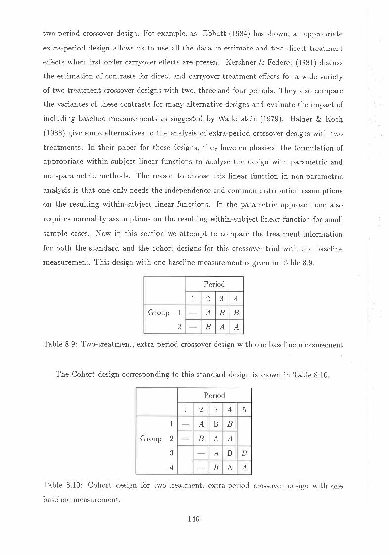
trvo-period crossover design. For example, as Ebbutt (1984) has shorvn, an appropriate
extra-period design allolvs us to use all the data to estimate and test direct treatment
effects u'hen first order ca ryover effects are present. I(ershner & Federer (1981) discuss
the estimation of contrasts for direct and carryover treatment effects for a wide variety
of two-treatment crossover designs lvith two, three and four periods. They also compare
the variances of these contrasts for many alternative designs and evaluate the impact of
including baseline measurements as suggested by Wallenstein (1979). Hafner & Kocþ
(1988) give some alternatives to the analysis of extra-period crossover designs with two
treatments. In their paper for these designs, they have emphasised the formulation of
appropriate within-subject linear functions to analyse the design with pararnetric and
non-parametric methods. The reason to choose this linear function in non-parametric
analysis is that one only needs the independence and common distribution assumptions
on the resulting within-subject linear functions. In the parametric approach one also
requires normality assumptions on the resulting within-subject linear function for small
sample cases. Now in this section we attempt to compare the treatment information
for both the standard and the cohort designs for this crossover trial with one baseline
measurement. This design with one baseline measurement is given in Table 8.9.
Period
1 2 3 4
Group 1
2
A B B
B A A
Tabie 8.9: Two-treatment, extra-period crossover design with one baseline measurement
The Cohort design corresponding to this standard design is shown in T.Lle 8.10
Table 8.10: Cohort design for two-treatment,, extra-period crossover design with one
baseline measurement.
Period
1 2 3 4 5
I
2
o,)
4
Group
A B B
B A A
A B B
B A A
t46

The expected values of the design for this model are given in Table 8.11
I,r lr+ro+rD þiro*)o-rolÀn p,lro*Ào-ro-Àop p.*ro-rn p'lro*)o*rn-Ào þlro*)o*ro*Àop lt+ro+rD L¿*ro*)o-rnI\n ¡.r,I ro * )o - ro - Àn
ll p,*ro-r¡t p,*ro*)o*rn-Àn ¡t"Iro*)o*rnIÀnTable 8.11: Expected values for design of two-treatment, extra-period crossover trial
Now, as in the previous section, we deal with this design in two subsections in terms
of presence and absence of first-order ca ryover effect in the model.
8.5.1 Tleatment information when first-order carryover effect
is present
The total treatment information for both the standard and the cohort designs after taking
o':t the vector 1 due to the grand mean can be obtained as
7"7 :
The output from SPLUS and Maple software provides the information matrices for var-
ious strata for both designs as given in Table 8.12. Treatment information about the
differences rp and )¡r remain the same for the two designs, with a small amount of in-
formation in the Groups within Cohorts stratum. The situation, however, is different fro
the treatment information which looks at how the average of the two treatments differs
from baseline. In the standard design, this is totally lost to the Period stratum. For the
cohort design, not much is recovered, with only a third of the information about r¡ and
a quarter of the information about Às being recovered, the rest being lost into the Period
stratum.
The Cohort(elim. Periods) stratum has the information about (ro, )o), and this is
contained in the one degree of freedom contrast
32 0 0
24 000012000 08
747

0 -1 1 -1
0 -1 1 1
I 1 I 0
1 1 1 0
which in this case has expectation
2(2rç ! )o) - 2(3ro -l2)o) : -2(ro * Ào),
and variancel2(o2 +3o!). The PeriodxCohort stratum has just 2 degrees of freedom
These may be represented by
which have expectations of 2(D,s - rs) and -2ro, and variances of 24o2 arrd 8a2,, respec-
tively. It follows that the information matrix for these two contrasts is given by
1
3
r12 ]+ z
1
6
1 2 1
1 l;lr -1 02
as given in Table 8.12.
l2
0 1 2 -l0 1 2 -1
I -2 1 0
1 -2 1 0
0 I 0 1
0 1 0 I
1 0 -1 0
1 0 1 0
r48

Stratum
Standard Design Cohort Design
o2 o , Information Matrix,9
p 02 o! Information Matrix
Periods(ig. Cohorts)
32 0 0
240000000000
220023 0 0
00000000
Cohorts(elim. Periods) t4 None
1
1
0
0
100
11000.50 1 3
000000
Group within Cohorts 74
0000000000100000
74
0000000000100000
Periodsx Cohorts 10 None 10 I
2
-10
0
-1 0 0
200000û00
Periods x (Grp.w. Coh.) 10
00 0000 000 0 11 0
00 08
10
00 0000 000 0 11 0
0 0 0832 00
Total2
0
0
4
0
0
0012008
3 2
4
0
0
0
0
0
0
0
8
2
0 t2
0 0
Table 8.12: Information matrices for standard and cohort two-treatment, extra-period
designs with one baseline measurement.
This information can ed to form treatment estimates by rveighting these
contrasts by their inform ces, i.e.
l;l : {;ll rl ', ;l}
r49

x {lll lll;: l.+'l ; ;ll;; l.='l; :ll;. 1}in which îot, îoz, âe3 represent estimates obtained from the three contrasts, one from
Cohorts(elim. Periods) and the other two from PeriodsxCohorts. Now lve can write
-1t6pTg
io ['
{t
3p
-ôp3*6p
1
1
X (î0, * io,) * 1*3p2
0 rrp 0 -p0 l*p 0 -p
_1r + n) 0 p 0
_1r + n) 0 p 0
0 0 1r+n) -p0 0 1r+n) -p
0 _1r + r) p 0
0 _1r + r) p 0
I ;l(î"-zi") +le+iø l;l-')
i;l
r [r+p p .l
3(r+pxl +spL p ,*rr)
{ll](î.'*i.') -F'j# t ;] (î.,-z\.,)+
: --+;l{III(îor*io') +tl-,1 ,, I(ìo'-2io')
+;[';"]"Then the estimate of rs can be obtained as the following linear combination of the 16
treatment means:
X3(1 + 3p)
los2
I,o - z(r+p)
and the estimate of )s is similarly given by
\-1no - zÍ+p)
The variance of these estimates is given by
Tg | -l2p
p
p
1*2p)oVar
150

\A,¡e note again that this refers to the case n - 1 subject in each group in each cohort,
and an increase in the value of n lvould simply reduce this variance by a factor of n.
8.5.2 Treatment information when the first-order ca.rryover is
not present
We here again consider the design in the previous subsection, but we discarcl the first-
order carryover effect from the model. Just for the direct treatment effect rve have the
total treatment information
,'r:u 300 ).2
and subsequently the treatment information separately for various strata is ol¡tained for
both standard and the cohort designs as in Table 8.13.
Cohort Design
p 02 o! Information Matrix
2000
2
0
010 !3
0
Table 8.13: Treatment information for both standard and cohort two-treatment, extra-
period design with one baseline when the carryover effect is not present.
Standard Design
o! Information Matrixo2Stratum
3000
Periods(ig. Cohorts)
Nonet4 0.50 I 31
3
1000
Cohorts(elim. Periods)
lolo
0
1
14 I 40001
Group within Cohorts
None10Periods x Cohorts
0
11
0
010 0
11
0
0Periods x(Grp.w. Coh.) 1 0
0
12
r)
0
0
72
ot)
0Total
151
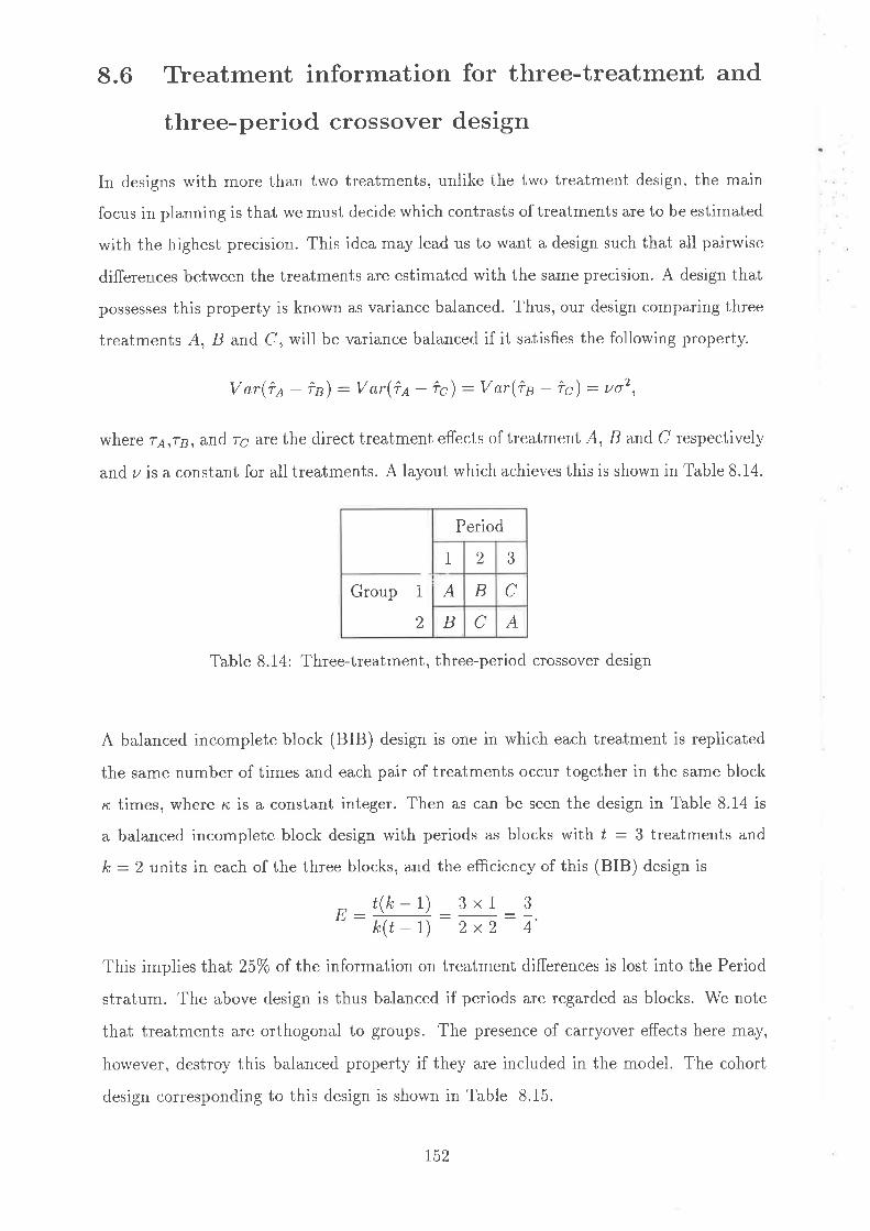
8.6 Treatment information for three-treatment and
three-period crossover design
In designs with more than two treatments, unlike the two treatment design. the main
focus in planning is that we must decide which contrasts of treatments are to be estimated
with the irìghest precision. This idea may lead us to want a design such that all pairwise
differences between the treatments are estimated with the same precision. A design that
possesses this property is known as variance balanced. Thus, our design comparing three
treatments A, B and C, lvill be variance balanced if it satisfies the following property.
V ar(î¿ - îa) : Var(ît - îc) : V ar(î'p - îc) : Lto2,
where rA,,rB, and r¿ are the direct treatment effects of treatment A, B and C respectively
and u is a constant for all treatments. A layout which achieves this is shown in Table 8.14.
Group 1
2
Period
1 2 3
A B C
B C A
Table 8.14: Three-treatment, three-period crossover design
A balanced incomplete block (BIB) design is one in which each treatment is replicated
the same number of times and each pair of treatments occur together in the same block
rc times, where rc is a constant integer. Then as can be seen the design in Table 8.14 is
a balanced incomplete block design with periods as blocks with ú : 3 treatments and
k : 2 units in each of the three blocks, and the efficiency of this (BIB) design is
n ¿(k-1) 3x1 3"-k(t-1)-zx2-4'
This implies that 25% ol the information on treatment differences is lost into the Period
stratum. The above design is thus balanced if periods are regarded as blocks. We note
that treatments are orthogonal to groups. The presence of carryover effects here may,
horvever, destroy this balanced property if they are included in the model. The cohort
design corresponding to this design is shorvn in Table 8.15.
752
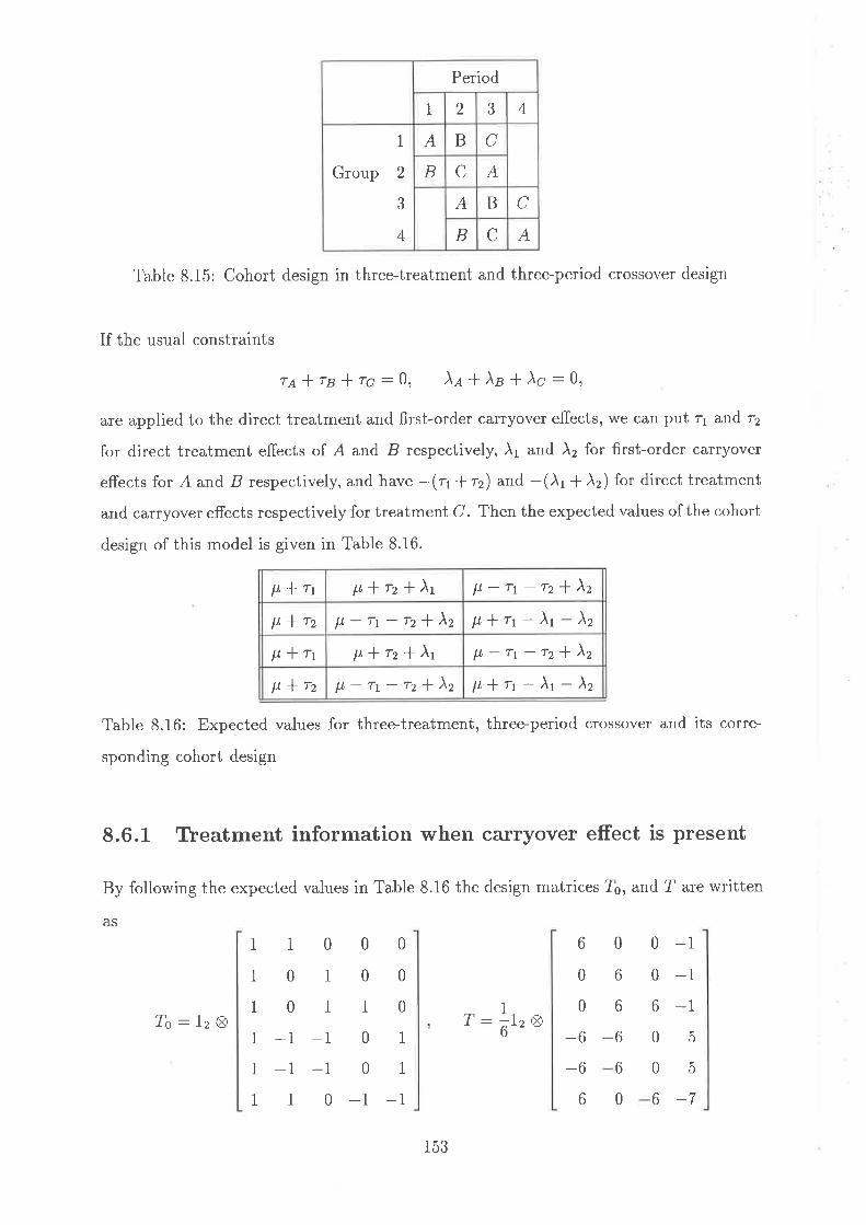
Period
1 2 ô 4
I
2
.)
4
Group
A B C
B C A
A B C
B C A
Table 8.15: Cohort design in three-treatment and three-period crossover design
If the usual constraints
r¡*rn*rc:0, À¿ *À¡ *)c:0,
are applied to the direct treatment and first-order carryover effects, r¡/e can put 1 and 12
for direct treatment effects of A and B respectively, )1 and À2 for first-order carryover
effects for A and B respectively, and have -(1 f 12) and -()r * À2) for direct treatment
and carryover effects respectively for treatment C. Then the expected values of the cohort
design of this model is given in Table 8.16.
p,*rr p,l rz I Àt H-rt-rzlÀzp'Irz F-rt-rzlÀz p,+ rt-Àr-)zp,lrr p,*rzl\r þ-rt-rz*Àz
¡L' I rz þ-\-rzl\z p,*rr-)r-)z
Table 8.16: Expected values for three-treatment, three-period crossover and its corre-
sponding cohort design
8.6.1 Treatment information when carryover effect is present
By following the expected values in Table 8.16 the design matrices ?s, and T are written
AS
1110101 -11 -111
0-10-16-105056-7
000100110
-1 0 1
-1 0 1
0-1-1
6
0
0
-6-6
6
0
f)
6
6
6
0
Zo:128
153
T: !1, m6--
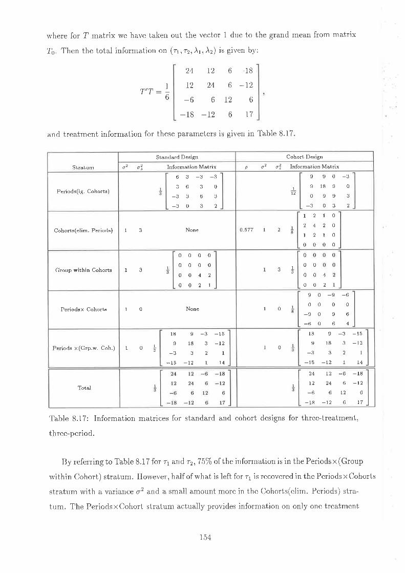
where for T matrix we have taken out the vector 1 due to the grand mean from matrix
To. Then the total information on (21 ,r2,,Àt,)2) is gìven by:
T,T
and treatment information for these parameters is given in Table 8.17
Table 8.17: Information matrices for standard and cohort designs for three-treatment,
three-period.
By referring to Table 8.17 for ?'1 and 12,75% of the information is in the Periods x (Group
within Cohort) stratum. However, half of what is left for 11 is recovered in the Periods x Cohorts
stratum lvith a variance o2 and a small amount more in the Cohorts(elim. Periods) stra-
tum. The Periods x Cohort stratum actually provides information on only one treatment
I:-6
24
I2
-6-18
12
24
6
-12
-66
12
rt
-18
-t26
T7
Stratum
Standard Design Cohort Design
o2 o2, fnformation Matrix p o' ot" Information Matrix
Periods(ig. Cohorts)
6336ÐÐ
-30
-33
6
0
,
1
12
9
9
0
Il8
Io
0-39093
Cohorts(elim. Periods) 13 None
1
t
Io
|,1 0
0
0
0
4 t0.577 I 2
21o0
Group within Cohorts 13
0
0
0
0
0
0
0
0
0
0
4
2
0
0
1
I 3 1
0
0
0
0
0
0
0
4
Periodsx Cohorts lo None I 0
90oo
-90-60
-9 -6o09664
Periods x(Grp.w. Coh.) 1 0 I
18
I
-3-15
I18
-t2
-3
2
1
-15-12
1
l4
1 0
18
I
-3-15
9
18
-t2
-33
J
1
-15
-121
l4
Total
24
I2
-6-18
L2
24
6
-72
-66
t2
6
-18-12
6
l7
754

combination, namely 3rr - 3)r - 2À2, rvhile Cohorts(elim. Periods) has information only
on the linear combination rr * 2^2 + ^1.
8.6.2 Tleatment information when carryover effect is not present
The total information for just direct treatment effect after taking out the grand mean
from the matrix design of the model is
T'T : l;:land treatment information for both standard and cohort design is given in Table 8.18.
It shows that, of the25% of the information lost to Periods in the standard design, about
half of this is recovered for 11 from the Periods x Cohorts stratum,, and a quarter of it
for 12 is recovered from the Cohorts(elim. Periods) stratum. It may be possible to do
better than this by astute choice of design or by extending the design to three cohorts.
Cohort Design
p o2 o! Information Matrir
13 None
Table 8.18: Treatment information for both standard and the cohort designs in three-
treatment, three-period when the carryover effect is not present.
Standard Design
Stratum Information Matrix2 ,o o I
Periods(ig. Cohorts)2l12 Z
1
2
1
1
None13Cohorts(elim. Periods) 0,577 1 2 1
8
t224
None13Group within Cohorts
Periods x Cohorts None10 I8
10 9000
Periods x(Grp.w. Coh.) où10 27
t2I 0 ,l
2l72
Total 42TI2
4I 2
2t
155

8.7 TYeatment information for two-treatment with
one baseline measurement with more than two
cohorts
In Chapter 6 we analysed this design with two cohorts, now we see what happens when
we analyse with more than two cohorts. The layout for this case is shown in Table 8.19.
Table 8.19: Two-treatment crossover design with one baseline measurement when c : 3
The means corresponding to these 18 groups can be written as in Table 8.20
ll p,lro*rn p,lro*)o-rplÀop p'lro-ro p,*ro*Ào*rn-Ào
ll y,+'ro*ro p,*ro*Ào-ro*Àop p,lro-ro p,*ro*)o*rn-Ànp p,*roIro p,*ro*Ào-rnlÀop p,lro-ro p,lro*)o*rn-Ào
Table 8.20: The 18 means for two-treatment with one baseline measurement lvhen c: 3
As for the previous designs, we consider this case in two stages, with and without first-
order carryover effect.
Period
1 2 3 4 5
1
2
or)
4
b
6
Group
A B
B A
A B
B A
A B
B A
156

8.7.1 Tleatment information when c - 3 and first-order carry-
over effect is present
By referring to Chapter 7 and considering the means repeated three times due to c : 3,
and also the different ordering to put the design matrix, then the design matrix Ts can
be presented as belolv
?o:ls8
00 0 0
00 0 0
10 1 0
10-1 0
I 1 -1 1
1 1 1 -1
r:fr,ø
0
0
0
0
6
6
1
1
1
1
I
1
-4-4
2
2
2
2
2
2
2
2
4
4
0
0
6
6
6
6
and the total information for this case is
T,T
42 0
24 0
00 t2
00-6
0
0
6
6
This information is now partitioned among the different strata as shown in Table 8.21.
We see that, in the cohort design, about 60% of the information about ro and Ào is
recovered in the various strata, with some appearing in the Cohorts (elim. Periods) and
some in the Cohort x Period interaction.
r57
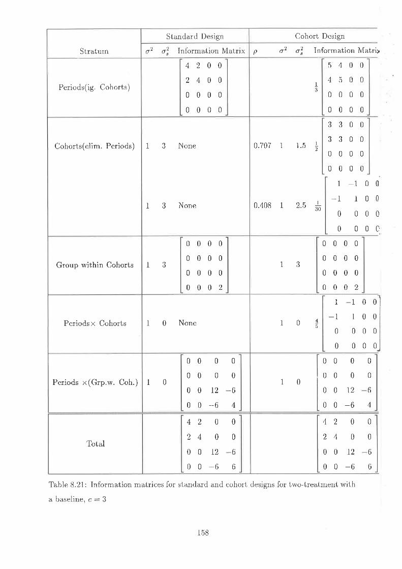
Standard Design
Stratum Information IVIatrix2o o2
4200240000000000
Periods(ig. Cohorts)
Cohorts(elim. Periods) 1 3 None
1 3 None
Group within Cohorts
0000000000000 0 02
13
1 0 NonePeriods x Cohorts
0
0
0
0
00000 1.2
0-6
0
0
6
4
10Periods x(Grp.w. Coh.)
Total
42 0
24 0
001200-6
0
0
6
6
Cohort Design
p o2 o! Information Matri>
0.707 1 1.5 I2
0.408 | 2.5 #
540045 0 0
0000000033.) .)
0000
I
-10
0
00000000-1
1
0
0
I
0
0
0
c
0
0
0
0
13
10î
10
0000000000000 0 02
1-1 00-1 1 0 0
0 0000 000
00 0
00 0
00 t2
00-642 0
24 0
001200-6
0
0
6
4
0
0
6
6
Table 8.21: Information matrices for standard and cohort designs for two-treatment with
abaselinerc:3
158

8.8 Concluslon
As we showed, classical analysis of crossover design even if baseline measurements are
included and in the presence of strong or unknown period effects is unable to recover
information about the difference between the average treatment effect and baseline. Using
the cohort design in crossover design, we can recover some information about (16, )s) and
obtain estimates for them from within and between subjects. This method opens the
way for a more detailed examination of the topic and in this chapter lve have examined
various crossover designs.
In comparing the cohort and standard designs and to show the abilities of cohort
designs to recover some information about the parameters of interest, consider the infor-
mation matrices in Table 8.22 in three cohort designs in the analysis of two-treatment,
two-period crossover design with 1,, 2 and 3 cohorts, or equivalently, c : l, c: 2 and
c: 3 respectively. We note that c : I is equivalent to the standard design.
Information matrix
Strata C:I C:2 C:3
Periods(ig. Cohorts) I6
8448
1
6
108810
1
6
10 8l810
I
Cohort(elim. Periods) ,l: :l *lII ;l
ål0.2
-0.2
-0.2
0.2
Periods x Cohorts 1tt
3-3
-3316
4.8
-4.8
-4.84.8
Total !b
8448
1
6
168816
I6
24 t212 24
Table 8.22: Information on rs and Às in three cases of design
As can be seen,, the total information will increase when we increase the number of
cohorts in the model. In addition in the standard design (c : 1), all information about
the parameters of interest is in the Periods(ig. Cohorts) stratum, although in the cohort
designs (c : 2,3) the information is distributed in all strata, and the proportion of the
159

information recoverable increases, being close to 40% lvhen c:2 and nearly 60% lvhen
C:3
160
APPENDICES
A Some useful concepts from linear algebra
In this appendix, we give some basic matrix results which are need at various stages in
this thesis.
,4'.1 The Kronecker product
We begin with a brief review of the definition of a right l(ronecker product and some of
its properties. Thus, if A and B denote matricesof dimensionp x q and mxn) then the
right Kronecker product of A and B is defined as
atB oroB
AØ B:aprB apqB
Observe that A I B is a matrix of dimensioî pn'¿ x qn made up of pq submatrices with
each submatrix equal to the scalar multiplication of an element of A with the matrix B.
Some useful properties of the above Kronecker product include
(1)
(2)
(3)
(4)
(5)
(6)
\r/
(8)
(AgB)':A'Ø8,(AØ B)(C 8 r) : AC ø BD;
rank(A$ B) : rank(A)rank(B)
(A+B)8(C+ D): (AsC) +(48 D)+(B sC) +(BøD);
(ABØCD):(AØC)(B8D);
(aør)-1 : A-r 8B-l(AØ B)- - A- Ø B-
lA Ø Bl: lAlelBl^,
where we assume that the matrices involved in regular matrix multiplication are of appro-
priate sizes and in property numbers 6-8 the two matrices, A and B, ate square matrices.
These properties are established , for example, in (Rao (1973), p. 29)
161

L.2 Idempotent matrices
A matrix A of order m xÌrL1is said to be idempotent if
AA: A
We note that if A is idempotent, each of its eigenvalues is order 0 or 1. If A is idempotent,
then the matrix I - A is also idempotent, since we have
(r - A)(r - A): r - A- A+ AA-- I - A.,
since ,4.,4 : A. The rank of an idempotent matrix is equal to its trace
4.3 Positive definite quadratic forms and matrices
Q is said to be a quadratic form in the n variables (*r,. .. , r,,) if
8:Ðla¿¡r¿r¡: r'Atá=I j=l
We refer to A : (a¿¡) as the matrix of quadratic form and we will assume that A is
symmctri,i. Ä matrix A is said to be positive definite if the quadratic form Q : rtAr ) 0
for a1l r + 0. A matrix A is said to be positive semidefiniteif Q : rt Ar ) 0 for all r I 0.
^.4 Contrast and orthogonal contrasts
As Jones & Kenward (1939) pointed out a contrast on a vector 0 : (rr,rr,.. ., r¿) is a
linear combinationclrl lczrz+...+ qr¡,in which e*cz +...+c¿:0. Forexample
with a vector with two dimensions there is only one such contrast and that is ry - 12.
The coefficients of this simple contrast âr€ c1 : 1 and cz : -1. With more than two
dimensions,, however, a number of different sets of contrasts can written. One contrast
h\l czrz*...1ctrt is orthogonal to another dtrt* dzrz*...* d{t if and only if
c(L * czdz I . . . * qdt : 0. In general we can always write down a set which includes up
to I - 1 orthogonal contrasts on a vector with dimension of f .
4.5 ANOVA sum of squares as quadratic forms
In the following discussion rve denote the k x k identity matrix by In and the k x k of
ones by E¡. In terms of matrices like 1¡ and Ek, a neat expression may be given of the
762

various quadratic forms in terms of matrices ,./¿ and Il¡ denoted by
J* : k-r Et and Kt : In - Jn,
where,I and K arc matrices of rank 1 and (k - 1), respectively.
Suppose X is an r x c matrix with X¿¡ as (i,j)th element and Y is a rcxl vector
obtained by stacking the rows of X starting with first row, i.e, Y : (X'r,. . . , X',)' where
X¡: (X¿r,...rX¿")'for i : 1,...,r. To avoid confusion, the reader should note that
subscripts in this note play a dual role, namely, to indicate the dimension of a matrix as
a means for referencing an element or a row of a matrix. The first basic sum of squa es
as a matrix quadratic form is
Ð D x?¡ : Y'lr, s 1"1 y. (A.1)i=l j=L
This follows from the definition of the inner product of Y with itself and the fact that
[1" S 1"] : I,".Next, we have
rc
rc
DDx.¡ : Y'lE, Ø E.lY,i=l j=l
(A.2)
(A.4)
because the left side of (4.2) is equal to
ll',.Y\' - Y'1,"1',"Y : Y' lEr"]Y : Y' lE, Ø E"]Y,
where 1"" is the rc x 1 vector of ones. The third basic sum of squares as a quadratic form
is given by
ifi x¿¡l' : Y'II, Ø E.IY, (A'3)i=r j-l
since the left side of (4.3) may be written as
r f
Ð ttlXl' : D xlu"x; : Y' lI, Ø E"lY,i=I i=l
The final basic sum of squares as a matrix quadratic form is
c
få ",] : Y' tE, Ø I"tY,D
j=l
To see this, we expand the left side (4.4) to obtain
c r c r
tt x?¡ + ÐtÐxo¡xr¡,j-t i-t k+iijI i=I
163
In terms of vectors representing the ith and kth rolvs of matrix X, the preceding expres-
sion may be rewritten as
f c rI. I.
I" I.tt x?¡ + DtÐXn¡xr¡: X xj=I i=l j=t i:I k+;
11 1
I
4.6 Summing vectors, and ,Ð-matrices
Vectors having every element equal to unity are called summing vectors and are denoted
by 1, using a subscript to present order when necessa y. They are called summing vectors
because, with x' : lrtrtz¡...,r,r], for example l'rrx: ET=rr¿. In particular, the inner
product of 1,, with itself is n: 111,, : n. A product of a summing vector with a matrix
yields a vector of either column totals or row totals, of the matrix involved: for B having
elements b¡¡,the product 1'B is a row vector of column totals ó.r', and 81 is a column
vector of row totals 6¿.. Outer products of summing vectors with each other are matrices
having every elernent unity. They are denoted by E. For example,
i1 1
-E'
11 1
For E square and of size n, E2 :nF', and Elr, - nLo and úr(Er,) : n. Two useful
variants of E' are
1.Jr'-! E,,
2. K': Ir, - J'r,
which are idempotent matrices of rank 1 and (, - 1), respectively.
1r1; :
164
B Bayest theorem
Suppose that y : (yt,Uz,. . . ,!Jn)' \s a vector of n observations whose probability distri-
bution p(Vlï) depends on the values of k parameters d : (0r,...,0n)', Suppose also that
d itself has a probability distribution p(0). Then,
p@10)p(0) : p(u,o): p(îla)p@) (8.1)
Given the observed data, y, the conditional distribution of d is
p(,,lù:n@lor)n(o), (8.2)
where p(v) : nelp',11)l: c-r : I t pful|)e4)d'| if 0 is continuous
\r t" tr t Ee@1l)eQ) il 0 is d,iscrete '
where the sum or the integral is taken over the admissible range of 0, and where E6[f] is
the mathematical expectation of / with respect to the distribution p(0). Thus we may
write (8.1) alternatively as
p(olv) : cp(vlo)p(o)
or
p(ïly) x e(ylï)e(0)
where the proportionality depends only on y, not 0
8.1 Normal prior for multinormal sample
Suppose that (r1, t2.t...,r,,) are independently and identically distributed as lú(d,X).
The likelihood function is
ÌL
f (*t,rr,. . .,,rrlo,Ð) o( fl lrl-'¡'. rp{-(r¿ - 0)'Ð-t(r¿ - 0) l2} (8.3)i=l
Now expanding the quadratic forms we have
lÐl-"/' "*p{-ÐT=t@ ¿ - 0)' E-t (rn - 0) I 2}
fL
Ð("0-î)'E-t(r¿-0) n|'E-r0 - nr'Ð-r0 - nÎ'E-rr tÐ_rr'tÐ-rrt
"(0-ù'Ð-t(0-r)+r,i=1
165
where r : n-r f ¿ r¿ is the sample mean vector, and
i=l\ x'rE-r r¿ - nrtE-r r
and ,S : n-LÐi@¿ - *)(r, - ø)/ is the sample covariance matrix. Therefore
D(to - r)'¡-t @¿ - *)i=1
t7
I traceE-t (*o - r)(r¿ - r)ti=1
ntraceÐ-r S
f (rr,r2,t. . .,,rn10,Ð) x lEl-"/2.rp{-r(g - n)'E-t(0 - r)12 - ntrace(Ð-t Sl2)} (8.4)
Now if X is known, two terms can be dropped from (8.4) leaving
l(*r, rr,..., rnlg,E) x eæp{-"(0 - ù'E-rQ - ù l2}. (8.5)
If we let the prior distribution of 0 be ,Ä/(ds, Ðq) we find
lQl"tsr2,,. . . ,rn) o( f (0)f (rt,,t2t. . .,r"10)
o( erp{-(0 - do)'Eo t(0 - 0o)12 - n(0 - r)t2-t(0 - r)lz}.
Now complete the square by
(0 - lo)'E;'Q - 0o) ¡ n(0 - r)'2-t (0 - ¡) g'(¡;t +nÐ-r)o - (dåx;t +nr'E-t)o
o' (E;r oo r nE-r r) + (dix;ld s I nr'Ð-r r)
(o-op)'Q,ò-'(o-oò+R,
where
Ee: (t;t+rrX-t)-t
oe : re(Ðtldo ¡nÐ-rn),
and ,R is a constant. The posterior distributionol0 is therefore N(ïr,Xo). The posterior
mean is a matrix-weighted average of the prior mean d6 and the sample mean r . The
weights are respectively the prior information matrix Xo 1 and the analogous data infor-
mation nÐ-L (being the inverse of the covariance matrix of z ). The posterior information
matrix is the sum of X;l and nE-I, and the posterior covariance matrix is smaller than
either the prior covariance matrix X6 or the data analogue n-rD, ìn the sense that both
Io - Ðo and n-lE -E, are positive definite. Then the distribution of d is N(0e,Ðò.
166

C The S-PLUS program for cohort designs
Chapters 6, 7 and 8 require the calculation of the canonical correlations and the canon-
ical variables for the columns of two design matrices P and C representing Periods (ig.
Cohorts) and Cohorts(ig. Periods), respectively. The following functions in S-PLUS re-
quire that the user specify only the number of cohorts nc, the number of periods np, and
the number of groups within each cohort ng. It returns the canonical correlations in the
vector 'rho' and the contrasts required for the various subspaces defined in the text.
C.L S-PLUS functions
Firstly, we need a function which will form the Kronecker products. This is provided in
the S-PLUS library design:
kron(-function(. . . )
{
1 <- list(...)a (- as.natrix(l ttlll )
f or(b in 1[-1] ) {b (- as.natrix(b)
a (- matrix(apern(a|o'/,a, c(3 , L, 4, 2)), nrow=nrow(a)*
nrow(b), ncol = ncol(a)*nco1(b))
)
The function cc then forms the required projector matrices, as defined in Table 7.2, where
Vq: I"Ø JeØ Kn andVs: I"Ø KpØ Ksi
cc(-function(nc, np, ng)
{
# Set up Period and Cohort factors
P (- factor(outer(l:np, (1:nc) - 1,
C (- factor(rep(l:nc, rep(np, nc)))
a
Ì
r67
rrlrr ) )

design (- data. f rarne (C, P)
# Set up Helnert contrasts in P and C
Xp <- nodel.natrix( - P, design)[, -t]Xc (- nodel.matrix( - C, design)[, -t]
# Make orthogonal to grand mean
Xp <- scale(Xp, scale = F)
Xc (- scale(Xc, scale = F)
# Forn canonical correlations
ccor <- cancor(Xc, Xp)
# Forn contrasts for PiC and CiP
Pc (- Xp 'i"*L ccor$ycoef
Cc (- Xc '/n*L ccor$xcoef
# Forn contrasts for CeP
rho (- ccor$cor
n (- 1:Iength(rho)
if(length(rho) > 1)
{cepc <- (cc [, n] -Pc [, n]'/.*'/,aíag(rho ) ) %*%diag ( 1/sqrt ( 1 -rho ^ 2) ) ]if(tength(rho) -= 1)
{Cepc <- (ccI rn] -Pc[,n]*rho) /sqrt(r-rrro^z)]# Find projection rnatrices
S1<-Pcz.*7,t (Pc)
S2<-Cepc%*%t (Cepc)
one(-rep ( 1 ,np*ns¡
53<-diag(1,np*¡ç¡-one i/,*%t (one) / (np*nc)
s3<-s3-s1-s2
# Now include the ng groups within each cohort
Jg <- natrix(t/ng, ng, ng)
Ig <- diag(l, ng, ng)
Kg<-Ig-JgV1 <- kron(S1, Jg)
V2 <- kron(S2, Jg)
V3 <- kron(S3, Jg)
Ic (- diag(l, nc, nc)
168

Jp <- natrix(t/np, np, np)
Kp <- aiag(1, np, np) - Jp
# Groups within Cohort
54 <- kron(Ic, Jp)
V4 <- kron(S4, Kg)
# Periods x (Groups within Cohort)
SS <- kron(Ic, Kp)
V5 <- kron(S5, Kg)
# Periods(e1in. Groups)
56 <- SL+52-Cc'A*i/.t (cc)
V6 <- kron(S6, Jg)
list(Xc = round(Xc, 0), Xp = round(Xp,
Cc = round(Cc, 6), Pc = round(Pc,
vl = round(v1, 6), v2 = round(v2,
v4 = round(v4, 6), v5 = round(V5,
)
6), rho = round(rho, 6),
6), Cepc = round(Cepc, 6),
6), V3 = round(V3, 6),
6), V6 = round(V6, 6))
The above function provides the projector matrices, but to get the informatiorr matrices,
we need a matrix T whose columns describe the treatment parameters and are orthogonal
to the vector of ones:
inf n(-function (tn, VI ,V2, V3,V4,V5, V6 )
{ tn<-scaIe(tn, scale=F)
onec( -natrix (rep ( 1 , nc) , nrow=nc)
t(-kron(onec,tm)
# Now the treatnent infornation natrices are obtained using the
# projector matrices obtained fron cco
I1<-t (t) l"*L Vt '1,*'A tr2<-t(t) 'i"*'/" v2 '/.*'A tI3<-t (t) '/,,*',/, V3 ',/"*l/, tI4<-t (t) L*',l" v4 l,*L tIs<-t (t) '/"*'/, v5 '/,*'1" tI6<-t (t) '/'^*1" v6 l"*',A t
list(I1 = round(Il, 6), 12 = round(I2, 6), 13 = round(I3, 6),
169
)
14 = round(I4,6), 15 = round(I5,6), 16 = round(I6,6))
C.2 Use of S-PLUS functions for Chapter 6
We now illustrate the use of these functions in the analysis of the design given in Chapter
6. Firstly, we find the projector matrices using cc:
cc2321-cc(2,3 ,2)
# Projector natrices
6*S1
123456
1 5 -1 -1 -1 -1 -1
2-7 2-r 2-L-73-1-1 2-t 2-L4-7 2-7 2-L-75-1-1 2-L 2-L6 -1 -1 -1 -1 -1 5
SPLUS > round(2+*(V2+V4))
[,1] l,Z) [,3] [,4]
[t,]4-44-4lz,f -4 4 -4 4
[9,] 4 -4 7 -1
[+,] -4 4 -1 7
[s,]4-47-1[e,] -4 4 -1 7
l7,l o o -3 -3
[e,]oo-3-3[9,] o o -3 -3
[10,] o o -3 -3
hl,l o o o o
lL2,f o o o o
SPLUS > round(24*(v3+V5))
[,t] l,zl [,3] l,+f
al [,9] [, 10] [, 1 1] l,tzl0000000000
-3-3-300-3-3-300-3-3-300-3-3-300-17-I4-47 -1 7 -4 4
-17-74-47-17-44
-44-44-44-44-44
[,5] [,6] t
4-4-447 -1
-t77 -1
-1 7
-3 -3
-3 -3
-3 -3
-3 -3
0000
7)t0
0
-3
-3
-3
-3
7
-1
7
-1
4
-4
tt sl ,71 [, A][,0]
170
[,9] [,to] [,tt] l,r2f
It,]lz,f[9,]
[+,]
[s,][0,]
17,f
[4,]
[9,]
[10,]
[11,]
Itz,lSPLUS
[t,]12,f
[9,]
[4,]
[5,]
[0,]
17,f
[e,]
[9,]
[10,]
[rt,]U2,l
4-4-2-442-2252-2-3
-22-42-200 0 -1
0 0 -1
002002000000
) round(Z+*VA)
[ , 1] l,Zf [, a]
88-488-4
-4-45-4-45-4 -4 -1
-4 -4 -1
00300300-300-3000000
2
-2
-3
5
0
-4
-1
-1
2
2
0
0
[ ,4]
-4
-4
5
5
-1
-1
3
5
-3
-3
0
0
-2
2
-4
0
6
-3
2
2
-1
0
0
[,5]-4
-4
-1
-1
tr
5
-3
-3
3
3
0
0
2
-2
0
-4
-3
6
2
2
-1
-1
0
0
0
0
-1
-1
2
2
5
-3
-4
0
-2
2
0
0
-1
-1
2
2
-3
5
0
-4
2
-2
[,9]0
0
3
3
-3
-3
5
5
-1
-1
-4
-4
0
0
2
2
-1
-1
-4
0
6
-3
-2
2
[, g]
0
0
-3
-3
3
3
-1
-1
5
5
-4
-4
[,6] l,Tl-40-40-1 3
-1 3
5-35-3
-35-353 -1
3 -1
0-40-4
0
0
2
2
-1
-1
0
-4
-3
6
2
-2
[, 1o]
0
0
-3
-3
3
3
-1
-1
5
5
-4
-4
0
0
0
0
0
0
-2
2
-2
2
4
-4
[, 11]
0
0
0
0
0
0
-4
-4
-4
-4
8
I
0
0
0
0
0
0
2
-2
2
-2
-4
4
l,L2f0
0
0
0
0
0
-4
-4
-4
-4
8
I
Then, we need to calculate the information matrices given in Table 6.8, using the treat-
ment design matrix of given by the last four columns of the matrix in (6.3.1).
#This is the T as given in Chapter 6: Coh x Per x Grp
tm(-natrix(c(0,0,1,1,1,1, 0,0,0,0,1,1,
0,0,1, -1,-1,1, 0 r 0,0,0,1, -1) ,nrow=6)
inf (-inf n (tm,cc232$V1 , cc232$1,12,cc232$VS, cc2326V4,cc232gV5, cc232$V6)
t77
# ïnfornation matrices
SPLUS > 6*11
[, 1] l,2l [ , g] [,4]
h,l 10 8 o o
l2,l 8 10 0 0
[9,] o o o o
[+,] o o o o
SPLUS > 6*T2
[,1] l,2f [,9] [,+]
[1,] 3 3 o o
l2,l 3 3 o o
[3,] o o o o
[+,] o o o o
SPLUS > 6*13
[, t] l,2l [ , 3] [ ,4]
[r,] g -3 o o
l2,f -3 3 o o
[9,] o o o o
[4,]0000SPLUS > 6*14
[,1] l,Zl [,3] [,4]h,l o o o o
Lz,f o o o o
[9,] o o o o
[+,]oooBSPLUS > 6*15
[,t] l,zf [,8] l,+fh,l o o o o
l2,f o o o o
[9,]oo48-24[4,] o o -24 16
SPLUS > 6*16
[,r] l,z7 [,s] [,4]
172

[t,]lz,l[3,][+, ]
13
11
0
0
11
13
0
0
0
0
0
0
0
0
0
0
Finally, for the standard design, rve can obtain the information matrices using the same
design matrix and applying the idempotent matrices given after (6.4.2):
# Set up basic matrices
12(-natrix(c(f , O,O, 1),nrow=2)
J2(-natrix(c(1, 1, 1, t),nrow=)) /2
K2<-r2-J2
r3(-natrix(c(1, 0, 0,0, 1,0,0,0, 1),nrow=3)
J3(-natrix (rep ( 1, 9), nrow=3) /3
K3<-I3-J3
# Set up idenpotents
Q1(-kron (lZ,Xg, JZ)
Q2(-kron (lz,.lg,I2) -kron (J2,J3 ,J2)
Q3(-kron (Iz, xg, I2) -kron (Jz,l<s, lz)# Fix up design natrixtm(-scal e (tn, scale=F)
onec( -matrix (rep ( 1 , nc) , nrow=nc)
# Calculate infornation matrices
t(-kron(onec,tm)
rsl<-t (t) '/^*'/, QI '1"*'A tIs2<-t (t) '/^*'/, q2 '/,*'A tIs3<-t (t) L*'A Q3 '/"*'1, tSPLUS > round(6'*Is1)
[t,] 16 8 o o
lz,) I 16 o o
[9,] o o o o
l+,1 o o o o
SPLUS > round(6*Is2)
[, 1] l,2l [, s] [, +]
173

[t,] o o o
lz,f o o o
[¡,] o o o
[+,] o o o
SPLUS > round(6xIs3)
[,1] l,Zf [,S]
[t,] o o o
lz,l o o o
[¡,] o o 48
[4,] o o -24
0
0
0
I
[,4]0
0
-24
16
174
Bibliography
AenyasnxnnR, S. & CunNow, R. N. (1984). The desirability of adjusting for residual
effect in a crossover designs. Biometrics 4O,1071-1078.
Anultaco, A. P. & HIlls, M. (1982). The two-period crossover trials. Statistician
31,118-131.
BRLRRM, L. N. (1968). A two-period design with f2 experimentalunits. Biornetrics24,
61 73.
BRRxnn, N., Hows, R. J., & PoIoNIECKI, J. (1982). The two-period crossover trials.
Bull. in Appl. Statist.9, 67-116.
Bnowu, B. W. (1980). The crossover experiment for clinical trials. Biometrics 36,
69-79.
Cunssnru, J. B. (1964). On the analysis of simple cross-over with unequal numbers of
replicates. Biometrics 20, 206-208.
CHt, E. M. (1991). Recovery of inter-block information in cross-over trial. Statistics in
Medi,cine LO, ILLS-II??.
CocsRRN, W. G. (1939). Long-term agriculturalexperiments (with discussion) . Journal
of the Royal Statistical Society, B, 6,104-48.
CocHRnN, W. G., AutRov, K. M., & CauNoN, C. Y. (1941). A double change-over
design for cattle feeding experiments. Journal of Dairy Science. 24,937-5I.
CoRlrnll, R. G. (1980). Evaluation of bioavailability data using non-parametric statis-
tics, in Drug Absorption and Disposition. Statistical Considerations (ed. K. S. Albert),
American Pharmaceutica Association pages pp. 51-7.
Essull, A. F. (1984). Three-period crossover designs for two treatments. Biometrics
40,219-224.
FRRBr,vpl,L, V. T. (1985). Some remarks on the analysis of cross-over trials with a binary
response. Applied Statistics 34, I2l-I28.
FnonRnR, W. T. & ArrlxsoN, G. F. (1964). Tied-double-change-over designs. Bio-
1,75

metrics 20, 168-181.
FInNnv, D. J. (1978). Statistical Method in Biological Assay. Griffin, London.
FrnrcHoR, D. J. (1987). A nerv class of change-over designs for factorial experiments.
Biometrika 74, 649 654.
FRBBlrnN, P. R. (1989). The performance of the two-stage analysis of trvo-treatment,
trvo.period crossover trials. Statistics in Medicine 8,1421-39.
GRRT, J. J. (1969). An exact test for comparing matched proportions in crossover
designs. Biometrikø 56, 75-80.
GoucH, K. (1989). Leiter to the editor. Statistics in Medicine 8,891-892.
Gnlnvn, A. P. (1985). A Bayesian analysis of the two-period crossover designs for
clinical trials. Biometrics 41, 979-990.
GRtnvo, A. P. (1986). Corrigenda to Grieve(1985). Biometrics 42,459.
Gnlevo, A. P. (1994). Extending a Bayesian analysis of the two-period crossover to
allow for baseline measurements. Statistics in Medicine 13, 905-929.
Gntzzrø, J. E. (1965). The two-period change-over design and its use in clinical trials.
Biometrics 2L, 467-80.
Gntzzrø, J. E. (1974). Corrigenda to Grizzle (1965). Biometrics 30,727.
HRrunR, K. B. & Kocs, G. G. (1988). Some analysis strategies for three-period
changeover designs with two treatments. Statistics in Medicine 7,477-487.
HRcBI¡RRRS, J. A. (1978). Ag., cohort and period: A general model for the analysis of
social change. The Netherlands' Journal oJ Soci,ology 14, 59-91.
Heonvnt, A. & Ap'snRtxpJAD, K. (1978). Repeated measurement designs,,II. Annals
of Statistics 6, 619-28.
Hllls, M. & ARulrncn, P. (1979). The two-period cross-over clinical trial. British
Journal of Clinical Phurmacology 8,7-20.
Jnutns, A. T. & WIIxINSoN, G. N. (1971). Factorization of the residual operatonr
and canonical decomposition of nonorthogonal factors in the analysis of variance.
Biom etrika 68, 27 9-294.
JouNsoN, N.L. k Korz, S. (1970). Continuous Uniuariate Distributions - 2. Houghton
Miffiin, London.
JoNps, B. & KouwRRo, M. G. (1987). Modelling binary data from a three-period
crossover trial. Statistics in Medicine 6, 555-564.
JoNns, B. & KsNwnRo, M. G. (1989). Design and Analysis of Cross-ouer Trials.
776
Chapman and Hall, London, Nerv York.
Kexr,vRRo, M. G. & JoNBs, B. (1987a). The analysis of data from 2 x2 cross-over
trials with baselines measurements. Statistics in ù[edicine 10, 911-26.
KnxwnRo, M. G. & JoNes, B. (1987b). A log-linear model for binary cross-over data.
Applied Statistics. 36,792 204.
KnRssuBR, R.P. & FnnnnnR, W. T. (1981). Two-treatment crossover designs for
estimating a variety of effects. Journal of the American Statistical Association 76,
612-18.
Koctt, G. G. (1'972). The use of non-parametric methods in the statistical analysis of
the two-period change-over design. Biometrics 28, 901-914.
Kocu, G. G., AMARA, I.4., BRowN, B. W., Colrox,T., & GrlllNcs, D. B.
(1989). A two-period crossover design for the comparing of tlvo active treatments and
placebo. Statistics in Medicine 8, 487-504.
KRzn¡¡owsKI, W. J. & M,qnRlorr, F. H. C. (1994). Multiuariate Analysis. Part 1:
Distribution, ordering and inJerence. Edward Arnold, New York - Toronto.
KueenR, L. L., JnNls, J. M., SalRun, C, N., GRnoNnERG, y. G., & GRnoNnnRc,
B. G. (1983). Age-period-cohort analysis: An illustration of the problem in assessing
in one observation per cell data. Communication in Statistics -Theory and Method
L2,2779-2807.
Lnlnn, N. M., SxtilNnR., J., & KBNwRRI, M. G.(1992). An analysis of two-period
crossover designs with carryover effects. Statistics in Medicine LL,1967-1979.
Llsxl, E. & MntsNeR, M. (1935). A variational approach to optimal two-treatment
crossover designs: application to carryover effect models. Journal oJ the American
Statistical Associati,on 80, 704-710.
LRsxR, E., MEISNER, M., & KusuNER, H. B. (lgs3). optimal crossover designs in
the presence of carryover effect. Biometrics 39, 1087-91.
LRssnRvp, B. W. (1991). Determination of optimal designs using linear models crossover
trials. Statistics In Medici,ne 36,909-924.
LRtv, M. G. (1987). A Bayesian analysis of higher-order cross-over designs. Unpublished
MSc dissertation University of Kent at Canterbury, 18-25.
LevnRo, M. W. & AnvBsEN, J. N. (1978). Analysis of Poisson data in crossover
experimental designs . Biometrics 34, 42I-428.
Lpr,vts, J. A. (1983). Clinical trials:statistical developments of practical benefit to the
177
pharmaceutical ìndustry (with discussion) . Journal of the Royal Statistical Society. A
146, 362-393.
LINotev, D. V. & SptlrH, A. F. \,I. (1972). Bayes Estimates for the Linear Nfodel(with
discussion). Journal of the Royal Statistical Society B 34,1-41.
Matuer,vs, J. N. S. (1988). Recent Ddevelopments in Crossover Designs. International
Statistical Reuiew 56, 777 727.
MItr,rxBN, G,A.& JoHNsoN, D. E. (1984). Analysis of Messy Data, Volume 1:
Designed Erperimenús. Van Nostrand Reinhold, New York.
PRRxns, K. R. (1982). Occupational stress among student nurses: a natural experiment.
Journal of Applied Psychology 67, 784-796.
PnrBL, H. L (1983). Use of of baseline measurements in the two-period cross-over design.
Communication in Statistics - Theory and Methods t2,269-2712.
Pl:rtl-, V. H. (1965). Approximation to the Behrens-Fisher distributions. Biometrika
62,267-271.
PRBscott, R. J. (1981). The comparison of success rates in cross-over trials in the
presence of an order effect. Applied Statistics 30, 9-15.
Rncrrue, 4., GRrevE, A. P., Fluur.ER, H., & Srr,lrru, A. F. M. (1986). Bayesian
methods in practice; experiences in the pharmaceutical industry. Applied Statistics
35, 93-150.
RncgRvRRAo, D. (1989). Crossouer designs in industry, in Design and Analysis of
Erperirnents with Applications to Engineering and Physical Sciences (ed. Ghosh),.
Marcel Dekker, New York.
Rno, C. R. (1973). Linear Statistical Inference andits Application.Ùnd edition. Wiley,
New York.
ScHRte, K. K. (1965). A general model for the study of development problern. Psycho-
logical Bulletin 64, 92-707.
SelwvN, M. R., DnutlstER, A. R., & HILL, N. R. (1981). A Bayesian approach to
bioequivalence for the 2 x 2 change-over design. Biometrics 37, 11-21.
SBNN, S. J. (1988). Letter to the editor: Cross-over trials, carry-over effects and the art
of self-delusion. Statistics in Medicine 7.
SpN¡{, S. J. (1991). Problem with the two stage analysis of crossover trials. British
Journal of Clinical Pharmacology 32,I33.
VnNnslps, W. N. & RnzRel, S. (1996). Splus Program for James and Wilkinson's
178
Theorem.
Wnllp¡,¡srElN, S. (1979). Inclusionof baselinevaluesintheanalysisof crossoverdesigns
(abstract). Biornetrics 35' 894.
WnllnNsrprN, S, & FlsnER, A. C. (1977). Analysis of the two-period repeated mea-
surements crossover design with application to clinical trials. Biometrics 33,261-269.
Wrllnx, A. R. (1988). Using the maximum test statistic in the two-period crossover
clinical tr\al. Biometrics 44, 2ll-78.
\MrllaN, A. R. & PntnR, J. L. (1986). Using baselinemeasurementsin the two-period
crossover clinical ftial. British Journal of Clini,cal PharmacologyT,232-289.
Zrrr,rrr.,lBRlr¿ANN, H. & RRHlrs, W. (1978). Model building and testing for the change-
over design. Biornetrical Journal 22.' 197-220.
179