The Mathematica Journal Impact of a Planar Kinematic Chain with

The Mathematica® Journal

Impact of a Planar Kinematic Chain with Granular MatterSeunghun LeeDan B. Marghitu

The theoretical model of a kinematic chain impacting granular matter is studied. The force of the granular medium acting on the chain is a linear superposition of a static (depth-dependent) resistance force and a dynamic (velocity-dependent) frictional force. This resistance force is opposed to the direction of the velocity of the immersed chain. We present two methods (one using EventLocator and the other using FixedStep) for the problem. As examples, a single and a double pendulum are simulated using different initial impact velocity conditions. We analyze how rapidly the kinematic chain impacting the granular medium slows upon collision. For the analyzed cases the kinematic chain under high impact force (higher initial velocity) comes to rest faster in the granular matter than the same body under low impact force (lower initial velocity).

‡ IntroductionThe physical behavior of granular matter has its own specific properties that are unlikesolids, liquids, or gases. Impact with a granular medium is very interesting because granu-lar materials have characteristics similar to a solid, yet flow like a fluid. The study of im-pact into granular matter is, surprisingly, in its early stages.

The focus of recent work has been to develop a force law for granular impacts and to finda mathematical formula to measure the impact force of objects dropped into granular mat-ter [1]. Tsimring and Volfson [2] studied the penetration of large projectiles into dry granu-lar media. For the resistance-force model, they proposed a drag force depending on the ve-locity and a friction force depending on the depth. Depth-dependent friction-force modelshave been developed for horizontal motion in [3, 4, 5, 6] and for vertical motion in [7, 8].Katsuragi and Durian [1] sparked new interest in the field of impact with granular matter.They applied the resistance-force model proposed in [2] and verified the motion of a rigidsphere with a line-scan digital CCD camera. They analyzed an interesting phenomenon:how rapidly a sphere impacting a granular medium slows upon collision. Analysis showsthat the greater the speed at which the spheres impact the medium, the sooner they willcome to rest for the vertical impact. The Mathematica Journal 13 © 2011 Wolfram Media, Inc.

The focus of recent work has been to develop a force law for granular impacts and to finda mathematical formula to measure the impact force of objects dropped into granular mat-ter [1]. Tsimring and Volfson [2] studied the penetration of large projectiles into dry granu-lar media. For the resistance-force model, they proposed a drag force depending on the ve-locity and a friction force depending on the depth. Depth-dependent friction-force modelshave been developed for horizontal motion in [3, 4, 5, 6] and for vertical motion in [7, 8].Katsuragi and Durian [1] sparked new interest in the field of impact with granular matter.

sphere with a line-scan digital CCD camera. They analyzed an interesting phenomenon:how rapidly a sphere impacting a granular medium slows upon collision. Analysis showsthat the greater the speed at which the spheres impact the medium, the sooner they willcome to rest for the vertical impact.

In our study we focus on modeling and simulating a single and a double pendulum impact-ing a granular medium using the resistance-force model proposed by Tsimring and Volf-son [2] and verified by Katsuragi and Durian [1]. For the single pendulum we applyNDSolve with variable step size and the simulation is stopped when the velocity changessign. This event is captured with the command EventLocator. For the double pendu-lum the equations of motion are solved using NDSolve with the FixedStep method. Inthis way we capture the physics of the impact process and we can calculate the final stop-ping time for the kinematic chain.

‡ Resistance Forces during ImpactFor impact with penetration, the most important interaction between a rigid body and themedium is the resistance force from the moment of impact until the body stops. The resis-tance forces are composed of a drag force proportional to the square of the velocity and aforce related to the plasticity of the medium [9, 10]. For impact of a moving rigid bodyinto a granular medium, recent research [1, 2] shows that the total resistance force actingon the body is the sum of a static resistance force characterized by depth-dependent fric-tion force and a dynamic frictional force characterized by velocity-dependent drag force,that is, Fr FsHzL+ FdHVL, where Fs is the static resistance force and Fd is the dynamicfrictional force.

The dynamic frictional force Fd, a velocity-dependent force, is generated by the move-ment of the rigid body into the granular matter from the moment of impact until rest. Eventhough the state of the granular matter is not a fluid but a solid, the rigid body movesthrough the granular matter as if it were partly like a fluid. From this fluid-like behavior,the resistance force is assumed to be like a drag force impeding the motion of the rigidbody. Recent results [1, 2] show that Fd - signHVL b A V2, where b is a drag coefficientdetermined from experimental results and A is the reference area. The factor -signHVL isnegative because the dynamic frictional force acts in the opposite direction of the velocityV . The dynamic frictional force can be applied separately, with the horizontal and verticaldynamic frictional forces Fdh and Fdv given by

(1)Fdh - signHVhL b Ah Vh2,

(2)Fdv - signHVvL b Av Vv2,

where Vh, Vv are the horizontal and vertical velocities of a rigid body and Ah, Av are the ref-erence areas to the horizontal and the vertical directions.

The static resistance force is an internal resisting force and appears when an external forceis applied. The horizontal static resistance force Fdh is defined as the internal impedingforce acting on the horizontal direction. Recent research results [3, 11] show that it isknown to be proportional to the normal component of the pressure acting at the contactingpoint, which increases linearly with the depth z, the granular density r, and the gravita-tional acceleration g. The horizontal static resistance force of a cylinder including the stateof immersion, at any slope, can be generalized as

2 Seunghun Lee and Dan B. Marghitu

The Mathematica Journal 13 © 2011 Wolfram Media, Inc.

The static resistance force is an internal resisting force and appears when an external forceis applied. The horizontal static resistance force Fdh is defined as the internal impedingforce acting on the horizontal direction. Recent research results [3, 11] show that it isknown to be proportional to the normal component of the pressure acting at the contactingpoint, which increases linearly with the depth z, the granular density r, and the gravita-tional acceleration g. The horizontal static resistance force of a cylinder including the stateof immersion, at any slope, can be generalized as

(3)Fsh - signHVhL hh g rg zT2 dc,

where zT is the depth of the immersed cylinder tip.

The vertical static resistance force is defined as the internal impeding resistance acting onthe vertical axis. This force is a nonlinear function of the immersion depth. Hill, Yeung,and Koehler [8] suggest an empirical equation with coefficients calculated from experimen-tal data as

(4)Fsv - signHVvL hv HzT ê lLl g rg U,

where U is the volume of the rigid body and l is the lateral dimension. The coefficients hvand l depend on the shape of the rigid body, the properties of the granular matter and therigid body, the shape of the medium container, and the direction of motion, such as plung-ing and withdrawing.

‡ ApplicationEquations (1) to (4), representing the resistance forces, contain the sign function of the ve-locity of the application point of the resistance forces. It is not possible to solve the ordi-nary differential equations of motion that contain the sign function with the variable stepmethod of NDSolve, due to the discontinuity at the origin. We use the EventLocatormethod for NDSolve with a variable step to solve the ODE for the single-pendulum im-pact model. We use the FixedStep method to solve the ODE for the double-pendulumimpact model. This correctly captures the change in the sign of the velocity.

· Single-Pendulum Impact Model

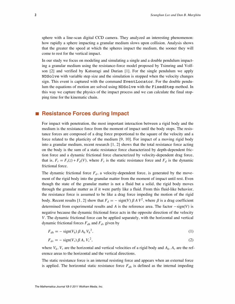
A single-pendulum impact model is presented in Figure 1. The planar motion of thependulum on impact can be described in a fixed Cartesian coordinate system. The x axis ishorizontal, with the positive sense directed to the right; the z axis is vertical, with thepositive sense directed downward; and the y axis is perpendicular to the plane of motion.The angle between the z axis and the pendulum is denoted by q, the generalized coor-dinate describing this system.

Impact of a Planar Kinematic Chain with Granular Matter 3


Ú Figure 1. A single-pendulum impact model.

The pendulum has mass m, length L, and diameter dc. The pendulum impacts a granularmedium of density r at an initial impact angle q0. Gravitational acceleration is g. Here arethe numerical values for the input data.

m = 10;L = 0.5;dc = 0.0254;r = 2.46 µ 10^3;q0 = 30 Pi ê 180;g = 9.8;

The gravitational force acts at the center of mass C of the pendulum. This is the positionvector from the origin O to C.

rC = 8L ê 2 Sin@q@tDD, 0, L ê 2 Cos@q@tDD<;

The resistance force of the granular media is assumed to act at the point E, the center ofthe immersed part of the pendulum. The immersed depth is zT as shown in Figure 1. Thelength LE is the distance from the origin O to E.

zT = L Cos@q@tDD - L Cos@q0D;LE = L - 0.5 zT ê Cos@q@tDD;

These are the position vector and the velocity of the point E.

rE = 8LE Sin@q@tDD, 0, LE Cos@q@tDD<;VE = Cross@D@80, q@tD, 0<, tD, rED;

This is the gravitational force acting at C.

G = 80, 0, m g<;

We use NDSolve to solve the differential equations of motion. The expressions for the re-sistant forces given by equations (1) to (4) contain the signs of the vertical and horizontalvelocities of the application point E. We want to use a variable step size for the integrationfor this model, so we cannot use the Mathematica function Sign. (The function Signcan be used with NDSolve with the FixedStep method; see the double-pendulum ex-ample.) Therefore for the case of the single pendulum we introduce the piecewise-con-stant variables sgnVh and sgnVv, defined in the following lists.



We use NDSolve to solve the differential equations of motion. The expressions for the re-

velocities of the application point E. We want to use a variable step size for the integrationfor this model, so we cannot use the Mathematica function Sign. (The function Signcan be used with NDSolve with the FixedStep method; see the double-pendulum ex-ample.) Therefore for the case of the single pendulum we introduce the piecewise-con-stant variables sgnVh and sgnVv, defined in the following lists.

data1 = 8sgnVh Ø -1, sgnVv Ø 1, b Ø 1569.7, hh Ø 2.43,hv Ø 10, l Ø 1.4<;

data2 = 8sgnVh Ø -1, sgnVv Ø -1, b Ø 1569.7, hh Ø 2.43,hv Ø .5, l Ø 1.7<;

The list data1 is used for plunging (Vv > 0) and the list data2 is used for withdrawing(Vv < 0). For the two lists we consider continuous sliding on the horizontal direction. Thegeneral coefficients for the resistant force [1, 3, 8] are b = 1569.7 and hh = 2.43. Forplunging motion hv = 10, l = 1.4 and for withdrawing motion hv = 0.5, l = 1.7. Whenthe pendulum penetrates the granular medium with plunging motion (0 < q § q0), the val-ues of sgnVh and sgnVv are -1 and 1. When the pendulum withdraws from the granularmedium (q < 0), the values of sgnVh and sgnVv are -1 and -1.

This defines the reference area Ah and the horizontal dynamic frictional force Fd h.

Ah = dc zT;Fdh = -sgnVh b Ah VE@@1DD^2;

Here are the reference area Av and the vertical dynamic frictional force Fd v.

Av = dc zT Abs@Tan@q@tDDD;Fdv = -sgnVv b Av VE@@3DD^2;

Here is the horizontal static resistance force.

Fsh = -sgnVh hh r g dc zT^2 ;

Here are the immersed volume U of the pendulum and the vertical dynamic frictionalforce Fs v.

U = zT ê Cos@q@tDD dc^2 Pi ê 4;Fsv = -sgnVv hv HzT ê dcL^l g r U;

This defines the resistance force.

Fr = 8Fdh + Fsh, 0, Fdv + Fsv<;

The equation of motion of the pendulum is

(5)IO q.. HrCäG+ rEäFrL ÿ H0, 1, 0L.



IO = m ê 3 HL^2L;Eq5 = IO q''@tD == HCross@rC, GD + Cross@rE, FrDL@@2DD;

Here IO is the mass moment inertia about the origin O. The ODE, equation (5), is solvedin single. The input variable dq is the initial impact angular velocity of the pendulum.The initial start time t0, the initial impact angle q0, and the initial impact angular veloc-ity dq0 are defined as initial values. The interpolating function sol, which is the solutionof the ODE, is defined as a local symbol. To save the solution data for the angle q and forthe angular velocity q£, we introduce initially the empty vectors qresults anddqresults. The simulation is performed until the angular velocity q£ becomes zero(considering a numerical error) using the While statement. At the first loop the ODEuses the coefficients list data1 for the plunging motion. NDSolve solves this ODE untilthe z directional velocity VEz of the point E becomes zero and the event is identified usingthe EventLocator method. This event occurs when q£ is zero or when VEz changessign at q = 0. We do not consider the x velocity, VEx, of the point E because the sign ofthe velocity VEx does not change until the angular velocity q£ becomes zero. OnceNDSolve stops solving the ODE, the stopping time is saved as tend. The last values ofthe angle q and the angular velocity q£ of the stopping time, tend, are saved as the initialvalues q0 and dq0 for the next loop. The Table saves the data of the angle q and the an-gular velocity q£ using qresult and dqresult. After saving the data, the new initialstart time t0 of the next loop is defined as the stopping time tend and the motion indexincreases from the plunging motion to the withdrawing motion. After the end of the firstloop, the While statement checks the last value of the angular velocity and decideswhether to do one more loop of calculation or to end the module.

single@dq_D := ModuleA8t0 = 0, q0 = q0, dq0 = dq, sol<,

qresults = 8<; dqresults = 8<; motion = 1;

WhileAChopAdq0, 10-6E != 0,

Eq50 = Eq5 ê. Which@motion == 1, data1, motion == 2, data2D;

sol = NDSolve@8Eq50, q@t0D ã q0, q£@t0D ã dq0<, q,8t, t0, Infinity<, MaxSteps Ø Infinity,Method Ø 8"EventLocator", "Event" Ø VE@@3DD,

"EventAction" ß Throw@tend = t; q0 = q@tD;dq0 = q'@tD;, "StopIntegration"D,

"EventLocationMethod" Ø "LinearInterpolation","Method" Ø "ExplicitEuler"<D;

qresult = Table@8t, q@tD 180 ê Pi ê. sol@@1DD<,8t, t0, tend, .0025<D;

dqresult = Table@8t, q'@tD ê. sol@@1DD<,8t, t0, tend, .0025<D;

qresults = Append@qresults, qresultD;;



qresults = Append@qresults, qresultD;dqresults = Append@dqresults, dqresultD;

t0 = tend;motion++E H* end While *L

E H* end Module *L

The simulation of the model is performed for an initial impact angle q0 = 30 ° and forthree initial impact angular velocities (q° 0 = -3, -1.5, and -0.1 rad/s). The angle q andthe angular velocity q° are plotted with the blue line for q° 0 =-3 rad/s, the red dashed linefor -1.5 rad/s, and the black dot-dashed line for -0.1 rad/s.

single@-3D;PrintA"The stopping time for q°0 = -3 radês is ",

tend, " @sD"E;

qplot1 = ListLinePlot@qresults, PlotRange Ø Full,PlotStyle Ø 8Directive@BlueD<D;

dqplot1 = ListLinePlot@dqresults, PlotRange Ø Full,PlotStyle Ø 8Directive@BlueD<D;

[email protected];PrintA"The stopping time for q°0 = -1.5 radês is ",

tend, " @sD"E;

qplot2 = ListLinePlot@qresults, PlotRange Ø Full,PlotStyle Ø 8Directive@8Red, Dashed<D<D;

dqplot2 = ListLinePlot@dqresults, PlotRange Ø Full,PlotStyle Ø 8Directive@8Red, Dashed<D<D;

[email protected];PrintA"The stopping time for q°0 = -0.1 radês is ",

tend, " @sD"E;

qplot3 = ListLinePlot@qresults, PlotRange Ø Full,PlotStyle Ø 8Directive@8Black, DotDashed<D<D;

dqplot3 = ListLinePlot@dqresults, PlotRange Ø Full,PlotStyle Ø 8Directive@8Black, DotDashed<D<D;

Show@qplot1, qplot2, qplot3, Frame Ø True,FrameLabel Ø 8"time @sD", "q @°D"<,PlotRange Ø 880, tend<, 8-30, 33<<, GridLines Ø AutomaticD

ShowAdqplot1, dqplot2, dqplot3, Frame Ø True,

FrameLabel Ø 9"time @sD", "q° @radêsD"=,

PlotRange Ø 880, tend<, 8-3.8, .2<<, GridLines Ø AutomaticE



The stopping time for q°0 = -3 radês is 0.430259 @sD

The stopping time for q°0 = -1.5 radês is 0.474437 @sD

The stopping time for q°0 = -0.1 radês is 0.553072 @sD

0.0 0.1 0.2 0.3 0.4 0.5-30

-20

-10

0

10

20

30

time @sD

q@°D

0.0 0.1 0.2 0.3 0.4 0.5

-3

-2

-1

0

time @sD

q°@ra

dêsD

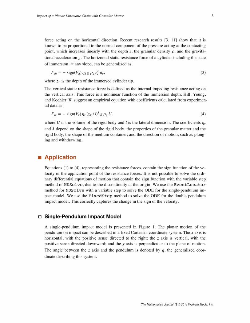
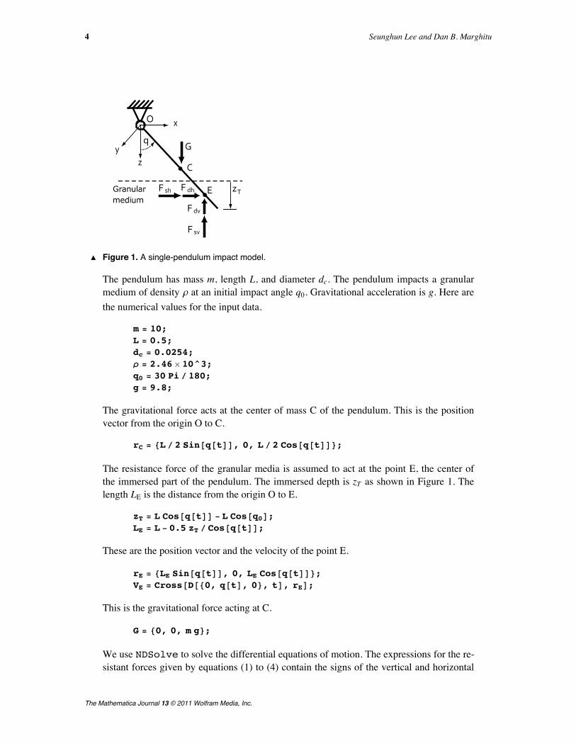
The simulation results of the model for the initial impact angle q0 = 30 ° show that whenthe initial impact velocity of the pendulum increases, the penetrating angle increases. How-ever, we observed the stopping time, defined as duration from the moment of impact untilthe angular velocity becomes zero, decreases: for q° 0 = -3 rad/s the stopping time is0.430259 s, for q° 0 = -1.5 rad/s the stopping time is 0.474437 s, and for q° 0 = -0.1 rad/sthe stopping time is 0.553072 s.



· Double-Pendulum Impact Model

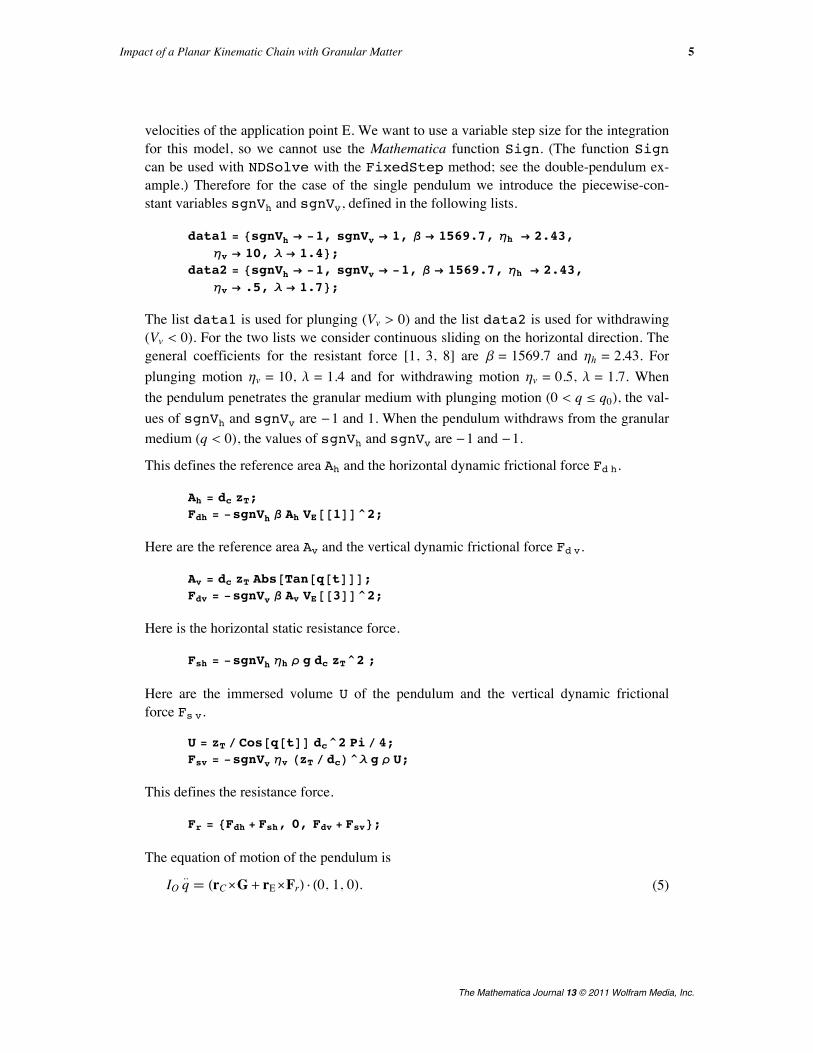
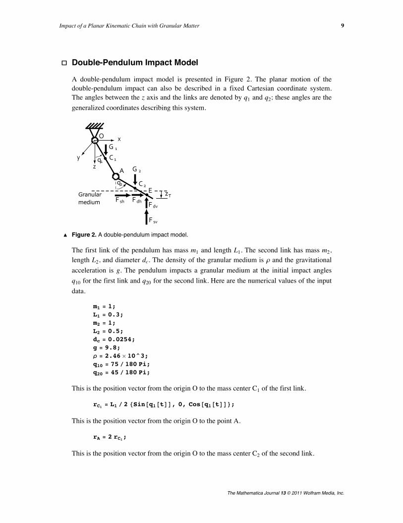
A double-pendulum impact model is presented in Figure 2. The planar motion of thedouble-pendulum impact can also be described in a fixed Cartesian coordinate system.The angles between the z axis and the links are denoted by q1 and q2; these angles are thegeneralized coordinates describing this system.

Ú Figure 2. A double-pendulum impact model.

The first link of the pendulum has mass m1 and length L1. The second link has mass m2,length L2, and diameter dc. The density of the granular medium is r and the gravitationalacceleration is g. The pendulum impacts a granular medium at the initial impact anglesq10 for the first link and q20 for the second link. Here are the numerical values of the inputdata.

m1 = 1;L1 = 0.3;m2 = 1;L2 = 0.5;dc = 0.0254;g = 9.8;r = 2.46 µ 10^3;q10 = 75 ê 180 Pi;q20 = 45 ê 180 Pi;

This is the position vector from the origin O to the mass center C1 of the first link.

rC1 = L1 ê 2 8Sin@q1@tDD, 0, Cos@q1@tDD<;

This is the position vector from the origin O to the point A.

rA = 2 rC1;

This is the position vector from the origin O to the mass center C2 of the second link.



rC2 = rA + L2 ê 2 8Sin@q2@tDD, 0, Cos@q2@tDD<;

Here is the acceleration vector of the position vector.

aC2 = D@rC2, 8t, 2<D;

We calculate the immersed depth zT and the length LE.

zT = L1 Cos@q1@tDD + L2 Cos@q2@tDD - HL1 Cos@q10D + L2 Cos@q20DL;LE = L2 - 0.5 zT ê Cos@q2@tDD;

Here are the position vector and the velocity of the force application point E.

rE = rA + LE 8Sin@q2@tDD, 0, Cos@q2@tDD<;VE = D@rA, tD + Cross@D@80, q2@tD, 0<, tD, HrE - rALD;

These are the gravitational forces acting at C1 and C2.

G1 = 80, 0, m1 g<;G2 = 80, 0, m2 g<;

The function Sign can be used with NDSolve with the FixedStep method as men-tioned previously. Therefore, we define the horizontal dynamic frictional force.

b = 1569.7;Fdh = -Sign@VE@@1DDD b dc zT VE@@1DD^2;

Here is the vertical dynamic frictional force.

Fdv = -Sign@VE@@3DDD b dc zT Abs@Tan@q2@tDDD VE@@3DD^2;

Here is the horizontal static resistance force.

hh = 2.43;Fsh = -Sign@VE@@1DDD hh r g dc zT^2;

We express the vertical resistance force coefficients, hv = 10 and l = 1.4 for plunging mo-tion, hv = 0.5 and l = 1.7 for withdrawing motion.

hv = Piecewise@8810, VE@@3DD > 0<, 80.5, VE@@3DD < 0<<D;l = [email protected], VE@@3DD > 0<, 81.7, VE@@3DD < 0<<D;

This is the vertical static resistance force.

Fsv = -Sign@VE@@3DDD hv HzT ê dcL^l g r zT ê Cos@q2@tDD dc^2 Pi ê 4;

This is the resistance force.



Fr = 8Fdh + Fsh, 0, Fdv + Fsv<;

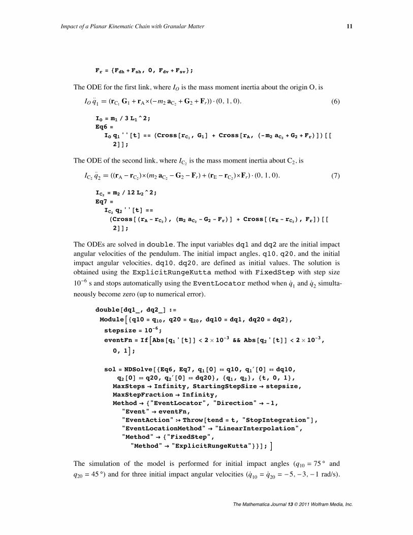
The ODE for the first link, where IO is the mass moment inertia about the origin O, is

(6)IO q..1 HrC1 G1 + rAäH-m2 aC2 +G2 + FrLL ÿ H0, 1, 0L.

IO = m1 ê 3 L1^2;Eq6 =

IO q1''@tD == HCross@rC1, G1D + Cross@rA, H-m2 aC2 + G2 + FrLDL@@2DD;

The ODE of the second link, where IC2 is the mass moment inertia about C2, is

(7)IC2 q..2 HHrA - rC2LäHm2 aC2 -G2 - FrL+ HrE - rC2LäFrL ÿ H0, 1, 0L.

IC2 = m2 ê 12 L2^2;Eq7 =

IC2 q2''@tD ==

HCross@HrA - rC2L, Hm2 aC2 - G2 - FrLD + Cross@HrE - rC2L, FrDL@@2DD;

The ODEs are solved in double. The input variables dq1 and dq2 are the initial impactangular velocities of the pendulum. The initial impact angles, q10, q20, and the initialimpact angular velocities, dq10, dq20, are defined as initial values. The solution isobtained using the ExplicitRungeKutta method with FixedStep with step size10-6 s and stops automatically using the EventLocator method when q° 1 and q° 2 simulta-neously become zero (up to numerical error).

double@dq1_, dq2_D :=ModuleA8q10 = q10, q20 = q20, dq10 = dq1, dq20 = dq2<,

stepsize = 10-6;eventFn = IfAAbs@q1'@tDD < 2 µ 10-3 && Abs@q2'@tDD < 2 µ 10-3,

0, 1E;

sol = NDSolve@8Eq6, Eq7, q1@0D ã q10, q1£@0D ã dq10,q2@0D ã q20, q2£@0D ã dq20<, 8q1, q2<, 8t, 0, 1<,

MaxSteps Ø Infinity, StartingStepSize Ø stepsize,MaxStepFraction Ø Infinity,Method Ø 8"EventLocator", "Direction" Ø -1,

"Event" Ø eventFn,"EventAction" ß Throw@tend = t, "StopIntegration"D,"EventLocationMethod" Ø "LinearInterpolation","Method" Ø 8"FixedStep",

"Method" Ø "ExplicitRungeKutta"<<D; E

The simulation of the model is performed for initial impact angles (q10 = 75 ° andq20 = 45 °) and for three initial impact angular velocities (q° 10 = q° 20 = -5, -3, -1 rad/s).The angle q and the angular velocity q° are plotted in blue for q° 10 = q° 20 = -5 rad/s, reddashed for -3 rad/s, and black dot-dashed for -1 rad/s.



The simulation of the model is performed for initial impact angles (q10 = 75 ° andq20 = 45 °) and for three initial impact angular velocities (q° 10 = q° 20 = -5, -3, -1 rad/s).The angle q and the angular velocity q° are plotted in blue for q° 10 = q° 20 = -5 rad/s, reddashed for -3 rad/s, and black dot-dashed for -1 rad/s.

double@-5, -5D;PrintA"The stopping time for q°10 = q°20 = -5 radês is ",

tend, " @sD"E;

SetOptions@Plot, PlotRange Ø Full, PlotStyle Ø BlueD;q1plot1 = Plot@Evaluate@q1@tD 180 ê Pi ê. solD, 8t, 0, tend<D;q2plot1 = Plot@Evaluate@q2@tD 180 ê Pi ê. solD, 8t, 0, tend<D;dq1plot1 = Plot@Evaluate@q1'@tD ê. solD, 8t, 0, tend<D;dq2plot1 = Plot@Evaluate@q2'@tD ê. solD, 8t, 0, tend<D;


tend, " @sD"E;

SetOptions@Plot, PlotRange Ø Full, PlotStyle Ø 8Red, Dashed<D;q1plot2 = Plot@Evaluate@q1@tD 180 ê Pi ê. solD, 8t, 0, tend<D;q2plot2 = Plot@Evaluate@q2@tD 180 ê Pi ê. solD, 8t, 0, tend<D;dq1plot2 = Plot@Evaluate@q1'@tD ê. solD, 8t, 0, tend<D;dq2plot2 = Plot@Evaluate@q2'@tD ê. solD, 8t, 0, tend<D;


tend, " @sD"E;

SetOptions@Plot, PlotRange Ø Full,PlotStyle Ø 8Black, DotDashed<D;

q1plot3 = Plot@Evaluate@q1@tD 180 ê Pi ê. solD, 8t, 0, tend<D;q2plot3 = Plot@Evaluate@q2@tD 180 ê Pi ê. solD, 8t, 0, tend<D;dq1plot3 = Plot@Evaluate@q1'@tD ê. solD, 8t, 0, tend<D;dq2plot3 = Plot@Evaluate@q2'@tD ê. solD, 8t, 0, tend<D;

Show@q1plot1, q1plot2, q1plot3, Frame Ø True,FrameLabel Ø 8"time @sD", "q1 @°D"<,PlotRange Ø 880, tend<, 8-44, 80<<, GridLines Ø AutomaticD

Show@q2plot1, q2plot2, q2plot3, Frame Ø True,FrameLabel Ø 8"time @sD", "q2 @°D"<,PlotRange Ø 880, tend<, 840, 72<<, GridLines Ø AutomaticD

ShowAdq1plot1, dq1plot2, dq1plot3, Frame Ø True,

FrameLabel Ø 9"time @sD", "q°1 @radêsD"=,

PlotRange Ø 880, tend<, 8-9, 0.4<<, GridLines Ø AutomaticE

ShowAdq2plot1, dq2plot2, dq2plot3, Frame Ø True,

FrameLabel Ø 9"time @sD", "q°2 @radêsD"=,

PlotRange Ø 880, tend<, 8-5.5, 7<<, GridLines Ø AutomaticE



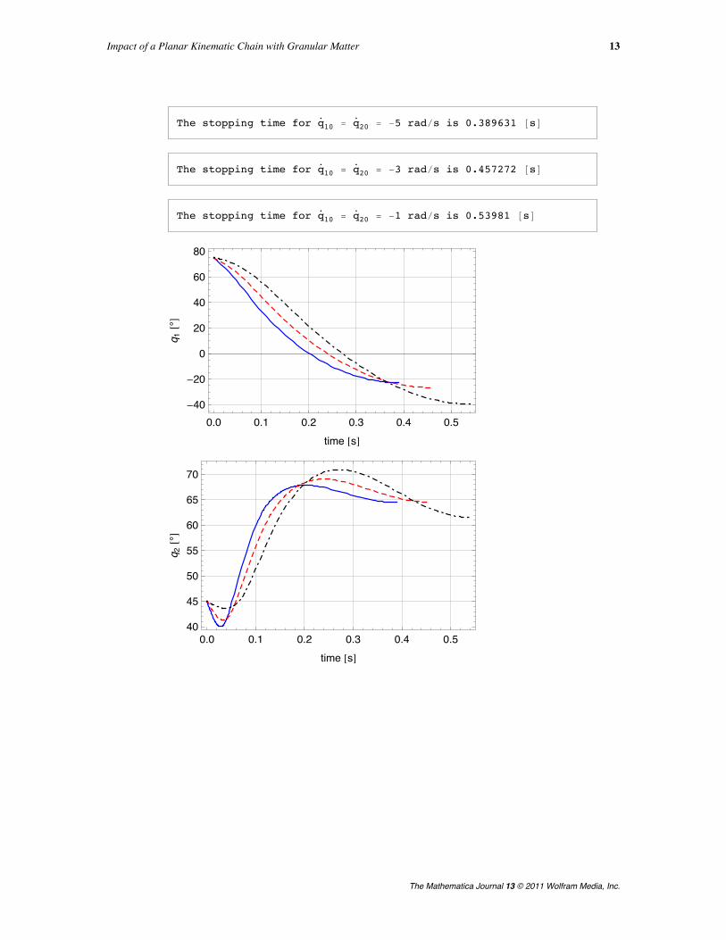
The stopping time for q°10 = q

°20 = -5 radês is 0.389631 @sD


°20 = -3 radês is 0.457272 @sD


°20 = -1 radês is 0.53981 @sD

0.0 0.1 0.2 0.3 0.4 0.5-40

-20

0

20

40

60

80

time @sD

q 1@°D

0.0 0.1 0.2 0.3 0.4 0.540

45

50

55

60

65

70

time @sD

q 2@°D



0.0 0.1 0.2 0.3 0.4 0.5

-8

-6

-4

-2

0

time @sD

q° 1@ra

dêsD

0.0 0.1 0.2 0.3 0.4 0.5

-4

-2

0

2

4

6

time @sD

q° 2@ra

dêsD

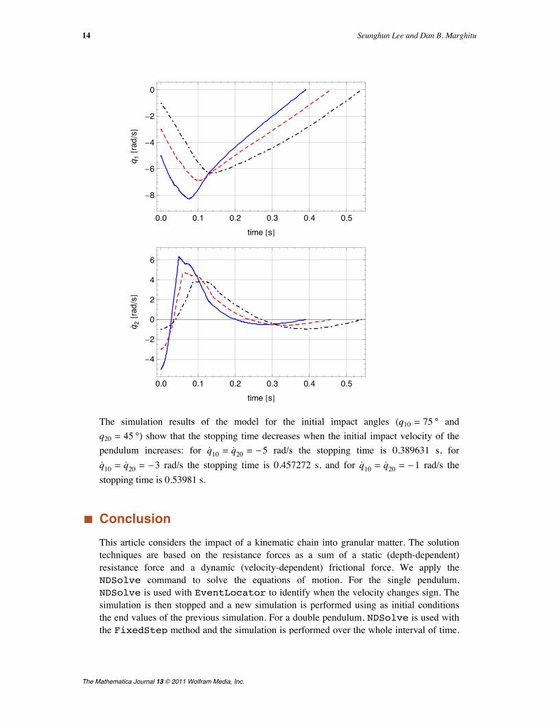
The simulation results of the model for the initial impact angles (q10 = 75 ° andq20 = 45 °) show that the stopping time decreases when the initial impact velocity of thependulum increases: for q° 10 = q° 20 = -5 rad/s the stopping time is 0.389631 s, forq° 10 = q° 20 = -3 rad/s the stopping time is 0.457272 s, and for q° 10 = q° 20 = -1 rad/s thestopping time is 0.53981 s.

‡ ConclusionThis article considers the impact of a kinematic chain into granular matter. The solutiontechniques are based on the resistance forces as a sum of a static (depth-dependent)resistance force and a dynamic (velocity-dependent) frictional force. We apply theNDSolve command to solve the equations of motion. For the single pendulum,NDSolve is used with EventLocator to identify when the velocity changes sign. Thesimulation is then stopped and a new simulation is performed using as initial conditionsthe end values of the previous simulation. For a double pendulum, NDSolve is used withthe FixedStep method and the simulation is performed over the whole interval of time.We observe that the numerical solution leads to a seemingly paradoxical result: as theinitial velocity increases, the stopping time decreases.



This article considers the impact of a kinematic chain into granular matter. The solutiontechniques are based on the resistance forces as a sum of a static (depth-dependent)resistance force and a dynamic (velocity-dependent) frictional force. We apply theNDSolve command to solve the equations of motion. For the single pendulum,NDSolve is used with EventLocator to identify when the velocity changes sign. Thesimulation is then stopped and a new simulation is performed using as initial conditionsthe end values of the previous simulation. For a double pendulum, NDSolve is used with

We observe that the numerical solution leads to a seemingly paradoxical result: as theinitial velocity increases, the stopping time decreases.

‡ AcknowledgmentsFor this work we used Mathematica 7.0.1 and a Intel Core Duo computer running Mac OSX with a 2.0 GHz CPU and 2 GB of RAM.

‡ References[1] H. Katsuragi and D. J. Durian, “Unified Force Law for Granular Impact Cratering,” Nature

Physics, 3, 2007 pp. 420–423. www.nature.com/nphys/journal/v3/n6/full/nphys583.html.

[2] L. S. Tsimring and D. Volfson, “Modeling of Impact Cratering in Granular Media,” in Powdersand Grains 2005, Proceedings of International Conference on Powders & Grains 2005 (R.García-Rojo, H. J. Herrmann, and S. McNamara, eds.), London: Taylor & Francis, 2005pp. 1215–1218.

[3] R. Albert, M. A. Pfeifer, A.-L. Barabási, and P. Schiffer, “Slow Drag in a Granular Medium,”Physical Review Letters, 82(1), 1999 pp. 205–208.www.prl.aps.org/abstract/PRL/v82/i1/p205_1.

[4] I. Albert, P. Tegzes, B. Kahng, R. Albert, J. G. Sample, M. Pfeifer, A.-L. Barabási, T. Vicsek,and P. Schiffer, “Jamming and Fluctuations in Granular Drag,” Physical Review Letters, 84,2000 pp. 5122–5125. arxiv.org/abs/cond-mat/9912336.

[5] I. Albert, P. Tegzes, R. Albert, J. G. Sample, A.-L. Barabási, T. Vicsek, B. Kahng, and P.Schiffer, “Stick-Slip Fluctuations in Granular Drag,” Physical Review E, 64, 2001 031307(9).arxiv.org/abs/cond-mat/0102523.

[6] I. Albert, J. G. Sample, A. J. Morss, S. Rajagopalan, A.-L. Barabási, and P. Schiffer,“Granular Drag on a Discrete Object: Shape Effects on Jamming,” Physical Review E, 64,2001 061303(4). arxiv.org/abs/cond-mat/0107392.

[7] M. B. Stone, R. Barry, D. P. Bernstein, M. D. Pelc, Y. K. Tsui, and P. Schiffer, “Studies of Lo-cal Jamming via Penetration of a Granular Medium,” Physical Review E, 70, 2004041301(10). arxiv.org/abs/cond-mat/0404587.

[8] G. Hill, S. Yeung, and S. A. Koehler, “Scaling Vertical Drag Forces in Granular Media,” Euro-physics Letters, 72(1), 2005 pp. 137–142. www.iopscience.iop.org/0295-5075/72/1/137.

[9] A. L. Yarin, M. B. Rubin, and I. V. Roisman, “Penetration of a Rigid Projectile into an Elastic-Plastic Target of Finite Thickness,” International Journal of Impact Engineering, 16(5), 1995pp. 801–831. www.sciencedirect.com/science/article/pii/0734743X95000197.

[10] G. Yossifon, A. L. Yarin, and M. B. Rubin, “Penetration of a Rigid Projectile into a Multi-Lay-ered Target: Theory and Numerical Computations,” International Journal of Engineering Sci-ence, 40(12), 2002 pp. 1381–1401. doi:10.1016/S0020-7225(02)00013-7.

[11] S. N. Coppersmith, C.-H. Liu, S. Majumdar, O. Narayan, and T. A. Witten, “A Model forForce Fluctuations in Bead Packs,” Physical Review E, 53(5), 1996 pp. 4673–4685.www.arxiv.org/abs/cond-mat/9511105.

S. Lee and D. B. Marghitu, “Impact of a Planar Kinematic Chain with Granular Matter,” The Mathematica Jour-nal, 2011. dx.doi.org/doi:10.3888/tmj.13–2.



About the Authors

Seunghun Lee was a Ph.D. student in the mechanical engineering department at AuburnUniversity, studying theoretical modeling of robotic systems. He is now serving in the Ko-rean army.Dan B. Marghitu is a professor of mechanical engineering at Auburn University. His re-search areas are impact dynamics, mechanisms, robots, and nonlinear dynamics.Mechanical Engineering Dept.Auburn University 270 Ross Hall, Auburn, AL [email protected]@auburn.edu



Documents

The Mathematica Journal Impact of a Planar Kinematic Chain with