Embed Size (px)
Citation preview
• The market demand curve.
• Utility and the demand curve.
• Consumer surplus.
• The determinants of demand.
• The classification of goods.
• Concepts of elasticity.
• The relationship between price elasticity and
sales revenue.
CHAPTER 2. The analysis of consumer demand
OHT 2.1
This chapter will help you to:• Understand why changes in price affect consumer demand and, in
particular, why demand curves are normally downward sloping, i.e. the law of demand.
• Understand why demand curves may shift in response to changes in various factors, other than price, which impact upon demand (known as the conditions of demand).
• Analyse the nature of the relationship between marginal utility and the demand curve for any product or service.
• Appreciate the meaning and importance of consumer surplus in the context of pricing strategies.
Learning outcomes OHT 2.2A

• Interpret the relative importance of income and substitution effects on demand when the price of a good or service changes.
• Classify goods and services according to how demand responds to changes in price and income, giving rise to the terms normal, inferior, Giffen and Veblen goods or services.
• Calculate price, cross-price and income elasticities of demand and interpret the significance of the results.
• Appreciate the relationship between price elasticity, marginal revenue and total revenue arising from the sale of goods or services.
OHT 2.2BLearning outcomes
A consumer’s demand curve relates the amount the consumer is willing to buy to each conceivable price for the product.
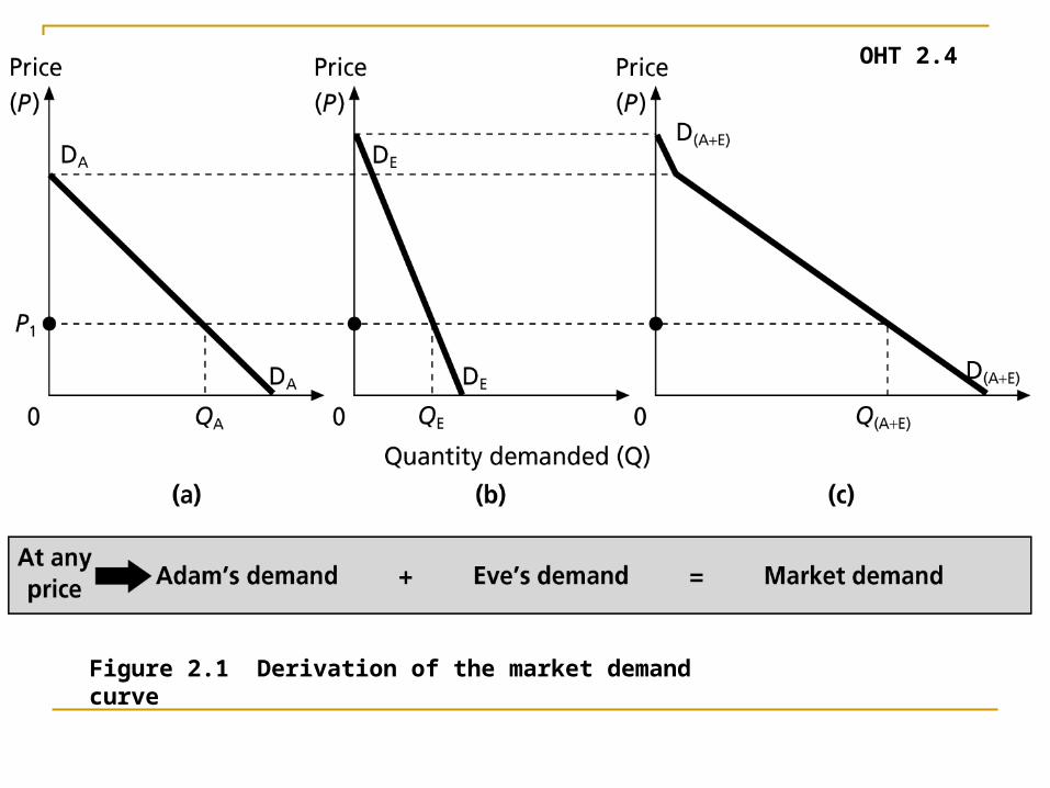
The market demand curve for a good or service is derived by summing the individual demand curves of consumers horizontally for any given price.
The market demand curveOHT 2.3
OHT 2.4
Figure 2.1 Derivation of the market demand curve
In general there is a central law of demand, which states that there is an inverse relationship between the price of a good and the quantity demanded assuming all other factors that might influence demand are held constant .
The law of demandOHT 2.5
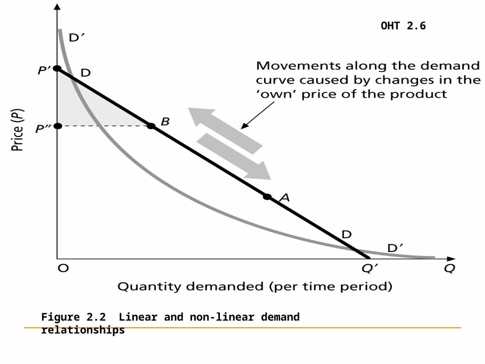
OHT 2.6
Figure 2.2 Linear and non-linear demand relationships
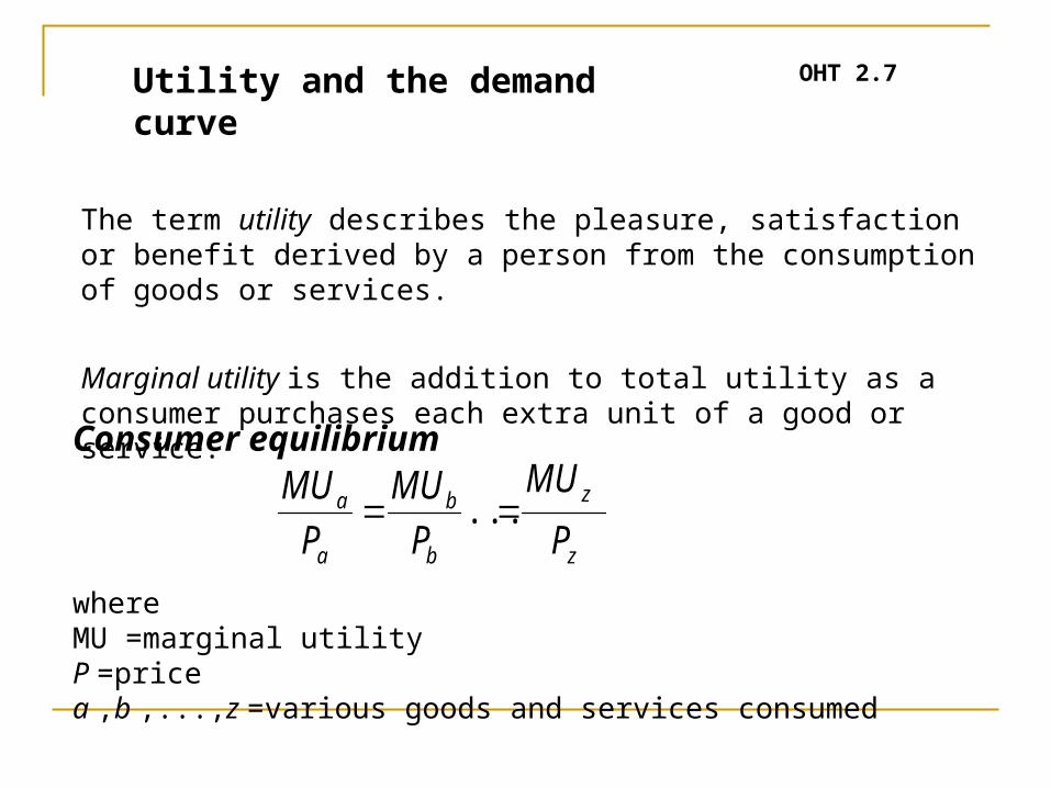
Consumer equilibrium
whereMU =marginal utilityP =pricea ,b ,...,z =various goods and services consumed
The term utility describes the pleasure, satisfaction or benefit derived by a person from the consumption of goods or services.
Marginal utility is the addition to total utility as a consumer purchases each extra unit of a good or service.
Utility and the demand curve OHT 2.7
z
z
b
b
a
a
P
MU
P
MU
P
MU ...
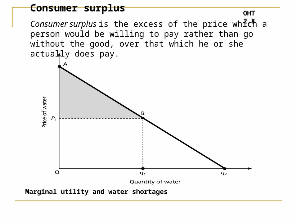
OHT 2.8
Marginal utility and water shortages
Consumer surplus
Consumer surplus is the excess of the price which a person would be willing to pay rather than go without the good, over that which he or she actually does pay.
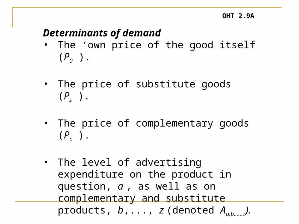
Determinants of demand• The ‘own price of the good itself (P0 ).
• The price of substitute goods (Ps ).
• The price of complementary goods (Pc ).
• The level of advertising expenditure on the product in question, a , as well as on complementary and substitute products, b,..., z (denoted Aa,b,…..z).
• The level and distribution of consumers disposable incomes (Yd ),i.e.income after state direct taxes and benefits.
OHT 2.9A
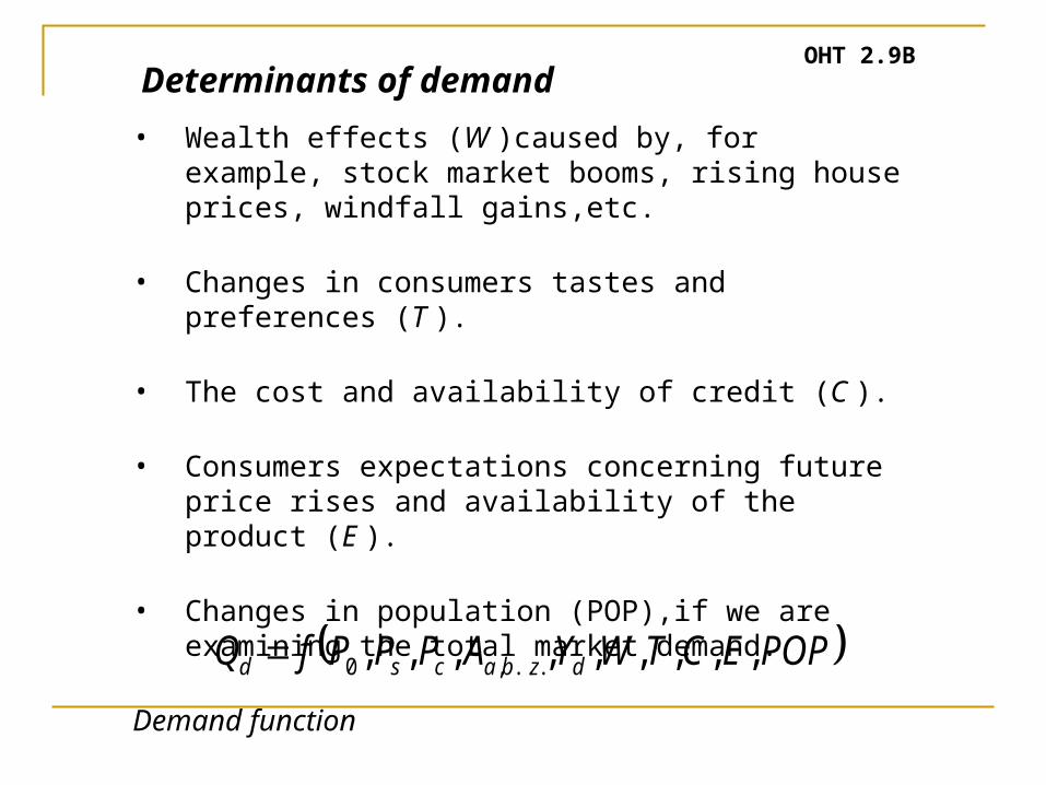
• Wealth effects (W )caused by, for example, stock market booms, rising house prices, windfall gains,etc.
• Changes in consumers tastes and preferences (T ).
• The cost and availability of credit (C ).
• Consumers expectations concerning future price rises and availability of the product (E ).
• Changes in population (POP),if we are examining the total market demand.
Demand function
OHT 2.9BDeterminants of demand
POPECTWYAPPPfQ dzbacsd ,,,,,,,,, ...,0
OHT 2.10
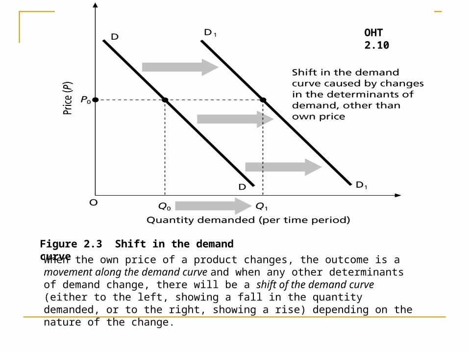
Figure 2.3 Shift in the demand curve
When the own price of a product changes, the outcome is a movement along the demand curve and when any other determinants of demand change, there will be a shift of the demand curve (either to the left, showing a fall in the quantity demanded, or to the right, showing a rise) depending on the nature of the change.
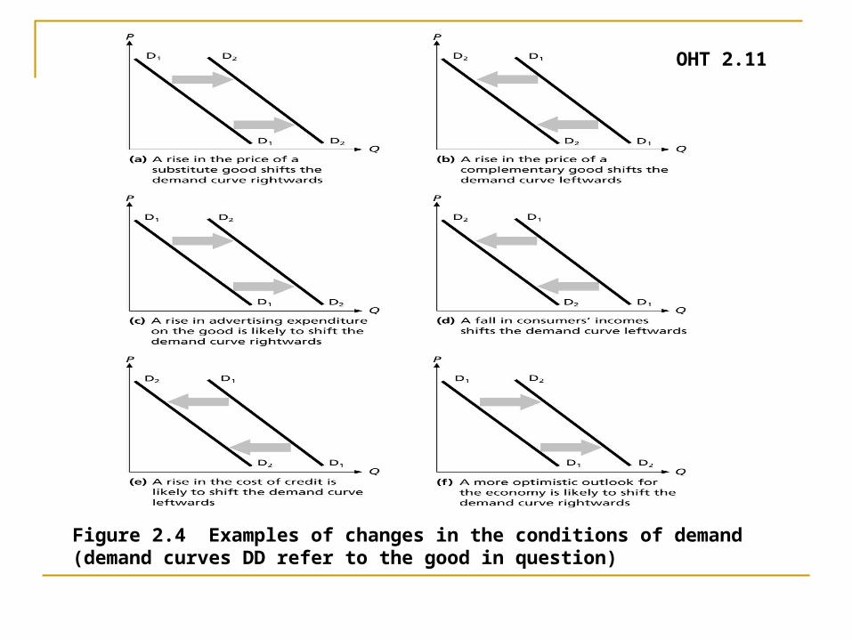
OHT 2.11
Figure 2.4 Examples of changes in the conditions of demand (demand curves DD refer to the good in question)
• Normal products.
• Inferior products.
• Giffen products.
• Veblen products.
Classification of productsOHT 2.12
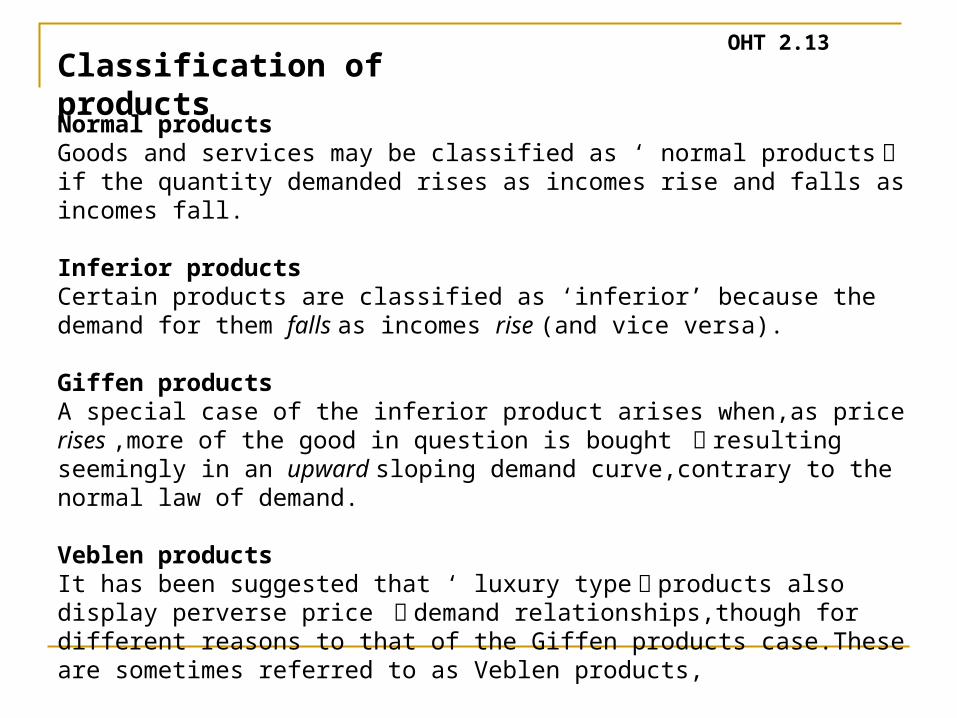
Normal productsGoods and services may be classified as ‘ normal products 段 if the quantity demanded rises as incomes rise and falls as incomes fall.
Inferior productsCertain products are classified as ‘inferior’ because the demand for them falls as incomes rise (and vice versa).
Giffen productsA special case of the inferior product arises when,as price rises ,more of the good in question is bought 睦 resulting seemingly in an upward sloping demand curve,contrary to the normal law of demand.
Veblen productsIt has been suggested that ‘ luxury type 恥 products also display perverse price 謀 demand relationships,though for different reasons to that of the Giffen products case.These are sometimes referred to as Veblen products,
OHT 2.13Classification of products
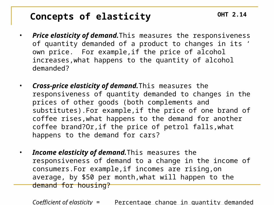
• Price elasticity of demand.This measures the responsiveness of quantity demanded of a product to changes in its ‘ own price. For example,if the price of alcohol increases,what happens to the quantity of alcohol demanded?
• Cross-price elasticity of demand.This measures the responsiveness of quantity demanded to changes in the prices of other goods (both complements and substitutes).For example,if the price of one brand of coffee rises,what happens to the demand for another coffee brand?Or,if the price of petrol falls,what happens to the demand for cars?
• Income elasticity of demand.This measures the responsiveness of demand to a change in the income of consumers.For example,if incomes are rising,on average, by $50 per month,what will happen to the demand for housing?
Coefficient of elasticity = Percentage change in quantity demandedPercentage change in the relevant variable
OHT 2.14Concepts of elasticity
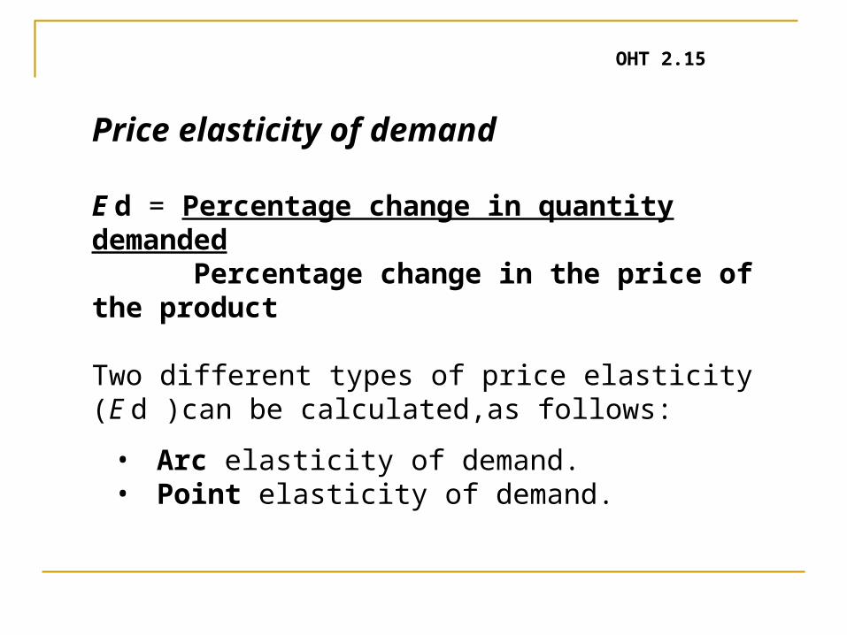
Price elasticity of demand
E d = Percentage change in quantity demanded Percentage change in the price of the product
Two different types of price elasticity (E d )can be calculated,as follows:
• Arc elasticity of demand.• Point elasticity of demand.
OHT 2.15
OHT 2.12
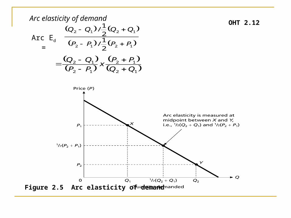
Figure 2.5 Arc elasticity of demand
Arc elasticity of demand
1212
1212
21
/
21
/
PPPP
QQQQ
12
12
12
12
PPx
PP
Arc Ed =
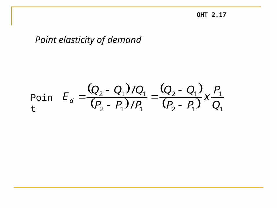
Point elasticity of demand
OHT 2.17
1
1
12
12
112
112
/
/
Q
Px
PP
PPP
QQQEd
Point
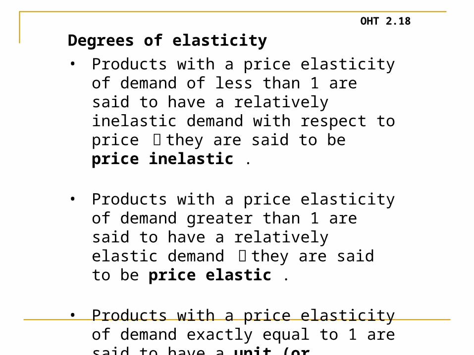
• Products with a price elasticity of demand of less than 1 are said to have a relatively inelastic demand with respect to price 釦they are said to be price inelastic .
• Products with a price elasticity of demand greater than 1 are said to have a relatively elastic demand 釦 they are said to be price elastic .
• Products with a price elasticity of demand exactly equal to 1 are said to have a unit (or unitary)elasticity of demand.
OHT 2.18
Degrees of elasticity
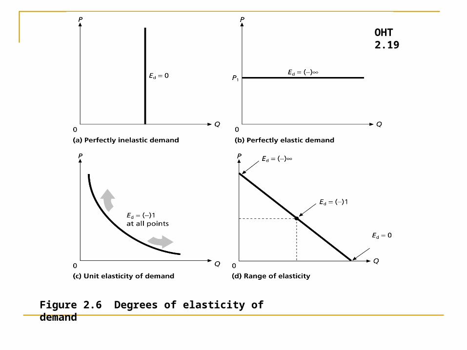
OHT 2.19
Figure 2.6 Degrees of elasticity of demand
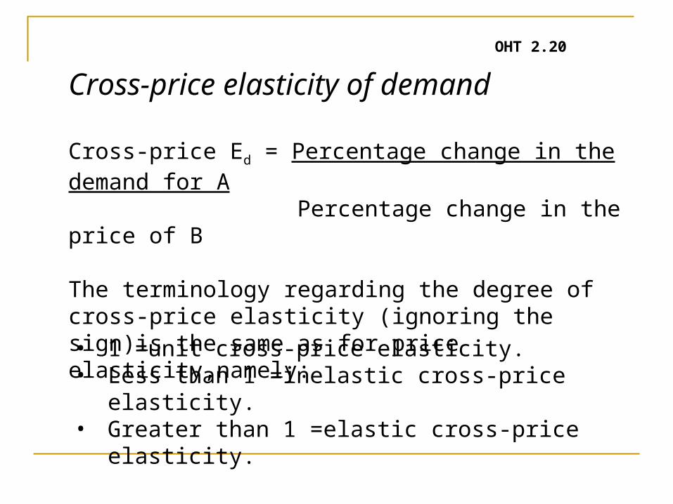
Cross-price elasticity of demand
Cross-price Ed = Percentage change in the demand for A Percentage change in the price of B
The terminology regarding the degree of cross-price elasticity (ignoring the sign)is the same as for price elasticity,namely:
• 1 =unit cross-price elasticity.• Less than 1 =inelastic cross-price elasticity.• Greater than 1 =elastic cross-price elasticity.
OHT 2.20
Income elasticity of demand
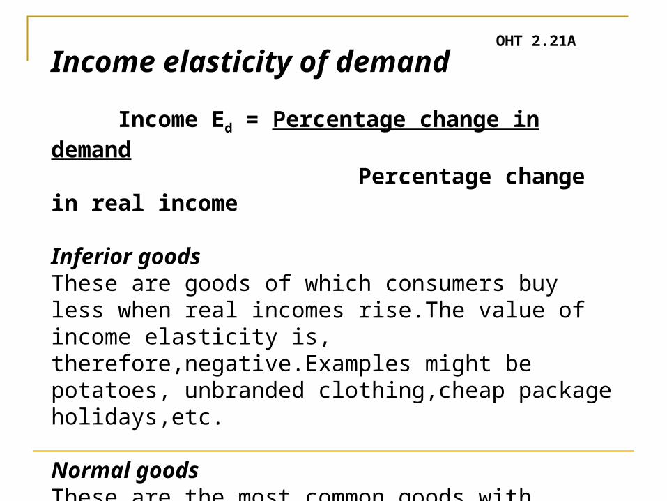
Income Ed = Percentage change in demand Percentage change in real income
Inferior goodsThese are goods of which consumers buy less when real incomes rise.The value of income elasticity is, therefore,negative.Examples might be potatoes, unbranded clothing,cheap package holidays,etc.
Normal goodsThese are the most common goods with demand generally rising as real income rises. They can themselves be further subdivided into two categories:
OHT 2.21A
Necessities .These are goods and services which exhibit a positive income elasticity of demand,though the value will tend to be less than 1. Articles such as basic foodstuffs and ordinary day-to-day clothing fall into this category.Consumers will purchase a certain amount of these goods at very low levels of income,but they will tend for any given percentage increase in real income to increase their spending on the goods by a smaller proportion.
Luxuries . At very low income levels,nothing will be spent on these but,once a certain threshold income level is reached,the proportionate rise in demand for luxury goods is greater than the proportionate rise in real income,e.g.foreign holidays,dining out and DVD players.
OHT 2.21B
OHT 2.22
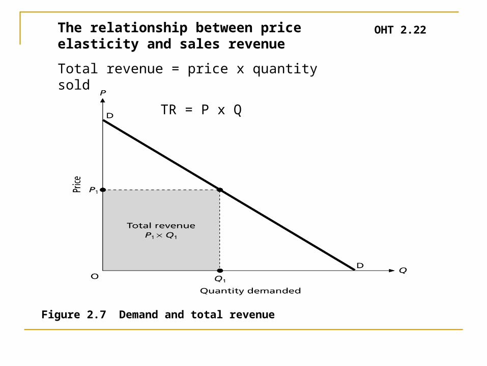
Figure 2.7 Demand and total revenue
The relationship between price elasticity and sales revenue
Total revenue = price x quantity sold
TR = P x Q
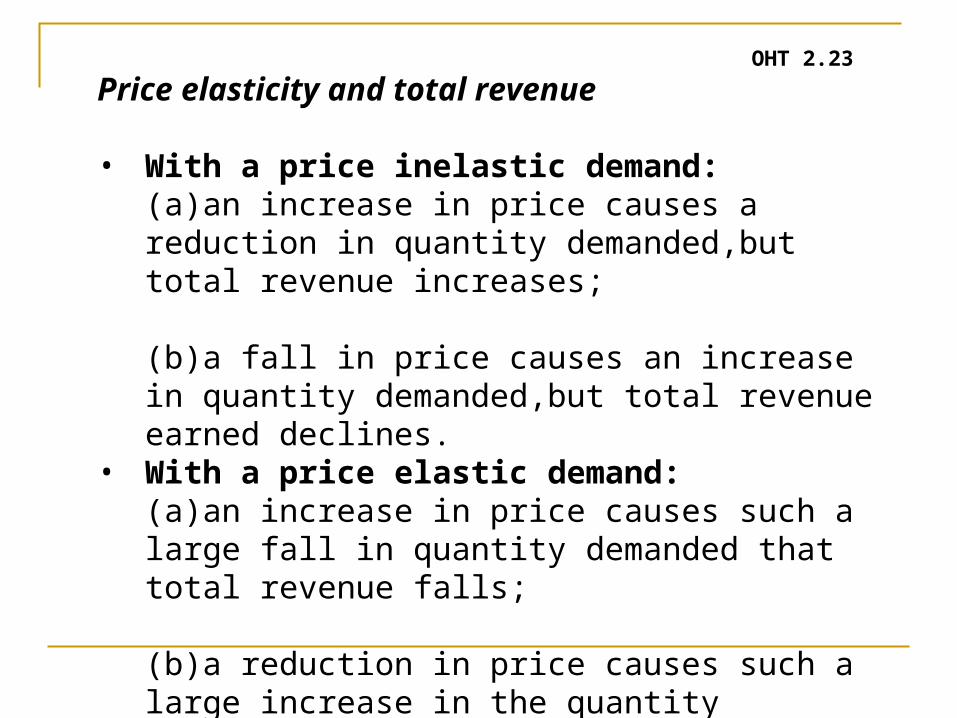
Price elasticity and total revenue
• With a price inelastic demand:(a)an increase in price causes a reduction in quantity demanded,but total revenue increases;
(b)a fall in price causes an increase in quantity demanded,but total revenue earned declines.
• With a price elastic demand:(a)an increase in price causes such a large fall in quantity demanded that total revenue falls;
(b)a reduction in price causes such a large increase in the quantity demanded that the total revenue rises.
OHT 2.23
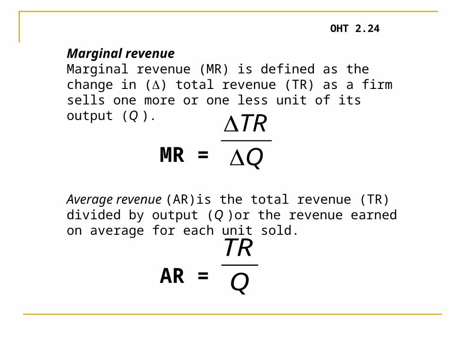
Marginal revenueMarginal revenue (MR) is defined as the change in () total revenue (TR) as a firm sells one more or one less unit of its output (Q ).
MR =
Average revenue (AR)is the total revenue (TR) divided by output (Q )or the revenue earned on average for each unit sold.
AR =
OHT 2.24
Q
TR
Q
TR
OHT 2.25
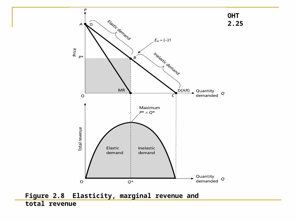
Figure 2.8 Elasticity, marginal revenue and total revenue
• Marginal revenue falls as output rises. Since the demand curve slopes downwards, the addition to total revenue from producing and selling extra units declines.
• Average revenue exceeds marginal revenue. When the demand curve is downward sloping,the marginal revenue from selling one more unit falls faster than the average revenue from selling the total output.
• The marginal revenue curve declines at twice the rate of the demand (average revenue)curve. Hence, the marginal revenue curve cuts the horizontal axis at a point midway between the origin and point C in Figure 2.8.A proof of this mathematical relationship is given in Appendix 2.2 at the end of the chapter.
OHT 2.26A
Elasticity, marginal revenue and total revenue - key relationships
• When total revenue is increasing,marginal revenue is positive. This results from the fact that demand is elastic between points A and B on the demand curve DD in Figure 2.8.
• When total revenue is falling,marginal revenue is negative.A negative marginal revenue results from demand being inelastic between points B and C in Figure 2.8.
• Total revenue is maximised when marginal revenue is zero which occurs when the price elasticity is unitary.Therefore,further attempts to increase total revenue by lowering price below P *will fail because the sales volume will not increase sufficiently to compensate for the price fall.
Elasticity, marginal revenue and total revenue - key relationships
OHT 2.26B
• A demand curve relates the amount that consumers are willing to buy to each conceivable price for the product.
• In general, the law of demand states that there is an inverse relationship between the price of a good and the quantity demanded,assuming all other factors that might influence demand are held constant (i.e.ceteris paribus ).
• Utility theory helps explain why consumers buy more of something the lower its price.
Key learning points OHT 2.27A
• Marginal utility is the addition to total utility as a consumer purchases each extra unit of a good or service.
• The law of diminishing marginal utility is concerned with the tendency for marginal utility to fall as more units of a good or service are consumed at any given time.
• Consumer equilibrium describes how consumers maximise their total utility by distributing expenditure so that the ratio of marginal utilities for all the goods and services they consume,at any given time, is equal to their relative prices.
• Consumer surplus is reflected by the excess of the price which a person would be willing to pay rather than go without the good,over that which he or she actuallydoes pay.
OHT 2.27BKey learning points
• When the own price of a good changes,the outcome is a movement along the demand curve and when any other determinant or condition of demand changes, there will be a shift of the demand curve .
• The impact of a change in price on quantity demanded is made up of two distinct effects:an income effect and a substitution effect. The income effect arises from the fact that as the own price of a good falls,consumers are in effect better off and hence able to buy more of the good.The substitution effect reflects the fact that as the price falls, the product becomes relatively cheaper than alternatives and hence there will be a tendency for consumers to substitute more of it for other goods.
• Goods and services are classified as normal products if the quantity demanded rises as (real)incomes and falls as incomes
fall.
OHT 2.27C

• In contrast, goods and services are classified as inferior products if the quantity demanded falls (rises)as incomes rise (fall).
• A Giffen product is a special case of an inferior product and has what appears to be an upward sloping demand curve,contrary to the normal law of demand,because the income effect outweighs the substitution effect.
• A Veblen product also has seemingly an upward sloping demand curve because of ‘snob’ effects, i.e.it is demanded because it is expensive and therefore exclusive. Many luxury products fit into this category.
OHT 2.27D
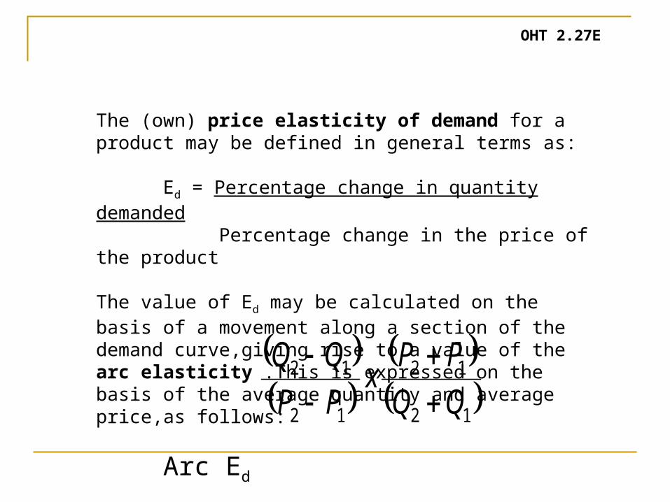
The (own) price elasticity of demand for a product may be defined in general terms as:
Ed = Percentage change in quantity demanded Percentage change in the price of the product
The value of Ed may be calculated on the basis of a movement along a section of the demand curve,giving rise to a value of the arc elasticity .This is expressed on the basis of the average quantity and average price,as follows:
Arc Ed
OHT 2.27E
12
12
12
12
PPx
PP
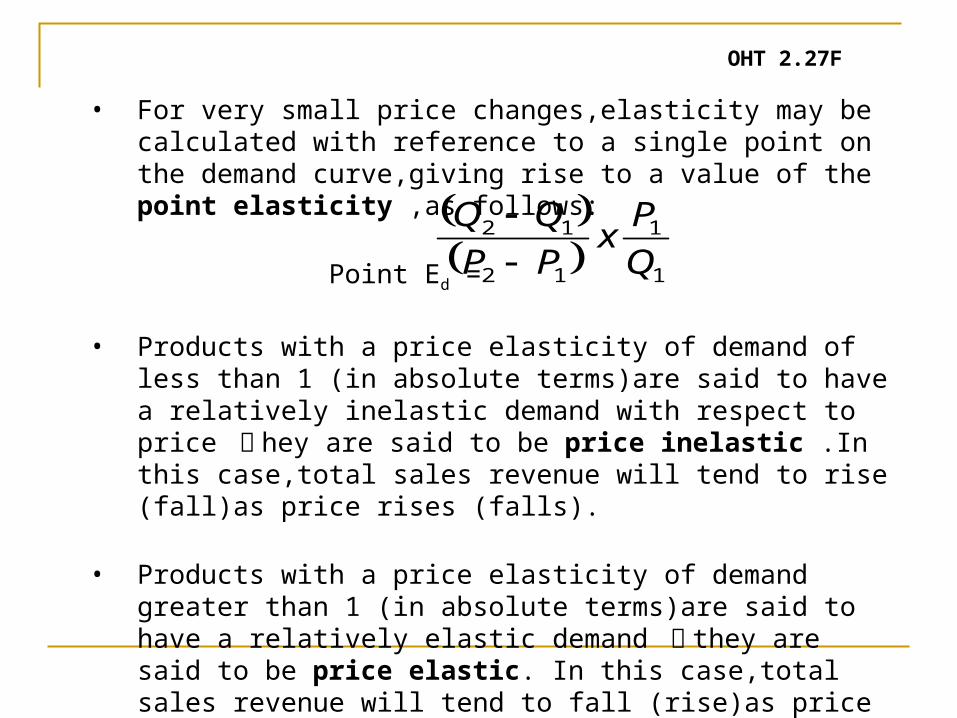
• For very small price changes,elasticity may be calculated with reference to a single point on the demand curve,giving rise to a value of the point elasticity ,as follows:
Point Ed =
• Products with a price elasticity of demand of less than 1 (in absolute terms)are said to have a relatively inelastic demand with respect to price 釦 hey are said to be price inelastic .In this case,total sales revenue will tend to rise (fall)as price rises (falls).
• Products with a price elasticity of demand greater than 1 (in absolute terms)are said to have a relatively elastic demand 釦they are said to be price elastic. In this case,total sales revenue will tend to fall (rise)as price rises (falls).
OHT 2.27F
1
1
12
12
Q
Px
PP
• Products with a price elasticity of demand equal to 1 (in absolute terms)are said to have a unit or unitary elasticity of demand. In this case, total sales revenue will remain unchanged as price rises or falls.
• The value of price elasticity of demand can range from infinity (in absolute terms)to 0. A product with a perfectly inelastic demand will have a value of Ed equal to 0 at every price,while a product with a perfectly elastic demand will have a value of Ed equal to infinity at a particular price.
• Cross-price elasticity of demand indicates the responsiveness of the demand for one product to changes in the prices of other goods and services and may be calculatedas:
Cross-price Ed = Percentage change in the demand for A Percentage change in the price of B
OHT 2.27G
• Substitutes will tend to have a positive value for cross-price Ed ,while complements will tend to have a negative value.
• Income elasticity of demand measures the responsiveness of quantity demanded with respect to (real) income variations as follows:
Income Ed = Percentage change in quantity demanded
Percentage change in real incomeNecessities exhibit a positive income elasticity of demand though the value will tend to be less than 1. In contrast, luxuries will tend to have an income elasticity of demand greater than 1.
• Marginal revenue is defined as the incremental change in total revenue and is usually measured as a firm sells one more or one less unit of its output.
OHT 2.27H
• The marginal revenue curve declines at twice the rate of the demand (average revenue)curve.
• When total revenue is increasing (decreasing),marginal revenue is positive (negative)such that total revenue is maximised when marginal revenue is zero .This occurs when the price elasticity of demand is equal to 1.
• An indifference curve shows all combinations of two goods or services that yield the same level of utility or satisfaction so that the consumer is indifferent between each combination.
• The slope of the budget line is determined by the relative prices of the two goods or services and the position of the line by the consumer 痴 income.
OHT 2.27I
• Together, the indifference curve mapping and the budget line determine the combination of the goods or services that the consumer will choose to buy.
• Indifference curve analysis can be used to show the income and substitution effects of a price change.
OHT 2.27J
OHT A2.28
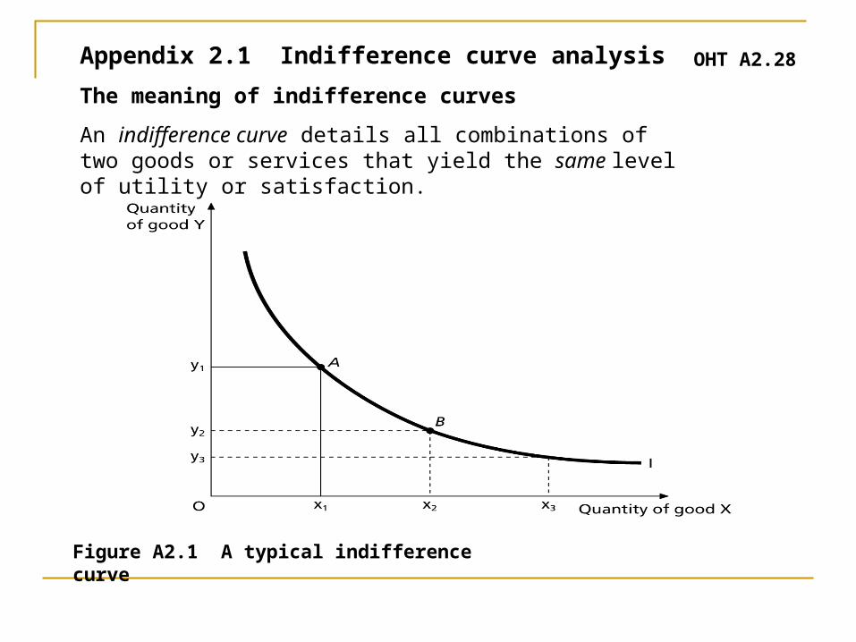
Figure A2.1 A typical indifference curve
Appendix 2.1 Indifference curve analysis
The meaning of indifference curves
An indifference curve details all combinations of two goods or services that yield the same level of utility or satisfaction.
OHT A2.29
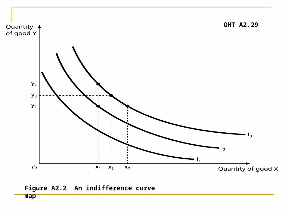
Figure A2.2 An indifference curve map
OHT A2.30
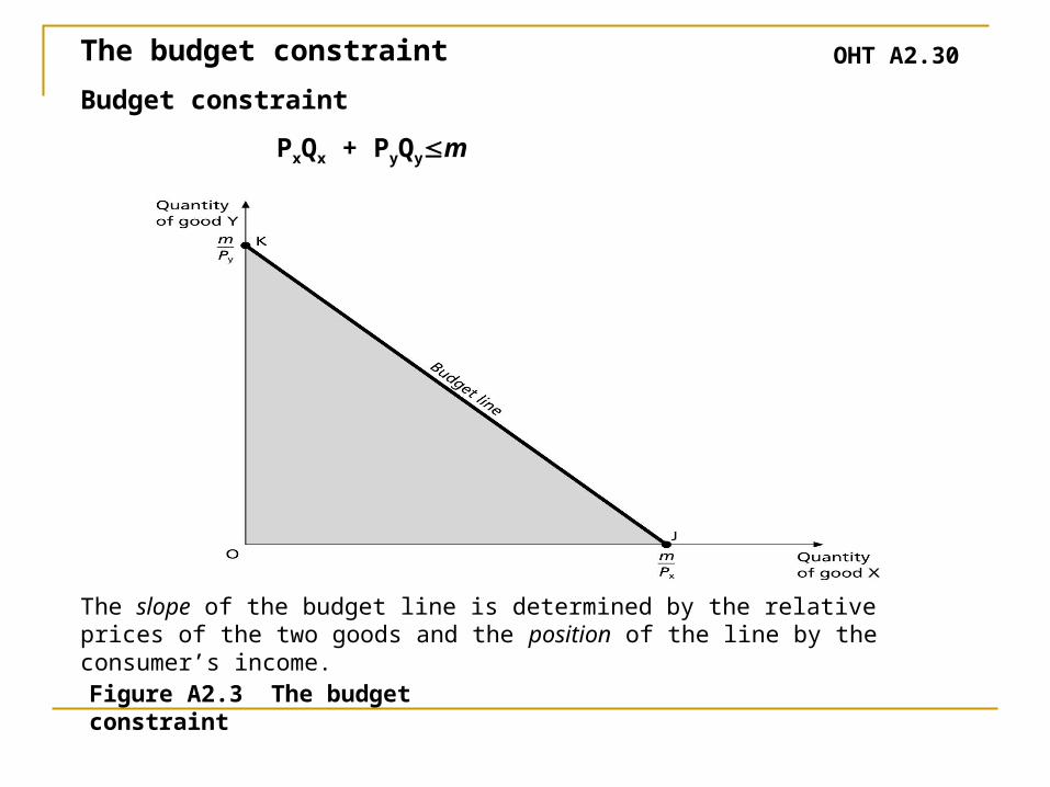
Figure A2.3 The budget constraint
The budget constraint
Budget constraint
PxQx + PyQym
The slope of the budget line is determined by the relative prices of the two goods and the position of the line by the consumer’s income.
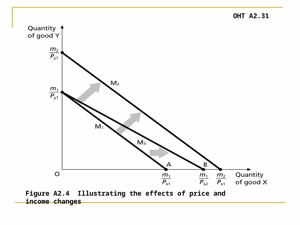
OHT A2.31
Figure A2.4 Illustrating the effects of price and income changes
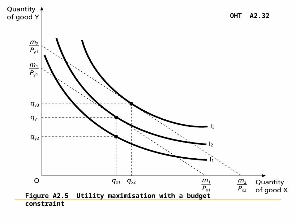
OHT A2.32
Figure A2.5 Utility maximisation with a budget constraint
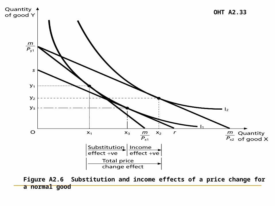
OHT A2.33
Figure A2.6 Substitution and income effects of a price change for a normal good
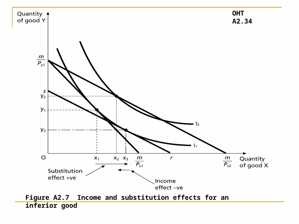
OHT A2.34
Figure A2.7 Income and substitution effects for an inferior good
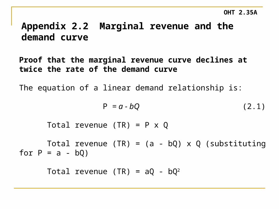
Proof that the marginal revenue curve declines at twice the rate of the demand curve
The equation of a linear demand relationship is:
P = a - bQ (2.1)
Total revenue (TR) = P x Q
Total revenue (TR) = (a - bQ) x Q (substituting for P = a - bQ)
Total revenue (TR) = aQ - bQ2
OHT 2.35A
Appendix 2.2 Marginal revenue and the demand curve
OHT 2.35B
Appendix 2.2 Marginal revenue and the demand curve
Q
bQaQ
2
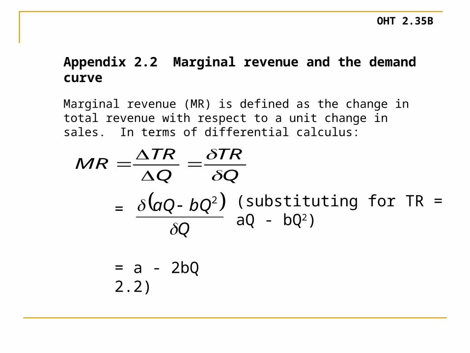
Marginal revenue (MR) is defined as the change in total revenue with respect to a unit change in sales. In terms of differential calculus:
Q
TR
Q
TRMR
= a - 2bQ2.2)
(substituting for TR = aQ - bQ2)=