Embed Size (px)
Citation preview

The Manga Guide™ to
Linear aLGebra
Shin Takahashi, iroha inoue, and
Trend-Pro Co., Ltd.
Supplemental appendixes
Copyright © 2012 by Shin Takahashi and TREND-PRO Co., Ltd.ISBN-13: 978-1-59327-413-9

ii Contents
Contents
a Workbook . . . . . . . . . . . . . . . . . . . . . . . . . . . . . . . . . . . . . . . . . . . . . . . . . . . . . 1
Problem Sets . . . . . . . . . . . . . . . . . . . . . . . . . . . . . . . . . . . . . . . . . . . . . . . . . . . . . 2Solutions . . . . . . . . . . . . . . . . . . . . . . . . . . . . . . . . . . . . . . . . . . . . . . . . . . . . . . . . 4
b Vector Spaces. . . . . . . . . . . . . . . . . . . . . . . . . . . . . . . . . . . . . . . . . . . . . . . . . 11
C Dot Product . . . . . . . . . . . . . . . . . . . . . . . . . . . . . . . . . . . . . . . . . . . . . . . . . . 15
Norm. . . . . . . . . . . . . . . . . . . . . . . . . . . . . . . . . . . . . . . . . . . . . . . . . . . . . . . . . . . 16Dot Product . . . . . . . . . . . . . . . . . . . . . . . . . . . . . . . . . . . . . . . . . . . . . . . . . . . . . 17The Angle Between Two Vectors . . . . . . . . . . . . . . . . . . . . . . . . . . . . . . . . . . . . . 18Inner Products . . . . . . . . . . . . . . . . . . . . . . . . . . . . . . . . . . . . . . . . . . . . . . . . . . . 19
Real Inner Product Spaces . . . . . . . . . . . . . . . . . . . . . . . . . . . . . . . . . . . . . . 19Orthonormal Bases . . . . . . . . . . . . . . . . . . . . . . . . . . . . . . . . . . . . . . . . . . . . . . . 20
D Cross Product . . . . . . . . . . . . . . . . . . . . . . . . . . . . . . . . . . . . . . . . . . . . . . . . 21
What Is the Cross Product?. . . . . . . . . . . . . . . . . . . . . . . . . . . . . . . . . . . . . . . . . 22Cross Product and Parallelograms . . . . . . . . . . . . . . . . . . . . . . . . . . . . . . . . . . . 23Cross Product and Dot Product. . . . . . . . . . . . . . . . . . . . . . . . . . . . . . . . . . . . . . 25
e Useful Properties of Determinants . . . . . . . . . . . . . . . . . . . . . . . . . . . . 27

AWorkbook

2 Appendix A
? Problem Sets
Problem Set 1
Let’s start off with the 2×2 matrix 45
−1−2
. Use it in the following six problems.
1. Calculate the determinant.
2. Use the formula =a11
a21
a12
a22
a22
−a21
−a12
a11
−11
a11 a22−a12 a21 to calculate the
inverse.
3. Find the inverse using Gaussian elimination.
4. Find all eigenvalues and eigenvectors.
5. Express the matrix in the form x11
x21
x12
x22
x11
x21
x12
x22
λ1
00λ2
−1
6. Solve the linear system of equations 4x1−1x2 = 1
5x1−2x2 = −1 using Cramer’s rule.
Problem set 2
Next up is the 3×3 matrix
1
2
3
4
1
−2
−1
2
−1. Use it in the following two problems.
1. Prove that the matrix column vectors
1
2
3,
4
1
−2, and
−1
2
−1 are linearly
independent (i.e., that the matrix rank is equal to three).
2. Calculate the determinant.

Workbook 3
Problem set 3
Determine whether the following sets are subspaces of R3.
1. α and β are arbitrary real numbers
αβ
5α−7β
2. αβ
5α−7
α and β are arbitrary real numbers
note Have a look at Appendixes C and D before trying problem set 4.
Problem Set 4
Let’s deal with the vectors
1
2
3 and
4
1
−2 for the next set of problems.
1. Calculate the distance to the origin for both vectors.
2. Calculate the scalar product of the two vectors.
3. Calculate the angle between the two vectors.
4. Calculate the cross product of the two vectors.

4 appendix a
! Solutions
Problem Set 1
1. 4
5
−1
−2= 4 · (−2) − (−1) · 5 = −8 + 5 = −3det
2. 1
4 · (−2) − (−1) · 5
1
−3
1
4
−2
−5
1
4
−2
−5=
1
3=
2
5
−1
−4
3. Here is the solution:
4
5
−1
−2
1
0
0
1
3
5
0
−2
2
0
−1
1
15
0
0
−6
10
−10
−5
8
Multiply row 1 by 2 and subtract row 2 from row 1.
Multiply row 1 by 5 and row 2 by 3. Subtract row 1 from row 2.
Divide row 1 by 15 and row 2 by −6.
0
1
1
0
1
3−
4
3−
2
3
5
3
4. The eigenvalues are roots of the characteristic equation
4 − λ5
−1
−2 − λ det = 0

Workbook 5
and are as follows:
4 − λ5
−1
−2 − λ= (4 − λ) · (−2 − λ) − (−1) · 5
= (λ − 4)(λ + 2) + 5
= λ2 − 2λ − 3
= (λ − 3)(λ + 1) = 0
det
λ = 3, −1
a. Eigenvectors corresponding to λ = 3
Plugging our value into x1
x2
x1
x2
= λ4
5
−1
−2,
that is 0
0
x1
x2
=4 − λ
5
−1
−2 − λ ,
gives us 1
5
−1
−5
1
5
0
0
4 − 3
5
−1
−2 − 3
x1
x2
x1
x2
x1
5x1
−x2
−5x2
= = == [x1 − x2] .
We see that x1 = x2, which leads us to the eigenvector
x1
x2
c1
c1
1
1= = c1
where c1 is a real nonzero number.
b. Eigenvectors corresponding to λ = −1
Plugging −1 into the matrix gives us this:
5
5
−1
−1
1
1
0
0
4 − (−1)
5
−1
−2 − (−1)
x1
x2
x1
x2
5x1
5x1
−x2
−x2
= = == [5x1 − x2]
We see that 5x1 = x2, which leads us to the eigenvector
x1
x2
c2
5c2
1
5= = c2
where c2 is a real nonzero number.
6 Appendix A
5. From problem 4:
=4
5
−1
−2
3
0
0
−1
1
1
1
5
1
1
1
5
−1
6. The linear system of equations 4x1 − 1x2 = 1
5x1 − 2x2 = −1 can be rewritten as follows:
=1
−1
x1
x2
4
5
−1
−2
Using the methods from problem 1, we are easily able to infer the roots using Cramer’s rule.
• x1 = = = = 1 4
5
−1
−2det
1
−1
−1
−2det
1 · (−2) − (−1) · (−1)
−3
−3
−3
• x2 = = = = 3 4
5
−1
−2det
4
5
1
−1det
4 · (−1) − 1 · 5
−3
−9
−3

Workbook 7
Problem Set 2
1. It looks like the rank of the matrix
1
2
3
4
1
−2
−1
2
−1
is 3 from inspection, but let’s use the following table, just to be sure.
Add (−2 times row 1) to row 2 and (−3 times row 1) to row 3.
Add (−2 times row 2) to row 3.
1
−2
−3
0
1
0
0
0
1
1
2
3
4
1
−2
−1
2
−1
1
0
0
4
−7
−14
−1
4
2
=
Add ( times row 3) to row 1 and ( times row 3) to row 2.1
6−
4
6
1
0
0
0
1
−2
0
0
1
1
0
0
4
−7
0
−1
4
−6
1
0
0
4
−7
−14
−1
4
2
=
Add ( times row 2) to row 1.
1
0
0
4
−7
0
−1
4
−6
1
0
0
4
−7
0
0
0
−6
=
0
1
0
1
0
0
1
6−
4
6
1
1
2
3
4
1
−2
−1
2
−1
4
7
1
0
0
4
−7
0
0
0
−6
1
0
0
0
−7
0
0
0
−6
=
471
0
0
0
0
1
1
0

8 appendix a
The two matrices
1
2
3
4
1
−2
−1
2
−1
and
1
0
0
0
−7
0
0
0
−6
have the same rank, as
we saw on pages 196–201.
Since the number of linearly independent vectors among
1
0
0
,
0
−7
0
, and
0
0
−6
is obviously 3,
the rank of both
1
2
3
4
1
−2
−1
2
−1
and
1
0
0
0
−7
0
0
0
−6
also must be 3.
Note that the solution is apparent in step three of the table, since triangu-lar n×n matrices with nonzero main diagonal entries have rank n. This is also true for nonsquare matrices.
2.
= 1 · 1 · (−1) + 4 · 2 · 3 + (−1) · 2 · (−2) − (−1) · 1 · 3 − 4 · 2 · (−1) − 1 · 2 · (−2)
= −1 + 24 + 4 + 3 + 8 + 4 = 42
det
1
2
3
4
1
−2
−1
2
−1

Workbook 9
Problem Set 3
Suppose c is an arbitrary real number.
1. The set is a subspace since both conditions are met.
αβ
5α − 7β
α1
β1
5α1 − 7β1
α2
β2
5α2 − 7β2
α1 + α2
β1 + β2
5(α1 + α2) − 7(β1 + β2)
+ = ∈α and β are arbitrary real numbers
αβ
5α − 7β
α1
β1
5α1 − 7β1
c
cα1
cβ1
5(cα1) − 7(cβ1)
= ∈α and β are arbitrary real numbers
2. The set is not a subspace since neither condition is met.1
αβ
5α − 7
α1
β1
5α1 − 72
2α1
2β1
5(2α1) − 14
2α1
2β1
5(2α1) − 7= ≠ ∈
α1
β1
5α1 − 7
α2
β2
5α2 − 7+
≠
αβ
5α−7
α1 + α2
β1 + β2
5(α1 + α2) − 14
α1 + α2
β1 + β2
5(α1 + α2) − 7= ∈
α and β are
arbitrary
real numbers
α and β are
arbitrary
real numbers
1. Both conditions on page 151 have to be met for the subset to be a subspace. This means that checking the second condition is unnecessary if we find that the first condition doesn’t hold.

10 appendix a
Problem Set 4
1.
1
2
3
= 12 + 22 + 32 = =1 + 4 + 9 14
4
1
−2
= 42 + 12 + (−2)2 = =16 + 1 + 4 21
2. · = 1 · 4 + 2 · 1 + 3 · (−2) = 4 + 2 − 6 = 0
1
2
3
4
1
−2
3. The angle between
1
2
3
and
4
1
−2
can be calculated using the dot product for-mula as follows:
cos θ = = = 0
·
1
2
3
4
1
−2
1
2
3
4
1
−2
·
14 21·
0
So the angle is cos−1 0 = 90 degrees.
4.
1
2
3
2 · (−2)
3 · 4
1 · 1
4
1
−2
−1
2
−1
−7
14
−7
(−4) − 3
12 + 2
1 − 8
= = = = 7×
−
−
−
1 · 3
(−2) · 1
4 · 2

BVector Spaces

12 appendix b
On page 16 (Chapter 1) it was mentioned that linear algebra is generally about translating something residing in an m-dimensional space into a corresponding shape in an n-dimensional space. This is by all means true, though understand-ing a more general interpretation of linear algebra might give you an edge if you decide to study the subject further.
In this interpretation, most of the interesting calculations and theorems have to do with something called vector spaces, which are described on the next page. Note that there is a difference between these vectors and the ones presented in Chapter 4—the ones we’re discussing here are a much more abstract concept.
The basic idea is this: Much as you play football on football fields and golf on golf courses, you calculate linear algebra in vector spaces.
But before we get into the technical definition of a vector space, let’s look at a couple of simple, concrete examples.
example 1
The first example may already be familiar: Let’s say that X is the set of all ordered triples of real numbers. So two of the many elements in X are (1.0, 2.3, −4.6) and (0.0, −5.7, 8.1). This infinite set of ordered triples forms a vector space (as described by the axioms listed on the next page). X is a vector space, and (1.0, 2.3, −4.6) is a vector.
example 2
As a second example, consider these two polynomials with real coefficients:
7t4 − 3t − 4 and 2t − 1
These polynomials could be considered vectors, if we view the set of all poly-nomials up to the fourth degree as a vector space.

Vector Spaces 13
The eight axioms of Vector Spaces
Assume that x, y, and z are elements of the set X, and that c and d are two arbitrary numbers.
If X satisfies the following two sets of axioms, we say that X is a vector space and x, y, and z are vectors.
addition axioms:The set has to be closed under vector addition. This means that the sum of two elements of the set also belongs to the set.
Vector addition must also satisfy the following four conditions:
1. (x + y) + z = x + (y + z) (associativity)
2. x + y = y + x (commutativity)
3. A zero vector (0) exists with the following properties: x + 0 = 0 + x = x
4. An inverse vector (−x) exists with the following properties: x + (−x) = (−x) + x = 0
Scalar Multiplication axioms:The set has to be closed under scalar multiplication. This means that the product of an element of the set and an arbitrary number also belongs to the set.
Scalar multiplication must also satisfy the following four conditions:
5. c(x + y) = cx + cy
6. (cd)x = c(dx)
7. (c + d)x = cx + dx
8. 1x = x
In this book we always assume that scalar multiplication is done with real numbers. Such vector spaces are usually called real vector spaces. Vector spaces also allowing multiplication with complex numbers would similarly be called complex vector spaces.


CDot Product

16 appendix C
norm
Suppose we have an arbitrary vector in Rn
x1
x2
xn
.
The vector norm or length is then equal to x1
2 + x22 + ... + xn
2
and is written
x1
x2
xn
.
example 1
1
3= 12 + ( 3 )2 = =1 + 3 4 = 2
2 − 6
2 + 6= ( 2 − 6)2 + ( 2 + 6)2 = 16 = 4= 2 − 2 12 + 6 + 2 + 2 12 + 6
example 2
1
3= 12 + ( 3 )2 = =1 + 3 4 = 2
2 − 6
2 + 6= ( 2 − 6)2 + ( 2 + 6)2 = 16 = 4= 2 − 2 12 + 6 + 2 + 2 12 + 6

Dot Product 17
Dot Product
Suppose we have two arbitrary vectors
x1
x2
xn
and
y1
y2
yn
in Rn.
The vector’s dot product1 is defined as follows:
x1y1 + x2 y2 + ... + xn yn
This is usually represented with a dot ( ∙ ) like so:
x1
x2
xn
x1
x2
xn
·
example
1
3
2 − 6
2 + 6· = 1 · ( 2 − 6) + 3 · ( 2 + 6) = 2 − 6 + 6 + 18 = 2 + 3 2 = 4 2
1. The dot product is sometimes referred to as the scalar product.
18 appendix C
The angle between Two Vectors
Suppose we have two arbitrary vectors
x1
x2
xn
and
y1
y2
yn
in Rn.
The angle θ between those two vectors can be found using the following relationship:
x1
x2
xn
y1
y2
yn
· =
x1
x2
xn
y1
y2
yn
· · cos θ
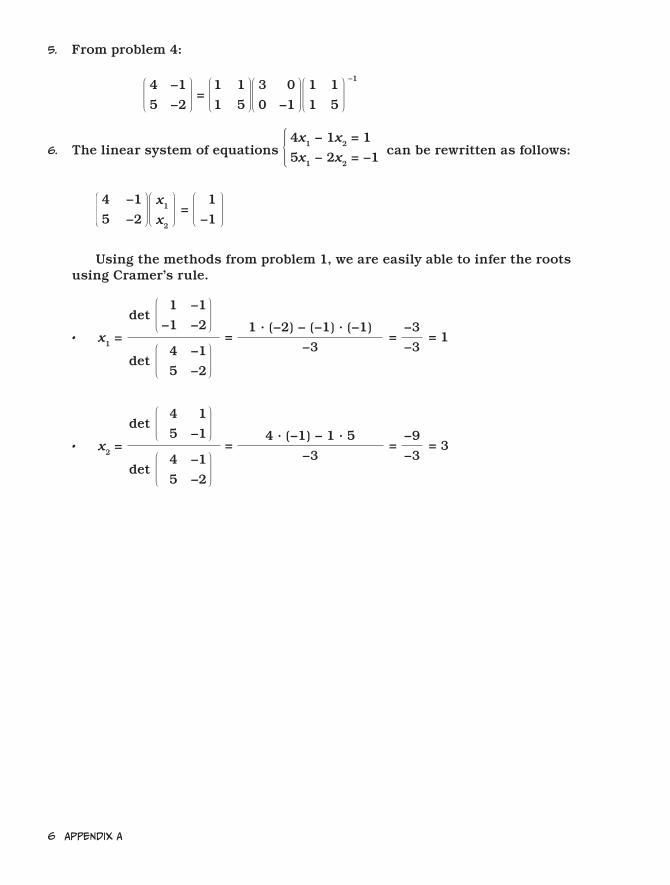
example
The angle θ between the two vectors 1
3 and 2 − 6
2 + 6 can be found using the formula:
1
3
2 − 6
2 + 6·
2 − 6
2 + 6
1
3·
cos θ = =4 2
2 · 4 2
2=
So θ = 45 degrees.
2 − 6
2 + 6
3
θ
O 1

Dot Product 19
inner Products
The dot product is actually a special case of a more general concept that has some very interesting applications. That general concept is a function, called an inner product, that maps two vectors to a real number and also satisfies some special properties. There are also inner product spaces,2 which are vector spaces that have an associated inner product, as described below.
real inner Product Spaces
We say that the real vector space X is a real inner product space or Euclidean space if there exists a real inner product <x, y> which maps a pair of vectors to a scalar and satisfies the following conditions for all vectors x, y, z, and all scalars c:
<x, y> = <y, x>
<cx, y> = c<x, y> = <x, cy>
<x, y + z> = <x, y> + <x, z> and <x + y, z> = <x, z> + <y, z>
<x, x> ≥ 0 and <x, x> = 0 only when x = 0 (the zero vector).
The dot product is the most familiar example of an inner product. In that example, we define
<x, y> = x1y1 + x2y2 + ... + xnyn
2. The subject is outside the scope of this book, but inner products also appear in complex product spaces.

20 appendix C
Orthonormal bases
Vector sets like
1
0
0
1,
1
2
1
1,
1
2
−1
1 and
1
2
3
4
1
−2
−1
2
−1
1
14
1
21
1
6, ,
where
• the norm of every vector is equal to 1
• the dot product of each vector pair is equal to 0
are called orthonormal bases or ON-bases.The Gram-Schmidt orthogonalization process can be used to create an ortho-
normal basis from any arbitrary basis, but it is outside the scope of this book.

DCross Product

22 appendix D
What is the Cross Product?
Suppose we have two arbitrary vectors
a
b
c
and
P
Q
R
in R3.
The vector cross product is defined as
bR − Qc
cP − Ra
aQ − Pb
and is usually represented with a cross like so:
P
Q
R
a
b
c
note The cross product is defined only in R3. In contrast, the dot product is
defined in Rn for all positive n.
Here’s a good mnemonic for remembering the combinations in calculating the cross product of two vectors:
P
Q
R
a
b
c
P
Q
R
a
b
c
Start by writing the elements of each vector twice, as you can see above. Ignoring the first and last rows, draw an arrow from each element to the one below it in the opposite vector.
Arrows going from left to right get a plus sign; arrows going from right to left get a minus sign. The top pair of arrows produces the first component of the cross product, the middle pair produces the second component, and the bottom pair produces the last component.
Cross Product 23
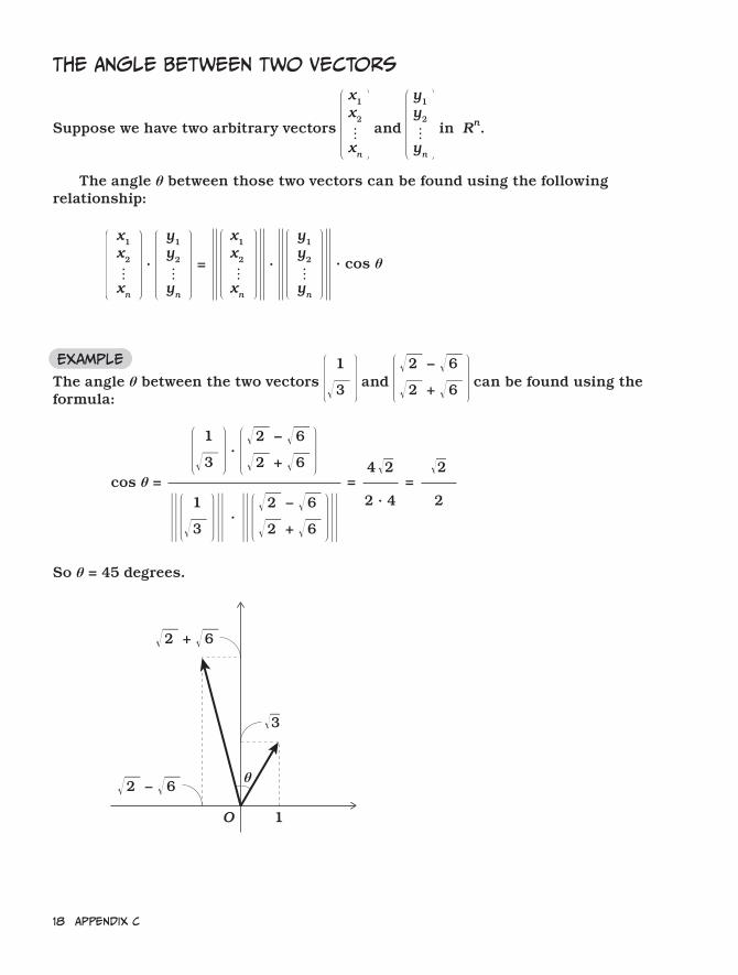
Cross Product and Parallelograms
Consider the following cross product:
P
Q
R
a
b
c
u It is perpendicular to both vectors
P
Q
R
and
a
b
c
.
v Its length is equal to the area of the parallelogram with sides
P
Q
R
and
a
b
c
.
Both properties are illustrated in the picture below.
a
b
c
P
Q
R
O
P
Q
R
a
b
c
note This picture is using a “right handed” coordinate system. That means that
your right thumb will point in the direction of the cross product if you do the fol-
lowing: Stick your thumb out so it is perpendicular to your lower arm, then use
your remaining four fingers to form the letter C. Starting with the base of your
fingers as the vector on the left side of the cross product, orient your hand so
the tips of your fingers are pointing toward the vector on the right side of the
cross product. Your thumb will then be pointing in the direction of the result of
the cross product! Note that if you switch the positions of the vectors, the cross
product will reverse direction.
24 appendix D
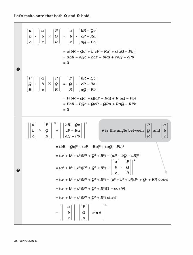
Let’s make sure that both and hold.
a
b
c
a
b
c
P
Q
R
a
b
c
bR − Qc
cP − Ra
aQ − Pb =· ·
= a(bR − Qc) + b(cP − Ra) + c(aQ − Pb)
= abR − aQc + bcP − bRa + caQ − cPb
= 0
a
b
c
P
Q
R
bR − Qc
cP − Ra
aQ − Pb =· ·
P
Q
R
P
Q
R
= P(bR − Qc) + Q(cP − Ra) + R(aQ − Pb)
= PbR − PQc + QcP − QRa + RaQ − RPb
= 0
a
b
c
P
Q
R
2
=
bR − Qc
cP − Ra
aQ − Pb
2
= (bR − Qc)2 + (cP − Ra)2 + (aQ − Pb)2
= (a2 + b2 + c2)(P2 + Q2 + R2) −
a
b
c
P
Q
R
·
2
= (a2 + b2 + c2)(P2 + Q2 + R2) − (a2 + b2 + c2)(P2 + Q2 + R2) cos2θ
= (a2 + b2 + c2)(P2 + Q2 + R2)(1 − cos2θ)
= (a2 + b2 + c2)(P2 + Q2 + R2) sin2θ
= (a2 + b2 + c2)(P2 + Q2 + R2) − (aP + bQ + cR)2
a
b
c
P
Q
Rsin θ
2
=
θ is the angle between and
P
Q
R
a
b
c

Cross Product 25
Cross Product and Dot Product
The table below contains a comparison between cross and dot products.
Cro� Product Dot Product
1
2
3
4
5
6
=
2 · 6 − 5 · 3
3 · 4 − 6 · 1
1 · 5 − 4 · 2
= −
5 · 3 − 2 · 6
6 · 1 − 3 · 4
4 · 2 − 1 · 5
= −
4
5
6
1
2
3
1
2
3
4
5
6
· = 1 · 4 + 2 · 5 + 3 · 6
= 4 · 1 + 5 · 2 + 6 · 3 =
1
2
3
4
5
6
·
1c
2c
3c
4
5
6
=
2c · 6 − 5 · 3c
3c · 4 − 6 · 1c
1c · 5 − 4 · 2c
= c
2 · 6 − 5 · 3
3 · 4 − 6 · 1
1 · 5 − 4 · 2
= c
1
2
3
4
5
6
1c
2c
3c
4
5
6
· = 1c · 4 + 2c · 5 + 3c · 6
= c (1 · 4 + 2 · 5 + 3 · 6) = c
1
2
3
4
5
6
·
1
2
3
4
5
6
7
8
9
+
=
1
2
3
4 + 7
5 + 8
6 + 9
=
2 · (6 + 9) − (5 + 8) · 3
3 · (4 + 7) − (6 + 9) · 1
1 · (5 + 8) − (4 + 7) · 2
=
2 · 6 − 5 · 3
3 · 4 − 6 · 1
1 · 5 − 4 · 2
+
2 · 9 − 8 · 3
3 · 7 − 9 · 1
1 · 8 − 7 · 2
= +
1
2
3
4
5
6
1
2
3
7
8
9
1
2
3
4
5
6
7
8
9
+
=
1
2
3
4 + 7
5 + 8
6 + 9
·
·
= 1 · (4 + 7) + 2 · (5 + 8) + 3 · (6 + 9)
= (1 · 4 + 2 · 5 + 3 · 6) + (1 · 7 + 2 · 8 + 3 · 9)
= +
1
2
3
4
5
6
1
2
3
7
8
9
· ·


EUseful Properties of
Determinants

28 appendix e
Determinants have several interesting properties. We’ll look at seven of them in this appendix.
Property 1
For any square matrix A, det A = det AT.
a11
an1
a1n
ann
a11
an1
a1n
ann
det = det
T
example
• 3
0
0
2det = 6
O
2
3
• 3
0
0
2det = 6
3
0
0
2= det
T
O
2
3

Useful Properties of Determinants 29
Property 2
If two columns or two rows of A are interchanged, resulting in matrix B, then det B = −det A.
a11
an1
a1i
ani
det = (−1)det
a1j
anj
a1n
ann
a11
an1
a1n
ann
a1i
ani
a1j
anj
example
• 3
0
0
2det = 6
O
2
3
• (−1)det = (−1) · (−6) = 63
0
0
2
O
2
3

30 appendix e
Property 3
If A has two identical columns or two identical rows, then det A = 0.
a11
an1
b1
bn
det = 0
b1
bn
a1n
ann
column i column j
example
• 3
0
3
0det = 0
O 3
The area is equal to zero.

Useful Properties of Determinants 31
Property 4
If a column or row of A is multiplied by the constant c, resulting in matrix B, then det B = c det A, or equivalently, det A = ¹⁄c det B.
a11
an1
a1i · c
ani · cdet = c det
a1n
ann
a11
an1
a1n
ann
a1i
ani
example
• 3
0
0
2det = 6
O
2
3
• 3 · 2
0 · 2
0
2det = det
6
0
0
2= 2 · 6 = 2 det
3
0
0
2
O
2
6
32 appendix e
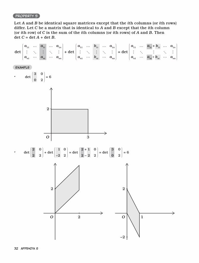
Property 5
Let A and B be identical square matrices except that the ith columns (or ith rows) differ. Let C be a matrix that is identical to A and B except that the ith column (or ith row) of C is the sum of the ith columns (or ith rows) of A and B. Then det C = det A + det B.
det
a11
an1
a1n
ann
a1i
ani
+ det
a11
an1
a1n
ann
b1i
bni
= det
a11
an1
a1i + b1i
ani + bni
a1n
ann
example
• 3
0
0
2det = 6
O
2
3
• det 2
2
0
2+ det
1
−2
0
2
2 + 1
2 − 2
0
2= det
3
0
0
2= det = 6
O
2
2 O
2
1
−2

Useful Properties of Determinants 33
Property 6
Let B be the matrix formed by replacing column j (or row j) of A with the sum of column j (or row j) of A and a nonzero multiple, c, of column i (or row i) of A, where i ≠ j. Then det B = det A.
det = det
a11
an1
a1i
ani
a1j
anj
a1n
ann
a11
an1
a1i
ani
a1j + (a1i · c)
anj + (ani · c)
a1n
ann
example
• 3
0
0
2det = 6
O
2
3
• 3
0
3
2= 6
3
0
0 + (3 · 1)
2 + (0 · 1)det = det
O
2
3 6

34 appendix e
Property 7
Let A and B be any two square matrices. Then (det A)(det B) = det (AB).
a11
an1
a1n
ann
b11
bn1
b1n
bnn
det det
a11
an1
a1n
ann
b11
bn1
b1n
bnn
= det
example
• 3
0
0
2det · det
0
013
12
= 6 ·16
= 1
O
2
3 13
12
O
• 3
0
0
2det
0
013
12
= det1
0
0
1= 1
O
1
1