Space Sci RevDOI 10.1007/s11214-010-9667-6

The Magnetic Field of the Earth’s Lithosphere

Erwan Thébault · Michael Purucker · KathrynA. Whaler · Benoit Langlais · Terence J. Sabaka

Received: 23 December 2009 / Accepted: 17 June 2010© Springer Science+Business Media B.V. 2010

Abstract The lithospheric contribution to the Earth’s magnetic field is concealed in mag-netic field data that have now been measured over several decades from ground to satellitealtitudes. The lithospheric field results from the superposition of induced and remanent mag-netisations. It therefore brings an essential constraint on the magnetic properties of rocks ofthe Earth’s sub-surface that would otherwise be difficult to characterize. Measuring, extract-ing, interpreting and even defining the magnetic field of the Earth’s lithosphere is howeverchallenging. In this paper, we review the difficulties encountered. We briefly summarizethe various contributions to the Earth’s magnetic field that hamper the correct identificationof the lithospheric component. Such difficulties could be partially alleviated with the jointanalysis of multi-level magnetic field observations, even though one cannot avoid makingcompromises in building models and maps of the magnetic field of the Earth’s lithosphere

E. Thébault (�)Institut de Physique du Globe de Paris, Equipe de Géomagnétisme, CNRS UMR7154, 4, place Jussieu,75252 Paris, Francee-mail: ethebault@ipgp.jussieu.fr

M. PuruckerRaytheon at Planetary Geodynamics Lab, Code 698, NASA/Goddard Space Flight Center, Greenbelt,MD 20771, USAe-mail: michael.e.purucker@nasa.gov

K.A. WhalerSchool of GeoSciences, University of Edinburgh, Edinburgh, UKe-mail: kathy.whaler@ed.ac.uk

B. LanglaisLaboratoire de Planétologie et Géodynamique, CNRS UMR 6112 and Université de Nantes,2 rue de la Houssinière, 44000 Nantes, Francee-mail: benoit.langlais@univ-nantes.fr

T.J. SabakaPlanetary Geodynamics Branch, Code 698, NASA/Goddard Space Flight Center, Greenbelt, MD 20771,USAe-mail: Terence.J.Sabaka@nasa.gov

E. Thébault et al.

at various altitudes. Keeping in mind these compromises is crucial when lithospheric fieldmodels are interpreted and correlated with other geophysical information. We illustrate thisdiscussion with recent advances and results that were exploited to infer statistical propertiesof the Earth’s lithosphere. The lessons learned in measuring and processing Earth’s mag-netic field data may prove fruitful in planetary exploration, where magnetism is one of thefew remotely accessible internal properties.

Keywords Lithospheric magnetic field · Modelling · Regional modelling · Planetarymagnetic field · Satellite

1 Introduction

The Earth’s magnetic field results from the superposition of fields of various origins thatoperate on a wide range of spatial and temporal scales. On the Earth, the magnetic field isubiquitous and it is no surprise that this physical quantity has been continuously measuredfor more than a century (Mandea and Purucker 2005). Geomagnetic field measurements areof widespread use for remote sensing, natural resource exploration, geophysical research,planetary science, and societal applications (Kono 2007). In particular, their interpretationwas crucial to the development of a new paradigm of geosciences in the early 1960, that ofPlate Tectonics (Vine and Matthew 1963).

The large amount of available data from ground to satellite altitudes paradoxically leadsto difficulties, as surveys planned for identifying one type of magnetic field source are usu-ally not optimized for describing other source types.

This paper reviews the issues with which scientists have to deal when trying to extractthe magnetic contributions of the Earth’s lithosphere from a set of raw magnetic data. Wefocus on the most recent studies but the reader is referred to the book of Langel and Hinze(1998) that extensively reviewed the pioneering work carried out with satellite data prior tothe current epoch now commonly named the decade of geopotential field research (1999–2009).

In the first section, we recap some definitions widely used in geomagnetism and sum-marize the main properties of the Earth’s magnetic field sources. The main characteristic ofthe lithospheric field is that it is weak and overlapped by other sources in the magnetic fieldmeasurements. Hence, its complete description requires a large amount of spatially densemeasurements covering the Earth’s surface and various altitudes. We then briefly describethe available datasets that yield different lithospheric field maps and models and comparethe approaches. We finally focus on more geophysical interpretation and list some of theambiguities arising when interpreting the magnetic field and causative magnetisation of thelithosphere.

2 Generalities

2.1 Definitions

Away from magnetic sources, it was established by Gauss (1839) that the magnetic potentialobeys Laplace’s equation. The Earth’s magnetic field is derived from the magnetic potentialV and is expressed in nanotesla [nT]. In the geocentric reference frame, it can be expressedas

B = −∇V (r, θ,ϕ, t) (1)

The Magnetic Field of the Earth’s Lithosphere

with V being decomposed into Spherical Harmonics (SH)

V (r, θ,ϕ, t) = a

∞∑

n=1

n∑

m=0

(a

r

)n+1

(gmn (t) cos(mϕ) + hm

n (t) sin(mϕ))P mn (cos θ)

+ a

∞∑

n=1

n∑

m=0

(r

a

)n

(qmn (t) cos(mϕ) + sm

n (t) sin(mϕ))P mn (cos θ). (2)

The parameters a, r, θ , and φ are the Earth’s reference radius (6371.2 km), the radius, thegeocentric co-latitude, and the longitude respectively. (gm

n (t), hmn (t)) and (qm

n (t), smn (t)) are

the time-varying Gauss coefficients (in [nT]) of internal and external origin, respectively,with respect to the shell of radius r = a. In geomagnetism, P m

n (cos θ) is the Schmidt semi-normalized associated Legendre function of integer degree n and order m.

Lowes (1974) introduced the concept of the spatial power spectrum by the series

Rn = (n + 1)

(a

r

)2n+4 n∑

m=0

[(gm

n

)2 + (hm

n

)2]. (3)

Rn, expressed in nT2, gives an estimate of the contribution of each SH degree n to thesquared amplitude of the observed magnetic field of internal origin. We further introducethe definition of horizontal spatial wavelength λ in kilometres [km] associated with eachdegree n, following Backus et al. (1996, p. 101)

λ = 2πr√n(n + 1)

≈ 2πr

n(4)

for large n. Equations (3) and (4) show the dependency of the horizontal spatial resolutionwith the altitude of observation r . An important property is that small-scales are stronglyattenuated with upward continuation (increasing radius r), while they are enhanced withdownward continuation (decreasing radius r). In the following, the numerical values of thehorizontal wavelengths are given with respect to the Earth’s mean radius r = a.

2.2 The Masking Magnetic Field Sources

The magnetic field of the Earth’s lithosphere is not dominant but masked in the raw magneticdata by two major magnetic field sources that need to be briefly described. The reader isreferred to Hulot et al. (2007) for a general review of the different sources identified so farin magnetic field measurements.

From space, at radius r = a +h (where h is the altitude of the satellite), the geomagneticfield of internal origin is global in scale and dominantly dipolar. This contribution is oftenreferred to as the main field. At the Earth’s surface, this main field, mostly originating fromself-sustaining dynamo action in the liquid outer core, typically represents more than 98%of the total magnetic field and has a typical strength ranging from 20,000 nT at the equatorto 70,000 nT at the poles. The Earth’s core field is generated by currents flowing in theEarth’s liquid outer core between 2900 and 5200 km depth (note that a small percentage ofthis large-scale field is in fact induced by magnetic fields external to the Earth). This flowis responsible for a slow secular variation of the internal magnetic field (about 40 nT/yr onaverage) even though occasional abrupt changes of acceleration, referred to as geomagneticjerks, may occur (Courtillot et al. 1978; Chulliat et al. 2010). Over geological times, the main

E. Thébault et al.

field frequently reverses its polarity (Laj and Channel 2007). Many of these reversals areimprinted in the Earth’s crust giving a way to decipher at the same time the past behaviourof the Earth’s core magnetic field and the drift of Earth’s continents.

The second important sources for our discussion have strengths on average 3 to 4 ordersof magnitude lower than the main internal field (during quiet conditions). They are referredto as external fields and their sources lie in the ionosphere (for h = 100–150 km) and themagnetosphere (at distances of several Earth’s radii).

The ionospheric magnetic field is large-scale on average. The solar-quiet (Sq) magneticfield variations occur mainly in the dayside at middle and low latitudes. They are a mani-festation of two current vortices, one in each hemisphere, generated by tidal winds resultingfrom solar heating. This quasi-symmetric system is completed with an eastward-flowing cur-rent at the magnetic equator, called the equatorial electrojet (EEJ). This solar-mediated ter-restrial current system produces a magnetic field of a few tens of nT at low and mid-latitudes(depending on the local time and solar activity) on average but the magnetic signature of theEEJ can be locally much stronger.

The magnetospheric field is also a large-scale external field created by the coupling be-tween the Earth’s internal magnetic field, the solar wind plasma, and the interplanetary mag-netic field. It comes from a ring of current circulating roughly in the Earth’s magnetic equa-torial plane at a distance of several Earth radii (Baumjohann and Nakamura 2007) and has atypical magnitude of a few tens of nT at the Earth’s surface during quiet conditions.

The magnetospheric and ionospheric fields both result from sun-Earth interaction. Theirtime variations range between seconds and decades, with daily, seasonal, semi-annual andannual periodicities. Other variations are quasi-periodic and follow the solar cycle of 11 yrand 22 yr. At high latitude, especially during magnetically disturbed times, ionospheric andmagnetospheric fields are coupled via Field Aligned Currents (FAC). These create intensefields reaching several hundred nT in strength and having rapid time variations that are dif-ficult to monitor and thus to predict. Such a wide range of external magnetic field variabilityin space and time is particularly detrimental to lithospheric field studies.

3 The Lithospheric Field

3.1 The Sources of the Lithospheric Field

The magnetisation carried by rocks in the crust and upper mantle produces the lithosphericmagnetic field. The subject of rock magnetism is of considerable complexity but the mecha-nisms are well known in principle (see Dunlop and Özdemir 2007 for a recent review). Theamount of magnetisation depends on various parameters, such as the strength and directionof the ambient magnetic field, the mineralogy of the rock sample, its magnetic phase anddomain (if it is single or multi-domain and how easily the domain walls move under theinfluence of an ambient magnetic field), its grain size and shape, the amount of chemicalalteration, and the temperature. Most magnetic minerals on Earth are titano-magnetite andtitano-hematite for which the Curie temperatures are 580°C and 670°C respectively for thepure iron phases. On Earth, such temperatures are met at depths of typically 30 km in stablecontinental regions and 6–7 km in the oceanic regions. Deeper (and hotter) rocks are gen-erally considered nonmagnetic even though the Curie depth (i.e. the magnetic boundary),varying from place to place, is poorly known in detail.

The minerals found in the Earth’s crust are capable of carrying both remanent and in-duced magnetisations. Induced magnetisation arises when magnetic minerals align with the

The Magnetic Field of the Earth’s Lithosphere

ambient (inducing) field. It is spontaneously acquired, proportional to the ambient mag-netic field, and varies spatially. Magnetic susceptibility, usually denoted k (sometimes χ),is a (dimensionless) physical property measuring the ease with which the material can bemagnetised, such that

μ0Mi = kB, (5)

where Mi is the vector of induced magnetisation, B the inducing magnetic field (assumedto be the main field) and μ0 the magnetic permeability of free space. The magnetic sus-ceptibility can be anisotropic but it is usually assumed that the induced magnetisation isparallel to the inducing field. Susceptibilities tend to be smaller for sedimentary than formetamorphic rocks, which in turn have lower susceptibilities than igneous rocks. Any timevariation of the inducing field will cause a change in the induced field. However, the mainfield varies slowly with time and, in all cases, the induced magnetisation produces a fieldthat is much less intense than the inducing field. For example, basaltic rocks have one of thelargest susceptibilities, in the range 2 × 10−4 to 0.175 (e.g. Telford et al. 1990). The inducedlithospheric field is thus generally assumed static over historical time scales.

Remanent magnetisation, Mr , arises from permanent alignment of magnetic moments inferromagnetic material in rocks. This can happen either at the time of formation (e.g., as anigneous rock cools or a sedimentary rock compacts), or when the last major modification(e.g. metamorphic heating and cooling, or chemical alteration) took place. It is proportionalto the ambient field at the time the remanent magnetisation was locked into the material,when for example the temperature of an igneous rock decreased below the Curie temperatureof its magnetic phase. The magnetic field generated by remanent magnetisation is also asmall fraction of the ancient magnetic field, but often significantly larger than the inducedmagnetisation. The relative importance of remanent to induced magnetisation is measuredby the Königsberger ratio, Q, defined as the ratio of their intensities (Mr/Mi). The totalmagnetisation is

M = Mi + Mr . (6)

Consequently, the total magnetisation usually points in a direction that is different fromboth the current and ancient fields. However, when Q � 1, such as for ocean basalts, Mis essentially the same as Mr . In contrast, a material containing coarse magnetite grainstypically has high susceptibility and weak remanent magnetisation, so Q � 1 and M isclose to Mi .

Over the continents, especially in cratonic shield areas, it is often safe to assume Q � 1.In contrast, the identification of magnetic ‘stripes’ on the ocean floor and their interpre-tation in terms of new crust being generated at mid-ocean spreading ridges in alternatelynormal and reversed polarity main field points to the importance of remanent magnetisationin oceanic rocks (Q � 1). Thus a conventional wisdom has developed that magnetisationcan be assumed induced over the continents and remanent over the oceans, an assumptiondeemed reasonable by Maus and Haak (2002) from a global statistical analysis of satellitemagnetic field measurements (at about 400 km altitude). However, this approximation maybe locally wrong near the Earth’s surface, in continental volcanic areas for instance, andcould thus possibly bias interpretations.

3.2 Defining and Quantifying the Lithospheric Field

The magnetic field carried by the Earth’s rocks is difficult to identify and interpret in themagnetic field measurements. This situation is well reflected by the number of definitions

E. Thébault et al.

found in the literature. The Earth’s crust is defined as the uppermost layer that is separatedfrom the underlying mantle by the Moho, a seismically defined sharp discontinuity. Thelithosphere is thicker than the crust as it comprises the crust and the uppermost mantle. Itis distinguished from the underlying asthenosphere by its brittle behaviour. Such definitionsinherited from seismology are not sufficient in magnetism because the magnetic layer isdefined by the Curie depth that may regionally lie above or below the Moho (Wasilewskiand Mayhew 1992). Thus, more cautiously, we should employ the term lithospheric fieldrather than crustal field but the chosen terminology does not levy the ambiguity concerningthe Curie depth.

According to (3) and (4), short wavelengths attenuate stronger with altitude, so near-surface measurements tend to see them only if they are shallow (any deep small-scale fea-tures will give signal that have attenuated to undetectable small amplitudes), while far-fieldmeasurements mostly see larger-scale sources, some of them being below the crust. We thusprefer the term crustal when the field is measured at ground or airborne altitudes and uselithospheric for the satellite-based picture and more general discussions.

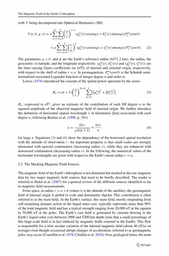
Mathematically, the lithospheric field is the magnetic contribution that remains after sub-traction of the core plus the external fields or sometimes simply a regional trend. The re-maining magnetic signal may be positive in places where it reinforces the ambient field butnegative when it opposes it. From this viewpoint, the magnetism of rocks is carefully definedas an anomaly with respect to the dominant internal and external magnetic fields. This def-inition stresses how difficult it is to ascertain the geophysical origin of the anomalies sincethe accuracy with which the data are corrected for external and core fields has a profoundeffect on them. This lack of clarity can be illustrated in the spectral domain with the Earth’smagnetic field power spectrum ((3) and Fig. 1). The analysis of satellite data shows a breakin slope of the power spectrum (3) between SH degrees 13 and 16 (Langel and Estes 1982).Long-term dynamo processes (the core field and its secular variation) dominate the fieldbetween 40,000-km (SH degree 1) and 3100-km or 2460-km wavelengths (considering theupper or lower limit SH degrees 13 or 16 respectively). Prior to epoch 2000.0, InternationalGeomagnetic Reference Fields (IGRF) models were derived to SH degree 10, and 13 there-after (Langel 1987, Sect. 7; Macmillan 2007) but, in these models, the secular variation istracked to SH degree 8. Only during the last decade, with excellent satellite data coverage,has it become possible to derive core field models to higher resolution; i.e., to at least SH de-gree 16 (e.g. Olsen et al. 2000). When processing datasets collected at different epochs, thedisagreements in main field and secular variation models and their different truncation levelslead to different pictures of the anomaly field. To some extent, a similar problem is causedby ionospheric and FAC currents that, according to Fig. 1, overlap with the lithospheric fieldat medium to short wavelengths. A detailed review discussing the challenge of separatinginternal from external field sources may be found in Olsen et al. (2009b).

These ambiguities in defining and quantifying the lithospheric field are due to its com-plex nature, which reflects the heterogeneous distribution of magnetic minerals in the sub-surface. At the Earth’s surface, the power spectrum of the lithospheric field expressed inSH (3) is almost flat, which crudely means that all spatial scales are equally energetic (Jack-son 1990, 1994). Therefore, a large number of observations covering different spatial rangesand altitudes are needed to depict accurately this source, from local small-scale contributionsto the larger scales of tectonic units.

The Magnetic Field of the Earth’s Lithosphere

Fig. 1 Schematic representation of the power spectra of magnetic field sources at 400 km altitude (left) andtheir spatial location with altitude (right, after Hulot et al. 2007)

4 Near-Surface and Satellite Measurements

Different magnetic measurements that cover different ranges of spatial and time scales(Mandea and Purucker 2005) are available from ground to satellite altitudes. They areall useful for lithospheric field modelling but not always optimised for it. In addition, thelithospheric field requires accurate and high-resolution measurements but their quality andsampling rate depend on technical improvements and innovation in building magnetometers(Turner et al. 2007) as well as on the reduction of the magnetic noise during the surveys oron the precise time and location determination.

4.1 Magnetic Observatory Data and Ground Surveys

Continuous records of three orthogonal components of the magnetic field (and, indepen-dently, the intensity) are available on land at magnetic observatories distributed worldwide(Matzka et al. 2010). These measurements have high quality standards with a typical res-olution of 0.01 to 0.1 nT. Observatories release hourly mean values, some even deliveringone-second data. These ground data are seldom used directly for crustal magnetic field in-vestigation because of their poor spatial coverage. They are, however, ubiquitous at eachstage of the preparation, acquisition, and post-processing of crustal magnetic field surveys(Reeves 2005). Magnetic observatories also monitor in real time the activity of the externalfield to distinguish ‘quiet’ from ‘disturbed’ magnetic times. During quiet times, observa-tory data provide a baseline, allowing the meticulous removal of external field variations ofsmall amplitude that may occur during the data acquisition. Measurements of the seculartime changes of the main magnetic field prior to the satellite era were exclusively based onthe network of magnetic observatories and repeat stations, where ground-based vector mea-surements are scheduled every few years. These repeat stations networks are established ona national or regional basis for updating secular variation maps locally to arguably betterspatial resolution than global models. Although rarely used in this context, repeat stationvector data may be useful in principle to investigate if the crustal field is varying with time.

E. Thébault et al.

4.2 Marine Data Measurements

Magnetic field measurements made at sea were among the first direct measurements of themagnetic field (Jackson et al. 2000). Declination and inclination measurement were carriedout at times when mariners still lacked a reliable method to determine the longitude (Jonkers2000). Nowadays, sea surface marine magnetic surveys are routinely undertaken for min-eral and hydrocarbon exploration, and marine research. Marine measurements are generallyscalar and obtained with a sensor towed behind a ship at a distance large enough to avoidmagnetic field perturbation from the engines. Marine data processing is a tedious task. Be-fore the era of Global Positioning System (GPS), a major issue was to determine accuratelythe location of the ship. Other magnetic field sources of geophysical origin such as main fieldand more importantly rapidly varying external fields are also difficult to remove because ofthe usually large distance separating the ship and the nearest land magnetic observatory.The absence of baseline requires having a few repeated measurements in order to performcrossover analyses, which provide a good measure of the survey accuracy. Current practiceis that a marine magnetic survey is carried out with a nearby temporarily installed ground(or sea floor when possible) base station and typical errors in reducing the data are about10–20 nT, to be compared to about 80 nT for earlier epochs (e.g. Quesnel et al. 2009). Thisuncertainty illustrates the difficulty of extracting the anomaly magnetic field from the rawmeasurements acquired at sea level (e.g. Tivey 2007). After correction for all other magneticfield contributions, marine magnetic anomalies have typical amplitudes ranging between 1and 1000 nT, depending on the depth of the ocean floor, and the maximum resolved spatialwavelength of marine surveys is of the order of 100–200 km.

4.3 Aeromagnetic Data

The magnetic field of the crust has been measured systematically since the 1940s by air-borne surveys supporting mineral and petroleum exploration (Nabighian et al. 2005; Pilk-ington 2007). Most surveys are flown to aid in surface geologic mapping, where the mag-netic effects of geologic bodies and structures can be detected even in areas where rockoutcrop is scarce or absent, and where bedrock is covered by glacial overburden, bodies ofwater, sand, or vegetation. Aeromagnetic surveys are usually flown in a regular pattern ofequally spaced parallel lines (flightlines) perpendicular to the geological strike direction,with some perpendicular and more widely spaced ‘tie lines’. Rapid external field variationsare determined at a base station set up for the survey or at a nearby observatory. For recon-naissance mapping of large regions (e.g. states and countries), where little or no knowledgeof the magnetic field to be mapped is available, typical line spacing is 0.5–1.5 km. Thesurvey altitude is intimately related to flightline spacing with lower altitude being more ap-propriate for closer line spacing. Prior to the availability of GPS navigation, surveys overmountainous regions were flown at a constant altitude. Post-survey processing of the col-lected magnetic field data could then be applied to “drape” artificially the measurementsonto a surface at some specified mean terrain clearance. The final product resulting froman aeromagnetic survey is a set of magnetic field anomaly values interpolated and lev-elled to a common altitude onto a regular grid, and corrected for the main and externalfields. The error arising from a poor estimate of the secular variation becomes visible whenadjacent or overlapping surveys recorded at different epochs are merged. This introducesresidual trends in the data and discontinuities along the survey boundaries. This mergingrequires accurate main field models for all corresponding epochs (e.g., Ravat et al. 2003;Ravat et al. 2009). The typical spatial resolution of aeromagnetic surveys ranges between

The Magnetic Field of the Earth’s Lithosphere

a few hundreds meters to hundreds of kilometres. As is the case for marine measurements,aeromagnetic data are traditionally scalar because the lack of a stable reference frame ren-ders difficult the acquisition of vector measurements.

4.4 Satellite Data

The magnetic signature of large geologic structures with dimensions of a few hundred kilo-metres cannot always be inferred from near-surface measurements because of the smallsurvey dimensions. Large wavelengths could be in principle registered by stratospheric bal-loon at 20 km to 30 km altitude but controlling the airship route is rather challenging andvery few surveys have been carried out in the past using this platform (Cohen et al. 1986). Incontrast, Low Earth Orbiting (LEO) satellites offer superior spatial coverage over near sur-face data and provide the homogeneous datasets necessary to detect and map the large-scalelithospheric magnetic field features (and to represent all other sources, in particular the mainfield and its secular variation that were not monitored in the oceans before the satellite era).Unfortunately, by virtue of (3), the amplitude of small-scale components decreases rapidlyas the altitude of observation increases. At 400 km altitude the lithospheric field is one ofthe weakest detectable sources, where it typically represents less than 0.1% of the full signalwhich raises some difficulties (e.g. Maus et al. 2008).

The first global scale measurements of the magnetic field from satellite (600–1500 kmaltitude) were collected by the POGO satellites between 1967 and 1971 (Regan et al. 1975;Cain 2007). The accuracy of the scalar magnetometer made possible maps of the lithosphericmagnetic field to SH degree 30; i.e. to about 1300 km wavelength but the availability ofscalar measurements only gave rise to an ambiguity defined as the Backus effect (Backus1970). MAGSAT (Langel et al. 1980a; Purucker 2007) was the first satellite measuring themagnetic field with a vector magnetometer in a low orbit (300–550 km). The MAGSATsatellite orbited for seven months. Lithospheric field maps were computed up to SH degree63 (Cain et al. 1989) and established the location of large individual anomalies but theamplitudes of the features varied significantly from map to map. The development of bettercalibration techniques in the following 20 years, and models describing both internal andexternal fields, allowed for the recognition of the first order difference between the strengthof the magnetic field from continental and oceanic crust (Langel and Hinze 1998). Thelaunch of Ørsted (Neubert et al. 2001; Olsen 2007) in 1999 signalled the beginning of the2nd age of magnetic exploration of the Earth’s lithosphere from satellite. In combinationwith the CHAMP satellite (Reigber et al. 2002; Maus 2007) launched the following year,models of the lithospheric field are now available to SH degree 120 from data collectedcontinuously over a decade (Maus et al. 2008). LEO satellites thus currently provide a viewof the Earth’s lithospheric field between 350-km and 3000-km wavelengths. (Note that weare unable to assert that all wavelengths are presently robustly determined.)

A major source of satellite data error is related to the difficulty of calibrating the instru-ments. The absence of baseline control, the misalignment of magnetometers, and attitudeerrors of the spacecraft lead to some inconsistencies between close satellite encounters (e.g.Olsen et al. 2006). With the upcoming launch of the Swarm constellation of three satellites(Friis-Christensen et al. 2006), it is expected that the remaining gaps and mismatch betweenairborne and satellite surveys will be minimized. The simultaneous availability of identicalsatellites flying along different chosen orbits will allow better corrections for external mag-netic field signals and for the East-West horizontal gradient of the Earth’s magnetic field tobe measured.

E. Thébault et al.

5 Mapping the Earth’s Lithospheric Field

The ability of aeromagnetic and marine magnetic surveys to highlight locally and region-ally the geologic entities showing a magnetic contrast with their surroundings has been longexploited. For scientific purposes, it is also important to acquire consistent data over longdistances, in order to evaluate the crustal structures, to understand the geological processesin conjunction with other geophysical information, to establish tectonic models of conti-nental and oceanic crust, to enable palaeo-reconstructions, and to contribute to geodynamicmodels (e.g., Reeves and De Wit 2000). Ideally, such a multi-scale view could be obtainedby compiling together ground, aeromagnetic and marine regional surveys in order to restorethe continental-scale magnetic trends otherwise not visible in individual datasets. We knowthat this is not achievable for the reasons discussed below and that information on part ofthe missing wavelengths, the largest ones, needs to come from satellite data.

5.1 Satellite-Based Lithospheric Field Models

Direct mapping of the lithospheric field by binning satellite data corrected for all otherknown magnetic field sources has been widely used in the past processing of POGO andMagsat data (see Langel and Hinze 1998 for a review) on Earth and more recently with theprocessing of Mars Global Surveyor (MGS) data (Connerney et al. 2005). With the longrunning Ørsted and CHAMP datasets, the simplistic data binning is no longer acceptablebecause of increasing data quality and better understanding of the interaction between thevarious magnetic field sources. Modelling the data is of great importance to separate themagnetic field sources and to challenge our understanding of the Earth’s magnetic field(Hulot et al. 2007). Representing the magnetic vector data with SH (2) facilitates separatingthe internal and external sources, computing the magnetic field vector outside the dominionof the data, accounting for the spatial and time distribution, and performing spectral analysesas well as statistical comparisons between models. All these possibilities provide ultimatelybetter quality control on the models. Two complementary philosophies based upon SH rep-resentation are widely used for representing mathematically the magnetic field of the Earth’slithosphere.

5.1.1 Serial Approach

Since the lithospheric field at satellite altitudes is often regarded as an anomaly field, themost natural approach is to remove sequentially all other known magnetic field contribu-tions. This approach requires data selection and empirical corrections. The first step of theserial approach is to select data that are the least contaminated by external field contribu-tions. Traditionally, external field activity is characterized by magnetic indices derived fromEarth’s magnetic observatories (Mayaud 1980; Siebert and Meyer 1996). Two planetary in-dices, Kp and Dst, measuring the external field activity, are used to select the ‘quietest’data. In addition, the selection of night side data mitigates most of the effects due to diurnalionospheric fields. The division of scalar and vector data into polar and non-polar regions,with vector data for the polar regions excluded, also helps to minimize the error due to polarelectrojets and FAC.

The second step consists of correcting the selected data for the main field and its secularvariation. Over the last decade, the combined analysis of CHAMP and Ørsted satellite dataled to major improvements in models of the Earth’s magnetic field. It has been possible toderive models for the main field and its secular variation to unprecedented accuracy and

The Magnetic Field of the Earth’s Lithosphere

resolution (e.g., Holme et al. 2002; Langlais et al. 2003; Sabaka et al. 2002, 2004). Suchimprovements benefit a wide community of users through the IGRF models regularly pub-lished by IAGA (e.g., MacMillan et al. 2005; Finlay et al. 2010). This, in turn, allows betterreduction of near-surface measurements and improves their consistency.

The relevance of external contributions to internal field modelling was long ago outlinedby Langel et al. (1996) but recent satellite investigations led to a better identification of re-gions where, and local times at which, ionospheric and magnetospheric fields are prominent.Stolle et al. (2006) proposed an automatic procedure to identify the magnetic field contri-bution generated by post-sunset low-latitude ionospheric plasma instabilities. Lühr et al.(2003) established a model for correcting for the diamagnetic effect that occurs around thedip magnetic equator during the hours following sunset at the altitude of the CHAMP satel-lite. Moreover, toroidal currents flow in the F-region of the ionosphere crossing the satelliteorbit (see Heelis 2004); Maus and Lühr (2006) proposed a method for correcting CHAMPsatellite data for them. It is also possible to predict and correct for secondary magnetic fieldssuch as those caused by major oceanic tides (Tyler et al. 2003; Kuvshinov and Olsen 2006).Most of the above-mentioned signals have spatial scales and strength falling in the rangeof lithospheric anomalies. These corrections were not available at the epochs of POGOand Magsat. It is remarkable that this succession of selection and corrections together withthe improvements in satellite magnetometers allowed enhanced lithospheric field resolutionfrom about 650 km (SH degree 63) at the time of Magsat (Cain et al. 1989) to 500 km (SHdegree 80) for the first CHAMP scalar model (Maus et al. 2002). Note that the resolution(the maximum degree of the SH expansion) and the robustness (the maximum SH degreeresolved by the data) of a model should not be confused. As shall be seen in Sect. 5.1.3, themodel of Cain is robustly determined only to up degree, say, 40 so that the improvement inrobustness from Magsat to CHAMP is actually larger than the improvement in resolution.

The most recent model (Fig. 2) further includes along-track corrections, line levellingbetween adjacent satellite tracks (which minimizes the variance between close encounters),and some subtle regularization of the inverse problem. It now extends down to 330 kmwavelength (SH degree 120; Maus et al. 2008) and is claimed to resolve major oceanicmagnetic lineation. However, one should keep in mind that this latter model is regularizedfrom SH degree 80, which means that coefficients for higher degrees are not necessarilywell resolved.

5.1.2 Comprehensive Approach

An alternative approach to serial geomagnetic field modelling has been developed over thepast two decades in order to address the problem of magnetic field sources separation andspectral overlap (Fig. 1). This approach aims at inverting simultaneously various datasetsfor all mathematically described internal and external fields varying in space and time in acomprehensive way. Early attempts to derive comprehensive models (Sabaka and Baldwin1993; Langel et al. 1996) did not describe the lithospheric field sources and represented theexternal fields in a simple way. However, they demonstrated the feasibility of this approachand offered the groundwork for building models that are now more elaborate. CM3 (Sabakaet al. 2002) is built upon a rich dataset including POGO and Magsat satellites as well asground observatory data covering epochs between 1960 and 1985. The lithospheric mag-netic field is described by SH degrees 16 to 65 (down to 615 km wavelength). The mostrecent comprehensive model (CM4; Sabaka et al. 2004) spans the years 1960–2002. Inter-estingly, in spite of the inclusion of more recent CHAMP and Ørsted data, the description ofthe lithospheric field is not considerably improved as it extends to SH degree 65 with prob-ably too much energy in SH degrees 45–65 (Fig. 4). This maximum resolution is less than

E. Thébault et al.

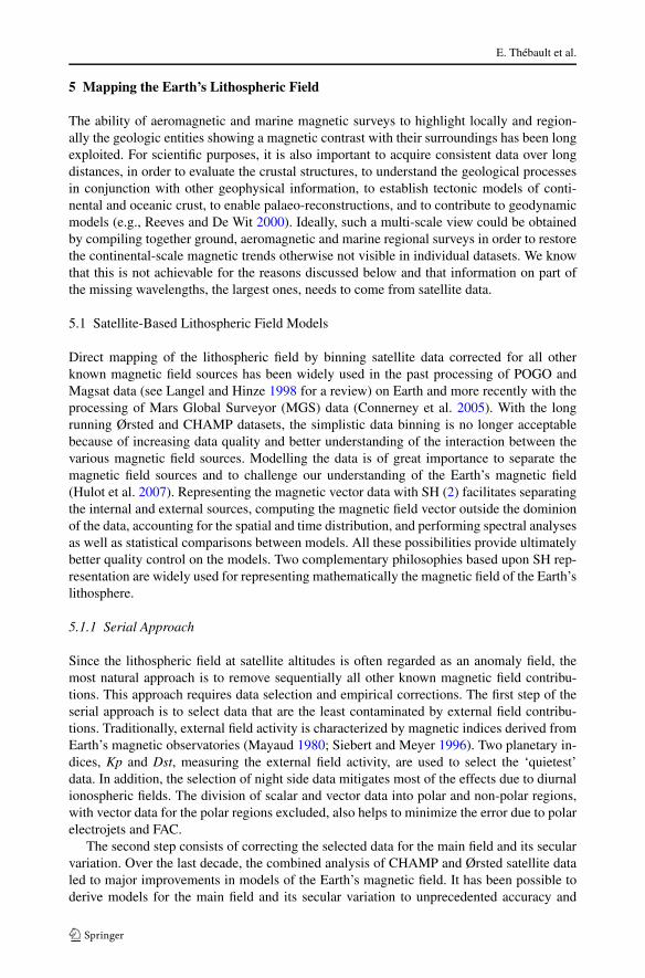
Fig. 2 Vertical component of the MF6 lithospheric field model for SH degrees 16–120 at the Earth’s refer-ence radius (after Maus et al. 2008)

that provided by serial models. In fact, for improved description of external magnetic fieldsources (and their induced counterparts), dayside data must be considered in the compre-hensive scheme. This is a major limiting factor for lithospheric field modelling as daysideexternal fields overlap with the lithospheric field in the spatial spectral domain (Fig. 1). Thissituation illustrates the problem, and the importance, of data selection. Of course, one shouldalso keep in mind that the CM4 model was not derived with the most recent and lowest al-titude CHAMP satellite data. In 2000 the mean altitude of CHAMP was about 460 km andit decreased to 280 km in May 2010 (the mission should be ending at the end of 2010).A noteworthy application of CM4 was to help planning the forthcoming European Swarmsatellite mission (Friis-Christensen et al. 2006) and to optimize the satellites numbers andorbits for exploring the Earth’s magnetic field (Sabaka and Olsen 2006). The simulationsshowed how the three satellites flying in different orbits would provide the desynchronizeddata in space and time (and their gradients) that are necessary to disentangle internal fromexternal field sources in a comprehensive way, with a limited recourse to data selection andcorrection.

Other models include several magnetic field sources but focus more on the main field.The CHAOS (Olsen et al. 2006) and CHAOS-2 (Olsen et al. 2009a) models, and GRIMM(Lesur et al. 2008), for instance, propose different ways of modelling the main field, itssecular variation and acceleration for the past 10 years (2000–2010) but do not resolvethe lithospheric field better than SH degree 40 for CHAOS and degree 60 for GRIMMand CHAOS-2. Other models are hybrid. POMME-3 (Maus et al. 2005), for instance, co-estimates the main field, secular variations and some parameterized external fields with the

The Magnetic Field of the Earth’s Lithosphere

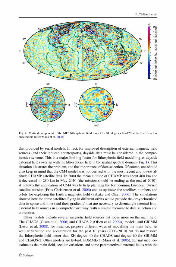
Fig. 3 Vertical component of the CM4 lithopsheric field model for SH degrees 15–45 at the Earth’s referenceradius (after Sabaka et al. 2004)

Fig. 4 Power spectra of differentlithospheric field models usingthe sequential or thecomprehensive approachcalculated at 400 km altitudeabove Earth’s mean radius (afterCA90: Cohen and Achache 1990;CAIN 1989: Cain et al. 1989;CM4: Sabaka et al. 2004;CHAOS-2: Olsen et al. 2009a;MF2: Maus et al. 2002; MF6:Maus et al. 2008)

Dst index split into external and transient internal contributions (Maus and Weidelt 2004) torepresent as accurately as possible the dominant internal and external field sources. Then,serial filtering is performed to extract what is assumed to be the signature of high SH degreelithospheric fields.

E. Thébault et al.

5.1.3 Comparing Comprehensive and Serial Lithospheric Field Models

The comprehensive and the serial approaches do not lead to models of equivalent res-olution or robustness in the waveband between SH degrees 15 and 45 (900–2900 kmwavelength) while all comprehensive approaches give essentially the same picture ofthe lithospheric field. In that respect, comprehensive approaches provide robust but low-resolution lithospheric field models whereas sequential models, while less robust, havehigher resolution. One difficulty is common to all models because the satellite polar gapsleads to inevitable discrepancies (mainly for orders m = 0, see Olsen et al. 2004). Apart fromthis, specific problems are identified when comparing the results of the two approaches.Working with a variety of models, Hemant and Maus (2003) observed systematic loss ofpower for the lithospheric field estimated by serial analysis (see Fig. 4). This observationwas later formally explained by Sabaka and Olsen (2006) to justify the comprehensive ap-proach. Since core and lithospheric fields have a disputed territory in the spectral domain(between SH degrees 13 and 16) within which we cannot discriminate between the twooverlapping sources, removing a main field first will remove power actually belonging tothe lithospheric field. This creates the observed lack of power in sequential types of modelscompared to comprehensive ones (Fig. 4). In a sense, they demonstrate that the lithosphericfield is more than an anomaly field with respect to other contributions.

Another difference appears as North-South features in the residual maps between thevertical components computed with both types of models (Fig. 5). In order to derive alithospheric field with the serial approach, a questionable but necessary step consists offiltering the magnetic measurements along the satellite tracks to eliminate external fields(Maus et al. 2008). This along-track filtering may introduce some artefacts. Cohen andAchache (1994) noticed reduced amplitudes in the Magsat satellite orbit direction afteralong-track correction and raised the question of possible anisotropy introduced in themaps. This effect would be particularly prominent at low SH degrees (Ravat et al. 1995;Purucker et al. 1997). Since some remanent oceanic magnetic field anomalies happen to beelongated in the North-South direction (roughly parallel to the direction of a polar orbitingsatellite), this procedure is also likely to create problems when separating induced from re-manent magnetisation of the Earth’s crust (e.g. Purucker and Whaler 2007) by deleting animportant contribution to remanent magnetism. The stripes in Fig. 5 are also visible overcontinents and appear to be satellite footprints. For this reason, Thébault (2007) interpretedthem as artificial features resulting from spectral leakage introduced by the track-by-trackfiltering. These manufactured features could then be falsely interpreted as ocean floor mag-netic anomalies. It is remarkable that performing the along-track correction at the latest stageof the processing (i.e. after all possible corrections are applied) reduced significantly theseartefacts in MF6 (Maus et al. 2008). The subsequent line levelling and regularization wasthen efficient enough to smooth out the remaining East-West oscillations generated by alongtrack filtering (Fig. 5 bottom).

Comprehensive and serial philosophies should not be considered as competing as theydo not pursue the same aim. There are no better words than those of Langel (1993, p. 48) toillustrate this dual approach : “Until the basic morphology and variability of the individualsources are well understood, it most definitely is more transparent and useful to isolate thefield of interest as much as possible and study it separately”. The sequential approach hasthus to be considered as a first iteration towards a more comprehensive understanding andmodelling of the magnetic field. Figure 4 shows that the mismatch between both types ofmodels has been continuously decreasing during the last decade. More specifically, the se-quential approach seems to converge towards the comprehensive one (for SH degree 15–45).

The Magnetic Field of the Earth’s Lithosphere

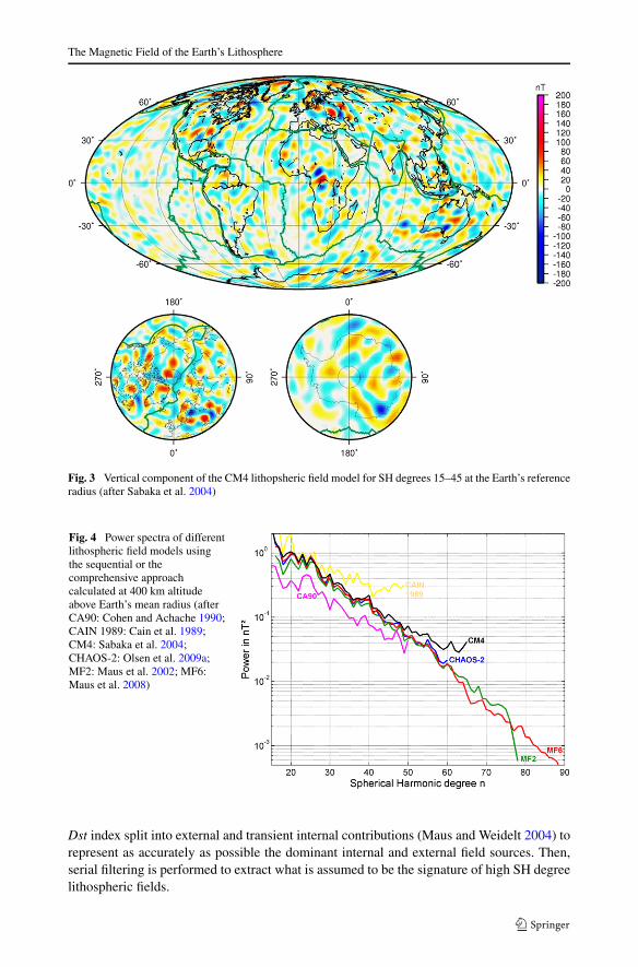
Fig. 5 Vertical component of the difference between MF5 and CM4 (top) and between MF6 and CM4(bottom) for SH degrees 16–45 at Earth’s reference radius

This suggests that if a unique solution to the serial approach existed, it would be equivalentto a comprehensive solution.

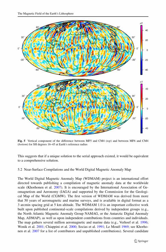
5.2 Near-Surface Compilations and the World Digital Magnetic Anomaly Map

The World Digital Magnetic Anomaly Map (WDMAM) project is an international effortdirected towards publishing a compilation of magnetic anomaly data at the worldwidescale (Khorhonen et al. 2007). It is encouraged by the International Association of Ge-omagnetism and Aeronomy (IAGA) and supported by the Commission for the Geologi-cal Map of the World (CGMW). The first version of WDMAM was derived from morethat 50 years of aeromagnetic and marine surveys, and is available in digital format as a3 arcmin spacing grid at 5 km altitude. The WDMAM 1.0 is an important collective workbuilt upon published continental-scale compilations derived by independent groups (e.g.,the North Atlantic Magnetic Anomaly Group NAMAG, or the Antarctic Digital AnomalyMap, ADMAP), as well as upon independent contributions from countries and individuals.The map gathers several million aeromagnetic and marine data (e.g., Verhoef et al. 1996;Wonik et al. 2001; Chiappini et al. 2000; Socias et al. 1991; Le Mouël 1969; see Khorho-nen et al. 2007 for a list of contributors and unpublished contributions). Several candidate

E. Thébault et al.

grids for the WDMAM were submitted for evaluation and their differences illustrated thedifficulty of merging such a variety of datasets (Hamoudi et al. 2007; Hemant et al. 2007;Maus et al. 2007a).

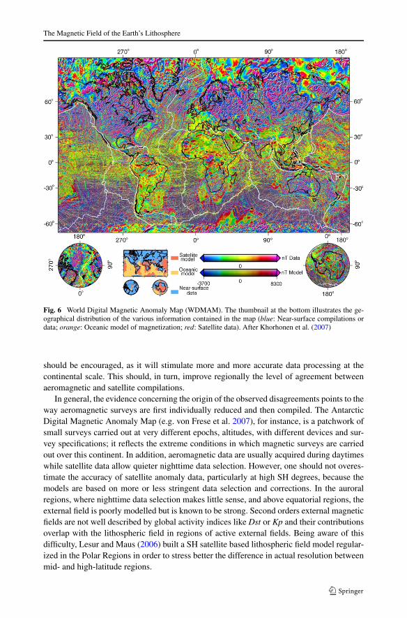
For the purpose of geophysical exploration, the absolute accuracy of measurements is ofrelatively little importance. Only magnetic contrasts matter. Most of the data available forthe WDMAM project were thus provided as anomaly scalar data or grids with their own pro-jection system and reference altitude. Important information related to the quality of eachsurvey and the correction parameters of main and external fields, processing and levellingperformed, were most of the time no longer available. This variety of data reduction andcorrections between survey epochs caused discontinuities between adjacent compilationsand inconsistencies in abutting and overlapping areas. Such disagreements are usually at-tributed to wavelengths down to 400 km, even though smaller scale incompatibilities arealso often present. Fortunately, the longer wavelengths could be filtered out and later re-placed by predictions of a satellite data based global magnetic anomaly field model (Mauset al. 2007b). They could have been replaced with values from a comprehensive model butat the cost of a partial spectral gap between SH degrees 65 and 90. One should thus keep inmind the compromise that was made between resolution and robustness. In particular, thechosen model, MF5 (Maus et al. 2007a), was not completely free of elongated artefacts inthe North-South direction. Empty oceanic areas were further filled in by predictions from alithospheric magnetisation model. The printed WDMAM 1.0 is thus a superposition of dataand models (Fig. 6). In order to improve the compatibility of smaller scale anomalies andtheir identification, continuous efforts are being made to improve the quality and the datacoverage of the WDMAM map (e.g. Gaina et al. 2008; Quesnel et al. 2009). In addition, newdata processing involving prior information based on an oceanic crustal age model (Mülleret al. 2008) has been recently tested and proved to be efficient at interpolating the data be-tween sparse tracklines in the oceans in most parts of the world (Maus et al. 2009) until newmarine data are released or acquired. These new advances will benefit WDMAM 2.0, whichshould be released in 2011.

5.3 Compatibility Between Near-Surface and Satellite Models

The fact that some wavelengths are removed in continental-scale aeromagnetic and marinecompilations requires some more discussion, particularly if a map such as WDMAM is tobe interpreted. Prior to the launch of the Ørsted and CHAMP satellites, and without accu-rate control of the long wavelengths in aeromagnetic surveys (e.g. Tarlowski et al. 1996),there was little overlap between the wavelengths measured by satellite and airborne surveys,or even between the communities involved in their analysis. This problem was thus oftenignored. Yet, Langel et al. (1980b) noticed a lack of compatibility between aeromagneticand satellite data over Canada (that was later confirmed over the same region with moreadvanced processing analysis by Ravat et al. 2002). Schnetzler et al. (1985) faced the sameissue a few years later when comparing a composite magnetic anomaly map and Magsatanomaly data over the contiguous United States. Such investigations were recently revivedwith the release of the WDMAM 1.0. It is now possible to assert that there is indeed a sys-tematic disagreement between near-surface and satellite observations for the power in SHdegrees 15–100. The overall degree of compatibility between near-surface compilations andsatellite models was estimated by Hamoudi et al. (2007) and Maus et al. (2007b, 2009); itrarely exceed 60% on average. In order to investigate the geographical distribution of thecorrelation, new complements of analysis tools have been developed (Maus 2008; Chambo-dut et al. 2008). The systematic analysis of the effective spectral content of each data type

The Magnetic Field of the Earth’s Lithosphere

Fig. 6 World Digital Magnetic Anomaly Map (WDMAM). The thumbnail at the bottom illustrates the ge-ographical distribution of the various information contained in the map (blue: Near-surface compilations ordata; orange: Oceanic model of magnetization; red: Satellite data). After Khorhonen et al. (2007)

should be encouraged, as it will stimulate more and more accurate data processing at thecontinental scale. This should, in turn, improve regionally the level of agreement betweenaeromagnetic and satellite compilations.

In general, the evidence concerning the origin of the observed disagreements points to theway aeromagnetic surveys are first individually reduced and then compiled. The AntarcticDigital Magnetic Anomaly Map (e.g. von Frese et al. 2007), for instance, is a patchwork ofsmall surveys carried out at very different epochs, altitudes, with different devices and sur-vey specifications; it reflects the extreme conditions in which magnetic surveys are carriedout over this continent. In addition, aeromagnetic data are usually acquired during daytimeswhile satellite data allow quieter nighttime data selection. However, one should not overes-timate the accuracy of satellite anomaly data, particularly at high SH degrees, because themodels are based on more or less stringent data selection and corrections. In the auroralregions, where nighttime data selection makes little sense, and above equatorial regions, theexternal field is poorly modelled but is known to be strong. Second orders external magneticfields are not well described by global activity indices like Dst or Kp and their contributionsoverlap with the lithospheric field in regions of active external fields. Being aware of thisdifficulty, Lesur and Maus (2006) built a SH satellite based lithospheric field model regular-ized in the Polar Regions in order to stress better the difference in actual resolution betweenmid- and high-latitude regions.

E. Thébault et al.

5.4 Reconciling Ground and Satellite Data

The WDMAM is a product developed by compiling anomaly intensities seen by satellites,ships and airplanes. A more consistent way of deriving maps or models with the most com-plete magnetic field spectrum could be to merge the complementary information with thecalculation of a model (i.e. to model them jointly). The SH solution of the Laplace equationis not always convenient when the data are not distributed equally at the Earth’s surface orwhen datasets are incompatible globally. Beyond this problem of data distribution, particu-larly troublesome at near-surface altitudes (see legend of Fig. 6), the large number of Gausscoefficients required to represent the field at very short wavelengths is also daunting.

The NGDC720 model (http://www.ngdc.noaa.gov/geomag/EMM/emm.shtml) repre-sents the WDMAM to about 50 km minimum resolution (SH degree 720) and requiresmore than half a million Gauss coefficients. Representing the full WDMAM grid (for spa-tial wavelengths in the range 5 km–3000 km) would require more than 64 million Gausscoefficients (SH degree 8000).

A possible solution to circumvent this issue in regions where ground and satellite dataare reasonably compatible is to favour an approach relying on regional modelling. Severalstrategies based on potential field theory have been, and are still currently being, developed(see Schott and Thébault 2010, for a review). The first series of approaches relies on ba-sis functions with global support, which have their energy optimally concentrated in thespatial and spectral domain corresponding to the region of interest. They may be based onlinear combinations of SH like splines (Shure et al. 1982), band-limited functions (Lesur2006), or Poisson wavelets (Holschneider et al. 2003; Mayer and Maier 2006). Based onthe early work of Constable et al. (1993), Stockman et al. (2009) recently proposed imagingthe Earth’s crustal field measured at satellite altitude with spherical tessellations. Anothermethod using Slepian functions (Simons and Dahlen 2007) is still in its development stagein the framework of geomagnetism (Beggan and Simons 2009).

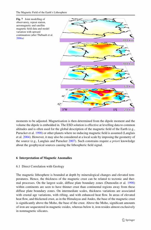
The second type of approach uses basis functions with local support. Common tech-niques, like polynomial modelling in latitude and longitude, rectangular harmonic analysis(Alldredge 1981), or spherical cap harmonics (Haines 1985) often used in the past (Tortaet al. 2006), should not be used when data are available at different altitudes (Mandea andPurucker 2005; Thébault and Gaya-Piqué 2008; Schott and Thébault 2010). The RevisedSpherical Cap Harmonic Analysis, R-SCHA (Thébault et al. 2004, 2006a; Thébault 2008),is a regional method specifically derived for modelling magnetic data collected at variousaltitudes. An example of its application is the merging of vector and scalar repeat station,observatory, aeromagnetic and satellite data for modelling the lithospheric fields of France(Fig. 7) and Germany to 30 km resolution (Thébault et al. 2006b; Korte and Thébault 2007).Even though this is not the primary aim of the technique, a lithospheric field model us-ing CHAMP satellite data was derived by stitching together independent regional models(Thébault 2006). Note that this regional modelling technique does only yield a satisfactorysolution if all datasets are compatible, which is obviously a desired property (Thébault andGaya-Piqué 2008). Since data incompatibility is an issue often encountered when mergingnear-surface and satellite measurements (e.g. Ravat et al. 2002) any regional modeling witha similar property may provide insight into the regional level of compatibility between thesetwo particular data types.

Finally, we classify the equivalent source dipole (ESD) technique, introduced by Mayhew(1979), as a forward modelling method intermediate between global and regional modelling.The ESD method assumes a distribution of dipolar sources within the Earth’s crust. Forpurely induced magnetisation, these dipoles are aligned with the main field leaving only their

The Magnetic Field of the Earth’s Lithosphere

Fig. 7 Joint modelling ofobservatory, repeat station,aeromagnetic and satellitemagnetic field data and modelvariation with upwardcontinuation (after Thébault et al.2006a)

moments to be adjusted. Magnetisation is then determined from the dipole moment and thevolume the dipole is embedded in. The ESD solution is effective at levelling data to commonaltitudes and is often used for the global description of the magnetic field of the Earth (e.g.,Purucker et al. 1998) or other planets where no inducing magnetic field is assumed (Langlaiset al. 2004). However, it may also be considered at a local scale by imposing the geometry ofthe source (e.g., Langlais and Purucker 2007). Such constrains require a priori knowledgeabout the geophysical sources causing the lithospheric field signal.

6 Interpretation of Magnetic Anomalies

6.1 Direct Correlation with Geology

The magnetic lithosphere is bounded at depth by mineralogical changes and elevated tem-peratures. Hence, the thickness of the magnetic crust can be related to tectonic and ther-mal processes. On the largest scale, diffuse plate boundary zones (Dumoulin et al. 1998)within continents are seen to have thinner crust than continental regions away from thesediffuse plate boundary zones. On intermediate scales, thickness variations are associatedwith crustal age variations, with rifting, and with enhanced heat flow. In areas of elevatedheat flow, and thickened crust, as in the Himalayas and Andes, the base of the magnetic crustis significantly above the Moho, the base of the crust. Above the Moho, significant amountsof iron are sequestered in magnetic oxides, whereas below it, iron resides almost exclusivelyin nonmagnetic silicates.

E. Thébault et al.

However, evidence that points to the presence of magnetised material in subduction mar-gins within the upper mantle (Blakely et al. 2005) continues to accumulate. Subductingoceanic slabs release water into overlying continental mantle, thereby transforming peri-dotite into serpentinite. Serpentinite is often highly magnetic because of the formation ofmagnetite during the reaction of peridotite with water, and thermal models suggest that thecold, descending slab cools the mantle to below the Curie temperature of magnetite. Withthe notable exception of the Andes, magnetic and gravity anomalies are common over sub-duction zones (e.g. Purucker and Ishihara 2005). In the Cascadia and Alaskan subductionzones, these long-wavelength anomalies have been shown to have source depths within themantle (Blakely et al. 2005). Because hydrated mantle responds differently to deformationthan un-hydrated mantle, and because water released from the slab promotes brittle fail-ure within the slab, models predict a causal connection between intraslab earthquakes andhydrated forearc mantle. This has important implications for seismic risk assessment.

Tectonic processes are responsible for the creation, destruction, and mobilization of mag-netic materials within the lithosphere of the Earth. In the near surface, volcanism and relatedigneous processes such as dike emplacement, rifting, and faulting act to modify pre-existingmagnetic signatures, thus providing critical details of the processes involved. Maps andmodels derived as described in the previous sections may thus be directly compared to theknown geology although interpretations are non-unique and often oversimplified.

6.2 The Sources of the Lithospheric Field at Satellite Altitudes

Representing magnetic field measurements with potential field methods provides modelsthat are important to ascertain to the authenticity of magnetic field features. Likewise, visualinspections provide qualitative insight into the consistency between magnetic anomalies andthe known geology. However, both approaches say little about the physical parameters of thesources, except maybe in the former case by testing statistical descriptions of the distributionof magnetisation against anomaly power spectra (Jackson 1994; Voorhies et al. 2002).

Quantitative magnetic interpretation involving other geophysical quantities such as ge-ology, gravity, seismicity, heat flow, depth to the Moho etc. can be provided by forwardmodelling methods. Meyer et al. (1983) and Hahn et al. (1984), for instance, compared thelithospheric field predicted by a global equivalent distribution of dipoles with the one mea-sured by the satellite Magsat. They were then able to make spectral comparisons betweenthe measured and the predicted lithospheric field models. In their approach, each node of thegrid represents a dipole directed along the main field with a susceptibility value that dependson the crustal type at the location of the node. The crustal types were directly obtained froma classification based on surface geology and seismic information. Following these earlyworks, Nolte and Siebert (1987) derived analytical formulas to express directly the suscep-tibility k (recall (5)) in spherical harmonics (2) and related this quantity to the dipole partof the main inducing magnetic B also expressed in spherical harmonics. With these formu-lae Counil et al. (1991) computed the magnetic field that would be induced by a thicknesscontrast between continental (∼40 km) and oceanic (∼7 km) crust of uniform suscepti-bility value. From this, they predicted that some of the large anomalies recorded by satel-lites would be at continent-ocean boundaries, and confirmed that magnetic crustal thicknessplays a significant role in the dichotomy between oceanic and continental magnetic signalsobserved at satellite altitudes (see also Arkani-Hamed 1993). Cohen and Achache (1994)refined the analysis and included a model of oceanic bathymetry to predict the magneticanomalies over oceanic plateaus. Remanent magnetism in the oceans was later predictedby Dyment and Arkani-Hamed (1998) using the digital age map of ocean floor (Müller

The Magnetic Field of the Earth’s Lithosphere

et al. 1997) and appeared to correlate well with magnetic anomalies over superchrons in theNorth Atlantic and Indian oceans. Hemant and Maus (2005a) synthesised these studies in aunique equivalent dipole model. They predicted the lithospheric magnetic field anomalies at400 km altitude with the help of a map of vertically integrated susceptibility values (VIS).They concluded that magnetic anomalies at the ocean-continent boundaries as predicted byCounil et al. (1991) are too weak to be measured at satellite altitudes in places where theoceanic crust is flanked by young continental provinces (Phanerozoic in age) because thesusceptibility of the oceanic and continental crust there is comparable (Hemant and Maus2005b).

6.3 A Practical Example of ESD Modelling

A practical example of inversion using the ESD procedure together with recent CHAMPsatellite data is illustrated in Fig. 8. The ESD method directly relates anomaly maps toa discrete magnetisation distribution that may be combined with other geological or geo-physical information in the sub-surface. The ESD is usually applied to a large region (oreven globally). The method requires a starting model to set up a priori the Curie depth,here the global seismic 3SMAC (Nataf and Ricard 1996, supplemented by Chulick andMooney 2002) compositional and thermal model of the crust and mantle. Following Counilet al. (1991), a constant magnetic susceptibility (k = 0.04 in (5)) for both oceans and conti-nents is further assumed. The magnetic crustal thickness and the average susceptibility arethen used to predict the magnetic field at satellite altitude. A unique solution is obtainedby further assuming that induced magnetisations dominate over remanent magnetisations incontinental crust, and that vertical thickness variations dominate over lateral susceptibilityvariations (Purucker et al. 2002; Purucker and Whaler 2007). The a priori model of themagnetic crustal thickness provided by 3SMAC is then modified in an iterative fashion untilthe magnetic field predicted by the model matches the observed magnetic field (chosen tobe the satellite magnetic field map of the lithosphere model MF6 of Maus et al. 2008) towithin some specified error. The solution shown in Fig. 8 fits the MF6 lithospheric magneticfield magnetic model to better than 1 nT. We thus obtain an estimate of the magnetic crustalthickness of the continents.

The utility of such ESD modelling becomes clearer when comparing the final magneticthickness and the basement age maps. The basement age map is based on surface and sub-surface observations extended using seismic data, which cover much of the Earth’s surfacebut with significant gaps (cf. Fig. 11 of Mooney 2007). Seismic data are spatially hetero-geneous and of widely different quality. In contrast, satellite magnetic data are spatiallyhomogeneous away from the high latitude auroral zones. Yet models of both data types havecomparable resolution (333 km wavelength) and so are amenable to direct comparison. Sim-ilarities between them include the marked difference between the Eastern European cratonand the younger Variscan terrain to the west. In general, magnetic crust with thicknessesof 16–27 km is associated with basement ages younger than Paleozoic. Exceptions are notuncommon, and one of the most striking is found in South Africa near the coast. Terrainswith marked thickness contrasts within a short distance, as in the southeast United States,often signal the presence of problems with the starting model. This thickness contrast dra-matically decreases if the starting crustal thickness model has the boundary between thickerolder crust, and younger thinner crust, moved to the Fall Line (Purucker et al. 2002). Themaps differ in their assessment of the size of some of the older continental cores, for examplethe Omolon in eastern Siberia (Fig. 8). The magnetic map suggests a much larger subsurfaceextent for this poorly surveyed province. Small older terrains set within younger ones often

E. Thébault et al.

Fig. 8 Magnetic thickness of continental crust (updated from Purucker et al. 2007) compared to basementage (Mooney 2007). Basement age is determined from surface and subsurface measurements, and extrapo-lated under cover rocks using seismic measurements. Oceanic crust is masked on the magnetic thickness mapbecause magnetisations are dominated there by remanent magnetisations. Also masked are two continentalregions associated with the Bangui (1) and Kursk (2) anomalies, where remanent magnetisations, and/or en-hanced magnetic susceptibilities, are known to dominate the magnetic signal. On the magnetic thickness map,3 locates the Omolon terrain of Siberia

show up clearly, as for example the Colorado Plateau and the Tarim Basin. An alternativeinterpretation of the magnetic field observations would relate them to enhanced magneticsusceptibilities (Hemant and Maus 2005a), which in turn implies compositional differences.In the case of the Colorado Plateau, crustal compositions, as inferred from seismic velocitiesby Parsons et al. (1996), appear to be the same beneath the Colorado Plateau and the Basinand Range Province to the southwest, suggesting that magnetic thickness variations domi-nate over susceptibility variations in this region (Purucker et al. 2007). In other locations,we might expect that susceptibility variations would dominate over magnetic thickness.

From the estimate of the magnetic crustal thickness, it is also possible to go a step furtherand to approximate the average heat flow (Fox Maule et al. 2005). This requires simplify-ing assumptions about the thermal state of the continental crust and another starting model

The Magnetic Field of the Earth’s Lithosphere

to constrain the longest wavelengths of the lithospheric field, in excess of SH degree 15(∼2900 km), which are dominated by core field processes (Purucker and Whaler 2007).

An alternative inverse modelling strategy that has been applied to global magnetisationmodelling finds spatially continuous magnetisation models (Whaler and Purucker 2005) in-stead of a discrete set of magnetisations as provided by ESD. Comparisons between globalmodels produced by the two methods are favourable. However, a disadvantage of the con-tinuous magnetisation approach is that the magnetized layer is assumed to have constantthickness, whereas expected variations in depth to Curie isotherm can be incorporated intothe volumes specified for ESD modelling. In practice, this does not make much differenceat satellite altitudes from which the magnetized crust appears as a thin sheet of integratedmagnetic susceptibility but it may be a limiting factor when processing lower altitude data.

6.4 Inherent Ambiguities

As has been discussed in previous sections, comparisons with geology are subject to inherentambiguities. The first ambiguity comes from the fact that some distributions of magnetisa-tion give rise to magnetic fields vanishing above the surface. Such invisible distributions ofmagnetisation are known as magnetic annihilators. Runcorn (1975), for instance, demon-strated that a spherical shell of constant susceptibility produces no field outside of the shell.This ‘shell’ theorem is slightly modified in the case of the Earth’s ellipticity (Jackson et al.1999; Lesur and Jackson 2000). Maus and Haak (2003) found another class of annihilatorssymmetric along the magnetic equator for an Earth’s dipole-dominated inducing field. Theyshowed that a continental scale constant susceptibility distribution over the South Americanand African continents would produce almost no magnetic anomaly. The magnetic anom-alies, in particular, would be invisible along the magnetic equator. For this reason, geologicalfeatures do not always have their magnetic counterpart.

The second ambiguity results from compromises made to interpret the magnetic anom-alies. The inverse problem for magnetisation has particularly severe non-uniqueness, in thesense that no unique interpretation is possible. For instance, even if magnetisation is re-stricted to be purely induced, an increase in crustal thickness can produce a similar signal toa lateral variation of magnetic susceptibility of rocks. One often has to decide which parame-ter (thickness or lateral susceptibility variation) dominates over the other. Mathematically,unique solutions are obtained by imposing an additional constraint such as finding the modelwith minimum root-mean-square magnetisation amplitude for a given fit to the data, eitherimplicitly (ESD) or explicitly (continuous models) (see Whaler and Langel 1996). Ampli-tudes must reach the ‘Parker bound’ somewhere within the magnetised region (Parker 2003);in practice, models providing a ‘reasonable’ fit to the data seem to satisfy the bound easily,except in few places shown in Fig. 8 by areas with dark colour codes where the hypothesisof induced lithospheric field fails.

Since we measure the magnetic fields resulting from magnetisation rather than magneti-sation itself, it is difficult to resolve the field into its induced and remanent components.Any rock exhibits a portion of magnetisation under the influence of the present geomagneticmain field, the induced one, and some indication of past geomagnetic fields, the remanentpart. Figure 9 shows that, if not constrained to be purely induced, the inverse algorithm al-lows a substantial remanent component (nearly 50%). However, equivalent source dipolemodelling comparisons show that data can be fit almost as well with purely induced mag-netisation (even over the oceans) as is illustrated by the work of Hemant and Maus (2005a);a formal statistical test is complicated by the extra free parameters (dipole directions) neededto describe directions as well as amplitudes.

E. Thébault et al.

Fig. 9 Magnetisation (at 20 kmdepth in an assumed 40 km thickmagnetised layer) in the directionof the main field (top),perpendicular to the main field inthe meridian plane (middle) andperpendicular to the meridianplane (bottom) for a continuouslyvarying magnetisation modelobtained using the method ofWhaler and Purucker (2005)from 3-component anomaly datasynthesised at 300 km altitudefrom the MF6 model of Mauset al. (2008)

In principle, induced and remanent magnetisation can be separated because the magneticfield arising from remanent magnetisation is constant over geological times (ignoring chem-ical alteration, and other processes that modify the remanent component), whereas inducedmagnetisation changes as the inducing main field changes over historical times. However,the induced field in the lithosphere is such a small fraction of the inducing core field (whosevarying contribution of 40 nT/yr, on average, is itself low) that it should take many years fora significant change to occur. Goldstein and Ward (1966) attempted to use micropulsations(naturally occurring external field variations of frequency ∼0.1 Hz) to distinguish locallybetween induced and remanent magnetisation. More recently, Clark et al. (1998) extendedthe method to work on differential vector magnetometer data. A different approach was em-ployed by Lesur and Gubbins (2000) who modelled long-running geomagnetic observatoryrecords. Whilst they were unable to resolve unambiguously the induced and remanent com-ponents, they did find a statistically significantly improved fit when a time-varying induced

The Magnetic Field of the Earth’s Lithosphere

component was included. Demetrescu and Dobrica (2005) claimed to have identified thetime-varying induced crustal field at 8 observatories worldwide from an 100–150 years timeseries of annual means. Finally, computing the difference between models based on Magsat(Maus 2007) and Ørsted (Olsen 2007) satellite measurements, Mandea and Langlais (2002)observed unexplained variations of magnetic observatory crustal biases. From the suscep-tibility distribution derived by Hemant and Maus (2005a), Thébault et al. (2009) predictedthat the time-varying induced field should have strength in the range 0.06 and 0.12 nT yr−1

at the Earth’s surface for spatial wavelengths between 440 km and 2700 km. The absolutemaximum of 1.3 nT yr−1 in South America and the relative high of 0.6 nT yr−1 in North-ern Europe are one order of magnitude lower than quantities reported by Demetrescu andDobrica (2005). However, these studies do not investigate the same spatial scales. Hulotet al. (2009) noted that the spectrum of time-varying induced field has the same shape asthe lithospheric field itself with some proportionality factor of (1000 yr)2. This correspondsto a root-mean-square secular variation of the crustal field of about 0.1% per year as waspreviously inferred by McLeod (1996). According to Fig. 6, it may be envisaged that such asmall fraction could nevertheless be large enough to be detected after several years in placesof locally strong magnetic anomalies, provided they are induced. Continuous measurementsnear, or over, identified geological bodies bearing large lateral magnetic susceptibility vari-ations are needed to detect the time variation of the lithospheric field (e.g. Jackson 2007).This requirement is usually not met because magnetic observatories are generally installedin magnetically quiet areas. In addition, dense continuous surface repeat surveys are rareand their accuracy is not sufficient.

A last problem, when interpreting magnetic anomaly maps, occurs because of the mask-ing of the lithospheric contributions by the Earth’s main field (for SH degrees 1 to 13–16).This means that the lithospheric field length scales larger than 2500 km remain unknown;even though forward problems (Cohen 1989), inverse problems (Purucker et al. 1998; He-mant and Maus 2005a, 2005b), and statistical analyses (Jackson 1994) have been undertakenin an attempt to quantify them. These missing continental-scale dimensions manifest them-selves as edge effects along the ocean-continent boundaries and spread over long distances.They may easily be misinterpreted as an effect of local sources when deriving magnetisationand magnetic crustal thickness maps.

7 Conclusions and Outlooks

The magnetic field of the Earth’s lithosphere is a measured quantity from ground, airplanes,ships and space. It is related to various geophysical processes, making these kinds of surveyof great use in research and resource exploration. However, this field is difficult to deduceaccurately and integrally from the available measurements. Aeromagnetic and satellite dataprovide a complementary but incomplete view of the lithospheric field. On the one hand,ground and near-surface measurements have high spatial resolutions but are too close to thesources to provide an extensive lateral view of the magnetic field. On the other-hand, far-fieldmeasurements from space miss the small-scale details and display a comparatively weak andlarger-scale lithospheric field sometimes overwhelmed by closer ionospheric sources. Wethus remain partly blind for the intermediate wavelengths, say between 200 km and 400 km,and the missing dimensions prevent us from probing the entire thickness of the magneticlithosphere. One purpose of the Swarm satellite mission is to partially bridge this gap (Friis-Christensen et al. 2006). In the meantime, significant efforts are still being made to improveour models with satellite data on the one hand, and near-surface data on the other hand; i.e.at both ends of the lithospheric field spectrum.

E. Thébault et al.

The interpretation of this magnetic field is also challenging, both because the magneticfield is subject to inherent theoretical ambiguities, and because there is no general physi-cal description of the Earth’s magnetic crust. Investigations of the Earth’s crust have longshowed that it is a heterogeneous medium. This characteristic is reflected in the fact thatit is not possible to foresee, even crudely, the local or regional magnetic field structuresof the crust. A possible way to predict this field is to consider the Earth’s lithosphere asendowed with average physical properties. This requires studies to be made at satellite al-titude, which as one can realize by comparing Figs. 2 and 6 is incomplete and the resultsare strongly dependent on hypotheses made. For this reason, scientists are also developingnew strategies based on regional modelling approaches and spectral tools to compensate forglobal assumptions. However, these local analyses will always systematically require othergeophysical information to levy ambiguities.

Although the Earth is not the only planet of the solar system with a magnetisedlithosphere (Langlais et al. 2009), the complexity of its magnetic sources and interactions,and the variety of measurements, makes it unique for developing models and understandingthe extent to which the lithospheric field may be interpreted. However, the experience gainedfrom geo- and planetary magnetism is reciprocal as studies of planetary magnetic fields maysupply important information regarding Earth history, which has been irretrievably lost byplate tectonics.

The magnetic field of Mars, for instance, was first recorded by a fly-by in 1965 (Smithet al. 1965), but its lithospheric origin was confirmed much later, in 1997 thanks to themeasurements made on board the orbiting MGS satellite (Acuña et al. 1999). They re-vealed a lithospheric magnetic field of remanent origin, one to two orders of magnitudelarger than the terrestrial one at spacecraft altitude, and whose origin is still highly de-bated. In addition, they gave a picture of SH degrees 1 to 15 for the first time as Marsis devoid of core magnetic field. The Moon too possesses a magnetic field of lithosphericorigin, as was revealed during the initial US-Soviet lunar exploration, but it has two tothree orders of magnitude less power than the terrestrial one. As for Mars, global mea-surements came only recently, during the Lunar Prospector mission (Binder 1998). Venusdoes not seem to posses any internal magnetic field, and no magnetic field associatedwith lithospheric wavelengths has been detected around Mercury so far (Purucker et al.2009) although this can not be formally excluded (Aharonson et al. 2004). Smaller ob-jects have also been studied, such as Braille, a km-scale asteroid. Deep Space 1 flew asclose as 28 km to it and measured a very weak magnetic field, giving a maximum limitof 0.028 A m2 kg−1 for the magnetisation (Richter et al. 2001). Similarly, the NEAR mis-sion flew around 433 EROS, a 10-km dimension body. The very weak magnetic field itrecorded gave a very low limit for Eros’ magnetisation, of the order of 10−6 A m2/kg(Acuña et al. 2002). Satellites of the Jovian system also possess an intrinsic magnetic field.Among others, Ganymede’s magnetic field is presumably associated with an internal dy-namo but influenced by Jupiter’s strong field pervading it. A superposing lithospheric sig-nature is not impossible (Crary and Bagenal 1998). To first order, the lithospheric mag-netic field strength depends on the amount of magnetic material (Langlais et al. 2009;Purucker et al. 2009).

These observations emphasize one important challenge when dealing with planetarymagnetic fields. In contrast to the Earth, one must rely solely on remote measurements madeon board fly-bys or orbiting spacecrafts. This makes the separation of the various magneticfield sources more difficult. Along-track filtering, or SH modelling along a single track ora few flybys, is a procedure widely applied in planetary magnetism (e.g. Purucker 2008)due to the scarcity of available data. In the case of various magnetic field source contribu-tions, their separation is therefore difficult (see Ness 2009). On Mars, for instance, MGS

The Magnetic Field of the Earth’s Lithosphere

provided complete and repeated coverage of the surface at an altitude of about 400 km,at 2:00 am and 2:00 pm local time. These measurements were thus synchronized with lo-cal times and acquired above the Martian atmosphere, where local electric currents createsecondary magnetic fields. The large lithospheric fields on Mars create in turn so-calledmini magnetospheres. Magnetic measurements have therefore to be carefully processed andscreened if one wants to better characterize the magnetic field of lithospheric origin. Ad-ditional measurements are required to quantify the temporal variation of the field. Progresswill be possible using very low altitude (Leblanc et al. 2009) or even surface measurements,such as those provided by aeromagnetic surveys or deployment of a surface geophysical net-work (Lognonné et al. 2000). As is the case for the Earth, this combination of ground andsatellite data would help better discriminating between static and dynamic magnetic fieldsand certainly offer completely different pictures of the lithospheric field.

Acknowledgements We would like to acknowledge R. Balogh and the staff at ISSI, Bern, for organizing asuccessful workshop on terrestrial magnetism as well as Nils Olsen who made a thorough review of this man-uscript. K. Whaler was partly supported by NERC grant NER/O/S/2003/00674. For IPGP, this is contributionnumber 2649.

References

M.H. Acuña, J.E.P. Connerney, N.F. Ness, R.P. Lin, D. Mitchell, C.W. Carlson, J. McFadden, K.A. Anderson,H. Rème, C. Mazelle, D. Vignes, P. Wasilewski, P. Cloutier, Global distribution of crustal magnetisa-tion discovered by the Mars global surveyor MAG/ER experiment. Science 284 (1999). doi:10.1126/science.284.5415.790

M.H. Acuña, B.J. Anderson, C.T. Russell, P. Wasilewski, G. Kletetshka, L. Zanetti, N. Omidi, NEAR Mag-netic field observations at 433 Eros: first measurements from the surface of an asteroid. Icarus 155(2002). doi:10.1006/icar.2001.6772

O. Aharonson, M.T. Zuber, S.C. Solomon, Crustal remanence in an internally magnetized non-uniform shell:a possible source for Mercury’s magnetic field? Earth Planet. Sci. Lett. 218, 261–268 (2004)

L.R. Alldredge, Rectangular harmonic analysis applied to the geomagnetic field. J. Geophys. Res. 86(B4),3021–3026 (1981)

J. Arkani-Hamed, The bulk magnetization contrast across the ocean-continent boundary in the east coast ofNorth America. Geophys. J. Int. 115, 152–158 (1993)

G. Backus, Non-uniqueness of the external geomagnetic field determined by surface intensity measurements.J. Geophys. Res. 75, 6337–6341 (1970)

G. Backus, R. Parker, C. Constable, Foundations of Geomagnetism (Cambridge University Press, Cambridge,1996)

W. Baumjohann, R. Nakamura, Magnetospheric contributions to the terrestrial magnetic field, in Treatise onGeophysics, ed. by M. Kono, vol. 5 (Elsevier, Amsterdam, 2007), pp. 77–91. Chap. 3

C. Beggan, F. Simons, Reconstruction of bandwidth-limited data on a sphere using Slepian functions: ap-plications to crustal modelling. International Association of Geomagnetism and Aeronomy. Abstract#0728, 2009

A.B. Binder, Lunar prospector: overview. Science 281, 1475–1476 (1998)R.J. Blakely, T.M. Brocher, R.E. Wells, Subduction-zone magnetic anomalies and implications for hydrated

forearc mantle. Geology 33, 445–448 (2005)J.C. Cain, Pogo (OGO-2, -4 and -6 spacecraft), in Encyclopedia of Geomagnetism and Paleomagnetism, ed.

by D. Gubbins, E. Herrero-Bervera (Springer, Dordrecht, 2007), pp. 828–829J.C. Cain, Z. Wang, C. Kluth, D.R. Schmitz, Derivation of a geomagnetic model to n = 63. Geophys. J. 97,

431–441 (1989)A. Chambodut, M. Hamoudi, E. Thébault, V. Lesur, Spectral analysis of the world digital magnetic anomaly

map. Abstract#EGU2008-A-09882, EGU, Vienne, 2008M. Chiappini, A. Meloni, E. Boschi, O. Faggioni, N. Beverini, C. Carmisciano, I. Marson, On shore–off shore

integrated shaded relief magnetic anomaly map at sea level of Italy and surrounding areas. Ann. Geofis.43, 983–989 (2000)

G.S. Chulick, W.D. Mooney, Seismic structure of the crust and upper most mantle of North American andadjacent oceanic basins: a synthesis. Bull. Seismol. Soc. Am. 92, 2478–2492 (2002)

E. Thébault et al.

A. Chulliat, E. Thébault, G. Hulot, Core field acceleration pulse as a common cause of the 2003 and 2007geomagnetic jerks. Geophys. Res. Lett. 37, L07301 (2010). doi:10.1029/2009GL042019

D.A. Clark, P.W. Schmidt, D.A. Coward, M.P. Huddleston, Remote determination of magnetic propertiesand improved drill targeting of magnetic anomaly sources by differential vector magnetometry. Explor.Geophys. 29, 312–312 (1998)

Y. Cohen, Traitements et interprétations de données spatiales en géomagnétisme: étude des variations latéralesd’aimantation de la lithosphère terrestre. Thèse de l’Université de Paris, 1989, 95 pp.

Y. Cohen, J. Achache, New global vector magnetic anomaly maps derived from Magsat data. J. Geophys.Res. 95(B7), 10783–10800 (1990)

Y. Cohen, J. Achache, Contribution of induced and remanent magnetisation to long-wavelength oceanic mag-netic anomalies. J. Geophys. Res. 99, 2943–2954 (1994)

Y. Cohen, M. Menvielle, J.L. Le Mouël, Magnetic measurements aboard a stratospheric balloon. Phys. EarthPlanet. Inter. 44, 348–367 (1986)

J.E.P. Connerney, M.H. Acuña, N.F. Ness, G. Kletetschka, D.L. Mitchell, R.P. Lin, H. Rème, Tectonic impli-cations of Mars crustal magnetism. Proc. Natl. Acad. Sci. 102 (2005). doi:10.1073/pnas.0507469102

C. Constable, R. Parker, P. Stark, Geomagnetic field models incorporating frozen-flux constraints. Geophys.J. Int. 113, 419–433 (1993)

J. Counil, Y. Cohen, J. Achache, The global continent–ocean magnetisation contrast: spherical harmonicanalysis. Earth Planet. Sci. Lett. 103, 354–364 (1991)

V. Courtillot, J. Ducruix, J.L. Le Mouël, Sur une accélération récente de la variation séculaire du champmagnétique terrestre. C.R. Acad. Sci. Paris (D) 287, 1095–1098 (1978)

F.J. Crary, F. Bagenal, Remanent ferromagnetism and the interior structure of Ganymede. J. Geophys. Res.103, 25757–25774 (1998)

C. Demetrescu, V. Dobrica, Recent secular variation of the geomagnetic field. New insights from long seriesof observatory data. Rev. Roum. Géophys. 49, 63–72 (2005)

C. Dumoulin, D. Bercovici, P. Wessel, A continuous plate-tectonic model using geophysical data to estimateplate-margin widths, with a seismicity-based example. Geophys. J. Int. 133, 379–389 (1998)

D.J. Dunlop, O. Özdemir, Magnetisations in rocks and minerals, in Treatise on Geophysics, ed. by M. Kono,vol. 5 (Elsevier, Amsterdam, 2007), pp. 278–331. Chap. 8

J. Dyment, J. Arkani-Hamed, Contribution of lithospheric remanent magnetisation to satellite magnetic anom-alies over the world’s oceans. J. Geophys. Res. 103, 15423–15441 (1998)

C.C. Finlay, S. Maus, C.D. Beggan, T.N. Bondar, A. Chambodut, T.A. Chernova, A. Chulliat, V.P. Golovkov,B. Hamilton, M. Hamoudi, R. Holme, G. Hulot, W. Kuang, B. Langlais, V. Lesur, F.J. Lowes, H. Luhr,S. Macmillan, M. Mandea, S. McLean, C. Manoj, M. Menvielle, I. Michaelis, N. Olsen, J. Rauberg,M. Rother, T.J. Sabaka, A. Tangborn, L. Tøffner-Clausen, E. Thébault, A.W.T. Thomson, I. Wardinski,Z. Wei, T.I. Zvereva, International geomagnetic reference field: the eleventh generation. Geophys. J. Int.(2010, submitted)

C. Fox Maule, M. Purucker, N. Olsen, K. Mosegaard, Heat flux anomalies in Antarctica revealed by satellitemagnetic data. Science 309, 464–467 (2005)

E. Friis-Christensen, H. Lühr, G. Hulot, Swarm: A constellation to study the Earth’s magnetic field. EarthPlanets Space 58(4), 351–358 (2006)

C. Gaina, S. Werner (CAMP-GM group), Circum-arctic mapping project: new magnetic and gravity anomalymaps of the Arctic, in 33rd IGC, Oslo, Norway, 2008

C.F. Gauss, Allgemeine Theorie des Erdmagnetismus, in Resultate aus den Beobachtungen des magnetischenVereins im Jahre 1838, ed. by C.F. Gauss, W. Weber (Leipzig, 1839), pp. 1–57

N.E. Goldstein, S.H. Ward, The separation of remanent from induced magnetism in situ. Geophysics 31,779–796 (1966)

A. Hahn, H. Ahrendt, J. Jeyer, J.-H. Hufen, A model of magnetic sources within the earth’s crust compatiblewith the field measured by the satellite Magsat. Geol. J. A 75, 125–156 (1984)

G.V. Haines, Spherical cap harmonic analysis. J. Geophys. Res. 90, 2583–2591 (1985)M. Hamoudi, E. Thébault, V. Lesur, M. Mandea, GeoForschungsZentrum Anomaly Magnetic Map

(GAMMA): a candidate model for the World Digital Magnetic Anomaly Map. Geochem. Geophys.Geosyst. 8, Q06023 (2007). doi:10.1029/2007GC001638

R.A. Heelis, Electrodynamics in the low and middle latitude ionosphere: a tutorial. J. Atmos. Sol.-Terr. Phys.66, 825–838 (2004)

K. Hemant, S. Maus, A comparison of global lithospheric field models derived from satellite magnetic data,in First CHAMP Mission Results for Gravity, Magnetic and Atmospheric Studies, ed. by C. Reigber,H. Lühr, P. Schwintzer (Springer, Berlin, 2003), pp. 261–268

K. Hemant, S. Maus, Geological modeling of the new CHAMP magnetic anomaly maps using a Geo-graphical Information System (GIS) technique. J. Geophys. Res. B 110, B12103 (2005a). doi:10.1029/2005JB003837

The Magnetic Field of the Earth’s Lithosphere

K. Hemant, S. Maus, Why no anomaly is visible over most of the continent-ocean boundary in the globalcrustal magnetic field. Phys. Earth Planet. Inter. 149, 321–333 (2005b)

K. Hemant, E. Thébault, M. Mandea, D. Ravat, S. Maus, Magnetic anomaly map of the world: mergingsatellite, airborne, marine and ground-based magnetic data sets. Earth Planet. Sci. Lett. (2007). doi:10.1016/j.epsl.2007.05.040

R. Holme, N. Olsen, M. Rother, H. Lühr, CO2: a CHAMP magnetic field model, in First CHAMP Mis-sion results for Gravity, Magnetic and Atmospheric Studies, ed. by C. Reigber, H. Lühr, P. Schwintzer(Springer, Berlin, 2002), pp. 220–225

M. Holschneider, A. Chambodut, M. Mandea, From global to regional analysis of themagnetic field on thesphere using wavelet frames. Phys. Earth Planet. Inter. 135(2), 107–124 (2003)

G. Hulot, N. Olsen, T.J. Sabaka, The present field, in Geomagnetism, ed. by M. Kono. Treatise on Geophysics,vol. 5 (Elsevier, Amsterdam, 2007), pp. 33–72. Chap. 6

G. Hulot, N. Olsen, E. Thébault, K. Hemant, Crustal concealing of small scale core-field secular variation.Geophys. J. Int. 177, 361–366 (2009). doi:10.1111/j.1365-246X.2009.04119.x

A. Jackson, Accounting for crustal magnetisation in models of the core magnetic field. Geophys. J. Int. 103,657–673 (1990)

A. Jackson, Statistical treatment of crustal magnetisation. Geophys. J. Int. 119, 991–998 (1994)A. Jackson, Studies of crustal magnetic anomalies of the British Isles. Astron. Geophys. 48(2), 209–213

(2007)A. Jackson, D. Winch, V. Lesur, Geomagnetic effects of the Earth’s ellipticity. Geophys. J. Int. 138(1), 285–

289 (1999)A. Jackson, A.R.T. Jonkers, M.R. Walker, Four centuries of geomagnetic secular variation from historical

records. Philos. Trans. R. Soc. Lond. A 358, 957–990 (2000)A.R.T. Jonkers, Earth’s Magnetism in the Age of Sail (The Johns Hopkins University Press, Baltimore, 2000).

ISBN 0-8018-7132-8. 300 pp.J.K. Khorhonen, J.D. Fairhead, M. Hamoudi, K. Hemant, V. Lesur, M. Mandea, S. Maus, M.E. Purucker,

D. Ravat, T. Sazonova, E. Thébault, Magnetic Anomaly Map of the World—Carte des Anomalies Mag-nétiques du Monde. Scale: 1:50,000,000, 1st edn. (Commission for the Geological Map of the World,2007)

M. Kono, Geomagnetism in perspective, in Geomagnetism, ed. by M. Kono. Treatise on Geophysics, vol. 5(Elsevier, Amsterdam, 2007), pp. 1–30. Chap. 1

M. Korte, E. Thébault, Geomagnetic repeat station crustal biases and vectorial anomaly maps for Germany.Geophys. J. Int. (2007). doi:10.1111/j.1365-246X.2007.03387.x

A. Kuvshinov, N. Olsen, A global model of mantle conductivity derived from 5 years of CHAMP, Ørsted,and SAC-C magnetic data. Geophys. Res. Lett. 33 (2006). doi:10.1029/2006GL027083

C. Laj, J.E.T. Channel, Geomagnetic excursions, in Geomagnetism, ed. by M. Kono. Treatise on Geophysics,vol. 5 (Elsevier, Amsterdam, 2007), pp. 373–407. Chap. 10

R.A. Langel, Main field, in Geomagnetism, ed. by J.A. Jacobs (Academic Press, San Diego, 1987), p. 249R.A. Langel, The use of low altitude satellite data-bases for modeling of core and crustal fields and the

separation of external and internal fields. Surv. Geophys. 14(1), 31–87 (1993)R.A. Langel, R.H. Estes, A geomagnetic field spectrum. Geophys. Res. Lett. 9, 250–253 (1982)R.A. Langel, W.J. Hinze, The Magnetic Field of the Earth’s Lithosphere: The Satellite Perspective (Cam-

bridge University Press, New York, 1998). 429 pp.R.A. Langel, R.H. Estes, G.D. Mead, E.B. Fabiano, E.R. Lancaster, Initial geomagnetic field model from

Magsat vector data. Geophys. Res. Lett. 7(10), 793–796 (1980a)R.A. Langel, R.L. Coles, M.A. Mayhew, Comparisons of magnetic anomalies of lithospheric origin measured

by satellite and airborne magnetometers over western Canada. Can. J. Earth Sci. 17, 7 (1980b)R.A. Langel, T.J. Sabaka, R.T. Baldwin, J.A. Conrad, The near-Earth magnetic field from magnetospheric

and quietday ionospheric sources and how it is modelled. Phys. Earth Planet. Inter. 98, 235–267 (1996)B. Langlais, M.E. Purucker, A polar magnetic paleopole associated with Apollinaris Patera. Planet. Space

Sci. 55 (2007). doi:10.1016/j.pss.2006.03.008B. Langlais, M. Mandea, P. Ultré-Guérard, High-resolution magnetic field modeling: application to Magsat

and Orsted data. Phys. Earth Planet. Inter. 135, 77–91 (2003)B. Langlais, M. Purucker, M. Mandea, Crustal magnetic field of Mars. J. Geophys. Res. Planets 109(E2),

E02008 (2004). doi:10.1029/2003JE002048B. Langlais, V. Lesur, M.E. Purucker, J.E.P. Connerney, M. Mandea, Crustal magnetic field of terrestrial

planets. Space Sci. Rev. (2009). doi:10.1007/s11214-009-9557-y. 27 pp.J.L. Le Mouël, Sur la distribution des éléments magnétiques en France. Ph.D. thesis, Univ. de Paris, Paris,

1969F. Leblanc, B. Langlais, T. Fouchet, S. Barabash, D. Breuer, E. Chassefière, A. Coates, V. Dehant, F. Forget,

H. Lammer, S. Lewis, M. Lopez-Valverde, M. Mandea, M. Menvielle, A. Pais, M. Paetzold, P. Read,

E. Thébault et al.

C. Sotin, P. Tarits, S. Vennerstrom, Mars environment and magnetic orbiter: Science and measurementobjectives. Astrobiology (2009). doi:10.1089/AST.2007.022

V. Lesur, Introducing localized constraints in global geomagnetic field modelling. Earth Planets Space 8(4),477–483 (2006)

V. Lesur, D. Gubbins, Using geomagnetic secular variation to separate remanent and induced sources of thecrustal magnetic field. Geophys. J. Int. 142, 889–897 (2000)

V. Lesur, A. Jackson, Exact solutions for internally induced magnetisation in a shell. Geophys. J. Int. 140(2),453–459 (2000)

V. Lesur, S. Maus, A global lithospheric magnetic field model with reduced noise level in the polar regions.Geophys. Res. Lett. 33, L13304 (2006). doi:10.1029/2006GL025826

V. Lesur, I. Wardinski, M. Rother, M. Mandea, GRIMM: the GFZ Reference Internal Magnetic Model basedon vector satellite and observatory data. Geophys. J. Int. 173(2), 382–394 (2008)

P. Lognonné, D. Giardini, B. Banerdt, J. Gagnepain-Beyneix, A. Mocquet, T. Spohn, J.F. Karczewski, P. Schi-bler, S. Cacho, W.T. Pike, C. Cavoit, A. Desautez, M. Favède, T. Gabsi, L. Simoulin, N. Striebig,M. Campillo, A. Deschamp, J. Hinderer, J.J. Lévèque, J.P. Montagner, L. Rivéra, W. Benz, D. Breuer,P. Defraigne, V. Dehant, A. Fujimura, H. Mizutani, J. Oberst, The NetLander very broad band seis-mometer. Planet. Space Sci. 48, 1289–1302 (2000)

F.J. Lowes, Spatial power spectrum of the main geomagnetic field and extrapolation to the core. Geophys. J.R. Astron. Soc. 36, 717–730 (1974)

H. Lühr, M. Rother, S. Maus, W. Mai, D. Cooke, The diamagnetic effect of the equatorial appleton anomaly:Its characteristics and impact on geomagnetic field modelling. Geophys. Res. Lett. 30(17), 1906 (2003).doi:10.1029/2003GL017407

S. Macmillan, The International Geomagnetic Reference Field, Encyclopedia of Geomagnetism and Paleo-magnetism (2007), p. 411

S. MacMillan, T. Chernova, S. Choi, D. Dater, V. Golovkov, V. Lesur, F. Lowes, H. Lhr, W. Mai, S. McLean,N. Olsen, M. Rother, T. Sabaka, A. Thomson, T. Zvereva, The 10th generation International Geomag-netic Reference Field. Phys. Earth Planet. Inter. 151 (2005). doi:10.1016/j.pepi.2005.03.006

M. Mandea, B. Langlais, Observatory crustal magnetic biases during Magsat and Ørsted satellite missions.Geophys. Res. Lett. 29 (2002). doi:10.1029/2001GL013693

M. Mandea, M.E. Purucker, Observing, modeling, and interpreting magnetic fields of the solid earth. Surv.Geophys. 26 (2005). doi:10.1007/s10712-005-3857-x

J. Matzka, A. Chulliat, M. Mandea, C. Finlay, E. Qamili, Direct observations of the geomagnetic field fromground and space. Space Sci. Rev. (2010, submitted)

S. Maus, CHAMP, Encyclopedia of Geomagnetism and Paleomagnetism (2007), pp. 59–60S. Maus, The geomagnetic power spectrum. Geophys. J. Int. 174, 135–142 (2008). doi:10.1111/j.1365-

246X.2008.03820.xS. Maus, V. Haak, Is the long wavelength crustal magnetic field dominated by induced or by remanent mag-

netisation? J. Ind. Geophys. Union 6(1), 1–5 (2002)S. Maus, V. Haak, Magnetic field annihilators: invisible magnetisation at the magnetic equator. Geophys. J.

Int. 155, 509–513 (2003)S. Maus, H. Lühr, A gravity-driven electric current in the earth’s ionosphere identified in champ satellite

magnetic measurements. Geophys. Res. Lett. 33, L02812 (2006). doi:10.1029/2005GL024436S. Maus, P. Weidelt, Separating the magnetospheric disturbance magnetic field into external and transient

internal contributions using a 1D conductivity model of the Earth. Geophys. Res. Lett. 31, L12614(2004). doi:10.1029/2004GL020232

S. Maus, M. Rother, R. Holme, H. Lühr, N. Olsen, V. Haak, First scalar magnetic anomaly map from CHAMPsatellite data indicates weak lithospheric field. Geophys. Res. Lett. 29(14), 1702 (2002). doi:10.1029/2001GL013685

S. Maus, H. Lühr, G. Balasis, M. Rother, M. Mandea, Introducing POMME the Potsdam Magnetic Modelof the Earth, in Earth Observation with CHAMP: Results from Three Years in Orbit, ed. by C. Reigber,H. Lühr, P. Schwintzer, J. Wickert (Springer, Berlin, 2005), pp. 293–298

S. Maus, H. Lühr, M. Rother, K. Hemant, G. Balasis, P. Ritter, C. Stolle, Fifth-generation lithosphericmagnetic field model from CHAMP satellite measurements. Geochem. Geophys. Geosyst. 8, Q05013(2007a). doi:10.1029/2006GC001521

S. Maus, T. Sazonova, K. Hemant, J.D. Fairhead, D. Ravat, National Geophysical Data Center candidatefor the World Digital Magnetic Anomaly Map. Geochem. Geophys. Geosyst. 8, Q06017 (2007b).doi:10.1029/2007GC001643

S. Maus, F. Yin, H. Lühr, C. Manoj, M. Rother, J. Rauberg, I. Michaelis, C. Stolle, R.D. Müller, Reso-lution of direction of oceanic magnetic lineations by the sixth-generation lithospheric magnetic fieldmodel from CHAMP satellite magnetic measurements. Geochem. Geophys. Geosyst. 9, Q07021 (2008).doi:10.1029/2008GC001949

The Magnetic Field of the Earth’s Lithosphere

S. Maus, U. Barckhausen, H. Berkenbosch, N. Bournas, J. Brozena, V. Childers, F. Dostaler, J.D. Fair-head, C. Finn, R.R.B. von Frese, C. Gaina, S. Golynsky, R. Kucks, H. Lühr, P. Milligan, S. Mo-gren, R.D. Müller, O. Olesen, M. Pilkington, R. Saltus, B. Schreckenberger, E. Thébault, F. Cara-tori Tontini, EMAG2: A 2-arc min resolution Earth Magnetic Anomaly Grid compiled from satel-lite, airborne, and marine magnetic measurements. Geochem. Geophys. Geosyst. 10, Q08005 (2009).doi:10.1029/2009GC002471

P.N. Mayaud, Geophysical Monograph 22: Derivation, Meaning, and Use of Geomagnetic Indices (AmericanGeophysical Union, Washington, 1980)

C. Mayer, T. Maier, Separating inner and outer Earth’s magnetic field from CHAMP satellite measurementsby means of vector scaling functions and wavelets. Geophys. J. Int. 167, 1188–1203 (2006)

M.A. Mayhew, Inversion of satellite magnetic anomaly data. J. Geophys. 45, 119–128 (1979)M.G. McLeod, Spatial and temporal power spectra of the geomagnetic field. J. Geophys. Res. 101, 2745–

2763 (1996)J. Meyer, J.-H. Hufen, M. Siebert, A. Hahn, Investigations of the internal geomagnetic field by means of a

global model of the earth’s crust. J. Geophys. 52, 71–84 (1983)W.D. Mooney, Crust and lithosphere—global crustal structure, in Seismology and the Structure of the Earth,

ed. by M. Kono. Treatise on Geophysics, vol. 1 (Elsevier, Amsterdam, 2007), pp. 361–399. Chap. 11R.D. Müller, W.R. Roest, J.-Y. Royer, L.M. Gahagan, J.G. Sclater, Digital isochrons of the world’s ocean

floor. J. Geophys. Res. 102, 325–338 (1997)R.D. Müller, M. Sdrolias, C. Gaina, W.R. Roest, Age, spreading rates and spreading asymmetry of the world’s

ocean crust. Geochem. Geophys. Geosyst. 9, Q04006 (2008). doi:10.1029/2007GC001743M.N. Nabighian, V.J.S. Grauch, R.O. Hansen T.R. LaFehr, Y. Li, J.W. Peirce, J.D. Phillips, M.E. Ruder, The

historical development of the magnetic method in exploration. Geophysics 70, 33–61 (2005)H.-C. Nataf, Y. Ricard, 3SMAC: An a priori tomographic model of the upper mantle based on geophysical

modeling. Phys. Earth Planet. Inter. 95, 101–122 (1996)N.F. Ness, Space exploration of planetary magnetism. Space Sci. Rev. (2009). doi:10.1007/s11214-009-

9567-9T. Neubert, M. Mandea, G. Hulot, R. von Frese, F. Primdahl, J.L. Jørgensen, E. Friis-Christensen, P. Stauning,

N. Olsen, T. Risbo, Ørsted satellite captures high-precision geomagnetic field data. EOS 82(7), 81–88(2001)

H.J. Nolte, M. Siebert, An analytical approach to the magnetic field of the Earth’s crust. J. Geophys. 61,69–76 (1987)

N. Olsen, Ørsted, Encyclopedia of Geomagnetism and Paleomagnetism (2007), pp. 743–746N. Olsen, R. Holme, G. Hulot, T. Sabaka, T. Neubert, L. Toffner-Clausen, F. Primdahl, J. Jorgensen, J.-

M. Leger, D. Barraclough, J. Bloxham, J. Cain, C. Constable, V. Golovkov, A. Jackson, P. Kotze,B. Langlais, S. Macmillan, M. Mandea, J. Merayo, L. Newitt, M. Purucker, T. Risbo, M. Stampe,A. Thomson, C. Voorhies, Ørsted initial field model. Geophys. Res. Lett. 27(22), 3607–3610 (2000)

N. Olsen, H. Lühr, T.J. Sabaka, M. Mandea, M. Rother, L. Tøffner-Clausen, S. Choi, CHAOS—a model ofEarth’s magnetic field derived from CHAMP, Ørsted, and SAC-C magnetic satellite data. Geophys. J.Int. 166, 67–75 (2006). doi:10.1111/j.1365-246X.2006.02959.x

N. Olsen, M. Mandea, T.J. Sabaka, L. Tøffner-Clausen, CHAOS-2: a geomagnetic field model de-rived from one decade of continuous satellite data. Geophys. J. Int. 179(3), 1477–1487 (2009a).doi:10.1111/j.1365-246X.2009.04386.x

N. Olsen, K.-H. Glassmeier, X. Jia, Separation of the magnetic field into external and internal parts. SpaceSci. Rev. (2009b). doi:10.1007/s11214-009-9563-0

N. Olsen, E. Friis-Christensen, G. Hulot, M. Korte, A. Kuvshinov, V. Lesur, H. Lühr, S. Macmillan, M. Man-dea, S. Maus, M. Purucker, C. Reigber, P. Ritter, M. Rother, T. Sabaka, P. Tarits, A. Thomson, Swarmend-to-end mission performance simulator study. DSRI Report 1/2004, ISSN 1602-527X, 2004

R.L. Parker, Ideal bodies for Mars magnetics. J. Geophys. Res. 108, E15006 (2003). doi:10.1029/2001JE001760

T. Parsons, J. McCarthy, W.M. Kohler, C.J. Ammon, H.M. Benz, J.A. Hole, E.E. Criley, Crustal structureof the Colorado Plateau, Arizona: application of new long-offset seismic data analysis techniques. J.Geophys. Res. 101(B5), 11173–11194 (1996)

M. Pilkington, Aeromagnetic surveying, in Encyclopedia of Geomagnetism and Paleomagnetism, ed. byD. Gubbins, E. Herrero-Bervera (Springer, Dordrecht, 2007), pp. 1–3

M. Purucker, Magsat, in Encyclopedia of Geomagnetism and Paleomagnetism, ed. by D. Gubbins, E. Herrero-Bervera (Springer, Dordrecht, 2007), p. 673

M. Purucker, A global model of the internal magnetic field of the Moon based on Lunar Prospector magne-tometer observations. Icarus 197, 19–23 (2008)

M. Purucker, T. Ishihara, Magnetic images of the Sumatran region crust, EOS. Trans. Am. Geophys. Union86(10), 101–102 (2005)

E. Thébault et al.

M. Purucker, W. Whaler, Crustal magnetism, in Geomagnetism, ed. by M. Kono. Treatise on Geophysics,vol. 5 (Elsevier, Amsterdam, 2007), pp. 195–237. Chap. 6

M. Purucker, T.J. Sabaka, R. Langel, N. Olsen, The missing dimension in Magsat and POGO anomaly studies.Geophys. Res. Lett. 24, 2909–2912 (1997)

M. Purucker, R. Langel, M. Rajaram, C. Raymond, Global magnetization models with a priori information.J. Geophys. Res. 103, 2563–2584 (1998)

M. Purucker, B. Langlais, N. Olsen, G. Hulot, M. Mandea, The southern edge of cratonic North Amer-ica: evidence from new satellite magnetometer observations. Geophys. Res. Lett. 29(15), 8000 (2002).doi:10.1029/2001GL013645

M. Purucker, T.J. Sabaka, G. Le, J.A. Slavin, R.J. Strangeway, C. Busby, Magnetic field gradients from theST-5 constellation: improving magnetic and thermal models of the lithosphere. Geophys. Res. Lett. 34,L24306 (2007). doi:10.1029/2007GL031739

M. Purucker, T.J. Sabaka, S.C. Solomon, B.J. Anderson, H. Korth, M.T. Zuber, G.A. Neumann, Mercury’sinternal magnetic field: Constraints on large- and small-scale fields of crustal origin. Earth Planet. Sci.Lett. 285, 340–346 (2009). doi:10.1016/j.epsl.2008.12.017

Y. Quesnel, M. Catalan, T. Ishihara, A new global marine magnetic anomaly data set. J. Geophys. Res. 114,B04106 (2009). doi:10.1029/2008JB006144

D. Ravat, R.A. Langel, M. Purucker, J. Arkani-Hamed, D.E. Alsdorf, Global vector and scalar Magsat mag-netic anomaly maps. J. Geophys. Res. 100(B10), 20111–20136 (1995)

D. Ravat, K. Whaler, M. Pilkington, T. Sabaka, M. Purucker, Compatibility of high-altitude aeromagneticand satellite altitude magnetic anomalies over Canada. Geophysics 67, 546–554 (2002)

D. Ravat, T.G. Hildenbrand, W. Roest, New way of forecasting near-surface magnetic data: the utility of thecomprehensive model of the magnetic field. Lead. Edge 22, 784–785 (2003)

D. Ravat, C. Finn, P. Hill, R. Kucks, J. Phillips, R. Blakely, C. Bouligand, T. Sabaka, A. Elshayat, A. Aref,E. Elawadi, A preliminary, full spectrum, magnetic anomaly grid of the United States with improvedlong wavelengths for studying continental dynamics–a website for distribution of data. U.S. GeologicalSurvey Open-File Report 2009-1258 (2009), 2 p.

C. Reeves, Aeromagnetic Surveys: Principles, Practice and Interpretation (GeoSoft, 2005), p. 155C.V. Reeves, M. De Wit, Making ends meet in Gondwana: retracing the transforms of the Indian Ocean

and reconnecting continental shear zones. Terra Nova 12, 272–280 (2000). doi:10.1046/j.1365-3121.2000.00309.x

R.D. Regan, J.C. Cain, W.M. Davis, Global magnetic anomaly map. J. Geophys. Res. 80, 794–802 (1975)C. Reigber, H. Lühr, S.T. Champ, Mission status. Adv. Space Res. 30 (2002). doi:10.1016/S0273-

1177(02)00276-4I. Richter, D.E. Brinza, M. Cassel, K.H. Glassmeier, F. Kuhnke, G. Musmann, C. Othmer, K. Schwingen-

schuh, B.T. Tsurutani, First direct magnetic field measurements of an asteroidal magnetic field: DS1 atBraille. Geophys. Res. Lett. 28 (2001). doi:10.1029/2000GL012679

S.K. Runcorn, On the interpretation of lunar magnetism. Phys. Earth Planet. Inter. 10, 327–335 (1975)T.J. Sabaka, R.T. Baldwin, Modeling the Sq magnetic field from POGO and Magsat satellite and contempo-

raneous hourly observatory data: phase I. Contract Report HSTX/ G&G9302, 1993T.J. Sabaka, N. Olsen, Enhancing comprehensive inversions using the Swarm constellation. Earth Planets

Space 58, 371–395 (2006)T.J. Sabaka, N. Olsen, R.A. Langel, A comprehensive model of the quiet-time near-Earth magnetic field:

phase 3. Geophys. J. Int. 151, 32–68 (2002)T.J. Sabaka, N. Olsen, M. Purucker, Extending comprehensive models of the Earth’s magnetic field with

Ørsted and CHAMP data. Geophys. J. Int. 159, 521–547 (2004). doi:10.1111/j.1365-246X.2004.02421.x

C.C. Schnetzler, P.T. Taylor, R.A. Langel, W.J. Hinze, J.D. Phillips, Comparison between the recent UScomposite magnetic anomaly map and Magsat anomaly data. J. Geophys. Res. 90, 2543–2548 (1985)

J.J. Schott, E. Thébault, Modelling the earth’s magnetic field from global to regional scales, in GeomagneticObservations and Models. IAGA Special Sopron Book Series (2010, in press)

L. Shure, R.L. Parker, G.E. Backus, Harmonic splines for geomagnetic modelling. Phys. Earth Planet. Inter.28, 215–229 (1982)

M. Siebert, J. Meyer, Geomagnetic activity indices, in The Upper Atmosphere, ed. by W. Dieminger,G.K. Hartman, R. Leitinger (Springer, Berlin, 1996), pp. 887–911

F.J. Simons, F.A. Dahlen, A spatiospectral localization approach to estimating potential fields on the surfaceof a sphere from noisy, incomplete data taken at satellite altitudes. Proc. SPIE 6701, 670117 (2007).doi:10.1117/12.732406

E.J. Smith, L.J. Davis, P.J. Coleman Jr., D.E. Jones, Magnetic field measurements near Mars. Science 149,1241–1242 (1965)

The Magnetic Field of the Earth’s Lithosphere

I. Socias, J. Mezcua, J. Lynam, R. Del Potro, Interpretation of an aeromagnetic survey of the Spanish main-land. Earth Planet. Sci. Lett. 105(1–3), 55–64 (1991)

R. Stockman, C.C. Finlay, A. Jackson, Imaging Earth’s crustal magnetic field with satellite data: a regular-ized spherical triangle tessellation approach. Geophys. J. Int. 179, 929–944 (2009). doi:10.1111/j.1365-246X.2009.04345.x

C. Stolle, H. Lühr, M. Rother, G. Balasis, Magnetic signatures of equatorial spread F, as observed by theCHAMP satellite. J. Geophys. Res. 111, A02304 (2006). doi:10.1029/2005JA011184

C. Tarlowski, A.J. McEwm, C.V. Reeves, C.E. Barton, Dewarping the composite aeromagnetic anomaly mapof Australia using control traverses and base stations. Geophysics 61, 696–705 (1996)

W.M. Telford, L.P. Geldart, R.E. Sheriff, Applied Geophysics, 2nd edn. (Cambridge University Press, Cam-bridge, 1990)

E. Thébault, Global lithospheric magnetic field modeling by successive regional analysis. Earth Planets Space58, 485–495 (2006)

E. Thébault, Modeling the lithospheric magnetic field combining sequential data filtering and local basisfunctions. IUGG, Abstract: Perugia, 2007

E. Thébault, A proposal for regional modelling at the Earth’s surface, R-SCHA2D. Geophys. J. Int. 174(2008). doi:10.1111/j.1365-246X.2008.03823.x

E. Thébault, L.R. Gaya-Piqué, Applied comparisons between SCHA and R-SCHA regional modelling tech-niques. Geochem. Geophys. Geosyst. 9 (2008). doi:10.1029/2008GC001953

E. Thébault, J.J. Schott, M. Mandea, J.P. Hoffbeck, A new proposal for spherical cap harmonic analysis.Geophys. J. Int. 159, 83–105 (2004)

E. Thébault, J.J. Schott, M. Mandea, Revised spherical cap harmonic analysis (R-SCHA): validation andproperties. J. Geophys. Res. 111 (2006a). doi:10.1029/2005JB003836

E. Thébault, J.J. Schott, M. Mandea, Modelling the lithospheric magnetic field over France by meansof revised spherical cap harmonic analysis (R-SCHA). J. Geophys. Res. 111 (2006b). doi:10.1029/2005JB004110

E. Thébault, K. Hemant, G. Hulot, N. Olsen, On the geographical distribution of induced time varying crustalmagnetic fields. Geophys. Res. Lett. 36 (2009). doi:10.1029/2008GL036416

M.A. Tivey, Magnetic surveys, marine, in Encyclopedia of Geomagnetism and Paleomagnetism, ed. byD. Gubbins, E. Herrero-Bervera (Springer, Dordrecht, 2007), pp. 542–546

J.M. Torta, L.R. Gaya-Piqué, A. De Santis, Spherical cap harmonic analysis of the geomagnetic field withapplication for aeronautical mapping, in Geomagnetics for Aeronautical Safety: A Case Study in andaround the Balkans, ed. by J.L. Rasson, T. Delipetrov (Springer, Dordrecht, 2006), pp. 291–307

G.M. Turner, J.L. Rasson, C. Reeves, Observation and measurement techniques, in Geomagnetism, ed. byM. Kono. Treatise on Geophysics, vol. 5 (Elsevier, Amsterdam, 2007), pp. 94–143. Chap. 4

R. Tyler, S. Maus, H. Lühr, Satellite observations of magnetic fields due to ocean tidal flow. Science 299,239–241 (2003)

J.R. Verhoef, R. Macnab, W. Roest, J. Arkani-Hamed, Magnetic anomalies of the Arctic and North Atlanticoceans and adjacent land areas. Open File 3125a, Geol. Surv. of Can., Ontario, Canada, 1996

F.J. Vine, D.H. Matthew, Magnetic anomalies over oceanic ridges. Nature 199, 947–949 (1963)R.R.B. von Frese, A.V. Golynsky, H.R. Kim, L. Gaya-Piqué, E. Thébault, M. Chiappini, M. Ghidella,

A. Grunow (the ADMAP Working Group), The next generation Antarctic digital magnetic anomalymap. U.S. Geological Survey and The National Academies; USGS OF-2007-1047, Short Research Pa-per 093 (2007). doi:10.3133/of2007-1047.srp093

C.V. Voorhies, T.J. Sabaka, M. Purucker, On magnetic spectra of Earth and Mars. J. Geophys. Res. 107(E6),5034 (2002). doi:10.1029/2001JE001534

P.J. Wasilewski, M.A. Mayhew, The Moho as a magnetic boundary revisited. Geophys. Res. Lett. 19(22),2259–2262 (1992)

K.A. Whaler, R.A. Langel, Minimal crustal magnetisations from satellite data. Phys. Earth Planet. Inter. 48,303–319 (1996)

K. Whaler, M. Purucker, A spatially continuous magnetisation model for Mars. J. Geophys. Res. E09001(2005). doi:10.1029/2004JE002393

T. Wonik, K. Trippler, H. Geipel, S. Greinwald, I. Pashkevitch, Magnetic anomaly map for Northern, Western,and Eastern Europe. Terra Nova 13(3), 203–213 (2001). doi:10.1046/j.1365-3121.2001.00341.x