The Macroeconomic Impact of HIV/AIDS in Ethiopia

Daniel Zerfu dzerfu@econ.aau.edu.et

Department of Economics Addis Ababa University

June, 2002

The Macroeconomic Impact of HIV/AIDS in Ethiopia Daniel Zerfu, Addis Ababa University

Abstract

In this paper, a small macroeconometric model of Ethiopia is used to simulate the macroeconomic impact of HIV/AIDS in Ethiopia. The model is set up in aggregate demand and supply framework and the individual equations in the model are estimated in an ECM format using the Johansen approach in view of the time series properties of the macro-time series variables. The simulation result shows that the prevalence of HIV/AIDS has a negative impact on the overall economy through lowering the active labour force. The decline in the labour force has a direct negative impact on both the output of the agricultural and non-agricultural sectors that would lead to the fall in private consumption, investment, exports and government tax revenue. The slow down of the economy would also be strengthened with the fall in imports due to the decline in exports and hence the shrinking down of the importing capacity.

Key Words: HIV/AIDS, Macroeconometric Model, Simulation

I. Introduction

HIV/AIDS is becoming the threat of this century especially for the low-income developing countries. The growth process of developing countries is constrained by many such as exogenous shocks like availability of rainfall, terms of trade deterioration and movement in oil price apart from the availability of the basic factors of production. These factors were the main explanatory variables in most of cross-country growth models. Nowadays, the impact of HIV/ADIS has come to the forefront to be one of the explanatory factors for the slow growth performance of developing world.

According to the UNAIDS (2000) report, 10% of African youths are infected by HIV; and in Ethiopia 280,000 working age population (14 –49years) died because of AIDS in 1999. AIDS deaths are mainly concentrated in the 20 – 50 age groups. This indicates that the economically active population- i.e. the labour force- is affected disproportionally more than the overall population.

The direct economic impact of HIV can be observed due to a reduction in labor force as a result of AIDS. Apart from such labor force reduction, the medication cost and the related opportunity costs and switching of expenditure to meet a higher medication cost also entail another adverse impact to the economy. This will, in turn, affect the saving and the steady state path of the economy.

Cuddington (1993) identified some of the mechanisms through which the AIDS epidemics affect the macro economy. Cuddington tried to establish the link between growth, saving and investment and also tried to show the loop through which a one time effect would

produce a dynamic outcome. He posits that savings would be reduced not only as a result of a higher medical cost but also through the loop channel that reduces labor force and hence growth which is positively related with savings. In addition, the increase in the dependency ratio as a result of HIV related death also reduces savings. Such a decline in the gross domestic savings will, in turn, reduce capital formation and long term growth.

From the demand side, the demand for education may also be reduced as children are forced to leave school earlier to support ill parents (Cuddington, 1993). In addition, households may switch their expenditure from education and other welfare enhancing expenditures to the financing of funeral services. This, in effect, reduces the human capital accumulation in the long run, which is associated with efficiency loss. The efficiency loss would be aggravated as AIDS shifts the composition of the labour force towards young and less-experienced workers (Cuddington, 1993). The impact of HIV/AIDS would be transmitted from the micro units to the macro economy through different channels. A decline in the labour supply of the micro units due to the infection leads to a lower labour force in the economy which in effect contributes for a low level of output through a direct relationship between labour force and level of output as explained by a simple production function. In addition to this, output would also decline due to a lower productivity of the workers as a result of sickness and skiving. The decline in output would, in turn, affect the level of consumption, private investment, government revenue, and export while the latter also leads to a decline in consumer goods and intermediate goods imports. Moreover, the general price level might also be affected as a result of the fall in output given that the fall in supply dominates the fall in demand. The slow down of the economy may also be accompanied by the shortage of imported raw materials that would make the fall in output worse. Apart from the output and the resultant effect of HIV, it also leads to lower labour income, increase in demand for health services and a squeezed level of domestic savings which could set a potential vicious spiral circle (Quatteck, 2000). To analyse the economic impact of HIV/AIDS in a systematic way, three different approaches are used in this study. The first one is to quantify the output lost due to the epidemics by using the average productivity of labour in the country level. In this case, the output loss can be easily, but crudely, estimated by multiplying the average productivity of labour by the lost labour force due to the epidemics. The second approach is to compute the direct medication cost of HIV using an average medication cost per adult AIDS patient over the duration of the patient’s illness. The final approach, and the main focus of this study, is to use a counterfactual analysis using a macroeconometric model of Ethiopia constructed by Daniel (2001). In the counterfactual analysis, we tried to compare the HIV scenario with no HIV scenario in order to see the real impact of HIV by introducing ‘a what if’ type of analysis. However, all the above methods do not exhaust all the possible effects of HIV. Thus, our focus will be on output lost, medication cost and other macroeconomic variables as will be shown in the counterfactual analysis.

The rest of the paper is organized as follows. The second section contains the discussion on the cost of HIV/AIDS measured by the output lost and medication cost. Section three lays

out the outline of the macroeconometric model. The counterfactual analysis based on the outlined model is also contained in section three. The final section concludes the paper.

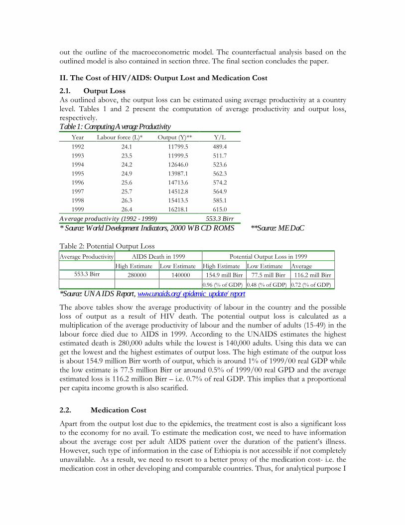
II. The Cost of HIV/AIDS: Output Lost and Medication Cost 2.1. Output Loss As outlined above, the output loss can be estimated using average productivity at a country level. Tables 1 and 2 present the computation of average productivity and output loss, respectively. Table 1: Computing Average Productivity

Year Labour force (L)* Output (Y)** Y/L 1992 24.1 11799.5 489.4 1993 23.5 11999.5 511.7 1994 24.2 12646.0 523.6 1995 24.9 13987.1 562.3 1996 25.6 14713.6 574.2 1997 25.7 14512.8 564.9 1998 26.3 15413.5 585.1 1999 26.4 16218.1 615.0

Average productivity (1992 - 1999) 553.3 Birr * Source: World Development Indicators, 2000 WB CD ROMS **Source: MEDaC Table 2: Potential Output Loss Average Productivity AIDS Death in 1999 Potential Output Loss in 1999 High Estimate Low Estimate High Estimate Low Estimate Average

553.3 Birr 280000 140000 154.9 mill Birr 77.5 mill Birr 116.2 mill Birr 0.96 (% of GDP) 0.48 (% of GDP) 0.72 (% of GDP)*Source: UNAIDS Report, www.unaids.org/epidemic_update/report

The above tables show the average productivity of labour in the country and the possible loss of output as a result of HIV death. The potential output loss is calculated as a multiplication of the average productivity of labour and the number of adults (15-49) in the labour force died due to AIDS in 1999. According to the UNAIDS estimates the highest estimated death is 280,000 adults while the lowest is 140,000 adults. Using this data we can get the lowest and the highest estimates of output loss. The high estimate of the output loss is about 154.9 million Birr worth of output, which is around 1% of 1999/00 real GDP while the low estimate is 77.5 million Birr or around 0.5% of 1999/00 real GPD and the average estimated loss is 116.2 million Birr – i.e. 0.7% of real GDP. This implies that a proportional per capita income growth is also scarified.

2.2. Medication Cost Apart from the output lost due to the epidemics, the treatment cost is also a significant loss to the economy for no avail. To estimate the medication cost, we need to have information about the average cost per adult AIDS patient over the duration of the patient’s illness. However, such type of information in the case of Ethiopia is not accessible if not completely unavailable. As a result, we need to resort to a better proxy of the medication cost- i.e. the medication cost in other developing and comparable countries. Thus, for analytical purpose I

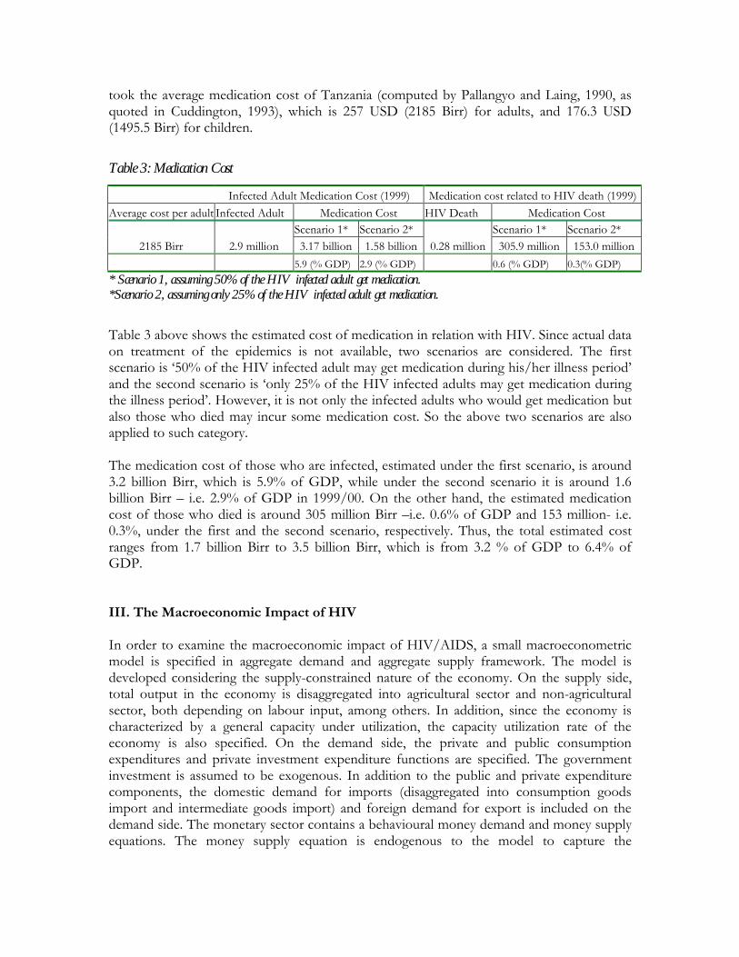
took the average medication cost of Tanzania (computed by Pallangyo and Laing, 1990, as quoted in Cuddington, 1993), which is 257 USD (2185 Birr) for adults, and 176.3 USD (1495.5 Birr) for children.

Table 3: Medication Cost

Infected Adult Medication Cost (1999) Medication cost related to HIV death (1999)Average cost per adult Infected Adult Medication Cost HIV Death Medication Cost Scenario 1* Scenario 2* Scenario 1* Scenario 2*

2185 Birr 2.9 million 3.17 billion 1.58 billion 0.28 million 305.9 million 153.0 million 5.9 (% GDP) 2.9 (% GDP) 0.6 (% GDP) 0.3(% GDP) * Scenario 1, assuming 50% of the HIV infected adult get medication. *Scenario 2, assuming only 25% of the HIV infected adult get medication.

Table 3 above shows the estimated cost of medication in relation with HIV. Since actual data on treatment of the epidemics is not available, two scenarios are considered. The first scenario is ‘50% of the HIV infected adult may get medication during his/her illness period’ and the second scenario is ‘only 25% of the HIV infected adults may get medication during the illness period’. However, it is not only the infected adults who would get medication but also those who died may incur some medication cost. So the above two scenarios are also applied to such category. The medication cost of those who are infected, estimated under the first scenario, is around 3.2 billion Birr, which is 5.9% of GDP, while under the second scenario it is around 1.6 billion Birr – i.e. 2.9% of GDP in 1999/00. On the other hand, the estimated medication cost of those who died is around 305 million Birr –i.e. 0.6% of GDP and 153 million- i.e. 0.3%, under the first and the second scenario, respectively. Thus, the total estimated cost ranges from 1.7 billion Birr to 3.5 billion Birr, which is from 3.2 % of GDP to 6.4% of GDP. III. The Macroeconomic Impact of HIV In order to examine the macroeconomic impact of HIV/AIDS, a small macroeconometric model is specified in aggregate demand and aggregate supply framework. The model is developed considering the supply-constrained nature of the economy. On the supply side, total output in the economy is disaggregated into agricultural sector and non-agricultural sector, both depending on labour input, among others. In addition, since the economy is characterized by a general capacity under utilization, the capacity utilization rate of the economy is also specified. On the demand side, the private and public consumption expenditures and private investment expenditure functions are specified. The government investment is assumed to be exogenous. In addition to the public and private expenditure components, the domestic demand for imports (disaggregated into consumption goods import and intermediate goods import) and foreign demand for export is included on the demand side. The monetary sector contains a behavioural money demand and money supply equations. The money supply equation is endogenous to the model to capture the

monetization of the deficit. The price and the real exchange equations are also specified and hence they are determined endogenously.

3.1. The Model

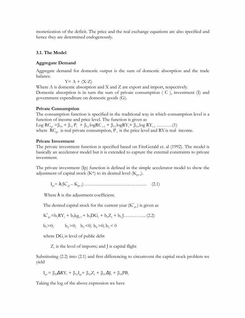
Aggregate Demand Aggregate demand for domestic output is the sum of domestic absorption and the trade balance. Y= A + (X-Z) Where A is domestic absorption and X and Z are export and import, respectively. Domestic absorption is in turn the sum of private consumption ( C ), investment (I) and government expenditure on domestic goods (G). Private Consumption The consumption function is specified in the traditional way in which consumption level is a function of income and price level. The function is given as Log RCpt =β10 + β11 Pt + β12 logRC t-1 + β13 logRYt+ β14 log RYt-1

……….(1) where RCpt is real private consumption, P t is the price level and RY is real income. Private Investment The private investment function is specified based on FitzGerald et. al (1992). The model is basically an accelerator model but it is extended to capture the external constraints to private investment.

The private investment (Ip) function is defined in the simple accelerator model to show the adjustment of capital stock (K*) to its desired level (Kpt-1).

Ipt= λ(K*pt – Kpt-1) ………………………………… (2.1)

Where λ is the adjustment coefficient.

The desired capital stock for the current year (K*pt ) is given as

K*pt =b1RYt + b2kgt-1 + b3DGt + b4Zt + b5 J………….. (2.2)

b1>0; b2 >0; b3 <0; b4 >0; b5 < 0

where DGt is level of public debt

Zt is the level of imports; and J is capital flight

Substituting (2.2) into (2.1) and first differencing to circumvent the capital stock problem we yield

Ipt = β20∆RYt + β21Igt+ β22Zt + β23 ∆Jt + β24PBt

Taking the log of the above expression we have

LogIpt = β20∆LogRYt + β21 LogIgt+ β22 LogZt + β23 ∆LogJt + β24 LogPBt ……….(2.3)

Where PB is first difference of DG and implies public current borrowing; and Igt is the first difference of government capital stock implying the government investment expenditure. Since the measurement of capital flight is controversial and may not also be important factor in Ethiopian context, ∆J will not be used in the estimation process.

Government Sector

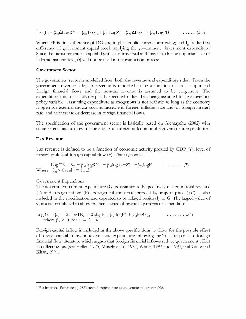
The government sector is modelled from both the revenue and expenditure sides. From the government revenue side, tax revenue is modelled to be a function of total output and foreign financial flows and the non-tax revenue is assumed to be exogenous. The expenditure function is also explicitly specified rather than being assumed to be exogenous policy variable1. Assuming expenditure as exogenous is not realistic so long as the economy is open for external shocks such as increase in foreign inflation rate and/or foreign interest rate, and an increase or decrease in foreign financial flows.

The specification of the government sector is basically based on Alemayehu (2002) with some extensions to allow for the effects of foreign inflation on the government expenditure.

Tax Revenue

Tax revenue is defined to be a function of economic activity proxied by GDP (Y), level of foreign trade and foreign capital flow (F). This is given as

Log TR = β30 + β31 logRY t + β32log (x+Z) +β33 logF t ………………(3)

Where β3i > 0 and i = 1…3 Government Expenditure The government current expenditure (G) is assumed to be positively related to total revenue (T) and foreign inflow (F). Foreign inflation rate proxied by import price ( pm) is also included in the specification and expected to be related positively to G. The lagged value of G is also introduced to show the persistence of previous patterns of expenditure Log Gt = β50 + β51 logTRt + β52logF t + β53 logPm + β54logG t-1 …………..(4)

where β5i > 0 for i = 1…4

Foreign capital inflow is included in the above specifications to allow for the possible effect of foreign capital inflow on revenue and expenditure following the 'fiscal response to foreign financial flow' literature which argues that foreign financial inflows reduce government effort in collecting tax (see Heller, 1975, Mosely et. al, 1987, White, 1993 and 1994, and Gang and Khan, 1991).

1 For instance, Feltensten (1985) treated expenditure as exogenous policy variable.

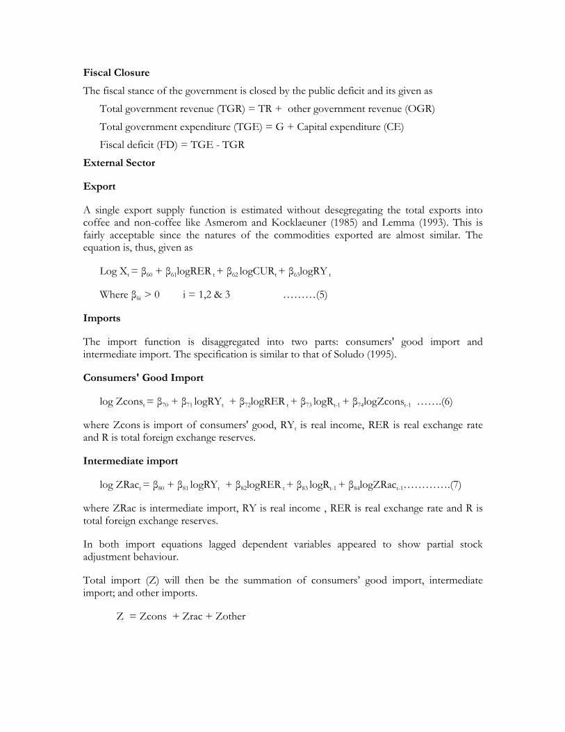
Fiscal Closure

The fiscal stance of the government is closed by the public deficit and its given as

Total government revenue (TGR) = TR + other government revenue (OGR)

Total government expenditure (TGE) = G + Capital expenditure (CE)

Fiscal deficit (FD) = TGE - TGR

External Sector

Export

A single export supply function is estimated without desegregating the total exports into coffee and non-coffee like Asmerom and Kocklaeuner (1985) and Lemma (1993). This is fairly acceptable since the natures of the commodities exported are almost similar. The equation is, thus, given as

Log Xt = β60 + β61logRER t + β62 logCURt + β63logRY t

Where β6i > 0 i = 1,2 & 3 ………(5)

Imports

The import function is disaggregated into two parts: consumers' good import and intermediate import. The specification is similar to that of Soludo (1995).

Consumers' Good Import

log Zconst = β70 + β71 logRYt + β72logRER t + β73 logRt-1 + β74logZconst-1 …….(6)

where Zcons is import of consumers' good, RYt is real income, RER is real exchange rate and R is total foreign exchange reserves.

Intermediate import

log ZRact = β80 + β81 logRYt + β82logRER t + β83 logRt-1 + β84logZRact-1………….(7)

where ZRac is intermediate import, RY is real income , RER is real exchange rate and R is total foreign exchange reserves.

In both import equations lagged dependent variables appeared to show partial stock adjustment behaviour.

Total import (Z) will then be the summation of consumers’ good import, intermediate import; and other imports.

Z = Zcons + Zrac + Zother

External Sector Closure

The external sector is closed by the reserve flows identity in which the accumulation or de-accumulation of reserves take place. Except the trade balance, the other components of the external sector are exogenous in the model

BOP = CA + Transfer payments + capital account balance + net errors and omissions

Change in Reserve = BOP + change in arrears + debt relief

Reserve (t) = Reserve (t-1) + Change in reserve (t)

Where CA (current account) is given as the sum of trade balance + net services + net private transfer payments.

Aggregate Supply

Production

In modelling the production side, the production sectors are disaggregated into agricultural and non-agricultural. The agricultural and the non-agricultural production functions are distinguished and specified on the basis of the economic structure of the country.

Agricultural Production Function The agricultural production function is assumed to be positively related with labour in the agricultural sector, rainfall, and relative price of agricultural products. The function is given as:

Log Yagr = β90 + β91 logLagrt + β92logRFt-1 + β93 log(nagr

agr

PP

)t + β94logYagrt-1 ..…(8)

Where Yagr is agricultural GDP, Lagr is labour force in agricultural sector, RF is rainfall, and Pagr/Pnagr is the ratio of agricultural GDP deflator to non agricultural GDP deflator. The data for labour force is adjusted using the capacity utilization rate in the agricultural sector to proxy employed labour force in the sector since the data for employed labour force is not available.

Non-Agricultural Production Function

The non-agricultural sector contains both manufacturing and service sectors. The non-agricultural production sector is determined by labour force in the sector, change in capital stock, intermediate import and capacity utilization in the economy. This production function is given as

Log Ynagr = β100 + β101 log Lnagrt+β102 log∆Kt+β103logZract + β104 logCUR ………..(9)

Where Lnagr is labour force in non-agricultural sector, ∆Kt is change in capital stock, Zrac is intermediate imports, and CUR is capacity utilization rate in the economy. The data for

labour force is adjusted using the capacity utilization rate in the non-agricultural sector since the data for employed labour force is not readily available.

The total production will be given as

RY= Yagr + Ynagr

Capacity Utilization Rate

Capacity under utilization in the economy may come from both the agricultural sector and the non-agricultural sector. Under utilization of capacity in the agricultural sector can be mainly attributed to shortage of rainfall, among other things. In the non-agricultural sector the main cause of under utilization of capacity is shortage of imported inputs. Thus, capacity utilization in the economy is assumed to be dependent on the level of capital imports, total export earnings and rainfall.

Log CURt = β110 + β111logRFt-1 +β112logZcap …………………..(10)

β i >0 where i = 1 & 2; RF is rain fall and Zcap is intermediate imports. Prices The domestic price level is expected to be determined by the excess demand over the supply in the domestic economy (RED) excess money supply over the money demand (EMs) and import prices (Pm). In addition to this, capacity utilization rate (CUR) is also related with the rate of inflation because it shows the nature of mark-up pricing. The mark-up (the profit margin) is assumed to be an increasing function of the capacity utilization rate (Soludo, 1995). Thus, the inflation equation is given as

Pt = β120 + β121 EMs + β122log REDt + β123 logCURt + β124logPm………………………(11)

Money Market

Money Supply

The money supply equation is specified in such a way that it is partly endogenous from the side of the balance of payments and the fiscal deficit. Following the flow of funds approach, the domestic money supply (Ms) in the economy can be given as

Ms = (TGR-TGE) - Gsp + DCp + ∆R …………..(12)

Where (TGR – TGE) is the budget deficit, Gsp is net sales of government interest bearing

assets to the non-bank private sector, DCp is domestic credit to the private sector, ∆F is change in foreign financial flows, and ∆R is change in foreign exchange reserve.

Money Demand

The demand for real money balance (M/P) is positively related to income (RY) and negatively related with the opportunity cost of holding money. The demand for the real money is given as:

Log (M/P)t = β140 + β141 logRY t - β142rt + β143 π t + β144log(M /P )t-1………(13)

Where r and π are interest rate and inflation rate, respectively. And they are used to proxy opportunity cost of holding money. Exchange Rate Since the nominal exchange rate had been fixed for long period of time, the specification of the exchange rate will be based on the real exchange rate. The real exchange rate equation follows similar formulation as that of Ghura and Grennes (1993).

Log RER = β150 + β151 logTOT t - β152log(OPEN)t + β153 logFt + β154 EMs ………(14)

Where RER is the real exchange rate, TOT is terms of trade,

OPEN = [(X+Z)/ Y] is the ratio of GDP over the sum of imports (Z) and exports (X); F is foreign financial flows, and EMs is excess money supply, measured as the difference between money supply and money demand.

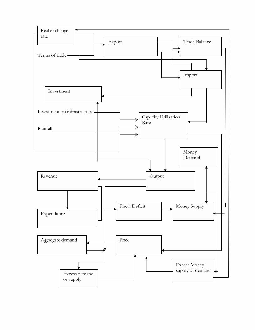
3.2. The Working of the Model

The operation of the model is as follows (also see the chart below). The value of export together with foreign financial inflows (i.e. foreign exchange availability), terms of trade and real exchange rate determine the level of imports. Imports, in turn, affect the level of private investment and determine the capacity utilization rate of the economy along with the exogenously given weather condition and availability of infrastructure. The capacity utilization rate is assumed to have a direct impact on output which in turn affects government revenue and expenditure and hence the fiscal deficit. The fiscal deficit has a feed back effect on prices through its effect on money supply. The level of output also determined the aggregate demand. The excess demand over the total output is assumed to be financed by foreign financial flows. However, for a given level of foreign financial flows, the disequilibrium between aggregate demand and aggregate supply is assumed to spillover to the domestic price (note that the price equation includes excess demand as an argument) and market clearing will be achieved through adjustment in price.

3.3. Estimation Techniques

The individual equations in the model are estimated in an ECM format using the Johansen approach in view of the time series properties of the macro-time series variables for the period of 1965/66 – 1998/99 (see the appendix for the complete result of the estimated equations). The model has 30 equations of which 14 are behavioural and 16 are identities and technical relationships. The scenario that will be experimented is that what would have been the performance of the economy, had there been a 10% decline in the labour force since 1980/81 due to HIV. The scenario experimented hear is that what would have been the performance of the economy, had there been a 10% decline in the labour force since 1980/81 due to HIV. Thus, the result should be interpreted carefully with these caveats in mind.

Terms of trade Investment on infrastructure Rainfall

Export

Import

Capacity Utilization Rate

OutputRevenue

Expenditure Fiscal Deficit Money Supply

Trade Balance

PriceAggregate demand

Excess demand or supply

Investment

Money Demand

Real exchange rate

Excess Money supply or demand

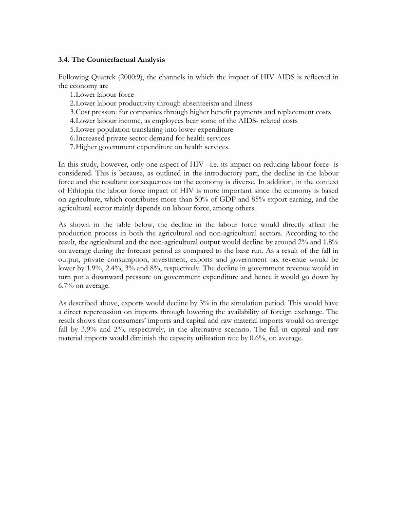
3.4. The Counterfactual Analysis Following Quattek (2000:9), the channels in which the impact of HIV AIDS is reflected in the economy are

1. Lower labour force 2. Lower labour productivity through absenteeism and illness 3. Cost pressure for companies through higher benefit payments and replacement costs 4. Lower labour income, as employees bear some of the AIDS- related costs 5. Lower population translating into lower expenditure 6. Increased private sector demand for health services 7. Higher government expenditure on health services.

In this study, however, only one aspect of HIV –i.e. its impact on reducing labour force- is considered. This is because, as outlined in the introductory part, the decline in the labour force and the resultant consequences on the economy is diverse. In addition, in the context of Ethiopia the labour force impact of HIV is more important since the economy is based on agriculture, which contributes more than 50% of GDP and 85% export earning, and the agricultural sector mainly depends on labour force, among others.

As shown in the table below, the decline in the labour force would directly affect the production process in both the agricultural and non-agricultural sectors. According to the result, the agricultural and the non-agricultural output would decline by around 2% and 1.8% on average during the forecast period as compared to the base run. As a result of the fall in output, private consumption, investment, exports and government tax revenue would be lower by 1.9%, 2.4%, 3% and 8%, respectively. The decline in government revenue would in turn put a downward pressure on government expenditure and hence it would go down by 6.7% on average. As described above, exports would decline by 3% in the simulation period. This would have a direct repercussion on imports through lowering the availability of foreign exchange. The result shows that consumers’ imports and capital and raw material imports would on average fall by 3.9% and 2%, respectively, in the alternative scenario. The fall in capital and raw material imports would diminish the capacity utilization rate by 0.6%, on average.

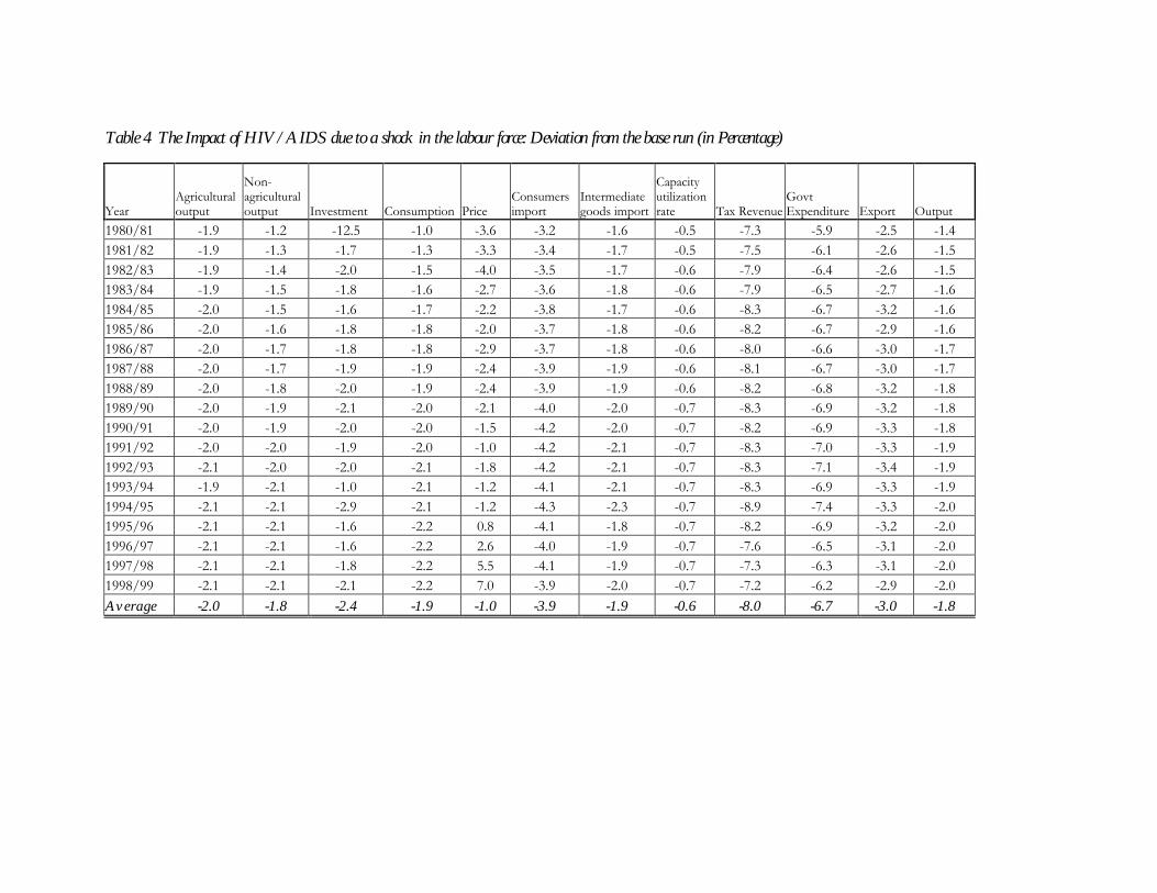
Table 4 The Impact of HIV/AIDS due to a shock in the labour force: Deviation from the base run (in Percentage)

Year Agricultural output

Non-agricultural output Investment Consumption Price

Consumers import

Intermediate goods import

Capacity utilization rate Tax Revenue

Govt Expenditure Export Output

1980/81 -1.9 -1.2 -12.5 -1.0 -3.6 -3.2 -1.6 -0.5 -7.3 -5.9 -2.5 -1.4 1981/82 -1.9 -1.3 -1.7 -1.3 -3.3 -3.4 -1.7 -0.5 -7.5 -6.1 -2.6 -1.5 1982/83 -1.9 -1.4 -2.0 -1.5 -4.0 -3.5 -1.7 -0.6 -7.9 -6.4 -2.6 -1.5 1983/84 -1.9 -1.5 -1.8 -1.6 -2.7 -3.6 -1.8 -0.6 -7.9 -6.5 -2.7 -1.6 1984/85 -2.0 -1.5 -1.6 -1.7 -2.2 -3.8 -1.7 -0.6 -8.3 -6.7 -3.2 -1.6 1985/86 -2.0 -1.6 -1.8 -1.8 -2.0 -3.7 -1.8 -0.6 -8.2 -6.7 -2.9 -1.6 1986/87 -2.0 -1.7 -1.8 -1.8 -2.9 -3.7 -1.8 -0.6 -8.0 -6.6 -3.0 -1.7 1987/88 -2.0 -1.7 -1.9 -1.9 -2.4 -3.9 -1.9 -0.6 -8.1 -6.7 -3.0 -1.7 1988/89 -2.0 -1.8 -2.0 -1.9 -2.4 -3.9 -1.9 -0.6 -8.2 -6.8 -3.2 -1.8 1989/90 -2.0 -1.9 -2.1 -2.0 -2.1 -4.0 -2.0 -0.7 -8.3 -6.9 -3.2 -1.8 1990/91 -2.0 -1.9 -2.0 -2.0 -1.5 -4.2 -2.0 -0.7 -8.2 -6.9 -3.3 -1.8 1991/92 -2.0 -2.0 -1.9 -2.0 -1.0 -4.2 -2.1 -0.7 -8.3 -7.0 -3.3 -1.9 1992/93 -2.1 -2.0 -2.0 -2.1 -1.8 -4.2 -2.1 -0.7 -8.3 -7.1 -3.4 -1.9 1993/94 -1.9 -2.1 -1.0 -2.1 -1.2 -4.1 -2.1 -0.7 -8.3 -6.9 -3.3 -1.9 1994/95 -2.1 -2.1 -2.9 -2.1 -1.2 -4.3 -2.3 -0.7 -8.9 -7.4 -3.3 -2.0 1995/96 -2.1 -2.1 -1.6 -2.2 0.8 -4.1 -1.8 -0.7 -8.2 -6.9 -3.2 -2.0 1996/97 -2.1 -2.1 -1.6 -2.2 2.6 -4.0 -1.9 -0.7 -7.6 -6.5 -3.1 -2.0 1997/98 -2.1 -2.1 -1.8 -2.2 5.5 -4.1 -1.9 -0.7 -7.3 -6.3 -3.1 -2.0 1998/99 -2.1 -2.1 -2.1 -2.2 7.0 -3.9 -2.0 -0.7 -7.2 -6.2 -2.9 -2.0 Average -2.0 -1.8 -2.4 -1.9 -1.0 -3.9 -1.9 -0.6 -8.0 -6.7 -3.0 -1.8

IV. Conclusion

HIV/AIDS has a diverse impact in the economy as it affects the labour force and hence output, government expenditure and revenue apart from the social chaos that it creates. In this study, attempt is made to quantify the economic impact of HIV in the Ethiopian economy. To do so, three approaches are used. The first one is to use the direct method of average productivity to estimate output lost. The second one is to estimate medication cost using average cost per AIDS patient. The third one is a counterfactual simulation analysis using a macroeconometric method.

The result shows that output loss to be in the range of 0.5% to 1% while the medication cost ranges from 3.2% to 6.4% of GDP in 1999/00. From the counterfactual analysis it can be discerned that the prevalence of HIV/AIDS has a negative impact on the overall economy through lowering the active labour force. The decline in the labour force has a direct negative impact on both the output of the agricultural and non-agricultural sectors that would lead to the fall in private consumption, investment, exports and government tax revenue. The slow down of the economy would also be strengthened with the fall in imports due to the decline in exports and hence the shrinking down of the importing capacity.

Reference:

Agénore, P.R. And Montiel, P.J. (1996) Development Macroeconomics, Princeton and New Jersey: Princeton University Press.

Aghevli, B. And Sassanpour,, C. (1991). “Prices, Output, and Trade Balance in Iran” , In Khan, M., Montiel, P., and Haque, N. (Ed). Macroeconomic Models For Adjustment in Developing Countries. Washington D.C.: IMF.

Alemayehu Geda (1997) “The Historical Origin of African Debt and Financial Crisis,” Institute of Social Studies Working Paper Series on Money, Finance and Development, 62. The Hague: Institute of Social Studies.

Alemayehu Geda (2002) Finance and Trade in Africa: Macroeconomic Response in a World Economy Context, London: Pallgrave-Macmillan

Alemayehu Geda (1999a) "Projection of Major Macro Aggregates of Ethiopia,” Background Paper for Ethiopian Economic Association- ‘The Ethiopian Economy Project’ Addis Ababa.

Alemayehu Geda (1999b) “The Structure and Performance of Ethiopia’s Financial Sector in The Pre and Post Reform Period: With Special Focus on Banking,” In the Ethiopian Economy Performance and Evaluation, (Alemayehu Geda and Berhanu Nega, Ed.) Addis Ababa.

Alemayehu Geda (1999c) “Profile of Ethiopia’s External Trade,” In the Ethiopian Economy Performance and Evaluation, (Alemayehu Geda And Berhanu Nega, Ed.) Addis Ababa.

Alemayehu Geda. (2000) “Macroeconomic Performance in Post-Reform Ethiopia,” A Paper Presented at Symposium on the Performance of the Ethiopian Economy in the Post-Derg Period, April 26, 2000, Addis Ababa.

Alemayehu Geda and Daniel Zerfu (1999) “Profile of Ethiopia’s External Debt”, In the Ethiopian Economy Performance and Evaluation, (Alemayehu Geda and Berhanu Nega, Ed) Addis Ababa.

Asemerom Kidane and Kocklaeuner (1985). “A Macroeconometric Model for Ethiopia: Specification, Estimation and Forecast and Control”, East African Economic Review,

Assefa Sumoro (2000) “Saving Mobilization In Ethiopia,” Economic and Market Research Unit, Commercial Bank of Ethiopia. (Unpublished)

Backhouse, R.. (1995) Interpreting Macroeconomics: Explorations in the History of Macroeconomic Thought, London: Routledge.

Bethelemy J. And Söderling L (2001) “Will There Be New Emerging Countries in Africa by the Year 2020?” www.oecd.org/dev

Bodart, V. And Le Dem, J. (1996) “Labour Market Representation in Quantitative Macroeconomic Models for Developing Countries: An Application to Côte d’Ivoire,” IMF Staff Papers 43:2, 419 – 451.

Branson, W. (1989) Macroeconomic Theory and Policy, 3rd ed., Harper and Row, Publishers, New York.

Challen, D.W And Hagger, A.J (1983) Macroeconometric Systems: Construction, Validation and Applications, London: Macmillan Press.

Chishti, S., Hasan, M. And Mahmud, S. (1992) “Macroeconometric Modelling and Pakistan’s Economy: A Vector Autoregression Approach,” Journal of Development Economics 38, 353 – 370.

Daniel Zerfu (1998) The Fiscal Response to External Financial Flows in Ethiopia, Unpublished BA Thesis, Department of Economics, Addis Ababa University.

Daniel Zerfu (2001 a) “Macroeconometric Policy Modeling for Ethiopia,” Unpublished MSc. Thesis, Department of Economics, Addis Ababa University

Davies, R., Rattsø, J. And Torvik, R. (1994) “The Macroeconomics of Zimbabwe in the 1980s: A CGE Model Analysis,” Journal of African Economies, 3:2, 153- 198.

Decaluwé, B. And Nsengiyumva, F. (1994) “Policy Impact Under Credit Rationing: A Real and Financial CGE Model of Rwanda,” Journal of African Economies, 3:2, 262-308.

Doornik, J. And Hendry, D. (1997) Modelling Dynamic Systems Using Pc Fiml 9.0 for Windows, London: International Thomson Business Press.

Egawaikhide, F. (1997) “Effects of Budget Deficits on the Current Account Balance in Nigeria: A Simulation Exercise,” AERC Research Paper, 70.

Elbadawi, I. And Schmidt-Hebbel, K. (1991) “Macroeconomic Structure and Policy in Zimbabwe: Analysis and Empirical Model, 1965 –88,” World Bank Working Papers, 772, Washington, D.C.: World Bank.

El-Shekh, S. (1992) “Towards a Macroeconometric Policy Model of a Semi-Industrial Economy: The Case of Egypt,” Economic Modelling, 9:1, 75 –95.

Enders, W. (1995) Using Cointegration Analysis in Econometric Modelling, London: Harvester Wheatsheaf.

Fair R.C. (1993) "Estimating Event Probabilities from Macroeconometric Models Using Simulation," In Business Cycle, Indicators and Forecasting, (Stock And M.W. Watson, Ed). NEBR Studies in Business Cycles : 28. Chicago: University Of Chicago Press.

Fair R.C. (1994), Testing Macroeconometric Models. London: Harvard University Press. Feltenstein, A. (1985). “Stabilization of the Balance of Payments in a Small Planned Economy,

With an Application to Ethiopia,” Journal of Development Economics, 18:171-191. Fitzgerald, E.V.K., K. Jansen and R. Vos (1992). “Externally Constraints on Private

Investment Decisions in Developing Countries”, ISS Working Paper, Sub-Series on Money, Finance and Development: 43, The Hague: Institute of Social Studies.

Frenkel, J. (1991) “Foreword” In Macroeconomic Models for Adjustment in Developing Countries (Khan, M., Montiel, P.J. And Haque, N., Ed) Washington D.C.: IMF.

Frenkel, J. and H. Johnson (1976) The Monetary Approach to the Balance of Payments, London: Alen and Unwin.

Gang, I. and H. Khan (1991) “Foreign Aid, Taxes and Public Investment,” Journal of Development Economics, 34:355-369.

Garrat, A., K. Lee, H. Pesaran and Y. Shin (1999) “A Structural Cointegrating VAR Approach to Macroeconometric Modelling,” www.econ.cam.ac.uk/faculty/pesaran/ni99.pdf

Ghura,D. and T. Grennes (1993) "The Real Exchange Rate and Macroeconomic Performance in Sub-Saharan Africa" Journal of Development Economics, 42:1.

Go, D.S. (1994) “External Shocks, Adjustment Policies And Investment in a Developing Economy: Illustration from a Forward Looking CGE Model of the Philippines,” Journal of Development Economics 44:2, 229-262.

Haque, N.U., K. Lahiri, and P.J. Montiel (1991). “A Macroeconomic Model for Developing Countries,” In Macroeconomic Models for Adjustment in Developing Countries (.Khan, M., Montiel, P., And Haque, N., Ed ). Washington D.C.: IMF.

Harris, J. (1985) “A Survey of Macroeconomic Modelling in Africa,” Paper Presented to the Eastern and Southern Africa Macroeconomic Research Network, December 7- 13, Nairobi, Kenya.

Heller, P.S. (1975). “A Model of Public Fiscal Behavior in Developing Countries: Aid, Investment and Taxation”, The American Economic Revenue, 65(3): 429-445.

Horton, S. and J. Mclaren (1989) “Supply Constraints in the Tanzanian Economy: Simulation Results from a Macroeconometric Model,” Journal of Policy Modelling 11:2, 297 – 313.

Ioyoha, M. (1996) “Macroeconometric Models,” In Macroeconomic Policy Analysis: Tools, Techniques and Applications to Nigeria (Obadan, M And Ioyaha, M. , Ed) Ibadan, Nigeria.

Johansen, S. (1988). “Statistical Analysis of Cointegration Vectors”, Journal of Economic Dynamics and Control, 12: 231-254.

Johansen, S., (1996) Likelihood-Based Inference in Cointegrating Vector Auteregressive Models, New York: Oxford University Press.

Khan, M., P. Montiel and N. Haque, Ed. (1991). Macroeconomic Models for Adjustment in Developing Countries. Washington D.C.: IMF

Kouassi, E. (1997) “A Macroeconometric Model for Côte d’Ivoire,” Unpublished paper, AERC

Lemma Mered (1993). “Modelling the Ethiopian Economy: Experience and Prospects” (Memo).

Lipumba, N., B. Ndulu, S. Horton and A. Plourde (1988) “A Supply Constrained Macro-Econometric Mode of Tanzania,” Economic Modelling. 5(4): 354-380

Lucas, R.E. (1976), "Economic Policy Evaluation: A Critique, The Phillips Curve and Labour Markets,” Caneige Rocheeler Series on Public Policy: 1, 19 - 46., ( K. Brunner and A.H. Meltzer, Ed.).

Lucas, R.E. and T.J. Sargent (1978). “After Keynesian Macroeconomics”, In After Phillips Curve: Persistence of High Inflation and High Unemployment. Conference Series No. 19, Federal Reserve Bank of Boston, 44-72.

Masson, P., S. Symansky and G. Meredith (1990) “Multimod Mark II: A Revised and Extended Model,” IMF Occasional Paper, 71, Washington, D.C.: IMF.

Mosley, P., J. Hudson and S. Horrell, (1987). “Aid, the Public Sector and the Market in Less Developed Countries”, The Economic Journal, 97(181):616-641.

Mukherjee, C., H. White and M. Wuyts (1998) Econometrics and Data Analysis for Developing Countries, London: Routledge.

Murinde, V. (1993) Macroeconomic Policy Modelling for Developing Countries, London: Avebury.

Murphy, C.W., I.A. Bright,. R.J. Brooker, W.D. Geeves, and B.K. Taplin, (1986). “A Macroeconometric Model of the Australian Economy for Medium Term Policy Analysis”, Technical Paper: 2 Commonwealth of Australia, Economic Planning Advisory Council.

Ndulu, B.J (1991) “Growth and Adjustment in Sub-Saharan Africa,” in Economic Reform in Sub-Saharan Africa (Chhibber, A. and Fisher, S., Editors) Washington D.C.: The World Bank.

Oshikoya, T.W. (1990) The Nigerian Economy: A Macroeconometric and Input-Output Model, New York: PRAEGER.

Pagan, A. (1987) “Three Econometric Methodologies: A Critical Appraisal,” Journal of Economic Surveys 1, 3-24.

Perera, N. (1994) “Exogenous Shocks and Macroeconomic Policies in LDCs: A Study of Sri Lanka with an Econometric Model,” Journal of Policy Modelling 16:3, 335-344.

Pilbeam, K. (1998) International Finance 2nd Ed, London: Macmillan.

Polak, J.J. (1957) “Monetary Analysis of Income Formation and Payments Problems,” IMF Staff Papers 6 , 1-50.

Quattek, K. (2000) “Economic Impact of AIDS in South Africa,” www.ingbarings.com

Rattsø, J. (1994) “Medium –run Adjustment under Import Compression: Macroeconomic Analysis Relevant for Sub-Saharan Africa,” Journal of Development Economics, 45: 35 – 54.

Robinson, S and D. Roland-Holst (1988) “Macroeconomic Structure and Computable General Equilibrium Models,” Journal of Policy Modelling, 10:3, 353 – 375.

Robinson, S. (1989) “Multisectoral Models,” In Handbook of Development Economics, 2, 85-945 (Chenery, H And Srinivasan, T.N., Ed) Amsterdam: North Holland.

Salvatore, D. (1989) “The Prototype Model,” In African Development Prospects: A Policy Modelling Approach (Salvatore, D., Ed.) New York: Taylor and Francis.

Sargan, J.D (1964) “Wages and Prices in The United Kingdom: A Study in Econometric Methodology,” In Econometric Analysis of National Economic Planning, 16, 25- 63 (Hart, P.E, Mills, G. And Whitaker, J.K, Ed) London.

Seid Nuru. (2000) Determinants of Economic Growth in Ethiopia, Unpublished Msc. Thesis, Department of Economics, Addis Ababa University.

Sims, C. (1980) “Macroeconomics and Reality,” Econometrica, 48, 1- 48. Soludo, C. (1995) "Macroeconomic Adjustment, Trade and Growth: Policy Analysis Using a

Macroeconomic Model of Nigeria" AERC Research Paper:32. Storm, S. (1994) “The Macroeconomic Impact of Agricultural Policy: A CGE Analysis for

India,” Journal of Policy Modelling 16:1, 55 - 96. Taylor, L. (1983) Structuralist Macroeconomics: Applicable Models for The Third World, New York:

Basic Books.

Taylor, L. (1990) “Structuralist CGE Models,” In Structuralist Computable General Equilibrium Models: Socially Relevant Policy Analysis for the Developing World (Taylor, L., Ed.) Cambridge: MIT Press.

Taylor, L. (1991) Income Distribution, Inflation and Growth: Lectures on Structuralist Macroeconomic Theory. Cambridge, Ms: The MIT Press.

UNAIDS (2000) UNAIDS Report 2000, www.unaids.org/epidemic_update/report

Van Frausum, Y. and Sahn, D.E (1993) “An Econometric Model for Malawi: Measuring the Effects of External Shock and Policies,” Journal of Policy Modelling 15:3, 313-327.

Wallis, K. (1995) "Large Scale Macroeconometric Modelling," In Handbook of Applied Econometrics: Macroeconmics (Pesaran, M.H. and Wickens, M.,Ed) UK: Blackwell Publishers,

Wallis, K, and J. Whitley (1987) "Long Run Properties of Large Scale Macroeconometric Models," Annales d'Economie Et De Statistique, 207-24.

Wallis, K., and J. Whitley (1991) "Large Scale Econometric Models of National Economies: Part I, Some Current Developments," Scandinavian Journal of Economics, 93:2, 283-296.

Wallis, K.F (1989) “Macroeconomic Forecasting: A Survey,” Economic Journal 99, 28-61. White, H. (1993) “Aid and Government: A Dynamic Model of Aid, Income and Fiscal

Behaviour”, Journal of International Development, 5:3, 305-312. White, H. (1994) “Foreign Aid, Taxes and Public Investment: A Further Comment”, Journal of

Development Economics, 45:155-163.

Whiteman, M.V.N. (1975) “Global Monetarism and the Monetary Approach to the Balance of Payments,” Brookings Papers on Economic Activity 2, 491 – 536.

World Bank (2000) World Development Indicators, 2000, CD ROMS, Washington DC.: World Bank.

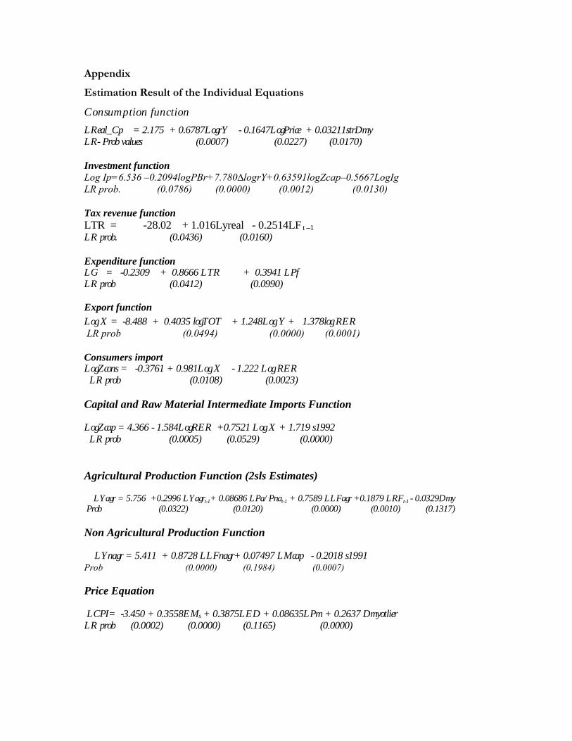
Appendix Estimation Result of the Individual Equations

Consumption function LReal_Cp = 2.175 + 0.6787LogrY - 0.1647LogPrice + 0.03211strDmy LR- Prob values (0.0007) (0.0227) (0.0170) Investment function Log Ip=6.536 –0.2094logPBr+7.780∆logrY+0.63591logZcap–0.5667LogIg LR prob. (0.0786) (0.0000) (0.0012) (0.0130) Tax revenue function LTR = -28.02 + 1.016Lyreal - 0.2514LF t –1 LR prob. (0.0436) (0.0160) Expenditure function LG = -0.2309 + 0.8666 LTR + 0.3941 LPf LR prob (0.0412) (0.0990)

Export function Log X = -8.488 + 0.4035 logTOT + 1.248Log Y + 1.378log RER LR prob (0.0494) (0.0000) (0.0001) Consumers import LogZcons = -0.3761 + 0.981Log X - 1.222 Log RER

LR prob (0.0108) (0.0023) Capital and Raw Material Intermediate Imports Function

LogZcap = 4.366 - 1.584LogRER +0.7521 Log X + 1.719 s1992 LR prob (0.0005) (0.0529) (0.0000)

Agricultural Production Function (2sls Estimates)

LYagr = 5.756 +0.2996 LYagrt-1+ 0.08686 LPa/Pnat-1 + 0.7589 LLFagr +0.1879 LRFt-1 - 0.0329Dmy Prob (0.0322) (0.0120) (0.0000) (0.0010) (0.1317)

Non Agricultural Production Function

LYnagr = 5.411 + 0.8728 LLFnagr+ 0.07497 LMcap - 0.2018 s1991 Prob (0.0000) (0.1984) (0.0007)

Price Equation

LCPI= -3.450 + 0.3558EMs + 0.3875LED + 0.08635LPm + 0.2637 Dmyotlier LR prob (0.0002) (0.0000) (0.1165) (0.0000)

Capacity utilization rate equation

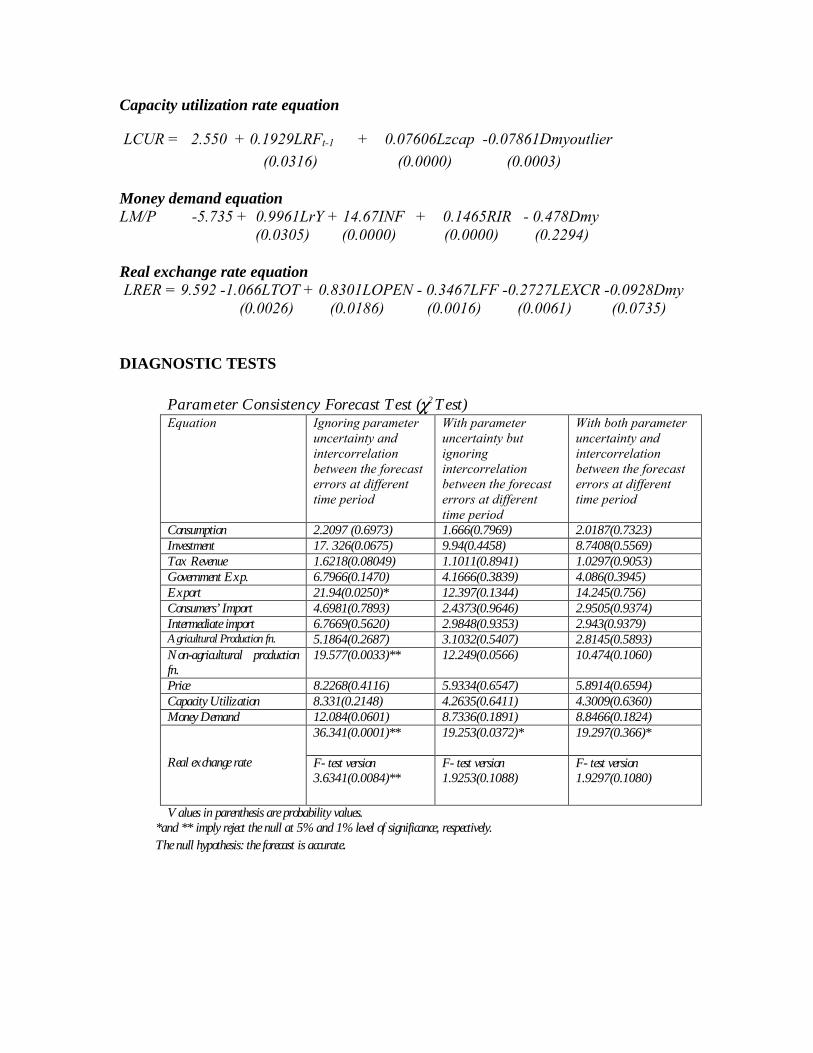
LCUR = 2.550 + 0.1929LRFt-1 + 0.07606Lzcap -0.07861Dmyoutlier (0.0316) (0.0000) (0.0003)

Money demand equation LM/P -5.735 + 0.9961LrY + 14.67INF + 0.1465RIR - 0.478Dmy (0.0305) (0.0000) (0.0000) (0.2294) Real exchange rate equation LRER = 9.592 -1.066LTOT + 0.8301LOPEN - 0.3467LFF -0.2727LEXCR -0.0928Dmy (0.0026) (0.0186) (0.0016) (0.0061) (0.0735) DIAGNOSTIC TESTS

Parameter Consistency Forecast Test (χ2 Test) Equation Ignoring parameter

uncertainty and intercorrelation between the forecast errors at different time period

With parameter uncertainty but ignoring intercorrelation between the forecast errors at different time period

With both parameter uncertainty and intercorrelation between the forecast errors at different time period

Consumption 2.2097 (0.6973) 1.666(0.7969) 2.0187(0.7323) Investment 17. 326(0.0675) 9.94(0.4458) 8.7408(0.5569) Tax Revenue 1.6218(0.08049) 1.1011(0.8941) 1.0297(0.9053) Government Exp. 6.7966(0.1470) 4.1666(0.3839) 4.086(0.3945) Export 21.94(0.0250)* 12.397(0.1344) 14.245(0.756) Consumers’ Import 4.6981(0.7893) 2.4373(0.9646) 2.9505(0.9374) Intermediate import 6.7669(0.5620) 2.9848(0.9353) 2.943(0.9379) Agricultural Production fn. 5.1864(0.2687) 3.1032(0.5407) 2.8145(0.5893) Non-agricultural production fn.

19.577(0.0033)** 12.249(0.0566) 10.474(0.1060)

Price 8.2268(0.4116) 5.9334(0.6547) 5.8914(0.6594) Capacity Utilization 8.331(0.2148) 4.2635(0.6411) 4.3009(0.6360) Money Demand 12.084(0.0601) 8.7336(0.1891) 8.8466(0.1824)

36.341(0.0001)**

19.253(0.0372)* 19.297(0.366)* Real exchange rate F- test version

3.6341(0.0084)** F- test version 1.9253(0.1088)

F- test version 1.9297(0.1080)

Values in parenthesis are probability values. *and ** imply reject the null at 5% and 1% level of significance, respectively. The null hypothesis: the forecast is accurate.