Embed Size (px)
Citation preview

The Lorenz Model of the Size Distribution of Income
B. EssamaB. Essama--NssahNssahPoverty Reduction GroupPoverty Reduction Group
(PRMPR)(PRMPR)The World Bank
October 17, 2005Module 3

2
Foreword“The effect of ignoring the
interpersonal variations can, in fact, be deeply inegalitarian, in hiding the fact that equal consideration for all may demand very unequal treatment in favour of the disadvantaged.”
Sen (1992)

3
OutlineOutline1. The Lorenz Curve
StructureNormative UnderpinningsParameterization
2. Recovering the Size Distribution and Associated Measures of Inequality and Poverty
StrategyThe Extended Gini FamilyThe Foster-Greer-Thorbecke (FGT) Family of Poverty Measures.
3.Decomposition of Poverty Outcomes

4
The Lorenz CurveStructure
DefinitionSimple ExampleAnalytical Expression
Normative UnderpinningsA Social Impact IndicatorPigou-Dalton Principle and Second Order Dominance
ParameterizationApproachesThe General Quadratic Model

5
Structure
DefinitionA flexible statistical model of the distribution of some welfare indicator, x, among the population.The curve maps the cumulative proportion of the population (horizontal axis) against the cumulative share of welfare (vertical axis), where individuals have been ranked in ascending order of x.

6
Structure
Simple ExampleIncome distribution among two individuals
Income
Level
Relative
Frequency
Cumulative
Frequency
Cumulative
Share
0.00 0.00 0.00 0.00
25.00 0.50 0.50 0.25
75.00 0.50 1.00 1.00

7
Structure
0.0
0.2
0.4
0.6
0.8
1.0
0.0 0.1 0.2 0.3 0.4 0.5 0.6 0.7 0.8 0.9 1.0
Lorenz Representation of a Two-Person Distribution

8
StructureAnalytical Expression
Above example: convex combination of two linear segments with a kink at (0.50, 0.25)
First Segment
μ is the overall mean of the distribution, and the slope a is computed as “rise over run”.
5.0;)(1 ≤= pappL
5.0)(
2 1
21
1 ==+
=μx
xxx
a

9
StructureSecond segment
0.15.0);1()(2 ≤<−+= pbbppL
5.1)(
2 2
21
2 ==+
=μx
xxx
b

10
StructureCombination
δ is a dummy that is equal to 1 if p≤0.5, and 0 otherwise.Slope
Interpretation: a local measure of inequality showing how far a given income is below or above the mean (i.e. equal share). Hence equal distribution implies slope=1 for all δ. The Lorenz curve becomes L(p)=p for all δ.
]1,0[);()1()()( 21 ∈−+= ppLpLpL δδ
μδ
μδ 21 )1()( xx
ppL
−+=Δ
Δ

11
StructureRate of change of slope
From above table, use nearest left neighbor of xi to compute:
Thus
⎥⎦
⎤⎢⎣
⎡ΔΔ
−+ΔΔ
=Δ
Δpx
px
ppL 21
2
2
)1(1)( δδμ
ixp
px
i
i ∀=⎟⎠⎞
⎜⎝⎛=⎟⎟
⎠
⎞⎜⎜⎝
⎛ΔΔ
=ΔΔ −−
221 11
)(1
5.012)(
2
2
ixfppL
μμμ===
ΔΔ

12
StructureCase of n people
Rate of change of L(p) is xk/(nμ), that of p is 1/n. Hence:
1)1(;0)0(;;)(
1
1 ======
∑
∑
=
= LLnjpp
nj
x
xpL pj
n
kk
j
kk
μμ
μμ
μjx
ppL
=Δ
Δ )(
μμμ
nxf
xpp
pL
j
j
==
ΔΔ
=Δ
Δ)(
11)(2
2

13
StructureAssuming smoothness
Lorenz function
First order derivative
Second order derivative
dqqxpLp
∫= 0
)()(μ
μ)()( pxpL =′
)(111)(
xfdxdpdp
dxpLμμμ
===′′

14
StructureGeneralized Lorenz Curve
Discrete
Continuous
∑=
=====j
kpk LLpx
npLpL
1)1,(;0)0,(;1)(),( μμμμμμ
∫ ∫==x p
dqqxdtttfpL0 0
)()(),(μ

15
Normative UnderpinningsA Social Impact Indicator
Impact analysis can be framed within social evaluation since it entails a comparison of social states: observed versus counterfactual.

16
Normative UnderpinningsAssumptions
A homogeneous population with respect to non-income characteristics, or that such characteristics are socially irrelevant.At individual level, more income is preferred to less.For society, more equality is preferred to less.

17
Normative UnderpinningsFormalization
ωk is the social weight attached to the situation of k.
Social Impact Indicator
Where b stands for before (or counterfactual) and a for after (treatment state). Assume weights do not change from one situation to the next.
∑=
=n
kkk xxW
1)( ω
∑=
−=ΔΔ=Δn
kbkakkkk xxxxW
1)(;ω
18
Normative UnderpinningsPoverty-focused choice of evaluative weights
Rank individuals in ascending order of x, choose weights such that each is nonnegative and any adjacent weights satisfy:(ωk-1-ωk)≥0 . (Unequal treatment in favor of the disadvantaged).
Mayshar and Yitzhaki (1995) show that:
This is a sum of cross products, and the first term of each is nonnegative by choice of weights.
∑∑ ∑==
−
=+ Δ=+−=Δ=Δ
k
iiknnk
n
k
n
kkkkk xcmdxcmdxcmdxxW
11
1
11 ;)( ωωωω

19
Normative UnderpinningsPigou-Dalton Principle and Second Order Dominance
Lorenz-based inequality comparisons are consistent with assessments based on transfer-approving social evaluation criteria (Pigou-Dalton principle of transfers).
A Pigou-Dalton improvement from state b to state a implies generalized Lorenz dominance, La(μ,p)≥Lb(μ,p), also known as second order dominance.
Pigou-Dalton improvement means ΔW≥0. This will certainly be the case if cmdxk≥0 for all k, implying that:
}...,,2,1{01 1 1
nkxxkxk
i
k
i
k
ibiaii∑ ∑ ∑
= = =
∈∀≥⇒∀≥Δ
20
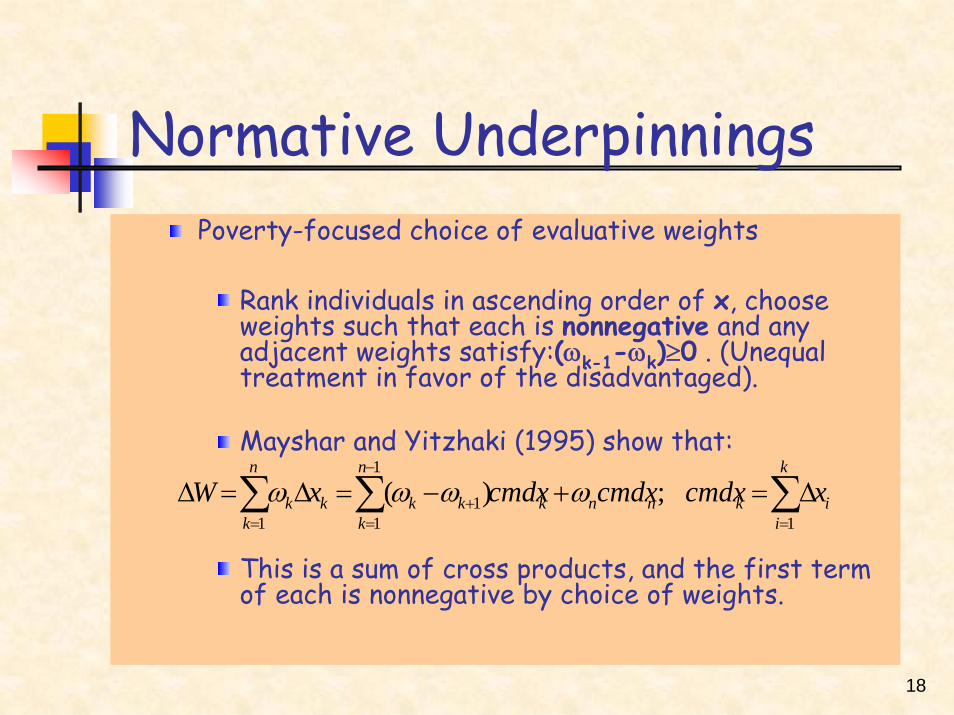
Normative UnderpinningsNormalize above by population size to get equivalent statement in terms of generalized Lorenz curves.Use ordinary Lorenz if both distributions have same mean.Thus second order dominance respects the Pigou-Dalton principle of transfers.It can also be shown that, social evaluation criteria of the Pigou-Dalton class respect the verdict of second order dominance.

21
Normative UnderpinningsThe Pareto Criterion and the Growth Incidence Curve.
Require that social weights be only nonnegative. Then Pareto improvement implies Δxk≥0 for all k.Alternatively
p
pLpL
xx
kxk
kk ∀≥
′′
=⇔∀≥Δ 1)()(0
00
11
0
1
μμ

22
Normative UnderpinningsLet g(p) stand for the growth rate at the pth
quantile, then the log transform of above expression yields:
This is equivalent to the growth incidence curve (Ravallion and Chen 2003)This is a distribution-adjusted, where adjustment factor is based on changes in the slope of the Lorenz curve.
)(ln)( pLpg ′Δ+= γ

23
Normative UnderpinningsIf Pareto improvement, then g(p)≥0 for all p. Well-known first order dominance results indicate that this change is poverty-reducing for a wide choice of poverty measures.

24
Normative Underpinnings
Growth Incidence Curves for Indonesia: 1993-2002
-2
0
2
4
6
8
10
12
14
0 10 20 30 40 50 60 70 80 90 100
Cumulative Percentage of Population
25
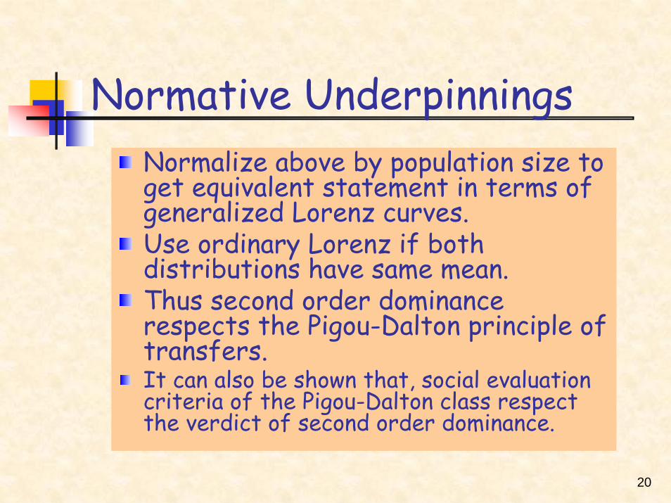
ParameterizationApproaches
Derive expression of Lorenz curve from known distribution function e.g. Lognormal or Beta. Then estimate structural parameters from data.Choose a functional form for the Lorenz curve.
Estimate its structural parameters from the data.Compute the curve and associated derivatives from parameter estimates.

26
ParameterizationThe General Quadratic Model (Datt 1992, 1998)
Regress [L(1-L) on (p2-L), L(p-1) and (p-L) with no intercept and dropping last observation.
Let β1, β2, β3 be the regression coefficients.

27
ParameterizationCompute the following:
21
22321
22121 )4();42();4();1( menrenme −=−=−=+++−= βββββββ
⎥⎦
⎤⎢⎣
⎡++++−= 2
122
2 )(21)( enpmpeppL β
)(42
2)(
22
2
enpmpnmppL++
+−−=′ β
8)()(
23
222 −++
=′′ enpmprpL

28
Parameterization
Rural India 1983: Regression Output for the General Quadratic Lorenz Representation of Household Expenditure
Coefficient Std. Error t-Statistic Prob.
BETA(1) 0.887734 0.006683 132.8389 0.0000 BETA(2) -1.451431 0.019062 -76.14295 0.0000 BETA(3) 0.202658 0.012847 15.77521 0.0000
R-squared 0.999959 Mean dependent var 0.121975 Adjusted R-squared 0.999950 S.D. dependent var 0.087678 S.E. of regression 0.000617 Akaike info criterion -11.73067 Sum squared resid 3.43E-06 Schwarz criterion -11.60944
Log likelihood 73.38399 Durbin-Watson stat 0.697503 Data Source: Datt (1998)

29
ParameterizationA Simulated Lorenz Curve for Rural India, 1983
0.0
0.2
0.4
0.6
0.8
1.0
0.0 0.1 0.2 0.3 0.4 0.5 0.6 0.7 0.8 0.9 1.0

30
Recovering the Size Distribution and Associated Measures of Inequality and Poverty
StrategyThe Extended Gini FamilyThe FGT Family of Poverty Measures

31
StrategyMost, if not all, inequality and poverty measures of interest can be computed from the following basic inputs:
the level of income or expenditure x, the associated density function f(x), and a poverty line (for poverty measures).
When relevant data are available, we can recover the first two inputs from a parameterized Lorenz function and the mean of the distribution.

32
StrategyIn particular, we derive x from the mean and the first order derivative of the Lorenz function. An estimate of the density function is obtained from the mean and the second order derivative.For computational purposes, we use the fact that f(x)dx is interpreted as the proportion of the population with income or expenditure in the close interval [x, dx] for a level of x and an infinitesimal change dx (Lambert 2001)

33
StrategyAbove considerations suggest applying numerical integration to the standard definitions of the measures of interest.
This obviates the need to derive special expressions for these indicators from the chosen functional form of the Lorenz curve (an approach followed by Datt 1992, 1998 for instance).
Focus on Gini and FGT

34
The Extended Gini FamilyThe ordinary Gini coefficient is equal to the area between the Lorenz curve and the line of complete equality (also known as the 45-degree line) divided by the whole area under the 45-degree line.Ordinary Gini is a member of an extended family based on a focal parameter that is interpreted as an indicator of inequality aversion.

35
The Extended Gini FamilyA covariance-based expression of the extended Gini coefficient can be derived from an abbreviation of the transfer-approving social evaluation criterion studied above.
where)()( ωnVxW =
),cov()( ωμμω ω xV x +=

36
The Extended Gini FamilyWith no loss of Generality, normalize average social weight to 1 (i.e. μω=1 )
Analogy with equally distributed equivalent income or expenditure ( see Atkinson 1970)A general expression of the extended Gini coefficient is therefore:
)](1[]),cov(1[),cov()( ωμμ
ωμωμω GxxV xx
xx −=+=+=
x
xGμ
ωω ),cov()( −=

37
The Extended Gini Family
For computational purposes, we adopt the system of weights proposed by Yitzhaki (1983)
Where pk is the proportion of people with income less than or equal xk, and ν is the focal parameter indicating the degree of inequality aversion.
1)1()( −−= νννω kk p

38
The Extended Gini Family(Evaluative Weights as a Function of the Focal Parameter ν)
0
1
2
3
4
5
6
7
0.0 0.1 0.2 0.3 0.4 0.5 0.6 0.7 0.8 0.9 1.0

39
The Extended Gini Family
Cut-off Rank as a Function of the Aversion Parameter.
υ 1.1 1.2 1.5 2.0 3 6 10 20 30 50 100 200 p* 0.62 0.60 0.56 0.50 0.42 0.30 0.23 0.15 0.11 0.08 0.05 0.03
Source: Essama-Nssah (2002)

40
The Extended Gini FamilyThe corresponding expression for the extended Gini is:
It can also be computed as:
])1(,cov[)( 1−−−= ν
μνν pxG
x
])1(),(cov[)( 1−−′−= νμμνν ppLG x
x

41
The Extended Gini Family
Alternatively, the extended Gini coefficient can be written as:
Chotikapanich and Griffiths (2001) propose a linear segment estimator defined as follows:
∫ −−−−=1
0
2 )()1()1(1)( dppLpG νννν
∑∑
=
−=
=−−−⎟⎟⎠
⎞⎜⎜⎝
⎛+= m
jjj
kkkkk
m
k k
k
xw
xwpp
wG
1
11
];)1()1[(1)( θθ
ν νν

42
The Extended Gini Family
The linear segment estimator is equivalent to:
When the focal parameter ν is equal to 2, we get the ordinary Gini index.
[ ]∑=
−−−−Δ
Δ+=
m
kkk
k
k ppppL
G1
1 )1()1()(
1)( ννν

43
The Extended Gini Family
Sen’s measure of poverty is a close relative of the Gini coefficient.
Let μp and Gp(ν) be respectively the average income and the extended Gini for the poor. The extended Sen index of poverty is equal to:
⎥⎦
⎤⎢⎣
⎡ −−=
zG
HS pp )](1[1)(
νμν
44
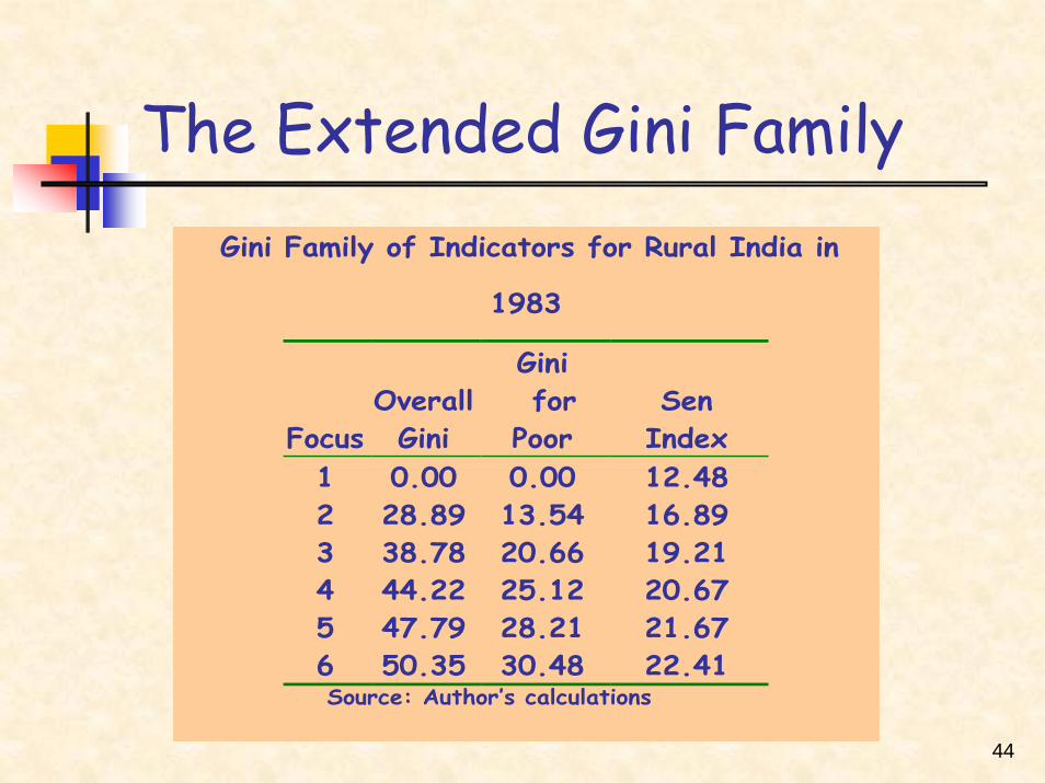
The Extended Gini Family Gini Family of Indicators for Rural India in
1983
Focus Overall Gini
Gini for
Poor Sen
Index 1 0.00 0.00 12.48 2 28.89 13.54 16.89 3 38.78 20.66 19.21 4 44.22 25.12 20.67 5 47.79 28.21 21.67 6 50.35 30.48 22.41 Source: Author’s calculations

45
The FGT Family of Poverty Measures
Kakwani(1999) defines a class of additively separable poverty measures starting from the notion of deprivation. Let ψ(z,xi) stand for an indicator of deprivation at the individual level. A class of additively separable poverty measures can be defined as:
ii
n
i
n
i i
ii xxf
ppL
zxzn
xzP Δ⎟⎟⎠
⎞⎜⎜⎝
⎛Δ
Δ== ∑ ∑
= =
)()(
,),(1),(1 1
μψψ

46
The FGT Family of Poverty Measures
Deprivation felt by an individual depends only on a fixed poverty line and her level of welfare and not on the welfare of other individuals in society.
When population is divided exhaustively into mutually exclusive socioeconomic groups, overall poverty is a weighted average of poverty in each group.
The weights are population shares. Hence these measures are also additively decomposable.

47
The FGT Family of Poverty Measures
Specification of the deprivation function leads to particular members of the class.For Foster-Greer-Thorbecke(1984), expression due to Jenkins and Lambert (1997):
}.0,)/1max{(),( αψ zxxz iiFGT −=

48
The FGT Family of Poverty Measures
α is an indicator of aversion for inequality among the poor.
When α=0, we get the headcount index; When α=1, we get the poverty gap index; and When α=2, we get the squared poverty gap index.

49
The FGT Family of Poverty Measures
TIP Representation of Poverty (Jenkins and Lambert 1997)
TIP stands for the Three “I”s of Poverty: incidence, intensity, and inequality (among the poor).
The curve provides a graphical summary of those three dimensions of poverty.Construction analogous to that of Lorenz curve.

50
The FGT Family of Poverty Measures
Step 1: rank individuals from poorest to richest.Step 2: compute relative poverty gaps, gi=max{(1-xi/z), 0}.Step 3: form cumulative sum of poverty gaps normalized by population size.Step 4: plot result as function of cumulative population shares:
0)0(;;1)(1
=== ∑=
JLnkpg
npJL
k
ii

51
The FGT Family of Poverty Measures
A TIP Curve for Rural India in 1983
.00
.02
.04
.06
.08
.10
.12
.14
0.0 0.1 0.2 0.3 0.4 0.5 0.6 0.7 0.8 0.9 1.0
52
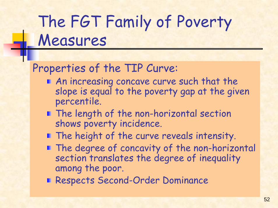
The FGT Family of Poverty Measures
Properties of the TIP Curve:An increasing concave curve such that the slope is equal to the poverty gap at the given percentile.The length of the non-horizontal section shows poverty incidence.The height of the curve reveals intensity.The degree of concavity of the non-horizontal section translates the degree of inequality among the poor.Respects Second-Order Dominance

53
Decomposition of Poverty Outcomes
Poverty measures are computed on the basis of a distribution of an indicator of the living standard. Such a distribution is fully characterized by the mean and the degree of relative inequality.It is therefore reasonable to think of poverty outcomes as determined by these two factors.We focus on the elasticity approach and the Shapley method of decomposing poverty outcomes.
54
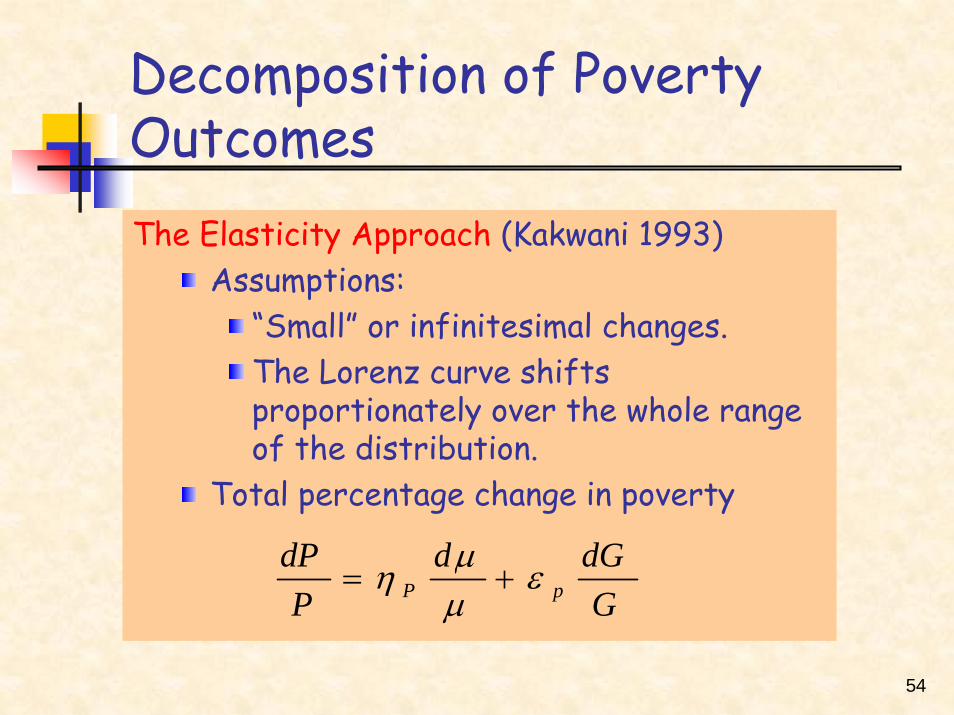
Decomposition of Poverty OutcomesThe Elasticity Approach (Kakwani 1993)
Assumptions:“Small” or infinitesimal changes.The Lorenz curve shifts proportionately over the whole range of the distribution.
Total percentage change in poverty
GdGd
PdP
pP εμμη +=

55
Decomposition of Poverty Outcomes
Where ηp stands for the growth elasticity of the poverty index, μ is the mean of the distribution, εp represents the elasticity of the poverty index with respect to the ordinary Gini coefficient, G.
Setting the proportional change in poverty equal to zero leads to a indicator of the trade-off between mean income growth and inequality.

56
Decomposition of Poverty Outcomes
The indicator is known as the marginal proportional rate of substitution between mean income and inequality (Kakwani 1993).
This is a measure of the extent to which income needs to grow to compensate for an increase of 1 percent in the Gini index.
P
PGG
MPRSηε
μμ
−=∂∂
=

57
Decomposition of Poverty Outcomes
For the class of additively separable poverty measures, the general formula for the growth elasticity is:
The elasticity with respect to Gini is:
wh stands for the relative frequency of observation xh.
∑=
⎟⎟⎠
⎞⎜⎜⎝
⎛∂∂
=m
h hhhP x
xwP 1
1 ψη
∑=
⎟⎟⎠
⎞⎜⎜⎝
⎛∂∂
−=m
h hhPP x
wP 1
ψμηε

58
Decomposition of Poverty Outcomes
For the headcount index:the growth elasticity is:
The elasticity with respect to Gini is:
0)(<−=
Hzzf
Hη
HH zz ημε )( −
−=

59
Decomposition of Poverty Outcomes
For the rest of the FGT family, these parameters have the following expressions:
.0
;
;][
1
1
>
+=
−−=
−
−
α
αμηε
αη
α
α
α
αα
zPP
PPP
FGTFGT
FGT

60
Decomposition of Poverty Outcomes
FGT and Associated Elasticity Measures for Rural India,1983
Focus FGT Growth Inequality 0 45.07 -1.87 0.44 1 12.48 -2.61 1.85 2 4.75 -3.25 3.23
Source: Author’s calculations

61
Decomposition of Poverty Outcomes
Ravallion (1994b) argues that the elasticity approach may lead to large errors in the case of big discrete changes. In these cases, it is preferable to use the mean and the Lorenz curve to decompose changes in poverty into growth and inequality components.Ravallion and Datt (1992) propose a
method that leaves a residual (interpreted as an interaction term).

62
Decomposition of Poverty Outcomes
Kakwani (1997) and Shorrocks (1999) offer another approach to the decomposition that does not involve a residual. We focus on this one. Shorrocks (1999) rationalizes the approach with reference to the Shapley value of a cooperative game. In such a game, partners join forces to produce a good that must be shared. This raises the issue of fair division.

63
Example of Division of Common Property
Birhor Rule for Sharing the Kill after a Monkey Hunt Claimants Share Spirits of the Chase A bit of meat roasted by
Chief Tribal Chief Neck and half of back meat
of each animal in addition to his hunter’s share
Beater Equal share of entrails, tails and feet based on number of beaters
Owner of Net Hind leg Flanker Hind leg Chief’s Hunter [not specified in source
document] Source: Young(1994). Note: “Any left over is divided into as many portions as there are eligible persons, plus an extra share for the chief”. The Birhors are a tribe in east-central India.

64
Decomposition of Poverty Outcomes
Example: Cost Sharing (Young, 1994)“Given a cost-sharing game on a fixed set of players, let the players join the cooperative enterprise one at the time in some predetermined order. As each player joins, the number of players to be served increases. The player’s cost contribution is his net addition to the cost when he joins, that is the incremental cost of adding him to the group of players who have already joined. The Shapley value of a player is his average cost contribution over all possible orderings of players”

65
Decomposition of Poverty Outcomes
Interpretation of the above principle in the context of poverty decomposition leads to the following expressions.
The Shapley contribution of growth to change in poverty:
[ ] [ ]),(),(21),(),(
21
11122122 LPLPLPLPSG μμμμ −+−=

66
Decomposition of Poverty Outcomes
The Shapley contribution of inequality is:
The following value judgments underpin the Shapley method:
Symmetry or anonymity (the identity or label of a factor is irrelevant)Rule should lead to exact decompositionContribution of each factor is equal to its first round marginal impact.
[ ] [ ]),(),(21,(),(
21
11211222 LPLPLPLPSL μμμμ −+−=

67
Decomposition of Poverty Outcomes
A Profile of Poverty in Indonesia, 1993-2002
Poverty Measures 1993 1996 2002
Headcount 61.55 50.51 52.42
Poverty Gap 21.03 15.33 15.68
Squared Poverty Gap 9.16 6.02 6.09
Source: Author’s simulations (poverty line about $2/day)

68
Decomposition of Poverty Outcomes
Shapley Decomposition of Poverty Outcomes in Indonesia,
1993-2002
Measure Total Change Growth Inequality Headcount -9.13 -12.49 3.36 Poverty Gap -5.35 -6.87 1.52 Squared Poverty Gap
-3.07 -3.82 0.75
Source: Author’s simulations

69
Decomposition of Poverty Outcomes
Shapley Decomposition of Poverty Outcomes in Indonesia,
1996-2002
Measure Total Change Growth InequalityHeadcount 1.91 4.05 -2.14 Poverty Gap 0.35 2.04 -1.69 Squared Poverty Gap 0.07 1.07 -1.00 Source: Author’s Simulations

70
Summary
The use of numerical integration in simulating inequality and poverty measures obviates the need to derive special expressions from the chosen functional form of the Lorenz curve.
Lorenz ranking of distributions respects the Pigou-Dalton principle of transfers underlying Second-Order Dominance.
Ranking by the GIC is consistent with the Pareto criterion underlying First-Order Dominance
When dominance tests fail, one can resort to aggregate indicators for inequality and poverty comparisons.

71
Summary
All measures reviewed here depend to some extent on a focal parameter that can be interpreted as an indicator of aversion for inequality.
The aversion parameter allows the analyst to calibrate the poverty focus of social impact assessment.
The use of the Lorenz curve facilitates the decomposition of poverty outcomes in terms of changes in the mean and in relative inequality.

72
References
Atkinson, A. B. 1970. On the Measurement of Inequality. Journal of Economic Theory, 2, 244-263.Chotikapanich, Duangkamon and Griffiths, Willianm. 2001. On the Calculation of the of the Extended Gini Coefficient. Review of Income and Wealth. Series 47, No. 4: 541-547.Datt, Gaurav. 1998. Computational Tools for Poverty Measurement and Analysis. Washington D.C.: International Food Policy Research Institute (IFPRI) Discussion Paper No.50 (Food Consumption and Nutrition Division).

73
References
_________. 1992. Computational Tools for Poverty Measurement and Analysis. Washington D.C.: The World Bank.Essama-Nssah, B. 2002. Assessing the Distributional Impact of Public Policy. Policy Research Working Paper No. 2883. Washington, D.C.: The World Bank.Foster J., Greer, J. and Thorbecke, E. 1984. A Class of Decomposable Poverty Measures. Econometrica, Vol. 52, No.3 , 761-766. (May).

74
ReferencesJenkins, S. and Lambert, Peter J. . 1997. Three ‘I’s of Poverty Curves, with Analysis of UK Poverty Trends. Oxford Economic Papers, 49: 317-327.Kakwani, Nanak. 1999. Inequality, Welfare and Poverty: Three Interrelated Phenomena. In Jacques Silber (ed.) “Handbook of Income Inequality Measurement”. Boston: Kluwer Academic Publishers.Lambert, Peter J. 2001. The Distribution and Redistribution of Income. Manchester: Manchester University Press.

75
ReferencesMayshar, Joram and Yitzhaki, Shlomo. 1995. Dalton-Improving Indirect Tax Reform. The American Economic Review, Vol. 85, No. 4: 793-807.Ravallion, Martin. 1994. Poverty Comparisons. Chur: Harwood Academic.Ravallion, Martin, and Chen, Shaohua. 2003. Measuring Pro-Poor Growth. Fconomics Letters 78, 93-99.Ravallion Martin and Datt Gaurav. 1992. Growth and Redistribution Components of Changes in Poverty Measures: A Decomposition with Application to Brazil and India in the 1980s. Journal of Development Economics 38:275-295.

76
ReferencesSen, Amartya. 1992. Inequality Reexamined. New York: Russell Sage FoundationYitzhaki, Shlomo. 1983. On an Extension of the Gini Index of Inequality. International Economic Review, Vol. 24, No 3: 617-628.
77
The End.