The Long-term Impact of Public Health Measures

Targeting Children∗

Lauren Hoehn-Velasco†

May 12, 2018[Updated Version]

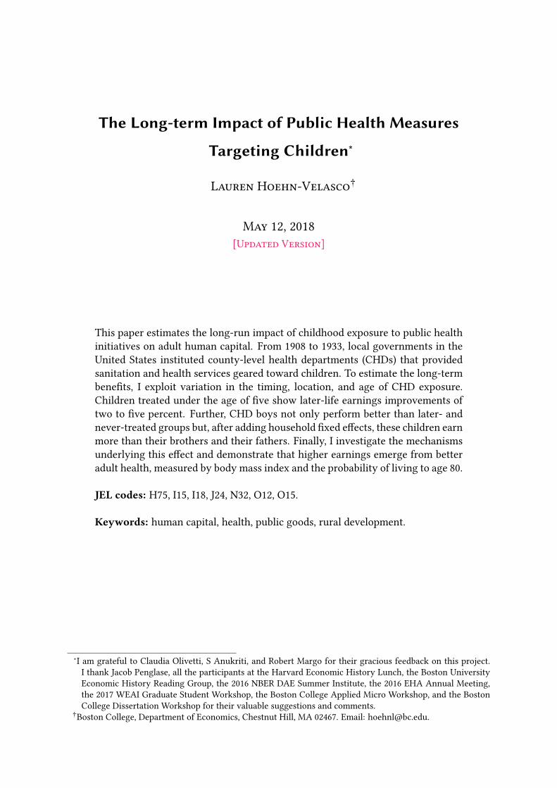
This paper estimates the long-run impact of childhood exposure to public healthinitiatives on adult human capital. From 1908 to 1933, local governments in theUnited States instituted county-level health departments (CHDs) that providedsanitation and health services geared toward children. To estimate the long-termbene�ts, I exploit variation in the timing, location, and age of CHD exposure.Children treated under the age of �ve show later-life earnings improvements oftwo to �ve percent. Further, CHD boys not only perform better than later- andnever-treated groups but, after adding household �xed e�ects, these children earnmore than their brothers and their fathers. Finally, I investigate the mechanismsunderlying this e�ect and demonstrate that higher earnings emerge from betteradult health, measured by body mass index and the probability of living to age 80.

JEL codes: H75, I15, I18, J24, N32, O12, O15.

Keywords: human capital, health, public goods, rural development.

∗I am grateful to Claudia Olivetti, S Anukriti, and Robert Margo for their gracious feedback on this project.I thank Jacob Penglase, all the participants at the Harvard Economic History Lunch, the Boston UniversityEconomic History Reading Group, the 2016 NBER DAE Summer Institute, the 2016 EHA Annual Meeting,the 2017 WEAI Graduate Student Workshop, the Boston College Applied Micro Workshop, and the BostonCollege Dissertation Workshop for their valuable suggestions and comments.

†Boston College, Department of Economics, Chestnut Hill, MA 02467. Email: hoehnl@bc.edu.

1 Introduction

Today in the United States nearly one out of every ten dollars in the economy is spentas public expenditures on health.1 By contrast, in 1900, public expenditure on health made uponly one out of every 200 dollars.2 At that time, the U.S. government put more resources intothe health of farm animals, plants, and birds than into the health of its citizens.3 Determiningwhether the twenty-fold increase in public spending produced corresponding welfare gainsis a di�cult question to answer in aggregate. Both health and welfare have increased over thepast 100 years, but this correlation does not express the causal connection between the two.While studies have established short-run bene�ts to public spending on health,4 less is knownabout the long-run welfare bene�ts. Understanding whether public expenditure produceslong-run welfare gains is imperative for properly valuing public investment in health.

This study asks whether public expenditure on health produces lasting welfare gainsthroughout the lifespan of individuals. To causally address this question, I follow childrenexposed to a particular public health program into adulthood to measure their income gains.I focus on a public health infrastructure rollout over 1908 to 1933. This movement establishedcounty health departments (CHDs) in rural areas of 38 states and brought sanitation and ba-sic health services to rural children for the �rst time in U.S. history. The broad scope andthe historical lens of the study allows me to see the full lifespans of boys exposed to the pro-gram using a century-long longitudinal dataset. I construct this dataset by linking togetherfour separate datasets: CHD administrative records, 1920 and 1940 census data, World WarII enlistment records, and social security death records. This allows me to identify childhoodexposure to the health program and then follow up with early adult earnings, adult health,and the death year.

To determine the e�ect of improved childhood health on later-life earnings, I exploit vari-ation in CHD location, the staggered timing of the intervention, and the age of treatment.5

Children residing in a CHD county while under the age of �ve form the treatment group.This assignment creates three control groups for the health e�ects. First, within the samecounty, children treated under age �ve are compared against older cohorts. This comparisonenables the inclusion of county �xed e�ects, which remove time-invariant county characteris-tics. Second, across treated and never-treated counties, children are compared over each yearof birth. Third, the staggered adoption of CHDs over 1908 to 1933 compares children across

18.3% of GDP is spent as public expenditure on health (World Bank [2014])2In 1900 0.55% of US GDP (Fishback [2010])3“The federal government, which spent millions of dollars on diseases of farm animals, birds, and plants in the

nineteenth century, spent almost nothing on the health of its citizens" (Du�y 1993)4For short-run e�ects in historical context see: (?, ?, Haines (2001), Cutler and Miller (2005), and Alsan and

Goldin (2015).5Using variation in the age of exposure builds upon related work of Du�o (2001).

2

birth year for early and later-treated counties.6 This comparison of early and later-treatedchildren mitigates remaining concern over both selection into treatment as well as changes incohort-speci�c wage patterns. Finally, to capture the presence of children in CHD counties,the treatment assignment is based on the child’s location during the 1920 and 1930 census.This childhood exposure is then linked to later-life outcomes using the 1940 census.

I �nd that children exposed to a CHD before the age of �ve earned two to �ve percentmore in adulthood than the comparison groups. Testing additional measures of income, in-cluding the hourly wage, occupational score, and intergenerational occupational mobility, re-veals comparable earnings improvements. Further, I add household �xed e�ects to the model,instead of county �xed e�ects, which renders a stronger interpretation of the baseline results.CHD children not outperform control groups, but they perform better in their labor marketthan their older brothers and their fathers. The similarity between the estimates using house-hold �xed e�ects and county �xed e�ects supports a causal interpretation of the impact of theCHD.7

Next, I relax the assumption on the treatment cohort by employing an indicator for ex-posure during each year of childhood, from pre-birth to age 10. Here, I �nd that the earningsimprovement is highest for children who received health services in infancy and decreasesin magnitude over each year of childhood. For children exposed in utero and infancy, theincrease in income is between six and eight percent. Grounding the relative size of the ef-fect in returns to schooling reveals that health improvements in infancy are comparable toan additional year of schooling. For treatment before age �ve, CHD exposure is equivalent toone-half of a year of schooling.8

To understand how CHDs produced income gains, it is necessary to appreciate the stateof rural health in the early twentieth century. While bucolic sentiment suggests that ru-ral schoolchildren were disease-free, when compared with their urban counterparts, studiesduring the beginning of the twentieth century reveal a di�erent story. Davenport and Love(1920) examine defects in men drafted into the US military and �nd that, though cities sur-passed rural areas in the rate of defects, the overall health condition was "counterbalanced bythe greater amount in rural districts of mental de�ciency, deformed and defective extremities,blindness in one eye, arthritis and ankylosis and gonococcus infection." Davenport and Love(1920) further note that the majority of deformities found in rural areas originate in infancy,which lends credibility to �ndings that suggest higher prenatal e�ects of CHDs. A similarlarge-scale study of one-half of a million schoolchildren reports that "children attending rural

6For the income results, an arbitrary cuto� for young exposure occurs in 1925 based on the availability of the1920 census. This 1920 census is the main data source used to identify the location of children during therollout.

7The baseline results are also robust to the inclusion of 1940 county �xed e�ects, as well as county time trends.8Clay et al. (2016) �nd the period return to schooling to be 0.064 to 0.079.

3

schools are, on the average, less healthy and are handicapped by more physical defects thanthe children of the cities, including all the children of the slums" (?). In both studies, the im-plication is similar; rural children were poised to bene�t from access to the health servicesprovided by the CHDs. This program was the �rst major expansion of health infrastructureto rural areas and one of the largest wholesale expansions in US history.

To investigate the underlying mechanisms behind the income improvements, I evaluatethe respective roles of adult schooling and health. In related literature,9 morbidity declineslead to higher educational attainment for schoolchildren. Results here paint a di�erent picture;exposed children show no di�erence in their total years of schooling. Instead, treated childrenare more likely to maintain the correct grade level for their age. This reduced grade regressionshows that children are more productive while in school, despite not increasing their totalinvestment in education. The rise in school performance hints at earnings increases emergingdirectly from higher health human capital.10

To consider the direct e�ect on adult health, I take advantage of the cognitive scores, bodymass index (BMI), and height reported in World War II army enlistment records (WWII) aswell as lifespan, published in the Social Security Death Master File (SSDM). Reduced diseaseexposure in childhood may have one of two e�ects on adult health. First, the reduction inillness severity and frequency may reduce disability in surviving adults. Second, throughreduced mortality selection, less healthy and resilient adults may survive. To test which e�ectdominates, I link health measures from the SSDM and WWII data to the 1930 census. Basedon this sample, I �nd evidence of both decreased mortality selection and lower disability.Men exposed to a CHD in childhood have higher BMI and an increased likelihood of livingpast age 80. These men, however, also have a lower probability of reaching age 60 and areslightly shorter. These contrasting e�ects suggest that, while the healthiest individuals aregetting healthier, mortality selection may allow the least healthy individuals to survive pastchildhood.

This study complements a broad literature linking childhood health improvements to life-long economic outcomes (Behrman and Rosenzweig (2004), Almond (2006), Bleakley (2007),Case et al. (2008), Case and Paxson (2009), Currie (2009), Bozzoli et al. (2009), ?, Currie and Al-mond (2011), and Beach et al. (2016)). These studies have demonstrated that childhood healthhas a lifelong in�uence on adult productivity and well-being. The present study also addsto the extensive literature measuring the e�ectiveness of public health interventions (?, ?,Haines (2001), Cutler and Miller (2005), and Alsan and Goldin (2015)). A primary focus of this

9See the empirical strategy in Bleakley (2007).10Grade regression may su�er from measurement issues due to ungraded Southern schools. Such schools did

not assign students to class levels, and this issue persisted into the 1940 census for the South. Enumeratorsin 1940 were instructed to make their best guess grade level, based on the child’s reported age. For furtherexplanation on the issue, see ?, ?, and Collins and Margo (2006).

4

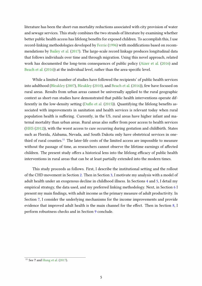
literature has been the short-run mortality reductions associated with city provision of waterand sewage services. This study combines the two strands of literature by examining whetherbetter public health access has lifelong bene�ts for exposed children. To accomplish this, I userecord-linking methodologies developed by Ferrie (1996) with modi�cations based on recom-mendations by Bailey et al. (2017). The large-scale record linkage produces longitudinal datathat follows individuals over time and through migration. Using this novel approach, relatedwork has documented the long-term consequences of public policy (Aizer et al. (2016) andBeach et al. (2016)) at the individual level, rather than the area-speci�c level.

While a limited number of studies have followed the recipients’ of public health servicesinto adulthood (Bleakley (2007), Bleakley (2010), and Beach et al. (2016)), few have focused onrural areas. Results from urban areas cannot be universally applied to the rural geographiccontext as short-run studies have demonstrated that public health interventions operate dif-ferently in the low-density setting (Du�o et al. (2015)). Quantifying the lifelong bene�ts as-sociated with improvements in sanitation and health services is relevant today when ruralpopulation health is su�ering. Currently, in the US, rural areas have higher infant and ma-ternal mortality than urban areas. Rural areas also su�er from poor access to health services(HHS (2012)), with the worst access to care occurring during gestation and childbirth. Statessuch as Florida, Alabama, Nevada, and South Dakota only have obstetrical services in one-third of rural counties.11 The later-life costs of the limited access are impossible to measurewithout the passage of time, as researchers cannot observe the lifetime earnings of a�ectedchildren. The present study o�ers a historical lens into the lifelong e�cacy of public healthinterventions in rural areas that can be at least partially extended into the modern times.

This study proceeds as follows. First, I describe the institutional setting and the rolloutof the CHD movement in Section 2. Then in Section 3, I motivate my analysis with a model ofadult health under an exogenous decline in childhood illness. In Sections 4 and 5, I detail myempirical strategy, the data used, and my preferred linking methodology. Next, in Section 6 Ipresent my main �ndings, with adult income as the primary measure of adult productivity. InSection 7, I consider the underlying mechanisms for the income improvements and provideevidence that improved adult health is the main channel for the e�ect. Then in Section 8, Iperform robustness checks and in Section 9 conclude.

11 See ? and Hung et al. (2017).

5

2 Background

At the turn of the twentieth century, 60 percent of the US population lived in rural areaswithout access to public health services.12 The interstate spread of disease,13 as well as theclear gap in health services between urban and rural areas,14 motivated the United StatesPublic Health Service (USPHS) to develop a strategy to provide public health to the entirenation.15 This desire combined with initial surveys in "18 fairly representative counties in 16states" (Ferrell et al. (1936) p. 4) established the CHD movement in the US. While the CHDmovement was the byproduct of a national e�ort, CHDs were locally administered units thatserved the countryside as well as towns with less than 10,000 individuals.

The rollout of the CHDs began in 1908 and occurred over three waves. In the initial years1908-1914, local governments were responsible for funding but received consultation servicesfrom organizations such as the USPHS and the Rockefeller Sanitary Commission (RSC). Thenin 1915, state governments, the USPHS, and the RSC began to o�er grants to increase programadoption. During the 1920s, additional support was provided from public and private fundingsources. One notable development was the Sheppard-Towner Act of 1921, which delivered aidfor initiatives targeting mother and infant health. The in�ow of funding for children helpedCHDs to increase provision of prenatal and newborn exams, improve the training of midwives,and spread mother-infant hygiene information.

By 1933 CHDs were distributed throughout 38 states. Figure I displays a map of thecounties a�ected by the movement. Panel A presents the spread of CHDs throughout the US,with dark blue areas representing the adoption of a CHD between 1908 and 1933. Panel Bshows the percentage of funds from external sources, which include the RSC, USPHS, statefunds, and other private donors. External funds vary between counties and states, with somereceiving no external aid, and others receiving all of their funding from external sources. Anotable attribute of the map is the absence of services in New England and several Midwesternstates. The structure of local government accounts for the state-level di�erences in adoptionof the movement. In New England and the central Midwest, the township, instead of thecounty, acts as the main political unit and provides most of the public goods, including sanitary

12 City health departments had evolved so that, by 1873, 134 cities in the United States had boards of health, andthough many did not initially have full-time health o�cers, by 1900 the majority did (Altenderfer (1946)).

13Disease was a�ecting commerce and "frequent instances were observed in which cases of diseases developingin the city had been caused by infection brought in through the medium of persons and of water, milk,oysters, or some other food supply from a nearly or distant rural community" (Ferrell et al. (1936) p. 2).

14Comparable programs in cities existed prior to the CHD movement. Ferrell et al. (1936) notes that, at thetiming of the �rst CHD, "cities and towns had developed health services, but for the rural areas very littlehad been done" (p. III).

15"The Public Health Service as the Federal agency especially concerned and speci�cally authorized to cooperatewith State and local health departments to prevent the spread of human infections between the States" (Ferrellet al. (1936) p. 1).

6

administration (Chapin (1900)).16 In the South and West, on the other hand, "the county boardof health has ... been established to look after the sanitary interests of the people outside ofthe incorporated municipalities" (Chapin (1900)). Due to the structural di�erences in localgovernance, the township-organized states opted out of the county-level service.17 To accountfor the state-level di�erence in structure, only the 38 treatment states are included in theanalysis. A more extensive discussion of di�erences in state-level adoption is included inAppendix Section ??.

For states that did adopt the movement, the presence of a CHD is de�ned as having afull-time health o�cer dedicated to the operation of public health services at the county level.Before the movement, while a few counties did have part-time boards of health, these healthboards were sta�ed by physicians whose time was dedicated to private practice. The existingboards were weak, ine�ective, and improperly funded (Chapin (1900)). By contrast, formalCHDs were full-time units that operated under the direction of a full-time health o�cer alongwith assistance from nurses, inspectors, and clerks. These CHDs provided annual salaries forthe employees and ensured the health o�cers and nurses were focused on providing publichealth services, instead of working in private practice Figure II provides a diagram of thestructure of CHDs as well as the speci�c activities completed by each sta� member.

To better understand the exact activities performed by CHDs, ? provides a cross sectionof services for a select 132 counties.18 An example entry of the original table is provided inTable ??, with the summary statistics in Panel A of Table 1. These aggregate statistics forsanitation and medical e�orts are reported per thousand persons and averaged over the years1925 through 1928. To combine activities, I only include those that would require the presenceof a trained sta� member. This requirement would incorporate the installation of a toilet orthe number of exams given, as both activities would require an health o�cial to be present.

CHD health services primarily focused their e�orts on examinations of children. Theseexaminations served infants, preschool-aged children, schoolchildren, and pregnant women,with services provided for free for those who could not pay. During the exam, doctors andnurses sought to identify health concerns, administer medication and vaccines, and providegeneral advice to parents including the importance of breastfeeding. Exams were conductedby the health o�cers and nurses in both clinics and at home. Based on the numbers pro-vided, CHDs examination e�orts were enough to cover 40-100 percent of the population. In

16The regional di�erences in the political divisions was not a new occurrence and evolved over time, beginningwith the local government in the colonial era (Chapin (1900) p. 6).

17These states include the New England states, Illinois, Iowa, Michigan, Minnesota, New Jersey, New York,Ohio, Pennsylvania, and Wisconsin. Ohio and Michigan later passed laws that required the organization ofcounty-level services to ensure rural areas received services. See the Hughes Act in Ohio.

18This document o�ers a snapshot into precise CHD activities for select health departments funded by theUSPHS and is an additional source of information from the main data source utilized in the analysis section(Ferrell et al. (1936)).

7

the table, CHD e�orts are shown per capita for the targeted population, and for infants thenumber of exams was enough to almost examine each infant twice. For an illustration of theexaminations see Figure III.

To complement the examinations, CHD public health nurses and medical o�cers pro-vided nutritional advice; communicable disease control; vaccinations for typhoid, smallpox,and diphtheria; as well as instruction to local midwives and schools. These medical e�orts areshown in the bottom panel of Table 1. Midwife training is excluded from the table, though it isstill an important medical e�ort to note. In 1930 alone, CHDs provided "instruction of 12,880midwives in cleanly and careful methods" (? p. 2632). In rural areas, as access to doctors waslimited, midwives were frequently the default care provider, especially in poorer locales.

2.1 Health E�ects of CHDs

Based on the historical literature’s anecdotal claims of CHDs successes, I evaluate theempirical evidence for the e�ectiveness of CHDs. There are three primary channels that Iconsider: mortality, morbidity, and fertility. The overall impacts of the CHD on each channelare as follows:

[1] Reduced mortality for infants (by two per 1,000 births)

[2] Decreased maternal mortality (two per 1,000 births)

[3] Declines in morbidity (between �ve and ten cases per 10,000)

[4] No e�ect on birth rate

I discuss the details of each empirical strategy in Appendix Section ??.

3 Conceptual Framework

The conceptual framework builds upon the work of ?, which takes the structure of Gross-man (1972) and modi�es the traditional representation of health as an investment good to asequential investment setting. I recast this framework to an environment where parental in-vestments in childhood directly impact adult health. Adult health is based on three factors:the disease environment in early childhood, the parental care in early childhood, and the sub-sequent educational choices. This section outlines the portion of the model necessary forintuition, with the full maximization relegated to Appendix Section ??.

8

3.1 Health Production Function

The production of adult health for each child is a function of the parental choice of child-hood education e and care c as well as the exogenous illness prevalence φ:

h = h(e, c, φ) (1)

where the health production function is increasing in e and c, and decreasing in φ.

Since CHD bene�ts are contained to early childhood, child health is established beforemaking educational investments. I reexpress this dynamic process as a (static) reduced-formrepresentation by re-writing adult health as a function of both the childhood health and thedisease level (?). Within adult health, childhood health, x, is formed based on the parentalcare and the exogenous disease levels, rewritten as x(c, φ). Then, the educational investmentrelies on the �nal childhood health, expressed as e(x).19 Based on these adjustments, the adulthealth appears as a consumption of complements:

h = h(e(x), x(c, φ)) (2)

The primary focus of the production function is to clarify how exogenous shocks to illnesslevels, φ, will impact childhood health, x, and thereby adult health, h.

Consider an exogenous reduction in disease levels, φ. In this setting, there are two typesof children, those who would have survived without the reduction in illness and those whowould not have survived without the shock.20 First, children who would have survived beforethe decline in illness unambiguously experience lower scarring in childhood. These childrenwill have greater childhood health human capital, x, and higher adult health, h. Second,children who would have died before the decline in illness are now able to survive. Thesechildren survive, despite lower levels of care, c, and childhood health, x. Due to the reducedmortality selection, the lower childhood health, x, may result in lower levels of adult health,h. As the adult health of these children would have been absent from the population beforethe decline in illness, their survival may reduce average adult health.

To formally examine the relationship between the disease environment and adult health,the e�ect of the disease environment can be expressed as the total derivative of hwith respectto φ:

19Childhood health is increasing in parental care c and decreasing in illness episodes φ.20This captures both scarring and selection or survival bias discussed in the literature, as in Bozzoli et al. (2009).

9

dh

dφ=dh

dx

dx

dφ=

(∂h

∂e

∂e

∂x+∂h

∂x

)(∂x

∂φ+∂x

∂c

∂c

∂φ

)(3)

where the relationship between adult health and illness levels, dhdφ

, is composed of the rela-tionship between adult health and child health, dh

dx, and the relationship between childhood

health and the illness levels, dxdφ

.

The relationship between child health and the disease environment, dxdφ

, decomposes to∂x∂φ

+ ∂x∂c∂c∂φ

. The �rst portion, ∂x∂φ

, represents the scarring e�ect of the disease environmenton childhood health (the biological component). The second portion, ∂x

∂c∂c∂φ

, describes theparental role in maintaining child health. If scarring is large, or parental care is ine�ective,then reducing φ will be unambiguously bene�cial. In cases where care remediates the nega-tive health e�ects of illness, reducing φmay only bene�t children with low parental care andmortality selection may reduce overall health.

Now considering the relationship between adult and child health, dhdx

, the persistence ofhealth from early to later life appears as ∂h

∂e∂e∂x

+ ∂h∂x

. The �rst portion, ∂h∂e∂e∂x

, describes thedegree to which education can compensate for the negative e�ects of scarring in childhood.The second portion describes the relationship between childhood and adult health, ∂h

∂x. Here

again, if education can compensate for negative health e�ects, then the role of reducing illnessmay be small. If, on the other hand, childhood health directly in�uences adult health through∂h∂x

, then individuals will bene�t from the health investment through reduced scarring.

3.2 Model Implications

Within the conceptual framework, the e�ect of a reduction in illness levels, φ, on later-life income is ambiguous. The result depends on the relative response of each factor in Equa-tion 3 as well as the health e�ects in Section 2.1. First, poor childhood health may hinder theacquisition of human capital through e(x) and would reduce either quantity or the quality ofeducation. Second, scarring in childhood may directly impact adult health through childhoodhealth x. Third, the relationship between parental care, childhood health, and education is de-pendent on preferences and prices. Parents may focus their investment on childhood healthand fail to readjust education if the price of education is high or if the mitigating e�ect ofeducation is small, ∂h

∂e∂e∂x

.

Assume the disease exposure, φ, declines. The basic implications are as follows:

Implication 1 Reversal of Mortality Selection: Relatively large mortality reductionsmay allow children with lower levels of parental care (c) to survive. This reduction in

10

mortality selection may decrease the population’s average adult health (h).

Implication 2 Scarring of Individual: Holding parental inputs constant:

• Individuals not a�ected by mortality selection will unambiguously have lower lev-els of scarring ( ∂x

∂φ) and thus improved child health (x).

• This reduction in scarring will hold for all individuals, regardless of selection, ifscarring is large or parental care is ine�ective (∂x

∂c∂c∂φ

).

Implication 3 Parental Care: In cases where parental care unambiguously increases(e.g., decrease in maternal mortality), child health will increase, with the magnitude de-pending on the e�ectiveness of parental care (∂x

∂c∂c∂φ

).

Implication 4 Education: At lower disease levels, the corresponding e�ect on educa-tional attainment depends on the degree to which the return to education, a post-exposureintervention, is related to child health (∂h

∂e∂e∂x).

Implication 5 Substitutability: Parents will trade o� early life care and the educa-tional investment based on the ratio of the marginal cost to the marginal bene�t to adulthealth (Equation ??).

For the empirical estimation, Implication 1 may reduce adult health and thereby income. Im-plications 2 and 3 will improve adult productivity and boost income. Implications 4 and 5imply that parents will adjust their investment based on the price of each input and the re-sponsiveness of education to childhood health.

4 Data

4.1 Health Investment Data

The History of County Health Organizations (Ferrell et al. (1936)) tracks the rollout ofCHDs from the beginning of the movement in 1908 until 1933. The data includes recordsof the yearly sta� members employed, the annual budget by source, and the name of thehealth o�cer in charge of the department. For this study, I digitized the data from the originaldocument, with examples of the source tables included in Figure ??. The History of CountyHealth Organizations was originally issued by the USPHS as a Public Health Report, with thepurpose of describing the progress made in rural health. The report makes the internal claimthat is it the complete record of full-time county-level health departments in the US.

Table 1 summarizes the key features of the CHD data, including the budget and sta�over the years of operation. Based on USPHS recommendations the ideal CHD was provided

11

an annual budget of $140,000 per 25,000 persons.21 This budget was considered su�cient toprovide one full-time medical director, one nurse, one inspector, and a clerk. Based on thetop four rows, the average CHD met this expectation, having roughly two nurses and oneinspector with a budget of $200,000. Each of the three types of employees carried out speci�ctasks related to the function of the CHD. The nurse provided medical services, the inspectorworked to implement sanitation initiatives, and the director helped with medical servicesand oversaw the department. Figure II shows the functioning structure of the CHD with thespeci�c activities assigned to each employee.

Frequently, the formation of a CHD required �nancial support from a private or pub-lic organization. The most in�uential external player was the state government itself. In a1933 survey of CHDs, Freeman and Bishop (1933) suggest that states were responsible forCHD placement, the budget requirements, consultation services, and the appointment of sta�members. Additional support was provided by private donors as well as the USPHS. To betterunderstand the amount of funding and the relative signi�cance of each supporting organiza-tion, Table 1 separates the budget by the origin of �nancing. While external sources providedonly half of the total funding for a CHD, their presence helps to illuminate consultation ser-vices provided to the department and partially illuminates the favored health initiatives ofeach particular CHD.22 Of primary interest are the child health organizations, which includefunding from mother-infant funds and the RSC.23 Based on Table 1, on average, mother-infantfunds provided 3% of the budget, and the RSC contributed 4% of the budget.

A limitation of the History of County Health Organizations is that, beyond the subset pro-vided by ?, there is little information describing the reach of the movement. I have no wayof identifying the number of children served or the preferred initiatives of each department.The ideal data would include information on the diseases targeted and the uptake by individ-uals in the county. Unfortunately, to my knowledge, this data does not exist. Instead, I takeadvantage of the per capita spending and per capita sta� to get a sense of the di�ering levelsof intensity in each county.

4.2 Census Data

Male children residing in CHD counties are identi�ed using the decennial censuses ofthe United States for the years 1920 and 1930. The IPUMs Restricted Complete Count Data

21In�ation adjusted to 2016; in 1930 the ideal budget was $10,000.22Frequently, these organizations required CHDs to put forward half of the budget internally, as was the case

with the RSC.23The mother-infant category includes the Sheppard-Towner Fund, the Children’s Fund in Michigan, and indi-

vidual donors in Ohio and Kentucky. Some Michigan counties received 100% of the budget from the Chil-dren’s Fund of Michigan.

12

(Minnesota Population Center and Ancestry.com (2017)) provides the given name, surname,birth year, birth state, and race for all individuals in the US during census years. These char-acteristics of individuals are then used to link individuals to the 1940 census, which reportsadult income and education. This linked sample captures treated individuals even when theymigrate out of their birth county. Without the linked sample, only county-level e�ects couldbe estimated. Since migration out of the treatment county may be nonrandom and strati�edby income, it is an important feature to capture.

Linking base census years (1920, 1930) to the 1940 census, creates two linked samples,1920-40 and 1930-40. Both samples include all men living outside of cities in the 38 treatmentstates during base years, 1920 and 1930. The 1920-40 sample includes men ages 19 to 39 in1940, and the 1930-40 sample includes individuals ages 10 to 18. Table 2 provides summarystatistics for the two samples by exposure to a CHD. Panel A shows the 1920-40 sample andPanel B the 1930-40 sample. Across CHD exposure, treated individuals tend to have lowerlevels of education, income, and are less likely to be white. In the 1930-40 sample, men inCHD counties appear more likely to be behind in school and participating in the labor force.

The bottom of Panel A reports the three measures of income used throughout the anal-ysis. I rely primarily on the 1940 labor market income, which is shown in hundreds at thebottom of Panel A. Across the treatment assignment, CHD individuals earn less, on average,$690 per year, while non-CHD individuals earn $727 per year. To test marginal labor pro-ductivity, estimates consider the hourly wage. Across both CHD and non-CHD counties, thewage is around 50 cents per hour. Finally, the occupational score provides a secondary mea-sure of labor market success. This variable, occscore, identi�es the occupational standing bythe median income for each occupation (in hundreds, 1950 dollars). The occupational score isutilized to test both the son-father occupational mobility and income trends by cohort.

4.3 World War II Enlistment Records

Records of U.S. Army World War II (WWII) enlistees provide health measures, whichallow me to estimate the persistence of better child health into adulthood. These data areavailable from the National Archives and Records Administration and include enlisted menborn between 1910 and 1928. The records detail the weight, height, and Army General Clas-si�cation Test (AGCT) scores for enlistees.24 All three of these measures provide insight intoadult health and mental �tness, which is expected to improve with CHD exposure. A notable

24AGCT is reported for 1943 from March through June. During this period, enlistment o�cers reported cognitivescores in the weight column of the records. This anomaly was discovered by Ferrie et al. (2009). The AGCTis meant to capture "general learning ability" and not "innate ability." AGCT is strongly correlated with IQand predicted post-service occupations. See Bingham (1946).

13

drawback of this data is that men who were rejected for low height or weight are excludedfrom the sample.25 This truncation of the data will likely place a downward bias on estimates,as individuals with lower levels of height and weight are excluded.

Similar to the 1940 census, the WWII records are linked to the 1930 census data to identifytreatment with a CHD.26 Table 2 Panel C reports the summary statistics for the 1930-WWIIlinked sample, separated by exposure. Here CHD individuals again appear to be worse o�,having lower cognitive scores and lower BMIs. They are also less likely to be white, which issimilar to the census sample.

4.4 Social Security Death Master File

For measures of longevity, the lifespan of individuals can be calculated based on the birthand death date reported in the Social Security Death Master File. This �le contains informationon name, date of birth and death, and their social security number. The full �le contains 88million Americans with death dates beginning in 1965 and ending in 2011. One limitation ofthe data is that individuals who die before 1970 are inconsistently reported in the data (Aizeret al. (2016)).

Table 2 Panel D reports the summary statistics for men in the SSDM who are successfullylinked to 1930 census data. I link individuals from the SSDM data to the 1930 census usingyear of birth, full name, and state of birth. State of birth is a rough estimate of true birth stateand is based on the social security numbers of individuals. The summary statistics reportthe main outcomes used the analysis; the individual lifespan and the respective probabilityof living to 60, 70, and 80 to test the lifetime bene�t of CHDs. Similar to the WWII recordsand census data, individuals in CHD counties have shorter lifespans and lower probabilitiesof living to older ages.

4.5 Record Linking Process

Following a procedure that builds on the existing literature,27 men are linked from baseyears (1920, 1930) to outcomes years (1940, WWII) using permanent characteristics. Perma-nent characteristics include last name, �rst name, sex, race, birth year, and state of birth. Themain analysis excludes women, due to changing surnames.

25See Grumstrup-Scott et al. (1992).261930 is used instead of 1920 as cognitive scores are measured in 1943, making individuals in the 1920 sample

at least 23 and would leave out a large portion of army recruits who are ages 18-22.27See Ferrie (1996) and Ferrie and Rolf (2011).

14

To link individuals, my preferred methodology diverges from the literature standard. Irely on recent critiques by Bailey et al. (2017) and eschew the use of phonetic name equiv-alents.28 The literature standard makes use of the Soundex or NYSIIS algorithms to replacereported names with the phonetic spelling. Bailey et al. (2017), however, �nds that this tech-nique increases incorrect matches without strongly improving correct links. Therefore, I linklast names as reported, and the given names based on proper equivalents. The proper equiv-alents are chosen for common nicknames using related work by ?. I also split the given nameinto �rst and middle name and rely mainly on the �rst name to link individuals. A furtherdiscussion of the chosen methodology, as compared with alternative and traditional methods,is discussed in Section ??.

To link across census years, the base sample (1920, 1930) begins with men in rural areas ofthe 38 CHD states. From the base sample, men are linked with their counterparts in outcomeyears (1940, WWII, SSDM) using their reported birth state, �rst name, last name, and race. Theresulting sample of linked pairs contains duplicate records, where the same person is linkedto more than one counterpart in the outcome year. To remedy this, the quality of linkageis assessed using birth year and reported middle name. First, using the reported birth year,the smallest birth year di�erence is chosen. Remaining duplicates whose birth years di�erby more than three years are removed from the sample. Second, using the middle name, tiesin duplicates records are chosen based on whether the middle name matches across. Finally,the last step removes all remaining duplicate records. For a more detailed discussion of thequality of this sample, see Section ??.

5 Empirical Strategy

5.1 Factors A�ecting Investment

The main empirical strategy employs variation in CHD timing, CHD location, and theage of exposure to capture the persistence of health bene�ts into adulthood. Following relatedwork,29 before proceeding to the main empirical approach, I establish that CHD arrival isuncorrelated with county-level characteristics.

To measure whether health department arrival is correlated with pre-investment countycharacteristics, I estimate:

28Bailey et al. (2017) make three concluding recommendations, the �rst of which cautions "we strongly recom-mend against using NYSIIS and Soundex to improve match rates" (p 34).

29See the empirical setup in Bailey and Goodman-Bacon (2015).

15

loghjs = ηs + β1(Djs) + β2 log(tax)js + εjs (4)

where loghj,s is the hazard rate of health department entry into county j between the years1908 and 1933. Djs is the 1910 county characteristic of interest. ln(tax)js captures the log ofthe county-level taxes in 1910. ηs are state �xed e�ects. εjs is the regression error. I measureannual entry from year 1 to 26. Counties that never adopted are assigned time period 27, theend of the study.

To implement the above equation I test each 1910 county characteristic in a separateestimation and control only for the county-level log of taxes and the state �xed e�ects. Thisallows me to individually test which factors predict the health department timing. The countycharacteristics I test include: the log of the population, the share urban, the share living ona farm, the share white, the share black, the number of medical doctors per capita, the shareunder �ve and under one, the log of property values, the household occupation score, theshare of married households, the share of household heads in the labor force, the share offemale household heads, the share of females, the log of the county areas, and the mortalityrates in 1910, 1920, and infant mortality in 1920.

Figure IV plots the separate estimations of Equation 4 with the 1910 demographic charac-teristics and the log of the 1910 county taxation.30 Each row represents the coe�cients from aseparate estimation, where the regression includes the demographic characteristic of interest,the log of county taxes, and the set of state �xed e�ects. Interestingly, county adoption cannot be predicted by the urban-rural split, the racial composition, or medical doctors withinthe county. County adoption is only predicted by the log of taxation.

5.2 Main Empirical Strategy

After establishing that the placement and timing of CHDs are uncorrelated with the ma-jority of county characteristics, the goal of the empirical strategy is to estimate the e�ect ofdecreased illness exposure on adult outcomes. To accomplish this, my identi�cation strategyrelies on three sources of variation, where the CHD was implemented, when the CHD opened,and the age of the children upon entry.

For each child, exposure is based on their presence in a CHD county after the CHDopened. Since adoption was staggered between counties, some as early as 1908 and others aslate as 1933, the earliest birth year of exposed children is 1904, and the latest is in the 1930s.

30Note that coe�cients have been rescaled by factors of 10 so that the estimates can be plotted on the same axisfor ease of visualization of statistical signi�cance.

16

The bene�t of this staggered rollout is that children in the earliest adopting counties can becompared against two groups: �rst, children in never-treated counties and second, childrenin later-treated counties. The validity of this staggered treatment is bolstered by the fact thatCHD timing does not appear related to county demographic characteristics in Table 4.

A third source of variation arises from the age distribution of CHD health e�ects. AsCHDs were most e�ective at preventing mortality for children under �ve and much less ef-fective for older children and adults, the bene�t of the CHD can be compared between youngand old cohorts. Following related work,31 children who are treated before age �ve are com-pared to those who received the CHD at age �ve or later. This comparison allows county �xede�ects to be included in the regression model. Without the cohort comparison, there wouldbe no within-county treatment variation, and cohort-invariant county e�ects could not beremoved.

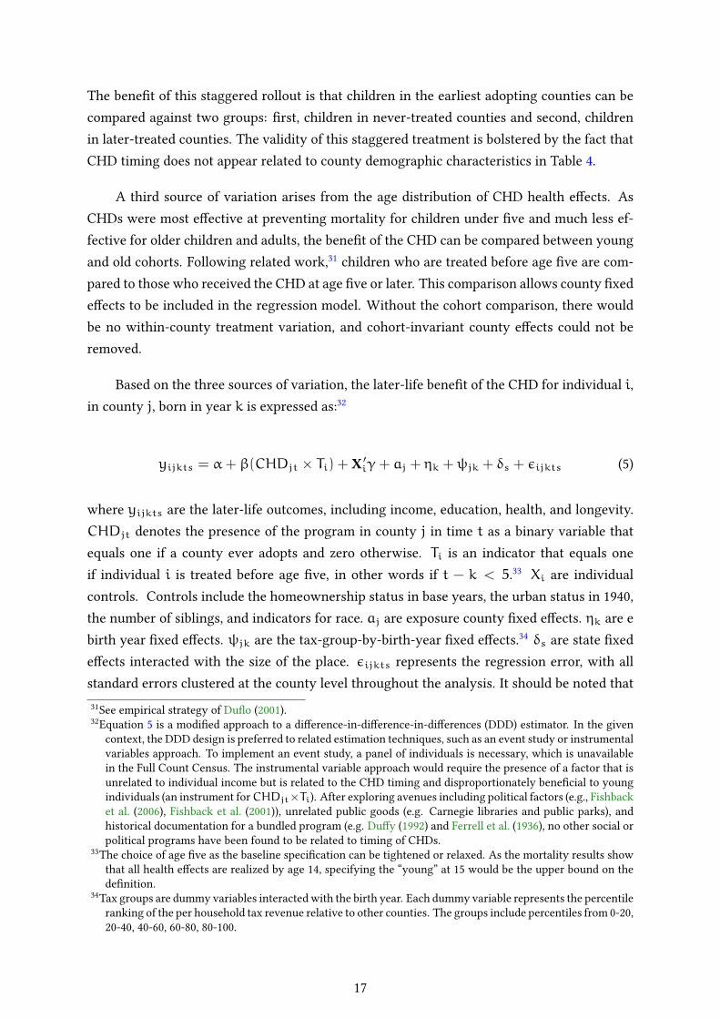
Based on the three sources of variation, the later-life bene�t of the CHD for individual i,in county j, born in year k is expressed as:32

yijkts = α+ β(CHDjt × Ti) + X ′iγ+ aj + ηk +ψjk + δs + εijkts (5)

where yijkts are the later-life outcomes, including income, education, health, and longevity.CHDjt denotes the presence of the program in county j in time t as a binary variable thatequals one if a county ever adopts and zero otherwise. Ti is an indicator that equals oneif individual i is treated before age �ve, in other words if t − k < 5.33 Xi are individualcontrols. Controls include the homeownership status in base years, the urban status in 1940,the number of siblings, and indicators for race. aj are exposure county �xed e�ects. ηk are ebirth year �xed e�ects. ψjk are the tax-group-by-birth-year �xed e�ects.34 δs are state �xede�ects interacted with the size of the place. εijkts represents the regression error, with allstandard errors clustered at the county level throughout the analysis. It should be noted that31See empirical strategy of Du�o (2001).32Equation 5 is a modi�ed approach to a di�erence-in-di�erence-in-di�erences (DDD) estimator. In the given

context, the DDD design is preferred to related estimation techniques, such as an event study or instrumentalvariables approach. To implement an event study, a panel of individuals is necessary, which is unavailablein the Full Count Census. The instrumental variable approach would require the presence of a factor that isunrelated to individual income but is related to the CHD timing and disproportionately bene�cial to youngindividuals (an instrument forCHDjt×Ti). After exploring avenues including political factors (e.g., Fishbacket al. (2006), Fishback et al. (2001)), unrelated public goods (e.g. Carnegie libraries and public parks), andhistorical documentation for a bundled program (e.g. Du�y (1992) and Ferrell et al. (1936), no other social orpolitical programs have been found to be related to timing of CHDs.

33The choice of age �ve as the baseline speci�cation can be tightened or relaxed. As the mortality results showthat all health e�ects are realized by age 14, specifying the “young” at 15 would be the upper bound on thede�nition.

34Tax groups are dummy variables interacted with the birth year. Each dummy variable represents the percentileranking of the per household tax revenue relative to other counties. The groups include percentiles from 0-20,20-40, 40-60, 60-80, 80-100.

17

the �xed e�ect for the timing of implementation, φt, is absorbed by the county �xed e�ectbecause timing does not vary within county.

The advantage of the speci�cation in Equation 5 is the three control groups created forCHDjt×Ti. The �rst group encompasses individuals in the same birth year who are located innever-treated counties, where CHDjt is zero. The second control group includes individualswithin the treated counties but in older cohorts, where Ti is zero. The within-county vari-ation enables the inclusion of county �xed e�ects, aj, which accounts for cohort-invariantunobservable conditions in treated counties. A third control group exists for counties treatedearlier, i.e., before 1925 for the income speci�cation. Children under �ve in early-treatedcounties are compared with children in treated counties (CHDjt is one) who are not exposedunder age �ve (Ti is zero) because they resided in counties that adopted later. As the tim-ing of treatment is unrelated county demographic characteristics, as shown in Table 4, theseindividuals provide an added control for the individuals in early-treated counties. In partic-ular, later-treated individuals help account for unobservable characteristics that may a�ectselection into treatment that are not removed by county �xed e�ects.

Overall, the validity of estimates in Equation 5 rests on two assumptions. The mainassumption is that there are no unobservable county-time e�ects related to instituting a CHD.If the timing of adoption is tied to other public services that a�ect income, such as educationalreforms, the coe�cients will be upward biased. For this to be the case, the unobservableprogram would have to disproportionately bene�t those treated under �ve and be almostperfectly correlated with the timing of the CHD. In e�ect, the secondary program would haveto be bundled with the CHD program while also disproportionately bene�ting those under�ve. In the background historical literature, there is no mention of bundling services withthe CHD rollout.35 Additionally, due to the variation in the adoption decision between statesand the various funding sources that spurred the movement, uniform county-time e�ects areconsidered unlikely.

A secondary assumption of the speci�cation is that younger cohorts experienced greaterhealth bene�ts from CHDs than older cohorts. The mortality e�ects from Section 2.1 form thebasis of this assumption. If this assumption fails, the coe�cients will be biased toward zero,and thus this assumption is less important for the validity of estimates. The magnitude of thedownward bias depends on the relative health bene�ts of younger and older cohorts.36

35See Du�y (1992) and Ferrell et al. (1936).36A rough estimate of the bias could be computed from intuition based on the mortality estimates. In the

mortality results, individuals from �ve to 14 had one death reduced per 1,000 births, while those under �vehad three deaths reduced per 1,000 births. Therefore, the income bene�ts for the young cohorts should bethree times as large as for the older cohorts.

18

5.3 Age of Exposure

To relax the assumption on the de�nition of young and to test whether the precise ageof CHD access impacts long run outcomes, I reconsider the e�ect of the CHD over each yearof childhood, and re-express Equation 5 as:

yijkts = α+

10∑m=0

βm(CHDjt × dim) + X ′iγ+ aj + ηk +ψjk + δs + εijkts (6)

where yijk are the later life outcomes. CHDjt denotes the presence of the program in countyj at time t. dim are indicators for arrival of a CHD at age m, in other words, the di�erencebetween the arrival year and the birth year of each child, t−k = m. Xi are individual controls.aj are birth county �xed e�ects. ηk are age �xed e�ects. ψjk are the tax-group-by-birth-year�xed e�ects. δs are state �xed e�ects interacted with the size of the place. Controls includethe homeownership status in base years, the urban status in 1940, the number of siblings, andindicators for race.

This estimation uses the binary implementation of CHD to measure how health e�ectstransition through childhood. Due to the decline in the mortality response after age �ve, it isexpected that there will be a similar decline over childhood exposure for later-life outcomes.All health e�ects are thought to be realized by age 10, which is why the sum from zero to ageten is chosen.

6 Results

6.1 Baseline E�ect

Table 3 shows the estimated e�ect of CHD exposure on the three measures of adult earn-ings. The results from Equation 5 are consistent across coe�cients; early-life CHD exposureimproves adult earnings.

The central measure of adult earnings, the log of income, is shown in Columns (1)-(4). Inthe full speci�cation with county �xed e�ects, Column (1), children exposed to the CHD whileunder the age of �ve earn almost �ve percent more than control groups. The improvementin annual earnings suggests that children are healthier following treatment with a CHD andthese �tter individuals earn more in adulthood. CHDs are reducing illness scarring in the

19

population (Implication 2), and this decreased disability dominates any mortality selectionpresent (Implication 1).

While annual wages show the direct relationship between health and productivity, betterchildhood health is expected to improve the marginal productivity of each worker. Betterproductivity on the margin will increase earnings for each hour worked as opposed to moretime spent in the labor force. To test productivity, Columns (5)-(8) show the hourly wage. Inthe full speci�cation, Column (5), estimates indicate that CHD exposure leads to a 4.6 percentboost in hourly earnings. The similarity in magnitude to the baseline e�ect suggests thatincome improvements result from higher marginal productivity of individuals rather than atrade-o� between leisure and time spent in the labor force.

To ground the magnitude of income improvement in related public investments, CHDexposure can be compared with the returns to schooling. For the early twentieth century,Clay et al. (2016) �nds that the 1940 return to schooling ranges from 0.064 to 0.079 for 1885-1912 birth cohorts. Thus, the productivity bene�t to CHD treatment is comparable to overone-half of a year of education. This comparison with returns to schooling reveals that thee�ect of the CHD is sizable When considering the relative intensity of each type of investment,the bene�t of the CHD is even more pronounced. Schooling requires the presence of a teacherinteracting with each student daily. Health departments, on the other hand, invested broadly,and possibly once annually in each child. Thus, each CHD generated reasonably high incomereturns when compared to educational investments.

After considering the main results with county �xed e�ects in Columns (1) and (5), I re-place county �xed e�ects with household �xed e�ects to remove time-invariant family charac-teristics. To ensure that only brothers are compared against one another, the sample is limitedto individuals who are sons of the household head in 1920. Columns (2) and (3) show the re-sults from the family �xed e�ects estimation. The coe�cients maintain similar magnitudes tothe county �xed e�ects estimation. Early-life exposure to a health department improves later-life income, even within households. In Column (2), exposed younger brothers show higherannual earnings of 4.8 percent, an e�ect that is slightly larger than the baseline estimate of4.7 percent. For hourly wage, the e�ect declines from 4.6 to 3.9 percent. Utilizing household�xed e�ects gives a somewhat stronger interpretation to the estimates: CHD exposed youngerchildren, as compared with older brothers, are improving their annual earnings. The relativemagnitude resembles the baseline estimates with county �xed e�ects. Furthermore, the com-parative increase in occupational score suggests that younger brothers are moving into higherpaid professions than their older brothers.

In Columns (3) and (4) I perform two initial checks on my baseline estimates. First, Toensure that the e�ect is not entirely driven by migration, I add 1940 county location �xed ef-

20

fects. Now the estimates account for birth-cohort invariant e�ects by county in both 1920 andin 1940. Here the e�ect grows slightly for both the overall wage and hourly wage, which sug-gests that CHD areas and the counties individuals migrate to are disproportionately worse o�.Second, I test county time trends to see if the e�ect is completely driven by wage di�erencesacross cohorts. In Columns (4) and (8) the e�ect dips signi�cantly, but the result maintains itssigni�cance. CHDs are still associated with a wage premium of 1-2 percent after accountingfor county-speci�c trends.

Another initial source of bias could occur if individuals in CHD counties are less likelyto participate in the labor force. This would be especially concerning if lower wages forcedindividuals out of the labor market. I test whether this is the case in Table 4 Column (1).The results are the opposite of expectation, CHD exposed men are more likely to be workingthan non-CHD individuals. This result suggests that actually the bias would be the other wayaround, as individuals who otherwise may not be participating in the labor force, due to lowhuman capital or disability, are now participating in the labor force.

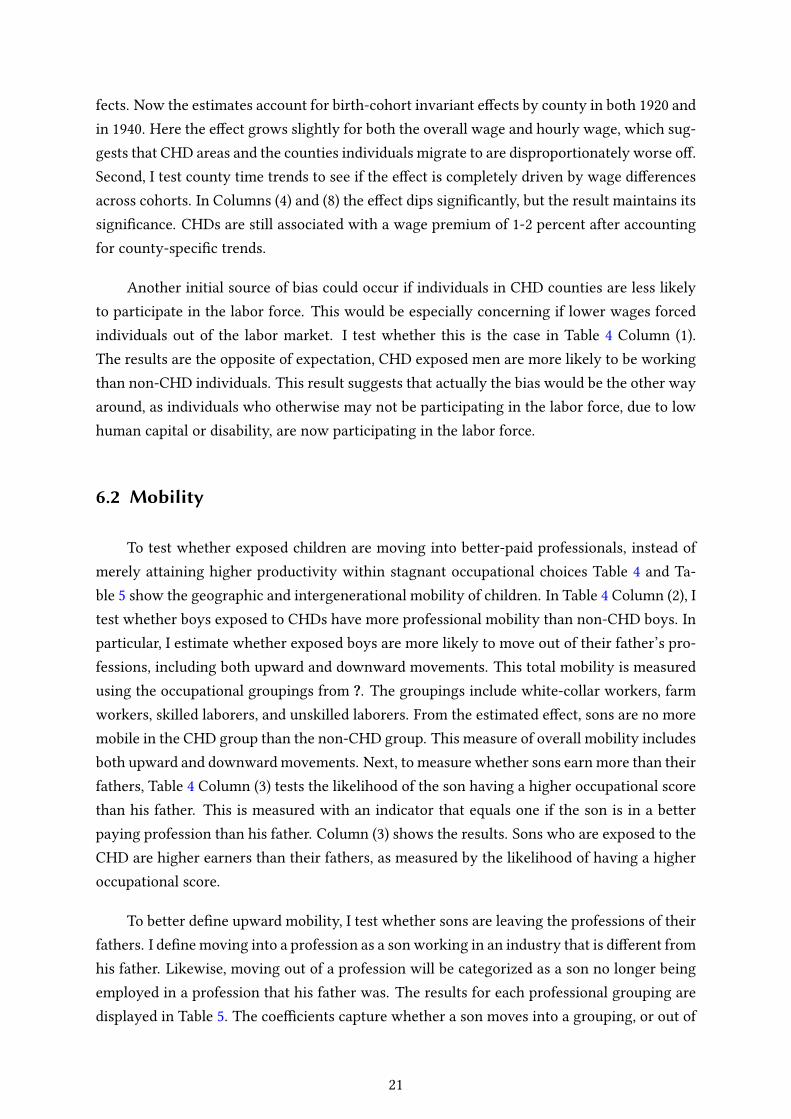
6.2 Mobility

To test whether exposed children are moving into better-paid professionals, instead ofmerely attaining higher productivity within stagnant occupational choices Table 4 and Ta-ble 5 show the geographic and intergenerational mobility of children. In Table 4 Column (2), Itest whether boys exposed to CHDs have more professional mobility than non-CHD boys. Inparticular, I estimate whether exposed boys are more likely to move out of their father’s pro-fessions, including both upward and downward movements. This total mobility is measuredusing the occupational groupings from ?. The groupings include white-collar workers, farmworkers, skilled laborers, and unskilled laborers. From the estimated e�ect, sons are no moremobile in the CHD group than the non-CHD group. This measure of overall mobility includesboth upward and downward movements. Next, to measure whether sons earn more than theirfathers, Table 4 Column (3) tests the likelihood of the son having a higher occupational scorethan his father. This is measured with an indicator that equals one if the son is in a betterpaying profession than his father. Column (3) shows the results. Sons who are exposed to theCHD are higher earners than their fathers, as measured by the likelihood of having a higheroccupational score.

To better de�ne upward mobility, I test whether sons are leaving the professions of theirfathers. I de�ne moving into a profession as a son working in an industry that is di�erent fromhis father. Likewise, moving out of a profession will be categorized as a son no longer beingemployed in a profession that his father was. The results for each professional grouping aredisplayed in Table 5. The coe�cients capture whether a son moves into a grouping, or out of

21

a grouping, based on the above de�nition. With CHD exposure, men are more likely to moveinto white collar professions, less likely to become unskilled laborers, and more likely to moveout of unskilled labor. However, individuals are less likely to move out of farming professionsand more likely to leave skilled labor professions. Since farming professions exclude low skillfarm laborers, this immobility o� farms is not necessarily a negative e�ect. Overall, if it isassumed that unskilled professions are the least preferable, the mobility e�ect of the CHD isbene�cial.

Finally, based on the intergenerational mobility results, it is likely that CHD children maybe more mobile across geographic lines. As occupational mobility often requires migrationbetween states, cities, and counties, healthier sons may be more likely to migrate. The resultsfor migration between states and counties are shown in Columns (4) and (5) of Table 4. CHDexposed children are no more likely to move between states but are more likely to migratefrom one county to another. Individuals appear to be moving into di�erent counties withineach state but are not crossing state lines.

6.3 Age of Exposure

The primary exposure group up to this point has been boys treated before age �ve. Tounderstand how childhood disease exposure impacts lifetime productivity, the assumption onthe age of the e�ect can be relaxed to include the full childhood age distribution (Equation 6).Mapping income gains over childhood provides intuition into exactly when disease exposureis most detrimental when in childhood interventions can be most e�ective.

The CHD e�ect over the age distribution from pre-birth to age ten is shown in Figure V.Exposure that originates in utero yields the highest income boost of 10 percent, with the esti-mated coe�cient declining across the age of introduction to almost disappear by age ten. Thisdeclining e�ect is similar to the reductions in child mortality seen with CHD adoption. Withmortality, infants also were the highest benefactors, with the estimated e�ect on mortalitydeclining through age 14 and disappearing in adulthood. Similarly here, children in infancyand in utero develop the highest bene�t from exposure, with the productivity e�ect decliningthrough childhood. This result implies that the earlier the arrival of health services, the higherthe gains in lifetime earnings.

While the pre-birth indicator may appear to be a falsi�cation test, in actuality, healthdepartments should be more bene�cial if the interventions occur before birth. The basic dis-semination of information on healthy child-rearing, such a breastfeeding, will be most helpfulif the mothers receive it while the children are in utero. Prenatal e�orts, such as examinationsor midwife training, are also most helpful if received before birth. Finally, improved sanitation

22

before conception will improve the mother’s health before pregnancy and result in healthierbabies in utero and at birth. These e�orts will also reduce the likelihood of mothers dying inchildbirth and will bene�t all children in the household.

6.4 Intensive Margin

To test whether the e�ectiveness of the CHD varied based on the investment intensity,I replace the binary treatment indicator with �ve measures of CHD intensity: the share re-ceived from external sources, the budget per capita from general funds, the per capita amountreceived from child initiatives, the number of nurses per 1,000, and the number of inspectorsper 1,000.37 Table 6 displays the estimated coe�cients from Equation 5 across these measuresof intensity. For ease of interpretation, the mean and standard deviation are reported belowthe coe�cients.38

Column (1) shows the fraction of the budget received from external sources. This measureis tested to improve con�dence in the reliability of estimates. As discussed in the identi�cationsection, internal funds are more closely related to the prior income and taxation level of treatedareas. External funding was not related to the disease levels or demographic factors of thecounties involved. Testing external funding boosts con�dence that the �nal e�ect is trulyfrom health improvements and not selection. The coe�cient in Column (1) re�ects a fourpercent increase at the mean level of external funds, with a two percent increase in incomefor each standard deviation above the mean. This result suggests that individuals in countiesthat required more external funding bene�ted more than those in counties that put up fundsfrom internal budgets. This may be due to needy individuals receiving external funds, butthere is no evidence for this based on the selection into treatment. Nonetheless, estimateshere help to boost con�dence in the baseline e�ect, as the external funds are quasi-random.

Column (2) presents the e�ect of increasing the intensity of the CHD through the bud-get per capita. The results show little e�ect with the coe�cient near zero and insigni�cant.CHDs were given a target budget per capita, and therefore, had little variation per capita intheir total budget. This �xed budget helps to explain the lack of e�ect over the per capitaspending. In Column (3), the child health funding per capita shows a more interesting result.Counties that received more per capita from child health initiatives had higher bene�ts fromthe CHD. This result as compared with the estimated e�ect for budget per capita shows thatthe funding initiative for each health department did matter. Areas receiving child healthfunds tailored their focus to health services, which in turn, generated higher income e�ects.

37General funds include all funds not targeted towards children, county, state, USPHS, and other funding sources.Child funds include mother-infant funds and RSC donations.

38The reported summary statistics are calculated only in areas with a CHD.

23

This helps to con�rm the intuition that child health e�ects are the main mechanism for theincome improvements.

Finally, the nurses and inspectors per 1,000 individuals are shown in Columns (4) and (5).Both sta� types show similar e�ects at the mean, around a percentage increase in income. Thebene�t from hiring inspectors increases by more at each standard deviation above the mean.For a county that hires more inspectors than the average, the income gains would go up by2.4 percent for each standard deviation above the mean. For nurses, the e�ect would onlyincrease by 2.0 percent. This higher bene�t from inspectors suggests that either there was anincreasing bene�t from better sanitation measures or that more e�ective departments realizedthat sanitation was an important function of CHD. Either way, increasing the intensity of thesta� members increases the bene�t for individuals in the county.

7 Channels

To unravel the channels by which declining morbidity and mortality improve earnings Iconsider the adult education and health of exposed children. Educational outcomes originatefrom the census, while health measures are drawn from the WWII enlistment data and theSocial Security Death Master File. Based on the income results and Implications 1-5, both edu-cational outcomes and adult health are expected to improve with enhancements in childhoodhealth.

7.1 Education

Children who are healthier as a result of exposure to CHDs may show an increase ineither the quantity or quality of schooling. Healthier children, with lower levels of disability,should perform better in school. This better performance should then increase the quantity ofschooling attained due to higher returns over each additional year of schooling. This increasedhuman capital investment through education would then lead to higher lifetime earnings.

Focusing on the years of schooling, based on Implication 4, exposed children will increasetheir educational investment if healthier children have higher returns to education. In otherwords, if children previously experienced disability or health issues that a�ected their abilityto bene�t from schooling, then CHD exposure should increase total educational attainment.Column (1) of Table 7 in Panel A display the results for the binary implementation of Equa-tion 5 on the terminal year of education. The estimated e�ect reveals that CHD exposuredoes not a�ect the total years of schooling. Individuals do not appear to be adjusting their

24

total investment in education based on improved health. This result contradicts the initialexpectation and may be due to several factors, including the low returns to education in ruralareas.

To test whether individuals are investing di�erently over the years of schooling, I con-sider whether students alter their terminal degree level, instead of their total years of school-ing. The results for the likelihood of graduating from both eighth grade and high school areshown in Columns (2) and (3). CHD exposed children are less likely to graduate from highschool than comparison cohorts. Simultaneously, there appears to be a small positive e�ect onthe likelihood of graduating from eighth grade. Here the educational changes are bene�tingthe lower end of the distribution, with individuals graduating from eighth grade at a higherrate. These same individuals, however, are failing to increase their high school graduationrates. Two possible explanations for this shift exist. First, the return to a high school degreemay be relatively low in rural areas, which implies that the decline in graduation results froma weak incentive to invest in a terminal high school degree. Second, as improved health raisesthe productivity of a�ected individuals, children may be leaving school early to take advan-tage of the wage bene�ts from higher productivity. These two explanations could combine ina way that would incentivize individuals to leave school earlier with better health.

After �nding no e�ect on total years of schooling, I consider whether CHDs a�ected thequality of education. Unfortunately, the 1940 census does not report literacy or writing ability,and instead an alternative measure of schooling quality must be used. Grade regression, orhow far behind from the correct grade level a student is, provides an alternative measure ofin-school productivity. The intuition behind this measure is that children who miss less schoolare more likely to keep up in classes and maintain the appropriate grade level for their age.An example of grade regression is noted in the documentation surrounding the CHD:

The whole-time district health o�cer, in the course of his �rst round of physical examination of

school children, found, in October, 1919, at one of the large graded schools, 16 pupils of widely

di�erent ages who, because they were unable to keep up with their respective classes, were re-

garded as mentally backward and were assigned to a special room for simple instructions. Upon

carefully examining the 16 children, the health o�cer found that every one had one or more

marked physical defects, among which decayed teeth, enlarged tonsils, adenoids, faulty eye-

sight, and poor hearing were common. With the cooperation of the school directors, the health

o�cer, within the next few months, by appeals to the parents and through special arrange-

ments with local physicians, succeeded in having corrected almost all of the physical defects

found among the group. On reexamination of the pupils a year later, it was found that all of

the previously backward children had been returned to their proper grades and were keeping

up in them with their classmates. (?, 1922 p. 2369)

25

To test whether CHDs decreased the probability of children being behind in school, esti-mation considers the number of grades behind from the age-appropriate level a child is.39 Theresults are shown in Panel B. The main e�ect in Column (1) is a reduction in grade regressionby 0.098 or about a month of schooling. Thus, results con�rm the anecdotal evidence andshow that individuals exposed to the CHD are less likely to fall behind in classes and moreable to complete their education at the correct age. The improved health of children bene�tstheir performance in school and occurs despite the stagnant quantity of education.40

In Columns (2) and (3), the estimation tests whether CHDs a�ect the likelihood of boysworking or being enrolled in school. With lower grade regression, individuals may �nishschool more quickly and enter the labor force earlier. This earlier labor force participationcould explain a portion of the income gains through more work experience at each age. Hereresults appear to show a slight reduction in the likelihood of being enrolled in school butno increased likelihood of working full-time. Thus, it does not appear that individuals areentering the labor force earlier with reduced grade regression. While children are less likelyto be enrolled in school, they do not appear more likely to enter the labor force.

7.2 Health and Cognitive Scores

Turning to the health measures available in the World War II Enlistment Records, both thebody mass index (BMI) and the cognitive scores of enlisted men are considered. Health e�ectsare tested to distinguish between the contrasting e�ect of decreased mortality selection andthe lower morbidity levels in the population (Implications 1 and 2). World War II records havethe added bene�t of being collected by an objective third party, instead of the self-reportedmeasures collected by the census.

Table 8 shows the results for BMI and height. In Column (3), men exposed to the CHDshow an increase in BMI relative to control groups. While from a contemporary perspectivean increase in BMI signals poor health, during the 1940s underweight and malnourished menwere more common than obese men.41 Most of the health concerns of the day surroundedundernourishment rather than obesity. This also means, however, that the worst cases ofmalnourished men were rejected from enlistment and the data is bottom censored. A 1942NewYork Times article discussing the stature of rejected men notes that "the number of youths who

39Grade regression is de�ned as the number of years away from the age-appropriate grade level. Age appropriategrade level begins at year one of education, when the individuals should be six or seven years old. Year twoof education is when the individual should be seven or eight years old and so on until the child is 18 yearsof age.

40Grade regression results should be interpreted with caution as the grade level su�ers from measurement issuesdue to ungraded schools, which is especially true in Southern states. For further explanation on the issue,see ? and ?.

41See Grumstrup-Scott et al. (1992)

26

are soft, underweight and generally lacking in muscular development is very large" (Davis(1942)) and as many as 45 percent of men were rejected from service. The direction of the biascreated from the selection of healthier recruits depends on the county-level composition ofrejected individuals. Unfortunately, I have not found a way to gather information on rejectedmen.

Height in Column (1) tells a di�erent story than the BMI. Men who are exposed to theCHD are slightly shorter than untreated men. This result points to some level of reduced mor-tality selection in the population. While children who survive may have less scarring overall,they still retain evidence of worse health. The lower height of exposed children suggests thatthere may be a trade-o� between mortality selection and lower morbidity in the population.The selection dominating e�ect in height is likely due to the high initial mortality conditionsat the time. Similar �ndings by Bozzoli et al. (2009) have shown that, at high mortality levels,selection will dominate scarring. While the e�ect here is small, the reduction in height revealsthe complex relationship between disease and later-life health.

Finally, considering cognition in Columns (4) men exposed to the CHD while under theage of �ve fail to show an improvement in cognition. While the coe�cient is positive, thee�ect is not signi�cant. The smaller sample size may be driving this result, but it is di�cultto determine.

7.3 Longevity

I next consider whether CHDs a�ected the lifespan of adults using the Social SecurityDeath Master File. Matching this data to the 1930 census, I �nd that CHDs did not a�ectthe lifespan of exposed individuals. Instead, CHDs increased the likelihood that individualswould live into their 80s and 90s but decreased the probability of men living past age 60. This�nding corroborates the perceived presence of mortality selection in the population. Fromboth the results here and the results with height, at the tail end of the distribution individualswith lower levels of health survive into adulthood. The diminished probability of reachingage 60 suggests that exposed children manage to live into adulthood but still die earlier thancontrol groups. CHDs, however, appear to bene�t healthier men, as exposure increases thelikelihood that individuals live past age 80. These estimates are shown in Table 8, for theoverall longevity, and the probability of living past each age, 60, 70, and 80. At the top endof the longevity distribution, exposed men live longer, but at the tail end, exposed men haveshorter lifespans.

These results suggest that CHDs helped the healthiest men to attain better health whileallowing sicker men to survive into adulthood. This corroborates �ndings from the WWII

27

enlistment records. Over all measures of health, exposure produces higher BMI and the prob-ability of living past age 80 but lowers adult height and the probability of living to age 60.Put together, the results suggest that exposure leads to both decreasing morbidity and lowermortality.

8 Robustness

8.1 Program E�ect with Young Adult Exposure

A fundamental assumption in Equations 5 and 6 is that children under the age of �veexperience the highest bene�ts from CHDs. Since health e�ects are large in infancy anddecline into adulthood, the income pattern is expected to be similar. CHDs should be lessadvantageous for adults or older children. To test whether children under �ve are the onlybene�ciaries of the CHD program, I test di�erent exposure cohorts. As opposed to the expo-sure group as under age of �ve, I check whether older age groups bene�ted from the program.The age groups I select include: before age 5, ages 5 to 10, ages 10 to 15, and ages 15 to 20.

Table 9 Panel A Column (2) presents those exposed between 10 and 15 who are 30 to 49,in 1940. Similarly, Column (3) tests exposure between 15 and 20 for those 35 to 49, and so onfor Column (4). Across Table 9 Columns (1)-(4), older children and young adults are eithernegatively a�ected or not a�ected by CHD exposure. The lack of e�ect in adulthood is thesame as noted under the mortality bene�ts of CHDs. Results here strengthen con�dence inthe chosen speci�cation and the baseline results.42

8.2 Changing Life-cycle of Income

Identi�cation further rests on the supposition that the life-cycle earnings pattern areconstant within each county and over time. If there are unobservable cohort-speci�c wagepatterns the control groups would be a poor comparison for the exposed individuals. Myinitial test on this included county-speci�c time trends which did not eliminate the e�ect.To further ensure that cohort-speci�c wage patters are not driving the main result I performthree additional tests.

First, I limit the exposure window for the older cohorts. The smaller exposure windowcompares those who received a CHD before age �ve with those who just missed the cuto�

42Results in Column (1) are lower than baseline because the comparison group is limited to under �ve versusthe cohort aged �ve to 10.

28

age and were �ve and ten when the CHD opened. This restricted comparison bounds thedivergence in life-cycle income between cohorts. Table 9 Panel A Column (1) displays theresults from Table 3 iwith the cohort restriction. Column (1) shows the e�ect with the com-parison older cohort limited to ages �ve through ten. The estimated e�ect on this restrictedsample is comparable to the baseline estimates in Table 3. There is a 0.04 percent decline inthe estimated coe�cient, but the e�ect is still near four percent. This coe�cient shows that,even with the restricted age range, exposed cohorts still maintain a substantial e�ect, whichalleviates concern over divergence in life-cycle income patterns.

Second, I utilize the log of the occupational score. The log of occupational score measuresthe median wage by occupation and removes cohort-speci�c earnings patterns. Instead, occu-pation score tests whether individuals are moving between professions with CHD exposure.Columns (5) and (6) display the results with the occupational score. The full speci�cation withthe original sample and county �xed e�ects is shown in Column (6). CHD exposure resultsin a 1.9 percent increase in the occupational score when compared with control groups. Test-ing the median income by profession removes within-occupation income variation, and thedecline in e�ect is expected. The drop occurs because the log of occupational score only cap-tures between-profession di�erences. The smaller estimate suggests that within-occupationvariability in income is accounting for half of the earnings boost, while occupation mobility isgenerating the remainder of the e�ect. While the e�ect is lower than the baseline estimates,the use of the occupational standing creates a lower bound on the estimates and removes con-cern over inter-life-cycle income di�erences driving the full e�ect. In addition to the sampleof individuals reporting income, I also test the full sample of occupation score. In Column(5) the e�ect is muted as compared to Column (6). The income bene�t is lower for the fullsample of individuals as opposed to those who continuous wage. This result suggests that thebaseline e�ect may be slightly overstated due to non-wage earners in the sample.

Next, I limit the age window of the sample to an upper bound of age 30 and 35. Initially,the upper bound of 39 is chosen to encompass all treated individuals. Instead, I limit thesample to men between 18 and 31 as well as 18 to 36. Table 9 Panel B Columns (1)-(2) showthe results with the lower age ceiling. For those who are 19 to 30, the income gain is nowestimated at three percent and represents a smaller improvement than the baseline e�ect of�ve percent. For those who are 18 to 36, the bene�t is 3.8 percent. Through both adjustmentsto the speci�cation, the coe�cient remains between three and four percent and signi�cant.The decline in magnitude is likely due to the loss of �rst treated individuals as well as earlycontrol groups for treated counties.

29

8.3 Excluding Higher Education

Next, I exclude individuals with higher levels of education to address three concerns.First, higher returns to education may be in�ating the e�ect for younger cohorts. Second,individuals who graduate from college may be underrepresented in the 19 to 39 sample. Third,the average could be in�ated by a small number of high-achieving men with better educationlevels. To alleviate these concerns, I exclude individuals who graduate from college and highschool from the sample.

The �rst two columns of Table 9 Panel B show the estimates excluding individuals withhigher levels of schooling, speci�cally those who graduate from high school and college. Col-umn (3) shows estimates excluding high school graduates. The e�ect declines by 0.2 percentfrom the baseline. Despite this drop, the CHD results in a 4.5 percent income boost. The e�ectis similar in Column (4) in the sample without college graduates. The results without highschool and college graduates suggest that the earnings increase is mainly a�ecting those atthe lower end of the income distribution. This corroborates earlier education results, whereindividuals were more likely to graduate from eighth grade but less likely to graduate fromhigh school.

8.4 Adjusted Age Linking

The baseline linked sample includes individuals whose mismatch in age by as many asthree years and may generate concern that the sample contains mislinked men. To accommo-date this concern, I re-estimate results over a restricted sample and only include individualswho di�er in age by no more than one and two years. Table 9 Panel B shows the results.Column (5) contains individuals who di�er in age by no more than one year, and Column(6) presents the sample of men who match within two years. Across Column (5) there is aslight dip in e�ect, where exposure results in a 4.3 percent income boost. Column (6) showsno di�erence from the baseline e�ect.

8.5 Additional Controls

The baseline speci�cation employs �xed e�ects for the year of birth, county of birth, andthe number of siblings, and the home ownership status. To test whether additional controlsalter the outcome the original speci�cation, I add controls for the number of years of schoolingand the 1920 household income.

30

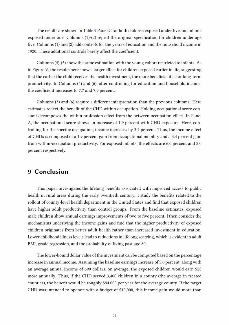
The results are shown in Table 9 Panel C for both children exposed under �ve and infantsexposed under one. Columns (1)-(2) repeat the original speci�cation for children under age�ve. Columns (1) and (2) add controls for the years of education and the household income in1920. These additional controls barely a�ect the coe�cient.

Columns (4)-(5) show the same estimation with the young cohort restricted to infants. Asin Figure V, the results here show a larger e�ect for children exposed earlier in life, suggestingthat the earlier the child receives the health investment, the more bene�cial it is for long-termproductivity. In Columns (5) and (6), after controlling for education and household income,the coe�cient increases to 7.7 and 7.9 percent.

Columns (3) and (6) require a di�erent interpretation than the previous columns. Hereestimates re�ect the bene�t of the CHD within occupation. Holding occupational score con-stant decomposes the within profession e�ect from the between occupation e�ect. In PanelA, the occupational score shows an increase of 1.9 percent with CHD exposure. Here, con-trolling for the speci�c occupation, income increases by 3.4 percent. Thus, the income e�ectof CHDs is composed of a 1.9 percent gain from occupational mobility and a 3.4 percent gainfrom within-occupation productivity. For exposed infants, the e�ects are 6.0 percent and 2.0percent respectively.

9 Conclusion

This paper investigates the lifelong bene�ts associated with improved access to publichealth in rural areas during the early twentieth century. I study the bene�ts related to therollout of county-level health department in the United States and �nd that exposed childrenhave higher adult productivity than control groups. From the baseline estimates, exposedmale children show annual earnings improvements of two to �ve percent. I then consider themechanisms underlying the income gains and �nd that the higher productivity of exposedchildren originates from better adult health rather than increased investment in education.Lower childhood illness levels lead to reductions in lifelong scarring, which is evident in adultBMI, grade regression, and the probability of living past age 80.

The lower-bound dollar value of the investment can be computed based on the percentageincrease in annual income. Assuming the baseline earnings increase of 5.0 percent, along withan average annual income of 690 dollars, on average, the exposed children would earn $28more annually. Thus, if the CHD served 3,400 children in a county (the average in treatedcounties), the bene�t would be roughly $94,000 per year for the average county. If the targetCHD was intended to operate with a budget of $10,000, this income gain would more than

31

cover the expected cost. This estimate, however, cannot capture the full bene�t to exposedindividuals through better overall health, fewer illness episodes, and a reduced probability ofdying early. Thus, the raw income calculations underestimate the impact on individual utilityand societal welfare.

To understand how such health investments should be prioritized relative to other publicinterventions, the CHD cost can be compared with parallel infrastructure investments of theperiod. In the historical literature, it is noted that "the money spent for 1 mile of paved roadwould buy adequate health service for three of the counties for a year" (?, 1926 pp 2413). Thus,health services were a relatively small cost, compared with the infrastructure investments thatcoincided with the movement. When considering the income bene�ts for the residents, therelatively small initial cost is o�set by the future increase in taxable base.

Finally, it is informative to consider the complementaries of improved health with pub-lic investment in schooling. If poor child health diminishes the returns to schooling, thensolely prioritizing educational investments makes little sense. The historical literature drawsthis comparison and notes that the poor health of rural children ensured that "the e�ciencyof the public-school system is necessarily low, and it seems certain that by diverting to e�-cient public-health work some of the money appropriated for schools-even to the extent, ifnecessary, of causing all the public schools to be closed for one year in �ve-a net gain couldbe realized in the speci�cally educational results from the public-school system" (?, 1926 pp2413). Thus, the bene�t of investing CHDs complemented the schooling improvements ofthe period. This complementarity was to the degree that it even made sense to close publicschools, for a time, to pay for the health investment.

Overall, this paper quanti�es the bene�t associated with local health initiatives that tar-get childhood illnesses and sanitation. The lasting improvements for individuals in term ofhealth and productivity provide evidence for the necessity of targeted health investments inrural areas today. The direct relationship between health and income motivates similar pro-grams to mitigate preventable illnesses in both developed and developing areas of the world.The rural section of developing countries, in particular, continue to struggle with many of thediseases that plagued the US during the early 20th century.

32

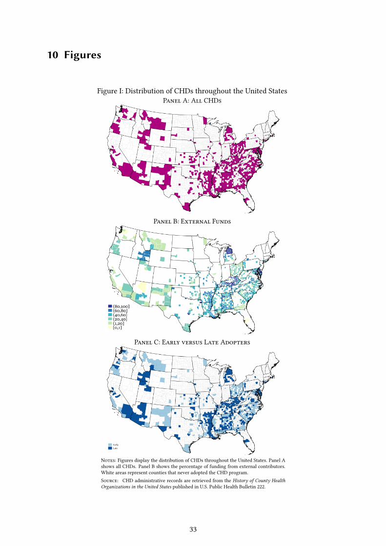
10 Figures

Figure I: Distribution of CHDs throughout the United StatesPanel A: All CHDs

Panel B: External Funds

Panel C: Early versus Late Adopters

Notes: Figures display the distribution of CHDs throughout the United States. Panel Ashows all CHDs. Panel B shows the percentage of funding from external contributors.White areas represent counties that never adopted the CHD program.Source: CHD administrative records are retrieved from the History of County HealthOrganizations in the United States published in U.S. Public Health Bulletin 222.

33

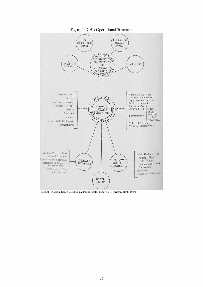
Figure II: CHD Operational Structure

Source: Diagram from State Biennial Public Health Reports of Tennessee (1926-1929).

34

Figure III: Example CHD Activities

Source: Examples from State Biennial Public Health Reports of Tennessee (1926-1929).

35

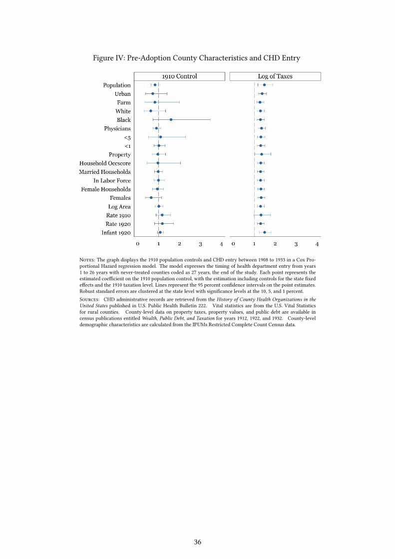
Figure IV: Pre-Adoption County Characteristics and CHD Entry

Notes: The graph displays the 1910 population controls and CHD entry between 1908 to 1933 in a Cox Pro-portional Hazard regression model. The model expresses the timing of health department entry from years1 to 26 years with never-treated counties coded as 27 years, the end of the study. Each point represents theestimated coe�cient on the 1910 population control, with the estimation including controls for the state �xede�ects and the 1910 taxation level. Lines represent the 95 percent con�dence intervals on the point estimates.Robust standard errors are clustered at the state level with signi�cance levels at the 10, 5, and 1 percent.Sources: CHD administrative records are retrieved from the History of County Health Organizations in theUnited States published in U.S. Public Health Bulletin 222. Vital statistics are from the U.S. Vital Statisticsfor rural counties. County-level data on property taxes, property values, and public debt are available incensus publications entitled Wealth, Public Debt, and Taxation for years 1912, 1922, and 1932. County-leveldemographic characteristics are calculated from the IPUMs Restricted Complete Count Census data.

36

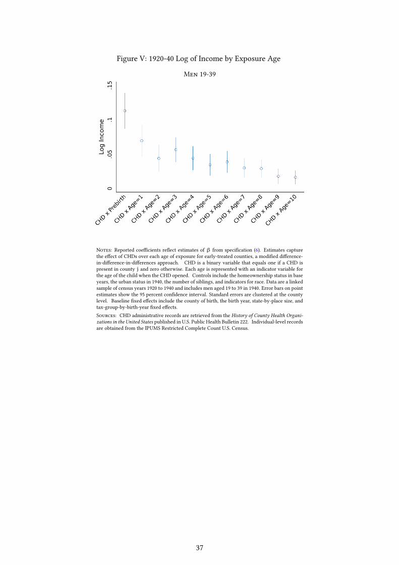
Figure V: 1920-40 Log of Income by Exposure Age

Men 19-39

Notes: Reported coe�cients re�ect estimates of β from speci�cation (6). Estimates capturethe e�ect of CHDs over each age of exposure for early-treated counties, a modi�ed di�erence-in-di�erence-in-di�erences approach. CHD is a binary variable that equals one if a CHD ispresent in county j and zero otherwise. Each age is represented with an indicator variable forthe age of the child when the CHD opened. Controls include the homeownership status in baseyears, the urban status in 1940, the number of siblings, and indicators for race. Data are a linkedsample of census years 1920 to 1940 and includes men aged 19 to 39 in 1940. Error bars on pointestimates show the 95 percent con�dence interval. Standard errors are clustered at the countylevel. Baseline �xed e�ects include the county of birth, the birth year, state-by-place size, andtax-group-by-birth-year �xed e�ects.Sources: CHD administrative records are retrieved from the History of County Health Organi-zations in the United States published in U.S. Public Health Bulletin 222. Individual-level recordsare obtained from the IPUMS Restricted Complete Count U.S. Census.

37

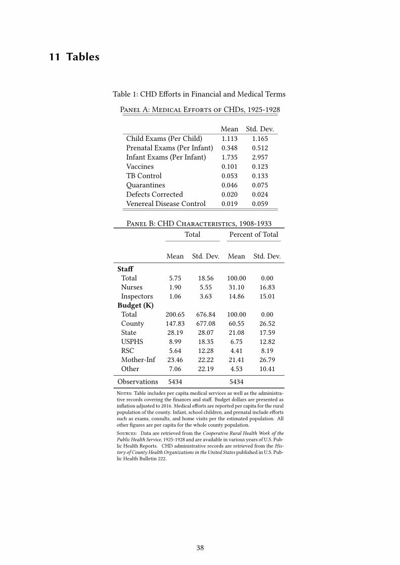
11 Tables

Table 1: CHD E�orts in Financial and Medical Terms

Panel A: Medical Efforts of CHDs, 1925-1928

Mean Std. Dev.Child Exams (Per Child) 1.113 1.165Prenatal Exams (Per Infant) 0.348 0.512Infant Exams (Per Infant) 1.735 2.957Vaccines 0.101 0.123TB Control 0.053 0.133Quarantines 0.046 0.075Defects Corrected 0.020 0.024Venereal Disease Control 0.019 0.059

Panel B: CHD Characteristics, 1908-1933Total Percent of Total

Mean Std. Dev. Mean Std. Dev.

Sta�Total 5.75 18.56 100.00 0.00Nurses 1.90 5.55 31.10 16.83Inspectors 1.06 3.63 14.86 15.01Budget (K)Total 200.65 676.84 100.00 0.00County 147.83 677.08 60.55 26.52State 28.19 28.07 21.08 17.59USPHS 8.99 18.35 6.75 12.82RSC 5.64 12.28 4.41 8.19Mother-Inf 23.46 22.22 21.41 26.79Other 7.06 22.19 4.53 10.41

Observations 5434 5434Notes: Table includes per capita medical services as well as the administra-tive records covering the �nances and sta�. Budget dollars are presented asin�ation adjusted to 2016. Medical e�orts are reported per capita for the ruralpopulation of the county. Infant, school children, and prenatal include e�ortssuch as exams, consults, and home visits per the estimated population. Allother �gures are per capita for the whole county population.Sources: Data are retrieved from the Cooperative Rural Health Work of thePublic Health Service, 1925-1928 and are available in various years of U.S. Pub-lic Health Reports. CHD administrative records are retrieved from the His-tory of County Health Organizations in the United States published in U.S. Pub-lic Health Bulletin 222.

38

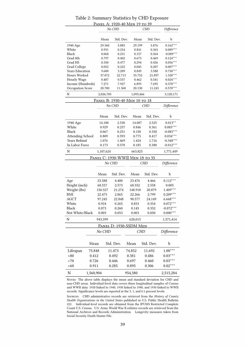
Table 2: Summary Statistics by CHD ExposurePanel A: 1920-40 Men 19 to 39

No CHD CHD Di�erence

Mean Std. Dev. Mean Std. Dev. b

1940 Age 29.360 5.885 29.199 5.876 0.162∗∗∗White 0.931 0.254 0.841 0.365 0.089∗∗∗Black 0.068 0.251 0.157 0.364 -0.089∗∗∗Grad 8th 0.797 0.402 0.673 0.469 0.124∗∗∗Grad HS 0.350 0.477 0.294 0.456 0.056∗∗∗Grad College 0.052 0.222 0.045 0.207 0.007∗∗∗Years Education 9.600 3.209 8.849 3.588 0.750∗∗∗Hours Worked 37.072 22.713 35.752 21.897 1.320∗∗∗Hourly Wage 0.487 0.537 0.462 0.541 0.024∗∗∗Income (Hundreds) 7.271 7.927 6.893 7.695 0.378∗∗∗Occupation Score 20.700 11.368 20.130 11.243 0.570∗∗∗

N 2,026,705 1,093,466 3,120,171

Panel B: 1930-40 Men 10 to 18No CHD CHD Di�erence

Mean Std. Dev. Mean Std. Dev. b

1940 Age 14.100 2.530 14.087 2.525 0.013∗∗White 0.929 0.257 0.846 0.361 0.083∗∗∗Black 0.067 0.251 0.150 0.358 -0.083∗∗∗Attending School 0.809 0.393 0.775 0.417 0.034∗∗∗Years Behind 1.076 1.469 1.424 1.716 -0.348∗∗∗In Labor Force 0.173 0.378 0.185 0.388 -0.012∗∗∗

N 1,107,624 663,825 1,771,449

Panel C: 1930-WWII Men 18 to 35No CHD CHD Di�erence

Mean Std. Dev. Mean Std. Dev. b

Age 23.588 4.480 23.476 4.466 0.112∗∗∗Height (inch) 68.557 2.573 68.552 2.558 0.005Weight (lbs) 150.327 21.274 148.918 20.879 1.409∗∗∗BMI 22.475 2.865 22.266 2.799 0.209∗∗∗AGCT 97.245 22.848 90.577 24.149 6.668∗∗∗White 0.924 0.265 0.853 0.354 0.072∗∗∗Black 0.073 0.260 0.145 0.352 -0.072∗∗∗Not White/Black 0.003 0.053 0.003 0.050 0.000∗∗∗

N 943,399 628,015 1,571,414

Panel D: 1930-SSDM MenNo CHD CHD Di�erence

Mean Std. Dev. Mean Std. Dev. b

Lifespan 75.848 11.473 74.852 11.692 1.00∗∗∗>80 0.412 0.492 0.381 0.486 0.03∗∗∗>70 0.726 0.446 0.697 0.460 0.03∗∗∗>60 0.911 0.285 0.895 0.306 0.02∗∗∗

N 1,560,904 954,380 2,515,284Notes: The above table displays the mean and standard deviation for CHD andnon-CHD areas. Individual-level data covers three longitudinal samples of Censusand WWII data: 1920 linked to 1940, 1930 linked to 1940, and 1930 linked to WWIIrecords. Signi�cance levels are reported at the 5, 1, and 0.1 percent levels.Sources: CHD administrative records are retrieved from the History of CountyHealth Organizations in the United States published in U.S. Public Health Bulletin222. Individual-level records are obtained from the IPUMS Restricted CompleteCount U.S. Census. U.S. Army World War II enlistee records are retrieved from theNational Archives and Records Administration. Longevity measures taken fromSocial Security Death Master File.

39

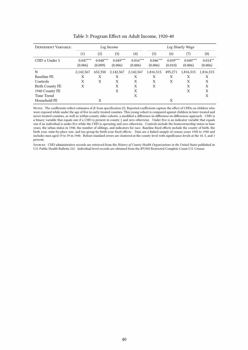
Table 3: Program E�ect on Adult Income, 1920-40

Dependent Variable: Log Income Log Hourly Wage

(1) (2) (3) (4) (5) (6) (7) (8)

CHD x Under 5 0.047*** 0.048*** 0.049*** 0.016*** 0.046*** 0.039*** 0.049*** 0.014**(0.006) (0.009) (0.006) (0.006) (0.006) (0.010) (0.006) (0.006)

N 2,142,567 652,350 2,142,567 2,142,567 1,816,515 495,271 1,816,515 1,816,515Baseline FE X X X X X X X XControls X X X X X X X XBirth County FE X X X X X X1940 County FE X X X XTime Trend X XHousehold FE X X

Notes: The coe�cients re�ect estimates ofβ from speci�cation (5). Reported coe�cients capture the e�ect of CHDs on children whowere exposed while under the age of �ve in early-treated counties. This young cohort is compared against children in later-treated andnever-treated counties, as well as within-county older cohorts, a modi�ed a di�erence-in-di�erence-in-di�erences approach. CHD isa binary variable that equals one if a CHD is present in county j and zero otherwise. Under �ve is an indicator variable that equalsone if an individual is under �ve while the CHD is operating and zero otherwise. Controls include the homeownership status in baseyears, the urban status in 1940, the number of siblings, and indicators for race. Baseline �xed e�ects include the county of birth, thebirth year, state-by-place size, and tax-group-by-birth-year �xed e�ects. Data are a linked sample of census years 1920 to 1940 andincludes men aged 19 to 39 in 1940. Robust standard errors are clustered at the county level with signi�cance levels at the 10, 5, and 1percent.Sources: CHD administrative records are retrieved from the History of County Health Organizations in the United States published inU.S. Public Health Bulletin 222. Individual-level records are obtained from the IPUMS Restricted Complete Count U.S. Census.

40

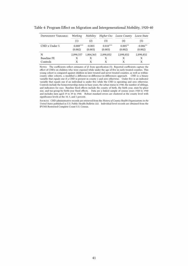
Table 4: Program E�ect on Migration and Intergenerational Mobility, 1920-40

Dependent Variable: Working Mobility Higher Occ Leave County Leave State

(1) (2) (3) (4) (5)

CHD x Under 5 0.008*** -0.003 0.010*** 0.005** -0.006**(0.002) (0.003) (0.003) (0.002) (0.002)

N 2,890,557 1,804,365 2,890,852 2,890,852 2,890,852Baseline FE X X X X XControls X X X X X

Notes: The coe�cients re�ect estimates of β from speci�cation (5). Reported coe�cients capture thee�ect of CHDs on children who were exposed while under the age of �ve in early-treated counties. Thisyoung cohort is compared against children in later-treated and never-treated counties, as well as within-county older cohorts, a modi�ed a di�erence-in-di�erence-in-di�erences approach. CHD is a binaryvariable that equals one if a CHD is present in county j and zero otherwise. Under �ve is an indicatorvariable that equals one if an individual is under �ve while the CHD is operating and zero otherwise.Controls include the homeownership status in base years, the urban status in 1940, the number of siblings,and indicators for race. Baseline �xed e�ects include the county of birth, the birth year, state-by-placesize, and tax-group-by-birth-year �xed e�ects. Data are a linked sample of census years 1920 to 1940and includes men aged 19 to 39 in 1940. Robust standard errors are clustered at the county level withsigni�cance levels at the 10, 5, and 1 percent.Sources: CHD administrative records are retrieved from the History of County Health Organizations in theUnited States published in U.S. Public Health Bulletin 222. Individual-level records are obtained from theIPUMS Restricted Complete Count U.S. Census.

41

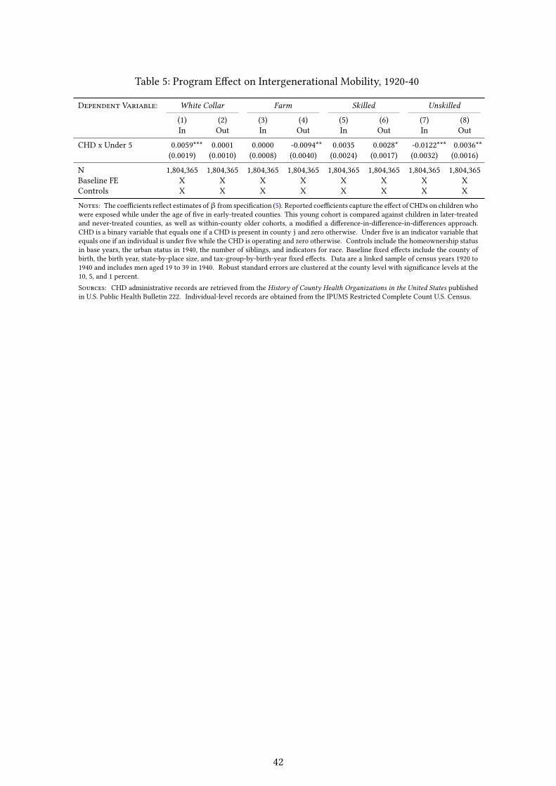
Table 5: Program E�ect on Intergenerational Mobility, 1920-40

Dependent Variable: White Collar Farm Skilled Unskilled

(1) (2) (3) (4) (5) (6) (7) (8)In Out In Out In Out In Out

CHD x Under 5 0.0059*** 0.0001 0.0000 -0.0094** 0.0035 0.0028* -0.0122*** 0.0036**(0.0019) (0.0010) (0.0008) (0.0040) (0.0024) (0.0017) (0.0032) (0.0016)

N 1,804,365 1,804,365 1,804,365 1,804,365 1,804,365 1,804,365 1,804,365 1,804,365Baseline FE X X X X X X X XControls X X X X X X X X

Notes: The coe�cients re�ect estimates ofβ from speci�cation (5). Reported coe�cients capture the e�ect of CHDs on children whowere exposed while under the age of �ve in early-treated counties. This young cohort is compared against children in later-treatedand never-treated counties, as well as within-county older cohorts, a modi�ed a di�erence-in-di�erence-in-di�erences approach.CHD is a binary variable that equals one if a CHD is present in county j and zero otherwise. Under �ve is an indicator variable thatequals one if an individual is under �ve while the CHD is operating and zero otherwise. Controls include the homeownership statusin base years, the urban status in 1940, the number of siblings, and indicators for race. Baseline �xed e�ects include the county ofbirth, the birth year, state-by-place size, and tax-group-by-birth-year �xed e�ects. Data are a linked sample of census years 1920 to1940 and includes men aged 19 to 39 in 1940. Robust standard errors are clustered at the county level with signi�cance levels at the10, 5, and 1 percent.Sources: CHD administrative records are retrieved from the History of County Health Organizations in the United States publishedin U.S. Public Health Bulletin 222. Individual-level records are obtained from the IPUMS Restricted Complete Count U.S. Census.

42

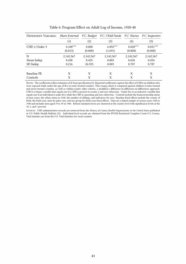
Table 6: Program E�ect on Adult Log of Income, 1920-40

Dependent Variable: Share External P.C. Budget P.C. Child Funds P.C. Nurses P.C. Inspectors

(1) (2) (3) (4) (5)

CHD x Under 5 0.100*** 0.000 6.892*** 0.028*** 0.031***(0.013) (0.000) (1.691) (0.008) (0.008)

N 2,142,567 2,142,567 2,142,567 2,142,567 2,142,567Mean Indep 0.438 8.425 0.003 0.636 0.454SD Indep 0.216 26.923 0.003 0.707 0.787

Baseline FE X X X X XControls X X X X XNotes: The coe�cients re�ect estimates ofβ from speci�cation (5). Reported coe�cients capture the e�ect of CHDs on children whowere exposed while under the age of �ve in early-treated counties. This young cohort is compared against children in later-treatedand never-treated counties, as well as within-county older cohorts, a modi�ed a di�erence-in-di�erence-in-di�erences approach.CHD is a binary variable that equals one if a CHD is present in county j and zero otherwise. Under �ve is an indicator variable thatequals one if an individual is under �ve while the CHD is operating and zero otherwise. Controls include the homeownership statusin base years, the urban status in 1940, the number of siblings, and indicators for race. Baseline �xed e�ects include the county ofbirth, the birth year, state-by-place size, and tax-group-by-birth-year �xed e�ects. Data are a linked sample of census years 1920 to1940 and includes men aged 19 to 39 in 1940. Robust standard errors are clustered at the county level with signi�cance levels at the10, 5, and 1 percent.Sources: CHD administrative records are retrieved from the History of County Health Organizations in the United States publishedin U.S. Public Health Bulletin 222. Individual-level records are obtained from the IPUMS Restricted Complete Count U.S. Census.Vital statistics are from the U.S. Vital Statistics for rural counties.

43

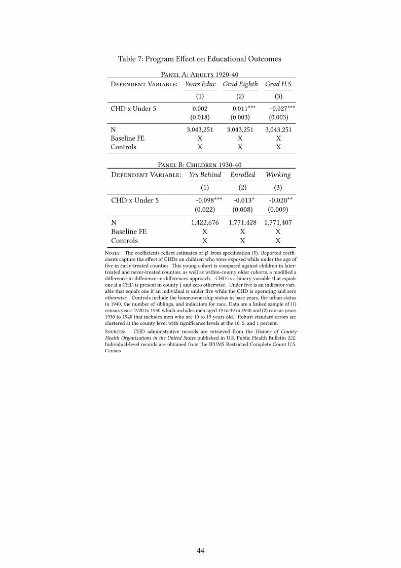
Table 7: Program E�ect on Educational Outcomes

Panel A: Adults 1920-40Dependent Variable: Years Educ Grad Eighth Grad H.S.

(1) (2) (3)

CHD x Under 5 0.002 0.011*** -0.027***(0.018) (0.003) (0.003)

N 3,043,251 3,043,251 3,043,251Baseline FE X X XControls X X X

Panel B: Children 1930-40Dependent Variable: Yrs Behind Enrolled Working

(1) (2) (3)

CHD x Under 5 -0.098*** -0.013* -0.020**(0.022) (0.008) (0.009)

N 1,422,676 1,771,428 1,771,407Baseline FE X X XControls X X X

Notes: The coe�cients re�ect estimates of β from speci�cation (5). Reported coe�-cients capture the e�ect of CHDs on children who were exposed while under the age of�ve in early-treated counties. This young cohort is compared against children in later-treated and never-treated counties, as well as within-county older cohorts, a modi�ed adi�erence-in-di�erence-in-di�erences approach. CHD is a binary variable that equalsone if a CHD is present in county j and zero otherwise. Under �ve is an indicator vari-able that equals one if an individual is under �ve while the CHD is operating and zerootherwise. Controls include the homeownership status in base years, the urban statusin 1940, the number of siblings, and indicators for race. Data are a linked sample of (1)census years 1920 to 1940 which includes men aged 19 to 39 in 1940 and (2) census years1930 to 1940 that includes men who are 10 to 19 years old. Robust standard errors areclustered at the county level with signi�cance levels at the 10, 5, and 1 percent.Sources: CHD administrative records are retrieved from the History of CountyHealth Organizations in the United States published in U.S. Public Health Bulletin 222.Individual-level records are obtained from the IPUMS Restricted Complete Count U.S.Census.

44

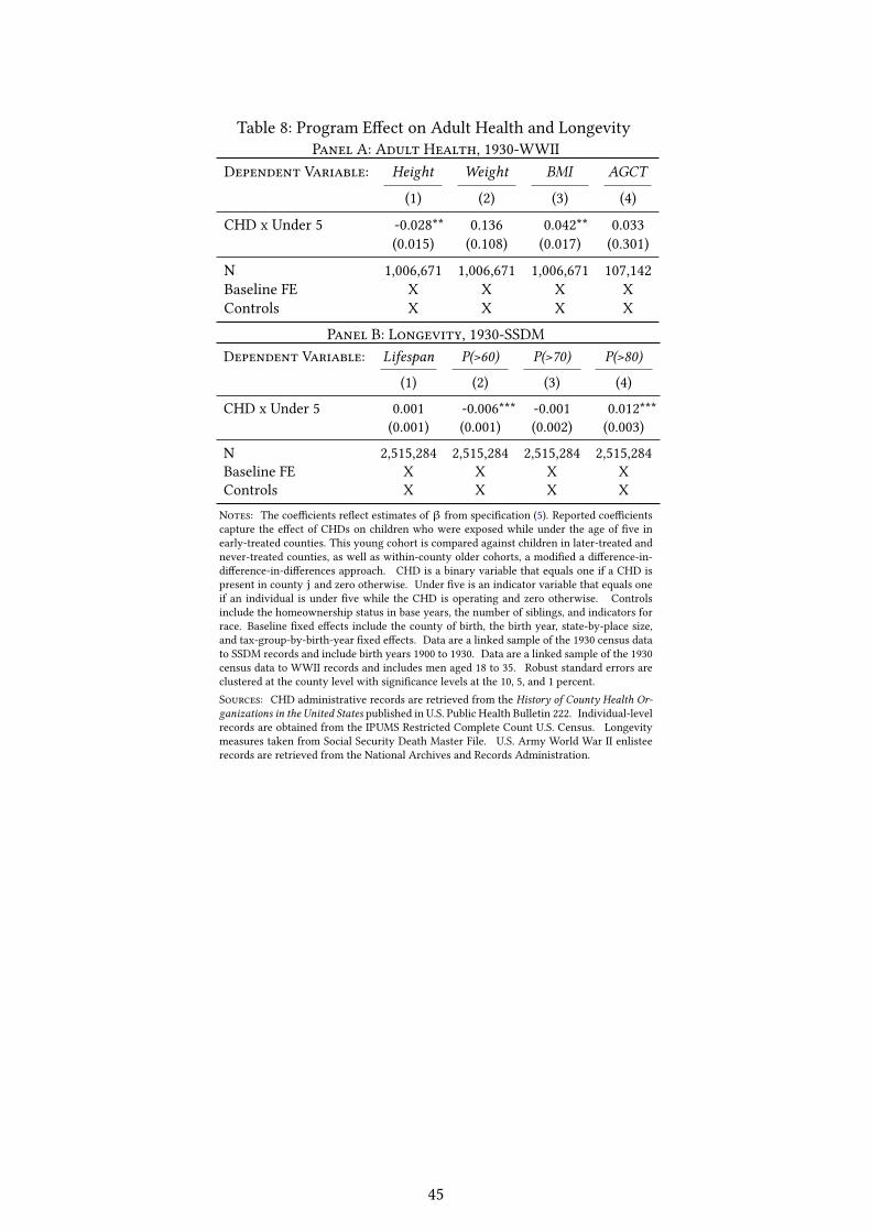
Table 8: Program E�ect on Adult Health and LongevityPanel A: Adult Health, 1930-WWII

Dependent Variable: Height Weight BMI AGCT

(1) (2) (3) (4)

CHD x Under 5 -0.028** 0.136 0.042** 0.033(0.015) (0.108) (0.017) (0.301)

N 1,006,671 1,006,671 1,006,671 107,142Baseline FE X X X XControls X X X X

Panel B: Longevity, 1930-SSDMDependent Variable: Lifespan P(>60) P(>70) P(>80)

(1) (2) (3) (4)

CHD x Under 5 0.001 -0.006*** -0.001 0.012***(0.001) (0.001) (0.002) (0.003)

N 2,515,284 2,515,284 2,515,284 2,515,284Baseline FE X X X XControls X X X XNotes: The coe�cients re�ect estimates of β from speci�cation (5). Reported coe�cientscapture the e�ect of CHDs on children who were exposed while under the age of �ve inearly-treated counties. This young cohort is compared against children in later-treated andnever-treated counties, as well as within-county older cohorts, a modi�ed a di�erence-in-di�erence-in-di�erences approach. CHD is a binary variable that equals one if a CHD ispresent in county j and zero otherwise. Under �ve is an indicator variable that equals oneif an individual is under �ve while the CHD is operating and zero otherwise. Controlsinclude the homeownership status in base years, the number of siblings, and indicators forrace. Baseline �xed e�ects include the county of birth, the birth year, state-by-place size,and tax-group-by-birth-year �xed e�ects. Data are a linked sample of the 1930 census datato SSDM records and include birth years 1900 to 1930. Data are a linked sample of the 1930census data to WWII records and includes men aged 18 to 35. Robust standard errors areclustered at the county level with signi�cance levels at the 10, 5, and 1 percent.Sources: CHD administrative records are retrieved from the History of County Health Or-ganizations in the United States published in U.S. Public Health Bulletin 222. Individual-levelrecords are obtained from the IPUMS Restricted Complete Count U.S. Census. Longevitymeasures taken from Social Security Death Master File. U.S. Army World War II enlisteerecords are retrieved from the National Archives and Records Administration.

45

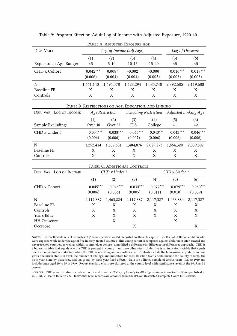
Table 9: Program E�ect on Adult Log of Income with Adjusted Exposure, 1920-40

Panel A: Adjusted Exposure AgeDep. Var.: Log of Income (adj Age) Log of Occscore

(1) (2) (3) (4) (5) (6)Exposure at Age Range: <5 5-10 10-15 15-20 <5 <5

CHD x Cohort 0.042*** 0.008* -0.002 -0.000 0.010*** 0.019***(0.006) (0.004) (0.004) (0.005) (0.003) (0.003)

N 1,661,140 1,695,378 1,428,294 1,085,748 2,892,685 2,119,688Baseline FE X X X X X XControls X X X X X X

Panel B: Restrictions on Age, Education, and LinkingDep. Var.: Log of Income Age Restriction Schooling Restriction Adjusted Linking Age

(1) (2) (3) (4) (5) (6)Sample Excluding: Over 30 Over 35 H.S. College >1 >2

CHD x Under 5 0.034*** 0.038*** 0.045*** 0.043*** 0.043*** 0.046***(0.006) (0.006) (0.007) (0.006) (0.006) (0.006)

N 1,252,414 1,657,631 1,404,876 2,029,273 1,864,320 2,039,807Baseline FE X X X X X XControls X X X X X X

Panel C: Additional ControlsDep. Var.: Log of Income CHD x Under 5 CHD x Under 1

(1) (2) (3) (4) (5) (6)

CHD x Cohort 0.045*** 0.046*** 0.034*** 0.077*** 0.079*** 0.060***(0.006) (0.006) (0.005) (0.011) (0.010) (0.009)

N 2,117,387 1,463,884 2,117,387 2,117,387 1,463,884 2,117,387Baseline FE X X X X X XControls X X X X X XYears Educ X X X X X XHH Occscore X XOccscore X X

Notes: The coe�cients re�ect estimates ofβ from speci�cation (5). Reported coe�cients capture the e�ect of CHDs on children whowere exposed while under the age of �ve in early-treated counties. This young cohort is compared against children in later-treated andnever-treated counties, as well as within-county older cohorts, a modi�ed a di�erence-in-di�erence-in-di�erences approach. CHD isa binary variable that equals one if a CHD is present in county j and zero otherwise. Under �ve is an indicator variable that equalsone if an individual is under �ve while the CHD is operating and zero otherwise. Controls include the homeownership status in baseyears, the urban status in 1940, the number of siblings, and indicators for race. Baseline �xed e�ects include the county of birth, thebirth year, state-by-place size, and tax-group-by-birth-year �xed e�ects. Data are a linked sample of census years 1920 to 1940 andincludes men aged 19 to 39 in 1940. Robust standard errors are clustered at the county level with signi�cance levels at the 10, 5, and 1percent.Sources: CHD administrative records are retrieved from the History of County Health Organizations in the United States published inU.S. Public Health Bulletin 222. Individual-level records are obtained from the IPUMS Restricted Complete Count U.S. Census.

46

References

Acemoglu, Daron and Simon Johnson, “Disease and development: the e�ect of life expectancy oneconomic growth,” Technical Report 6 2007.

Administration, Social Security et al., “Social Security Death Index, Master File. Social SecurityAdministration,” 2015.

A’Hearn, Brian, Jörg Baten, and Dorothee Crayen, “Quantifying Quantitative Literacy: Age Heap-ing and the History of Human Capital,” The Journal of Economic History, 2009, 69 (3), 783–808.

Aizer, Anna, Shari Eli, Joseph Ferrie, and Adriana Lleras-Muney, “The Long-Run Impact of CashTransfers to Poor Families,” The American Economic Review, 2016, 106 (4), 935–971.

Albanesi, Stefania and Claudia Olivetti, “Maternal health and the baby boom,” Quantitative Eco-nomics, 2014, 5 (2), 225–269.

and , “Gender Roles and Medical Progress,” Journal of Political Economy, 2016, 124 (3), 650–695.

Almond, Douglas, “Is the 1918 In�uenza Pandemic Over? Long-Term E�ects of In Utero In�uenzaExposure in the Post-1940 U.S. Population,” Journal of Political Economy, 2006, 114 (4), 672–712.

Alsan, Marcella and Claudia Goldin, “Watersheds in Infant Mortality: The Role of E�ective Waterand Sewerage Infrastructure, 1880 to 1915,” Technical Report, National Bureau of Economic Research2015.

Altenderfer, Marion E, “Full-Time Public Health Positions in Local Health Departments,” PublicHealth Reports (1896-1970), 1946, pp. 866–874.

Atack, Jeremy, Fred Bateman, andMary EschelbachGregson, ““Matchmaker, Matchmaker, MakeMe a Match” A General Personal Computer-Based Matching Program for Historical Research,” His-torical Methods: A Journal of Quantitative and Interdisciplinary History, 1992, 25 (2), 53–65.

Bailey, Martha, Connor Cole, Morgan Henderson, and Catherine Massey, “How Well Do Auto-mated Linking Methods Perform in Historical Samples? Evidence from New Ground Truth,” 2017.

Bailey, Martha J and Andrew Goodman-Bacon, “The War on Poverty’s Experiment in PublicMedicine: Community Health Centers and the Mortality of Older Americans,” The American Eco-nomic Review, 2015, 105 (3), 1067–1104.

Baird, Sarah, JoanHamoryHicks,Michael Kremer, andEdwardMiguel, “Worms at Work: Long-run Impacts of a Child Health Investment,” The Quarterly Journal of Economics, 2016, 131 (4), 1637–1680.

Beach, Brian, Joseph Ferrie, Martin Saavedra, and Werner Troesken, “Typhoid Fever, WaterQuality, and Human Capital Formation,” The Journal of Economic History, 2016, 76 (01), 41–75.

Behrman, Jere R, “Intrahousehold distribution and the family,” Handbook of Population and FamilyFconomics, 1997, 1, 125–187.

andMarkRRosenzweig, “Parental Allocations to Children: New Evidence on Bequest Di�erencesamong Siblings,” Review of Economics and Statistics, 2004, 86 (2), 637–640.

Ben-Porath, Yoram, “The Production of Human Capital and the Life Cycle of Earnings,” he Journalof Political Economy, 1967, pp. 352–365.

47

Bingham,Walter V, “Inequalities in Adult Capacity–From Military Data,” Science, 1946, 104, 147–152.

Bleakley, Hoyt, “Disease and Development: Evidence from Hookworm Eradication in the AmericanSouth,” The Quarterly Journal of Economics, 2007, 122 (1), 73.

, “Malaria Eradication in the Americas: A Retrospective Analysis of Childhood Exposure,” AmericanEconomic Journal: Applied economics, 2010, 2 (2).

Bozzoli, Carlos, Angus Deaton, and Climent Quintana-Domeque, “Adult Height and ChildhoodDisease,” Demography, 2009, 46 (4), 647–669.

Case, Anne and Christina Paxson, “Early Life Health and Cognitive Function in Old Age,” TheAmerican Economic Review, 2009, 99 (2), 104.

, Diana Lee, and Christina Paxson, “The Income Gradient in Children’s Health: A Comment onCurrie, Shields and Wheatley Price,” Journal of Health Economics, 2008, 27 (3), 801–807.

Center, Minnesota Population and Ancestry.com, IPUMS Restricted Complete Count Data, Univer-sity of Minnesota, 2017.

Chapin, Charles Value, Municipal Sanitation in the United States, Snow & Farnham, 1900.

, A Report on State Public Health Work: Based on a Survey of State Boards of Health, American MedicalAssn., 1916.

Clay, Karen, Je� Lingwall, and Melvin Stephens Jr, “Laws, Educational Outcomes, and Returnsto Schooling: Evidence from the Full Count 1940 Census,” Technical Report, National Bureau ofEconomic Research 2016.

Collins, William J and Robert AMargo, “Historical Perspectives on Racial Di�erences in Schoolingin the United States,” Handbook of the Economics of Education, 2006, 1, 107–154.

Currie, Janet, “Healthy, Wealthy, and Wise: Socioeconomic Status, Poor Health in Childhood, andHuman Capital Development,” Journal of Economic Literature, 2009, 47 (1), 87–122.

andDouglasAlmond, “Human capital development before age �ve,”Handbook of Labor Economics,2011, 4, 1315–1486.

Cutler, David and Grant Miller, “The role of public health improvements in health advances: Thetwentieth-century United States,” Demography, 2005, 42 (1), 1–22.

Davenport, Charles Benedict and Albert G Love, “Defects found in drafted men,” The Scienti�cMonthly, 1920, pp. 5–25.

Davis, Michael M., “How Healthy Are We?,” 1942.

Desmet, Klaus and Jordan Rappaport, “The Settlement of the United States, 1800 to 2000: The LongTransition Towards Gibrat’s Law,” Journal of Urban Economics, 2015.

Du�y, John, The Sanitarians: A History of American Public Health, University of Illinois Press, 1992.

Du�o, Esther, “Schooling and Labor Market Consequences of School Construction in Indonesia: Ev-idence from an Unusual Policy Experiment,” The American Economic Review, 2001, 91 (4), 795–813.

, Michael Greenstone, Raymond Guiteras, and Thomas Clasen, “Toilets can work: Short andmedium run health impacts of addressing complementarities and externalities in water and sanita-tion,” Technical Report, National Bureau of Economic Research 2015.

48

Engs, Ruth C, The Progressive Era’s Health Reform Movement: A Historical Dictionary, GreenwoodPublishing Group, 2003.

Feigenbaum, James J, “A Machine Learning Approach to Census Record Linking,” 2016.

and Christopher Muller, “Lead Exposure and Violent Crime in the Early Twentieth Century,”Explorations in Economic History, 2016, 62, 51–86.

Fernández, Raquel, Alessandra Fogli, and Claudia Olivetti, “Mothers and Sons: Preference For-mation and Female Labor Force Dynamics,” The Quarterly Journal of Economics, 2004, 119 (4), 1249–1299.

Ferrell, JohnA, Pauline AMead et al., “History of County Health Organizations in the United States1908-33.,” Public Health Bulletin, 1936, (222).

Ferrie, Joseph, “A new sample of Americans linked from the 1850 public use micro-sample of theFederal Census of Populations to the 1860 Federal Census Manuscripts,” Historical Methods, 1996,39, 141–156.

and Karen Rolf, “Socioeconomic status in childhood and health after age 70: A new longitudinalanalysis for the U.S., 1895–2005,” Explorations in Economic History, 2011, 48 (4), 445–460.

, , and Werner Troesken, “. . . Healthy, Wealthy, and Wise? Physical, Economic and CognitiveE�ects of Early Life Conditions on Later Life Outcomes in the US, 1915-2005,” in “Long-run Impactof Early Life Events II Workshop, National Poverty Center, University of Michigan” 2009.

Fishback, Price V, Michael R Haines, and Shawn Kantor, “The Impact of the New Deal on Blackand White Infant Mortality in the South,” Explorations in Economic History, 2001, 38 (1), 93–122.

, William C Horrace, and Shawn Kantor, “The impact of New Deal expenditures on mobilityduring the Great Depression,” Explorations in Economic History, 2006, 43 (2), 179–222.

Freeman, AllenWeir and Eugene Lindsay Bishop, A study of rural public health service, AmericanPublic Health Association, 1933.

Gerecke, Carlton, “US World War II Army Enlistment Records, 1938–1946,” National Archives andRecords Administration.

Grossman, Michael, “On the Concept of Health Capital and the Demand for Health,” Journal of Po-litical Economy, 1972, 80 (2), 223–255.

Grumstrup-Scott, Judith, Bernadette M Marriott et al., Body Composition and Physical Perfor-mance: Applications for the Military Services, National Academies Press, 1992.

Haines, Michael R, “The urban mortality transition in the United States, 1800-1940,” in “Annales dedémographie historique” number 1 Belin 2001, pp. 33–64.

, “Historical, Demographic, Economic, and Social Data: The United States, 1790-2002. ICPSR02896-v3,” Inter-university Consortium for Political and Social Research [distributor], 2010.

Headey, Derek, John Hoddinott, Disha Ali, Roman Tesfaye, and Mekdim Dereje, “The OtherAsian Enigma: Explaining the Rapid Reduction of Undernutrition in Bangladesh,” World Develop-ment, 2015, 66, 749–761.

HHS, “Health Resources and Services Administration, Maternal and Child Health Bureau. ChildHealth,” 2012.

49

Higgs, Robert, “Mortality in Rural America, 1870-1920: Estimates and Conjectures,” Explorations inEconomic History, 1973, 10 (2), 177–195.

Hoehn-Velasco, Lauren, “Explaining Declines in US Rural Mortality, 1910-1933: The Role of CountyHealth Departments,” Technical Report, Boston College Department of Economics 2016.

Hung, Peiyin, KatyKozhimannil, CarrieHenning-Smith, andMichelle Casey, “Closure of Hos-pital Obstetric Services Disproportionately A�ects Less-Populated Rural Counties,” 2017.

Jayachandran, Seema, Adriana Lleras-Muney, and Kimberly V Smith, “Modern medicine andthe twentieth century decline in mortality: evidence on the impact of sulfa drugs,” Technical Report 22010.

, , and , “Modern medicine and the twentieth century decline in mortality: evidence on theimpact of sulfa drugs,” American Economic Journal: Applied Economics, 2010, 2 (2), 118–146.

and , “Life Expectancy and Human Capital Investments: Evidence from Maternal Mortality De-clines,” Technical Report 1 2009.

Kitchens, Carl, “A Dam Problem: TVA’s Fight Against Malaria, 1926–1951,” The Journal of EconomicHistory, 2013, 73 (03), 694–724.

Lancaster, Lane, Government in Rural America, JSTOR, 1937.

Long, Jason and Joseph Ferrie, “Intergenerational Occupational Mobility in Great Britain and theUnited States since 1850,” The American Economic Review, 2013, 103 (4), 1109–1137.

Lumsden, Leslie Leon, “Cooperative Rural Health Work of the Public Health Service,” Public HealthReports (1896-1970), 1920-30.

Maluccio, John A, John Hoddinott, Jere R Behrman, Reynaldo Martorell, Agnes R Quisumb-ing, andAryehD Stein, “The Impact of Improving Nutrition During Early Childhood on Educationamong Guatemalan Adults,” The Economic Journal, 2009, 119 (537), 734–763.

Margo, Robert A, “Educational Achievement In Segregated School Systems: The E�ects of "Separate-but-Equal",” The American Economic Review, 1986, 76 (4), 794–801.

, “Race, Educational Attainment, and the 1940 Census,” The Journal of Economic History, 1986, 46 (1),189–198.

, Race and Schooling in the South, 1880-1950, University of Chicago Press, 1990.

Maron, Dina Fine, “Maternal Health Care Is Disappearing in Rural America,” Scienti�c American,2017.

Miguel, Edward andMichael Kremer, “Worms: Identifying Impacts on Education and Health in thePresence of Treatment Externalities,” Econometrica, 2004, pp. 159–217.

Moehling, Carolyn M and Melissa A Thomasson, “Saving Babies: The Impact of Public EducationPrograms on Infant Mortality,” Demography, 2014, 51 (2), 367–386.

of the Census United States Department of Commerce, Bureau, Wealth, Public Debt, and Taxa-tion: 1922, US Government Printing O�ce, 1924.

of the Census United States Vital Statistics, Bureau, Mortality Statistics: Vital Statistics of theUnited States: 1890-1938, United States Bureau of the Census, 1890-1938.

50

Olivetti, Claudia and M Daniele Paserman, “In the Name of the Son (and the Daughter): Intergen-erational Mobility in the United States, 1850–1940,” The American Economic Review, 2015, 105 (8),2695–2724.

Oster, Emily, Ira Shoulson, and E Dorsey, “Limited Life Expectancy, Human Capital and HealthInvestments,” The American Economic Review, 2013, 103 (5), 1977–2002.

Probst, Janice C, Sarah B Laditka, Jong-Yi Wang, and Andrew O Johnson, “E�ects of residenceand race on burden of travel for care: cross sectional analysis of the 2001 US National HouseholdTravel Survey,” BMC Health Services Research, 2007, 7 (1), 40.

Rappaport, Jordan, “Moving to nice weather,” Regional Science and Urban Economics, 2007, 37 (3),375–398.

Ravenel, Mazÿck Porcher, A half century of public health: jubilee historical volume of the AmericanPublic Health Association, in commemoration of the �ftieth anniversary celebration of its foundation,New York City, November 14-18, 1921, New York: American Public Health Association, 1921.

Rosen, George, A History of Public Health, JHU Press, 2015.

Stiles, CHWardell, “The Rural Health Movement,” The ANNALS of the American Academy of Politicaland Social Science, 1911, 37 (2), 123–126.

Taft, Robert L, Name Search Techniques number 1, Bureau of Systems Development, New York StateIdenti�cation and Intelligence System, 1970.

Troesken, Werner, “Typhoid Rates and the Public Acquisition of Private Waterworks, 1880–1920,”The Journal of Economic History, 1999, 59 (04), 927–948.

, “Race, Disease, and the Provision of Water in American Cities, 1889–1921,” The Journal of EconomicHistory, 2001, 61 (03), 750–776.

and Rick Geddes, “Municipalizing American Waterworks, 1897–1915,” Journal of Law, Economics,and Organization, 2003, 19 (2), 373–400.

Wallis, John Joseph, “A History of the Property Tax in America,” Property taxation and local govern-ment �nance, 2001, pp. 123–47.

Winkler, William E, “The State of Record Linkage and Current Research Problems,” in “StatisticalResearch Division, US Census Bureau” Citeseer 1999.

Wood, Thomas Denison, Health Essentials for Rural School Children, Press of American Medical As-sociation, 1921.

Zivin, Joshua Gra� and Matthew Neidell, “Environment, Health, and Human Capital,” Journal ofEconomic Literature, 2013, 51 (3), 689–730.

51

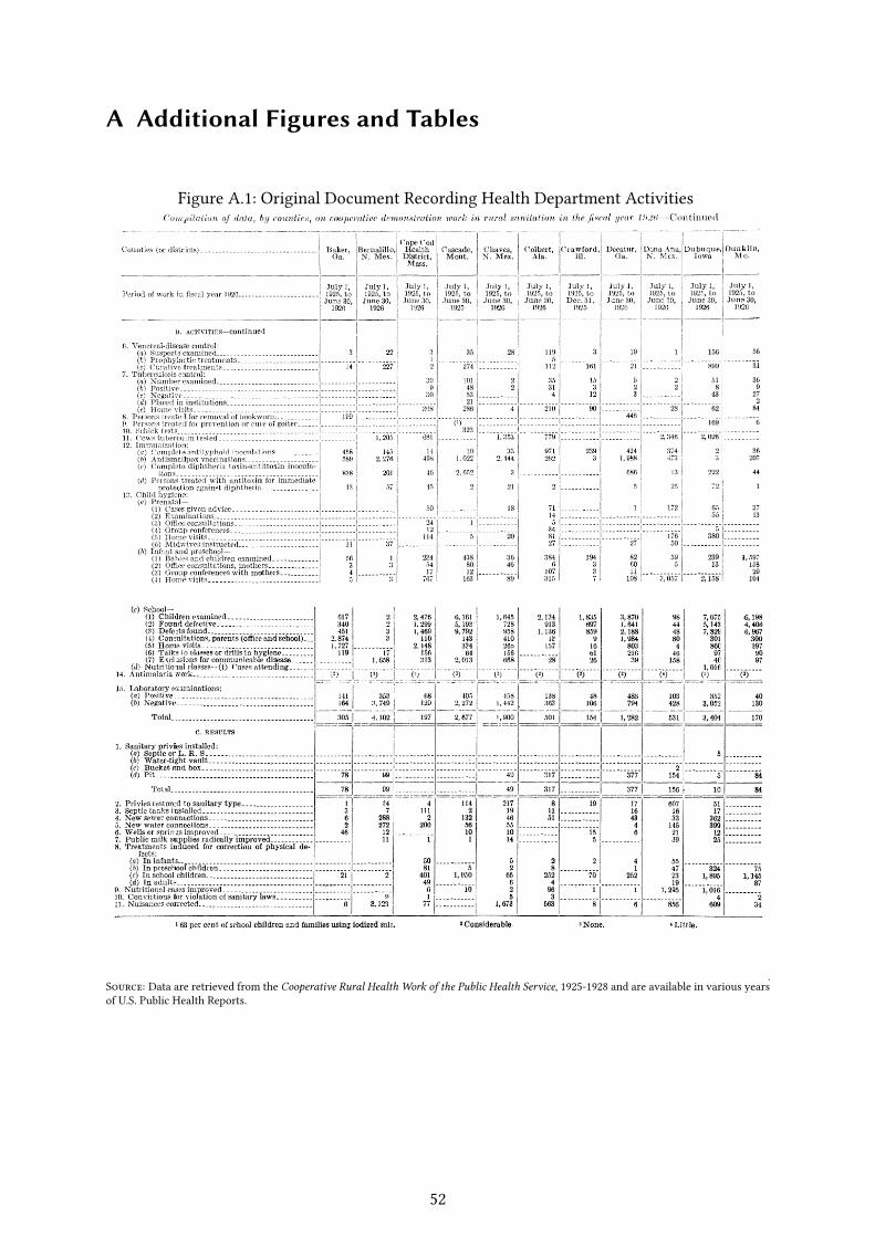
A Additional Figures and Tables

Figure A.1: Original Document Recording Health Department Activities

Source: Data are retrieved from the Cooperative Rural Health Work of the Public Health Service, 1925-1928 and are available in various yearsof U.S. Public Health Reports.

52

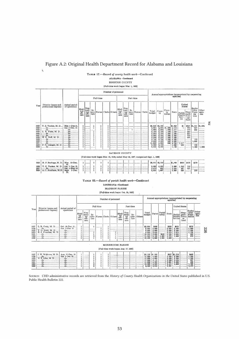
Figure A.2: Original Health Department Record for Alabama and Louisiana

Source: CHD administrative records are retrieved from the History of County Health Organizations in the United States published in U.S.Public Health Bulletin 222.

53

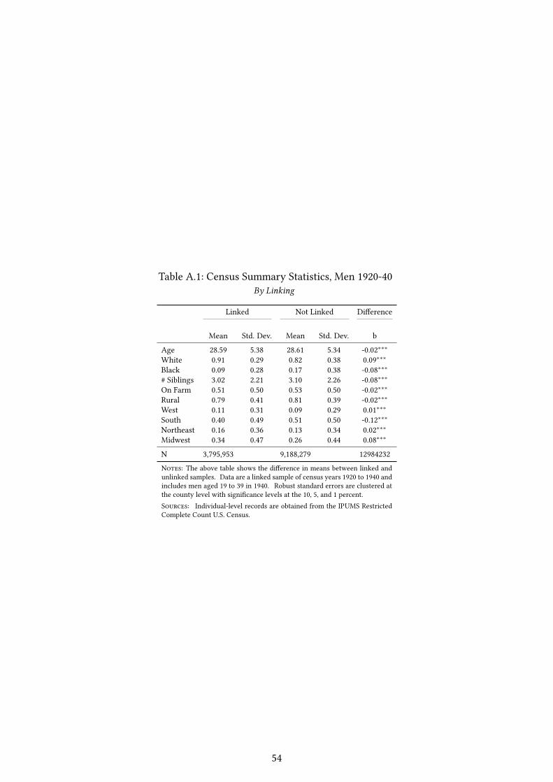
Table A.1: Census Summary Statistics, Men 1920-40By Linking

Linked Not Linked Di�erence

Mean Std. Dev. Mean Std. Dev. b

Age 28.59 5.38 28.61 5.34 -0.02∗∗∗White 0.91 0.29 0.82 0.38 0.09∗∗∗Black 0.09 0.28 0.17 0.38 -0.08∗∗∗# Siblings 3.02 2.21 3.10 2.26 -0.08∗∗∗On Farm 0.51 0.50 0.53 0.50 -0.02∗∗∗Rural 0.79 0.41 0.81 0.39 -0.02∗∗∗West 0.11 0.31 0.09 0.29 0.01∗∗∗South 0.40 0.49 0.51 0.50 -0.12∗∗∗Northeast 0.16 0.36 0.13 0.34 0.02∗∗∗Midwest 0.34 0.47 0.26 0.44 0.08∗∗∗

N 3,795,953 9,188,279 12984232

Notes: The above table shows the di�erence in means between linked andunlinked samples. Data are a linked sample of census years 1920 to 1940 andincludes men aged 19 to 39 in 1940. Robust standard errors are clustered atthe county level with signi�cance levels at the 10, 5, and 1 percent.Sources: Individual-level records are obtained from the IPUMS RestrictedComplete Count U.S. Census.

54

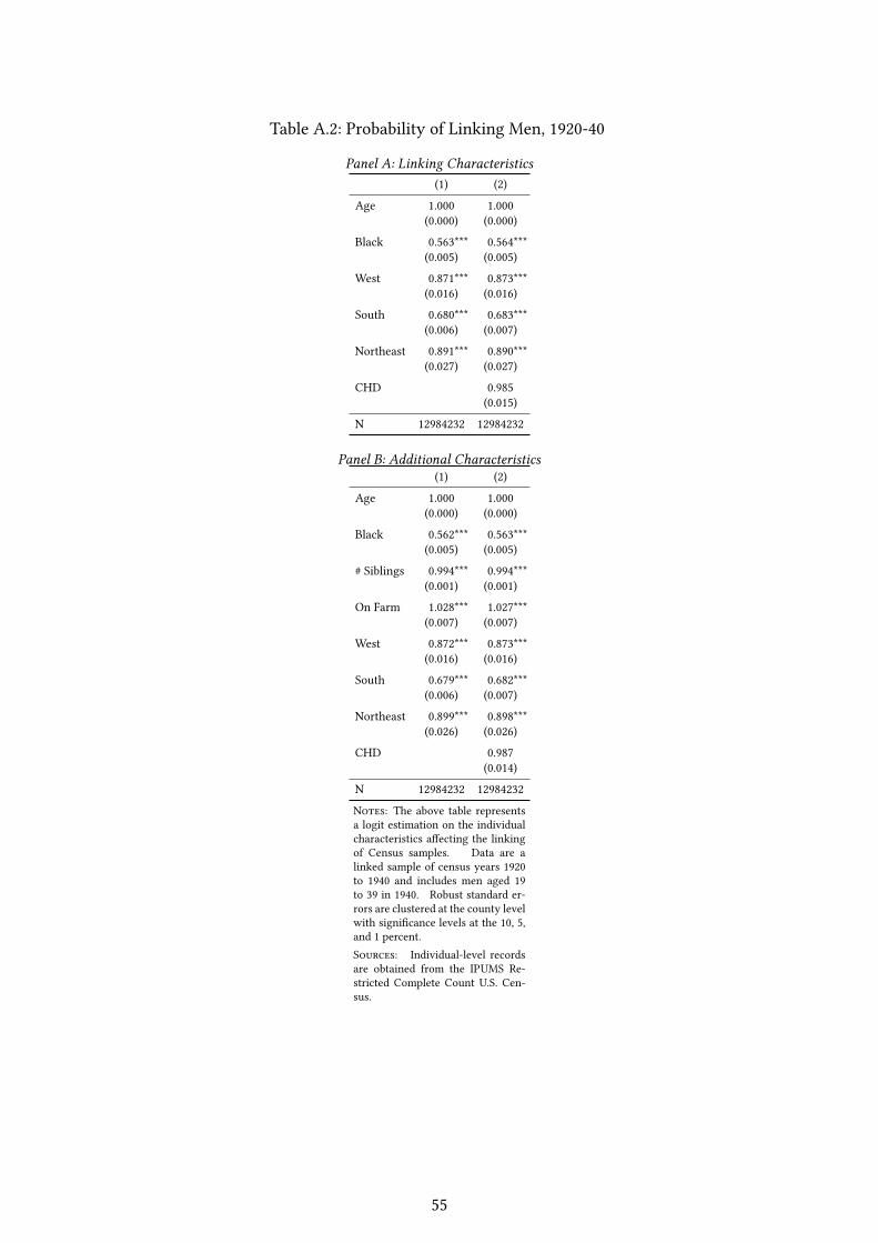
Table A.2: Probability of Linking Men, 1920-40

Panel A: Linking Characteristics(1) (2)

Age 1.000 1.000(0.000) (0.000)

Black 0.563*** 0.564***(0.005) (0.005)

West 0.871*** 0.873***(0.016) (0.016)

South 0.680*** 0.683***(0.006) (0.007)

Northeast 0.891*** 0.890***(0.027) (0.027)

CHD 0.985(0.015)

N 12984232 12984232

Panel B: Additional Characteristics(1) (2)

Age 1.000 1.000(0.000) (0.000)

Black 0.562*** 0.563***(0.005) (0.005)

# Siblings 0.994*** 0.994***(0.001) (0.001)

On Farm 1.028*** 1.027***(0.007) (0.007)

West 0.872*** 0.873***(0.016) (0.016)

South 0.679*** 0.682***(0.006) (0.007)

Northeast 0.899*** 0.898***(0.026) (0.026)

CHD 0.987(0.014)

N 12984232 12984232

Notes: The above table representsa logit estimation on the individualcharacteristics a�ecting the linkingof Census samples. Data are alinked sample of census years 1920to 1940 and includes men aged 19to 39 in 1940. Robust standard er-rors are clustered at the county levelwith signi�cance levels at the 10, 5,and 1 percent.Sources: Individual-level recordsare obtained from the IPUMS Re-stricted Complete Count U.S. Cen-sus.

55

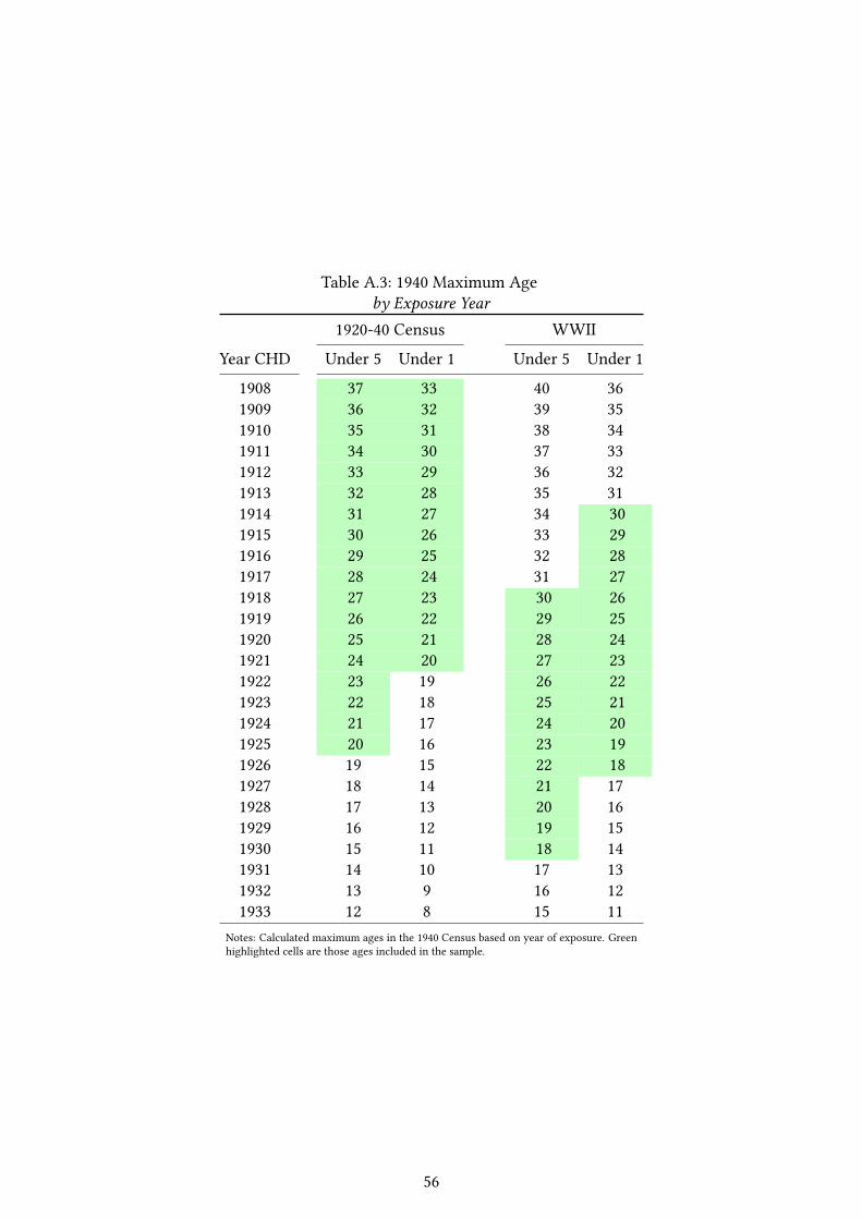
Table A.3: 1940 Maximum Ageby Exposure Year

1920-40 Census WWII

Year CHD Under 5 Under 1 Under 5 Under 1

1908 37 33 40 361909 36 32 39 351910 35 31 38 341911 34 30 37 331912 33 29 36 321913 32 28 35 311914 31 27 34 301915 30 26 33 291916 29 25 32 281917 28 24 31 271918 27 23 30 261919 26 22 29 251920 25 21 28 241921 24 20 27 231922 23 19 26 221923 22 18 25 211924 21 17 24 201925 20 16 23 191926 19 15 22 181927 18 14 21 171928 17 13 20 161929 16 12 19 151930 15 11 18 141931 14 10 17 131932 13 9 16 121933 12 8 15 11

Notes: Calculated maximum ages in the 1940 Census based on year of exposure. Greenhighlighted cells are those ages included in the sample.

56

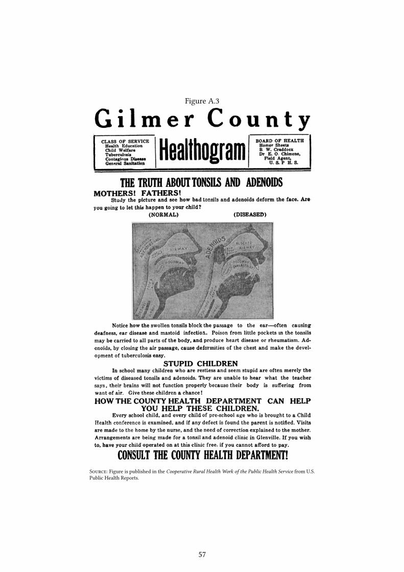
Figure A.3

Source: Figure is published in the Cooperative Rural Health Work of the Public Health Service from U.S.Public Health Reports.

57

B State-level CHD Adoption

States that operated CHDs were principally in the West and South, with exceptions in selectMidwestern states. Initially, the lopsided distribution throughout the nation appears related to thehealth conditions in the adopting states. On a more careful survey of the background literature, theadoption throughout these regions seems to be based on the structure of local government. In NewEngland and the majority of the Midwestern states, the town or township is the main political unit, andthese towns are the principal providers of local public goods, which include sanitary administration(Chapin (1900)).43 In New England there are only a few uninhabited areas that are not governed by atown. Throughout the New England states, the towns are contiguous, and a person cannot leave onetown without crossing into the jurisdiction of another.

In the South and West, on the other hand, "the county board of health has...been establishedto look after the sanitary interests of the people outside of the incorporated municipalities" (Chapin(1900)). This di�erence in the organization of local government, appears to be the primary force a�ect-ing the adoption of the county-level movement in health.44 In states that are the exception to the rule,including Ohio and Michigan, legislation was passed that required the organization of county-levelservices. This legislation was intended to create more e�cient organizations that could operate withenough scale to be e�ective against illness.45

While it is true that townships in the North set up town-level services, these services were oftenine�ective due to the weak �nances of the small populations. Rather than being subpar to the townlevel, it was "generally agreed that the county is the smallest feasible unit from the standpoint ofe�ciency of service and administration. In most sections, the use of the county makes it possible toabandon the large number of ine�ective organizations found in villages and townships" (?). To testwhether the strength of local government di�ers across treated and untreated states, I compare thetaxation power of state and local governments. Taxation is the clearest measure of the in�uence ofgovernment and captures both the wealth and revenue at each level.

Table ?? shows the mean value of the per capita taxes and property values across CHD and non-

43The regional di�erences in the political divisions was not a new occurrence, and evolved, beginning with thelocal government in the colonial era (Chapin (1900) pp. 6).

44These states include the New England states, Illinois, Iowa, Michigan, Minnesota, New Jersey, New York, Ohio,Pennsylvania, and Wisconsin.

45"The Michigan township was made a health authority in 1846 when, as one investigator put it, ‘diseases werethought to arise from smells and cemeteries, and when anyone able to detect an odor or manage a cemeterycould have quali�ed as a health o�cer." Such tiny areas, many of them too poor to perform their otherfunctions without state assistance, are unable to a�ord the personnel or the equipment needed to carry outa health program of any sort—and a health program is commonly regarded as of much less importance than,for example, education or roads. The health o�cers employed are more often than not untrained, serve intheir spare time, are paid only nominal salaries, and are quite unconvinced of the value of the scienti�c healthmeasures recommended by the state department which exercises a nominal supervision over them. Of the1,160 township health o�cers in Michigan, 660 are not physicians, while in Indiana townships many of themare paid as little as ten dollars a year. The post is a minor avocation of its holder and the work consists inmost places of "an occasional quarantine, an abatement of a nuisance, and a lighting of fumigators followingquarantine" pp. 336 ?

58

CHD states. In treated states, municipal taxes are lower per capita. Even more convincing, the share ofthe tax burden from municipal governments is lower, while the county level is higher. This di�erencein the share of taxes reveals the relative di�erences in the power structure across adopting and non-adopting states. County governments are relatively stronger in areas that adopted, while municipalgovernments are stronger in states that did not. No di�erence appears across property values or statetaxes. The comparison of means across CHD and non-CHD states reveals that as measured by taxationpower, municipal governments are weaker in adopting states. Adopting states, however, are no lesswealthy and have similar tax revenue at the state level of governance.

A second check on the adoption tests whether CHD states have di�erent, or even better, stateboards of health. It is possible that adopting states may have had a higher propensity toward healththan non-adopting states. To test this, the pre-adoption strength of the state boards of health is takenfrom Chapin (1916), which reports the quality and expenditures of each state. Here across adoption, thequality of the state board, the per capita prior expenditures on health and the measure of how the stateboard is elected appears no di�erent. Treatment is not selected based on the structure or expenditureof the state board of health.

59

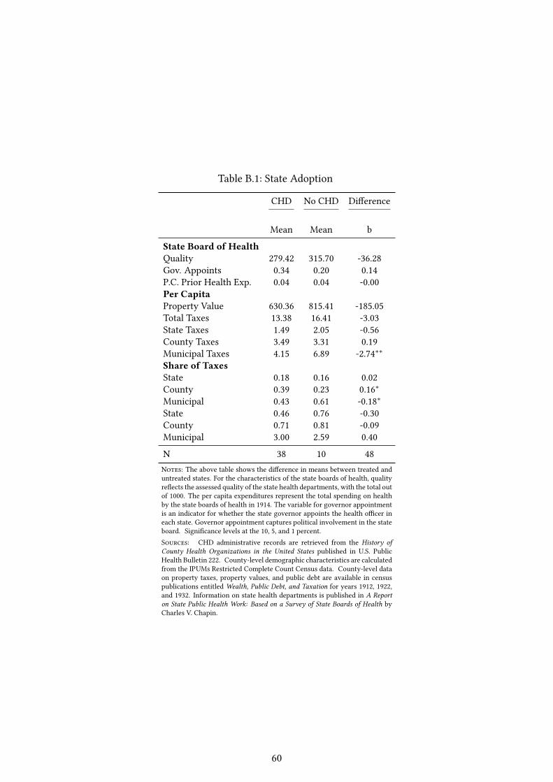
Table B.1: State Adoption

CHD No CHD Di�erence

Mean Mean b

State Board of HealthQuality 279.42 315.70 -36.28Gov. Appoints 0.34 0.20 0.14P.C. Prior Health Exp. 0.04 0.04 -0.00Per CapitaProperty Value 630.36 815.41 -185.05Total Taxes 13.38 16.41 -3.03State Taxes 1.49 2.05 -0.56County Taxes 3.49 3.31 0.19Municipal Taxes 4.15 6.89 -2.74∗∗Share of TaxesState 0.18 0.16 0.02County 0.39 0.23 0.16∗Municipal 0.43 0.61 -0.18∗State 0.46 0.76 -0.30County 0.71 0.81 -0.09Municipal 3.00 2.59 0.40

N 38 10 48Notes: The above table shows the di�erence in means between treated anduntreated states. For the characteristics of the state boards of health, qualityre�ects the assessed quality of the state health departments, with the total outof 1000. The per capita expenditures represent the total spending on healthby the state boards of health in 1914. The variable for governor appointmentis an indicator for whether the state governor appoints the health o�cer ineach state. Governor appointment captures political involvement in the stateboard. Signi�cance levels at the 10, 5, and 1 percent.Sources: CHD administrative records are retrieved from the History ofCounty Health Organizations in the United States published in U.S. PublicHealth Bulletin 222. County-level demographic characteristics are calculatedfrom the IPUMs Restricted Complete Count Census data. County-level dataon property taxes, property values, and public debt are available in censuspublications entitled Wealth, Public Debt, and Taxation for years 1912, 1922,and 1932. Information on state health departments is published in A Reporton State Public Health Work: Based on a Survey of State Boards of Health byCharles V. Chapin.

60

C CHD Health E�ects

C.1 Mortality

I exploit variation in the timing and the location of CHDs to capture the e�ect of health depart-ment entry on mortality. More speci�cally, I track mortality before and after CHD entry using a �exibleevent study. I follow a similar design to Bailey and Goodman-Bacon (2015), where the authors used anevent-study to track the rollout of Community Health Centers. This event-study speci�cation accountsfor the pattern of mortality surrounding CHD entry and follows mortality changes in each year beforeand after entry. Most importantly, tracking mortality in the period leading up to CHD entry directstests for spikes in mortality prior to health department arrival. Mortality changes before and afterentry are compared to the year before CHD arrival as well as conditions in never-treated counties.

To test how CHD access a�ects the evolution of county-level mortality, I estimate the followingequation:

Mjst = aj + ηst + πhjt +

14∑m=−3

βmCHDjm + X ′jtγ+ εjst (7)

where Mjst is the mortality rate in county j and time t = 1910, ..., 1936. County �xed e�ects, aj,control for factors would a�ect selection into treatment by absorbing time-invariant characteristicsof counties. ηst captures state-by-year �xed e�ects, such as state-level adoption of Sheppard-Townerfunding, higher state participation in the CHD program, or epidemic conditions within the state. πhjtare the tax-group-by-year �xed e�ects, which controls for the evolution of local government size.46

εjst is the regression error. Xjt are county-level controls. Controls include the homeownershipstatus in base years, the urban status in 1940, the number of siblings, and indicators for race.

CHD activity is captured by the event-study indicator variable, CHDjm. CHDjm represents theentry of a health department into county j at periodm = 0. m represents the period relative to entryat period zero. m ranges from three years prior to CHD entry to 14 years after CHD entry.47 The yearbefore CHD implementation,m = −1, is the excluded and provides a baseline for mortality before andafter implementation. The excluded period includes both treated counties in the year before the CHDopened as well as never-treated counties. The event-study speci�cation directly checks the assumptionthat pre-treatment changes in mortality conditions are uncorrelated with CHD timing and placement inthe periods just before treatment,m = −3, andm = −2. The main e�ect is captured in post-treatmentdummy variables,m = 1, 2, ...14, which is relative to the pre-treatment period,m = −1.

46Each group dummy variable represents the percentile ranking of taxation relative to other counties. Thegroups include percentiles from 0-20, 20-40, 40-60, 60-80, 80-100. These dummy variables are then interactedwith year dummy variables

47More formally, m indicates each observation’s timing relative to opening a CHD in county j in period zero.m is the di�erence between time t and the year the CHD opened, T , wherem = t− T .

61

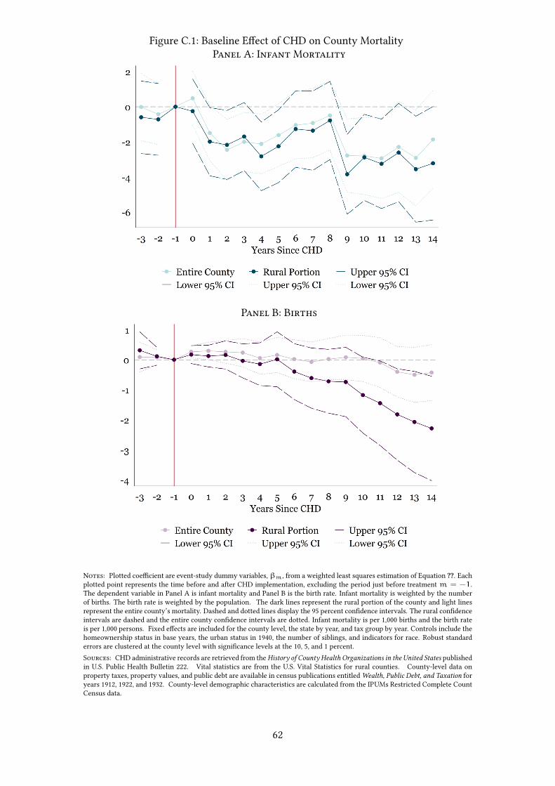
Figure C.1: Baseline E�ect of CHD on County MortalityPanel A: Infant Mortality

Panel B: Births

Notes: Plotted coe�cient are event-study dummy variables,βm, from a weighted least squares estimation of Equation ??. Eachplotted point represents the time before and after CHD implementation, excluding the period just before treatment m = −1.The dependent variable in Panel A is infant mortality and Panel B is the birth rate. Infant mortality is weighted by the numberof births. The birth rate is weighted by the population. The dark lines represent the rural portion of the county and light linesrepresent the entire county’s mortality. Dashed and dotted lines display the 95 percent con�dence intervals. The rural con�denceintervals are dashed and the entire county con�dence intervals are dotted. Infant mortality is per 1,000 births and the birth rateis per 1,000 persons. Fixed e�ects are included for the county level, the state by year, and tax group by year. Controls include thehomeownership status in base years, the urban status in 1940, the number of siblings, and indicators for race. Robust standarderrors are clustered at the county level with signi�cance levels at the 10, 5, and 1 percent.Sources: CHD administrative records are retrieved from the History of County Health Organizations in the United States publishedin U.S. Public Health Bulletin 222. Vital statistics are from the U.S. Vital Statistics for rural counties. County-level data onproperty taxes, property values, and public debt are available in census publications entitled Wealth, Public Debt, and Taxation foryears 1912, 1922, and 1932. County-level demographic characteristics are calculated from the IPUMs Restricted Complete CountCensus data.

62

Figure ?? plots the coe�cients from the event-study dummy variables speci�ed in Equation ??.Panel A shows the infant mortality rate in blue and Panel B shows the birth rate. Each plotted linerepresents a weighted least squares estimation of the county-level mortality rate, with the birth rateweighted by the population and the infant mortality weighted by the number of births. The plottedpoints connected by solid lines represent the estimated coe�cients on the county-level mortality rate.The dark lines represent the rural portion of the county and light lines represent the entire county’smortality. Dashed and dotted lines display the 95 percent con�dence intervals. The rural con�denceintervals are dashed and the entire county con�dence intervals are dotted.

Focusing on infant mortality in Panel A, the plotted point estimates portray a de�nite responseto the CHD. One period after the health department opens, infant mortality declines by two deaths per1,000 births. This lower infant mortality persists through period six with the point estimates hoveringaround a two death reduction in infant mortality. Then in periods six through eight, the CHD e�ectdiminishes, and while infant mortality is still lower than the pre-treatment level, the con�dence inter-vals include zero. In period nine the top con�dence interval drops and remains under zero through theremainder of the study. The e�ect on infant mortality appears stark when comparing to pre-treatmentlevels of infant mortality. In rural areas, there is little evidence of a spike in mortality just before entry.For the full county, there is a rise in mortality in period zero, but this e�ect is not statistically di�erentfrom zero.

As CHDs reduced infant mortality in treated counties, the availability of health services could alsoimpact the county-level birth rate. To test whether this is the case, Panel B of Figure ?? plots the pointestimates for the event study on the birth rate with the coe�cients weighted by the county population.For both the full county and the rural portion of the county, the birth rate appears to slightly increasefor two to three periods after the health department arrives, but the e�ect is not statistically signi�cant.Overall, there is little perceptible e�ect on the birth rate.

C.2 State-specific By-Cause Mortality and Morbidity

I test correlations of CHD entry with varying measures of health using a simple di�erence-in-di�erence framework.48 I do not attempt to establish causality as the availability of data is quite limited.To estimate the di�erence in mortality after the arrival of a health department, I test the followingequation:

mjt = α+ β(CHDj × Postt) + λPostt + aj + εjt (8)

48The data used in this section on based the archival work of Carl Kitchens, and generously shared for thepurposes of this paper. To attain morbidity records, I digitized the state public health reports collected for ?.

63

where is the mjt county-level mortality (or morbidity) in year t. CHDj indicates treatment with aCHD and Postt indicates the post period. aj is a county �xed e�ect. εjt is the regression error. Forthe available data, the equation captures the change in mortality for CHD counties after the CHDarrives.

Morbidity

A select number of states separately report the number of instances of each major illness by cause.I use this data to examine which diseases CHDs were most e�ective at reducing. I test Equation ?? overthe number of reported illnesses from state-level health reports in Alabama and Michigan. For thesestates, I create two groups of illnesses, those which a CHD could administer preventative or curativemeasure and unpreventable diseases. CHDs could mainly target typhoid, diphtheria, and smallpox.After 1923 all three illnesses had vaccinations available, and diphtheria antitoxin existed earlier in theperiod. I expect that CHDs will reduce the preventable illnesses, but as a placebo test, CHDs should beine�ective at reducing other types of disease.

Table ?? Panel A shows the results. For illnesses that the CHD could vaccinate against, the healthdepartment reduced instances of illnesses by 10 cases in Alabama and four in Michigan. By contrast,CHDs were ine�ective against non-vaccine illnesses, including TB. The decline in preventable diseasesreveals that CHDs were e�ective at reducing the diseases which they could administer treatment orprevention against. The most plausible explanation for this e�ect is either a water puri�cation storyor a vaccination story. Based on the e�ectiveness of CHDs through exams of infants, it is likely thecase that CHDs administered prevention through vaccination.

To check whether CHDs operated purely through water puri�cation, I report typhoid separatelyfor both states. In Michigan, the CHD had no signi�cant e�ect on typhoid mortality. For Alabama, thereis a reduction in typhoid but is only half of the e�ect of vaccine-preventable illnesses. The impact ofCHDs does not appear to be fully explained by improvements in water and drainage. The impact of theCHD is also seen in diphtheria and smallpox which suggests that while there were bene�cial sanitatione�orts, the health departments also promoted prevention and treatment of disease.

Overall, CHDs counties show reductions in illnesses that were preventable by the CHD. Theseillnesses include diphtheria, smallpox, and typhoid. A portion of e�ectiveness could be explained bybetter vaccination from the health department, but the declines in typhoid alone suggest that CHDcounties may have also improved water and drainage or reduced exposure to water-borne disease.

Maternal Mortality

Due to the declines in infant mortality, there might also be an e�ect on maternal deaths thatare not perceptible in overall mortality. To measure the impact of the CHD on maternal mortality,select states provide data during the period studied. I test maternal mortality in North Carolina and

64

Michigan to investigate whether CHDs improved the birth conditions in treated counties. Table ??

Panel B presents the results. CHD exposure reduced maternal mortality by two deaths per 1,000 births.This diminished maternal mortality is similar to the improvement in infant mortality and suggests thatCHDs were e�ective at improving the health of women and children surrounding pregnancy and birth.

65

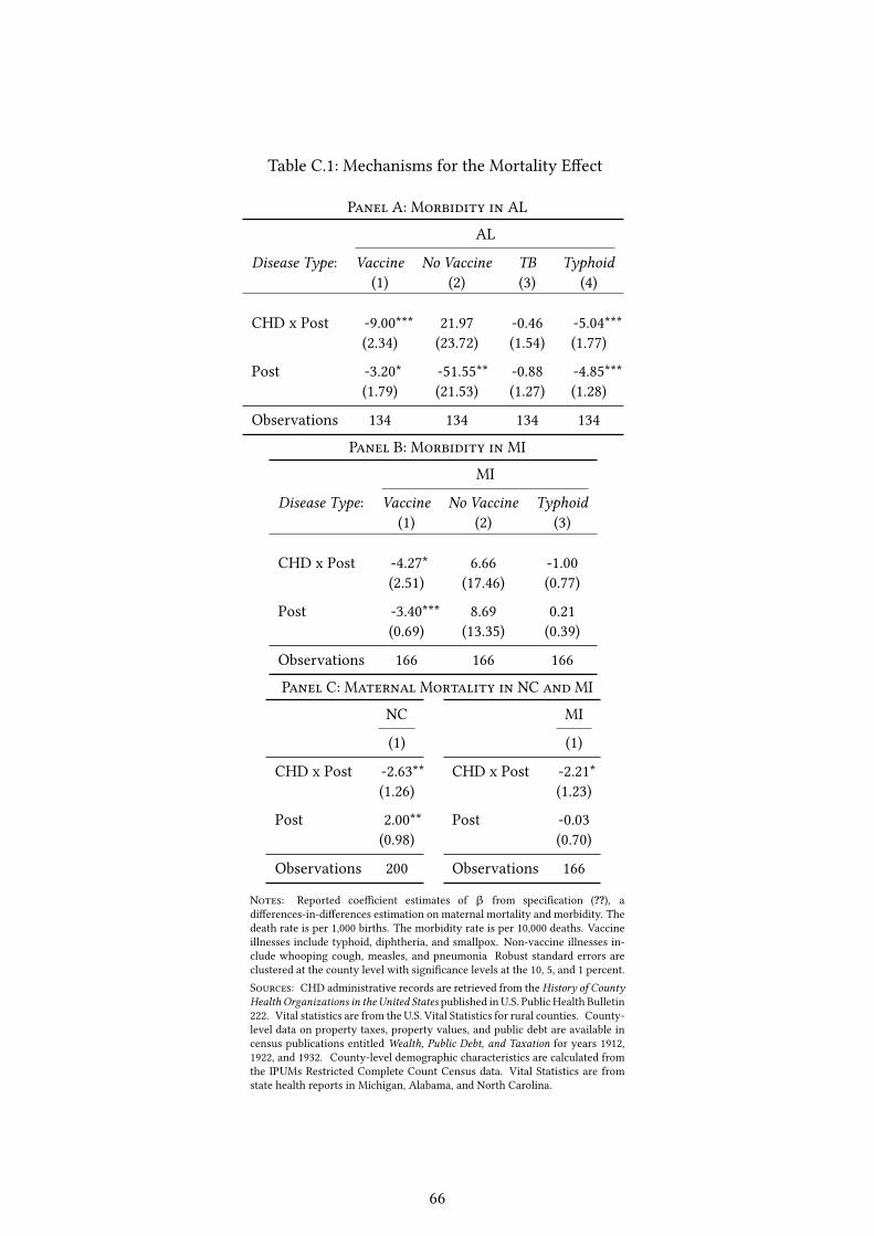
Table C.1: Mechanisms for the Mortality E�ect

Panel A: Morbidity in AL

AL

Disease Type: Vaccine No Vaccine TB Typhoid(1) (2) (3) (4)

CHD x Post -9.00*** 21.97 -0.46 -5.04***(2.34) (23.72) (1.54) (1.77)

Post -3.20* -51.55** -0.88 -4.85***(1.79) (21.53) (1.27) (1.28)

Observations 134 134 134 134

Panel B: Morbidity in MI

MI

Disease Type: Vaccine No Vaccine Typhoid(1) (2) (3)

CHD x Post -4.27* 6.66 -1.00(2.51) (17.46) (0.77)

Post -3.40*** 8.69 0.21(0.69) (13.35) (0.39)

Observations 166 166 166

Panel C: Maternal Mortality in NC and MI

NC

(1)

CHD x Post -2.63**(1.26)

Post 2.00**(0.98)

Observations 200

MI

(1)

CHD x Post -2.21*(1.23)

Post -0.03(0.70)

Observations 166

Notes: Reported coe�cient estimates of β from speci�cation (??), adi�erences-in-di�erences estimation on maternal mortality and morbidity. Thedeath rate is per 1,000 births. The morbidity rate is per 10,000 deaths. Vaccineillnesses include typhoid, diphtheria, and smallpox. Non-vaccine illnesses in-clude whooping cough, measles, and pneumonia Robust standard errors areclustered at the county level with signi�cance levels at the 10, 5, and 1 percent.Sources: CHD administrative records are retrieved from the History of CountyHealth Organizations in the United States published in U.S. Public Health Bulletin222. Vital statistics are from the U.S. Vital Statistics for rural counties. County-level data on property taxes, property values, and public debt are available incensus publications entitled Wealth, Public Debt, and Taxation for years 1912,1922, and 1932. County-level demographic characteristics are calculated fromthe IPUMs Restricted Complete Count Census data. Vital Statistics are fromstate health reports in Michigan, Alabama, and North Carolina.

66

D Conceptual Framework

The maximization problem is considered through the parent who trades o� adult health of thechild with consumption. In a one child household, parents maximize their utility:

U(Z, h) (9)

which is composed of consumption (Z) and adult health (h).

The household budget is based on the income Y allocated over expenditures on consumptiongoods Z, the investment in the child’s education e, and the care of the child c:

pee+ pcc+ Z = Y (10)

where the price of each good j is p. Thus the price of parental investment in education is pe and theprice of the parental care is pc. Based on the utility and the budget constraint, the parental constrainedoptimization appears as:

maxe,Z,c

L = U(Z, h) + λ(Y − pee− pcc− Z) (11)

The �rst order conditions are:∂L

∂Z=∂U

∂Z− λ = 0 (12)

∂L

∂e=∂U

∂h

∂h

∂e− λpe = 0 (13)

∂L

∂c=∂U

∂h(∂h

∂e

∂e

∂x

∂x

∂c+∂h

∂x

∂x

∂c) − λpc = 0 (14)

∂L

∂λ= Y − pee− pcc− X = 0 (15)

From the �rst order conditions (Equation ?? and ??), care for sick child and the educational in-vestment will be traded-o� based on the ratio of the marginal cost to their marginal bene�t to adulthealth:

∂h∂c∂h∂e

=pc

pe(16)

Therefore, the parental optimal choice of care and education will depend on the exogenous vari-ables, the illness level and the price of each input. This is expressed as c = c∗(φ, pe, pc) and e =

e∗(φ, pe, pc).

67

E Linking Methodology

E.1 Characteristics of Linked Sample

The primary sample of interest, men between 20 and 40 in the 1920 sample, begins with 12,025,272individuals living in rural areas. Of these men, 3,465,269 are uniquely linked to individuals in the1940 Census, a match rate of 29%. Individuals fail to be linked for several reasons. First, they have acommon name combination, which makes records impossible to distinguish. Second, the person maybe deceased in the 1940 census and thus unable to locate. Third, misreporting of names, place of birth,birth year, or race are common occurrences, and despite data cleaning, these misstatements rule outrecord linking.

Table ?? presents summary statistics across the linking. Across the means, the linked sample hasfewer nonwhite individuals and fewer men located in the South. Whites are typically easier to linkbetween Census years, which is in line with the related linking literature. Of the regions reported, theSouth has the lowest linkage, especially when compared to the West or Midwest. This is likely due toseveral factors, including the high number of blacks, the size of states, as well as di�erences in namingpractices across regions.

Table ?? displays the likelihood of linking individuals based on permanent characteristics. PanelsA Column (1) tests the speci�c features used to link samples. Panels B adds the number of siblingsand whether an individual is located on a farm, two factors that are expected to vary across linked andunlinked samples.49 Over the four panels, the characteristics of individuals do vary across the linkage,particularly race and region. This lack of representativeness is standard in linked samples, and thefocus is instead on whether the treatment assignment is related to the linking methodology.50 To testthis, Column (2) adds the CHD assignment. Over all speci�cations, the treatment assignment doesappear to be systematically related to the record linkage. Therefore, even though the characteristicsof individuals are not comparable across the linking, the di�erence does not vary over exposure to aCHD.

E.2 Algorithm Performance

To link individuals across Census years, the literature standard relies on the reported permanentcharacteristics of individuals. For my approach, these characteristics include:

49 In Bailey et al. (2017) the authors �nd that "‘linked individuals tend to have fewer siblings, be native born,have native-born parents, be married, and live in urban areas."’ Since the present study considers native bornmen in rural areas, only siblings and whether located on a farm are factors most likely to a�ect linking.

50 For a more elaborate discussion of issues related to linked samples see Bailey et al. (2017).

68

• Birth state

• Gender

• First name

• Last name

• Race

• Birth year (within three years)

Of these characteristics, not all are required to be exact matches. Permanent characteristics may varyover Census years due to both expected errors in the Census data, as well as variations in reporting overtime. Errors in the data arise both from person to enumerator misreporting, as well as the transcrip-tion of the text records to digital records. Individuals may also report their permanent characteristicsdi�erently depending on the year of the Census. For instance, individuals may report nicknames inchildhood and switch to their proper names in adulthood.

To account for these errors or changes in reporting my preferred linking methodology followsten steps:

Table E.1: Linking Methodology

Step 1 Select 1920 sample, including rural men in 38 treat-ment states.

Step 2 Separate men into birth states.

Step 3 Split given name into middle and �rst.

Step 4 Replace nicknames with proper equivalents.

Step 5 Link 1920 with 1940 using race, �rst name, and lastname.

Step 6 Choose linked individual with the closest age.

Step 7 Drop those with more than three year di�erence inage (within 3 years).

Step 8 Break ties with middle name.

Step 9 Exclude duplicate links.

Step 10 Linking percentage – 30 percent.

To see how well my linking methodology performs with related methods, I compare my preferredlinking methodology, outlined above in Table ??, with two alternative algorithms. The �rst, moreconservative linking methodology does not replace proper names for nicknames (excludes Step 4).The second, more standard linking process, replaces phonetic equivalents for individual names.

To compare the three linking methods: preferred, conservative, and traditional, I compare theresulting samples across four metrics:51

51Following Bailey et al. (2017).

69

1. Comparison of Results (speci�c to this paper): If my main results are similar across algorithms,there is less concern over the particular method chosen.

2. Match Rate: The share of records matched from the original sample.

3. Representativeness of the Sample: Linked samples are biased towards groups of individuals thathave fewer reporting errors and have unique names. These groups include individuals who arewhite, have higher incomes, and live in urban areas are easier to match.

4. Match Quality: To account for poor matches the linked data is assessed for Type I errors (seeBailey et al. (2017)). In other words, the number or percent of incorrectly linked individuals.

The literature standard is to outline the linking performance based on (2) and (3), Bailey et al. (2017),however, make an important critique, that we also care about the quality of the match. To assessquality, I rely on one of the analyses in Bailey et al. (2017) and compare linked individuals across thereported birthplaces of their parents. This parental birthplace should be time invariant and is also notused to link individuals across Census years. Currently, the parental place of birth is not well reportedin the 1940 sample. To quantify (4), I test the 1920 Census linked to the 1930 Census using the samethree algorithms.

Before moving into the standard comparisons of linked samples (metrics 2-4), I �rst evaluate thealgorithms based on my main results (metric 1). Testing Equation 5 on the three samples reveals thatcoe�cients change only slightly depending on the sample. Table ?? shows the baseline results overthe three linking procedures: preferred, conservative, and traditional. The e�ect varies by 0.002 acrosseach result, a very slight shift between the speci�cations. With each linking methodology, the themeof the results is the same; income improves by 2-5% with CHD exposure. The similarity in estimatesbetween the three samples alleviates concern over the results being dramatically a�ected by choice ofthe algorithm.

Next, I assess the algorithms based on the linking percentage (2) as well as the representativenessof the samples (3). Table ?? reports the summary statistics over samples produced by the three di�erentalgorithms. In Panel A, the use of proper names gives an end linkage of 28.8 percent. For the conser-vative approach, using names as reported, the linking percentage is 27.7. Finally, for the traditionalapproach, using phonetic spellings, I achieve a linking percentage of 37.2. This traditional approachachieves the highest linking percentage but is likely due to inaccurately matched individuals. Basedon Bailey et al. (2017), the phonetic spelling results in type I errors that in�ate the match rate.

For sample representativeness, metric (3), I compare the three samples with both summary statis-tics that compare the means across the linkage as well as a Logit regression testing the likelihood oflinking based on permanent characteristics. In the summary statistics displayed in Table ?? the meansof the three samples di�er from the original sample in consistent ways. The preferred linking and theconservative linking in the top two panels are slightly more representative as compared with the tra-ditional linking. Turning to the likelihood of linking in Table ??, the results are similar. The preferred

70

method is more representative in region, while the conservative method is slightly more representa-tive in race. Both the conservative and preferred method are more representative than the traditionalapproach in Panel C.

Finally, metric (4) is evaluated using the 1920-30 sample. Following Bailey et al. (2017), I assess thelinking quality using the reported parental birthplaces. I consider individuals an incorrect link if theirparent’s reported birthplace di�ers across both mother and father. Table ?? shows the performance ofthe three linking algorithms. The traditional method has the highest error rate, almost seven percent ofthe original sample is made up of incorrectly linked individuals. Across the conservative and preferredmethods, the errors percentages are similar, 4.5 percent for the conservative an 4.8 for the preferredmethod. Overall, across the preferred and conservative methods, the resulting percentages of correctlylinking and incorrectly linked individuals varies only slightly. The correct links are higher in thepreferred sample, while the incorrect links are lower in the conservative approach. Overall, for allthree methods, the Type I error rate is on the lower side when compared the spectrum of �ndings inBailey et al. (2017). For the three algorithms, my Type I error rate is 0.14-0.16, while the majority ofthe papers are between 0.2 and 0.35. A portion of the lower error rate may be due to the use of the1920-30 sample, the particular selection criteria applied, or the fact that the sample is limited to nativeborn children.

From the four metrics assessed, the conservative and preferred algorithms are preferable to thetraditional linking method. The more traditional approach results in a higher linking percentage, butthis percentage su�ers from low-quality links. Over the conservative and traditional methods, theresults appear fairly similar, with a slight trade o� in error rate between the two. The conservativemethod returns fewer incorrect links while the preferred method returns a higher linking percentagewith only a small increase in the Type I error rate. Regardless of the choice of the algorithm, for thispaper, the results maintain their magnitude and signi�cance.

71

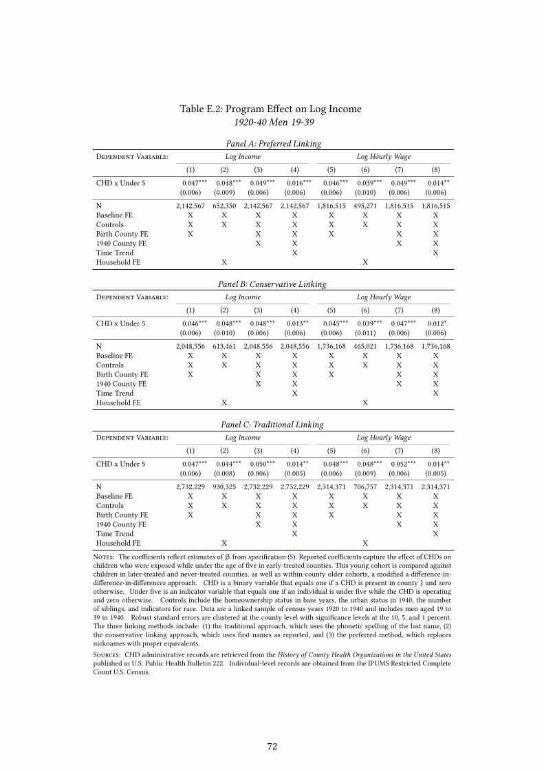
Table E.2: Program E�ect on Log Income1920-40 Men 19-39

Panel A: Preferred LinkingDependent Variable: Log Income Log Hourly Wage

(1) (2) (3) (4) (5) (6) (7) (8)

CHD x Under 5 0.047*** 0.048*** 0.049*** 0.016*** 0.046*** 0.039*** 0.049*** 0.014**(0.006) (0.009) (0.006) (0.006) (0.006) (0.010) (0.006) (0.006)

N 2,142,567 652,350 2,142,567 2,142,567 1,816,515 495,271 1,816,515 1,816,515Baseline FE X X X X X X X XControls X X X X X X X XBirth County FE X X X X X X1940 County FE X X X XTime Trend X XHousehold FE X X

Panel B: Conservative LinkingDependent Variable: Log Income Log Hourly Wage

(1) (2) (3) (4) (5) (6) (7) (8)

CHD x Under 5 0.046*** 0.048*** 0.048*** 0.013** 0.045*** 0.039*** 0.047*** 0.012*(0.006) (0.010) (0.006) (0.006) (0.006) (0.011) (0.006) (0.006)

N 2,048,556 613,461 2,048,556 2,048,556 1,736,168 465,021 1,736,168 1,736,168Baseline FE X X X X X X X XControls X X X X X X X XBirth County FE X X X X X X1940 County FE X X X XTime Trend X XHousehold FE X X

Panel C: Traditional LinkingDependent Variable: Log Income Log Hourly Wage

(1) (2) (3) (4) (5) (6) (7) (8)

CHD x Under 5 0.047*** 0.044*** 0.050*** 0.014** 0.048*** 0.048*** 0.052*** 0.014**(0.006) (0.008) (0.006) (0.005) (0.006) (0.009) (0.006) (0.005)

N 2,732,229 930,325 2,732,229 2,732,229 2,314,371 706,757 2,314,371 2,314,371Baseline FE X X X X X X X XControls X X X X X X X XBirth County FE X X X X X X1940 County FE X X X XTime Trend X XHousehold FE X X

Notes: The coe�cients re�ect estimates ofβ from speci�cation (5). Reported coe�cients capture the e�ect of CHDs onchildren who were exposed while under the age of �ve in early-treated counties. This young cohort is compared againstchildren in later-treated and never-treated counties, as well as within-county older cohorts, a modi�ed a di�erence-in-di�erence-in-di�erences approach. CHD is a binary variable that equals one if a CHD is present in county j and zerootherwise. Under �ve is an indicator variable that equals one if an individual is under �ve while the CHD is operatingand zero otherwise. Controls include the homeownership status in base years, the urban status in 1940, the numberof siblings, and indicators for race. Data are a linked sample of census years 1920 to 1940 and includes men aged 19 to39 in 1940. Robust standard errors are clustered at the county level with signi�cance levels at the 10, 5, and 1 percent.The three linking methods include: (1) the traditional approach, which uses the phonetic spelling of the last name, (2)the conservative linking approach, which uses �rst names as reported, and (3) the preferred method, which replacesnicknames with proper equivalents.Sources: CHD administrative records are retrieved from the History of County Health Organizations in the United Statespublished in U.S. Public Health Bulletin 222. Individual-level records are obtained from the IPUMS Restricted CompleteCount U.S. Census.

72

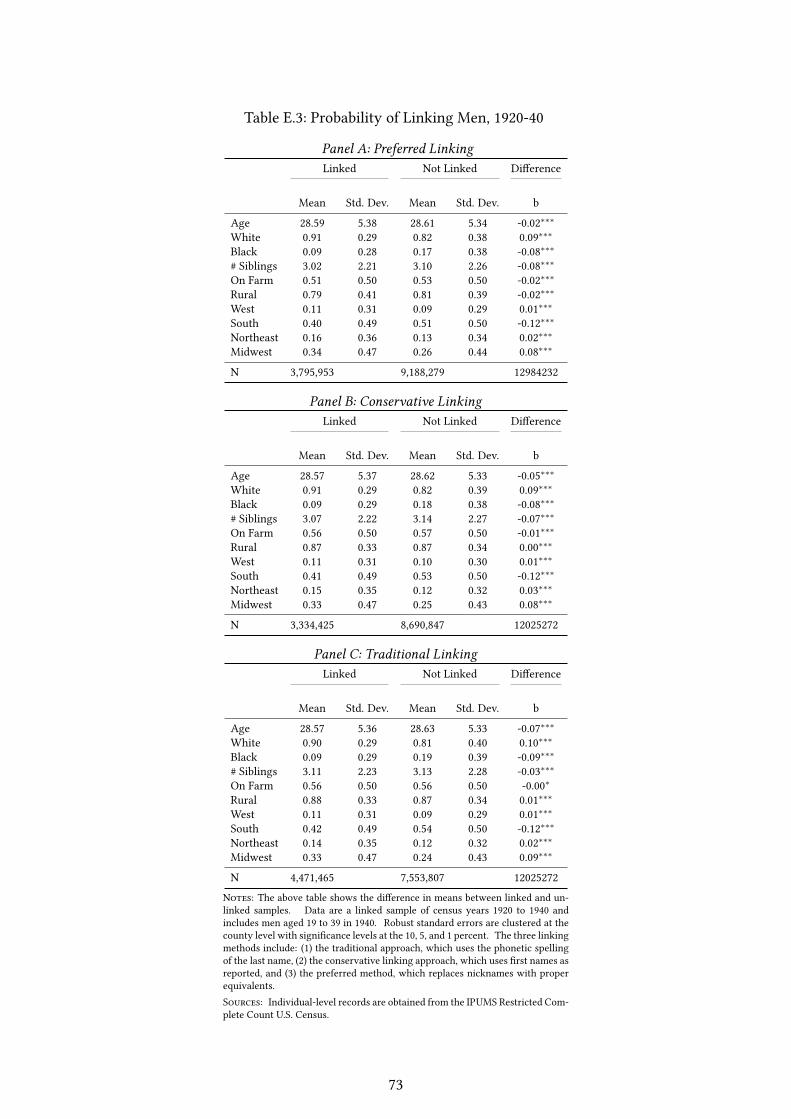
Table E.3: Probability of Linking Men, 1920-40

Panel A: Preferred LinkingLinked Not Linked Di�erence

Mean Std. Dev. Mean Std. Dev. b

Age 28.59 5.38 28.61 5.34 -0.02∗∗∗White 0.91 0.29 0.82 0.38 0.09∗∗∗Black 0.09 0.28 0.17 0.38 -0.08∗∗∗# Siblings 3.02 2.21 3.10 2.26 -0.08∗∗∗On Farm 0.51 0.50 0.53 0.50 -0.02∗∗∗Rural 0.79 0.41 0.81 0.39 -0.02∗∗∗West 0.11 0.31 0.09 0.29 0.01∗∗∗South 0.40 0.49 0.51 0.50 -0.12∗∗∗Northeast 0.16 0.36 0.13 0.34 0.02∗∗∗Midwest 0.34 0.47 0.26 0.44 0.08∗∗∗

N 3,795,953 9,188,279 12984232

Panel B: Conservative LinkingLinked Not Linked Di�erence

Mean Std. Dev. Mean Std. Dev. b

Age 28.57 5.37 28.62 5.33 -0.05∗∗∗White 0.91 0.29 0.82 0.39 0.09∗∗∗Black 0.09 0.29 0.18 0.38 -0.08∗∗∗# Siblings 3.07 2.22 3.14 2.27 -0.07∗∗∗On Farm 0.56 0.50 0.57 0.50 -0.01∗∗∗Rural 0.87 0.33 0.87 0.34 0.00∗∗∗West 0.11 0.31 0.10 0.30 0.01∗∗∗South 0.41 0.49 0.53 0.50 -0.12∗∗∗Northeast 0.15 0.35 0.12 0.32 0.03∗∗∗Midwest 0.33 0.47 0.25 0.43 0.08∗∗∗

N 3,334,425 8,690,847 12025272

Panel C: Traditional LinkingLinked Not Linked Di�erence

Mean Std. Dev. Mean Std. Dev. b

Age 28.57 5.36 28.63 5.33 -0.07∗∗∗White 0.90 0.29 0.81 0.40 0.10∗∗∗Black 0.09 0.29 0.19 0.39 -0.09∗∗∗# Siblings 3.11 2.23 3.13 2.28 -0.03∗∗∗On Farm 0.56 0.50 0.56 0.50 -0.00∗Rural 0.88 0.33 0.87 0.34 0.01∗∗∗West 0.11 0.31 0.09 0.29 0.01∗∗∗South 0.42 0.49 0.54 0.50 -0.12∗∗∗Northeast 0.14 0.35 0.12 0.32 0.02∗∗∗Midwest 0.33 0.47 0.24 0.43 0.09∗∗∗

N 4,471,465 7,553,807 12025272

Notes: The above table shows the di�erence in means between linked and un-linked samples. Data are a linked sample of census years 1920 to 1940 andincludes men aged 19 to 39 in 1940. Robust standard errors are clustered at thecounty level with signi�cance levels at the 10, 5, and 1 percent. The three linkingmethods include: (1) the traditional approach, which uses the phonetic spellingof the last name, (2) the conservative linking approach, which uses �rst names asreported, and (3) the preferred method, which replaces nicknames with properequivalents.Sources: Individual-level records are obtained from the IPUMS Restricted Com-plete Count U.S. Census.

73

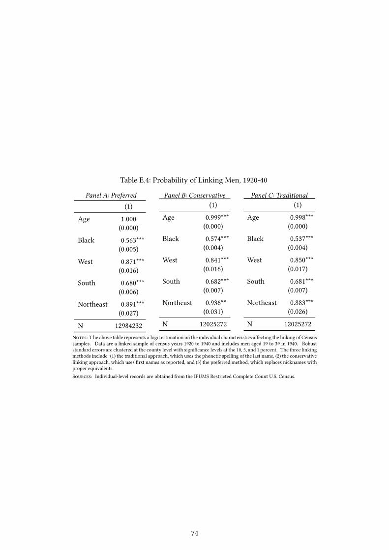
Table E.4: Probability of Linking Men, 1920-40

Panel A: Preferred

(1)

Age 1.000(0.000)

Black 0.563***(0.005)

West 0.871***(0.016)

South 0.680***(0.006)

Northeast 0.891***(0.027)

N 12984232

Panel B: Conservative(1)

Age 0.999***(0.000)

Black 0.574***(0.004)

West 0.841***(0.016)

South 0.682***(0.007)

Northeast 0.936**(0.031)

N 12025272

Panel C: Traditional(1)

Age 0.998***(0.000)

Black 0.537***(0.004)

West 0.850***(0.017)

South 0.681***(0.007)

Northeast 0.883***(0.026)

N 12025272

Notes: T he above table represents a logit estimation on the individual characteristics a�ecting the linking of Censussamples. Data are a linked sample of census years 1920 to 1940 and includes men aged 19 to 39 in 1940. Robuststandard errors are clustered at the county level with signi�cance levels at the 10, 5, and 1 percent. The three linkingmethods include: (1) the traditional approach, which uses the phonetic spelling of the last name, (2) the conservativelinking approach, which uses �rst names as reported, and (3) the preferred method, which replaces nicknames withproper equivalents.Sources: Individual-level records are obtained from the IPUMS Restricted Complete Count U.S. Census.

74

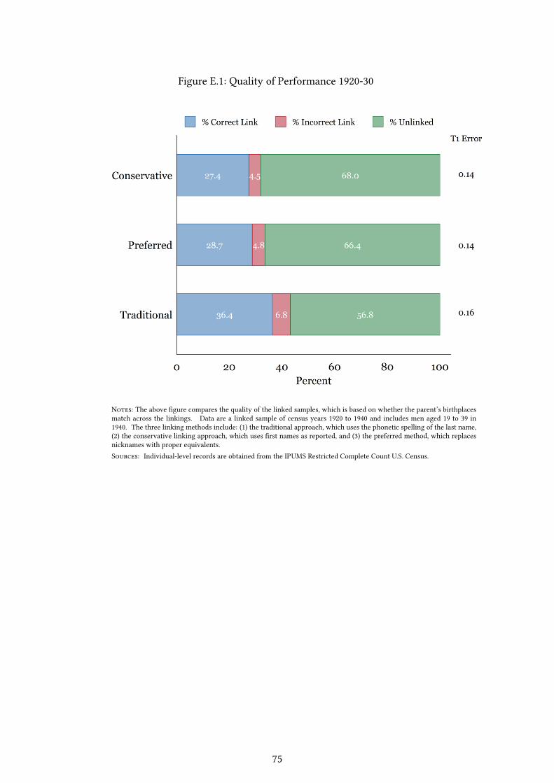
Figure E.1: Quality of Performance 1920-30

Notes: The above �gure compares the quality of the linked samples, which is based on whether the parent’s birthplacesmatch across the linkings. Data are a linked sample of census years 1920 to 1940 and includes men aged 19 to 39 in1940. The three linking methods include: (1) the traditional approach, which uses the phonetic spelling of the last name,(2) the conservative linking approach, which uses �rst names as reported, and (3) the preferred method, which replacesnicknames with proper equivalents.Sources: Individual-level records are obtained from the IPUMS Restricted Complete Count U.S. Census.

75