Embed Size (px)
Citation preview

THE LONG-TERM EFFECTS OF YOUTH UNEMPLOYMENT
Thomas A. Mroz¤ Timothy H. Savage∗
July 2003
Abstract Using National Longitudinal Survey of Youth data on young men, we estimate the long-term effects of youth unemployment on later labor market outcomes. A spell of involuntary unemployment can lead to sub-optimal investments in human capital among young people in the short run. A theoretical model of dynamic human capital investment predicts a rational “catch-up” response to such a spell. Using semiparametric techniques to control for the endogeneity of prior behaviors, our estimates provide strong evidence of this response. We also find evidence of persistence in unemployment. Despite the catch-up response, however, we find the negative effect of prior unemployment on earnings to be large, to be persistent and to taper off slowly over time. The theoretical model predicts each of these three effects. Combining our semiparametric estimates with a dynamic approximation to the lifecycle, we find that unemployment experienced as long ago as ten years continues to affect earnings adversely.
¤ Department of Economics, The University of North Carolina at Chapel Hill and The Carolina Population Center. Email: [email protected]. ∗ Charles River Associates. Email: [email protected]. We are grateful to Donna Gilleskie and David Guilkey for their valuable comments on prior drafts of this paper. We thank Brian Surette for his FORTRAN programs. Tetyana Shvydko provided excellent research assistance. Many useful comments on earlier drafts came from seminars at Duke, UNC, the Stanford Institute for Theoretical Economics, the World Bank, the Federal Reserve Bank of New York, and the University of Iowa. The Employment Policy Institute provided partial funding for this research project.

I. INTRODUCTION
The long-term effects of youth unemployment on later labor market outcomes are
critical factors in the evaluation of government policies that affect the youth labor market.
Adverse impacts may take the form of lower levels of human capital, reduced wage rates
and weakened labor force participation in the future. If these adverse effects are large
and persist through time, policies such as raising the minimum wage or increasing
unemployment benefits could have sizeable but hidden costs. Most analyses of the
potential impacts of labor market policy, however, focus only on contemporaneous
employment effects. This focus may be quite shortsighted, particularly for young people.
This research presents policy-relevant estimates of the effects of youth
unemployment on labor market outcomes later in life. We jointly model the endogenous
schooling, training, and labor market decisions and outcomes of young men over time
using a sample from the 1979 National Longitudinal Survey of Youth (NLSY79). The
econometric framework used in this study includes detailed controls for the endogeneity
of a wide range of human capital behaviors, including prior unemployment.
A spell of unemployment can lead to sub-optimal investments in human capital
among young people in the short run. A general dynamic model of human capital
investment and accumulation predicts a rational “catch-up” response to an involuntary
unemployment spell. The estimates presented here provide strong evidence of this catch-
up response. We find that recent unemployment has a significant positive effect on
whether a young man trains today. While there is little evidence of significant long-lived
persistence of unemployment spells on the incidence and duration of future
unemployment spells, there is short-term persistence.
1

Despite this catch-up response and an absence of long-lived persistence in
unemployment spells, there is evidence of long-lived “blemishes” from unemployment.
Dynamic simulations using our approximation to the lifecycle optimization process
indicate that a six-month spell of unemployment experienced at age 22 would result in
eight percent lower wages, on average, at age 23. This wage effect occurs whether we
“assign” unemployment to all working individuals in the sample or if we use increases in
local unemployment rates to induce those most at risk of layoff into unemployment. The
former scenario represents a “population average” effect, while the latter is a form of a
local-average treatment effect. Wages remain over five percent below their non-
disturbed level through age 26, and even at ages 30 and 31 wages are two to three percent
lower than they otherwise would have been. In 2002 US dollars at 2,000 hours per year,
a six-month spell of unemployment at age 22 yields a $1,400 to $1,650 earnings deficit at
age 26 (about six percent) and a $1,050 to $1,150 deficit (about four percent) at age 30, at
depending on the type of average effect one considers.
The remainder of this paper is divided into five sections. The next section
examines the existing literature on the long-term effects of youth unemployment. The
third section presents a simple analytic model of human capital accumulation that yields
several interesting propositions about unemployment, training and potential earnings.
The fourth section presents an empirical framework to analyze this issue and the data
used in this study. The fifth section discusses the estimation results derived from the
empirical model. The sixth section concludes.
2

II. PRIOR LITERATURE
Between 1969 and 1979, the unemployment rate of young people age 16 to 19 in
the US had risen by over 30% from 12.2 to 16.1 percent. At the time, policy-makers
feared that the nation was gripped by an unemployment problem that would
“permanently scar” the unemployed young.1 Therefore, early empirical analyses of the
long-term effects of youth unemployment focused on the extent to which early
unemployment spells affected the incidence and duration of future spells.2 These
analyses found evidence of strong persistence in unemployment.
In contrast, later studies drew a distinction between true state dependence and
unobserved heterogeneity.3 Hypothesizing that individuals differ in certain unobserved
characteristics, these studies demonstrated that a failure to control for heterogeneity
might spuriously indicate causal persistence. If such characteristics are correlated over
time, measures of state dependence act as proxies for this serial correlation in the absence
of suitable controls. Young people with weak preferences for work, for instance, will
tend to work less over time other things equal. Observed variables such as prior
unemployment are, therefore, statistically endogenous in regression analyses, and
unbiased measures of their effects on future spells cannot be obtained.
1 Policy-makers accorded much less importance, however, to the fact that the labor force participation rate for this age group had also risen considerably from 49.4 to 57.9 percent. To contrast the 16.1% rate in 1979, the US unemployment rate for 16- to 19-year-olds was 18.5% in May 2003, which is three times higher than the rate of the above-20 population. For black teenagers, the unemployment rate was over 37% at this time. 2 See Stevenson (1978) and Becker and Hills (1980). These studies viewed youth unemployment as involuntary. They predicted dire consequences for those young people who experienced unemployment early in their working lives. On the other hand, dual labor market theorists held that early unemployment would permanently track young people into jobs with low pay and little room for advancement. Drawing on the human capital models of Ben-Porath (1967) and Blinder and Weiss (1976), other analyses posited that early spells would deprive the young of labor force experience during that portion of the lifecycle when it yields the highest return. As a result, the lifetime earnings profiles of unemployed youths would permanently shift down. 3 See Heckman (1979), Heckman and Borjas (1980), and Flinn and Heckman (1981).
3

A 1982 National Bureau of Economic Research (NBER) volume on the youth
labor market approached the subject of youth unemployment, in part, by drawing on the
search-theoretic framework of Mortensen (1970) and Lippman and McCall (1976).
Many of the analyses in this volume posit that an extensive process of mixing and
matching among workers and firms characterizes the youth labor market. Young people
change jobs frequently due to low reservation wages and low opportunity costs. High
turnover rates, possibly punctuated by unemployment spells, are a natural characteristic
of this market and, as such, are not a source of concern.4
Within the context of this analysis, three of these papers require further
discussion. First, Corcoran (1982) examines persistence in employment status by
examining whether current employment status is influenced by prior employment status.5
She finds the odds that a young woman works this year are nearly eight times higher if
she worked last year than if she did not. Corcoran also examines the effect of prior
education and work experience on hourly earnings, finding that both positively affect
wages for the first few years out of school.6 Second, Ellwood (1982) examines
persistence in employment patterns using annual weeks of unemployment and annual
weeks worked.7 After controlling for unobserved heterogeneity with a fixed-effects
specification, he finds no persistence in unemployment and slight evidence of persistence
in work behavior. He also examines the effect of prior education and work experience on
hourly earnings, finding that both have a significant and positive effect for the first few
4 See Freeman and Medoff (1982) and Freeman and Wise (1982). 5 With a sample of young females from the National Longitudinal Survey of Young Women, she uses the Chamberlain’s (1980) conditional logit model. Chamberlain (1984, pp 1274-1278), however, notes that this specification is not consistent in this context because it assumes that there is no occurrence dependence, which is exactly what Corcoran is measuring. 6 The sample is young women from the Population Study of Income Dynamics who have finished school. 7 The sample is young males from the National Longitudinal Survey of Young Men.
4

years out of school. In both the Corcoran and Ellwood studies, the cost of forgone
participation appears to be lower future wages rather than persistent nonparticipation in
the labor market.8 Third, using normal maximum likelihood methods to control for
endogeneity, Meyer and Wise (1982) jointly model the choices of schooling and annual
weeks worked. They also jointly model the schooling decision and wages. They find
that hours of work during high school positively affect weeks worked after graduation
and that early labor force experience positively affects wages. They jointly model only
two of the several outcomes of interest, however. While they recognize that schooling,
experience and wages should be modeled and estimated jointly, they leave this task to
future research.9
There are several other papers that fit within the context of this research.10
Michael and Tuma (1984) examine the labor market effects of early labor force
experience.11 Regressing wages and schooling on lagged experience, they find that early
employment does not affect wages or schooling likelihood two years later. They treat
early experience as exogenous, however, and do not control for possible unobserved
heterogeneity. Ghosh (1994), who treats early decision-making as exogenous, also
8 If unobserved tastes vary as young people age, however, neither of these studies controls appropriately for unobserved heterogeneity. Variables such as schooling or prior unemployment remain endogenous, and estimates of their effects on outcomes such as hourly earnings are biased. Furthermore, evidence (Lewis [1986] and Robinson [1989]) indicates that the fixed-effects specification exacerbates problems of measurement error in a manner that biases estimates toward zero. 9 Since their data omit high school dropouts, young people for whom early unemployment may have large effects later in life, their results could under-state the true long-term effects of early unemployment. Further, recent Monte Carlo evidence (Mroz and Guilkey [1992] and Mroz [1999]) indicates that the normality assumption, when invalid, often induces greater bias than ignoring the endogeneity in models of the type used by Meyer and Wise. 10 See also Lynch (1985), Lynch (1989), Narendranathan and Elias (1993), Raphael (1996), and the Report on the Youth Labor Force by the US Department of Labor (2000). 11 The sample is 14- and 15-year-olds from the NLSY79. While this age range may appear quite young, they note that a quarter of the male sample works on average 12 hours per week.
5

examines the effects of early labor force experience.12 Using proxies such as test scores
to control for heterogeneity, he regresses hours worked and wages at ages 22 and 23 on
early schooling and experience and finds that early experience has positive long-run
effects on hours worked and wage rates. Finally, in a subsequent NBER volume on the
youth labor market, Card and Lemieux (2000) hypothesize that young people adapt to
changes in labor market conditions in a variety of ways.13 They find that weaker labor
market conditions and lower wages increase the likelihood that young men stay at home
with their parents, as well as remain in school. Their hypotheses, however, are not
ultimately tied directly to a formal model of optimization under uncertainty.
In summary, much of the current literature on the long-term effects of youth
unemployment contains shortcomings. These include: the use of small or non-random
samples; the failure to control adequately for unobserved heterogeneity and endogeneity;
insufficient time horizons to evaluate the full impacts of early unemployment; the
imposition of unnecessarily restrictive statistical assumptions; the lack of a theoretical
foundation; and, the absence of specific and meaningful policy conclusions.
This research addresses these deficiencies directly. It uses a large sample
representative of the young male US population in 1979. The labor market, schooling
and training decisions and outcomes of this sample are followed for 16 years. We jointly
model and estimate these outcomes using a permanent/transitory error-components
specification for unobserved determinants. This specification controls for the
contaminating effects of unobserved heterogeneity, self-selection, and endogeneity. We
12 His sample is 14- and 15-year-olds from the NLSY79. He specifies a recursive system whereby labor force participation (either a dummy variable or actual average hours of work) is influenced by exogenous characteristics and unobserved ability. Participation and unobserved ability affect the level of schooling, which in turn influences hours worked and separately wages at age 22 and 23.
6

test hypotheses arising from a model of maximizing behavior under uncertainty. The
estimates and simulations from this research can help one gauge the long-term impacts of
policies that affect the youth labor market.
13 The US sample is from the Current Population Survey. The Canadian sample is based on Canadian census data.
7

III. A CONCEPTUAL FRAMEWORK
Consider the following analytic model of human capital investment. The model is
similar to Ben-Porath’s (1967) classic model with the addition of random unemployment
shocks that affect one’s ability to earn and train.14 In this model, the present and the
future are linked through the process of human capital accumulation. An exogenous
shock that perturbs the optimal time-path of human capital investment in one period
persists through time via its effects on additions to the human capital stock. The model is
used to examine the effects of this shock on future behaviors and outcomes.
In this model, individuals live with certainty for T periods and may train in each
of the first T-1 periods.15 For the moment, assume, as in Ben-Porath, that there is no
unemployment. At the beginning of period t, an individual’s human capital stock is given
by . Individuals invest in additional human capital by devoting a fraction of their time,
, to human capital production, which we call training. Training occurs on the job and
is considered to be general. There are no savings, no human capital depreciation and no
decisions regarding hours of work other than the choice of the fraction of time to devote
to investments and away from current earnings. Potential earnings, , could be
obtained by renting the human capital stock at a constant rate w: .
tH
ts
*tE
= tt wHE * 16 It is
always possible to obtain these earnings, except when experiencing involuntarily
unemployment. Disposable income (or net earnings) is the difference between potential
14 Ben-Porath uses a continuous-time framework, while the model described here is in discrete time. Unlike Ben Porath, we do not allow the human capital production function to exhibit Harrod neutral technical change. See Appendix 1 for a complete presentation of this model. 15 Because training is costly and there is no future gain, it is optimal not to train in the last period. 16 As with Ben-Porath, there is an initial positive stock of human capital that is exogenous.
8
earnings and the opportunity cost of human capital used in the production process, or
. ttt wHsE )1( −=
)1( λ−
At the beginning of each period, an individual chooses the fraction of his time to
devote to the production of new human capital, . Human capital at the start of the next
time period is given by , where s is the actual amount of time that
ends up being devoted to producing new human capital. In the absence of
unemployment, s . We assume that the production function of human capital is
increasing in its argument and strictly concave. These investment choices through time
yield an optimal time-path of human capital investment and accumulation.
ts
)( *1 ttt sfHH +=+
t
*t
t s=*
We assume that all unemployment is involuntary and that individuals have
rational expectations about the probability of experiencing unemployment. The
probability of unemployment does not depend on the individual’s choice of . All
training and earnings for each time period take place on the single job chosen at the start
of the time period (indexed by the value of s ) before the individual’s unemployment
status is revealed. When unemployment strikes, it reduces disposable earnings and
optimally planned training time on the job by equal percentages. In particular, let
ts
t
be the fraction of the time period that the individual spends unemployed. If he
experiences unemployment, then his actual disposable earnings in the time period would
be tt wHs )1( −tE = λ , and the additions to the human capital stock during the period he
is unemployed would be given by )( tsf λ .17 Unemployment, therefore, perturbs an
17 A simple way to conceptualize this setup is to assume that at the start of the “year” an individual chooses a job for that entire year that allows him to devote the fraction s of each working day to producing new t
9

individual’s optimal time-path of human capital accumulation by preventing on-the-job
training. This results in an under-investment in human capital after the unemployment
spell occurs. One can view unemployment at time t, then, as an exogenous reduction in
the amount of human capital available at the start of period t + 1.
Those who experience an unemployment spell in the preceding period enter the
current period with a lower stock of human capital than otherwise identical individuals
who did not experience unemployment. Crucially, having experienced the shock,
individuals are able to re-optimize at the beginning of this next time period. This re-
optimization yields a new optimal time-path of human capital investment. Besides
lowering lifetime expected wealth, the only lasting effect of an involuntary
unemployment spell is that it constrains an individual to a lower human capital
accumulation than he had planned. This model, therefore, can be used to examine the
spell’s effect on future behaviors. It can also used to examine how a spell affects
observable outcomes such as earnings and training, and it provides a mechanism through
which these effects may be mitigated by optimal behavioral responses. The model
provides three interesting implications.18
Proposition 1: The “Catch-up” Response
After experiencing an involuntary unemployment spell in all years except T and T-1, an
individual will unambiguously increase the time that is spent training in the next period.
This proposition states that a young person will exhibit an optimal “catch-up”
response to an involuntary unemployment spell that exogenously reduces his human
capital acquisition at time t. An exogenous spell perturbs a young person’s optimal time-
%human capital. If unemployment occurs, the individual loses the latter 100 of the year’s workdays for
earning disposable income and for producing human capital. λ⋅
10

path of human capital investment. Re-optimization that takes the spell into account,
however, yields a new optimal time-path for the human capital investments. This re-
optimization produces an unambiguous effect on future behavior: a young person will
increase the share of time that is spent training.19 We refer to this change in subsequent,
optimal investment choices as a “catch-up” response.
Proposition 2: The Convergence of Potential Earnings
The effect of the unemployment spell on potential earnings diminishes over time.
This proposition states that, because of the optimal response to the human capital
shock, the compensatory training behavior results in a convergence in the unperturbed
and perturbed human capital stocks. Therefore, the behavior directly mitigates the
unemployment spell’s effect on potential earnings over time. This model demonstrates
persistence in the sense that the effect of a spell in a single period lasts beyond that
period. Optimizing behavior, however, mitigates that effect over time.
Proposition 3: Excessive Divergence Followed by Excessive Convergence of
Disposable Earnings
Observed net earnings immediately after experiencing unemployment are lower than
would be implied by solely the reduction in the human capital stock. Furthermore,
observed earnings grow faster after the first period following an unemployment spell
than would be implied by the convergence of the human capital stocks.
This proposition states that, observed differences in disposable earnings between
those who were and those who were not recently unemployed are larger than would be
18 See Appendix 1 for proof of these propositions. 19 An alternative view of this “catch-up” response is that those who did not experience unemployment had acquired “too much” human capital at time t because they did not become unemployed. They in turn reduce their production of new capital at t+1.
11

implied by the differences in their human capital stocks. To see this, holding fixed the
share of time that is spent training, the reduction in earnings would reflect exactly the
lower stock of human capital. The optimal catch-up response, however, implies that a
recently unemployed individual increases the share of time that is spent training.
Therefore, he necessarily decreases the share of time spent producing disposable
earnings, which results in observed earnings that are lower than would be implied solely
by the reduction in the human capital stock.
In subsequent time periods, because of the catch-up response, the gap in human
capital stocks diminishes between those who had and had not experienced
unemployment. Differences in the shares of time spent training, therefore, become less
pronounced. The later convergence of disposable earnings reflects both the convergence
of the human capital stocks as well as the convergence of the human capital investment
decisions.
This is conceptual model is simple but useful. It directly links the present and the
future through the process of human capital investment and accumulation. By positing
equivalence between an involuntary unemployment spell and an exogenously constrained
human capital stock, one can examine the effects of such unemployment on future
behavior and outcomes.20 In our empirical analysis, we assume that observed hourly
wages are net of human capital training costs. Wage rate differentials reflect both
differences in human capital stocks and differences in the amount of time spent in on-the-
job training.
20 This model does not address job search or time voluntary spent not working. These and other limitations are discussed in Appendix 1.
12

IV. THE EMPIRICAL SPECIFICATION AND THE DATA
The chief goal of this research is to provide policy-relevant predictions of the
long-term effects of youth unemployment on future labor market outcomes. The
preceding conceptual model provides a link between prior unemployment and future
behaviors and outcomes through the human capital accumulation process. In this model,
an exogenous unemployment spell results in sub-optimal human capital acquisition that
directly affects future decisions and outcomes. Here we address crucial econometric,
data, and empirical issues.
We jointly model the endogenous schooling, training, and labor market decisions
and outcomes of young people over time. Each year, a young person chooses whether to
train, to attend school, and to participate in the labor market. Conditional on his labor
force participation, he chooses how many hours to work annually. A young man may
also experience unemployment, either voluntary or involuntary, during the year. Hourly
earnings as well as schooling, training, and labor force participation may be affected by
the unemployment. We jointly estimate this system of equations using the
semiparametric, full-information maximum likelihood method suggested for single
equations by Heckman and Singer (1984) and extended to simultaneous equations by
Mroz and Guilkey (1992) and Mroz (1999). This discrete factor maximum likelihood
(DFML) method allows complex correlation across equations and over time. It explicitly
models and controls for the contaminating effects of heterogeneity and endogeneity.
By using this procedure, we are able to control effectively for the endogeneity of
a wide range of the youths’ previous decisions and outcomes on their later behaviors and
outcomes. For example, we are able to model a wide range of endogenous behavioral
13

determinants including previous unemployment, job changing, schooling, and work
experience. The estimates reported in this study, then, should be interpreted as the
impacts of an exogenously induced change in the endogenous determinants.
Furthermore, by controlling for endogeneity for this wide range of employment, training,
and wage determinants, the estimates reported here should provide more relevant
predictions for policy evaluations than those found in previous studies of the impacts of
youth unemployment.
Modeling the Outcomes of Interest
In a study of this type, there are many potentially endogenous human capital
variables that are used as explanatory variables. They include the stocks of education and
work experience, as well as prior unemployment. In addition, there are potential self-
selection issues for the observed working and training outcomes. To account for these
potential sources of bias, up to eight behavioral outcomes are jointly modeled every year
for each young person in the sample. These outcomes are (log) average hourly earnings;
whether or not a young man works; annual hours worked if working; whether or not a
young man is unemployed; annual weeks of unemployment if unemployed; whether the
individual changed jobs; school attendance; and training. We also specify an initial
condition equation to control for the endogeneity of each person’s schooling attainment at
the start of the panel.
Log average hourly earnings are specified to be Mincer-type earnings functions.
They depend upon polynomials in age and in cumulative work experience, the stock of
14

education and demographic variables.21 Hourly earnings may also be affected by prior
unemployment.22 We also allow hourly earnings to be affected by recent job changes in
order to separate out the effects of experiencing unemployment from those attributable to
just changing one’s employer. We allow for up to five annual lags for weeks spent
unemployed and for job changes.
Annual hours of work depend upon local labor market conditions, polynomials in
age and in labor force experience, education, prior unemployment and demographic
variables. Annual weeks of unemployment depend upon local labor market conditions,
polynomials in age and in labor force experience, education, prior unemployment and
demographic variables. Training is a dummy variable that takes the value one if a young
person took part in any government-sponsored or vocational training in a particular
year.23 It depends upon polynomials in age and in labor force experience, education,
local labor market conditions, demographic variables and five years of unemployment
and job change histories. Schooling is a dummy variable that takes the value one if a
young person participated in any secondary or post-secondary education in a particular
year. It depends upon polynomials in age and in labor force experience, demographic
variables, and prior unemployment. Each of these equations also includes four time
period dummies (for 1979, 1980 to 1982; and 1992 to 1994, with 1983-1991 being the
21 The stock of education is measured by highest grade completed, whether a young man possesses a high diploma or a general equivalence degree (GED) and whether he possesses a four-year college degree. 22 If the mechanism through which unemployment affects wages is exclusively forgone human capital, there should be no effect of prior unemployment on wages after perfectly controlling for the human capital stock. Perfectly controlling for the human capital is unlikely, however, because the human capital variables are only proxy measures. 23 The NLSY79 questionnaire was altered in 1987 when its management was transferred to the Bureau of Labor Statistics (BLS), and no training questions were asked in this year. In 1988, the questionnaire asked whether any training had occurred either in 1987 or 1988.
15

excluded category). Complete specifications for all equations, along with point estimates
and standard errors, are reported in Appendix 2.
The Likelihood Function
To derive the likelihood function for the system of equations to be estimated, we
use the following observed sequence for each young person i in each year t:
{isi, asit, trit, workit, hwit, unit, wuit, chit, wit} where:
isi is initial schooling at the start of the NLSY79 survey
asit is a dummy variable for school attendance in year t
trit is a dummy variable for any vocational training in year t
workit is a dummy variable for working in year t
hwit is hours worked during year t (if working)
unit is a dummy variable for experiencing unemployment in year t
wuit is the number of weeks unemployed in year t (if unemployed)
chit is a dummy variable indicating a job change in year t
wit is the logarithm of average hourly earnings in year t (if working)
Let εit be a vector with nine elements that contain unobserved determinants of the
above outcomes. These unobserved determinants are specified to have an error-
component structure: ititiit u +η+ρµ=ε , where ρ is a matrix of factor loads and µi is a
vector of unobserved factors. This represents a permanent/transitory error specification.
Assume uit is a mean-zero iid normal error vector. The primary substantive restriction
this error-components structure places on the density of εit is that all correlation across
16

equations in different time periods enters solely through the linear factors µi . Within time
periods, the covariance pattern is unrestricted due to the freely-estimated relationships
among the elements of ηit, though we do impose that the joint distribution does not vary
through time. The factors µi capture unobserved determinants that do not vary as young
people age such as, perhaps, ability.24 The factor ηit captures time-specific unobserved
determinants that may vary across time such as preferences for work.25 It allows for
arbitrary, contemporaneous correlation of outcomes at each point in time that is not
captured by the person specific unobserved factor.
As an example of a discrete outcome, consider training, trit. As with the other
four dummy variable outcomes modeled in this study, a latent index specification is used.
otherwise 0 and 0 if 1 trwhere
'
*it
,,
5
1,
5
1,,
*
=>=
+++++′= ∑∑=
−=
−
it
ittrittritritchittrtrittrit
tr
uchwuxtr ηµργβατ
τττ
ττ Equation 1
At each point in time, a young man trains if the value of his latent index is positive. The
decision to train is influenced by a vector of observed variables, xtr,it. This vector of
variables, briefly discussed earlier, includes background characteristics together with
demographic and (potentially endogenous) human capital variables.26 This decision is
also influenced by permanent and transitory factors that are not observed. Crucially, the
decision to train is also influenced by prior unemployment and prior job changes for up to
24 The error structure for initial schooling is modeled only with the permanent heterogeneity factors. 25 This specification we use is linear in two permanent heterogeneity factors and is nonlinear in the transitory heterogeneity factor. 26 These variables are listed in Tables 1 and 2 in the data section and in Appendix 2.
17

five years.27 This study focuses on the estimates of the β’s, the impacts of prior
unemployment, for each of the eight outcomes:
1,...,5 τand wch, wu,un,hw,work,tr,as,ofor β τo, == .
As an example of a continuous outcome, consider annual hours worked.28
hithitihitchithhhitit uchwuxh +++++′= ∑∑=
−=
− ηµργβατ
τττ
ττ '5
1,
5
1, Equation 2
Every year for each young man, annual hours of work are influenced by a vector of
observed variables and unobserved error terms. As with the other outcomes, hours of
work are also influenced by prior unemployment and job changes for up to five years.
A researcher can control for the contaminating effects of heterogeneity and
endogeneity by integrating out the unobserved factors, µi and ηit. For example, if the
factors were normally distributed, one could use multivariate normal maximum
likelihood. The discrete factor integration method used in this study assumes that the
underlying continuous distributions of the factors can be suitably approximated by
discrete distributions with mass points and probability weights that are estimated jointly
with the other parameters in the system. Integration is greatly simplified since it requires
only summing the suitably weighted products of density functions and univariate
integrals. Further, the researcher does not have to make a priori assumptions about the
distribution of the factors since the discrete approximation is driven by the data.
Conditional upon the factors, the contribution to the likelihood of individual i in
year t is:
27 The choice of a five-year lag structure is somewhat arbitrary. There is some evidence that unemployment longer ago than five years is influential for one outcome.
18

{ }{ }{ }[ ] { }{ }[ ] { }{ } { }{ } { } )1(
)1(
)1(
)1(
)1(
,|0Pr,|1Pr
,|0Pr,|1Pr
,|0Pr),|(,|1Pr
,|0Pr),|(),|(,|1Pr
,|0Pr
,|1Pr),|(
itit
it
itit
itit
itit
it
tritiit
tritiit
as
chitiit
chitiit
unitiit
unitiitwunitiit
workitiit
workitiitwitiithitiit
itiit
asitiititiit
trtr
chch
unwunfun
workwfhfwork
as
asL
−
−
−
−
−
=⋅=
=⋅=
⋅=⋅⋅=
⋅=⋅⋅⋅=
⋅=
⋅==Θ
ηµηµ
ηµηµ
ηµηµηµ
ηµηµηµηµ
ηµ
ηµηµ
⋅ Equation 3
where fh is the annual hours worked density, fw is the log wage density, fwu is the annual
weeks unemployed density, and Θ is a vector of parameters to be estimated.
Approximating the distributions of µi and ηit with mass points µ1j, for j = 1,…,J,
µ2k, for k = 1,…,K, and ηm (vector) for m = 1,…,M, the contribution to the likelihood
function of individual i is:
( )
{ } { } ,for Pr ,2,1andfor Pr where
),,|(),|(),(
83
1 1 1213212
11
RpgRp
LpisfppL
mmimgrgrgigr
K
k
T
t
M
mmkjitmkjiisk
J
jji
∈===∈==
Θ⋅=ΓΘ ∑ ∏∑∑= = ==
ηηηµµµ
ηµµµµ
fis is the density for the potentially endogenous initial condition describing schooling
completed at the start of the longitudinal survey, and Γ is the vector containing the
parameters of the discrete distributions.
Identification
This study treats training, school attendance, work experience, prior job changes,
and unemployment as potentially endogenous variables that evolve as the young men in
the sample age. The dynamic structure of this model secures the identification of the
28 The decision to work, wages and unemployment are modeled only for those young men not in school. Further, annual hours of work and wages are modeled only if a young man chooses to work, while weeks of unemployment are modeled only for those who experience a spell of unemployment during the year.
19

effects in ways that cannot be achieved in static analyses.29 Within this dynamic
structure, lagged exogenous variables satisfy the conditions for instrumental variables.
To see this, consider the unemployment rate in the local labor market. At any point in
time, such a variable is exogenous to young people. In 1985, variation in this rate has a
direct impact on 1985 labor market choices. Similarly, variation in 1983 has a direct
impact on 1983 choices. Because of the timing of decision-making, however, the 1983
rate has no direct impact on 1985 decisions except through the accumulated stock of
human capital as of 1985. Consequently, the 1983 rate is an instrumental variable in
1985. This argument, of course, applies to different years and to the other exogenous
variables in this study. Therefore, there are numerous “instruments” available, and the
dynamic maximum likelihood procedure allows these to be exploited efficiently.
Identification in this model is also secured with theoretical exclusion restrictions
and through non-linearities in the likelihood function. Variables described later in this
section that use exogenous state-level data provide these theoretical exclusion
restrictions. These variables directly affect the schooling and training decisions and labor
supply, but have no direct impact on wages other than through the human capital stock.
They are, therefore, excluded from the wage equation.
Alternative Approaches to Estimation
To assess some of the more important findings in this paper, we also use more
standard single-equation approaches to estimate the impact of prior unemployment on
29 For a more thorough discussion of identification in models of this type, see Mroz and Surette (1998).
20

particular outcomes of interest.30 For the most part, these alternative approaches provide
estimates that are qualitatively similar to those from the discrete factor maximum
likelihood approach, and in only one instance do we find evidence of significant
differences between the fixed-effect estimates and the DFML estimates. It is important to
note that for the labor market and schooling outcomes that we examine, there could be
potentially serious sample selection biases. In most instances, only the DFML estimator
has the potential to control for such selection biases when compared to the single-
equation approaches. Further, since much of our analysis explicitly deals with
moderately complex patterns of prior outcomes influencing current outcomes through the
process of human capital accumulation, one should discount the relevance of the
conditional/fixed-effect logit estimates presented here. Such estimators can exhibit
considerable bias when the outcome of interest depends on prior outcomes for the
process.31
The Data
The primary data for this research are taken from the 1979 National Longitudinal
Survey of Youth (NLSY79) and its geocode supplement. We use young men who were
14 to 19 years old in 1979 and are drawn from both the representative sample and the
over-samples of blacks and Hispanics. This yields a sample size of 3,731, of which 2,286
are from the representative sample and 1,145 are from the two over-samples. We follow
these young men through 1994. When constructing this sample, we applied the following
30 For continuous dependent variables, these are ordinary least squares (OLS) and fixed-effect regressions. For discrete dependent variables, these are probit and Chamberlain’s (1980) conditional/fixed-effect logit. 31 See Chamberlain (1984, pp 1274-1278).
21

two selection criteria.32 First, a young man remains in the sample until his first non-
interview date, after which he leaves the sample regardless of whether he is interviewed
at some future date.33 Second, those young men not in the initial military sub-sample
who enter the armed forces permanently leave the sample upon entry.34
Table 1 contains variable descriptions and summary statistics for the time-
invariant characteristics of our sample. The first column of numbers contains the sample
means for the entire sample. The next two columns contain the means for the
representative and over-sample portions respectively. The variable afqt is derived from
the 1980 Armed Forces Qualification Test (AFQT).35 The scores from this test are
regressed against age dummies to purge pure age effects.36 Each value is then mean-
differenced using the mean for the entire sample.
The first eight rows of Table 2 contain the unweighted means for the entire
sample in 1979, 1986 and 1993 of the outcomes that are jointly modeled in this study. As
shown in Figure 1, average annual weeks of unemployment appear quite anti-cyclical
over this 16-year period, peaking in the recessions of the early 1980s and early 1990s.
Figure 1 shows averages both for the entire sample and conditional upon any
unemployment during the year. Average school attendance declines monotonically
throughout the 16-year period. Average participation in vocational training rises to a
32 By 1986, these selection criteria affect nearly 25% of the sample. By 1994, nearly 40% is affected. 33 The average length of a non-interview spell is greater than three years. Given the age of this sample, the failure to observe outcomes for this length of time could induce bias in estimates of interest. If the attrition process is random, this selection procedure does not bias the estimates. See MaCurdy, Mroz and Gritz (1998) for a detailed analysis of attrition from the NLSY. 34 Despite the role that training plays in the armed forces, those young men who enter the military report no training. 35 Approximately 90% of the original cohort was administered the AFQT test. 36 For those in my sample not administered the test, a predicted value is assigned using the race-specific mean residual from the age regression.
22

maximum of 18.0% in 1993 but declines slightly in 1994. Average annual hours of work
rise monotonically from 481 in 1979 to 2,034 in 1991. They decline somewhat in 1992
and 1993 but return to their 1991 level by 1994. Real average hourly earnings (in logs)
rise monotonically from 1979 to 1993.37 Training started out low in 1979, reflecting the
young age of the sample at that date. By 1993, over one in six young men reported some
type of formal vocational training. The remaining rows in Table 2 contain the time-
varying unweighted averages for other variables used in this study.
Table 1: Summary Statistics of Time-Invariant Characteristics (Standard Deviations Omitted for Dummy Variables) Variable Name
Variable Description
Entire (St. Dev.)3731 obs
Represent. (St. Dev.) 2286 obs
Over-sample (St. Dev.)1145 obs
Afqt Armed forces qualification test score 0.00 (28.13)
8.14 (28.35)
-12.88(22.40)
Initsch Initial level of schooling 9.64 (1.67)
9.75 (1.63)
9.45 (1.71)
Mohgc Mother's highest grade completed
10.86 (3.12)
11.60 (2.63)
9.68 (3.46)
Fahgc
Father's highest grade completed
10.96 (3.64)
11.90 (3.38)
9.46 (3.54)
readmat Age 14: Household received newspapers or magazines
0.81 0.89 0.69
Libcard
Age 14: Household had a library card 0.68 0.72 0.61
prot
Age 14: Young man raised protestant 0.50 0.50 0.49
Livpar
Age 14: Young man lived with both parents
0.67 0.75 0.55
Black
Black in random sample 0.07 0.11 0.00
Hispanic
Hispanic in random sample 0.05 0.07 0.00
Overblack
Over-sampled Black 0.24 0.00 0.69
Overhisp
Over-sampled Hispanic 0.15 0.00 0.31
37 Average hourly earnings are defined as total annual earnings from wages and salary divided by annual hours worked. They are deflated using the CPI-UX1 price index with a base year of 1982.
23

Table 2: Summary Statistics of Time-Variant Variables (Standard Deviations Omitted for Dummy Variables) Variable Name
Variable Desciption
1979 Mean(St. Dev.)3731 obs
1986 Mean (St. Dev.) 2805 obs
1993 Mean(St. Dev.)2304 obs
Un Dummy variable: Any unemployment during the year
0.30 0.29 0.19
Wun Annual weeks of unemployment (entire sample) 3.32 (8.00)
4.20 (9.75)
2.83(7.97)
Work Dummy variable: Any work during the year
0.58 0.93 0.93
Hw Annual hours worked (entire sample) 627.97 (776.92)
1814.14 (909.24)
2026.20(904.26)
Lnw Log of deflated average hourly earnings from wages and salary (in 1982 dollars)
1.31 (0.79)
1.76 (0.73)
2.02(0.66)
Anysch Dummy variable: Any schooling during the year
0.89
0.20
0.07
Train Dummy variable: Any training during the year
0.03
0.12 0.18
Chjob Dummy Variable: Change job in prior year
0.0027 0.1027 0.0660
age Age 16.55 (1.60)
23.54 (1.63)
30.52(1.63)
exp Cumulative labor force experience in hours/2000 0.24 (0.35)
4.39 (2.55)
11.29(4.35)
hgc Highest grade in years completed 9.64 (1.67)
12.51 (2.23)
12.96(2.54)
geddeg Dummy Variable: Holds a general equivalence degree
0.01
0.09 0.12
hsdeg Dummy Variable: Holds a high school diploma
0.15 0.66 0.69
coldeg Dummy Variable: Holds a four-year college degree
0.00 0.12 0.19
urb Dummy Variable : Residence is urban
0.80 0.82 0.81
ne Dummy Variable : Residence is Northeastern US
0.20 0.18 0.17
nc Dummy Variable : Residence is North-Central US
0.26 0.25 0.26
so Dummy Variable : Residence is Southern US
0.36 0.37 0.37
we Dummy Variable : Residence is Western US
0.19 0.20 0.20
ur Local labor market unemployment rate (in percent) 6.31 (1.97)
7.77 (2.84)
7.53 (2.60)
expsec Per-pupil public expenditure on secondary institutions (in 1982 dollars)
3107.27 (732.91)
3694.57 (930.58)
4056.55 (1042.62)
expps Per-pupil public expenditure on post-secondary institutions (in 1982 dollars)
5735.19 (1122.29)
6454.09 (1135.09)
6828.19 (1154.78)
ugtuit Annual undergraduate tuition at main or largest campus of state university (in 1982 dollars)
1142.54 (391.76)
1475.57 (540.10)
2067.79 (753.73)
Mw The larger of federal or state-level hourly minimum wage (in 1982 dollars)
3.93 (0.09)
3.07 (0.07)
2.97 (0.12)
24

02
46
810
1214
1618
Wee
ks o
f Une
mpl
oym
ent
79 80 81 82 83 84 85 86 87 88 89 90 91 92 93Year
Series with triangles is average conditional on any unemployment during the year.Series with diamonds is average for the entire sample.Source: NLSY79.
Figure 1: Average Annual Weeks of Unemployment
There are several sources of state-level data that are matched to the NLSY
sample. The first is data taken from the Digest of Education Statistics (DES) on per-
student public expenditure at public secondary education institutions. The second is DES
data on per-student public expenditure at post-secondary education institutions. The third
is data taken from the Integrated Post Secondary Education Data System (IPEDS) on
annual tuition prices at the largest or main campus of the state university system.38 These
expenditure and tuition data have been deflated using the CPI-UX1 deflator and show
substantial variation through time and across states. For example, in 1979 the New
England states spent nearly 25% more per-student on secondary education than southern
38 We are grateful to Alex Cowell for the tuition price data.
25

states, while tuition charges at public universities in the South were 80% lower than
charges in New England. By 1986, these differentials were 37% and 49% respectively.
Data on mandated minimum wages are also matched to the NLSY sample.
Because certain states, notably California, Massachusetts and Pennsylvania, often have
mandates that exceed the federal minimum, we use the larger of the federal or state
mandate. These data are also deflated and show considerable variation over time. As
shown in Figure 2, the real value in 1982 dollars of the federal minimum wage declined
by about 30% from 1979 to 1989, a period during which the federal mandate remained
unchanged. It rises in 1990 and 1991 due to legislated increases, but declines thereafter.
The real value of the minimum wage in 1991 is about 80% of its 1979 value.
2.5
2.7
2.9
3.1
3.3
3.5
3.7
3.9
4.1
1982
Dol
lars
79 80 81 82 83 84 85 86 87 88 89 90 91 92 93 94Year
Source: US Department of Labor and Bureau of Labor Statistics.
Figure 2: Real Value of the Federal Minimum Wage
26

V. ESTIMATION AND SIMULATION RESULTS
This section discusses the key DFML estimates using the empirical specification
in Section IV.39 These results are organized into four general topics. The first topic is
evidence of a “catch-up” response to unemployment as measured by the effect of an
unemployment spell on the probability of training and working and on annual hours
worked. The second is evidence of persistence in unemployment. The third is evidence
of long-lived “blemishes” of unemployment as measured by forgone average hourly
earnings. The fourth section presents simulation evidence of impacts of unemployment
on training, later unemployment, work, and wages during the early adult lifecycle.
In this section, we compare the DFML estimates to estimates derived from two
types of single-equation specifications. The first type of single-equation specification
does not control for the endogeneity of prior unemployment. It is either probit or
ordinary least squares (OLS). According to a likelihood ratio test criterion, the
probit/OLS specifications, when estimated jointly but independently, are overwhelmingly
rejected in favor of the DFML specification. The (log) likelihood value for the
independent probit/OLS estimates is –230,148.9 based on 364 parameters. The
likelihood value for the DFML estimates is –220,859.4 based on 444 parameters. This
amounts to an improvement of 9,289.5 in the likelihood value for only 80 additional
parameters.
The second type of single-equation specification for comparison uses an
individual-specific fixed-effects (FE) model to control for possible unobserved
39 A complete set of DFML estimates may be found in Appendix 2. These estimates are obtained from a model that uses two permanent linear heterogeneities with five and four mass points respectively, and a vector of transitory nonlinear heterogeneities with six mass points. This amounts to 80 additional
27

heterogeneity.40 The FE specification is inconsistent in this setting if, for example,
unobserved preferences for work change as young people age. In general, we find that
the FE point estimates are less precise relative to their DFML counterparts. There is little
evidence, however, that the gain in precision with the use of the random-effects DFML
specification comes at the expense of consistency. For most key results, such as the wage
effect of prior unemployment, the FE point estimates are statistical indistinguishable from
DFML estimates, the latter of which control more parametrically for unobserved
heterogeneity and do not ignore possible self-selection biases
A Catch-Up Response
The conceptual model discussed earlier presents the notion that individuals
display an optimal catch-up response to an involuntary unemployment spell. This
impetus to undertake “extra” training mitigates the effect of the spell on potential
earnings over time. The DFML estimates strongly support this notion of a catch-up
response. Table 3 displays estimates of the effects of prior unemployment on three
separate outcomes: whether a young man trains (“Any Training”); whether a young man
works (“Any Work”); and, how many hours a young man works annually conditional
upon working (“Annual Hours Worked”).41
parameters over a model with no heterogeneity for the 129 possible outcomes we examine (8 outcomes for each of 16 time periods plus one initial condition). 40 In the case of a dummy variable outcome, we use a conditional logit model (Chamberlain, 1980). In the presence of occurrence dependence or lagged endogenous variables, this estimator is inconsistent. A complete set of single-equation results with and without fxed effects is available from the authors on request. 41 In all equations, prior unemployment is measured as weeks per year. The other variables used in these equations are listed in Tables 1 and 2, together with the time period dummies and squares in age and experience. See Appendix 2 for complete specifications.
28

The estimate in the first row of Table 3 indicates that unemployment in the prior
period has a significant and positive effect on the likelihood of training in this period.
This training effect, however, is somewhat short-lived. The longer-term effects fall to
zero quite rapidly, and specification tests indicate no statistically significant effect
beyond the first year.42 This is the key estimate in this table, which indicates a
statistically significant effect of having recently experienced unemployment on training.
To our knowledge, this is the first evidence of such a “catch up” response in the
literature. Recent unemployment, after controlling for the endogeneity of the
unemployment spell, appears to induce young men to undertake more training.
Table 3: Evidence of Catch-Up Response (The Effect of One Week of Unemployment on Training, Work Participation, and Hours Worked) Standard errors in parentheses Bold-faced indicates significance at the 5% level
Method Outcome
Lag of Annual Weeks of Unemployment
1 2 3 4 5
DFML Any Training
0.0035 (0.0013)
0.0011 (0.0015)
-0.0019 ( 0.0016)
0.0006 (0.0016)
-0.0005 (0.0017)
Any Work
-0.0014 (0.0023)
0.0026 (0.0029)
0.0087 (0.0032)
0.0004 (0.0031)
0.0038 (0.0027)
Annual Hours Worked
-6.1351 (0.5515)
1.4876 (0.5605)
1.3089 (0.5516)
1.3928 (0.5568)
1.2408 (0.5350)
Fixed Effects Annual Hours
Worked
-8.0821 (0.5673)
1.0700 (0.5488)
0.5976 (0.5315)
1.1307 (0.5229)
0.5965 (0.5264)
OLS* Annual Hours
Worked -11.8621 (0.6697)
0.8996 (0.6571)
0.6007 (0.6149)
1.7038 (0.5746)
1.3521 (0.5775)
* Robust standard errors.
42 A specification test fails to reject the hypothesis that only the first lag is significant. An empirical
29

The other DFML estimates in Table 3 buttress the notion of a compensatory
behavioral response. There appears to be little response of subsequent work behavior to
prior unemployment. Conditional on working, however, the initial effect of prior
unemployment on annual hours worked is large and negative, perhaps reflecting the fact
that we assigned weeks of unemployment to the calendar year containing the longest part
of a spell interrupted at January 1. Each of the four longer-term effects, however, is
significantly positive. A 26-week spell experienced as long ago as five years increases
hours worked by over 32 hours per year.43
Table 3 also presents estimates from fixed effect (FE) and OLS estimators for
hours worked. Both of these estimators yield point estimates that are more negative for
the impact of unemployment experienced last year. The OLS estimates of the former
effect indicate a much larger initial negative effect (standard error), –11.86 (0.67), than
either of the other two approaches. For additional lags, both of these alternative estimates
tend to indicate smaller responses that vary considerably from lag to lag. The estimates
reported in this table support the notion of increased job training immediately after being
unemployed, as was suggested by the theoretical model. They also suggest increases in
hours of work after experiencing unemployment, an effect that is not directly captured in
our theoretical model.
The effect of prior unemployment on the probability a young man trains is a key
result of this study. Therefore, we compare the DFML point estimates of this effect with
two more conventional specifications.44 For the DFML specification, the effect of one
specification that excluded the four insignificant lags yielded similar estimates to those in Table 3. 43 This effect is obtained by multiplying the point estimate by 26: 1.2408*26 = 32.26. 44 These comparisons require a normalization of the different point estimates since they are derived from different probability specifications. For this normalization, we use the estimated coefficient of the local
30

week of unemployment is equivalent to a 0.41 percentage-point reduction in the local
unemployment rate. The standard error of this effect is 0.16.45 Using an identical probit
specification (for the explanatory variables), we find the same point estimate of 0.41 with
a standard error of 0.14. Using an identical conditional/fixed-effects logit, the effect is
equivalent to a 0.32 percentage point reduction with a standard error of 0.15. Each of
these three procedures implies increased training in response to an unemployment spell,
and we consider this to be compelling evidence for the catch-up response derived from
the theoretical model. Note, however, that neither the probit nor the conditional logit are
consistent if past human capital investments are endogenous, especially if training has an
impact on earnings and labor supply decisions.
It is important to note that our specification for training also controls for whether
an individual changed jobs during the prior year.46 We included this control because it is
quite likely that those taking on new jobs might spend some time in formal training
programs in order to learn new job skills. If we had failed to control for job changes, an
unemployment event might merely be an imperfect signal of a job change and its
attendant new-job training. Not one of the three estimation procedures, however,
uncovered a significant response of job training to having changed a job in either of the
two prior years.
unemployment rate in the training equation because it is an effect that is fairly precisely estimated by each approach. In all instances, higher local unemployment rates appear associated with less training. For the DFML specification, the normalization is 0.00351/(–0.00846) = –0.4149. For probit, it is 0.0035/(–0.0086) = –0.4070. For conditional logit, it is 0.0062/(–0.01968) = –0.3147. The negative sign indicates that these relative effects can be expressed in terms of a reduction in the local unemployment rate. 45 The standard errors of these normalized effects assume that the scaling factors are fixed. 46 Recall that for the DFML specification, we explicitly model contemporaneous job changing that is not due to an unemployment spell. The job change explanatory variable, however, captures both types of job changes.
31

Taken as a whole, the estimates in Table 3, as well as the probit and conditional
logit results discussed in the text, provide strong evidence of a catch-up response to
unemployment. They indicate that unemployment experienced by a young man today
significantly increases the likelihood of his undertaking training in the near future. The
DFML estimates also indicate that unemployment today also significantly increases the
number of hours he will work (conditional upon working) for up to five years.
Persistence in Unemployment
Like many previous studies, we examine how the duration of prior unemployment
affects the incidence and duration of future unemployment. In general, the literature
shows that controlling for unobserved heterogeneity greatly reduces measured persistence
in unemployment. The evidence presented here supports that particular finding. Many of
these previous studies also find that no persistence remains after the use of controls for
unobserved heterogeneity. This study disagrees with that finding. We find that there is
strong and statistically significant evidence of short-lived persistence in unemployment.
Table 4: Evidence of Persistence (The Effect of One Week of Unemployment on the Incidence and Duration of Unemployment) DFML estimates with standard errors in parentheses Bold-faced indicates significance at the 5% level Outcome Lag of Annual Weeks of Unemployment
1 2 3 4 5
Any Unemployment
0.0927 (0.0039)
0.0041 (0.0028)
0.0068 (0.0027)
0.0085 (0.0028)
0.0030 (0.0025)
Annual Weeks of Unemployment
0.1447 (0.0143)
0.0253 (0.0152)
0.0303 (0.0157)
0.00138 (0.0158)
0.0233 (0.0160)
32
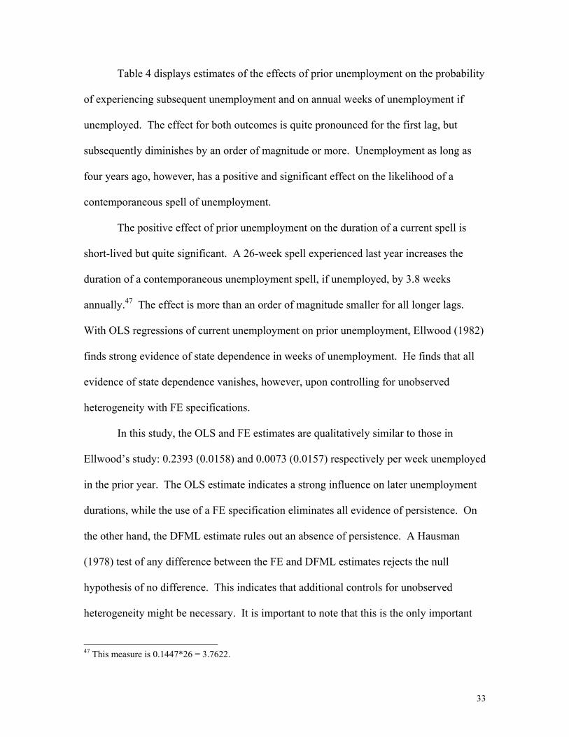
Table 4 displays estimates of the effects of prior unemployment on the probability
of experiencing subsequent unemployment and on annual weeks of unemployment if
unemployed. The effect for both outcomes is quite pronounced for the first lag, but
subsequently diminishes by an order of magnitude or more. Unemployment as long as
four years ago, however, has a positive and significant effect on the likelihood of a
contemporaneous spell of unemployment.
The positive effect of prior unemployment on the duration of a current spell is
short-lived but quite significant. A 26-week spell experienced last year increases the
duration of a contemporaneous unemployment spell, if unemployed, by 3.8 weeks
annually.47 The effect is more than an order of magnitude smaller for all longer lags.
With OLS regressions of current unemployment on prior unemployment, Ellwood (1982)
finds strong evidence of state dependence in weeks of unemployment. He finds that all
evidence of state dependence vanishes, however, upon controlling for unobserved
heterogeneity with FE specifications.
In this study, the OLS and FE estimates are qualitatively similar to those in
Ellwood’s study: 0.2393 (0.0158) and 0.0073 (0.0157) respectively per week unemployed
in the prior year. The OLS estimate indicates a strong influence on later unemployment
durations, while the use of a FE specification eliminates all evidence of persistence. On
the other hand, the DFML estimate rules out an absence of persistence. A Hausman
(1978) test of any difference between the FE and DFML estimates rejects the null
hypothesis of no difference. This indicates that additional controls for unobserved
heterogeneity might be necessary. It is important to note that this is the only important
47 This measure is 0.1447*26 = 3.7622.
33
instance where a DFML estimate appears substantively and statistically different from an
associated FE estimate. The FE estimator, however, cannot control well for possible
sample selection bias.
Long-Lived Blemishes
One of the most important measures of the long-term impact of youth
unemployment is the effect of a spell on future earnings. Forgone work experience may
reverberate throughout a young person’s life. Perhaps this is because one job leapfrogs
into another, and early unemployment would delay some of the first jumps. It may also
be because lost experience, as posited by dual labor market theorists, permanently tracks
young people into jobs characterized by low wages and little room for advancement.48
Ellwood (1982), for example, finds that prior work experience has a large and positive
earnings effect. Forgone experience, therefore, represents lost earnings power. This
observation is, in fact, the motivation for the theoretical model discussed earlier.
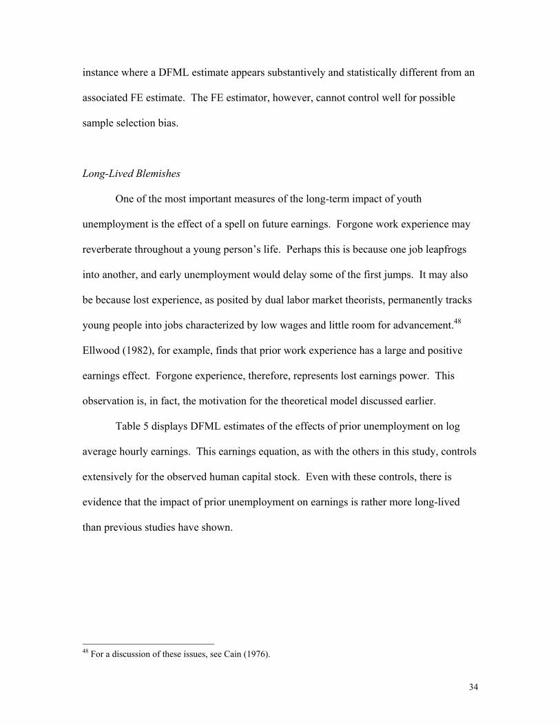
Table 5 displays DFML estimates of the effects of prior unemployment on log
average hourly earnings. This earnings equation, as with the others in this study, controls
extensively for the observed human capital stock. Even with these controls, there is
evidence that the impact of prior unemployment on earnings is rather more long-lived
than previous studies have shown.
48 For a discussion of these issues, see Cain (1976).
34

Table 5: Evidence of Long-Lived Blemishes in Wages (The Effect of One Week of Prior Unemployment on Log Average Hourly Earnings) Standard errors in parentheses Bold-faced indicates significance at the 5% level Method Lag of Annual Weeks of Unemployment
1 2 3 4 5
DFML
-0.0018 (0.0004)
-0.0013 (0.0004)
-0.0011 (0.0004)
-0.0008 (0.0004)
0.0002 (0.0004)
FE -0.0019 (0.0006)
-0.0019 (0.0006)
-0.0010 (0.0005)
-0.0012 (0.0005)
-0.0000 (0.0005)
OLS* -0.0023 (0.0008)
-0.0019 (0.0008)
-0.0014 (0.0007)
-0.0006 (0.0006)
0.0001 (0.0007)
* Robust standard errors.
The initial earnings effect of unemployment is large and quite precisely estimated.
The DFML estimates tend to be slightly smaller than those derived from FE or OLS
specifications, so we focus on them. A 26-week unemployment spell experienced last
year reduces wages by 4.7 percent.49 In terms of 2,000 hours worked at the average wage
rate in 1993, this is a reduction of over $1,543 in 2002 US dollars.50 A two standard error
lower bound amounts to a 2.6% reduction in hourly earnings or over $850. Further, a 26-
week spell experienced as long ago as three years reduces wages by 2.9 percent. To put
this magnitude into context, this reduction is equivalent to forgoing one-quarter to one-
half of a year of school.51 As predicted by the theoretical model, the earnings effect of
prior unemployment tapers off over time. Because it fully disappears after about four
years, the impact of unemployment on earnings is not permanent, as suggested by a scar
analogy. The magnitude and duration of this effect, however, make it much more than a
49 This measure is –0.0018*26 = –0.0468. 50 The average real wage rate in 1993 is 16.42 per hour in 2002 US dollars. At 2,000 hours, this yields average earnings of $32,840. 51 The impact (standard error) of an additional year of school on log wages is 0.0791 (0.0209) in the DFML model.
35

simple blemish. Unemployment experienced by a young man today will depress his
earnings for several years to come.
It is important to note that the negative earnings effect of prior unemployment
remains even after extensive controls for the observed and potentially endogenous human
capital stock. At first glance, this effect suggests that unemployment does not simply
represent forgone human capital, as suggested by dual labor market theorists. There is,
however, an alternative interpretation for the magnitude and duration of these effects on
earnings. The human capital variables used in this study are imperfect measures of
young men’s human capital stock. The “residual” earnings effect that we find could be
capturing these imperfectly measured human capital variables.
Simulating Unemployment’s Total Impact on Human Capital, Training, and Earnings
The above analysis of the earnings effect of prior unemployment above tells only
a partial story. A complete analysis would account simultaneously for the effects of
reduced human capital on earnings, as was implied by the theoretical model. For
example, if the theoretical model were correct and one could perfectly observe the human
capital stock, there should no independent effect of prior unemployment on earnings. A
complete evaluation of the impacts of unemployment must take into account the various
avenues through which it can affect later labor market outcomes. The DFML estimator,
since it models the entire early lifecycle of schooling, training, work, and unemployment,
provides a rich framework for tracing out the impacts of unemployment. In this section,
we use dynamic simulations with the DFML estimates to undertake such an analysis.52
52 The estimates presented in Tables 3 through 5 above were partial derivative effects. These simulations are more equivalent to total derivatives.
36

Before presenting the impacts of experiencing unemployment, it is necessary to
define precisely what is meant by “unemployment.” The literature on local average
treatment effects, Angrist, Imbens, and Rubin (1994) in particular, highlights the fact that
if individuals differ in their responses to a stimulus, there are usually an unlimited
number of possible average effects that one could calculate given continuous
instrumental or forcing variables. In this study we focus on two of these measures.53
The first measure we analyze is a population average effect. We define this as the
average impact in our sample on an outcome of interest if a worker were forced to
experience a six-month spell of unemployment at age 22.54 In practice, we start with all
individuals in our sample who were 14 to 16 years old in 1979, and we simulate
outcomes for them until age 21 using the complete set of DFML estimates. Then, for
each “individual” at age 22 who was not simulated to be in school or out of the labor
force, we “force” them to experience no unemployment at that age and complete their
simulated lifecycle for up to 10 additional years. We do this 50 times for each individual
and use this as a baseline simulation for individuals who were “forced” not to experience
unemployment. Next, starting at age 22, we force the same group of “individuals” to
experience 26 weeks of unemployment and a 50% reduction of their labor market
experience for that year. We also force a job change. Again, we complete the simulated
lifecycle for up to 10 additional years for this group. Our population average effect,
therefore, corresponds to those workers who, at age 22, were forced to experience 26
53 Heckman (1990) discusses alternative measures of the effect. 54 We do not use data from the “poor” white subsample in the NLSY in this study because of the peculiar selection issues that might arise. Appropriate weights for aggregating the stratified but random samples we use are not available. Consequently, we do not adjust our estimates to reflect the distribution of teenagers in the US at the time of the NLSY survey in 1979. The major consequence of this is that our sample greatly over-represents blacks and Hispanics.
37

weeks of unemployment. We refer to this effect as “Forced Unemployment” in the
graphs discussed below.
We also consider one particular form of the local average treatment effect. To do
this, we again examine each of the above “individuals” at age 22. At that age, we ask, for
individuals who were not in school and were working but did not experience any
unemployment, whether an increase of two standard deviations in the local
unemployment rate would induce them into unemployment.55 This defines a select group
of individuals who, because of their particular configuration of exogenous explanatory
variables up to age 22 and the configurations of their permanent and transitory
heterogeneity at age 22, were susceptible to becoming unemployed because of a
worsening local labor market. After selecting this group of individuals, as above we
“force” them to experience 26 weeks of unemployment, lose one half of their age-22 job
experience for that year, and experience a job change. Here, each individual’s “treatment
effect” is identical to the effect for them in the calculation of the population average
effect. In fact, the only difference between these two ways of measuring the effects of
unemployment is in the set of individuals used to define the “average” impact. The local
average effect captures the effect of unemployment on those most likely to be adversely
impacted by worsening economic conditions. We refer to this effect as “Induced
Unemployment” in the graphs discussed below.
Figure 3 displays simulation results for the impact of forced and induced
unemployment at age 22, described above, on job training behavior through age 31. The
55 A two standard deviation increase is 5.2 percentage points. For each “individual” we draw a complete set of all random numbers that would enter their simulations throughout these early lifecycle simulations and use the same set of random numbers under each of the two scenarios. This reduces the sampling variability of the estimated effects and is simple to do with pseudo random number generators.
38

top graphs display the level of training at each age and the lower graphs display the
change in the fraction of training at each age in response to the unemployment event.
The left hand graphs correspond to the population average effect and the right hand
graphs are for the local average treatment effect. The series with triangles on the level
graphs are for those who experienced unemployment at age 22. Later graphs follow the
same format. In the first two years after experiencing unemployment, there is a one- to
two-percentage point increase in the incidence of training (about a 10 to 20% increase)
for both unemployment effects. This is precisely the type of catch-up response suggested
by the theoretical model. At age 25 and later, however, there is a slightly lower tendency
for those who experienced unemployment at age 22 to train. While not displayed here,
examination of the simulation results for school attendance indicates a one- to three-
percentage point reduction in school attendance rates in the mid-twenties among those
who experienced unemployment at age 22. By age 30, however, there are no appreciable
differences in school attendance rates for either type of unemployment effect.
Figure 4 displays simulation results for the impact of forced and induced
unemployment at age 22 on employment rates through age 31. For both types of
“treatment” effects, there is evidence of long-lived persistence in the effect of
unemployment. From ages 25 to 31, employment rates for those who experienced
unemployment at age 22 are about two percentage points below the baseline rate. There
is some evidence that this persistence is shorter for those who were most likely to be
affected by worsening local labor market conditions. While not presented here, an
examination of the simulated hours of work (conditional on working) indicates a 75-hour
39
per year reduction in hours of work for those experiencing unemployment, with slightly
smaller impacts for the local average treatment.
Figure 5 presents simulation results for “state dependence” in unemployment.
Those who experienced unemployment at age 22 are at least 10 percentage points more
likely to experience unemployment at age 25, but by age 30 the difference in
unemployment rates becomes quite small. An examination of the simulated duration of
unemployment reveals about one to two additional weeks per unemployed person year at
age 23 for those who experienced unemployment at age 22. It falls to essentially zero
from age 24 to age 31. Again, the difference between the two types of unemployment
effects is relatively small.
Figure 6 contains simulation results for the impact of forced and induced
unemployment at age 22 on the log of average hourly earnings through age 31. After
experiencing unemployment at age 22, wages at age 23 are eight to nine percent below
their baseline level. According to the theoretical model, an immediate, and excessive,
decline in wages would be expected if individuals chose jobs with high levels of on-the-
job training after experiencing unemployment.56 Immediately after age 23, however, the
wage differential begins to shrink. The simple theoretical model also predicted this
effect. By age 27, the wage difference due to forced or induced unemployment falls to
about half its size at age 23. Nevertheless, wages for those who experienced forced or
induced unemployment at age 22 are still three to four percent lower by age 31. Again,
the difference between the two types of unemployment effects we consider is fairly small.
56 Informal training of this type might not be captured by our more formal measure of vocational training.
40

The simulation results presented here are generally consistent with the predictions
of the theoretical model.57 There is evidence of increased job training after experiencing
unemployment. Furthermore, wages appear to fall precipitously in the first year after
experiencing unemployment, which could reflect a combination of a relative loss in
human capital as well as an increase in the share of time that is spent training. This wage
gap rapidly diminishes, but remains substantial even nine years after either forced or
induced unemployment at age 22. This is precisely the pattern of wages one would
expect if there were real costs to unemployment at younger ages.
57 Unlike the somewhat small and relatively short-lived effects implied by the (partial-derivative) point estimates, however, these simulation results indicate fairly long-lived impacts of unemployment.
41

.075
.1.1
25.1
5.1
75.2
Inci
denc
e
21 22 23 24 25 26 27 28 29 30 31Age
Solid line is baseline simulationDashed line is unemployment simulation
Forced Unemployment
.075
.1.1
25.1
5.1
75.2
21 22 23 24 25 26 27 28 29 30 31Age
Solid line is baseline simulationDashed line is unemployment simulation
Induced Unemployment
Figure 3: Unemployment Impacts on Training
-.02
-.01
0.0
1.0
2Tr
aini
ng D
iffer
entia
l
21 22 23 24 25 26 27 28 29 30 31Age
Forced Unemployment
-.02
-.01
0.0
1.0
2
21 22 23 24 25 26 27 28 29 30 31Age
Induced Unemployment
42

.8.8
5.9
.95
1In
cide
nce
21 22 23 24 25 26 27 28 29 30 31Age
Solid line is baseline simulationDashed line is unemployment simulation
Forced Unemployment
.8.8
5.9
.95
1
21 22 23 24 25 26 27 28 29 30 31Age
Solid line is baseline simulationDashed line is unemployment simulation
Induced Unemployment
Figure 4: Unemployment Impacts on Employment
-.08
-.06
-.04
-.02
0Em
ploy
men
t Diff
eren
tial
21 22 23 24 25 26 27 28 29 30 31Age
Forced Unemployment
-.08
-.06
-.04
-.02
0
21 22 23 24 25 26 27 28 29 30 31Age
Induced Unemployment
43

0.2
5.5
.75
1In
cide
nce
21 22 23 24 25 26 27 28 29 30 31Age
Solid line is baseline simulationDashed line is unemployment simulation
Forced Unemployment
0.2
5.5
.75
1
21 22 23 24 25 26 27 28 29 30 31Age
Solid line is baseline simulationDashed line is unemployment simulation
Induced Unemployment
Figure 5: Unemployment Impacts on Subsequent Unemployment
0.1
.2.3
.4.5
.6.7
.8.9
1U
nem
ploy
men
t Diff
eren
tial
21 22 23 24 25 26 27 28 29 30 31Age
Forced Unemployment
0.1
.2.3
.4.5
.6.7
.8.9
1
21 22 23 24 25 26 27 28 29 30 31Age
Induced Unemployment
44
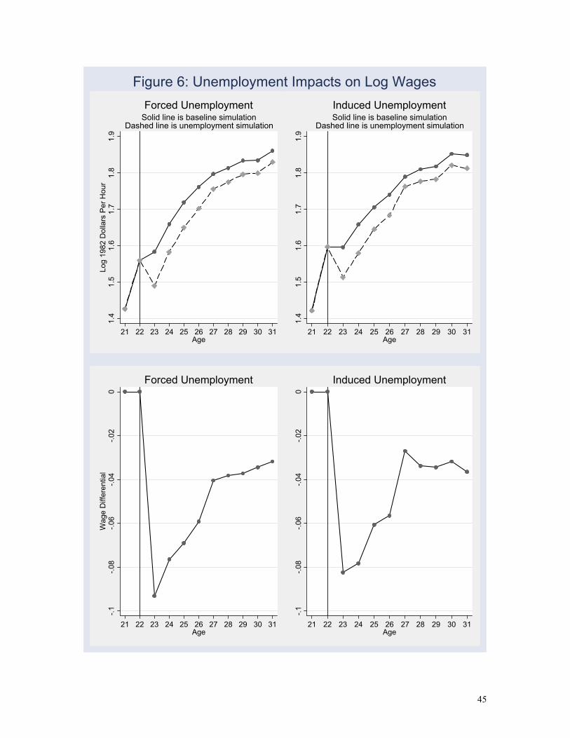
1.4
1.5
1.6
1.7
1.8
1.9
Log
1982
Dol
lars
Per
Hou
r
21 22 23 24 25 26 27 28 29 30 31Age
Solid line is baseline simulationDashed line is unemployment simulation
Forced Unemployment
1.4
1.5
1.6
1.7
1.8
1.9
21 22 23 24 25 26 27 28 29 30 31Age
Solid line is baseline simulationDashed line is unemployment simulation
Induced Unemployment
Figure 6: Unemployment Impacts on Log Wages
-.1-.0
8-.0
6-.0
4-.0
20
Wag
e D
iffer
entia
l
21 22 23 24 25 26 27 28 29 30 31Age
Forced Unemployment
-.1-.0
8-.0
6-.0
4-.0
20
21 22 23 24 25 26 27 28 29 30 31Age
Induced Unemployment
45

VI. CONCLUSIONS
This research provides several new insights to our understanding of the youth
labor market and, in particular, the long-term impacts of youth unemployment on later
labor market outcomes. Most importantly, there is strong evidence of a catch-up
response to unemployment. That is, an unemployment spell experienced today increases
the likelihood that a young person trains in the near future. A dynamic model of human
capital accumulation predicts this catch-up response. Both this theoretical implication as
well as empirical evidence of it is new to the literature. Of course, we have made several
simplifying assumptions to reach both the theoretical predictions and the empirical
conclusions.
We also uncover relatively large longer-term impacts on earnings from
unemployment experienced early in the employment lifecycle. A 26-week spell of
unemployment experienced at age 22 results in persistently lower wages through the end
of our simulations at age 31. The immediate wage impact is quite large and is consistent
with a catch-up response in which workers pay for informal on-the-job training by
accepting lower wages. Nevertheless, substantial wage differentials remain after many
years. Based on our simulation results, when evaluated at 2,000 hours per year and in
2002 US dollars, a 26-week unemployment spell experienced at age 22 results in an
earnings loss of $1,400 to $1,650 at age 26 and in a loss of $1,050 to $1,150 at age 30.
These lasting impacts of unemployment experienced at younger ages suggest that youth
unemployment may not be a purely transitory phenomenon.
46

APPENDIX 1: A CONCEPTUAL FRAMEWORK
Notation and Setup:
Define time to be discrete and finite, t=1, 2, 3, …, T.
Define P to be the probability of being unemployed in any particular time period t, where
0 ≤ P < 1.
Define st to be the fraction of each working period devoted to (planned) training, where 0
≤ st ≤1.
Define λ to be the fraction of the year an individual is not unemployed, where 0 ≤ λ ≤1.
Define Ht to be the human capital stock (or productivity) of an individual at period t.
Define w to be the rental rate for human capital, which is constant over time.
Define β to be the rate at which individuals discount future incomes.
Define f(st) to be the production function of new human capital. We assume that
f '(.) > 0, f ''(.) < 0, and that the production function satisfies the Inada conditions (Inada,
1964).58 These conditions imply that the marginal product of training is large when an
individual does at least a little training, and, therefore, given the possibility of training, it
is always optimal to devote some fraction of time to training.
Human capital evolves as Ht+1 = Ht + f(st).
We assume that all training takes place on the job and that the fraction of time
devoted to training is determined before an individual learns whether he is to become
unemployed. If he does not experience unemployment, his potential income at time t is
wHt and his disposable income is potential income minus the opportunity cost of training,
w(1- st)Ht. On the other hand, if he becomes unemployed, then potential and disposable
58 Given the finite time horizon, we in fact only rely on the condition that limk→0 f'(k) = ∞.
47

incomes are given by λwHt and λw(1- st) Ht, respectively. We assume the fraction of
time that is spent unemployed, if unemployment is experienced, is not stochastic.
Period T
At the last time period, it is never optimal to train because there is no future return to
training. In this case,
wHT if the individual works full-time.
Disposable Income = λwHT if the individual is unemployed.
We focus on the situation in which an individual maximizes the present
discounted value of his disposable income. Therefore, the individual’s expected utility as
a function of the human capital stock at the start of the final period T is
EVT (HT) = (1 – P)(wHT) + P(λwHT) .
Period T–1:
In period T–1, an individual makes a decision about how much time to devote to
training. Time spent training is not paid, but training in period T–1 increases the amount
of human capital in period T. This in turn increases disposable income in the last period.
According to our formulation of the model, training is possible only when employed.
Therefore, at the beginning of period T-1 an individual faces the following optimization
problem:
max (H1−TEV T-1) = ST-1
P{βT-1λ (1–ST-1) wHT-1 + βTVT (HT-1 + f (λST-1))} + (1-P){βT-1 (1–ST-1) wHT-1 + βTVT(HT-1 + f (ST-1))}
This optimization can be rewritten as:
48

max (H1−TEV T-1) = ST-1
= P{βT-1λ (1–ST-1) wHT-1 + βTPλw (HT-1 + f (λST-1)) + βT(1-P)w(HT-1 + f(λST-1))} +
(1-P){βT-1 (1–ST-1) wHT-1 + βTPλw (HT-1 + f (ST-1)) + βT(1-P)w(HT-1 + f(ST-1))}
The first order condition (FOC) for the optimal choice of the fraction of time to devote to
training is given by:
=∂
∂
−
−−
1
11 )(
T
TT
SHV - βT-1PλwHT-1 + βTP2λ2wf '(λST-1) + βTP(1–P)λw f '(λST-1)
- βT-1(1–P)wHT-1 + βTP(1–P)λw f '(ST-1) + βT(1–P)2w f '(ST-1)
= 0
The second order condition (SOC) for a maximum is satisfied because of the concavity of
the human capital production function:
=∂∂
−
−2
1
12
T
T
SV βTP2λ3wf"(λST-1) + βT P(1–P)λ2wf"(λST-1) +
βTP(1–P)λwf''(ST-1) + βT(1–P)2wf "(ST-1) < 0
These conditions ensure that there exists a unique level of training that maximizes
an individual's objective function at time period T-1. After re-arrangement, the decision-
rule for optimal training at T-1, given the amount of capital accumulated prior to this
period, is:
β [Pλw + (1-P)w] [f '(λST-1)Pλ + f '(ST-1)(1-P)] = [Pλw + (1-P)w] HT-1
or
wHT-1 =β w[f '(λST-1)Pλ + f '(ST-1)(1-P)]
49

The economic interpretation of this condition is that the expected income loss
from additional training today should be equal to the expected present discounted value
of the gain from the addition human capital available in the next time period.
Let S be the optimal choice of training as a function of the level of the
human capital stock at the beginning of period T-1. By the Implicit Function Theorem
(IFT):
)( 1*
1 −− TT H
02
1*
12
11*
12
1
1*
<
∂∂
∂∂∂
−=
−
−
−−
−
−
−
T
T
TTT
T
T
SV
HSV
dHdS
because
=∂∂
∂
−−
−
11*
12
TT
T
HSV
- βT-1 Pλw - βT-1(1-P)w < 0
and
0* 2
1
12
<∂∂
−
−
T
T
SV from the second order condition.
Therefore, those entering period T-1 with lower human capital stocks will train
more than those entering the period with higher human capital stocks. In anticipation of
the main theoretical result, suppose there were two identical individuals at the start of
period T-2, and one experienced unemployment while the other did not. Upon entering
period T-1, the individual who experienced unemployment in T-2 would choose to train
more during period T-1 than the individual who did not experience unemployment.
It is important to note that we have a single value function at the start of this time
period, which can be evaluated at different levels of the human capital stock. It is useful
to rewrite the value function in a general form and prove its concavity in HT-1.
50

VT-1(S*T-1(HT-1), HT-1) =
P{βT-1λ(1-ST-1)wHT-1 + βTPλw[HT-1 + f(λST-1)] + βT(1-P)w[HT-1 + f(λST-1)]} +
(1-P){βT-1(1-ST-1)wHT-1 + βTPλw[HT-1 + f(ST-1)] + βT(1-P)w[HT-1 + f(ST-1)]}
By the Envelope Theorem the first total derivative of this value function is:
1
1
1
1
1
1*
1*
1
1
111*
1 )),((
−
−
−
−
−
−
−
−
−
−−−−
∂∂
=∂∂
+∂∂
=T
T
T
T
T
T
T
T
T
TTTt
HV
HV
dHdS
SV
dHHHSdV
since 01
*1 =
∂∂
−
−
T
T
SV by the FOCs for a maximum.
Then
=∂∂
−
−
1
1
T
T
HV βT-1Pλw(1-S*
T-1) + βTP2λw + βTP(1-P)w + βT-1(1-P)w(1-S*T-1) + βTP(1-P)λw +
βT(1-P)2w = positive constant.
By the Envelope Theorem the second total derivative is:
0)),((2
1
1*
21
*1
2
1
12
21
1*2
1*
1
2
1_
1*
21
*1
2
21
111*
12
<
∂∂
=∂∂
+∂∂
+
∂∂
=−
−
−
−
−
−
−
−
−
−−
−
−
−
−−−−
T
T
T
T
T
T
T
T
T
T
T
T
T
T
T
TTTT
dHdS
SV
HV
dHSd
SV
dHdS
SV
dHHHSVd
because 01
*1 =
∂∂
−
−
T
T
SV by FOC,
021
12
=∂∂
−
−
T
T
HV because
1
1
−
−
∂ T
T
HV∂ = positive constant, and
021
*1
2
<∂∂
−
−
T
T
SV by SOCs of optimization problem at period T-1.
The concavity of the value function in time period T-1 is sufficient to ensure that the
FOCs at time T-2 define behaviors necessary to maximize the objective function at T-2.
51

Period T-2:
The individual’s optimization problem in T-2:
max EVT-2(HT-2) = P {βT-2λ(1-ST-2)wHT-2 + βT-1VT-1(HT-2 + f(λST-2))} ST-2
+ (1-P) {βT-2(1-ST-2)wHT-2 + βT-1VT-1(HT-2 + f(ST-2))}, where
VT-1(HT-2 + f(λST-2)) = = P βT-1λ(1-ST-1)w[HT-2 + f(λST-2)] +
+ βTPλw[HT-2 + f(λST-2) + f(λST-1)] + βT(1-P)w[HT-2 + f(λST-2) + f(λST-1)]
+ (1-P) βT-1(1-ST-1)w[HT-2 + f(λST-2)] +
+βTPλw[HT-2 + f(λST-2) + f(ST-1)] + βT(1-P)w[HT-2 + f(λST-2) + f(ST-1)]
and
VT-1(HT-2 + f(ST-2)) = = P βT-1λ(1-ST-1)w[HT-2 + f(ST-2)] +
+ βTPλw[HT-2 + f(ST-2) + f(λST-1)] + βT(1-P)w[HT-2 + f(ST-2) + f(λST-1)]
+ (1-P) βT-1(1-ST-1)w[HT-2 + f(ST-2)] +
+βTPλw[HT-2 + f(ST-2) + f(ST-1)] + βT(1-P)w[HT-2 + f(ST-2) + f(ST-1)]
The value function in T-2 is concave when both VT-1(HT-2 + f(λST-2)) and
VT-1(HT-2 + f(ST-2)) are concave in human capital stock, a result which was proved above
for arbitrary levels of the human capital stock at the start of T-1.
Conclusions for T, T-1, and T-2:
1. V'T (.) = positive constant and V"T (.) = 0 because the value function in the last
period T is linear in human capital/income.
52

2. V'T-1 (.) > 0 and V"T-1 (.) < 0 because the value function of period T-1 is concave
in the human capital stock (or income).
3. V'T-2 (.) > 0 and V"T-2 (.) < 0 because the value function of period T-2 is concave
in human capital as it is a linear combination of a linear utility function and a
concave value function in period T-1.
Periods t < T:
The individual’s optimization problem in each earlier period t is given by:
max EVt(Ht) = P{βtλ(1 – St)wHt + βt+1Vt+1(Ht + f(λSt))} + St
(1–P){βt(1–St)wHt + βt+1Vt+1(Ht + f(St))}
FOC:
;0)('))((')1()1(
)('))((')(
11
11
=+−+−−
++−=∂
∂
++
++
ttttt
tt
ttttt
tt
t
tt
SfSfHVPwHP
SfSfHVPwHPSHV
ββ
λλλβλβ
After rearrangement, the FOC for optimal training in an arbitrary period t is:
[ ][ ] t
tttttttt
HwPwPPSfSfHVPSfSfHV
)1()1)(('))((')('))((' 11
−+=−+++ ++
λλλλβ
Now we prove that the value function of an arbitrary period t < T is concave in
human capital stock (or income). To do this, we show that concavity of the value
function in the next period guarantees concavity in any arbitrary period t < T.
By the Envelope Theorem, the first total derivative of the value function in period
t is:
.)),(()),(()),(()),(( ***
*
**
t
tttt
t
tttt
t
t
t
tttt
t
tttt
HHHSV
HHHSV
dHdS
SHHSV
dHHHSdV
∂∂
=∂
∂+
∂∂
=
53

Now,
[ ][ ]))((')1()1(
))(('')1()),((
*1
1*
*1
1**
tttt
tt
tttt
tt
t
tttt
SfHVwSP
SfHVwSPH
HHSV
++−−+
++−=∂
∂
++
++
ββ
λβλβ
Since V is true for time period T-3, it holds by induction for all earlier time
periods and the value function is everywhere an increasing function of the human capital
stock.
0(.)' 1 >+t
By the Envelope Theorem, the second total derivative is:
0)),(( 22*
2*
22
2
*2
*
2*
2*
2
2
*2
<∂∂
+
∂∂
=∂∂
+∂∂
+
∂∂
=t
t
t
tt
t
t
t
t
t
t
t
t
t
t
t
t
t
tttt
HV
dHdS
SV
HV
dHSd
SV
dHdS
SV
dHHHSVd
where
0* =∂∂
t
t
SV (by FOC);
0))(()1())(( *1
"1*1
"12
2
<+−++=∂∂
++
++
tttt
tttt
t
t SfHVPSfHVPHV βλβ
provided that the value function of the next period is concave in the stock of human
capital. Again, this condition holds for T-3 and, by induction, for all earlier time periods.
The period t second order condition for the maximal choice of training intensity is
given by:
( )
( ) )(''))((')1()('))(('')1(
)(''))((')('))(('')(
112
11
21
121
12
2
ttttt
ttttt
ttttt
ttttt
t
tt
SfSfHVPSfSfHVP
SfSfHVPSfSfHVPS
HV
+−++−+
++++=∂
∂
++
++
++
++
ββ
λλλβλλλβ
The concavity of the value function of human capital in the next period t+1, the
positive first derivative of this value function, and the concavity of the human capital
54

production function guarantee the concavity of the value function at an arbitrary period.
This concavity, in turn, ensures that the first order conditions describe the behaviors
necessary to maximize the expected present discounted value of disposable earnings at
each point in time.
Next, we establish that a larger stock of human capital results in lower investment
in additional human capital at each point in time. Since
0)('))(('')1()1(
)('))((''
11
11
2
<+−+−−
++−=∂∂
∂
++
++
tttttt
tttttt
tt
t
SfSfHVPWP
SfSfHVPWPHS
V
ββ
λλλβλβ
because of the concavity of the value function in t+1 and human capital production
function. Therefore, by the Implicit Function Theorem:
0)()(
2*
2
*
2
*
<−−
−=
∂∂
∂∂∂
−=
t
t
ttt
t
t
SV
HSV
dHdS for any arbitrary period t < T.
The result derived for period T-1 with an explicit formulation of the utility and
value functions holds for an arbitrary period as well. Therefore, an individual's optimal
behavior is to invest less in training at higher levels of human capital holding age, t,
constant. Since an “exogenous” unemployment shock reduces the human capital stock at
the start of the next time period, those who experienced unemployment will choose to
undertake more training in the next time period. This establishes Proposition 1 in the
main text.
To establish Proposition 2 in the text, suppose that, at the start of period t+1, two
otherwise identical individuals have human capital stocks that differ by an arbitrary
amount ∆. This difference in human capital stocks could have arisen because these two
55

individuals had different unemployment experiences during period t. At the start of t+1,
their potential earnings would differ by w∆. By Proposition 1, the individual with the
lower human capital stock in t will choose to invest more in additional human capital at
t+1. Let and be these two optimal decisions, where and the superscripts
N and U stand, respectively, for not having been unemployed at t and having been
unemployed at time period t. At the start of period t+2, if neither individual experienced
unemployment during t+1, then the potential earnings would differ by
Nts 1+
Uts 1+
Ut
Nt ss 11 ++ <
[ ]( ) ∆<−+∆ wffw )) +sUt( 1+s N
t( 1 because higher levels of training increase the stock of
human capital. If both individuals had experienced unemployment during t+1, then
potential earnings at the start of t+2 would differ by [ ]( ) ∆<+∆ + wsfw Ut )( 1λ−+sf N
t )( 1λ ,
which also is a convergence of the potential human capital stocks. So, provided that
unemployment experiences do not increase the propensity to experience future
unemployment too severely (the model assumes a zero effect), there will be a
convergence in expected potential earnings from t+1 to t+2. By induction, there will be
continued convergence in expected earnings for t+3 and for later periods.
The first part of Proposition 3 in the text follows directly because the fraction of
time spent earning income (i.e., not spent training) is higher for those who did not
experience unemployment at time t. Therefore, the observed disposable earnings
differential at t+1 is larger than that that implied if there were no training differential in
response to experiencing unemployment at t. In particular,
∆+−>+−++∆+−=+−−∆++−
wUts
tHwUtsN
tswUtstHwU
tstHwNts
)11(
)()11()11()()11()()11(
56

The second part of Proposition 3 in the text follows from two observations. First,
for a given human capital differential between two individuals, there will be a larger
training differential at t+1 than at t+2 because the future benefit of additional human
capital declines as t approaches T, holding constant one of the individual’s human capital
stock. The second observation follows form the concavity of the human capital
production function. Consider holding constant the human capital at t+2 for the
individual with the higher level of human capital at the start of period t+1 by examining a
particular type of (un)employment experience during t+1. Following from the optimal
catch-up response in Proposition 1, at higher levels of the other individual’s human
capital stock for the same type of t+1 (un)employment experience, the differentials in the
training responses at t+2 will be smaller than otherwise in the absence of the immediate
catch-up response. Because of the model’s assumption that future unemployment
propensities do not depend on previous unemployment events, this implies that we can
use equal “weights” for the two individuals when integrating over possible subsequent
unemployment experiences.
These two observations, in conjunction, imply that the subsequent average
training intensities for the two types of individuals, defined by of one type experiencing
unemployment at period t, will become more similar over time. Therefore, the
convergence of their disposable earnings over time will reflect not only the convergence
in their human capital stocks but also the convergence in the optimal share of time that is
spent training. The observed convergence in their disposable earnings after time t+1,
therefore, would happen at a faster rate than would be implied by solely the convergence
in their human capital stocks.
57

Model Limitations
This model is a simple but useful tool. It directly links the present and the future
through the process of human capital investment and accumulation. By establishing
equivalence between an involuntary unemployment spell and an exogenously constrained
human capital stock, it can examine the spell’s effects on future behavior and outcomes.
The duration of unemployment spells, however, will vary by the intensity and duration of
job search. While the duration of search is potentially observable, intensity is not.
Search intensity is a component of the unobserved heterogeneity that makes
unemployment a potentially endogenous variable in statistical analyses. It is unclear,
however, what search theory would contribute to this simple framework in particular.
The inverse relationship between search intensity and duration is unlikely to yield
unambiguous theoretical predictions. In this case, the answers to the questions posed
here are entirely empirical. On the other, this simple model uses a standard human
capital framework to analyze these issues. Most labor economists probably accept that
one mechanism through which current unemployment can affect future behavior is the
human capital stock. Notwithstanding this acceptance, a model like this has not been
found in the youth labor market literature. Further, even if all youth unemployment is
simply time spent watching television, it may still be relevant to ask whether there are
long-term consequences, especially for future earnings.
Finally, the model is expressed in terms of involuntary unemployment. We note
that much of the literature on job search views the distinction between quits and layoffs
to have little economic content. See, for example, McLaughlin (1991). As is trenchantly
noted by Gottshalk and Maloney (1985), however, much of this debate is tautological.
58

To summarize their argument, even coerced decisions can be viewed as voluntary since
they result from re-optimization under an alternate set of constraints. In this case, all
unemployment may be considered voluntary. It is not possible to distinguish the nature
of unemployment using NLSY79 data. Total unemployment, however, is identically the
sum of its involuntary and voluntary components. Isolating one of these components is
sufficient to distinguish them empirically, since the other is identically the residual.
Local variation in labor market conditions over time and exogenous changes in mandated
minimum wages over time are potentially suitable instruments to make this empirical
distinction.
59

APPENDIX 2: MAXIMUM LIKELIHOOD DISCRETE FACTOR ESTIMATES Log-likelihood function value: -220859.39 Number of parameters: 444 COEFF. STD.ERR T-RATIO Any Schooling (as): 1 cons_sch -5.40282 2.30871 -2.34019 2 year 0.05649 0.01169 4.83332 3 afqt 0.00741 0.00056 13.15392 4 readmat -0.03012 0.03315 -0.90864 5 libcard 0.06536 0.02585 2.52829 6 livpar 0.06613 0.02518 2.62634 7 prot -0.02088 0.02485 -0.84026 8 black 0.16552 0.03096 5.34641 9 hisp 0.04341 0.03396 1.27802 10 nc 0.07289 0.04575 1.59320 11 so -0.00419 0.06025 -0.06959 12 we 0.04072 0.05643 0.72156 13 urb 0.03687 0.03246 1.13591 14 ur 0.00670 0.00433 1.54613 15 mw 0.79964 0.48936 1.63403 16 mwage -0.15555 0.02050 -7.58685 17 mwhgc 0.24087 0.02147 11.22086 18 ugtuit -0.12351 0.25891 -0.47706 19 expsec -0.26184 0.20309 -1.28928 20 expps -0.21402 0.11324 -1.88995 21 age 0.04831 0.11669 0.41398 22 age2 0.00673 0.00163 4.13370 23 exp -0.17608 0.01167 -15.08939 24 exp2 0.00670 0.00057 11.69062 25 hgc -0.42516 0.06735 -6.31241 26 dum12y -0.57403 0.04710 -12.18772 27 coldeg -1.07555 0.05241 -20.52079 28 lag1sc 1.58061 0.03599 43.91313 29 lag1wu -0.00688 0.00143 -4.80965 30 lag2wu -0.00688 0.00151 -4.54923 31 lag3wu -0.00456 0.00171 -2.66375 32 lag4wu -0.00432 0.00180 -2.39687 33 lag5wu 0.00064 0.00178 0.36010 34 cumtr 0.02549 0.01142 2.23258 35 year79 -0.31345 0.10275 -3.05065 36 year8082 -0.08663 0.06421 -1.34918 37 year9294 -0.11862 0.06743 -1.75917 38 age1415 0.94031 0.24527 3.83375 39 age16 1.15128 0.19533 5.89391 40 age17 0.53692 0.15164 3.54075
60

41 age1819 -0.11913 0.09632 -1.23677 42 age2021 -0.36704 0.06483 -5.66170 43 rhod11 -0.12899 0.08088 -1.59496 44 rhod12 -0.16098 0.06922 -2.32545 Any Training (tr): 45 cons_tra -7.62289 1.86784 -4.08113 46 year 0.01437 0.01215 1.18265 47 afqt 0.00109 0.00051 2.13251 48 readmat 0.01565 0.03109 0.50341 49 libcard 0.04166 0.02390 1.74324 50 livpar -0.01075 0.02421 -0.44401 51 prot 0.01949 0.02231 0.87363 52 black -0.00854 0.03073 -0.27794 53 hisp 0.02800 0.03277 0.85448 54 nc 0.13633 0.03974 3.43093 55 so 0.04304 0.05299 0.81225 56 we 0.08520 0.05038 1.69113 57 urb -0.01042 0.02599 -0.40090 58 ur -0.00846 0.00372 -2.27217 59 mw 0.76114 0.37831 2.01196 60 mwage -0.00273 0.01451 -0.18787 61 mwhgc -0.05418 0.01885 -2.87400 62 ugtuit -0.32935 0.22278 -1.47837 63 expsec 0.35550 0.16719 2.12634 64 expps -0.26458 0.09504 -2.78380 65 age 0.18231 0.07622 2.39182 66 age2 -0.00391 0.00085 -4.59464 67 exp 0.02128 0.01014 2.09937 68 exp2 -0.00004 0.00044 -0.09536 69 hgc 0.20305 0.05946 3.41472 70 dum12y 0.11290 0.03762 3.00108 71 coldeg 0.15048 0.04559 3.30105 72 lag1wu 0.00351 0.00134 2.61187 73 lag2wu 0.00111 0.00154 0.72009 74 lag3wu -0.00188 0.00159 -1.18583 75 lag4wu 0.00061 0.00158 0.38600 76 lag5wu -0.00054 0.00165 -0.32558 77 cumtr 0.25118 0.00930 27.02045 78 year79 -0.27332 0.09459 -2.88957 79 year8082 0.16708 0.05659 2.95256 80 year9294 -0.10617 0.04705 -2.25641 81 oldcoh -0.01503 0.03663 -0.41017 82 lag1ch 0.03625 0.05080 0.71350 83 lag2ch 0.01289 0.05598 0.23032 84 lag3ch -0.11927 0.06042 -1.97416 85 lag4ch -0.00804 0.06231 -0.12911
61

86 lag5ch -0.12287 0.06438 -1.90856 87 rhod21 0.16462 0.07470 2.20368 88 rhod22 0.08093 0.05749 1.40782 Any Work (work): 89 cons_wo 22.32405 5.19979 4.29326 90 year -0.12317 0.03333 -3.69558 91 afqt 0.00389 0.00155 2.51672 92 readmat -0.10216 0.06703 -1.52404 93 libcard -0.09337 0.05690 -1.64089 94 livpar 0.06955 0.05639 1.23347 95 prot -0.02522 0.05907 -0.42704 96 black -0.42809 0.07549 -5.67083 97 hisp -0.20362 0.08292 -2.45555 98 nc 0.34945 0.10242 3.41181 99 so 0.44976 0.13748 3.27137 100 we 0.27055 0.12232 2.21181 101 urb -0.03057 0.07020 -0.43552 102 ur -0.04419 0.00861 -5.13382 103 mw -3.77947 1.07507 -3.51554 104 mwage 0.11122 0.04210 2.64217 105 mwhgc 0.10043 0.04463 2.25040 106 ugtuit 0.51153 0.57046 0.89670 107 expsec 1.11080 0.41570 2.67213 108 expps -0.02553 0.28613 -0.08921 109 age -0.06406 0.20003 -0.32028 110 age2 -0.00832 0.00206 -4.03865 111 exp 0.54387 0.02508 21.68812 112 exp2 -0.01910 0.00172 -11.09092 113 hgc -0.20883 0.14067 -1.48456 114 dum12y 0.03572 0.08737 0.40881 115 coldeg 0.58514 0.22084 2.64967 116 lag1wu -0.00144 0.00233 -0.62084 117 lag2wu 0.00259 0.00292 0.88722 118 lag3wu 0.00877 0.00317 2.76588 119 lag4wu 0.00004 0.00310 0.01310 120 lag5wu 0.00379 0.00269 1.41008 121 cumtr 0.15554 0.03191 4.87432 122 year79 -0.24914 0.27897 -0.89308 123 year8082 0.14971 0.14845 1.00847 124 year9294 0.20260 0.12490 1.62207 125 oldcoh 0.04065 0.10252 0.39653 126 lag1ch -0.37553 0.07427 -5.05657 127 lag2ch -0.07009 0.08997 -0.77907 128 lag3ch -0.16504 0.09275 -1.77949 129 lag4ch -0.01650 0.09935 -0.16612 130 lag5ch -0.00535 0.10855 -0.04926
62

131 rhod31 -3.78445 0.23214 -16.30238 132 rhod32 -0.24393 0.12996 -1.87694 Any Unemployment(un): 133 cons_un -0.74671 4.69515 -0.15904 134 year 0.06530 0.02525 2.58576 135 afqt -0.00604 0.00101 -5.98804 136 readmat -0.04357 0.05226 -0.83374 137 libcard -0.00557 0.04256 -0.13093 138 livpar -0.04730 0.04267 -1.10830 139 prot 0.05083 0.04439 1.14523 140 black 0.18790 0.05589 3.36207 141 hisp -0.00868 0.06349 -0.13677 142 nc 0.29733 0.08151 3.64801 143 so 0.27573 0.10801 2.55272 144 we 0.32793 0.10133 3.23614 145 urb 0.08488 0.05182 1.63807 146 ur 0.06484 0.00735 8.81730 147 mw 0.35621 1.06182 0.33547 148 mwage -0.02910 0.04007 -0.72628 149 mwhgc 0.04306 0.04101 1.04981 150 ugtuit 0.08569 0.42106 0.20352 151 expsec 1.28847 0.34161 3.77172 152 expps 0.38318 0.18632 2.05657 153 age -0.38773 0.19468 -1.99156 154 age2 0.00726 0.00212 3.42409 155 exp 0.00083 0.02038 0.04049 156 exp2 -0.00013 0.00115 -0.11505 157 hgc -0.20773 0.12884 -1.61228 158 dum12y -0.09233 0.07082 -1.30378 159 coldeg 0.01134 0.11492 0.09868 160 lag1wu 0.09265 0.00386 23.98149 161 lag2wu 0.00411 0.00281 1.46375 162 lag3wu 0.00688 0.00274 2.51465 163 lag4wu 0.00851 0.00279 3.05033 164 lag5wu 0.00302 0.00252 1.19717 165 cumtr -0.05241 0.01995 -2.62756 166 year79 0.12579 0.31275 0.40221 167 year8082 0.46921 0.14090 3.33015 168 year9294 -0.17808 0.09167 -1.94250 169 oldcoh 0.10904 0.07092 1.53750 170 lag1ch 0.30694 0.08554 3.58822 171 lag2ch 0.22186 0.08693 2.55207 172 lag3ch 0.12513 0.08415 1.48708 173 lag4ch 0.22416 0.09049 2.47731 174 lag5ch 0.00448 0.08995 0.04984 175 rhod41 1.87575 0.14864 12.61938
63

176 rhod42 -1.36867 0.10659 -12.84061 Any Job Change (ch): 177 cons_ch 4.39813 5.19413 0.84675 178 year -0.00547 0.03051 -0.17931 179 afqt -0.00460 0.00128 -3.58572 180 readmat -0.03884 0.06086 -0.63824 181 libcard 0.02831 0.05195 0.54486 182 livpar -0.06131 0.05110 -1.19976 183 prot 0.05564 0.05487 1.01414 184 black 0.19311 0.06956 2.77607 185 hisp 0.04618 0.07570 0.61012 186 nc 0.08828 0.10065 0.87706 187 so 0.03647 0.13019 0.28009 188 we 0.13910 0.11870 1.17189 189 urb 0.06088 0.06629 0.91851 190 ur 0.04999 0.00893 5.59698 191 mw -0.15158 1.06520 -0.14231 192 mwage -0.00485 0.03991 -0.12158 193 mwhgc 0.03470 0.04340 0.79968 194 ugtuit -0.36683 0.54402 -0.67430 195 expsec 0.44405 0.41192 1.07800 196 expps -0.28266 0.22398 -1.26197 197 age -0.33359 0.20315 -1.64209 198 age2 0.00643 0.00223 2.89025 199 exp 0.00292 0.02412 0.12115 200 exp2 -0.00092 0.00124 -0.74296 201 hgc -0.16177 0.13824 -1.17021 202 dum12y -0.09284 0.08463 -1.09706 203 coldeg 0.05012 0.14111 0.35518 204 lag1wu 0.01654 0.00236 7.01810 205 lag2wu 0.00645 0.00245 2.63323 206 lag3wu -0.00361 0.00247 -1.46429 207 lag4wu 0.00527 0.00267 1.97501 208 lag5wu 0.00010 0.00248 0.04087 209 cumtr -0.01271 0.02598 -0.48897 210 year79 -1.87776 0.28855 -6.50768 211 year8082 0.04009 0.13133 0.30531 212 year9294 -0.12556 0.10816 -1.16090 213 oldcoh -0.06027 0.09013 -0.66868 214 lag1ch 0.17112 0.07020 2.43763 215 lag2ch 0.10180 0.08085 1.25909 216 lag3ch 0.25839 0.07755 3.33208 217 lag4ch 0.24215 0.08722 2.77629 218 lag5ch 0.17742 0.09300 1.90765 219 rhod51 1.77302 0.18589 9.53822 220 rhod52 -0.98839 0.12069 -8.18933
64

Annual Hours Work (h, Conditional on Working): 221 cons_hw 3732.28816 959.17900 3.89113 222 year -17.08248 7.64238 -2.23523 223 afqt 0.91746 0.31697 2.89449 224 readmat -17.59887 17.79130 -0.98918 225 libcard -9.01697 14.17603 -0.63607 226 livpar 49.54895 15.13751 3.27326 227 prot -1.21263 13.91489 -0.08715 228 black -94.30124 18.05057 -5.22428 229 hisp -31.05630 19.69059 -1.57722 230 nc -32.60257 22.34989 -1.45873 231 so 18.17003 27.16728 0.66882 232 we -10.92480 25.86992 -0.42230 233 urb -51.91571 13.25442 -3.91686 234 ur -17.19556 1.63393 -10.52406 235 mw -163.06607 192.18122 -0.84850 236 mwage -1.58275 7.32497 -0.21608 237 mwhgc 13.85266 7.48268 1.85130 238 ugtuit 322.02056 102.98940 3.12673 239 expsec -59.09172 78.00897 -0.75750 240 expps -39.11304 45.31896 -0.86306 241 age 54.30585 35.77315 1.51806 242 age2 -1.81219 0.37444 -4.83976 243 exp 112.38616 4.71022 23.86007 244 exp2 -2.60099 0.17962 -14.48028 245 hgc 11.62469 23.61971 0.49216 246 dum12y -12.82351 20.41242 -0.62822 247 coldeg 56.21566 32.23167 1.74411 248 lag1wu -6.13522 0.55146 -11.12538 249 lag2wu 1.48764 0.56054 2.65397 250 lag3wu 1.30891 0.55155 2.37315 251 lag4wu 1.39288 0.55675 2.50183 252 lag5wu 1.24083 0.53497 2.31943 253 cumtr 25.07666 4.79220 5.23280 254 year79 -80.94356 51.77019 -1.56352 255 year8082 -110.73201 24.69076 -4.48475 256 year9294 54.12616 19.64162 2.75569 257 oldcoh 44.50441 23.64567 1.88214 258 lag1ch -115.63616 16.58982 -6.97031 259 lag2ch -34.60553 16.23511 -2.13152 260 lag3ch -26.36610 18.11034 -1.45586 261 lag4ch 12.13116 19.14107 0.63378 262 lag5ch 35.69885 21.25885 1.67925 263 sdhw 464.13570 2.79081 166.30857 264 rhoc11 -1558.49060 32.12707 -48.51019 265 rhoc12 150.36015 32.08095 4.68690
65

Annual Weeks of Unemployment (wun, Conditional on Unemployment): 266 cons_wu -1.21723 37.19787 -0.03272 267 year -0.01714 0.21620 -0.07927 268 afqt -0.02301 0.00927 -2.48110 269 readmat -0.18629 0.39441 -0.47232 270 libcard -0.02405 0.36048 -0.06672 271 livpar -0.71227 0.33642 -2.11722 272 prot 0.51331 0.37418 1.37183 273 black 1.22613 0.46920 2.61321 274 hisp 0.82405 0.52764 1.56176 275 nc 0.79769 0.69494 1.14785 276 so -1.02733 0.92372 -1.11216 277 we -1.23083 0.87079 -1.41346 278 urb -0.05863 0.44295 -0.13236 279 ur 0.39704 0.05794 6.85263 280 mw 1.46456 7.39617 0.19802 281 mwage -0.07298 0.30176 -0.24184 282 mwhgc 0.08580 0.30575 0.28061 283 ugtuit -6.08689 4.00414 -1.52015 284 expsec -1.87526 2.93697 -0.63850 285 expps 1.00824 1.69214 0.59584 286 age 0.12530 1.59188 0.07871 287 age2 0.00457 0.01806 0.25292 288 exp 0.23105 0.17888 1.29165 289 exp2 -0.00871 0.01266 -0.68788 290 hgc -0.49446 1.00435 -0.49232 291 dum12y 0.47143 0.56712 0.83127 292 coldeg 0.70045 1.14054 0.61414 293 lag1wu 0.14474 0.01425 10.15383 294 lag2wu 0.02528 0.01519 1.66455 295 lag3wu 0.03026 0.01570 1.92667 296 lag4wu 0.00138 0.01576 0.08732 297 lag5wu 0.02328 0.01595 1.45945 298 cumtr -0.34769 0.18970 -1.83286 299 year79 -0.49721 1.78280 -0.27890 300 year8082 1.93042 0.80413 2.40063 301 year9294 0.14282 0.81495 0.17525 302 oldcoh -1.01979 0.60431 -1.68753 303 lag1ch -0.19298 0.44556 -0.43312 304 lag2ch -0.61154 0.50298 -1.21583 305 lag3ch -0.63270 0.58094 -1.08910 306 lag4ch 0.25363 0.62387 0.40655 307 lag5ch 0.50435 0.64186 0.78576 308 sdwun 9.03644 0.13109 68.93370 309 rhoc21 12.51703 1.35019 9.27057
66
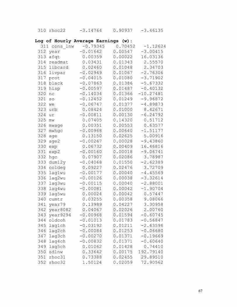
310 rhoc22 -3.14764 0.90937 -3.46135 Log of Hourly Average Earnings (w): 311 cons_lnw -0.79345 0.70452 -1.12624 312 year -0.01642 0.00547 -3.00415 313 afqt 0.00359 0.00022 16.03136 314 readmat 0.03431 0.01343 2.55570 315 libcard 0.02460 0.01048 2.34703 316 livpar -0.02949 0.01067 -2.76306 317 prot -0.04015 0.01080 -3.71902 318 black -0.07863 0.01386 -5.67332 319 hisp -0.00597 0.01487 -0.40132 320 nc -0.14034 0.01366 -10.27481 321 so -0.12452 0.01249 -9.96872 322 we -0.06747 0.01377 -4.89873 323 urb 0.08424 0.01000 8.42671 324 ur -0.00811 0.00130 -6.24792 325 mw 0.07405 0.14320 0.51712 326 mwage 0.00351 0.00553 0.63577 327 mwhgc -0.00968 0.00640 -1.51177 328 age 0.13150 0.02625 5.00916 329 age2 -0.00267 0.00028 -9.43860 330 exp 0.06732 0.00409 16.46816 331 exp2 -0.00160 0.00018 -9.06741 332 hgc 0.07907 0.02086 3.78987 333 dum12y -0.04068 0.01550 -2.62389 334 coldeg 0.09227 0.02476 3.72709 335 lag1wu -0.00177 0.00040 -4.45569 336 lag2wu -0.00126 0.00038 -3.32614 337 lag3wu -0.00115 0.00040 -2.88001 338 lag4wu -0.00081 0.00042 -1.90704 339 lag5wu 0.00024 0.00042 0.57447 340 cumtr 0.03255 0.00358 9.08066 341 year79 0.13989 0.04227 3.30958 342 year8082 0.04067 0.02026 2.00760 343 year9294 -0.00968 0.01594 -0.60745 344 oldcoh -0.01013 0.01783 -0.56847 345 lag1ch -0.03192 0.01211 -2.63596 346 lag2ch -0.00084 0.01253 -0.06680 347 lag3ch -0.00270 0.01371 -0.19669 348 lag4ch -0.00832 0.01371 -0.60640 349 lag5ch 0.01062 0.01428 0.74410 350 sdlnw 0.33642 0.00175 192.79140 351 rhoc31 0.73388 0.02455 29.89510 352 rhoc32 1.50124 0.02059 72.90562
67

Initial Schooling Level in 1979 (is): 353 cons_ini -5.70145 3.87557 -1.47113 354 mohgc 0.01863 0.00690 2.69980 355 fahgc 0.01844 0.00574 3.21460 356 sibnum -0.02429 0.00653 -3.72103 357 rbne 0.08320 0.08732 0.95281 358 rbnc 0.29234 0.09655 3.02799 359 rbso 0.02224 0.07750 0.28698 360 rbwe 0.22578 0.09657 2.33795 361 r14ne 1.02708 0.09308 11.03479 362 r14nc 0.78330 0.09515 8.23262 363 r14so 1.03586 0.08045 12.87626 364 r14we 1.10845 0.09235 12.00222 365 afqt 0.01262 0.00071 17.72058 366 readmat 0.19703 0.04181 4.71209 367 libcard 0.14383 0.04112 3.49746 368 livpar 0.05846 0.03765 1.55274 369 prot 0.06035 0.04388 1.37546 370 black 0.26490 0.04969 5.33104 371 hisp 0.11269 0.06146 1.83346 372 ugtuit 1.49251 0.63685 2.34358 373 expsec -0.47857 0.32260 -1.48349 374 expps -0.01924 0.18976 -0.10141 375 age 1.01264 0.43514 2.32714 376 age2 -0.01145 0.01230 -0.93044 377 age1415 -0.66638 0.18732 -3.55745 378 age16 -0.37201 0.11488 -3.23832 379 age17 -0.10472 0.07952 -1.31691 380 sdhgcini 0.92389 0.00732 126.24723 381 rhoc41 0.11976 0.13810 0.86726 382 rhoc42 0.32200 0.11723 2.74673
68

Heterogeneity Information: POINT PROB. WEIGHT MASS POINT FIRST PERMANENT HETEROGENEITY 1 0.02925 0.00000 2 0.08027 0.37403 3 0.32656 0.60835 4 0.44150 0.77702 5 0.12242 1.00000 SECOND PERMANENT HETEROGENEITY 1 0.12959 0.00000 2 0.35603 0.58521 3 0.48150 0.31993 4 0.03288 1.00000 NONLINEAR TRANSITORY HETEROGENEITY Any Schooling 1 0.17477 0.00000 2 0.03244 0.02102 3 0.01183 -0.12577 4 0.42026 0.22717 5 0.02763 -0.07135 6 0.33308 0.69062 Any Training 1 0.17477 0.00000 2 0.03244 -0.00446 3 0.01183 0.07182 4 0.42026 0.04399 5 0.02763 0.05970 6 0.33308 -0.05100 Any Work 1 0.17477 0.00000 2 0.03244 2.53530 3 0.01183 -3.18005 4 0.42026 -0.12075 5 0.02763 4.94166 6 0.33308 0.16036 Any Unemployment 1 0.17477 0.00000 2 0.03244 -0.04904 3 0.01183 -0.75519 4 0.42026 -4.95586 5 0.02763 -1.23314 6 0.33308 -1.22591 Any Job Change 1 0.17477 0.00000 2 0.03244 0.29726
69

3 0.01183 0.19501 4 0.42026 -2.23391 5 0.02763 -0.84130 6 0.33308 -99.00000 Hours worked 1 0.17477 0.00000 2 0.03244 -952.28885 3 0.01183 255.23279 4 0.42026 398.01243 5 0.02763 -76.58800 6 0.33308 96.74391 Weeks Unemployed 1 0.17477 0.00000 2 0.03244 15.27832 3 0.01183 27.98220 4 0.42026 21.25957 5 0.02763 0.00354 6 0.33308 -4.32722 Log Wage 1 0.17477 0.00000 2 0.03244 1.25946 3 0.01183 -3.60136 4 0.42026 0.04553 5 0.02763 -1.58095 6 0.33308 0.10578 Initial Schooling Level (no transitory heterogeneity) 1 0.17477 0.00000 2 0.03244 0.00000 3 0.01183 0.00000 4 0.42026 0.00000 5 0.02763 0.00000 6 0.33308 0.00000 ST. DEV. OF FIRST PERMANENT HETEROGENEITY: 0.19800532191946 ST. DEV. OF SECOND PERMANENT HETEROGENEITY:0.21874620581648 ST. DEV. OF NONLINEAR TRANSITORY HETEROGENEITY: Equation: 1 St. Dev. : 0.42531946262434 Equation: 2 St. Dev. : 4.2893100665523D-02 Equation: 3 St. Dev. : 1.0086913177151 Equation: 4 St. Dev. : 3.2971649614189 Equation: 5 St. Dev. : 57.154377787081 Equation: 6 St. Dev. : 316.29440007216 Equation: 7 St. Dev. : 14.595081582500 Equation: 8 St. Dev. : 0.52774440325561 Equation: 9 St. Dev. : 0.
70

REFERENCES
Angrist, Joshua, Guido Imbens and Donald Rubin (1996): “Identification of Causal Effects Using Instrumental Variables,” Journal of the American Statistical Association, 91(434), 444-455.
Becker, Brian and Stephen Hills (1980): “Teenage Unemployment: Some Evidence of the
Long-Run Effects,” Journal of Human Resources, 15, 354-372. Ben-Porath, Yoram (1967): “The Production of Human Capital and the Lifecycle of
Earnings,” Journal of Political Economy, 75, 352-365. Blinder, Alan and Yoram Weiss (1976): “Human Capital and Labor Supply: A
Synthesis,” Journal of Political Economy, 84, 449-472. Card, David and Thomas Lemieux (2000): “Adapting to Circumstances: The Evolution of
Work, School, and Living Arrangements among North American Youth,” in Blanchflower and Freeman (eds) Youth Employment and Joblessness in Advanced Countries, NBER and University of Chicago Press.
Cain, Glenn (1976): “The Challenge of Segmented Labor Market Theories to Orthodox
Theory: A Survey,” Journal of Economic Literature, 14(4), 1215-1253. Chamberlain, Gary (1980): “Analysis of Covariance with Qualitative Data,” Review of
Economic Studies, vol. 48, 225-238. Chamberlain, Gary (1984): “Panel Data,” in Griliches and Intriligator (eds) Handbook of
Econometrics Volume 2, North-Holland Press. Chamberlain, Gary (1985): “Heterogeneity, Omitted Variable Bias and Duration
Dependence,” in Heckman and Singer (eds) Longitudinal Analysis of Labour Market Data, Cambridge University Press.
Corcoran, Mary (1982): “The Employment and Wage Consequences of Teenage
Women's Nonemployment,” in Freeman and Wise (eds) The Youth Labor Market Problem: Its Nature, Causes and Consequences, NBER and University of Chicago Press.
Ellwood, David (1982): “Teenage Unemployment: Permanent Scars or Temporary
Blemishes?” in Freeman and Wise (eds) The Youth Labor Market Problem: Its Nature, Causes and Consequences, NBER and University of Chicago Press.
Freeman, Richard and James Medoff (1982): “The Youth Labor Market Problem in the
United States: An Overview,” in Freeman and Wise (eds) The Youth Labor Market Problem: Its Nature, Causes and Consequences, NBER and University of Chicago Press.
71

Flinn, Christopher and James Heckman (1982): “New Methods for Analyzing Structural Models of Labor Force Dynamics,” Journal of Econometrics, 18, 115-168.
---------- and ---------- (1983): “Are Unemployment and Out of the Labor Force
Behaviorally Distinct Labor Force States,” Journal of Labor Economics, 1(1), 28-42.
Freeman, Richard and James Medoff (1982): “The Youth Labor Market Problem in the
United States: An Overview,” in Freeman and Wise (eds) The Youth Labor Market Problem: Its Nature, Causes and Consequences, NBER and University of Chicago Press.
Freeman, Richard and David Wise (1982): “The Youth Labor Market Problem: Its
Nature, Causes and Consequences,” in Freeman and Wise (eds) The Youth Labor Market Problem: Its Nature, Causes and Consequences, NBER and University of Chicago Press.
Ghosh, Koushek (1994): “The Long-Run Impact of Early Employment Experience of
American Youth,” Ph.D. Thesis, Washington University at St. Louis. Gottschalk, Peter and Tim Maloney (1985): “Involuntary Terminations, Unemployment,
and Job Matching: A Test of Job Search Theory,” Journal of Labor Economics, 3(2), 109-123.
Greene, William H. (1993): “Econometric Analysis: Second Edition,” Prentice-Hall, Inc. Hausman, Jerry (1978): “Specification Tests in Econometrics,” Econometrica, 46, 1251-
1271. Heckman, James (1981): “Heterogeneity and State Dependence,” in Sherwin Rosen (ed)
Studies in Labor Markets, University of Chicago Press. -------------- (1990): “Varieties of Selection Bias,” American Economic Review, 80, 313-
318. Heckman, James and George Borjas (1980): “Does Unemployment Cause Future
Unemployment? Definitions, Questions and Answers from a Continuous Time Model of Heterogeneity and State Dependence,” Economica, 47, 247-283.
Heckman, James and Burton Singer (1984): “A Method for Minimizing the Impact of
Distributional Assumptions in Econometric Models for Duration Data,” Econometrica, 52, 271-320.
Lewis, H. Gregg (1986): “Union Relative Wage Effects: A Survey,” University of
Chicago Press.
72

Lippman, Steven and John McCall (1976): “The Economics of Job Search: A Survey,” Economic Inquiry, 14, 155-189.
Lynch, Lisa (1985): “State Dependency in Youth Unemployment: A Lost Generation?”
Journal of Econometrics, 28, 71-84. ---------- (1989): “The Youth Labor Market in the Eighties: Determinants of Re-
employment Probabilities for Young Men and Women,” The Review of Economics and Statistics, 71, 1, 37-45.
MaCurdy, Thomas, Thomas Mroz and Mark Gritz (1998): “An Evaluation of the NLSY,”
Journal of Human Resources, 33(2), 345-436. McLaughlin, Kenneth (1991): “A Theory of Quits and Layoffs with Efficient Turnover,”
Journal of Political Economy, 1991, 99(1), 1-29. Meyer, Robert and David Wise (1982): “High School Preparation and Early Labor Force
Experience,” in Freeman and Wise (eds) The Youth Labor Market Problem: Its Nature, Causes and Consequences, NBER and University of Chicago Press.
Meyer, Robert and David Wise (1983): “The Effects of the Minimum Wage on the
Employment and Earnings of Youth,” Journal of Labor Economics, 1(1), 66-100. ---------- and ---------- (1984): “The Transition from School to Work: The Experience of
Blacks and Whites,” Research in Labor Economics, Greenwich, Connecticut, JAI. Michael, Robert and Nancy Tuma (1984): “Youth Employment: Does Life Begin at 16?”
Journal of Labor Economics, 2, 4, 464-476. Mortensen, Dale (1970): “Job Search, The Duration of Unemployment and the Phillips
Curve,” American Economic Review, 72, 968-979. Mroz, Thomas (1999): “Discrete Factor Approximation in Simultaneous Equation
Models: Estimating the Impact of a Dummy Endogenous Variable on a Continuous Outcome,” Journal of Econometrics, 92(2), 233-74.
Mroz, Thomas and David Guilkey (1992): “Discrete Factor Approximations for Use in
Simultaneous Equation Models with Both Continuous and Discrete Endogenous Variables,” UNC Working Paper Series.
Mroz, Thomas and Brian Surette (1998): “Post-Secondary Schooling and Training
Effects on Wages and Employment,” UNC Working Paper Series. Narendranathan, Wiji and Peter Elias (1993): “Influences of Past History on the
Incidence of Youth Unemployment: Empirical Findings for the UK,” Oxford Bulletin of Economics and Statistics, 55, 161-185.
73

74
Neumark, David and William Wascher (1997): “Do Minimum Wages Fight Poverty?”
NBER Working Paper No. 6127. ---------- and ---------- (1996): “The Effects of Minimum Wages on Teenage Employment
and Enrollment: Evidence from Matched CPS Surveys,” Research in Labor Economics, 15, 25-63.
---------- and ---------- (1992): “Employment Effects of Minimum and Subminimum
Wages: Panel Data on State Minimum Wage Laws,” Industrial and Labor Relations Review, 46(1), 55-81.
Raphael, Steven (1996): “An Analysis of the Spatial Determinants and Long-Run
Consequences of Youth Joblessness,” Ph.D. Thesis, University of California at Berkeley.
Robinson, Chris (1989): “The Joint Determination of Union Status and Union Wage
Effects: Some Tests of Alternative Models,” Journal of Political Economy 97, 639-667.
Stevenson, W (1978): “The Relationship Between Early Work Experience and Future
Employability,” in Adams and Mangum (eds) The Lingering Crisis of Youth Unemployment, Kalamazoo.
Summers, Larry and Kim Clark (1982): “The Dynamics of Youth Unemployment,” in
Freeman and Wise (eds) The Youth Labor Market Problem: Its Nature, Causes and Consequences, NBER and University of Chicago Press.
US Department of Labor (2000): “Report on the Youth Labor Force.” Veum, Jonathan and Andrew Weiss (1993): “Education and the Work Histories of Young
Adults,” Monthly Labor Review, April 1993. Wolpin, Kenneth (1992): “The Determinants of Black-White Differences in Early
Employment Careers: Search, Layoffs, Quits, and Endogenous Wage Growth,” Journal of Political Economy, 100, 535-560.