Embed Size (px)
Citation preview
The Long-Term Effects of Financial Aid and Career
Education: Evidence from a Randomized Experiment
Job Market Paper.This version: January 9th, 2022. Click here for latest version.
Laëtitia Renée*
Abstract
I study the effects of the Future to Discover Project, a randomized experiment in
which Canadian high school students were either invited to participate in career
planning workshops or were made eligible for an $8,000 college grant. By matching
the experimental data to post-secondary institution records and income tax files, I am
able to examine the effects of the interventions on college enrollment, graduation, and
earnings in adulthood. I show that the career education intervention greatly improved
students’ outcomes in the long run by improving academic matching. In contrast, the
college grant had no long-term monetary benefits despite increasing college enrollment,
which is consistent with classical models of human capital investment in the absence
of credit constraints. My findings suggest that informational frictions and behavioral
obstacles—rather than financial constraints—represent the primary barrier to four-year
college enrollment faced by low-income students. And that they explain a large part of
the gap in four-year college enrollment between high- and low-income students. JEL
Codes: I22, I23, I24, D8, D31
*Department of Economics, McGill University, [email protected]. I am grateful to FabianLange and Fernando Saltiel for their continued guidance and support. I would also like to thank Sonia Laszlo,Christopher Rauh, Nicolas Gendron-Carrier, Stephen Ross, Andrei Munteanu, Marc Law, and participantsat the CIREQ Lunch Seminar, the 2021 Conferences of the ESPE, CEA, SOLE and EEA, the 2021 Summerand Winter Meetings of the Econometric Society, the GEEZ Seminar, the AMIE Workshop, and the RCIWorkshop for valuable input. I am indebted to the Social Research and Demonstration Corporation team,and especially to Reuben Ford, for research support and for making the Future to Discover project dataavailable via the Canadian Research Data Centre Network. I acknowledge the financial support of the Fondsdu Recherche du Quebec, the Quebec Interuniversity Centre for Social Statistics and the Research Initiative,Education + Skills. The analysis was conducted at the Quebec Interuniversity Centre for Social Statistics,part of the Canadian Research Data Centre Network. This service is provided through the support of QuebecUniversities, the province of Quebec, the Canadian Foundation for Innovation, the Canadian Institutes ofHealth Research, the Social Science and Humanity Research Council, the Fonds du Recherche du Québec,and Statistics Canada. All views expressed in this work are my own.
1 Introduction
Parental income is, across many countries, a strong predictor of post-secondary educa-tion enrollment.1 In part, this stems from differences in academic preparation betweenstudents from high- and low-income families. But large differences remain even aftercontrolling for academic achievement, raising concerns that students from low-incomefamilies might make sub-optimal educational choices due to financial, informational, orbehavioral barriers (Lochner and Monge-Naranjo (2012); French and Oreopoulos (2017)).
In response to these concerns, governments and other institutions invest large sumsin interventions promoting college access. These interventions can be broadly classifiedinto the two following categories: outreach and career counseling interventions aimed atimproving students’ decision-making regarding post-secondary education; and financialaid interventions designed to help students cover the costs of post-secondary education(Page and Scott-Clayton (2016); Herbaut and Geven (2020)).
Two key questions emerge from the literature: 1) are these interventions effectivein improving students’ outcomes in the long run? and 2) what type of intervention isthe most successful in doing so? While prior research has shown the effectiveness ofcareer counseling programs as well as financial aid interventions in increasing the collegeenrollment rate of low-income students, little is known about their long-term effects. Yet,that is not clear that an increase in enrollment will translate into an increase in graduationand earnings. Recent studies have demonstrated that educational interventions tend to“fade out” over time (Bailey et al. (2020)). In the case of interventions promoting collegeaccess, the “fade out” can occur because such interventions might induce students withlow expected returns to education to enroll in college.2
In this paper, I answer these questions by studying the short- and long-run impactsof the Future to Discover Project, a randomized control trial conducted between 2004and 2008 by the Social Research and Demonstration Corporation (SRDC). The projectselected 4,390 students from 30 high schools in New Brunswick (Canada) and randomlyassigned them to either a career education intervention, a financial aid intervention, amixed intervention, or a control group.
1. See, for example, Bailey and Dynarski (2011) and Chetty et al. (2014) for the US, Frenette (2017) forCanada, and Blossfeld and Shavit (1993) for twelve other countries. See Kinsler and Pavan (2011) and Hoxbyand Avery (2013) for the gap in enrollment in selective colleges.
2. For example, classical models of human capital investment predict that, by lowering the cost of college,financial aid provision would increase enrollment for students at the margin of enrolling, leading to weakeffects on long-term outcomes (Becker (1964)). Moreover, outreach programs can bias students’ beliefs abouttheir private returns to college enrollment leading to negative impacts of such interventions on long-termoutcomes.
2
Students assigned to the career education intervention were invited to participate intwenty career planning workshops, conducted from Grade 10 through Grade 12. Theseworkshops were designed to help students explore different post-secondary options,formulate their own post-secondary education plans in accordance with their interestsand skills, and develop strategies to achieve their goals. An important element of theintervention is that it provided guidance on post-secondary education decision-makingand application process, a dimension that has been found effective in raising collegeenrollment rates (Carrell and Sacerdote (2017)).
The financial aid was only randomized among students from low-income families.Students assigned to the financial aid intervention were eligible for a two-year $4,000 peryear grant conditional on post-secondary education enrollment. The grant was substantialas it covered most of the tuition costs of undergraduate studies at that time in NewBrunswick. Moreover, compared to existing financial aid programs, the interventionoffered an early guarantee of aid with a simple application process—two features that havebeen shown to enhance application rates (Bettinger et al. (2012); Dynarski et al. (2021)).
To study the long-term effects of the interventions, I match the experimental data toconfidential administrative data of post-secondary institution records and income tax files.The linked data allow me to investigate the causal impacts of the interventions on students’college enrollment, graduation, and earnings, from the end of high school through age 28.3
In addition, using the factorial design of the experiment—the fact that two interventionswere tested alone and combined—I can compare the relative effectiveness and synergy ofcareer education and financial aid in improving low-income students’ outcomes. To thebest of my knowledge the Future to Discover Project is the only experiment that allows todo so.
In the second part of the paper, I examine the role that the three interventions had inaligning high- and low-income students’ college enrollment and graduation rates. In par-ticular, I estimate the effects of the interventions on the gaps in enrollment and graduationbetween students with similar academic achievement prior to treatment. Because moststudies collect data on the specific group of students they are interested in, there is to date,little evaluation of the effects of such interventions on inequality.
I find that the career education intervention increased the share of low-income studentswho enrolled in four-year college by 8.3 percentage points. Going further, I find that itraised students’ earnings in adulthood. In particular, I estimate that by age 28 low-income
3. By matching the experimental data to administrative data I build on previous work conducted by theSRDC (see, for example, Ford et al. (2012) and Hui and Ford (2018)). Specifically, the data used by the SRDCdid not allow to accurately identify the impact of the interventions on college dropout and completion, andon earnings beyond age 24.
3
students assigned to the career education intervention earned 10% more on average in laborincome. It suggests that the intervention effectively improved students’ decision-makingregarding post-secondary education through the reduction in information frictions andbehavioral barriers (e.g., lack of attention and over-reliance on default options) targeted bythe program.4
In contrast, I do not find evidence that the college grant increased low-income students’earnings, although it substantially increased their community college enrollment andgraduation rates. One possible explanation for this finding, consistent with classicalmodels of human capital investment in the absence of credit constraints, is that the aidincreased enrollment and graduation for students whose expected benefits from enrollingare slightly smaller than the expected benefits of not doing so, leading to weak effects onlong-term outcomes (e.g., Becker (1964)).
Together these findings suggest that informational and behavioral obstacles, ratherthan financial constraints, represent the primary barrier to four-year college enrollmentfaced by low-income students.
I also explore the effects of the career education intervention on high-income students.I find that the intervention also had positive effects on their earnings in adulthood. Sugges-tive evidence indicates that part of this increase in earnings is driven by the interventioninducing students with a high risk of dropping out from college not to enroll. In fact, theintervention decreased the share of high-income students who enrolled in four-year collegeby 3.8 percentage points, but this effect is mostly driven by lower-achieving students and Ido not observe a similar decline in four-year college graduation.
It suggests that high-income students also suffer from information frictions and behav-ioral barriers. But while these obstacles lead some low-income students to academicallyunder-match, they lead some high-income students to academically over-match
By improving academic matching, the career education intervention completely alignedhigh- and low-income students’ four-year college enrollment behavior. In the controlgroup, low-income students were 13 percentage points less likely to enroll in a four-yearcollege than similarly-achieving high-income students. In the career education group, thegap is only 1 percentage point wide. It suggests that academic mismatch arising frominformational and behavioral barriers explain a large part of the gap in four-year collegeenrollment between the two types of students.
My paper makes several contributions to the literature. First, I contribute to thescarce literature on the long-term effects of interventions promoting college access. While
4. See French and Oreopoulos (2017) for a review of the possible informational and behavioral barriersstudents face transitioning to college.
4
previous research has shown the effectiveness of career counseling programs in increasingthe college enrollment rate of low-income students (e.g., Bettinger et al. (2012); Carrelland Sacerdote (2017); Castleman and Goodman (2018); Cunha, Miller, and Weisburst(2018); Oreopoulos and Ford (2019)), little is known about their long-term effects.5 I showthat career counseling programs are not only effective in increasing low-income students’college enrollment rates but are also powerful in improving students’ outcomes in the longrun.
The literature on the effects of student grant aid is more extensive. Numerous studieshave shown the effectiveness of these grants in increasing both college enrollment andcompletion (e.g., Fack and Grenet (2015); Castleman and Long (2016), Goldrick-Rab etal. (2016)), and a handful of recent evaluations have shown small but positive effects ofgrant aid on earnings (Bettinger et al. (2019), Denning, Marx, and Turner (2019); Scott-Clayton and Zafar (2019))6. However, the estimates of the treatment effects on earnings areoften imprecise and specific to the United States. My paper shows that providing studentswith additional financial support, in a country where a number of grants and loans arealready available to the students, has no long-term monetary benefits.
Second, I add to the understanding of the factors contributing to the gap in educationalattainment by parental income. To date, there is little consensus about the role playedby credit constraints (e.g., Keane and Wolpin (2001); Belley and Lochner (2007); Lochnerand Monge-Naranjo (2012)). Moreover, although recent studies have demonstrated theexistence of informational and behavioral barriers for low-income students (e.g., Bettingeret al. (2012); Hoxby and Avery (2013); Dynarski et al. (2021)), little is known on the extentto which they contribute to the gap. This paper provides new evidence that informationaland behavioral barriers explain most of the gap in four-year college enrollment betweenequally-achieving high- and low-income students.
More generally, my paper relates to the literature on the fading-out of educationalinterventions. As Bailey et al. (2020) explains, well-timed interventions introducing the“right” institutional changes are more likely to lead to persistent effects than interventionstargeting skills directly. Consistent with this finding, I find that the career educationintervention, which tackles informational and behavioral barriers, had large persistenteffects on graduation and earnings.
5. Two studies show promising results on degree completion. Bettinger et al. (2012) show that providingstudents with personal assistance for the FASFA application increased their likelihood to complete twoyears of college by 8 percentage points. In addition, Castleman and Goodman (2018) show that an intensivepost-secondary education counseling program substantially increased persistence throughout the third yearof college although this effect was not statistically significant.
6. See Eng and Matsudaira (2021) for an exception.
5
2 The Future to Discover Project
In this section, I draw on Currie et al. (2007) to describe the Future to Discover experiment.Throughout the paper, sample sizes are rounded to the nearest 10 for data confidentialityconcerns.
2.1 Context and Background
High school in New Brunswick, like in the US, runs from Grades 9 to 12, after whichstudents can decide whether to enroll in post-secondary education or not. Students aretypically 14 years old at the beginning of high school and graduate at age 18. Threemain options are available to students who want to enroll in post-secondary education inCanada: four-year colleges or universities (hereafter, four-year colleges) offering programsthat lead to a bachelor’s degree; community colleges, also referred to as colleges of appliedarts and technology or institutes of technology or science, which typically grant diplomasfor technical studies of two years; and private career colleges that offer career-orientedprograms of one year or less.
In Canada, the share of adults with a four-year college degree is nearly equal to 33percent, which is comparable to most developed countries (Statistics Canada (2020)).However, unlike other countries, Canada is characterized by a very high enrollmentrate in community and private career colleges: 26 percent of Canadian adults have ashort-cycle tertiary diploma compared to 7 percent of adults in other OECD countries(Statistics Canada (2020)). The high enrollment rate in post-secondary education maskslarge disparities. A young Canadian adult from a family in the bottom income quintile is30 percent less likely to attend a post-secondary institution than someone from a family inthe top income quintile (Belley, Frenette, and Lochner (2014); Frenette (2017)).
2.2 Experimental Design
The Future to Discover project was designed and implemented by the SRDC with thesupport of Statistics Canada.7 With the objective of finding out what works best to increasecollege enrollment, three interventions targeted to high school students were designedand tested in the Canadian province of New Brunswick, namely, a career educationintervention, a financial aid intervention, and a mixed intervention.
7. The SRDC is a non-profit research organization based in Ottawa, Canada. The experiment receivedfinancial support from the Canada Millennium Foundation.
6
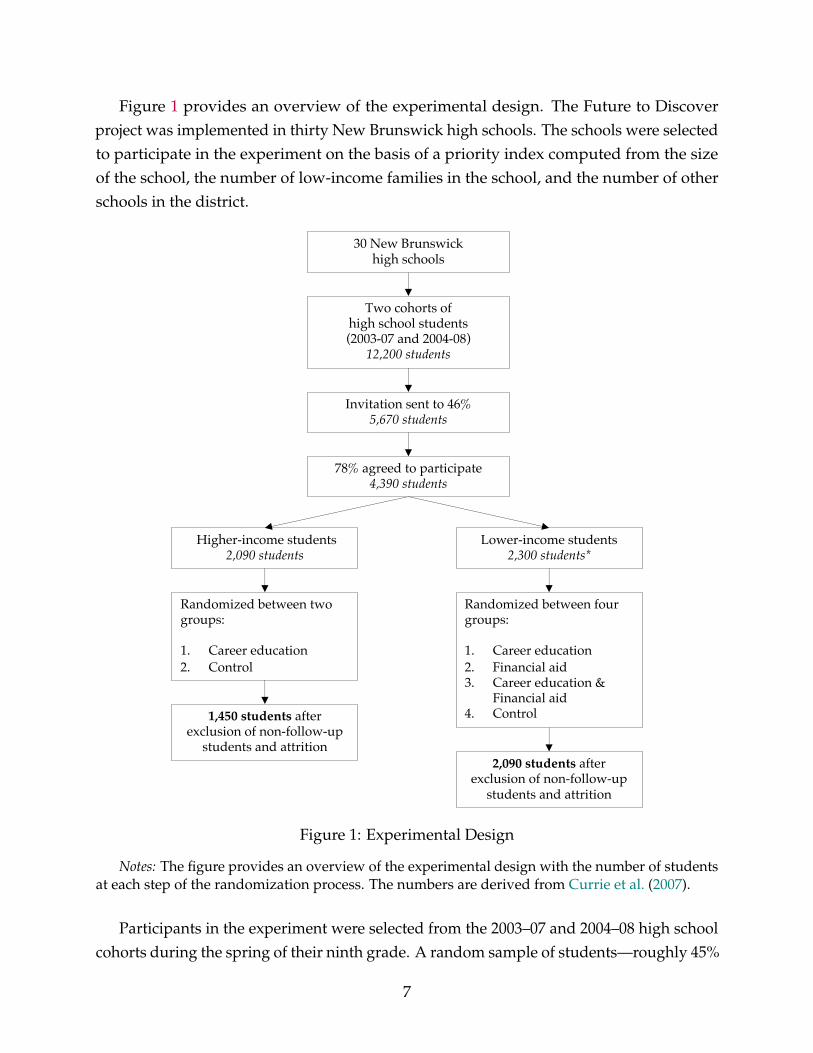
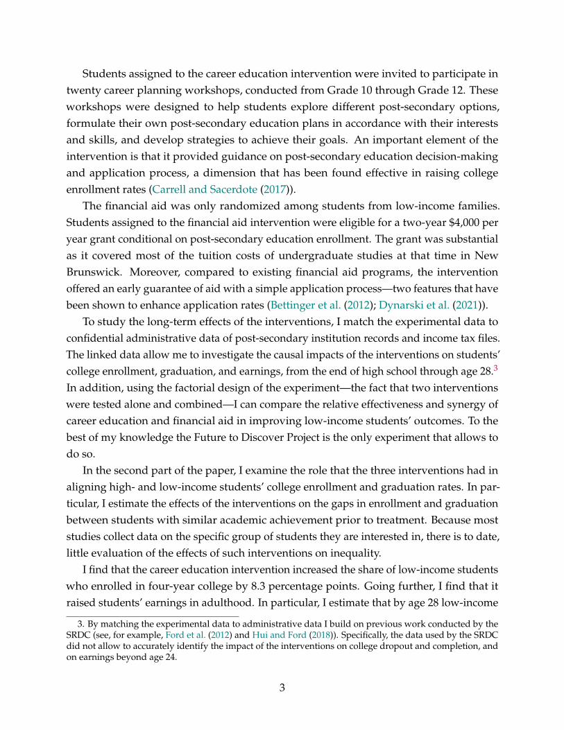
Figure 1 provides an overview of the experimental design. The Future to Discoverproject was implemented in thirty New Brunswick high schools. The schools were selectedto participate in the experiment on the basis of a priority index computed from the sizeof the school, the number of low-income families in the school, and the number of otherschools in the district.
30 New Brunswick high schools
Two cohorts of high school students (2003-07 and 2004-08)
12,200 students
Lower-income students2,300 students*
Higher-income students2,090 students
Randomized between two groups:
1. Career education2. Control
Randomized between four groups:
1. Career education2. Financial aid3. Career education &
Financial aid4. Control
Invitation sent to 46%5,670 students
78% agreed to participate4,390 students
1,450 students after exclusion of non-follow-up
students and attrition2,090 students after
exclusion of non-follow-up students and attrition
Figure 1: Experimental Design
Notes: The figure provides an overview of the experimental design with the number of studentsat each step of the randomization process. The numbers are derived from Currie et al. (2007).
Participants in the experiment were selected from the 2003–07 and 2004–08 high schoolcohorts during the spring of their ninth grade. A random sample of students—roughly 45%
7
or 5,670 students—was initially chosen among the freshmen cohorts to receive invitationsto participate in the experiment. Upon invitation, students along with their parents, wererequired to give their written consent and answer the baseline survey in order to take partin the experiment. These requirements were fulfilled by about 78 percent of the studentsinvited to participate.
During the baseline interview, the answering parent was asked to provide the annualhousehold income as stated in his previous year’s income tax returns. If the amount earnedwas above the provincial median, the student was classified as a high-income student andas a low-income student otherwise.8 Low-income students were randomly assigned to thethree treatment arms (career education, financial aid, mixed intervention) and the controlgroup. High-income students were not eligible for financial aid and were accordingly onlyrandomized between the career education and control groups. The randomization wasconducted at the student level within each school.9
Tables A3 and A4 show baseline descriptive statistics (mean and standard deviation) forlow- and high-income students in the control group, and report the differences between thecontrol group and the treatment groups. The table shows a balance on almost all baselinecharacteristics. I find four significant differences out of 56 tests, a number that could havebeen obtained by chance alone. In addition, I test for whether the baseline characteristicsjointly predict treatment status. I find no evidence that the baseline characteristics jointlypredict treatment status for both high- and low-income students (p-value from F-test is0.55 for low-income students and 0.95 for high-income students).
2.3 Career Education Program
Students assigned to the career education program were invited to participate in twentycareer planning workshops, conducted from Grade 10 through Grade 12. The workshopswere split into the following four series:
1. Career Focusing—The first workshop series was conducted in Grade 10. It includedsix workshops that were designed to guide students into the exploration of career op-
8. The threshold varied with family size. Six thresholds were defined, ranging from $40,000 for a single-parent family with one child to $60,000 for a family with two parents and three children or more.
9. Due to budgetary concerns the assignment ratios were adjusted for the second cohort of students,and a small random sample of students was excluded from the data collection. While the differentialtreatment assignment ratios across cohorts could lead to a complex empirical analysis design, the exclusionof students was conducted so as to equalize the assignment ratios across the two cohorts, allowing for astraightforward pooling of the students in the analysis. Although some administrative data are availablefor the non-follow-up students, I follow previous studies (Ford et al. (2012), Ford and Kwakye (2016), andHui and Ford (2018)) and exclude them from my analysis. Table A1 presents the distribution of the studentsacross parental income and the four randomization groups.
8

tions. Besides being taught how to research information on post-secondary educationand labor market trends, students were encouraged to explore their post-secondaryoptions through different activities and exercises.
2. Lasting Gifts—The second workshop series, which took place in Grade 11, wastailored toward the parents. The four workshops of the series aimed to encourageand assist the parents in getting involved in their children’s career planning. Togetherwith their children, parents were exposed to various career-planning approaches andwere instructed to test these approaches through interactive activities and reflectiveexercises.
3. Future in Focus—The third workshop series was designed to help Grade 12 studentsbuild resilience to overcome unexpected life challenges. The workshops focusedon the specific skills and attitudes needed to work through obstacles and on theimportance of developing a support network.
4. Post-secondary Ambassadors—Six meetings with post-secondary education studentsfrom various institutions were organized over Grades 10 to 12. The invited studentswere asked to share their experiences and advice, providing high school studentswith peer mentors and role models.
The workshops were held on each school property right after school hours, with theexception of the second workshop series, which took place in the evening to facilitate theparticipation of the parents. From the randomization, 30 to 35 students were typicallyinvited to the workshops in each school, allowing the meetings to be held in a classroomand facilitating interactions. The workshops were optional. Students were actively re-minded about the date and location of the workshops through text messages, mails, andannouncements in each school. They were also encouraged to attend through prizes andsnacks.
In addition, students were given access to post-secondary and career information viaa website and a magazine.10 The two media shared the same content—a description ofpost-secondary options, a guide to the financial aid system, labor market trends, and linksto other career education resources. The same content was offered across the two media inorder to reach more students and parents with different habits and access to the internet.
The career education program can theoretically have several effects on students’ col-lege enrollment and earnings. On the one hand, the program can improve students’
10. Six issues of the magazine were sent to the students over Grades 10 to 12. To limit spillover, the websitewas restricted to treated students only via a unique access key. Students received their login informationwith the magazine’s first issue and could access the website anytime from then on.
9
decision-making regarding post-secondary education by tackling several informationaland behavioral barriers students might face. First, by pushing students to look for infor-mation on the costs and benefits of each post-secondary option, the program is expectedto reduce misinformation. Second, by helping students think about their options andunderstand the long-lasting effects of their choices, it might minimize students’ lack ofattention, present bias, and over-reliance on default options—three behavioral barriers thathave be found to be important in students’ educational decisions (French and Oreopoulos(2017)). An improvement in decision-making can result, in turn, in an increase or to adecrease in college enrollment depending on the direction of the initial mistakes made bythe students. It should however lead to an improvement in students’ outcomes in the longrun.
On the other hand, the program can bias students’ beliefs about their private returns tocollege enrollment, leading to an increase in enrollment but negative effects on studentslong-run outcomes. That will be the case if, for instance, it pushes students to enroll infour-year college programs regardless of their academic ability.
2.4 Financial Aid
Students assigned to the financial aid intervention were eligible for a college grant worthup to $8,000. They could claim $2,000 each academic term they enrolled in post-secondaryeducation, for a period of four terms or two years.11 They were informed about the grantat the time of recruitment in Grade 9 and reminded about it at the end of Grade 12 andone year after high school.
The financial aid was substantial compared to tuition fees at the time of the experiment.Between 2007 and 2011, when most students from the sample enrolled in post-secondaryeducation, tuition fees in New Brunswick for one year of undergraduate schooling wereroughly equal to $5,500 in four-year colleges and $2,300 in community colleges.12
The financial intervention can affect students’ outcomes in two ways. On the onehand, by reducing the amount students need to borrow to finance their education, theintervention might reduce financial barriers such as credit constraints and debt aversion.In that case, we would expect an increase in enrollment and an improvement in students’long-run outcomes. On the other hand, classical models of human capital investment
11. To receive the grant, students had to register in a post-secondary program recognized by the CanadaStudent Loans Program. It includes most four-year and vocational programs as long as they lead to acertificate, diploma, or degree. Students were eligible to receive the payments for three years after highschool graduation.
12. Tuition fees from the four main four-year colleges were retrieved from Statistics Canada: Table 37-10-0045-01 Canadian and international tuition fees by level of study.
10
predict that the aid, by lowering the cost of college, would increase enrollment for studentswhose expected benefits from enrolling are slightly smaller than the expected benefits ofnot enrolling, resulting in limited benefits in the long run.
3 Empirical Framework
3.1 Data
I use data from three main sources.
1. Experimental Data—First, I obtained data from the SRDC on (i) students’ character-istics collected through the baseline survey conducted in Grade 9 (demographics,family composition, socioeconomic status and aspirations); (ii) students’ participa-tion in the workshops and their claims to the financial aid; and (iii) student test scoresand high school graduation.
2. Canadian Post-Secondary Information System—Second, I matched the experimental dataobtained from the SRDC to the Canadian Post-Secondary Information System, whichprovides information on enrollment and graduation for the universe of students whoattended a public post-secondary institution in Canada from the 2000–01 academicyear to the 2017–18 academic year, allowing me to observe post-secondary educationtrajectories in public institutions until age 28 for both cohorts.13
3. Statistics Canada Tax Filer Database—The experimental data were also matched toearnings data from the Statistics Canada confidential tax filer database. The databaseprovides information on earnings (labor income, total earnings) for all individualswho filed a tax return during a reference year. Because Canada requires anyone whoowes taxes or qualifies for refunds or credits to file a tax return, the majority of adults,including post-secondary students, generally file a tax return every year, irrespectiveof their working status.
These data suffer from two limitations that I address in different ways. First, I cannotestimate the impact of the interventions on enrollment and graduation from private
13. The system aims to cover the universe of public post-secondary institutions. However, only 95 percentof these institutions are indeed covered (even fewer before 2009, when only 80 percent were covered bythe system). In New Brunswick specifically, the platform does not cover the New Brunswick CommunityCollege—one of the two largest community colleges in New Brunswick—before 2010. This is challenging asI expect most of the impact of the program to happen from 2007 to 2009. To recover data from this institution,I supplement the platform until 2010 with data on enrollment and graduation gathered by the SRDC fromthe New Brunswick Department of Post-secondary Education, Training, and Labour.
11
institutions. This is likely a small limitation for the identification of enrollment andgraduation from four-year and community colleges as they are nearly all public-funded.Only a few private, most of which are faith-based, four-year colleges exist, and they attracta tiny fraction of students (Jones and Li (2015)). However, a number of small privatecareer colleges, which offer short and career-oriented programs of one year or less, arenot captured by the administrative data. To identify the impact of the interventions onenrollment in these types of institutions, I rely on the survey conducted two and a halfyears after high school graduation. The survey is, however, conducted too soon to providea reliable view of graduation.
Second, I do not observe earnings data beyond age 24 for the students who neverenrolled in a public post-secondary institution or registered as an apprentice (34 percentof the sample). This stems from the fact that the link with earnings data was done in twowaves. First, earnings until age 24 were initially acquired by the SRDC for all studentsin the sample. Second, earnings until age 28 were retrieved for students who enrolledin a public post-secondary institution or registered as an apprentice via the CanadianEducation and Labour Market Longitudinal Platform. I address this limitation by imputingthe missing data. Section 3.3 provides more details on the methodology used.
Appendix Section B summarizes the timeline of data coverage and details the construc-tion of the outcomes of interest.
3.2 Analytic Samples
I exclude 49 students from the sample for whom less than two years of earnings data isavailable, suggesting that they might have moved out of the country or that their SocialInsurance Number used to match the administrative data could not be relied upon. Thesestudents account for 1.4 percent of the initial sample. I find no evidence that the attritionrate differs by treatment group, as shown in Table A2. In Table A5 and A6, I also ensurethat baseline characteristics remain balanced across treatment groups after excludingthese students. In total, my sample is composed of 2,090 low-income students and 1,450high-income students.
I further restrict my sample when looking at specific secondary outcomes for whichdata is not available for all students. It is the case for high school graduation and averagetest scores in Grade 12 that was not provided for all students, most likely because somestudents dropped out or transferred to another school.14 This is also true for enrollment in
14. Test scores in Grade 12 are available for 80 percent of the low-income students and 91 percent of thehigh-income students. Graduation data are available for 87 percent of the low-income students and 94percent of the high-income students.
12
private institutions for which I only have data for students who answered the survey.15 Itest and discuss potential threats to causal identification arising from selective missingnesswhen presenting the results on these outcomes. Moreover, to enable the comparisonof the treatment effects measured on the restricted samples with the ones measuredfrom the full sample, I adjust the treatment effects on these outcomes using inverseprobability weighting (IPW) (Seaman and White (2013)). This method puts more weight onobservations that have, according to observed baseline characteristics, a high probabilityto be missing for the outcome of interest but are not. In practice, I construct the weightsfrom Probit regressions of the missingness indicators on treatment dummies, baselinecharacteristics, and cohort and school dummies.
3.3 Imputation of Earnings Data
I seek to study the impact of the interventions on earnings at different ages, starting fromage 19, when most students have left high school, until the age of 28, the most recent yearfor which I have data on earnings.
Earnings data may be missing for two reasons (Table A7). First, as explained in thedata section, earnings data were not collected beyond age 24 for students who did notenroll in a public post-secondary institution. This is the case for roughly 1,210 students,or 34 percent of the entire sample. Second, over the period for which earnings data werecollected, earnings records are missing for students who did not file a tax return duringthe reference year or filed the return too late. It is the case for 6 percent of the records.
To estimate the effects of the interventions on earnings, I need to account for thesemissing values. I address the issue by imputing the missing records rather than byrestricting the sample to complete cases, which would lead to a loss of power and biases. Ideal with the two types of missing values in different ways. First, I impute the missingrecords found over the period data were collected using linear interpolations from theavailable records of each individual.16 Second, I forecast the earnings from age 25 toage 28 for each student whose data were only collected until age 24. For this purpose,I estimate a model which takes into account the students’ past earnings records, theircurrent level of education and years of experience and whether they are currently enrolledin post-secondary education.
I formally describe the linear interpolation method and the forecasting procedure inAppendix Section C.
15. 87 percent of the low-income students and 95 percent of the high-income students answered the survey.16. The data restriction mentioned above ensure that I observe at least two years of earnings data points
for each individual, making sure the interpolation is feasible for each individual.
13
3.4 Empirical Strategy
I first focus on the effect of the three interventions on low-income students. To recover thetreatment effects, I estimate the following equation by Ordinary Least Squares (OLS),17
Yi = β0 + β1Ci + β2Fi + β3Mi + β4Xi + β5Si + εi (1)
with Yi is the outcome of interest for student i, C is a binary indicator equal to one if studenti was assigned to the career education only group, F is a binary indicator equal to one ifstudent i was assigned to the financial aid only group, and M is a binary indicator equal toone if student i was assigned to the mixed intervention group. Xi is a vector of baselinecharacteristics for student i and Si is a vector of school-cohort dummies corresponding tothe level of stratification.18
I follow the common practice of adjusting the results with the inclusion of baselinecharacteristics. I explore the sensitivity of the results to the exclusion of covariates in TablesA8, A9, and A10. The results do not significantly change when controls are removed,except for the treatment effects of the career education program on low-income studentsthat are larger. I also report in the same table the results from the regressions whererelevant controls are selected using the post-double-selection lasso method developed byBelloni, Chernozhukov, and Hansen (2013).19 The treatment effects are virtually identicalwhen controls are selected following the post-double-selection lasso method to when theyare not.
The β1 and β3 coefficients capture the effects of eligibility for the career educationprogram alone and combined with a financial nudge, respectively. Participation in theprogram was not compulsory—students were neither compelled to attend the workshop orto read the magazine/visit the website. However, note that nearly all students assigned totreatment were exposed to the program if we consider all forms of exposure. Among thoseassigned to treatment, 85 percent attended at least one workshop, 73 percent declaredhaving read parts of the magazine, and 22 percent visited the website. In what follows, I usethe terms “eligibility for the career education program” and “career education intervention”
17. I estimate the same linear model for both continuous and binary outcomes. Although a linear probabilitymodel can yield fitted values being outside the unit interval, it produces unbiased estimates of the averageeffects (Wooldridge (2010)).
18. The baseline characteristics included in the regression are all variables in Table A3, namely, gender,language spoken at home, whether one parent was born outside Canada, household composition, level ofeducation of parents, whether student wants a four-year college degree and test score dummies.
19. The selection procedure chooses variables from the set of characteristics listed in Table A3 and theirinteractions that are significant predictors of either the outcome of interest Yi or any of the treatment variablesof interest, Ci, Fi, and Mi (Belloni, Chernozhukov, and Hansen (2013)).
14
interchangeably.Since the intervention is randomized at the individual level in each school, I cannot rule
out spillover effects. Spillover might have occurred in two ways. First, students from thecareer education group might have shared information they learned during the workshopsor from the website and the magazine. They might have even lent the magazine or sharedtheir login information with other students. Second, by changing the students’ enrollmentbehavior, the program might have influenced students in the control group through peereffects. Assuming that the spillover effects, if any, would play in the same direction as ofthe direct effects, the impacts I estimate are lower bounds for the true impacts.
I report in all tables Huber–White robust standard errors and standard sampling-basedsignificance levels. In addition, I report in Tables A11 and A12, randomization-basedFisher-exact p-values for the main outcomes of interest. These p-values do not rely onasymptotic properties but on the random assignment itself (Heß (2017), Young (2019)). Ifind that the exact p-values are virtually identical to the sampling-based p-values which isexplained by the fact that the samples used are not small. I also address in the same tablepotential concerns arising from multiple hypothesis testing by computing sharpened q-values which control for the False Discovery Rate (Benjamini, Krieger, and Yekutieli (2006),Anderson (2008)). Most of the effects (72 percent) found to be significant using sampling-based significance levels survive multiple hypothesis testing correction. I indicate belowwhen they do not.
I am also interested in understanding the treatment effects of eligibility for the careereducation program on high-income students as well as in the difference in effects betweenhigh- and low-income students. I thus estimate the following equation by OLS, on therestricted sample of students assigned to the control or career education groups,
Yi = γ0 + γ1HIi + γ2Ci + γ3Ci × HIi + γ4Xi + γ5Si + υi, (2)
where HIi is a binary indicator equal to one if student i is a high-income student and 0otherwise. γ2 measures the treatment effect on low-income students, the sum of γ2 andγ3 the treatment effect on high-income students and γ3 the treatment effect on the gap inoutcome between the two types of students.
Additional specifications are used and described in the results section.
15
4 Results
4.1 Effects of the Career Education and Financial Aid Interventions on
Low-Income Students’ Outcomes
I first focus on the effects of eligibility for the career education program and eligibility forthe college grant on low-income students’ outcomes.
High school Graduation and Academic Performance
By changing students’ post-secondary education aspirations, the interventions might haveinfluenced students’ effort and graduation plans. Therefore, I begin by exploring the effectsof the interventions on high school graduation and academic performance in Table A13.The two interventions had no meaningful effects on students’ academic performance asmeasured by average test scores in Grade 12, or on the fraction of students who graduatedfrom high school. As a result, any effects observed in the next section on college enrollmentare more likely to result from a change in aspiration than from a change in performance.
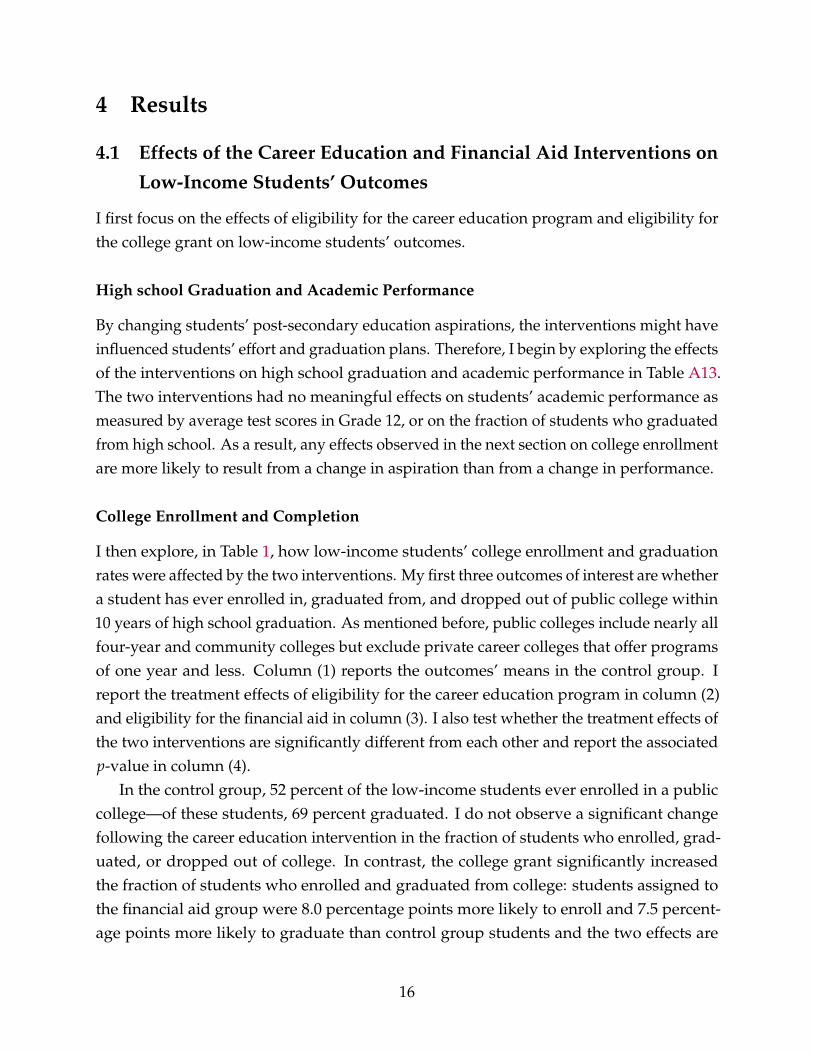
College Enrollment and Completion
I then explore, in Table 1, how low-income students’ college enrollment and graduationrates were affected by the two interventions. My first three outcomes of interest are whethera student has ever enrolled in, graduated from, and dropped out of public college within10 years of high school graduation. As mentioned before, public colleges include nearly allfour-year and community colleges but exclude private career colleges that offer programsof one year and less. Column (1) reports the outcomes’ means in the control group. Ireport the treatment effects of eligibility for the career education program in column (2)and eligibility for the financial aid in column (3). I also test whether the treatment effects ofthe two interventions are significantly different from each other and report the associatedp-value in column (4).
In the control group, 52 percent of the low-income students ever enrolled in a publiccollege—of these students, 69 percent graduated. I do not observe a significant changefollowing the career education intervention in the fraction of students who enrolled, grad-uated, or dropped out of college. In contrast, the college grant significantly increasedthe fraction of students who enrolled and graduated from college: students assigned tothe financial aid group were 8.0 percentage points more likely to enroll and 7.5 percent-age points more likely to graduate than control group students and the two effects are
16
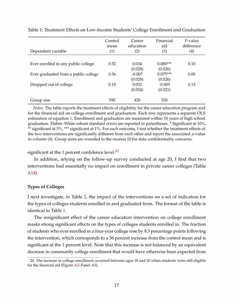
Table 1: Treatment Effects on Low-Income Students’ College Enrollment and Graduation
Controlmean
Careereducation
Financialaid
P-valuedifference
Dependent variable (1) (2) (3) (4)
Ever enrolled in any public college 0.52 0.034 0.080*** 0.10(0.028) (0.026)
Ever graduated from a public college 0.36 -0.007 0.075*** 0.00(0.028) (0.026)
Dropped out of college 0.15 0.032 -0.003 0.15(0.024) (0.021)
Group size 590 420 530
Notes: The table reports the treatment effects of eligibility for the career education program andfor the financial aid on college enrollment and graduation. Each row represents a separate OLSestimation of equation 1. Enrollment and graduation are measured within 10 years of high schoolgraduation. Huber–White robust standard errors are reported in parentheses. * Significant at 10%,** significant at 5%, *** significant at 1%. For each outcome, I test whether the treatment effects ofthe two interventions are significantly different from each other and report the associated p-valuein column (4). Group sizes are rounded to the nearest 10 for data confidentiality concerns.
significant at the 1 percent confidence level.20
In addition, relying on the follow-up survey conducted at age 20, I find that twointerventions had essentially no impact on enrollment in private career colleges (TableA14).
Types of Colleges
I next investigate, in Table 2, the impact of the interventions on a set of indicators forthe types of colleges students enrolled in and graduated from. The format of the table isidentical to Table 1.
The insignificant effect of the career education intervention on college enrollmentmasks strong significant effects on the types of colleges students enrolled in. The fractionof students who ever enrolled in a four-year college rose by 8.3 percentage points followingthe intervention, which corresponds to a 36 percent increase from the control mean and issignificant at the 1 percent level. Note that this increase is not balanced by an equivalentdecrease in community college enrollment that would have otherwise been expected from
20. The increase in college enrollment occurred between ages 18 and 20 when students were still eligiblefor the financial aid (Figure A2–Panel A3).
17
Table 2: Treatment Effects on the Type of College Low-Income Students Enrolled in andGraduated from
Controlmean
Careereducation
Financialaid
P-valuedifference
Dependent variable (1) (2) (3) (4)
Panel A—Enrollment
First enrolled in a four-year college 0.21 0.057** 0.030 0.26(0.023) (0.021)
First enrolled in a community college 0.31 -0.017 0.048* 0.03(0.028) (0.027)
Switched to a community college 0.06 0.009 0.015 0.72(0.016) (0.014)
Switched to a four-year college 0.02 0.028** 0.002 0.02(0.011) (0.008)
Ever enrolled in a four-year college 0.23 0.083*** 0.032 0.04(0.024) (0.021)
Ever enrolled in a community college 0.36 -0.012 0.065** 0.01(0.030) (0.028)
Panel B—Graduation
Four-year college degree 0.14 0.037* -0.003 0.07(0.021) (0.018)
Community college diploma 0.24 -0.033 0.076*** 0.00(0.027) (0.026)
Panel C—Dropout
Dropped out of a four-year college 0.08 0.041** 0.026 0.46(0.020) (0.017)
Dropped out of a community college 0.08 0.019 -0.017 0.09(0.021) (0.018)
Group size 590 420 530
Notes: The table reports the treatment effects of eligibility for the career education programand for the financial aid on the type of college students enrolled in and graduated from. Eachrow represents a separate OLS estimation of equation 1. Enrollment and graduation are measuredwithin 10 years of high school graduation. Huber–White robust standard errors are reported inparentheses. * Significant at 10%, ** significant at 5%, *** significant at 1%. For each outcome, I testwhether the treatment effects of the two interventions are significantly different from each otherand report the associated p-value in column (4). Group sizes are rounded to the nearest 10 for dataconfidentiality concerns.
the null effect on any college enrollment.21
21. In line with these results, I find that eligibility for the career education program increased the fraction
18
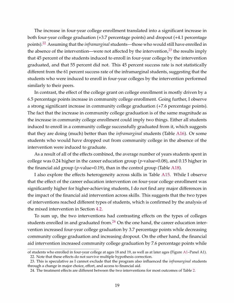
The increase in four-year college enrollment translated into a significant increase inboth four-year college graduation (+3.7 percentage points) and dropout (+4.1 percentagepoints).22 Assuming that the inframarginal students—those who would still have enrolled inthe absence of the intervention—were not affected by the intervention,23 the results implythat 45 percent of the students induced to enroll in four-year college by the interventiongraduated, and that 55 percent did not. This 45 percent success rate is not statisticallydifferent from the 61 percent success rate of the inframarginal students, suggesting that thestudents who were induced to enroll in four-year colleges by the intervention performedsimilarly to their peers.
In contrast, the effect of the college grant on college enrollment is mostly driven by a6.5 percentage points increase in community college enrollment. Going further, I observea strong significant increase in community college graduation (+7.6 percentage points).The fact that the increase in community college graduation is of the same magnitude asthe increase in community college enrollment could imply two things. Either all studentsinduced to enroll in a community college successfully graduated from it, which suggeststhat they are doing (much) better than the inframarginal students (Table A16). Or somestudents who would have dropped out from community college in the absence of theintervention were induced to graduate.
As a result of all of the effects combined, the average number of years students spent incollege was 0.24 higher in the career education group (p-value=0.08), and 0.15 higher inthe financial aid group (p-value=0.19), than in the control group (Table A18).
I also explore the effects heterogeneity across skills in Table A15. While I observethat the effect of the career education intervention on four-year college enrollment wassignificantly higher for higher-achieving students, I do not find any major differences inthe impact of the financial aid intervention across skills. This suggests that the two typesof interventions reached different types of students, which is confirmed by the analysis ofthe mixed intervention in Section 4.2.
To sum up, the two interventions had contrasting effects on the types of collegesstudents enrolled in and graduated from.24 On the one hand, the career education inter-vention increased four-year college graduation by 3.7 percentage points while decreasingcommunity college graduation and increasing dropout. On the other hand, the financialaid intervention increased community college graduation by 7.6 percentage points while
of students who enrolled in four-year college at ages 18 and 19, as well as at later ages (Figure A1–Panel A1).22. Note that these effects do not survive multiple hypothesis correction.23. This is speculative as I cannot exclude that the program also influenced the inframarginal students
through a change in major choice, effort, and access to financial aid.24. The treatment effects are different between the two interventions for most outcomes of Table 2.
19
having no adverse effect on dropout.From these results alone, it is unclear what will be the effects of the two interventions
on students’ long-term outcomes. These effects will ultimately depend on the returnsto four-year and community college graduation for the marginal students, and on themagnitude of the adverse effects of college dropout.
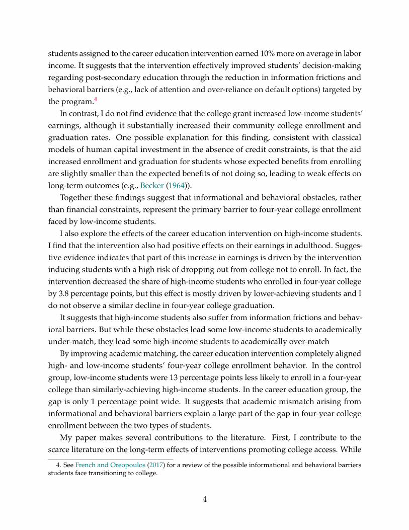
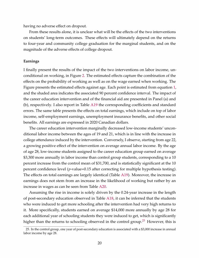
Earnings
I finally present the results of the impact of the two interventions on labor income, un-conditional on working, in Figure 2. The estimated effects capture the combination of theeffects on the probability of working as well as on the wage earned when working. TheFigure presents the estimated effects against age. Each point is estimated from equation 1,and the shaded area indicates the associated 90 percent confidence interval. The impact ofthe career education intervention and of the financial aid are presented in Panel (a) and(b), respectively. I also report in Table A19 the corresponding coefficients and standarderrors. The same table presents the effects on total earnings, which include on top of laborincome, self-employment earnings, unemployment insurance benefits, and other socialbenefits. All earnings are expressed in 2020 Canadian dollars.
The career education intervention marginally decreased low-income students’ uncon-ditional labor income between the ages of 19 and 21, which is in line with the increase incollege attendance induced by the intervention. Conversely, I observe, starting from age 22,a growing positive effect of the intervention on average annual labor income. By the ageof age 28, low-income students assigned to the career education group earned on average$3,300 more annually in labor income than control group students, corresponding to a 10percent increase from the control mean of $31,700, and is statistically significant at the 10percent confidence level (p-value=0.15 after correcting for multiple hypothesis testing).The effects on total earnings are largely identical (Table A19). Moreover, the increase inearnings does not stem from an increase in the likelihood of working but rather by anincrease in wages as can be seen from Table A20.
Assuming the rise in income is solely driven by the 0.24-year increase in the lengthof post-secondary education observed in Table A18, it can be inferred that the studentswho were induced to get more schooling after the intervention had very high returns toit. More specifically, students earned on average $14,000 more annually by age 28 foreach additional year of schooling students they were induced to get, which is significantlyhigher than the returns to schooling observed in the control group.25 However, this is
25. In the control group, one year of post-secondary education is associated with a $3,000 increase in annuallabor income by age 28.
20
(a) Career education intervention
−4,000
−2,000
0
2,000
4,000
6,000
8,000
19 20 21 22 23 24 25 26 27 28Age
Trea
tmen
t eff
ects
on
labo
r in
com
e ($
CA
)(b) Financial aid intervention
−4,000
−2,000
0
2,000
4,000
6,000
8,000
19 20 21 22 23 24 25 26 27 28Age
Trea
tmen
t eff
ects
on
labo
r in
com
e ($
CA
)Figure 2: Impact on Labor Income Over Time
Notes: The figure plots the effects of eligibility for the career education program and for thefinancial aid on labor income against age. Point estimates together with the associated 90 percentconfidence intervals are reported. Each point is estimated from a separate OLS estimation ofequation 1. Huber–White robust standard errors are used to compute the confidence intervals.Earnings are expressed in 2020 Canadian dollars.
only suggestive as I cannot empirically rule out that other channels drove the increase inearnings, such as changes in major or occupational choices.
These findings imply that the intervention did lower the barriers students encounteredin maximizing earnings. Since the intervention only changed students’ decision-makingprocess but not the environment they actually faced, it highlights the existence of informa-tional and behavioral barriers for some students.
The decrease in labor income between the ages of 19 and 21 induced by the careereducation intervention is also observed with the financial aid treatment since they bothhad similar effects on college enrollment. Surprisingly, the financial aid interventionhad no noticeable effect on labor income and total earnings beyond age 22, although itsubstantially increased graduation from community colleges. The lack of effect suggeststhat students were induced to enroll in and graduate from programs with on averagelimited monetary returns.
One possible explanation for this finding is that the aid increased enrollment andgraduation for students whose expected benefits from enrolling/graduating are slightlysmaller than the expected benefits of not doing so, leading to weak effects on long-term
21
outcomes. This is consistent with classical models of human capital investment (e.g.,Becker (1964)). One alternative explanation is that the intervention effectively improvedstudents’ long-term outcomes albeit along non-pecuniary dimensions that are not capturedby monetary outcomes. In fact, college attendance is often associated with non-pecuniarybenefits such as social interactions, improved health, less risky behaviors, and better occu-pational matching, which are not captured in my analysis (see, for instance, Oreopoulosand Salvanes (2011).).
The identification of the treatment effects on earnings hinges on the validity of theimputation performed. I address these concerns in Table A21 by showing how the resultsvary with alternative models of forecasting for the missing data. The treatment effectsremain largely unchanged with different models. More specifically, none of the significantcoefficients become insignificant and vice-versa. Moreover, I also check in Table A22that the prediction errors are not correlated with students’ treatment status by using theearnings observed at age 24.
4.2 Effects of the Mixed Intervention on Low-Income Students’ Out-
comes
I next explore the effects of the mixed intervention in Table 3 in order to understandthe synergy between the two interventions. Column (1) reports the treatment effectsof the intervention. For each outcome, I test whether the treatment effect of the mixedintervention is significantly different from the effect of the career education interventionand of the financial aid intervention and report the associated p-value in columns (2) and(3), respectively.
I find that the mixed intervention combined the effects of the career education andfinancial aid programs but had no additional effect, which suggests (i) a lack of synergybetween the two types of interventions and (ii) that they reached different types of students.
Specifically, the mixed intervention increased the college enrollment rate similarly to thefinancial aid intervention, and increased the four-year college enrollment rate similarly tothe career education intervention.26 The fraction of students who enrolled in a communitycollege was unaffected by the intervention. This is probably explained by the fact thatthe intervention induced some students who would not have enrolled in any collegeto enroll in a community college (financial dimension), and some students who wouldhave enrolled in a community college to enroll in a four-year college (career education
26. As with the career education intervention, the treatment effect of the mixed intervention on four-yearcollege enrollment was significantly higher for higher-achieving students (Table A15).
22
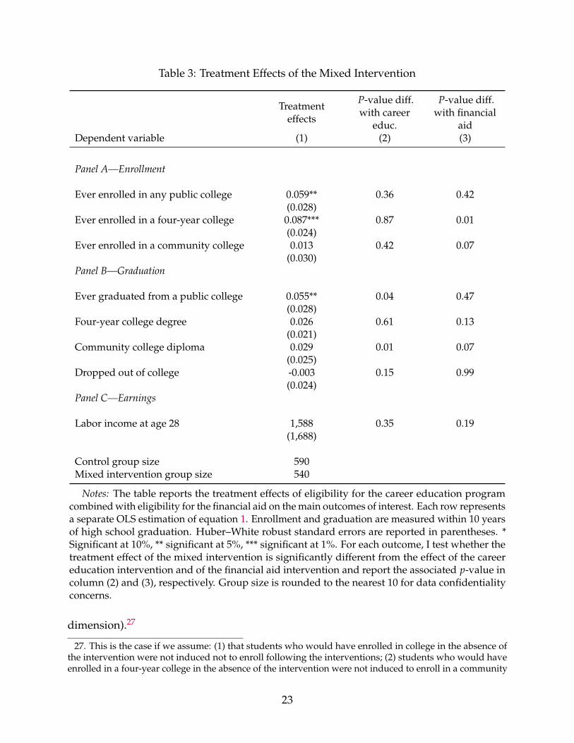
Table 3: Treatment Effects of the Mixed Intervention
Treatmenteffects
P-value diff.with career
educ.
P-value diff.with financial
aidDependent variable (1) (2) (3)
Panel A—Enrollment
Ever enrolled in any public college 0.059** 0.36 0.42(0.028)
Ever enrolled in a four-year college 0.087*** 0.87 0.01(0.024)
Ever enrolled in a community college 0.013 0.42 0.07(0.030)
Panel B—Graduation
Ever graduated from a public college 0.055** 0.04 0.47(0.028)
Four-year college degree 0.026 0.61 0.13(0.021)
Community college diploma 0.029 0.01 0.07(0.025)
Dropped out of college -0.003 0.15 0.99(0.024)
Panel C—Earnings
Labor income at age 28 1,588 0.35 0.19(1,688)
Control group size 590Mixed intervention group size 540
Notes: The table reports the treatment effects of eligibility for the career education programcombined with eligibility for the financial aid on the main outcomes of interest. Each row representsa separate OLS estimation of equation 1. Enrollment and graduation are measured within 10 yearsof high school graduation. Huber–White robust standard errors are reported in parentheses. *Significant at 10%, ** significant at 5%, *** significant at 1%. For each outcome, I test whether thetreatment effect of the mixed intervention is significantly different from the effect of the careereducation intervention and of the financial aid intervention and report the associated p-value incolumn (2) and (3), respectively. Group size is rounded to the nearest 10 for data confidentialityconcerns.
dimension).27
27. This is the case if we assume: (1) that students who would have enrolled in college in the absence ofthe intervention were not induced not to enroll following the interventions; (2) students who would haveenrolled in a four-year college in the absence of the intervention were not induced to enroll in a community
23
Consistent with these effects on enrollment, students assigned to the mixed interven-tion group were more likely to graduate from any college and from four-year college thancontrol group counterparts (+5.5 and +2.6 percentage points, respectively). The interven-tion also increased, as the career education intervention, four-year college dropout (TableA17). However, this increase is compensated by a rise in community college graduation.All in all, there was no change in the fraction of students who dropped out of college.28
Considering these findings, the effects of mixed intervention on earnings would beexpected to be similar to those of the career education intervention. Indeed, the onlydifference observed between the effects of the career education intervention and of themixed intervention is that unlike the former, the latter prompted some students to enrollin community college. However, the community college programs in which studentswere induced to enroll did not seem to yield any monetary returns. Consistent with theprediction, I observe a rise in annual labor income following the mixed intervention whichis not statistically different from the effects of the career education intervention—althoughit is smaller and not significantly different from zero.29
4.3 Effects of the Career Education Intervention on High-Income Stu-
dents’ Outcomes
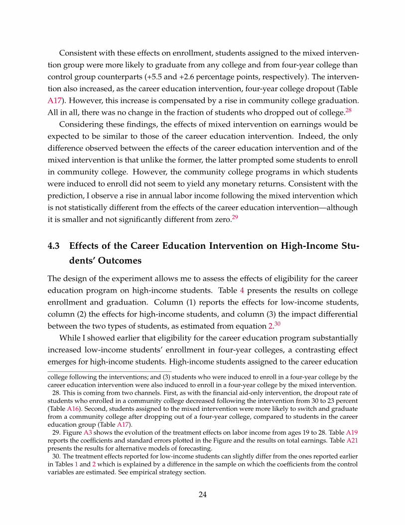
The design of the experiment allows me to assess the effects of eligibility for the careereducation program on high-income students. Table 4 presents the results on collegeenrollment and graduation. Column (1) reports the effects for low-income students,column (2) the effects for high-income students, and column (3) the impact differentialbetween the two types of students, as estimated from equation 2.30
While I showed earlier that eligibility for the career education program substantiallyincreased low-income students’ enrollment in four-year colleges, a contrasting effectemerges for high-income students. High-income students assigned to the career education
college following the interventions; and (3) students who were induced to enroll in a four-year college by thecareer education intervention were also induced to enroll in a four-year college by the mixed intervention.
28. This is coming from two channels. First, as with the financial aid-only intervention, the dropout rate ofstudents who enrolled in a community college decreased following the intervention from 30 to 23 percent(Table A16). Second, students assigned to the mixed intervention were more likely to switch and graduatefrom a community college after dropping out of a four-year college, compared to students in the careereducation group (Table A17).
29. Figure A3 shows the evolution of the treatment effects on labor income from ages 19 to 28. Table A19reports the coefficients and standard errors plotted in the Figure and the results on total earnings. Table A21presents the results for alternative models of forecasting.
30. The treatment effects reported for low-income students can slightly differ from the ones reported earlierin Tables 1 and 2 which is explained by a difference in the sample on which the coefficients from the controlvariables are estimated. See empirical strategy section.
24
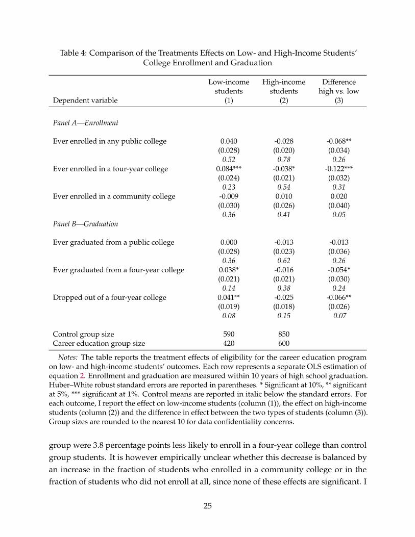
Table 4: Comparison of the Treatments Effects on Low- and High-Income Students’College Enrollment and Graduation
Low-incomestudents
High-incomestudents
Differencehigh vs. low
Dependent variable (1) (2) (3)
Panel A—Enrollment
Ever enrolled in any public college 0.040 -0.028 -0.068**(0.028) (0.020) (0.034)
0.52 0.78 0.26Ever enrolled in a four-year college 0.084*** -0.038* -0.122***
(0.024) (0.021) (0.032)0.23 0.54 0.31
Ever enrolled in a community college -0.009 0.010 0.020(0.030) (0.026) (0.040)
0.36 0.41 0.05Panel B—Graduation
Ever graduated from a public college 0.000 -0.013 -0.013(0.028) (0.023) (0.036)
0.36 0.62 0.26Ever graduated from a four-year college 0.038* -0.016 -0.054*
(0.021) (0.021) (0.030)0.14 0.38 0.24
Dropped out of a four-year college 0.041** -0.025 -0.066**(0.019) (0.018) (0.026)
0.08 0.15 0.07
Control group size 590 850Career education group size 420 600
Notes: The table reports the treatment effects of eligibility for the career education programon low- and high-income students’ outcomes. Each row represents a separate OLS estimation ofequation 2. Enrollment and graduation are measured within 10 years of high school graduation.Huber–White robust standard errors are reported in parentheses. * Significant at 10%, ** significantat 5%, *** significant at 1%. Control means are reported in italic below the standard errors. Foreach outcome, I report the effect on low-income students (column (1)), the effect on high-incomestudents (column (2)) and the difference in effect between the two types of students (column (3)).Group sizes are rounded to the nearest 10 for data confidentiality concerns.
group were 3.8 percentage points less likely to enroll in a four-year college than controlgroup students. It is however empirically unclear whether this decrease is balanced byan increase in the fraction of students who enrolled in a community college or in thefraction of students who did not enroll at all, since none of these effects are significant. I
25
also observe a reduction in the fraction of students who dropped out of four-year collegefollowing the intervention, although the effect is not statistically significant (p-value=0.16).It suggests that students who were induced not to enroll in a four-year college by theintervention would not have graduated in the absence of the intervention. Note that theeffects on high-income students do not survive multiple hypothesis testing and shouldaccordingly be taken with caution.
In next explore in Figure 3 the effects of the career education intervention on uncon-ditional labor income from ages 19 to 28. Each point is estimated from equation 2, andthe shaded area indicates the associated 90 percent confidence interval. The effects of thecareer education intervention on low-income students are presented in Panel (a) and theeffects on high-income students in Panel (b). I also report in Table A23 the correspondingcoefficients and standard errors together with the effects on total earnings.
(a) Treatment effects on low-incomestudents
−4,000
−2,000
0
2,000
4,000
6,000
8,000
19 20 21 22 23 24 25 26 27 28Age
Trea
tmen
t eff
ects
on
labo
r in
com
e ($
CA
)
(b) Treatment effects on high-incomestudents
−4,000
−2,000
0
2,000
4,000
6,000
8,000
19 20 21 22 23 24 25 26 27 28Age
Trea
tmen
t eff
ects
on
labo
r in
com
e ($
CA
)
Figure 3: Impact on Labor Income Over Time
Notes: The figure plots the effects of eligibility for the career education program on labor incomeagainst age, for both low- and high-income students. Point estimates together with the associated90 percent confidence intervals are reported. Each point is estimated from a OLS regression ofthe outcome on the treatment dummy, the treatment dummy interacted with the parental incomedummy, the parental income dummy and controls for student baseline characteristics listed in TableA3. Huber–White robust standard errors are used to compute the confidence intervals. Earningsare expressed in 2020 Canadian dollars.
Eligibility for the career education program did not have any noticeable impact onlabor income between the ages of 19 and 24. Nevertheless, starting from age 25, I observe a
26
growing positive difference in labor income between treated and control students althoughnone of these differences are statistically significant. The effects are, however, substantialand at the margin of significance—high-income students assigned to the career educationgroup earned, on average, $2,558 more annually in labor income by age 28 than controlgroup students (p-value=0.12). As with low-income students, the increase in earnings doesnot come from an increase in the likelihood of working but rather by an increase in wages(Table A20). The treatment effects are found to be similar on total earnings.
The increase in earnings is consistent with the decline in four-year college dropout. Itcan also be driven by a change in students’ major choices or the quality of the collegesthey enrolled in. I however do not find evidence that the intervention changed thesedimensions of enrollment even though I cannot rule out some small effects (Table A24).31
Together, these findings are consistent with a model where students lack informationand rely on default options (French and Oreopoulos (2017)). For instance, some low-income students might not enroll in four-year colleges because of a lack of attention andinformation on opportunities. Inversely, some high-income students with low skills andtaste for schooling might enroll in four-year colleges because that is the norm among theirpeers.
4.4 Impact on the Gaps in College Enrollment and Graduation Between
High- and Low-income Students
By expanding low-income students’ enrollment and graduation rates, the three interven-tions had sizable effects on the gaps in college enrollment and graduation between high-and low-income students—effects that are reinforced by the lower enrollment rates ofhigh-income students assigned to the career education group. In this section, I evaluatethe magnitude of the reduction in these gaps. I focus on the four-year college enrollmentand graduation gaps since my previous findings have proven little monetary benefits ofcommunity college enrollment/graduation for the marginal students.
In particular, I am interested in the gaps in enrollment and graduation between stu-dents with similar academic achievement prior to treatment. To this end, I estimate therelationship between enrollment/graduation and student test scores in Grade 9, for eachincome group and treatment arm.32 Results are illustrated in Figure 4 and Table A25
31. I do observe, conditional on enrollment, a small increase in the fraction of college students who enrolledin a STEM program. However, I do not observe a change in the overall fraction of students who enrolledin a four-year college program. It might be the case that students who were induced not to enroll in afour-year college following the intervention would not have enrolled in a STEM program in the absence ofthe intervention.
32. I standardize students test scores in each school and estimate the relationship using a polynomial
27
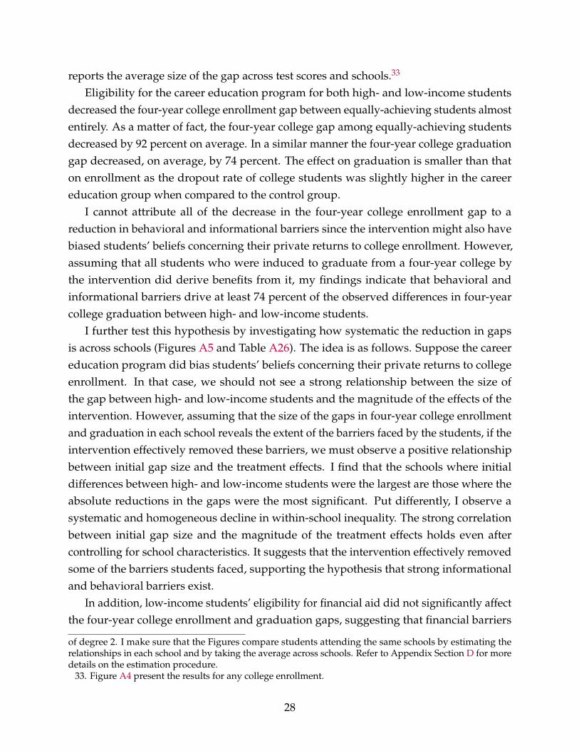
reports the average size of the gap across test scores and schools.33
Eligibility for the career education program for both high- and low-income studentsdecreased the four-year college enrollment gap between equally-achieving students almostentirely. As a matter of fact, the four-year college gap among equally-achieving studentsdecreased by 92 percent on average. In a similar manner the four-year college graduationgap decreased, on average, by 74 percent. The effect on graduation is smaller than thaton enrollment as the dropout rate of college students was slightly higher in the careereducation group when compared to the control group.
I cannot attribute all of the decrease in the four-year college enrollment gap to areduction in behavioral and informational barriers since the intervention might also havebiased students’ beliefs concerning their private returns to college enrollment. However,assuming that all students who were induced to graduate from a four-year college bythe intervention did derive benefits from it, my findings indicate that behavioral andinformational barriers drive at least 74 percent of the observed differences in four-yearcollege graduation between high- and low-income students.
I further test this hypothesis by investigating how systematic the reduction in gapsis across schools (Figures A5 and Table A26). The idea is as follows. Suppose the careereducation program did bias students’ beliefs concerning their private returns to collegeenrollment. In that case, we should not see a strong relationship between the size ofthe gap between high- and low-income students and the magnitude of the effects of theintervention. However, assuming that the size of the gaps in four-year college enrollmentand graduation in each school reveals the extent of the barriers faced by the students, if theintervention effectively removed these barriers, we must observe a positive relationshipbetween initial gap size and the treatment effects. I find that the schools where initialdifferences between high- and low-income students were the largest are those where theabsolute reductions in the gaps were the most significant. Put differently, I observe asystematic and homogeneous decline in within-school inequality. The strong correlationbetween initial gap size and the magnitude of the treatment effects holds even aftercontrolling for school characteristics. It suggests that the intervention effectively removedsome of the barriers students faced, supporting the hypothesis that strong informationaland behavioral barriers exist.
In addition, low-income students’ eligibility for financial aid did not significantly affectthe four-year college enrollment and graduation gaps, suggesting that financial barriers
of degree 2. I make sure that the Figures compare students attending the same schools by estimating therelationships in each school and by taking the average across schools. Refer to Appendix Section D for moredetails on the estimation procedure.
33. Figure A4 present the results for any college enrollment.
28
Panel A—Career education intervention
Four-year college enrollment gap
0.0
0.2
0.4
0.6
0.8
1.0
0 20 40 60 80 100Within−school percentile rank
Avg
. enr
ollm
ent r
ate
Panel B—Financial aid intervention
Four-year college enrollment gap
0.0
0.2
0.4
0.6
0.8
1.0
0 20 40 60 80 100Within−school percentile rank
Avg
. enr
ollm
ent r
ate
Four-year college graduation gap
0.0
0.2
0.4
0.6
0.8
1.0
0 20 40 60 80 100Within−school percentile rank
Avg
. gra
dua
tion
rat
e
Legend
Control x LI
Control x HI
Career educ. x LI
Career educ. x HI
Four-year college graduation gap
0.0
0.2
0.4
0.6
0.8
1.0
0 20 40 60 80 100Within−school percentile rank
Avg
. gra
dua
tion
rat
e
Legend
Control x LI
Control x HI
Financial aid x LI
Figure 4: Enrollment Rates of High- and Low-Income Studentsby Percentile Rank and Treatment Arms
Notes: The figure plots, across within-school test scores percentile rank, the four-year collegeenrollment and graduation rates of high- and low-income students. Panel A plots the rates forstudents in the career education group and Panel B the rates for students in the financial aid group.The enrollment rates in the control group are also shown for comparability purposes. Each rate is asimple average of the rates across the 30 schools, as estimated from equation A5.
do not play a major role in the four-year college enrollment and graduation gaps.Overall, these findings indicate that career education is an important tool for aligning
29
the four-year college enrollment and graduation rates of high- and low-income studentswith similar academic achievement. However, while the intervention effectively reducedinequality among equally-achieving pupils, differences in academic achievement accountfor a large part of the observed differences in enrollment and graduation between high-and low-income students (56–63 percent, Table A27). To fully decrease the gaps betweenthe two types of students, one might also understand the factors driving the differences inacademic achievement.
5 Conclusion
This paper investigates the effects of college grant aid, career education in high school, andthe combination of the two on students’ college enrollment, graduation, and earnings. Ishow that career education programs have the potential to improve students’ long-termoutcomes substantially. My results suggest that the reason why these types of programs areso effective stems from the existence of information and behavioral barriers that preventstudents from making optimal decisions regarding post-secondary education. Removingthese barriers will induce more low-income students and less high-income students toenroll in four-year colleges, resulting in a sharp reduction in the enrollment and graduationgaps between the two types of students.
One limitation of my study is the lack of power, which prevents any clear explorationof treatment effect heterogeneity. As the career education program resulted in increase inboth graduation and dropout rates, I suspect heterogeneous benefits of the intervention onstudents. Further work should aim to understand who benefited from the intervention andwho did not. This understanding would facilitate the design of career education programsthat are better suited to helping all types of students.
Moreover, a key question remains unanswered: what features of the career educationprogram were the more effective at increasing low- income students’ enrollment? Previousstudies suggest that the provision of information alone is not helpful is increasing students’enrollment rates (Bird et al. (2021); Kerr et al. (2015); Bonilla, Bottan, and Ham (2015);Hastings et al. (2016); Carrell and Sacerdote (2017)). By contrast, the intervention providedinsights into the post-secondary education application process and decision-making, adimension that has proven to be effective in increasing college enrollment rates (Avery(2013); Stephan and Rosenbaum (2013); Castleman, Page, and Schooley (2014); Carrelland Sacerdote (2017); Cunha, Miller, and Weisburst (2018); Oreopoulos and Ford (2019)).The fact that programs offering guidance are so efficacious in increasing the enrollment ofstudents and (as I show) in enhancing their long-term outcomes is likely to be explained
30
by their lack of attention when it comes to college possibilities (French and Oreopoulos(2017)).
In this paper, I also show that providing students with additional financial aid hasno monetary benefits in the long run. This result was surprising given the fact that theintervention led to an increase in the fraction of students who enrolled and graduated fromcommunity colleges. It indicates that students were induced to enroll in programs withlimited monetary returns. This lack of returns might be specific to the marginal studentsbut might also arise from a general lack of benefits of some community college programs.My findings underscore the importance of understanding the returns to community collegeattendance.
The extent to which my findings extend to other contexts and countries remains tobe seen. There are strong reasons to believe that my main finding, according to whichcareer education programs are efficacious in enhancing students’ long-term outcomes, canbe extended to other contexts as well. In fact, many US-specific studies demonstratedthat career counseling programs, as the program studied in this paper, are effective inincreasing students’ enrollment in four-year colleges. It is thus natural to think that theywould also result in an increase in earnings.
However, my results on the effects of the financial aid intervention are possibly specificto the Canadian context. Two features of the Canadian context make it different fromother countries. First, unlike other countries, Canada is characterized by a very highenrollment rate in community and private career colleges, which might make the resultson community colleges specific to this country. Second, public colleges and universitiesare highly subsidized, and a number of grants and loans are already available in Canada,making financial constraints possibly less binding than in countries with weaker financialaid systems.
In the future, I plan to pursue my analysis of the Future to Discover experiment in threeways. First, I will continue to track students to confirm my findings on the long-term effectsof the three interventions and assess their overall effects on lifetime earnings. Second, I willbuild a structural model of college enrollment under imperfect information and Bayesianlearning to exactly quantify the extent to which students are affected by informationaland behavioral barriers and provide counterfactual estimates of the gain in earnings thatremoving these barriers would create. Third, I will exploit exogenous variations in thetiming of career counseling workshops created by weather conditions in order to identifyhow the timing of information affects the decisions made by students.
31
References
Anderson, Michael L. 2008. “Multiple inference and gender differences in the effects ofearly intervention: A reevaluation of the Abecedarian, Perry Preschool, and EarlyTraining Projects.” Journal of the American Statistical Association 103 (484): 1481–1495.
Avery, Christopher. 2013. “Evaluation of the College Possible Program: Results from aRandomized Controlled Trial.”
Bailey, Drew H., Greg J. Duncan, Flávio Cunha, Barbara R. Foorman, and David S. Yeager.2020. “Persistence and Fade-Out of Educational-Intervention Effects: Mechanisms andPotential Solutions.” Psychological Science in the Public Interest 21 (2): 55–97.
Bailey, Martha, and Susan Dynarski. 2011. “Gains and Gaps: Changing Inequality in U.S.College Entry and Completion.”
Becker, Gary S. 1964. Human Capital: A Theoretical and Empirical Analysis, with SpecialReference to Education.
Belley, Philippe, Marc Frenette, and Lance J. Lochner. 2014. “Post-secondary attendanceby parental income in the U.S. and Canada: Do financial aid policies explain thedifferences?” Canadian Journal of Economics/Revue canadienne d’économique 47 (2): 664–696.
Belley, Philippe, and Lance J. Lochner. 2007. “The Changing Role of Family Income andAbility in Determining Educational Achievement.” Journal of Human Capital 1 (1):37–89.
Belloni, Alexandre, Victor Chernozhukov, and Christian Hansen. 2013. “Inference ontreatment effects after selection among high-dimensional controls.” Review of EconomicStudies 81 (2): 608–650.
Benjamini, Yoav, Abba M Krieger, and Daniel Yekutieli. 2006. “Adaptive linear step-upprocedures that control the false discovery rate.” Biometrika 93 (3): 491–507.
Bettinger, Eric P., Oded Gurantz, Laura Kawano, Bruce Sacerdote, and Michael Stevens.2019. “The long-run impacts of financial aid: Evidence from California’s Cal Grant.”American Economic Journal: Economic Policy 11 (1): 64–94.
32
Bettinger, Eric P., Bridget Terry Long, Philip Oreopoulos, and Lisa Sanbonmatsu. 2012.“The role of application assistance and information in college decisions: Results fromthe H&R Bock FASFA experiment.” Quarterly Journal of Economics 127 (3): 1205–1242.
Bird, Kelli A., Benjamin L. Castleman, Jeffrey T. Denning, Joshua Goodman, Cait Lam-berton, and Kelly Ochs Rosinger. 2021. “Nudging at scale: Experimental evidencefrom FAFSA completion campaigns.” Journal of Economic Behavior and Organization183:105–128.
Blossfeld, Hans-Peter, and Yossi Shavit. 1993. Persisting Barriers: Changes in EducationalOpportunities in Thirteen Countries, 408.
Bonilla, Leonardo, Nicolas L Bottan, and Andrés Ham. 2015. “Information Policies andHigher Education Choices: Experimental Evidence from Colombia.”
Carrell, Scott, and Bruce Sacerdote. 2017. “Why do college-going interventions work?”American Economic Journal: Applied Economics 9 (3): 124–151.
Castleman, Benjamin L., and Joshua Goodman. 2018. “Intensive College Counseling andthe Enrollment and Persistence of Low-Income Students.” Education Finance and Policy13 (1): 19–41.
Castleman, Benjamin L., and Bridget Terry Long. 2016. “Looking beyond enrollment: Thecausal effect of need-based grants on college access, persistence, and graduation.”Journal of Labor Economics 34 (4): 1023–1073.
Castleman, Benjamin L., Lindsay C. Page, and Korynn Schooley. 2014. “The ForgottenSummer: Does the Offer of College Counseling After High School Mitigate SummerMelt Among College-Intending, Low-Income High School Graduates?” Journal ofPolicy Analysis and Management 33 (2): 320–344.
Chetty, Raj, Nathaniel Hendren, Patrick Kline, Emmanuel Saez, and Nicholas Turner. 2014.“Is the United States still a land of opportunity? Recent trends in intergenerationalmobility.” American Economic Review 104 (5): 141–147.
Cunha, Jesse M., Trey Miller, and Emily Weisburst. 2018. “Information and College Deci-sions: Evidence From the Texas GO Center Project.” Educational Evaluation and PolicyAnalysis 40 (1): 151–170.
Currie, Sheila, Judith Hutchison, Reuben Ford, Isaac Kwakye, and Doug Tattrie. 2007.Future to Discover: Early Implementation Report. Technical report.
33
Denning, Jeffrey T., Benjamin M. Marx, and Lesley J. Turner. 2019. “ProPelled: The effectsof grants on graduation, earnings, and welfare.” American Economic Journal: AppliedEconomics 11 (3): 193–224.
Dynarski, Susan, C. Libassi, Katherine Michelmore, and Stephanie Owen. 2021. “Closingthe Gap: The Effect of Reducing Complexity and Uncertainty in College Pricing onthe Choices of Low-Income Students.” American Economic Review 111 (6): 1721–56.
Eng, Amanda, and Jordan Matsudaira. 2021. “Pell grants and student success: Evidencefrom the universe of federal aid recipients.” Journal of Labor Economics 39 (S2): S413–S454.
Fack, Gabrielle, and Julien Grenet. 2015. “Improving college access and success for low-income students: Evidence from a large need-based grant program.” American Eco-nomic Journal: Applied Economics 7 (2): 1–34.
Ford, Reuben, Marc Frenette, Claudia Nicholson, Isaac Kwakye, Taylor S. Hui, JudithHutchison, Sabina Dobrer, Heather S. Fowler, and Shopie Hébert. 2012. Future toDiscover: Post-secondary Impacts Report. Technical report.
Ford, Reuben, and Isaac Kwakye. 2016. Future to Discover: Sixth Year Post-secondary ImpactsReport. Technical report. Social Research and Demonstration Corporation.
French, Robert, and Philip Oreopoulos. 2017. “Behavioral barriers transitioning to college.”Labour Economics 47:48–63.
Frenette, Marc. 2017. Postsecondary Enrolment by Parental Income : Recent National andProvincial Trends. Technical report Economic insights, no. 70. Statistics Canada.
Goldrick-Rab, Sara, Robert Kelchen, Douglas N Harris, and James Benson. 2016. “Reducingincome inequality in educational attainment: Experimental evidence on the impact offinancial aid on college completion.” American Journal of Sociology 121 (6): 1762–1817.
Hastings, Justine S., Christopher A. Neilson, Anely Ramirez, and Seth D. Zimmerman.2016. “(Un)informed college and major choice: Evidence from linked survey andadministrative data.” Economics of Education Review 51:136–151.
Herbaut, Estelle, and Koen Geven. 2020. “What works to reduce inequalities in highereducation? A systematic review of the (quasi-)experimental literature on outreach andfinancial aid.” Research in Social Stratification and Mobility 65.
34
Heß, Simon. 2017. “Randomization inference with stata: A guide and software.” StataJournal 17 (3): 630–651.
Hoxby, Caroline M., and Christopher Avery. 2013. “The Missing "One-Offs": The HiddenSupply of High-Achieving, Low Income Students.” Brookings Papers on EconomicActivity 2013 (1): 1–65.
Hui, Taylor S., and Reuben Ford. 2018. Education and Labour Market Impacts of the Future toDiscover Project: Summary of Key Findings. Technical report. Toronto: Higher EducationQuality Council of Ontario.
Jones, Glen A., and Sharon X. Li. 2015. “The “Invisible” Sector: Private Higher Educationin Canada.” In Private Higher Education: A Global Perspective, 1–33.
Keane, Michael P., and Kenneth I. Wolpin. 2001. “The Effect of Parental Transfers andBorrowing Constraints on Educational Attainment.” International Economic Review 42(4): 1051–1103.
Kerr, Sari Pekkala, Tuomas Pekkarinen, Matti Sarvimäki, and Roope Uusitalo. 2015. “Post-Secondary Education and Information on Labor Market Prospects: A RandomizedField Experiment.”
Kinsler, Josh, and Ronni Pavan. 2011. “Family income and higher education choices: Theimportance of accounting for college quality.” Journal of Human Capital 5 (4): 453–477.
Lochner, Lance J., and Alexander Monge-Naranjo. 2012. “Credit Constraints in Education.”Annual Review of Economics 4 (1): 225–256.
Oreopoulos, Philip, and Reuben Ford. 2019. “Keeping College Options Open: A FieldExperiment to Help all High School Seniors Through the College Application Process.”Journal of Policy Analysis and Management 38 (2): 426–454.
Oreopoulos, Philip, and Kjell G. Salvanes. 2011. “Priceless: The nonpecuniary benefits ofschooling.” Journal of Economic Perspectives 25 (1): 159–184.
Page, Lindsay C., and Judith Scott-Clayton. 2016. “Improving college access in the UnitedStates: Barriers and policy responses.” Economics of Education Review 51:4–22.
Scott-Clayton, Judith, and Basit Zafar. 2019. “Financial aid, debt management, and socioe-conomic outcomes: Post-college effects of merit-based aid.” Journal of Public Economics170:68–82.
35
Seaman, Shaun R, and Ian R White. 2013. “Review of inverse probability weighting fordealing with missing data.” Statistical Methods in Medical Research 22 (3): 278–295.
Statistics Canada. 2020. Education Indicators in Canada: An International Perspective 2020.Technical report.
Stephan, Jennifer L, and James E Rosenbaum. 2013. “Can High Schools Reduce CollegeEnrollment Gaps With a New Counseling Model?” Educational Evaluation and PolicyAnalysis 35 (2): 200–219.
Wooldridge, Jeffrey M. 2010. Econometric Analysis of Cross Section and Panel Data. MIT press.
Young, Alwyn. 2019. “Channeling Fisher: Randomization tests and the statistical insignifi-cance of seemingly significant experimental results.” Quarterly Journal of Economics134 (2): 557–598.
36
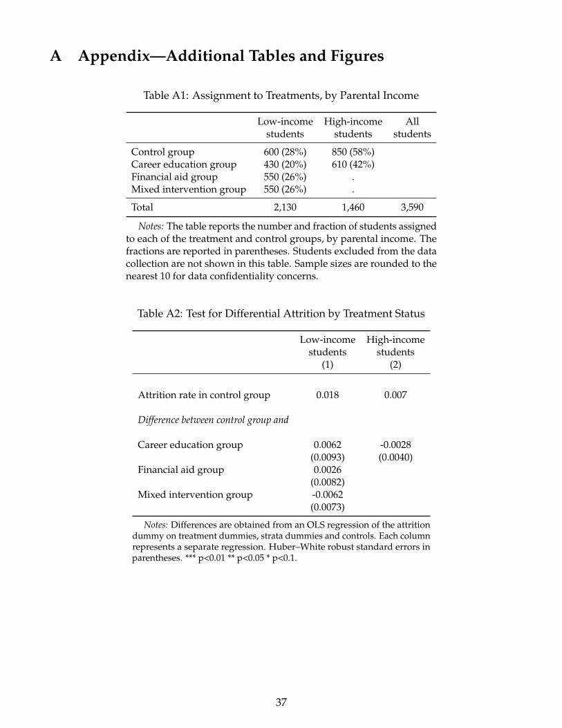
A Appendix—Additional Tables and Figures
Table A1: Assignment to Treatments, by Parental Income
Low-income High-income Allstudents students students
Control group 600 (28%) 850 (58%)Career education group 430 (20%) 610 (42%)Financial aid group 550 (26%) .Mixed intervention group 550 (26%) .
Total 2,130 1,460 3,590
Notes: The table reports the number and fraction of students assignedto each of the treatment and control groups, by parental income. Thefractions are reported in parentheses. Students excluded from the datacollection are not shown in this table. Sample sizes are rounded to thenearest 10 for data confidentiality concerns.
Table A2: Test for Differential Attrition by Treatment Status
Low-income High-incomestudents students
(1) (2)
Attrition rate in control group 0.018 0.007
Difference between control group and
Career education group 0.0062 -0.0028(0.0093) (0.0040)
Financial aid group 0.0026(0.0082)
Mixed intervention group -0.0062(0.0073)
Notes: Differences are obtained from an OLS regression of the attritiondummy on treatment dummies, strata dummies and controls. Each columnrepresents a separate regression. Huber–White robust standard errors inparentheses. *** p<0.01 ** p<0.05 * p<0.1.
37
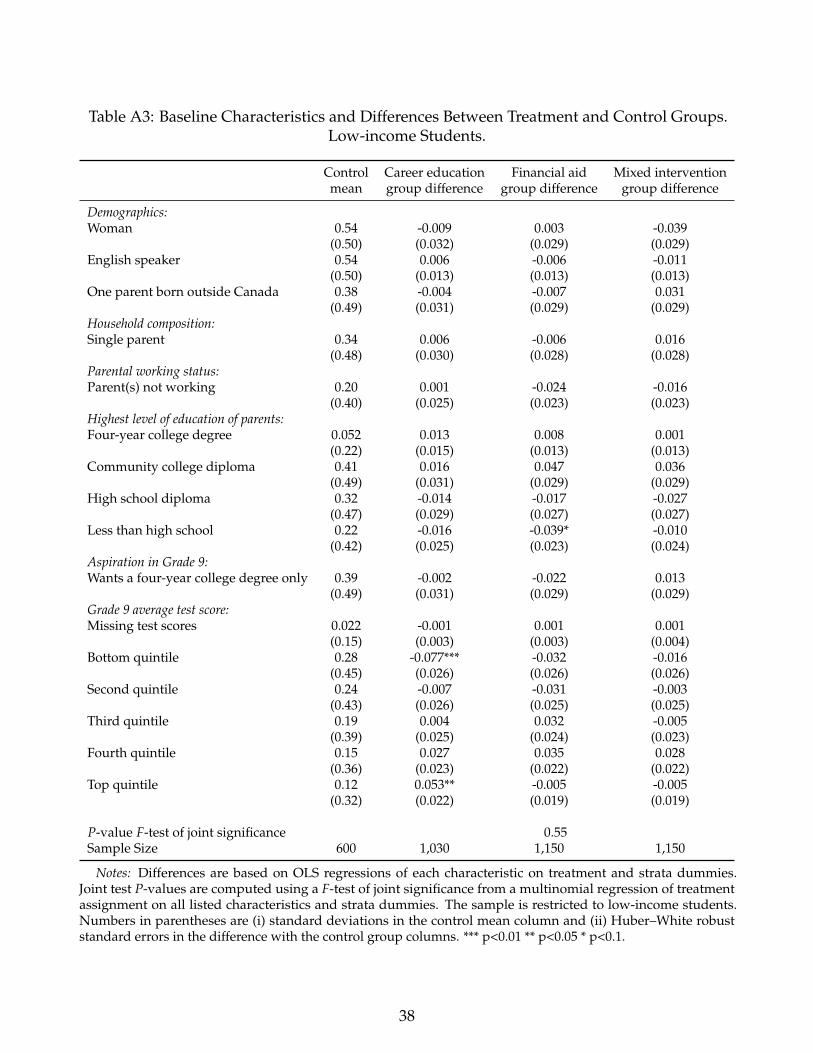
Table A3: Baseline Characteristics and Differences Between Treatment and Control Groups.Low-income Students.
Control Career education Financial aid Mixed interventionmean group difference group difference group difference
Demographics:Woman 0.54 -0.009 0.003 -0.039
(0.50) (0.032) (0.029) (0.029)English speaker 0.54 0.006 -0.006 -0.011
(0.50) (0.013) (0.013) (0.013)One parent born outside Canada 0.38 -0.004 -0.007 0.031
(0.49) (0.031) (0.029) (0.029)Household composition:Single parent 0.34 0.006 -0.006 0.016
(0.48) (0.030) (0.028) (0.028)Parental working status:Parent(s) not working 0.20 0.001 -0.024 -0.016
(0.40) (0.025) (0.023) (0.023)Highest level of education of parents:Four-year college degree 0.052 0.013 0.008 0.001
(0.22) (0.015) (0.013) (0.013)Community college diploma 0.41 0.016 0.047 0.036
(0.49) (0.031) (0.029) (0.029)High school diploma 0.32 -0.014 -0.017 -0.027
(0.47) (0.029) (0.027) (0.027)Less than high school 0.22 -0.016 -0.039* -0.010
(0.42) (0.025) (0.023) (0.024)Aspiration in Grade 9:Wants a four-year college degree only 0.39 -0.002 -0.022 0.013
(0.49) (0.031) (0.029) (0.029)Grade 9 average test score:Missing test scores 0.022 -0.001 0.001 0.001
(0.15) (0.003) (0.003) (0.004)Bottom quintile 0.28 -0.077*** -0.032 -0.016
(0.45) (0.026) (0.026) (0.026)Second quintile 0.24 -0.007 -0.031 -0.003
(0.43) (0.026) (0.025) (0.025)Third quintile 0.19 0.004 0.032 -0.005
(0.39) (0.025) (0.024) (0.023)Fourth quintile 0.15 0.027 0.035 0.028
(0.36) (0.023) (0.022) (0.022)Top quintile 0.12 0.053** -0.005 -0.005
(0.32) (0.022) (0.019) (0.019)
P-value F-test of joint significance 0.55Sample Size 600 1,030 1,150 1,150
Notes: Differences are based on OLS regressions of each characteristic on treatment and strata dummies.Joint test P-values are computed using a F-test of joint significance from a multinomial regression of treatmentassignment on all listed characteristics and strata dummies. The sample is restricted to low-income students.Numbers in parentheses are (i) standard deviations in the control mean column and (ii) Huber–White robuststandard errors in the difference with the control group columns. *** p<0.01 ** p<0.05 * p<0.1.
38
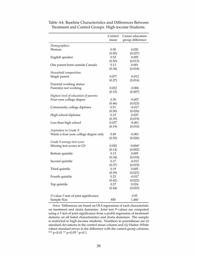
Table A4: Baseline Characteristics and Differences BetweenTreatment and Control Groups. High-income Students.
Control Career educationmean group difference
Demographics:Woman 0.50 0.020
(0.50) (0.027)English speaker 0.52 0.005
(0.50) (0.013)One parent born outside Canada 0.13 0.001
(0.34) (0.018)Household composition:Single parent 0.077 -0.012
(0.27) (0.014)Parental working status:Parent(s) not working 0.022 -0.006
(0.15) (0.007)Highest level of education of parents:Four-year college degree 0.30 -0.007
(0.46) (0.023)Community college diploma 0.51 -0.017
(0.50) (0.026)High school diploma 0.15 0.025
(0.35) (0.019)Less than high school 0.037 -0.001
(0.19) (0.010)Aspiration in Grade 9:Wants a four-year college degree only 0.49 -0.001
(0.50) (0.026)Grade 9 average test score:Missing test scores in G9 0.020 -0.004*
(0.14) (0.002)Bottom quintile 0.13 0.005
(0.34) (0.018)Second quintile 0.17 -0.012
(0.37) (0.019)Third quintile 0.19 0.005
(0.39) (0.021)Fourth quintile 0.23 -0.017
(0.42) (0.022)Top quintile 0.27 0.024
(0.44) (0.023)
P-value F-test of joint significance 0.95Sample Size 850 1,460
Notes: Differences are based on OLS regressions of each characteristicon treatment and strata dummies. Joint test P-values are computedusing a F-test of joint significance from a probit regression of treatmentdummy on all listed characteristics and strata dummies. The sampleis restricted to high-income students. Numbers in parentheses are (i)standard deviations in the control mean column and (ii) Huber–Whiterobust standard errors in the difference with the control group columns.*** p<0.01 ** p<0.05 * p<0.1.
39
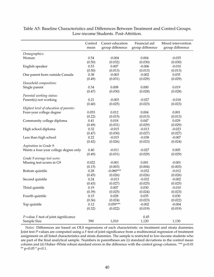
Table A5: Baseline Characteristics and Differences Between Treatment and Control Groups.Low-income Students. Post-Attrition.
Control Career education Financial aid Mixed interventionmean group difference group difference group difference
Demographics:Woman 0.54 -0.004 0.004 -0.035
(0.50) (0.032) (0.030) (0.030)English speaker 0.53 0.007 -0.006 -0.010
(0.50) (0.013) (0.013) (0.013)One parent born outside Canada 0.38 -0.003 -0.002 0.035
(0.49) (0.031) (0.029) (0.029)Household composition:Single parent 0.34 0.008 0.000 0.019
(0.47) (0.030) (0.028) (0.028)Parental working status:Parent(s) not working 0.21 -0.003 -0.027 -0.018
(0.40) (0.025) (0.023) (0.023)Highest level of education of parents:Four-year college degree 0.053 0.012 0.004 0.001
(0.22) (0.015) (0.013) (0.013)Community college diploma 0.41 0.018 0.047 0.029
(0.49) (0.031) (0.029) (0.029)High school diploma 0.32 -0.015 -0.013 -0.023
(0.47) (0.030) (0.027) (0.027)Less than high school 0.22 -0.015 -0.038 -0.007
(0.42) (0.026) (0.023) (0.024)Aspiration in Grade 9:Wants a four-year college degree only 0.40 -0.011 -0.027 0.005
(0.49) (0.031) (0.029) (0.029)Grade 9 average test score:Missing test scores in G9 0.022 -0.001 0.001 -0.001
(0.15) (0.003) (0.004) (0.003)Bottom quintile 0.28 -0.080*** -0.032 -0.012
(0.45) (0.026) (0.026) (0.026)Second quintile 0.24 -0.013 -0.032 -0.002
(0.43) (0.027) (0.025) (0.025)Third quintile 0.19 0.007 0.030 -0.010
(0.39) (0.025) (0.024) (0.023)Fourth quintile 0.15 0.028 0.035 0.030
(0.36) (0.024) (0.023) (0.022)Top quintile 0.12 0.059*** -0.002 -0.004
(0.32) (0.022) (0.019) (0.019)
P-value F-test of joint significance 0.45Sample Size 590 1,010 1,120 1,130
Notes: Differences are based on OLS regressions of each characteristic on treatment and strata dummies.Joint test P-values are computed using a F-test of joint significance from a multinomial regression of treatmentassignment on all listed characteristics and strata dummies. The sample is restricted to low-income students whoare part of the final analytical sample. Numbers in parentheses are (i) standard deviations in the control meancolumn and (ii) Huber–White robust standard errors in the difference with the control group columns. *** p<0.01** p<0.05 * p<0.1.
40
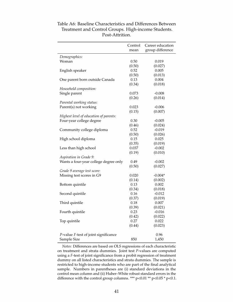
Table A6: Baseline Characteristics and Differences BetweenTreatment and Control Groups. High-income Students.
Post-Attrition.
Control Career educationmean group difference
Demographics:Woman 0.50 0.019
(0.50) (0.027)English speaker 0.52 0.005
(0.50) (0.013)One parent born outside Canada 0.13 0.004
(0.34) (0.018)Household composition:Single parent 0.073 -0.008
(0.26) (0.014)Parental working status:Parent(s) not working 0.023 -0.006
(0.15) (0.007)Highest level of education of parents:Four-year college degree 0.30 -0.005
(0.46) (0.024)Community college diploma 0.52 -0.019
(0.50) (0.026)High school diploma 0.15 0.025
(0.35) (0.019)Less than high school 0.037 -0.002
(0.19) (0.010)Aspiration in Grade 9:Wants a four-year college degree only 0.49 -0.002
(0.50) (0.027)Grade 9 average test score:Missing test scores in G9 0.020 -0.004*
(0.14) (0.002)Bottom quintile 0.13 0.002
(0.34) (0.018)Second quintile 0.16 -0.012
(0.37) (0.019)Third quintile 0.18 0.007
(0.39) (0.021)Fourth quintile 0.23 -0.016
(0.42) (0.022)Top quintile 0.27 0.022
(0.44) (0.023)
P-value F-test of joint significance 0.96Sample Size 850 1,450
Notes: Differences are based on OLS regressions of each characteristicon treatment and strata dummies. Joint test P-values are computedusing a F-test of joint significance from a probit regression of treatmentdummy on all listed characteristics and strata dummies. The sample isrestricted to high-income students who are part of the final analyticalsample. Numbers in parentheses are (i) standard deviations in thecontrol mean column and (ii) Huber–White robust standard errors in thedifference with the control group columns. *** p<0.01 ** p<0.05 * p<0.1.
41
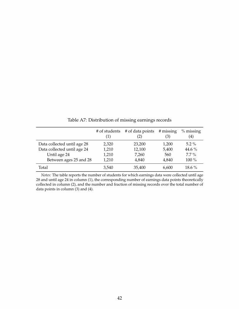
Table A7: Distribution of missing earnings records
# of students # of data points # missing % missing(1) (2) (3) (4)
Data collected until age 28 2,320 23,200 1,200 5.2 %Data collected until age 24 1,210 12,100 5,400 44.6 %
Until age 24 1,210 7,260 560 7.7 %Between ages 25 and 28 1,210 4,840 4,840 100 %
Total 3,540 35,400 6,600 18.6 %
Notes: The table reports the number of students for which earnings data were collected until age28 and until age 24 in column (1), the corresponding number of earnings data points theoreticallycollected in column (2), and the number and fraction of missing records over the total number ofdata points in column (3) and (4).
42
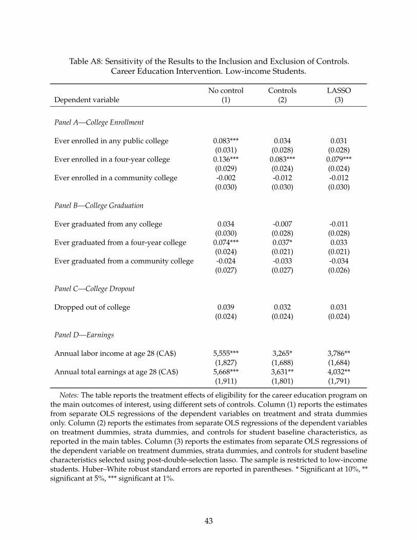
Table A8: Sensitivity of the Results to the Inclusion and Exclusion of Controls.Career Education Intervention. Low-income Students.
No control Controls LASSODependent variable (1) (2) (3)
Panel A—College Enrollment
Ever enrolled in any public college 0.083*** 0.034 0.031(0.031) (0.028) (0.028)
Ever enrolled in a four-year college 0.136*** 0.083*** 0.079***(0.029) (0.024) (0.024)
Ever enrolled in a community college -0.002 -0.012 -0.012(0.030) (0.030) (0.030)
Panel B—College Graduation
Ever graduated from any college 0.034 -0.007 -0.011(0.030) (0.028) (0.028)
Ever graduated from a four-year college 0.074*** 0.037* 0.033(0.024) (0.021) (0.021)
Ever graduated from a community college -0.024 -0.033 -0.034(0.027) (0.027) (0.026)
Panel C—College Dropout
Dropped out of college 0.039 0.032 0.031(0.024) (0.024) (0.024)
Panel D—Earnings
Annual labor income at age 28 (CA$) 5,555*** 3,265* 3,786**(1,827) (1,688) (1,684)
Annual total earnings at age 28 (CA$) 5,668*** 3,631** 4,032**(1,911) (1,801) (1,791)
Notes: The table reports the treatment effects of eligibility for the career education program onthe main outcomes of interest, using different sets of controls. Column (1) reports the estimatesfrom separate OLS regressions of the dependent variables on treatment and strata dummiesonly. Column (2) reports the estimates from separate OLS regressions of the dependent variableson treatment dummies, strata dummies, and controls for student baseline characteristics, asreported in the main tables. Column (3) reports the estimates from separate OLS regressions ofthe dependent variable on treatment dummies, strata dummies, and controls for student baselinecharacteristics selected using post-double-selection lasso. The sample is restricted to low-incomestudents. Huber–White robust standard errors are reported in parentheses. * Significant at 10%, **significant at 5%, *** significant at 1%.
43
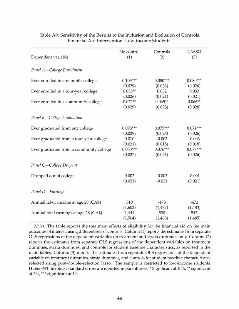
Table A9: Sensitivity of the Results to the Inclusion and Exclusion of Controls.Financial Aid Intervention. Low-income Students.
No control Controls LASSODependent variable (1) (2) (3)
Panel A—College Enrollment
Ever enrolled in any public college 0.103*** 0.080*** 0.080***(0.029) (0.026) (0.026)
Ever enrolled in a four-year college 0.053** 0.032 0.032(0.026) (0.021) (0.021)
Ever enrolled in a community college 0.072** 0.065** 0.066**(0.029) (0.028) (0.028)
Panel B—College Graduation
Ever graduated from any college 0.093*** 0.075*** 0.074***(0.029) (0.026) (0.026)
Ever graduated from a four-year college 0.010 -0.003 -0.003(0.021) (0.018) (0.018)
Ever graduated from a community college 0.083*** 0.076*** 0.077***(0.027) (0.026) (0.026)
Panel C—College Dropout
Dropped out of college 0.002 -0.003 -0.001(0.021) -0.021 (0.021)
Panel D—Earnings
Annual labor income at age 28 (CA$) 510 -473 -472(1,603) (1,477) (1,483)
Annual total earnings at age 28 (CA$) 1,441 530 545(1,564) (1,483) (1,485)
Notes: The table reports the treatment effects of eligibility for the financial aid on the mainoutcomes of interest, using different sets of controls. Column (1) reports the estimates from separateOLS regressions of the dependent variables on treatment and strata dummies only. Column (2)reports the estimates from separate OLS regressions of the dependent variables on treatmentdummies, strata dummies, and controls for student baseline characteristics, as reported in themain tables. Column (3) reports the estimates from separate OLS regressions of the dependentvariable on treatment dummies, strata dummies, and controls for student baseline characteristicsselected using post-double-selection lasso. The sample is restricted to low-income students.Huber–White robust standard errors are reported in parentheses. * Significant at 10%, ** significantat 5%, *** significant at 1%.
44
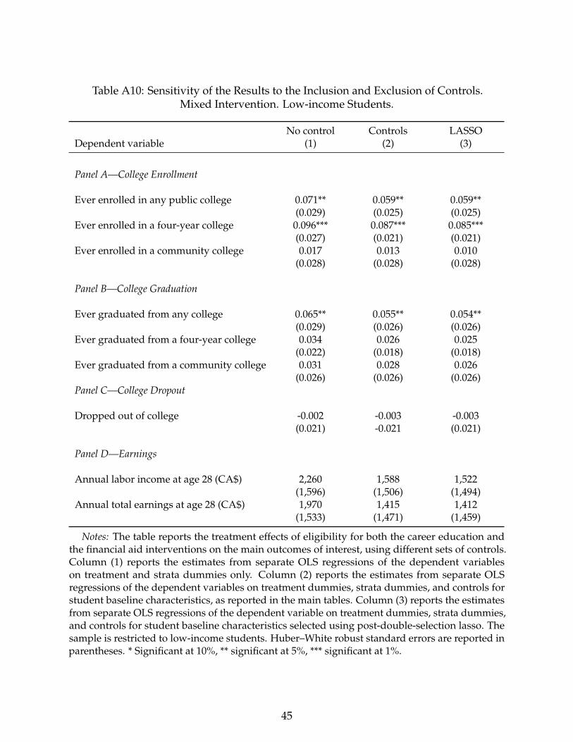
Table A10: Sensitivity of the Results to the Inclusion and Exclusion of Controls.Mixed Intervention. Low-income Students.
No control Controls LASSODependent variable (1) (2) (3)
Panel A—College Enrollment
Ever enrolled in any public college 0.071** 0.059** 0.059**(0.029) (0.025) (0.025)
Ever enrolled in a four-year college 0.096*** 0.087*** 0.085***(0.027) (0.021) (0.021)
Ever enrolled in a community college 0.017 0.013 0.010(0.028) (0.028) (0.028)
Panel B—College Graduation
Ever graduated from any college 0.065** 0.055** 0.054**(0.029) (0.026) (0.026)
Ever graduated from a four-year college 0.034 0.026 0.025(0.022) (0.018) (0.018)
Ever graduated from a community college 0.031 0.028 0.026(0.026) (0.026) (0.026)
Panel C—College Dropout
Dropped out of college -0.002 -0.003 -0.003(0.021) -0.021 (0.021)
Panel D—Earnings
Annual labor income at age 28 (CA$) 2,260 1,588 1,522(1,596) (1,506) (1,494)
Annual total earnings at age 28 (CA$) 1,970 1,415 1,412(1,533) (1,471) (1,459)
Notes: The table reports the treatment effects of eligibility for both the career education andthe financial aid interventions on the main outcomes of interest, using different sets of controls.Column (1) reports the estimates from separate OLS regressions of the dependent variableson treatment and strata dummies only. Column (2) reports the estimates from separate OLSregressions of the dependent variables on treatment dummies, strata dummies, and controls forstudent baseline characteristics, as reported in the main tables. Column (3) reports the estimatesfrom separate OLS regressions of the dependent variable on treatment dummies, strata dummies,and controls for student baseline characteristics selected using post-double-selection lasso. Thesample is restricted to low-income students. Huber–White robust standard errors are reported inparentheses. * Significant at 10%, ** significant at 5%, *** significant at 1%.
45
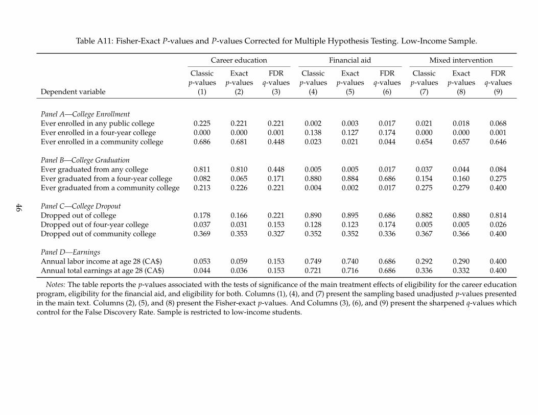
Table A11: Fisher-Exact P-values and P-values Corrected for Multiple Hypothesis Testing. Low-Income Sample.
Career education Financial aid Mixed intervention
Classicp-values
Exactp-values
FDRq-values
Classicp-values
Exactp-values
FDRq-values
Classicp-values
Exactp-values
FDRq-values
Dependent variable (1) (2) (3) (4) (5) (6) (7) (8) (9)
Panel A—College EnrollmentEver enrolled in any public college 0.225 0.221 0.221 0.002 0.003 0.017 0.021 0.018 0.068Ever enrolled in a four-year college 0.000 0.000 0.001 0.138 0.127 0.174 0.000 0.000 0.001Ever enrolled in a community college 0.686 0.681 0.448 0.023 0.021 0.044 0.654 0.657 0.646
Panel B—College GraduationEver graduated from any college 0.811 0.810 0.448 0.005 0.005 0.017 0.037 0.044 0.084Ever graduated from a four-year college 0.082 0.065 0.171 0.880 0.884 0.686 0.154 0.160 0.275Ever graduated from a community college 0.213 0.226 0.221 0.004 0.002 0.017 0.275 0.279 0.400
Panel C—College DropoutDropped out of college 0.178 0.166 0.221 0.890 0.895 0.686 0.882 0.880 0.814Dropped out of four-year college 0.037 0.031 0.153 0.128 0.123 0.174 0.005 0.005 0.026Dropped out of community college 0.369 0.353 0.327 0.352 0.352 0.336 0.367 0.366 0.400
Panel D—EarningsAnnual labor income at age 28 (CA$) 0.053 0.059 0.153 0.749 0.740 0.686 0.292 0.290 0.400Annual total earnings at age 28 (CA$) 0.044 0.036 0.153 0.721 0.716 0.686 0.336 0.332 0.400
Notes: The table reports the p-values associated with the tests of significance of the main treatment effects of eligibility for the career educationprogram, eligibility for the financial aid, and eligibility for both. Columns (1), (4), and (7) present the sampling based unadjusted p-values presentedin the main text. Columns (2), (5), and (8) present the Fisher-exact p-values. And Columns (3), (6), and (9) present the sharpened q-values whichcontrol for the False Discovery Rate. Sample is restricted to low-income students.
46
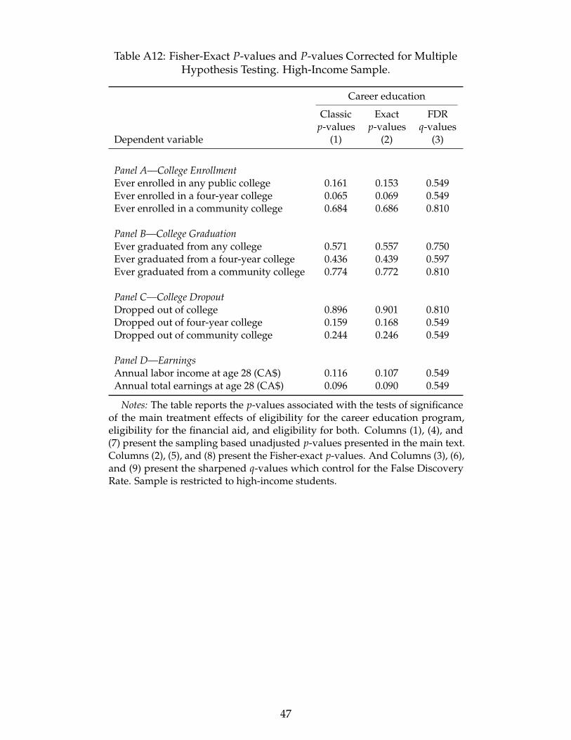
Table A12: Fisher-Exact P-values and P-values Corrected for MultipleHypothesis Testing. High-Income Sample.
Career education
Classicp-values
Exactp-values
FDRq-values
Dependent variable (1) (2) (3)
Panel A—College EnrollmentEver enrolled in any public college 0.161 0.153 0.549Ever enrolled in a four-year college 0.065 0.069 0.549Ever enrolled in a community college 0.684 0.686 0.810
Panel B—College GraduationEver graduated from any college 0.571 0.557 0.750Ever graduated from a four-year college 0.436 0.439 0.597Ever graduated from a community college 0.774 0.772 0.810
Panel C—College DropoutDropped out of college 0.896 0.901 0.810Dropped out of four-year college 0.159 0.168 0.549Dropped out of community college 0.244 0.246 0.549
Panel D—EarningsAnnual labor income at age 28 (CA$) 0.116 0.107 0.549Annual total earnings at age 28 (CA$) 0.096 0.090 0.549
Notes: The table reports the p-values associated with the tests of significanceof the main treatment effects of eligibility for the career education program,eligibility for the financial aid, and eligibility for both. Columns (1), (4), and(7) present the sampling based unadjusted p-values presented in the main text.Columns (2), (5), and (8) present the Fisher-exact p-values. And Columns (3), (6),and (9) present the sharpened q-values which control for the False DiscoveryRate. Sample is restricted to high-income students.
47
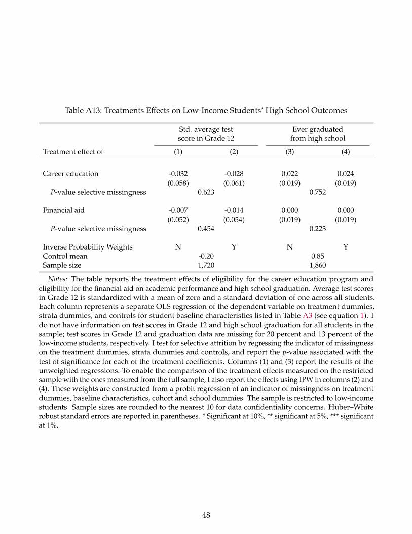
Table A13: Treatments Effects on Low-Income Students’ High School Outcomes
Std. average test Ever graduatedscore in Grade 12 from high school
Treatment effect of (1) (2) (3) (4)
Career education -0.032 -0.028 0.022 0.024(0.058) (0.061) (0.019) (0.019)
P-value selective missingness 0.623 0.752
Financial aid -0.007 -0.014 0.000 0.000(0.052) (0.054) (0.019) (0.019)
P-value selective missingness 0.454 0.223
Inverse Probability Weights N Y N YControl mean -0.20 0.85Sample size 1,720 1,860
Notes: The table reports the treatment effects of eligibility for the career education program andeligibility for the financial aid on academic performance and high school graduation. Average test scoresin Grade 12 is standardized with a mean of zero and a standard deviation of one across all students.Each column represents a separate OLS regression of the dependent variable on treatment dummies,strata dummies, and controls for student baseline characteristics listed in Table A3 (see equation 1). Ido not have information on test scores in Grade 12 and high school graduation for all students in thesample; test scores in Grade 12 and graduation data are missing for 20 percent and 13 percent of thelow-income students, respectively. I test for selective attrition by regressing the indicator of missingnesson the treatment dummies, strata dummies and controls, and report the p-value associated with thetest of significance for each of the treatment coefficients. Columns (1) and (3) report the results of theunweighted regressions. To enable the comparison of the treatment effects measured on the restrictedsample with the ones measured from the full sample, I also report the effects using IPW in columns (2) and(4). These weights are constructed from a probit regression of an indicator of missingness on treatmentdummies, baseline characteristics, cohort and school dummies. The sample is restricted to low-incomestudents. Sample sizes are rounded to the nearest 10 for data confidentiality concerns. Huber–Whiterobust standard errors are reported in parentheses. * Significant at 10%, ** significant at 5%, *** significantat 1%.
48
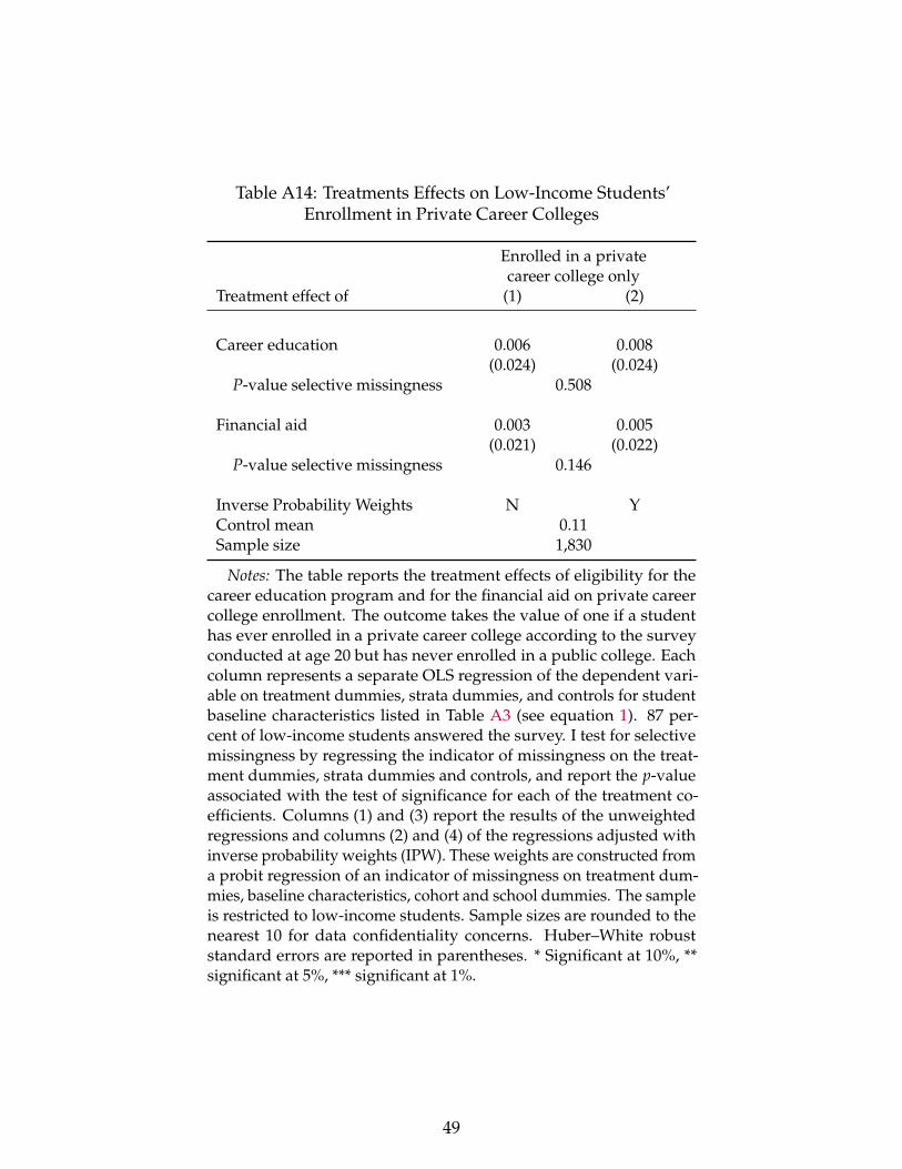
Table A14: Treatments Effects on Low-Income Students’Enrollment in Private Career Colleges
Enrolled in a privatecareer college only
Treatment effect of (1) (2)
Career education 0.006 0.008(0.024) (0.024)
P-value selective missingness 0.508
Financial aid 0.003 0.005(0.021) (0.022)
P-value selective missingness 0.146
Inverse Probability Weights N YControl mean 0.11Sample size 1,830
Notes: The table reports the treatment effects of eligibility for thecareer education program and for the financial aid on private careercollege enrollment. The outcome takes the value of one if a studenthas ever enrolled in a private career college according to the surveyconducted at age 20 but has never enrolled in a public college. Eachcolumn represents a separate OLS regression of the dependent vari-able on treatment dummies, strata dummies, and controls for studentbaseline characteristics listed in Table A3 (see equation 1). 87 per-cent of low-income students answered the survey. I test for selectivemissingness by regressing the indicator of missingness on the treat-ment dummies, strata dummies and controls, and report the p-valueassociated with the test of significance for each of the treatment co-efficients. Columns (1) and (3) report the results of the unweightedregressions and columns (2) and (4) of the regressions adjusted withinverse probability weights (IPW). These weights are constructed froma probit regression of an indicator of missingness on treatment dum-mies, baseline characteristics, cohort and school dummies. The sampleis restricted to low-income students. Sample sizes are rounded to thenearest 10 for data confidentiality concerns. Huber–White robuststandard errors are reported in parentheses. * Significant at 10%, **significant at 5%, *** significant at 1%.
49
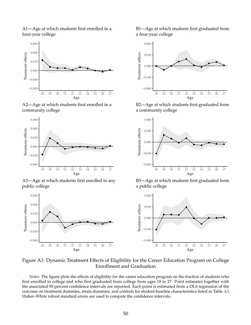
A1—Age at which students first enrolled in afour-year college
−0.060
−0.030
0.000
0.030
0.060
0.090
18 19 20 21 22 23 24 25 26 27Age
Trea
tmen
t eff
ects
B1—Age at which students first graduated froma four-year college
−0.060
−0.030
0.000
0.030
0.060
18 19 20 21 22 23 24 25 26 27Age
Trea
tmen
t eff
ects
A2—Age at which students first enrolled in acommunity college
−0.060
−0.030
0.000
0.030
0.060
0.090
18 19 20 21 22 23 24 25 26 27Age
Trea
tmen
t eff
ects
B2—Age at which students first graduated froma community college
−0.060
−0.030
0.000
0.030
0.060
18 19 20 21 22 23 24 25 26 27Age
Trea
tmen
t eff
ects
A3—Age at which students first enrolled in anypublic college
−0.060
−0.030
0.000
0.030
0.060
0.090
18 19 20 21 22 23 24 25 26 27Age
Trea
tmen
t eff
ects
B3—Age at which students first graduated froma public college
−0.060
−0.030
0.000
0.030
0.060
18 19 20 21 22 23 24 25 26 27Age
Trea
tmen
t eff
ects
Figure A1: Dynamic Treatment Effects of Eligibility for the Career Education Program on CollegeEnrollment and Graduation
Notes: The figure plots the effects of eligibility for the career education program on the fraction of students whofirst enrolled in college and who first graduated from college from ages 18 to 27. Point estimates together withthe associated 90 percent confidence intervals are reported. Each point is estimated from a OLS regression of theoutcome on treatment dummies, strata dummies, and controls for student baseline characteristics listed in Table A3.Huber–White robust standard errors are used to compute the confidence intervals.
50
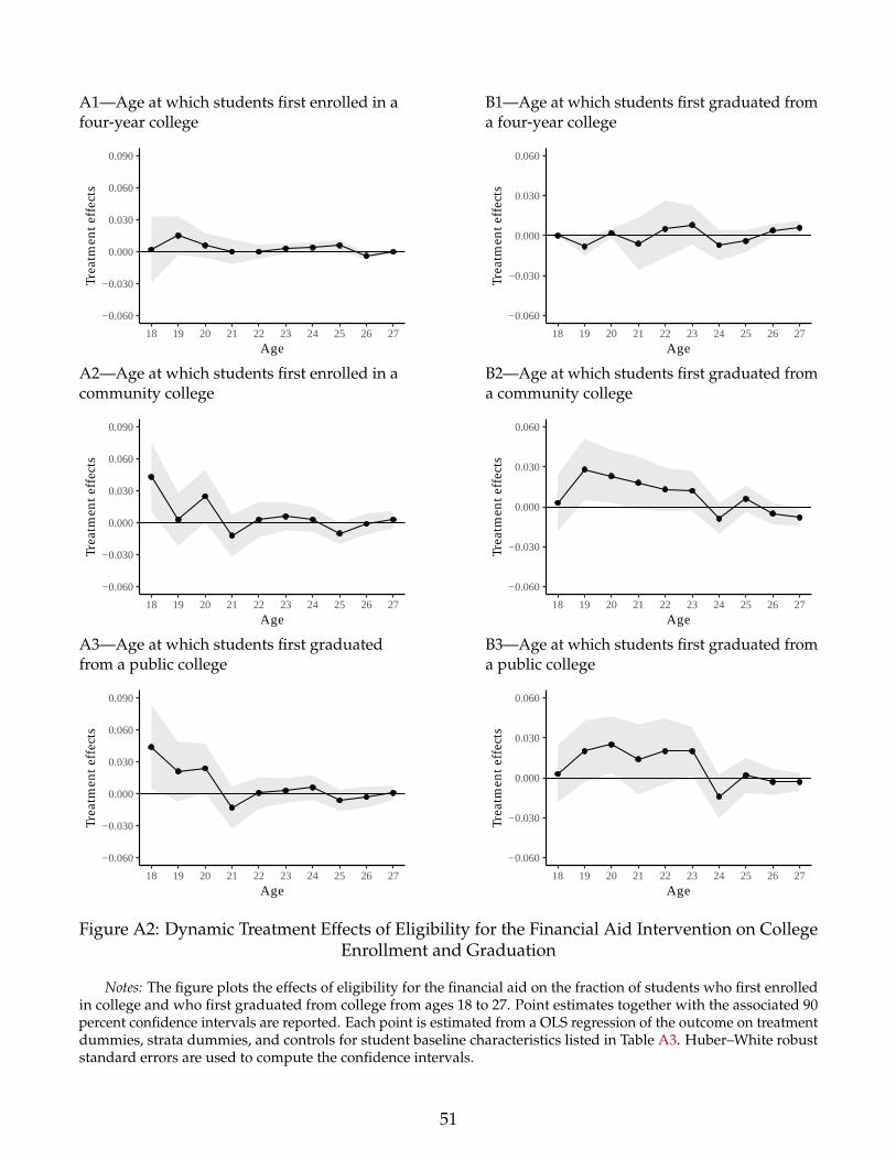
A1—Age at which students first enrolled in afour-year college
−0.060
−0.030
0.000
0.030
0.060
0.090
18 19 20 21 22 23 24 25 26 27Age
Trea
tmen
t eff
ects
B1—Age at which students first graduated froma four-year college
−0.060
−0.030
0.000
0.030
0.060
18 19 20 21 22 23 24 25 26 27Age
Trea
tmen
t eff
ects
A2—Age at which students first enrolled in acommunity college
−0.060
−0.030
0.000
0.030
0.060
0.090
18 19 20 21 22 23 24 25 26 27Age
Trea
tmen
t eff
ects
B2—Age at which students first graduated froma community college
−0.060
−0.030
0.000
0.030
0.060
18 19 20 21 22 23 24 25 26 27Age
Trea
tmen
t eff
ects
A3—Age at which students first graduatedfrom a public college
−0.060
−0.030
0.000
0.030
0.060
0.090
18 19 20 21 22 23 24 25 26 27Age
Trea
tmen
t eff
ects
B3—Age at which students first graduated froma public college
−0.060
−0.030
0.000
0.030
0.060
18 19 20 21 22 23 24 25 26 27Age
Trea
tmen
t eff
ects
Figure A2: Dynamic Treatment Effects of Eligibility for the Financial Aid Intervention on CollegeEnrollment and Graduation
Notes: The figure plots the effects of eligibility for the financial aid on the fraction of students who first enrolledin college and who first graduated from college from ages 18 to 27. Point estimates together with the associated 90percent confidence intervals are reported. Each point is estimated from a OLS regression of the outcome on treatmentdummies, strata dummies, and controls for student baseline characteristics listed in Table A3. Huber–White robuststandard errors are used to compute the confidence intervals.
51
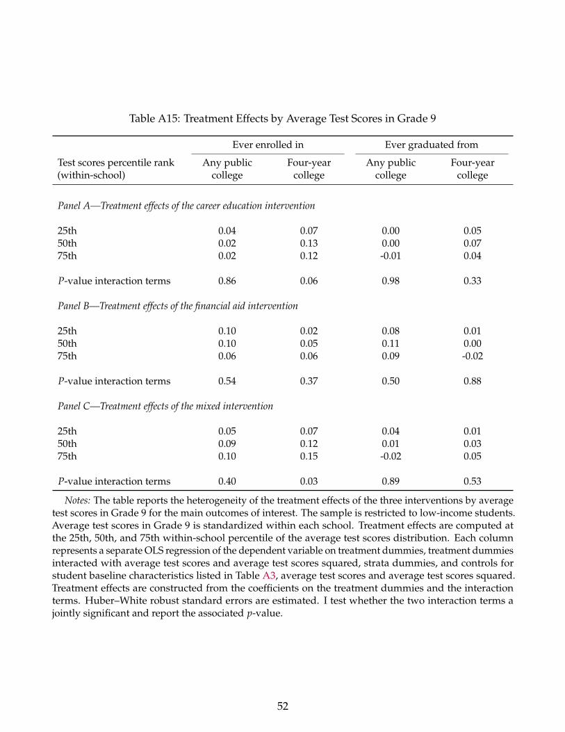
Table A15: Treatment Effects by Average Test Scores in Grade 9
Ever enrolled in Ever graduated from
Test scores percentile rank(within-school)
Any publiccollege
Four-yearcollege
Any publiccollege
Four-yearcollege
Panel A—Treatment effects of the career education intervention
25th 0.04 0.07 0.00 0.0550th 0.02 0.13 0.00 0.0775th 0.02 0.12 -0.01 0.04
P-value interaction terms 0.86 0.06 0.98 0.33
Panel B—Treatment effects of the financial aid intervention
25th 0.10 0.02 0.08 0.0150th 0.10 0.05 0.11 0.0075th 0.06 0.06 0.09 -0.02
P-value interaction terms 0.54 0.37 0.50 0.88
Panel C—Treatment effects of the mixed intervention
25th 0.05 0.07 0.04 0.0150th 0.09 0.12 0.01 0.0375th 0.10 0.15 -0.02 0.05
P-value interaction terms 0.40 0.03 0.89 0.53
Notes: The table reports the heterogeneity of the treatment effects of the three interventions by averagetest scores in Grade 9 for the main outcomes of interest. The sample is restricted to low-income students.Average test scores in Grade 9 is standardized within each school. Treatment effects are computed atthe 25th, 50th, and 75th within-school percentile of the average test scores distribution. Each columnrepresents a separate OLS regression of the dependent variable on treatment dummies, treatment dummiesinteracted with average test scores and average test scores squared, strata dummies, and controls forstudent baseline characteristics listed in Table A3, average test scores and average test scores squared.Treatment effects are constructed from the coefficients on the treatment dummies and the interactionterms. Huber–White robust standard errors are estimated. I test whether the two interaction terms ajointly significant and report the associated p-value.
52
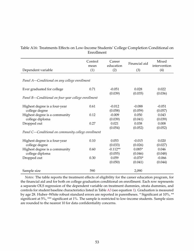
Table A16: Treatments Effects on Low-Income Students’ College Completion Conditional onEnrollment
Controlmean
Careereducation
Financial aidMixed
interventionDependent variable (1) (2) (3) (4)
Panel A—Conditional on any college enrollment
Ever graduated for college 0.71 -0.051 0.028 0.022(0.039) (0.035) (0.036)
Panel B—Conditional on four-year college enrollment
Highest degree is a four-year 0.61 -0.012 -0.088 -0.051college degree (0.058) (0.059) (0.057)
Highest degree is a community 0.12 -0.009 0.050 0.043college diploma (0.039) (0.041) (0.039)
Dropped out 0.27 0.021 0.038 0.008(0.054) (0.052) (0.052)
Panel C—Conditional on community college enrollment
Highest degree is a four-year 0.10 0.053 -0.015 0.020college degree (0.033) (0.026) (0.027)
Highest degree is a community 0.60 -0.112** 0.085* 0.046college diploma (0.055) (0.046) (0.048)
Dropped out 0.30 0.059 -0.070* -0.066(0.050) (0.041) (0.044)
Sample size 590 2,090
Notes: The table reports the treatment effects of eligibility for the career education program, forthe financial aid and for both on college graduation conditional on enrollment. Each row representsa separate OLS regression of the dependent variable on treatment dummies, strata dummies, andcontrols for student baseline characteristics listed in Table A3 (see equation 1). Graduation is measuredby age 28. Huber–White robust standard errors are reported in parentheses. * Significant at 10%, **significant at 5%, *** significant at 1%. The sample is restricted to low-income students. Sample sizesare rounded to the nearest 10 for data confidentiality concerns.
53
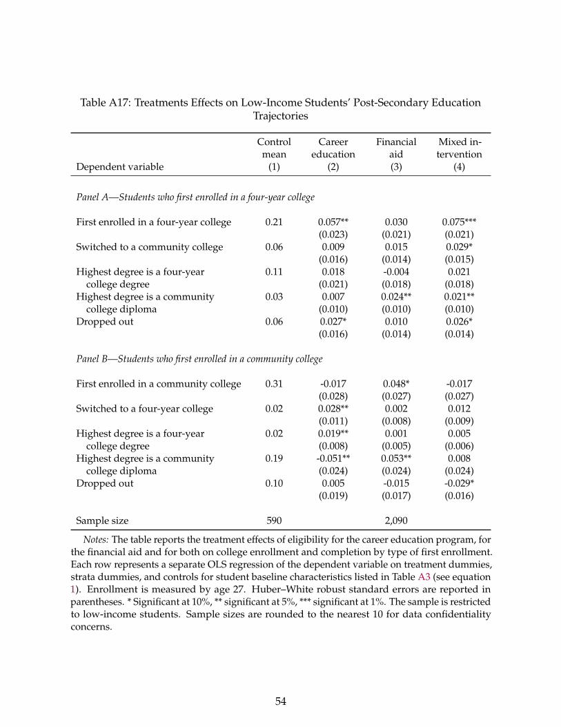
Table A17: Treatments Effects on Low-Income Students’ Post-Secondary EducationTrajectories
Controlmean
Careereducation
Financialaid
Mixed in-tervention
Dependent variable (1) (2) (3) (4)
Panel A—Students who first enrolled in a four-year college
First enrolled in a four-year college 0.21 0.057** 0.030 0.075***(0.023) (0.021) (0.021)
Switched to a community college 0.06 0.009 0.015 0.029*(0.016) (0.014) (0.015)
Highest degree is a four-year 0.11 0.018 -0.004 0.021college degree (0.021) (0.018) (0.018)
Highest degree is a community 0.03 0.007 0.024** 0.021**college diploma (0.010) (0.010) (0.010)
Dropped out 0.06 0.027* 0.010 0.026*(0.016) (0.014) (0.014)
Panel B—Students who first enrolled in a community college
First enrolled in a community college 0.31 -0.017 0.048* -0.017(0.028) (0.027) (0.027)
Switched to a four-year college 0.02 0.028** 0.002 0.012(0.011) (0.008) (0.009)
Highest degree is a four-year 0.02 0.019** 0.001 0.005college degree (0.008) (0.005) (0.006)
Highest degree is a community 0.19 -0.051** 0.053** 0.008college diploma (0.024) (0.024) (0.024)
Dropped out 0.10 0.005 -0.015 -0.029*(0.019) (0.017) (0.016)
Sample size 590 2,090
Notes: The table reports the treatment effects of eligibility for the career education program, forthe financial aid and for both on college enrollment and completion by type of first enrollment.Each row represents a separate OLS regression of the dependent variable on treatment dummies,strata dummies, and controls for student baseline characteristics listed in Table A3 (see equation1). Enrollment is measured by age 27. Huber–White robust standard errors are reported inparentheses. * Significant at 10%, ** significant at 5%, *** significant at 1%. The sample is restrictedto low-income students. Sample sizes are rounded to the nearest 10 for data confidentialityconcerns.
54
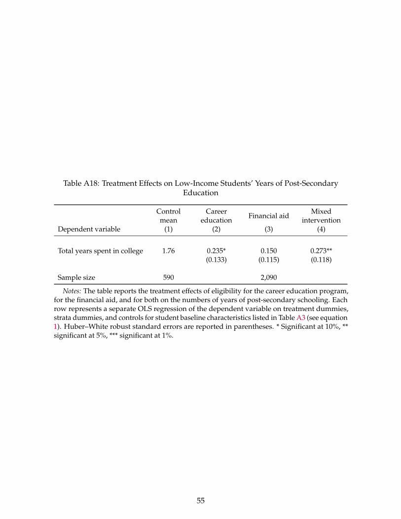
Table A18: Treatment Effects on Low-Income Students’ Years of Post-SecondaryEducation
Controlmean
Careereducation
Financial aidMixed
interventionDependent variable (1) (2) (3) (4)
Total years spent in college 1.76 0.235* 0.150 0.273**(0.133) (0.115) (0.118)
Sample size 590 2,090
Notes: The table reports the treatment effects of eligibility for the career education program,for the financial aid, and for both on the numbers of years of post-secondary schooling. Eachrow represents a separate OLS regression of the dependent variable on treatment dummies,strata dummies, and controls for student baseline characteristics listed in Table A3 (see equation1). Huber–White robust standard errors are reported in parentheses. * Significant at 10%, **significant at 5%, *** significant at 1%.
55
Table A19: Treatments Effects on Low-Income Students’ Earnings
Controlmean
Careereducation
Financial aidMixed
interventionDependent variable (1) (2) (3) (4)
Panel A— Labor income ($CA)
Labor income at age 19 10,700 -443 -357 -1,119**(556) (519) (514)
{0.880} {0.231}{0.148}
Labor income at age 24 25,500 1,551 20 147(1,691) (1,462) (1,445)
{0.371} {0.404}{0.930}
Labor income at age 28 31,700 3,265* -473 1,588(1,688) (1,477) (1,506)
{0.035} {0.346}{0.192}
Panel B—Total earnings ($CA)
Total earnings at age 19 13,300 -523 -567 -1,070*(603) (558) (558)
{0.942} {0.369}{0.372}
Total earnings at age 24 31,300 1,980 62 190(1,629) (1,412) (1,384)
{0.250} {0.274}{0.927}
Total earnings at age 28 38,200 3,631** 530 1,415(1,801) (1,483) (1,471)
{0.110} {0.251}{0.584}
Sample size 590 2,090
Notes: The table reports the treatment effects of eligibility for the career education program,for the financial aid and for both on labor income and total earnings by age. Each row representsa separate OLS regression of the dependent variable on treatment dummies, strata dummies,and controls for student baseline characteristics listed in Table A3 (see equation 1). Earningsare expressed in 2020 Canadian dollars. Huber–White robust standard errors are reported inparentheses. * Significant at 10%, ** significant at 5%, *** significant at 1%. For each outcome, Itest whether the treatment effect of each of the two financial aid interventions is significantlydifferent from the effect of the career education only intervention and report the associatedp-value below the standard errors in square brackets. I also test whether the treatment effect ofthe mixed intervention is significantly different from the effect of the financial aid interventionand report the associated p-value below the standard errors in braces. The sample is restrictedto low-income students. Sample sizes are rounded to the nearest 10 for data confidentialityconcerns.
56
Table A20: Treatment Effects on Students’ Probability ofWorking at Age 28
Low-income High-incomestudents students
Treatment group (1) (2)
Panel A—Dep. var.: Labor Income > 0
Control Mean 0.95 0.94
Treatment Effects
Career education intervention 0.001 0.000(0.014) (0.013)
Financial aid intervention -0.005(0.014)
Mixed intervention 0.002(0.013)
Panel B—Dep. var.: Labor Income > $16,000
Control Mean 0.72 0.79
Treatment Effects
Career education intervention -0.013 0.028(0.027) (0.021)
Financial aid intervention -0.038(0.026)
Mixed intervention -0.015(0.026)
Notes: The table reports the treatment effects of eligibility for thecareer education program, for the financial aid, and for both on the like-lihood of reporting any labor income and annual labor income greaterthan $16,000 which roughly corresponds to a full time job at the mini-mum wage. Each column represents a separate OLS regression of thedependent variable on treatment dummies, strata dummies, and con-trols for student baseline characteristics (see equation 1). Huber–Whiterobust standard errors are reported in parentheses. * Significant at 10%,** significant at 5%, *** significant at 1%.
57
Table A21: Robustness of the Effects on Earnings to Alternative Forecasting Models.
Career education Financial aid Mixed intervention
Mainmodel
Modelwith cov.
Simplemodel
Mainmodel
Modelwith cov.
Simplemodel
Mainmodel
Modelwith cov.
Simplemodel
Dependent variable (1) (2) (3) (4) (5) (6) (7) (8) (9)
Panel A— Low-income students
Labor income 3,265* 3,176* 3,190* -474 -533 -786 1,588 1,512 900at age 28 ($CA) (1,645) (1,688) (1,506) (1,478) (1,447) (1,474) (1,507) (1,473) (1,494)Total earnings 3,631** 3,534** 3,556** 530 426 255 1,415 1,331 781at age 28 ($CA) (1,801) (1,766) (1,802) (1,483) (1,462) (1,480) (1,471) (1,445) (1,458)
Panel B— High-income students
Labor income 2,558 2,616 2,665at age 28 ($CA) (1,633) (1,616) (1,625)Total earnings 2,788* 2,827* 2,866*at age 28 ($CA) (1,680) (1,666) (1,676)
Notes: The table reports the treatment effects of eligibility for the career education program, for the financial aid and for both onlabor income and total earnings by age, using alternative models of forecasting for the earnings data. The coefficients from Panel Aare obtained by estimating equation 1 and the ones from Panel B are obtained by estimating equation 2. Earnings are expressed in2020 Canadian dollars. Huber–White robust standard errors are reported in parentheses. * Significant at 10%, ** significant at 5%, ***significant at 1%.
58
Table A22: Prediction Error
Low-income High-incomestudents students
Treatment group (1) (2)
Panel A—Prediction Error > $5,000
Control group mean 0.251 0.273
Difference with control group
Career education intervention 0.000 -0.007(0.028) (0.024)
Financial aid intervention 0.027(0.026)
Mixed intervention 0.023(0.026)
Panel B—Prediction Error < -$5,000
Control group mean 0.259 0.332
Difference with control group
Career education intervention 0.030 0.011(0.028) (0.025)
Financial aid intervention -0.008(0.026)
Mixed intervention 0.002(0.026)
Notes: The table reports the fraction of prediction errors greaterthan $5,000 and less than -$5,000 in the control group together withthe differences in these fractions between the control group and eachtreatment group. The prediction errors are computed by taking thedifference between the value at age 24 predicted by the forecastingmodel and the true observed value, for each student. Each columnrepresents a separate OLS regression of the dependent variable ontreatment dummies. Huber–White robust standard errors are reportedin parentheses. * Significant at 10%, ** significant at 5%, *** significantat 1%.
59
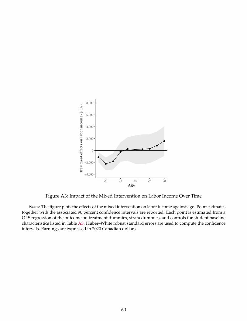
−4,000
−2,000
0
2,000
4,000
6,000
8,000
20 22 24 26 28Age
Trea
tmen
t eff
ects
on
labo
r in
com
e ($
CA
)
Figure A3: Impact of the Mixed Intervention on Labor Income Over Time
Notes: The figure plots the effects of the mixed intervention on labor income against age. Point estimatestogether with the associated 90 percent confidence intervals are reported. Each point is estimated from aOLS regression of the outcome on treatment dummies, strata dummies, and controls for student baselinecharacteristics listed in Table A3. Huber–White robust standard errors are used to compute the confidenceintervals. Earnings are expressed in 2020 Canadian dollars.
60
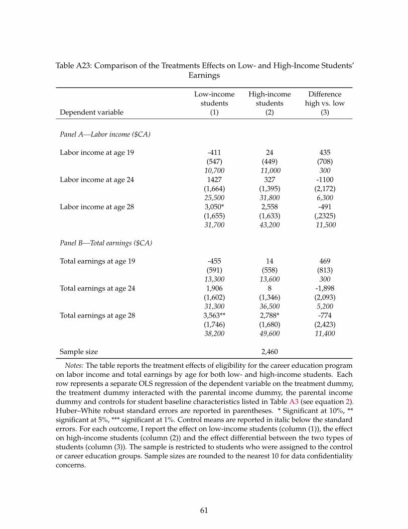
Table A23: Comparison of the Treatments Effects on Low- and High-Income Students’Earnings
Low-incomestudents
High-incomestudents
Differencehigh vs. low
Dependent variable (1) (2) (3)
Panel A—Labor income ($CA)
Labor income at age 19 -411 24 435(547) (449) (708)
10,700 11,000 300Labor income at age 24 1427 327 -1100
(1,664) (1,395) (2,172)25,500 31,800 6,300
Labor income at age 28 3,050* 2,558 -491(1,655) (1,633) (,2325)31,700 43,200 11,500
Panel B—Total earnings ($CA)
Total earnings at age 19 -455 14 469(591) (558) (813)
13,300 13,600 300Total earnings at age 24 1,906 8 -1,898
(1,602) (1,346) (2,093)31,300 36,500 5,200
Total earnings at age 28 3,563** 2,788* -774(1,746) (1,680) (2,423)38,200 49,600 11,400
Sample size 2,460
Notes: The table reports the treatment effects of eligibility for the career education programon labor income and total earnings by age for both low- and high-income students. Eachrow represents a separate OLS regression of the dependent variable on the treatment dummy,the treatment dummy interacted with the parental income dummy, the parental incomedummy and controls for student baseline characteristics listed in Table A3 (see equation 2).Huber–White robust standard errors are reported in parentheses. * Significant at 10%, **significant at 5%, *** significant at 1%. Control means are reported in italic below the standarderrors. For each outcome, I report the effect on low-income students (column (1)), the effecton high-income students (column (2)) and the effect differential between the two types ofstudents (column (3)). The sample is restricted to students who were assigned to the controlor career education groups. Sample sizes are rounded to the nearest 10 for data confidentialityconcerns.
61
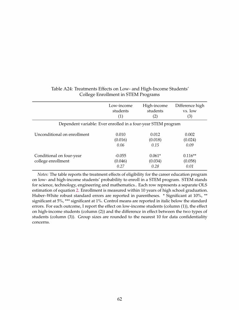
Table A24: Treatments Effects on Low- and High-Income Students’College Enrollment in STEM Programs
Low-incomestudents
High-incomestudents
Difference highvs. low
(1) (2) (3)
Dependent variable: Ever enrolled in a four-year STEM program
Unconditional on enrollment 0.010 0.012 0.002(0.016) (0.018) (0.024)
0.06 0.15 0.09
Conditional on four-year -0.055 0.061* 0.116**college enrollment (0.046) (0.034) (0.058)
0.27 0.28 0.01
Notes: The table reports the treatment effects of eligibility for the career education programon low- and high-income students’ probability to enroll in a STEM program. STEM standsfor science, technology, engineering and mathematics.. Each row represents a separate OLSestimation of equation 2. Enrollment is measured within 10 years of high school graduation.Huber–White robust standard errors are reported in parentheses. * Significant at 10%, **significant at 5%, *** significant at 1%. Control means are reported in italic below the standarderrors. For each outcome, I report the effect on low-income students (column (1)), the effecton high-income students (column (2)) and the difference in effect between the two types ofstudents (column (3)). Group sizes are rounded to the nearest 10 for data confidentialityconcerns.
62

Panel A—Career education intervention
Any college enrollment gap
0.0
0.2
0.4
0.6
0.8
1.0
0 20 40 60 80 100Within−school percentile rank
Avg
. enr
ollm
ent r
ate
Panel B—Financial aid intervention
Any college enrollment gap
0.0
0.2
0.4
0.6
0.8
1.0
0 20 40 60 80 100Within−school percentile rank
Avg
. enr
ollm
ent r
ate
Any college graduation gap
0.0
0.2
0.4
0.6
0.8
1.0
0 20 40 60 80 100Within−school percentile rank
Avg
. gra
dua
tion
rat
e
Legend
Control x LI
Control x HI
Career educ. x LI
Career educ. x HI
Any college graduation gap
0.0
0.2
0.4
0.6
0.8
1.0
0 20 40 60 80 100Within−school percentile rank
Avg
. gra
dua
tion
rat
e
Legend
Control x LI
Control x HI
Financial aid x LI
Figure A4: Enrollment Rates of High- and Low-Income Studentsby Percentile Rank and Treatment Arms
Notes: The figure plots, across within-school test scores percentile rank, the any college enrollmentand graduation rates of high- and low-income students. Panel A plots the rates for students in the careereducation group and Panel B the rates for students in the financial aid group. The enrollment rates in thecontrol group are also shown for comparability purposes. Each rate is a simple average of the rates acrossthe 30 schools, as estimated from equation A5.
63
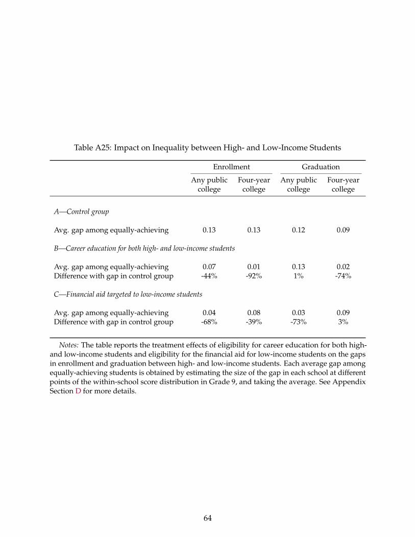
Table A25: Impact on Inequality between High- and Low-Income Students
Enrollment Graduation
Any publiccollege
Four-yearcollege
Any publiccollege
Four-yearcollege
A—Control group
Avg. gap among equally-achieving 0.13 0.13 0.12 0.09
B—Career education for both high- and low-income students
Avg. gap among equally-achieving 0.07 0.01 0.13 0.02Difference with gap in control group -44% -92% 1% -74%
C—Financial aid targeted to low-income students
Avg. gap among equally-achieving 0.04 0.08 0.03 0.09Difference with gap in control group -68% -39% -73% 3%
Notes: The table reports the treatment effects of eligibility for career education for both high-and low-income students and eligibility for the financial aid for low-income students on the gapsin enrollment and graduation between high- and low-income students. Each average gap amongequally-achieving students is obtained by estimating the size of the gap in each school at differentpoints of the within-school score distribution in Grade 9, and taking the average. See AppendixSection D for more details.
64
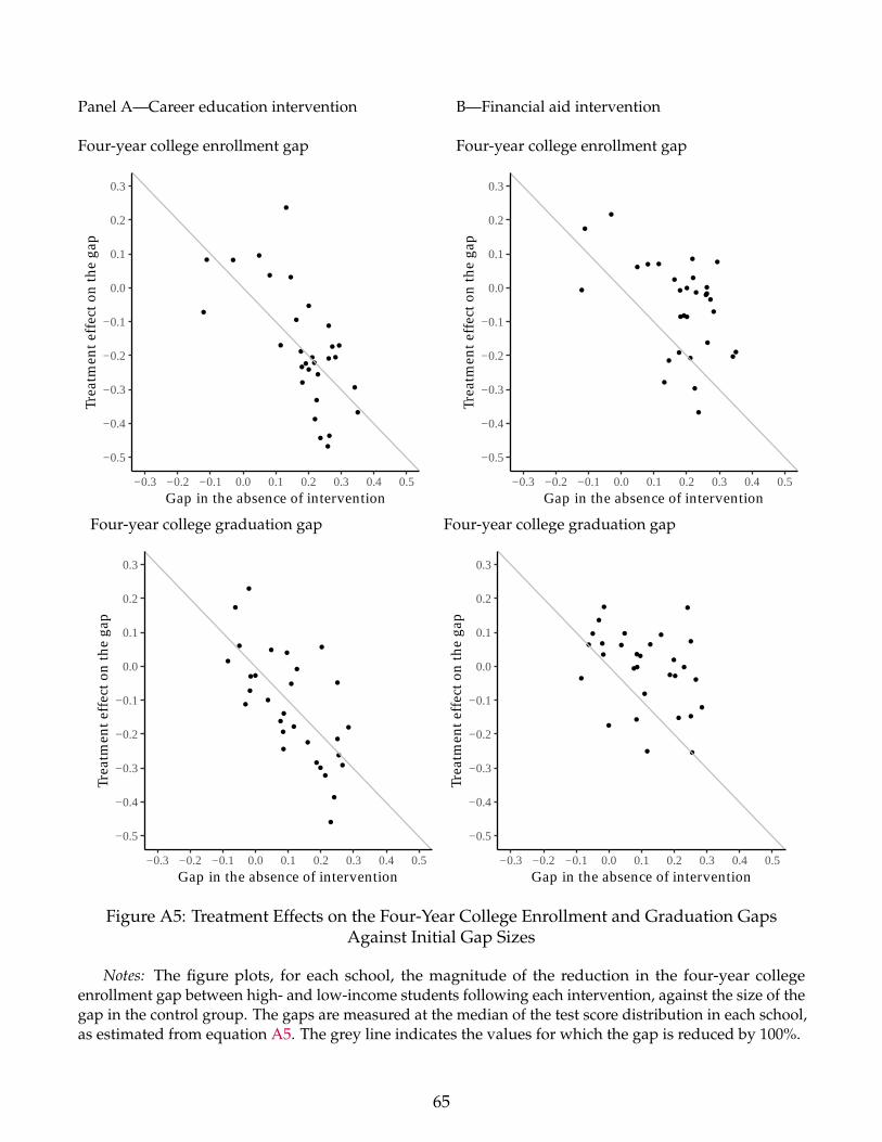
Panel A—Career education intervention
Four-year college enrollment gap
−0.5
−0.4
−0.3
−0.2
−0.1
0.0
0.1
0.2
0.3
−0.3 −0.2 −0.1 0.0 0.1 0.2 0.3 0.4 0.5Gap in the absence of intervention
Trea
tmen
t eff
ect o
n th
e ga
pB—Financial aid intervention
Four-year college enrollment gap
−0.5
−0.4
−0.3
−0.2
−0.1
0.0
0.1
0.2
0.3
−0.3 −0.2 −0.1 0.0 0.1 0.2 0.3 0.4 0.5Gap in the absence of intervention
Trea
tmen
t eff
ect o
n th
e ga
p
Four-year college graduation gap
−0.5
−0.4
−0.3
−0.2
−0.1
0.0
0.1
0.2
0.3
−0.3 −0.2 −0.1 0.0 0.1 0.2 0.3 0.4 0.5Gap in the absence of intervention
Trea
tmen
t eff
ect o
n th
e ga
p
Four-year college graduation gap
−0.5
−0.4
−0.3
−0.2
−0.1
0.0
0.1
0.2
0.3
−0.3 −0.2 −0.1 0.0 0.1 0.2 0.3 0.4 0.5Gap in the absence of intervention
Trea
tmen
t eff
ect o
n th
e ga
p
Figure A5: Treatment Effects on the Four-Year College Enrollment and Graduation GapsAgainst Initial Gap Sizes
Notes: The figure plots, for each school, the magnitude of the reduction in the four-year collegeenrollment gap between high- and low-income students following each intervention, against the size of thegap in the control group. The gaps are measured at the median of the test score distribution in each school,as estimated from equation A5. The grey line indicates the values for which the gap is reduced by 100%.
65
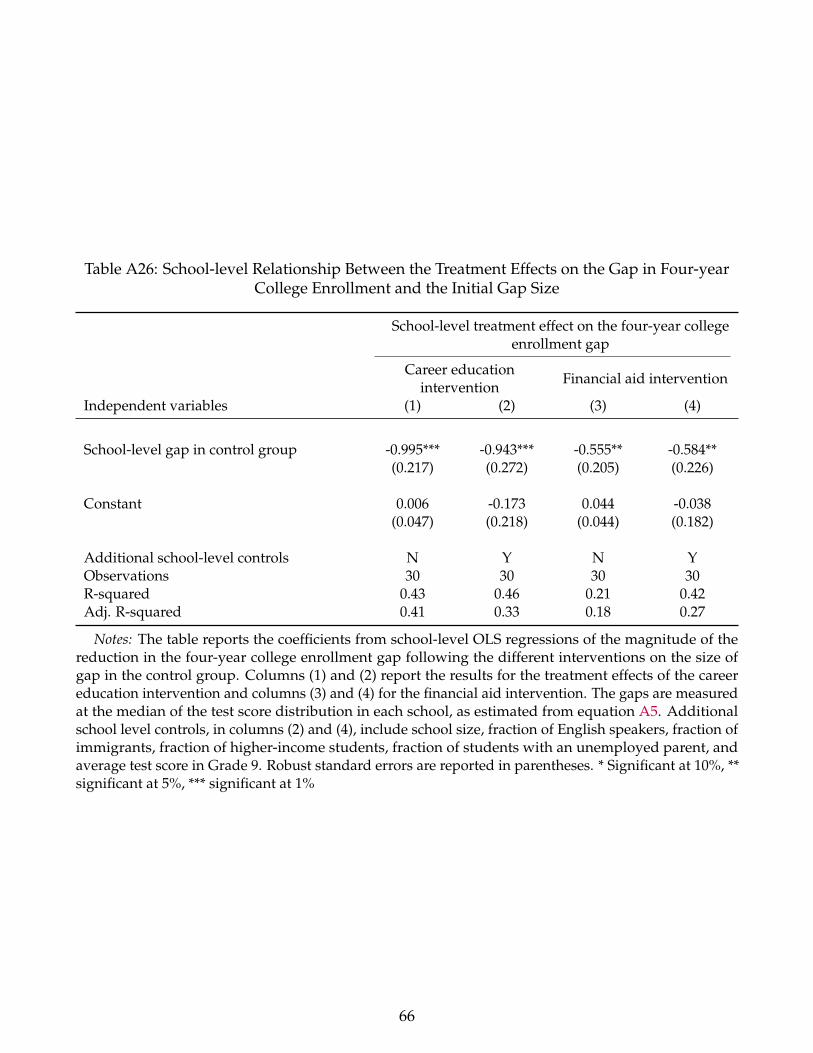
Table A26: School-level Relationship Between the Treatment Effects on the Gap in Four-yearCollege Enrollment and the Initial Gap Size
School-level treatment effect on the four-year collegeenrollment gap
Career educationintervention
Financial aid intervention
Independent variables (1) (2) (3) (4)
School-level gap in control group -0.995*** -0.943*** -0.555** -0.584**(0.217) (0.272) (0.205) (0.226)
Constant 0.006 -0.173 0.044 -0.038(0.047) (0.218) (0.044) (0.182)
Additional school-level controls N Y N YObservations 30 30 30 30R-squared 0.43 0.46 0.21 0.42Adj. R-squared 0.41 0.33 0.18 0.27
Notes: The table reports the coefficients from school-level OLS regressions of the magnitude of thereduction in the four-year college enrollment gap following the different interventions on the size ofgap in the control group. Columns (1) and (2) report the results for the treatment effects of the careereducation intervention and columns (3) and (4) for the financial aid intervention. The gaps are measuredat the median of the test score distribution in each school, as estimated from equation A5. Additionalschool level controls, in columns (2) and (4), include school size, fraction of English speakers, fraction ofimmigrants, fraction of higher-income students, fraction of students with an unemployed parent, andaverage test score in Grade 9. Robust standard errors are reported in parentheses. * Significant at 10%, **significant at 5%, *** significant at 1%
66
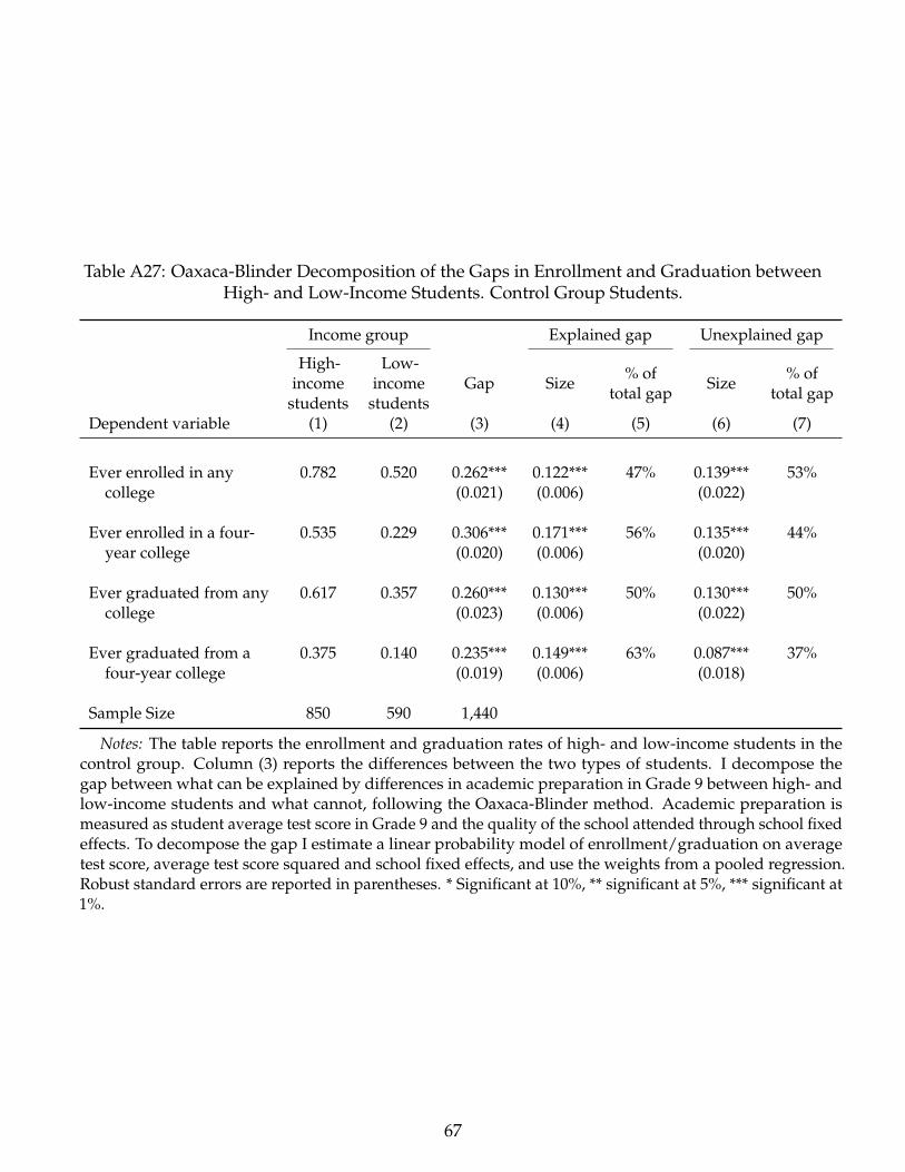
Table A27: Oaxaca-Blinder Decomposition of the Gaps in Enrollment and Graduation betweenHigh- and Low-Income Students. Control Group Students.
Income group Explained gap Unexplained gap
High-income
students
Low-income
studentsGap Size
% oftotal gap
Size% of
total gap
Dependent variable (1) (2) (3) (4) (5) (6) (7)
Ever enrolled in any 0.782 0.520 0.262*** 0.122*** 47% 0.139*** 53%college (0.021) (0.006) (0.022)
Ever enrolled in a four- 0.535 0.229 0.306*** 0.171*** 56% 0.135*** 44%year college (0.020) (0.006) (0.020)
Ever graduated from any 0.617 0.357 0.260*** 0.130*** 50% 0.130*** 50%college (0.023) (0.006) (0.022)
Ever graduated from a 0.375 0.140 0.235*** 0.149*** 63% 0.087*** 37%four-year college (0.019) (0.006) (0.018)
Sample Size 850 590 1,440
Notes: The table reports the enrollment and graduation rates of high- and low-income students in thecontrol group. Column (3) reports the differences between the two types of students. I decompose thegap between what can be explained by differences in academic preparation in Grade 9 between high- andlow-income students and what cannot, following the Oaxaca-Blinder method. Academic preparation ismeasured as student average test score in Grade 9 and the quality of the school attended through school fixedeffects. To decompose the gap I estimate a linear probability model of enrollment/graduation on averagetest score, average test score squared and school fixed effects, and use the weights from a pooled regression.Robust standard errors are reported in parentheses. * Significant at 10%, ** significant at 5%, *** significant at1%.
67
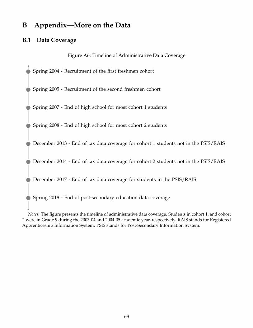
B Appendix—More on the Data
B.1 Data Coverage
Figure A6: Timeline of Administrative Data Coverage
Spring 2004 - Recruitment of the first freshmen cohort
Spring 2005 - Recruitment of the second freshmen cohort
Spring 2007 - End of high school for most cohort 1 students
Spring 2008 - End of high school for most cohort 2 students
December 2013 - End of tax data coverage for cohort 1 students not in the PSIS/RAIS
December 2014 - End of tax data coverage for cohort 2 students not in the PSIS/RAIS
December 2017 - End of tax data coverage for students in the PSIS/RAIS
Spring 2018 - End of post-secondary education data coverage
Notes: The figure presents the timeline of administrative data coverage. Students in cohort 1, and cohort2 were in Grade 9 during the 2003-04 and 2004-05 academic year, respectively. RAIS stands for RegisteredApprenticeship Information System. PSIS stands for Post-Secondary Information System.
68
B.2 Outcomes of Interest
Standardized average test scores in Grade 12: The student average test scores in Grade 12standardized with a mean of zero and a standard deviation of one across all students. Datacollected by the SRDC from the New Brunswick Department of Education.
Ever graduated from high school Indicator variable which takes the value of one if the studenthas graduated from high school at any point in time. Data collected by the SRDC from the NewBrunswick Department of Education.
Ever enrolled in any public college Indicator variable which takes the value of one if thestudent has ever enrolled in any public college within 10 years of the theoretical end of highschool (i.e., until spring 2017 for the first cohort and until spring 2018 for the second cohort).Author’s calculation from the PSIS and the data collected by the SRDC from the New BrunswickDepartment of Training and Employment Development. Exclude enrollment in private four-yearcolleges and private career colleges.
Ever enrolled in a four-year college Indicator variable which takes the value of one if thestudent has ever enrolled in a public four-year college (or university) within 10 years of thetheoretical end of high school (i.e., until spring 2017 for the first cohort and until spring 2018 forthe second cohort). Author’s calculation from the PSIS. Exclude enrollment in private four-yearcolleges.
Ever enrolled in a community college Indicator variable which takes the value of one if thestudent has ever enrolled in a community college within 10 years of the theoretical end of highschool (i.e., until spring 2017 for the first cohort and until spring 2018 for the second cohort).Author’s calculation from the PSIS and the data collected by the SRDC from the New BrunswickDepartment of Training and Employment Development.
Enrolled in a private career college only Indicator variable which takes the value of one if thestudent has ever enrolled in a private career college but never in a public college within two andhalf years of the theoretical end of high school. Author’s calculation from the survey conductedby the SRDC two and half years after the students’ theoretical end of high school.
First enrolled in a four-year college Indicator variable which takes the value of one if a stu-dent’s first enrollment in a public college is in a public four-year college (or university). Author’scalculation from the PSIS and the data collected by the SRDC from the New Brunswick Depart-ment of Training and Employment Development.
69

First enrolled in a community college Indicator variable which takes the value of one if astudent’s first enrollment in a public college is in a community college. Author’s calculation fromthe PSIS and the data collected by the SRDC from the New Brunswick Department of Trainingand Employment Development.
Enrolled in a four-year college after attending a community college Indicator variable whichtakes the value of one if a student first enrolled in a community college and later in a publicfour-year college. Author’s calculation from the PSIS and the data collected by the SRDC fromthe New Brunswick Department of Training and Employment Development.
Enrolled in a community college after attending a four-year college Indicator variable whichtakes the value of one if a student first enrolled in a public four-year college and later in acommunity college. Author’s calculation from the PSIS and the data collected by the SRDC fromthe New Brunswick Department of Training and Employment Development.
Ever graduated from a public college Indicator variable which takes the value of one if thestudent has ever graduated from a public college within 10 years of the theoretical end of highschool (i.e., until spring 2017 for the first cohort and until spring 2018 for the second cohort).Author’s calculation from the PSIS and the data collected by the SRDC from the New BrunswickDepartment of Training and Employment Development. Exclude graduation from private four-year colleges and private career colleges.
Highest degree earned is a four-year college degree Indicator variable which takes the valueof one if the student’s highest degree earned is a four-year college degree (i.e., a bachelor’s degree).Author’s calculation from the PSIS. Exclude graduation from private four-year colleges.
Highest degree earned is a community college diploma Indicator variable which takes thevalue of one if the student’s highest degree earned is a community college diploma or certificate.Author’s calculation from the PSIS and the data collected by the SRDC from the New BrunswickDepartment of Training and Employment Development. Exclude graduation from private four-year colleges and private career colleges.
Dropped out of college Indicator variable which takes the value of one if a student (i) has everenrolled in a public college, (ii) has never graduated from any public college, and (iii) is notenrolled during the 2016–17 academic year for cohort one and during the 2017–18 academic yearfor cohort two. Author’s calculation from the PSIS and the data collected by the SRDC from theNew Brunswick Department of Training and Employment Development. Exclude graduationfrom private four-year colleges and private career colleges.
70
Years spent in college It indicates the number of years a student was enrolled in a public collegewithin 10 years of the theoretical end of high school. Author’s calculation from the PSIS and thedata collected by the SRDC from the New Brunswick Department of Training and EmploymentDevelopment. Exclude years enrolled in a private institution.
Labor income It indicated the student employment income from T4 Slips. It includes all paid-employment income, i.e. wages, salaries, and commissions, before deductions and excludesself-employment income. Expressed in 2020 Canadian dollars. Data collected from the StatisticsCanada taxfiler database.
Total earnings It indicated the student total income before tax from T1 tax form. It includesemployment income, self-employment income, investment income, and government transfers(pension, unemployment insurance, child benefits, etc). Expressed in 2020 Canadian dollars. Datacollected from the Statistics Canada taxfiler database.
71
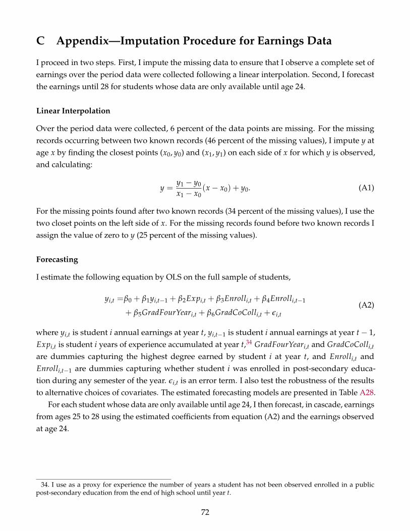
C Appendix—Imputation Procedure for Earnings Data
I proceed in two steps. First, I impute the missing data to ensure that I observe a complete set ofearnings over the period data were collected following a linear interpolation. Second, I forecastthe earnings until 28 for students whose data are only available until age 24.
Linear Interpolation
Over the period data were collected, 6 percent of the data points are missing. For the missingrecords occurring between two known records (46 percent of the missing values), I impute y atage x by finding the closest points (x0, y0) and (x1, y1) on each side of x for which y is observed,and calculating:
y =y1 − y0
x1 − x0(x− x0) + y0. (A1)
For the missing points found after two known records (34 percent of the missing values), I use thetwo closet points on the left side of x. For the missing records found before two known records Iassign the value of zero to y (25 percent of the missing values).
Forecasting
I estimate the following equation by OLS on the full sample of students,
yi,t =β0 + β1yi,t−1 + β2Expi,t + β3Enrolli,t + β4Enrolli,t−1
+ β5GradFourYeari,t + β6GradCoColli,t + εi,t(A2)
where yi,t is student i annual earnings at year t, yi,t−1 is student i annual earnings at year t− 1,Expi,t is student i years of experience accumulated at year t,34 GradFourYeari,t and GradCoColli,tare dummies capturing the highest degree earned by student i at year t, and Enrolli,t andEnrolli,t−1 are dummies capturing whether student i was enrolled in post-secondary educa-tion during any semester of the year. εi,t is an error term. I also test the robustness of the resultsto alternative choices of covariates. The estimated forecasting models are presented in Table A28.
For each student whose data are only available until age 24, I then forecast, in cascade, earningsfrom ages 25 to 28 using the estimated coefficients from equation (A2) and the earnings observedat age 24.
34. I use as a proxy for experience the number of years a student has not been observed enrolled in a publicpost-secondary education from the end of high school until year t.
72
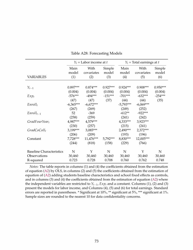
Table A28: Forecasting Models
Yt = Labor income at t Yt = Total earnings at t
Main With Simple Main With Simplemodel covariates model model covariates model
VARIABLES (1) (2) (3) (4) (5) (6)
Yt−1 0.897*** 0.874*** 0.927*** 0.924*** 0.908*** 0.950***(0.004) (0.004) (0.004) (0.004) (0.004) (0.004)
Expt -576*** -494*** -151*** -701*** -632*** -254***(47) (47) (37) (44) (44) (35)
Enrollt -6,365*** -6,672*** -5,793*** -6,069***(267) (269) (249) (252)
Enrollt−1 52 -369 -612** -922***(258) (259) (241) (242)
GradFourYeart 4,987*** 4,579*** 4,333*** 3,923***(230) (257) (215) (241)
GradCoCollt 3,199*** 3,085*** 2,490*** 2,372***(206) (209) (193) (196)
Constant 7,728*** 11,476*** 5,792*** 8,830*** 12,005***(244) (818) (158) (229) (766)
Baseline Characteristics N Y N N Y NObservations 30,460 30,460 30,460 30,460 30,460 30,460R-squared 0.723 0.728 0.708 0.760 0.762 0.748
Notes: The table reports in columns (1) and (4) the coefficients obtained from the estimationof equation (A2) by OLS, in columns (2) and (5) the coefficients obtained from the estimation ofequation of (A2) adding students baseline characteristics and school fixed effects as controls,and in columns (3) and (4) the coefficients obtained from the estimation of equation (A2) wherethe independent variables are restricted to Yt−1, Expt and a constant. Columns (1), (2) and (3)present the models for labor income, and Columns (4), (5) and (6) for total earnings. Standarderrors are reported in parentheses. * Significant at 10%, ** significant at 5%, *** significant at 1%.Sample sizes are rounded to the nearest 10 for data confidentiality concerns.
73
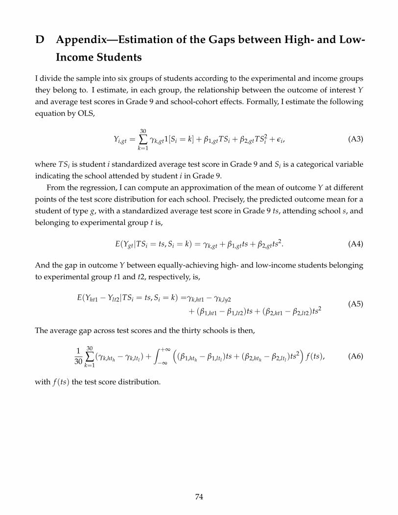
D Appendix—Estimation of the Gaps between High- and Low-
Income Students
I divide the sample into six groups of students according to the experimental and income groupsthey belong to. I estimate, in each group, the relationship between the outcome of interest Yand average test scores in Grade 9 and school-cohort effects. Formally, I estimate the followingequation by OLS,
Yi,gt =30
∑k=1
γk,gt1[Si = k] + β1,gtTSi + β2,gtTS2i + εi, (A3)
where TSi is student i standardized average test score in Grade 9 and Si is a categorical variableindicating the school attended by student i in Grade 9.
From the regression, I can compute an approximation of the mean of outcome Y at differentpoints of the test score distribution for each school. Precisely, the predicted outcome mean for astudent of type g, with a standardized average test score in Grade 9 ts, attending school s, andbelonging to experimental group t is,
E(Ygt|TSi = ts, Si = k) = γk,gt + β1,gtts + β2,gtts2. (A4)
And the gap in outcome Y between equally-achieving high- and low-income students belongingto experimental group t1 and t2, respectively, is,
E(Yht1 −Ylt2|TSi = ts, Si = k) =γk,ht1 − γk,ly2
+ (β1,ht1 − β1,lt2)ts + (β2,ht1 − β2,lt2)ts2(A5)
The average gap across test scores and the thirty schools is then,
130
30
∑k=1
(γk,hth− γk,ltl
) +∫ +∞
−∞
((β1,hth
− β1,ltl)ts + (β2,hth
− β2,ltl)ts2
)f (ts), (A6)
with f (ts) the test score distribution.
74