Embed Size (px)
Citation preview
1
The long term effect of own and spousal
parental leave on mothers’ earnings.
Andreas Kotsadama,b , Elisabeth Ugreninov a
and Henning Finseraas a
December, 2010
Abstract
We take advantage of the introduction of a Norwegian parental leave reform in 1993 to
identify the causal effect of own and spousal parental leave on mothers’ long term earnings.
The reform raised the total leave period by seven weeks, but reserved four weeks for the
father. This reform allows us to empirically examine the importance of three prominent
mechanisms proposed to explain the correlation between motherhood and wages: Human
capital depreciation, selection, and specialization. We find that women who had their last
child immediately after the policy change have substantially higher mean yearly earnings
between 1995-2005 and long run yearly earnings (from 1997 to our last year of data in 2005)
compared to women who had their last child immediately before the reform. This conclusion
is robust to using different time windows and identification strategies. By comparing our
results to the insignificant effects of another parental leave reform in 1992 that raised the total
leave period but without mandatory leave for fathers, we conclude that our results support the
specialization hypothesis.
a Norwegian Social Research, P.O. Box 3223 Elisenberg, N-0208 Oslo, Norway. Email: [email protected] [email protected] b Department of Economics, University of Gothenburg, Sweden, Box 640, SE-405 30, Gothenburg, Sweden. Email: [email protected] Acknowledgements: The paper has benefited from comments by seminar participants at Norwegian Social Reasearch (NOVA). We would also like to thank Måns Nerman, Ann-Sofie Isaksson, and Niklas Jakobsson, for useful comments.
2
1. Introduction
Why do mothers have lower earnings than childless women? Three hypotheses have been
particularly prominent in the literature. According to the depreciation hypothesis, the
interruption of the career due to maternity leave lowers wages via less work experience or
depreciation of human capital (Albrecht et al. 1999; Mincer and Polachek 1974). The
selection hypothesis argues that the correlation between motherhood and earnings (“the child
penalty” or “the family gap”) is spurious and reflects selection into motherhood (Lundberg
and Rose 2000), and perhaps into family-friendly but low-wage sectors (Nielsen et al. 2004).
Finally, the specialization hypothesis argues that the correlation is due to mothers specializing
in domestic work which make them less productive on the labor market (Becker 1985), or that
employers behave as if this is the case.
In this study we take advantage of the introduction of a Norwegian parental leave reform
which affected parents with children born after April 1st 1993, to identify the composite causal
effect of own and spousal parental leave on mothers’ earnings, and to investigate the
arguments underlying the different mechanisms used to explain the child penalty. Parental
leave has been found to lower earnings for mothers (e.g. Albrecht et al. 1999), however, most
studies are unable to control for the inherent problems of selection into parental leave and the
endogeneity of the decision to become a parent. The reform we investigate raised the total
leave period by seven weeks, but at the same time introduced a daddy quota of four weeks,
i.e. four weeks were tied to the father, and the parents lost these weeks of leave if the father
did not use them. The remaining increase of three weeks could be used by any parent and
mostly mothers’ used this extra time, as with the other transferable weeks. Thus, the nature of
this policy reform allows us to examine the strength of the different mechanisms proposed to
explain the child penalty since we identify the net long run effect of these opposing
mechanisms. If time away from work depreciates the mothers’ human capital, as the
depreciation hypothesis argues, the reform should have a negative effect on mothers’
earnings. If instead specialization is the key mechanism, we should expect the reform to
increase mothers’ earnings because mothers’ relative specialization into child-rearing is
reduced. Our identification strategy uses the fact that the reform cutoff is sharp, that the
mothers were already pregnant at the time the reform was decided upon, and that the data has
the exact day of birth for all parents of Norwegian children born around the cutoff. In
particular, the regression discontinuity design allows us to estimate the long run effects of the
reform by comparing mothers that are otherwise similar but some give birth immediately

3
before the reform and some of them give birth immediately after the reform. Selection into
having children is thereby controlled for.
Parental leave for fathers is a popular policy which has gained widespread usage around the
OECD countries, and the European Parliament recently adopted a directive stipulating a
daddy quota for four weeks (European Union 2010). Examining whether there is a causal
effect of parental leave on earnings is important, as advocates of these reforms point to such
effects, and understanding the mechanism is important since the theoretical distinction
between human capital depreciation and specialization is often hard to disentangle in practice.
In this study we are able to identify the relative magnitudes of the different mechanisms by
analyzing the reduced form effects and by investigating another parental leave reform in
1992, that raised the total leave period but without mandatory leave for fathers, we can
investigate the importance of the human capital depreciation hypothesis.
Several studies, starting with Mincer and Polachek (1974) examine the effects of career
interruptions on women’s earnings and find that long term earnings are negatively affected by
time away from work. This finding is usually interpreted as an effect of human capital
depreciation. Ruhm (1998) explores how changes in parental leave schemes affect the gender
gap in employment outcomes in nine European countries between 1963 and 1993. He finds
that parental leave increases the employment probability of women but that extended
durations (more than nine months) lower women’s wages as compared to men’s. Albrecht et
al. (1999) use Swedish data and rely on fixed effects estimations to examine the effects of
taking parental leave on mothers’ and fathers’ future wages, finding that the effect on
mothers’ wages is lower than that on fathers’ wages. Since almost all women took parental
leave in Sweden at the time there was no signaling effect for women (i.e. taking parental leave
did not signal a low attachment to the job or a low motivation for work), while parental leave
for men may have been a strong signal, since there was no daddy quota in Sweden at the time
of their data collection and very few fathers were on parental leave (1992-1993).
The main problem with the earlier studies is that they are unable to control for the inherent
problems of selection into parental leave and the endogeneity of fertility. There may be a
serious reverse causality problem if those with lower earnings choose to take more time out
from employment. We may also worry that there are omitted variables affecting both leave
4
taking and earnings, such as gender roles or that some jobs are associated with costlier
absence (Ekberg et al. 2006).
A number of more recent studies attempt to circumvent these problems by using parental
leave reforms as natural experiments. Ekberg et al. (2006) compare parents with children born
just before and just after the introduction of the Swedish daddy quota, and find strong effects
on fathers’ leave taking, but no effects on subsequent leave taken for sick children. They
interpret the latter finding as a no learning-by-doing effect of domestic labor specialization.
This interpretation is in contrast to the results Kotsadam and Finseraas (2010) who find a long
run (13 years) effect of the first Norwegian daddy quota on the division of household labor
using a similar design. A plausible interpretation of the different findings is that while
Kotsadam and Finseraas (2010) rely on various survey items of household division of labor,
Ekberg et al’s (2006) proxy for household work, leave to take care of sick children, also
involves relationship to employers. As Ekberg et al. (2006) readily admit, taking the signaling
theory as a basis for the negative effect found on earnings in previous studies, the daddy
month made a lot of fathers take parental leave, thus the signaling effect was low. Since the
reform did not affect sick leave benefits, however, taking sick leave may involve a lot of
signaling. These studies have a high internal validity, but the results regarding the long run
effects of specialization are mixed. Furthermore, these studies do not examine the wage
effects of parental leave.
Kluve and Tamm (2009) evaluate the effects of parental leave on female employment using a
German reform in 2007 with strong incentives for fathers to take parental leave. Interestingly,
they find no “long run” (2 year) effects for mothers, however, mothers are more likely to
work 1.5 years after the reform if they were subject to the reform. No effects are found for
fathers. Unfortunately, their data only include month of birth and they do not have a
representative sample of the population, as their sample is biased with regard to age, number
of children, and income. Lalive and Zweimüller (2009) use the increase of parental leave from
one to two years in 1990 and the decrease to 18 months in 1996 in Austria to investigate the
effects on employment, wages, and fertility of mothers who had their first child around the
reform dates. They find that longer parental leave increases fertility and lowers employment
and wages in the short run, but not in the long run (10 years). Moreover, the probability of
being employed is not different for the treatment and control groups from the third year
onwards, and the level of earnings is not different from the fourth year onwards. Although

5
interesting, the study does not shed any light on the effects of spousal parental leave for
women..
Johansson (2010) explores the effects of both own and spousal parental leave on earnings
using two Swedish parental leave reforms. She first controls for time-invariant heterogeneity
using fixed effects models and finds that both own and spousal parental leave affect future
earnings of parents. Interestingly, while own leave is negative for earnings, spousal leave
raises earnings, but only for women. In fact, the effect of spousal leave is found to be larger
than the effect of own leave for women. She then uses the reforms to estimate triple difference
models, using families who had their first child borne in December or January around the
reforms, which were implemented on January 1st, or one year before. The families are
observed one year before the reform and 3 years after the reform. While the estimates are
imprecise they point in the same direction as the fixed effects estimates. The fixed effects
estimates are, however, subject to critique since fertility decisions may be correlated with time
variant unobserved heterogeneity. Johansson (2010) herself gives an example whereby
fertility responds to income shocks. The more flexible triple differences model is more robust
to such criticism, but the resulting estimates become very imprecise.
Rege and Solli (2010) use Norwegian registry data to investigate the long run effects of
parental leave on full-time employed fathers’ earnings. They restrict the sample to fathers
with their youngest children between 1 and 8 years of age during the years 1992-1995. They
take advantage of the daddy quota reform in 1993 and compare earnings in a given year
between treated and non-treated fathers (based on the yearly age of children) and find that the
reform reduces fathers’ earnings by between 1 and 2.7 percent. Since the fathers in the sample
have children of different ages they estimate a difference in differences model by comparing
with the corresponding earnings difference before the daddy quota. Since their sample include
children aged between one and eight years of age, the usual difference in differences
assumption of similar time trends of fathers absent the reform is unlikely to be very reliable,
mainly because other family policies were introduced during the period and some parents
have children in school and some do not. Furthermore, they only have yearly data on time of
birth and they treat children born in 1995 as the first fully treated cohort. Lastly, they do not
investigate the impact of the reform on mothers’ earnings.
Our paper adds to the literature in several ways: The policy change used creates a natural

6
experiment that allows us to evaluate the net long run effects of both own and spousal
parental leave on mothers’ earnings; the theoretical mechanisms behind women’s child
penalty can thereby be investigated in a credible way. In terms of identification, the present
paper is the first paper to use a formal regression discontinuity design to investigate the
effects parental leave on earnings, and the present paper also stands out since it is the first
paper to investigate the effects over a longer time period. The long-term effects may be
substantial if the daddy quota reduces mother specialization into child rearing (Rege and Solli
2010) and if it affects the future division of household tasks or spousal relative human capital
endowments (Finseraas and Kotsadam 2010; Johansson 2010).
We find that the reform had significant and substantive effects on mothers’ long run earnings.
This finding lend support to the specialization hypothesis rather than the human capital
hypothesis, an interpretation that is also strengthened by the insignificant effect on earnings of
a parental leave reform in 1992 which expanded the period of leave, but with no daddy quota.
The rest of the paper is structured as follows. The next section presents the reform and
outlines our hypotheses. The following sections present the empirical strategy and the data,
the fifth section presents the results, while section six entails a broader discussion of those
results and some extensions. The final section concludes.
2. The Norwegian parental leave scheme and the 1993 reform
Norway, like the other Scandinavian countries, has for decades operated what has been
labeled as a women-friendly welfare state (Hernes 1987), where equal opportunities in
employment and domestic work has been a central topic. In Norway paid parental leave has a
long history and three historical shifts can be identified (NOU 1996). The parental leave
system was first justified with mothers’ health related necessity to be absent from work, and
to compensate for lost income in connection with pregnancy and care for small children. A
six-week paid maternity leave was introduced as far back as in 1909 and a 12-week paid
maternity leave was introduced in 1946, but only among women with health insurance. In
1956 sickness benefit became compulsory for all employed citizens, and thus a 12-week paid
maternity became available for all working women.
The second shift starts in the end of the 1960s, when the public debate for a further increase in
the number of days turned from protection of women’s health and employment to equal rights

7
in the labor market. First in 1977 fathers gained the right to use parental leave as the parental
leave was expanded to 18 weeks where only six weeks after the birth was reserved for
mothers. During the 1980s the number of weeks was increased in several rounds.
The 1990s represent the third shift in Norwegian family-work policies as the parental leave
policy turned from equal rights to equal opportunities. During the years from 1990 to 1992,
the rights to take paid parental leave were gradually extended from 28 to 35 weeks. It was a
disappointing matter of fact that an overwhelming majority of the parental leave was taken by
mothers (NOU 1995). To increase fathers’ uptake rates, Norway was the first country in the
world to introduce a “daddy quota” on 1st April 1993, where fathers to children born at or
after this date got an independent right to parental leave. The reform extends the parental
leave from 35 to 42 weeks with full earnings compensation (up to a ceiling of 6 times the
basic amount, although many employers compensate for the remaining part), of which four
weeks were reserved for the father. 1 At this time, paid paternity leave was contingent on both
parents working at least 50 percent before the child was born, and payment to fathers were
reduced if the mother did not work full time. Fathers were entitled to use the daddy quota up
until the child turned 3 years of age although 95 percent of those taking leave in 1993-1995
did so during the child’s first year (Rege and Solli 2010).
More caring fathers were seen as an important step on the way to equal division of labor and
towards reducing the wage gap. The political arguments to earmark some of the parental leave
for fathers were threesome; firstly, this policy implementation gives a strong signal and
possibilities to be more active involved in child caring and hence challenge norms of male
breadwinning (Leira 1998; Leira 2008; Hook 2010). Secondly, an independent right to
parental leave gives fathers an advantage when parents discuss the distribution of the parental
leave between them. Thirdly, the law strengthens fathers’ argument for parental leave with
reluctant employers. The reform led to a sharp increase in the uptake rate from less than four
percent prior to the reform to 70 percent in 1995 (Brunning and Plantenga 1999).
1 In fact, parents could choose to either take the 42 weeks with full compensation or 52 weeks with 80 % earnings compensation. Note that the choice between taking a shorter period with full coverage or a longer period with less coverage has been available since 1989 and was not a new feature of this reform.

8
3. Empirical strategy
Since all parents who had their last (latest) child after the reform date were treated by the
reform and no parents who had their last child before the reform date were treated, we can
compare the two groups of parents in order to identify the causal effects of the policy. We
also exploit the fact that the policy process was fast so that parents giving birth around the
reform threshold could not have known about the reform at the time of conception. The
specific design, including 1st of April 1993 as the day of implementation, was proposed on the
1st of December 1992, and decided in parliament the 22nd of January 1993.2
We start by running OLS regressions of earnings on treatment for groups having children just
before and just after the reform. The equation to be estimated is thus:
ii TreatmentEarnings X ii
Where Treatment is an indicator variable which equals one for those having children just after
the reform in 1993, X is a vector of predetermined variables (the age of the parents at the
time of birth, number of children before 1993, and lagged values of income), and i is an error
term. The sample windows presented in the main analyses are chosen to be two weeks, six
weeks, and three months. (Results with even shorter time windows are presented in the
Appendix).
The two weeks sample is our “random” sample. It corresponds well with what Rosenzweig
and Wolpin (2000) label a “natural” natural experiment whereby nature determines which
side of the cut-off people end up at. First of all, it is not possible for parents to completely
control the date of conception (Eriksson 2005; Lalive and Zweimüller 2009). Secondly, a
pregnancy takes on average 40 weeks and the duration is normally distributed with a standard
deviation of two weeks (Ekberg et al. 2006; Eriksson 2005). Most importantly, none of the
parents knew that they would be treated at the time of conception. Thereby the reform creates
exogenous variation in own and spousal parental leave and long-run differences in outcomes
can plausibly be attributed to the change in legislation (cf. Kluve and Tamm 2009 and Lalive 2 The Government first proposed to introduce a daddy quota of four weeks in the state budget for 1993 which was accepted by the Norwegian parliament on the 4th of November 1992 (Budsjett-innst. S. nr.2 1992-1993). At this time, however, the exact date of implementation was not known.

9
and Zweimüller 2009). Births can not be postponed and the reform we study is strictly
favorable for parents so triggering of birth by medical means such as by a caesarian section
(see Johansson 2010) should not be a problem.
In the three months sample there is a statistically significant difference between the groups
with respect to the parents’ age. In the other samples this is not the case. We choose to present
results both with and without parents’ age in 1993 since it is predetermined and plausibly
exogenous. Including exogenous variables is likely to increase the precision of the estimates
without biasing the treatment coefficient.
We also use the reform in a sharp regression discontinuity (RD) design as the treatment of
being offered a daddy quota and a prolonged leave is a deterministic and discontinuous
function of the birth date. That is, we center the treatment at day zero for April 1st which
yields:
0 0
0 1
i
ii daysif
daysifTreatment
The forcing variable, days, is expected to be negatively associated with earnings as parents of
younger children are younger and since they have a higher workload at home. Importantly,
however, the relationship between days and earnings is assumed to be smooth so that any
discontinuity at the threshold can be attributed to the causal effect of the parental leave
reform. In our case, the continuous effect of days is controlled for by estimating:
iiiiii TreatmentdaysTreatmentdaysaEarnings * ,
The smoothness assumption allows us to estimate the difference between two regression
functions at day 0. is still our parameter of interest and it is identified by separating the
continuous function of days from the discontinuity imposed by the treatment. By including
the interaction term between days and Treatment we allow the slope coefficients to differ on
each side of the threshold. This is the same as estimating the two regression functions below
and calculating the difference in intercepts (a1-a2):

10
0 1 iiii daysifdaysaEarnings
0 2 iiii daysifdaysaEarnings
A first step in the RD will be to estimate the earnings equation with the linear time trend and
samples close to the cutoff. This local linear regression approach is less likely to be valid with
larger bandwidths, unless we know that the underlying function for the forcing variable is
indeed linear, and the robustness should be checked by varying the time window (Lee and
Lemieux 2010).
The function for days does not have to be linear, and we relax the linearity assumption by
including polynomial functions of days in the regression model. That is, in order to assess the
robustness of the treatment effect, we also estimate 2nd, 3rd, and 4th order polynomial
functions. Comparing the RD results to the results of a ”discontinuity sample”, with
observations close to the discontinuity such as the two weeks sample, is an important
robustness check, since the treatment effect in such a sample does not depend on neither the
model specification nor a constant effects assumption (Angrist and Pischke 2009).
One potential problem for identification of causal effects of the reform is that there is a
difference between parents to children born at different times. This difference arises by
construction in our data since one group always has younger children when the data is
collected at the end of the year. We deal with this issue by presenting regression results on
falsification samples where those included had children either around the month before or the
month after the reform. These “placebo” regressions should yield statistically insignificant
results as the groups are facing the same parental leave regulation. Finally, neither of the
approaches discussed thus far account for possible biological or social differences between
parents of children born in March or April. To account for such differences we also present
regression results on falsification samples where those included had children around the same
dates but one year after the reform.
4. Data, samples, and descriptive statistics
We rely on high quality register data encompassing all individuals in Norway. The data is
gathered from several administrative registers used to calculate taxes, pension rights, and
unemployment benefits and attrition, self-report problems and bias due to refusal to
participate in the study are non-existent.

11
Our dependent variables are derived from two different measures; yearly income based on
accumulation of pension (Personal income), and yearly labor income. Both measures are
gross of taxes and they are measured at the end of the year. Personal income mainly includes
employment income and income from self-employment. In addition, unemployment benefit,
sickness benefit, maternity benefit and adoption allowance are included and it is also possible
to acquire accumulation of pension on the basis of non paid caring work for family members.
Another disadvantage, in addition to not only measuring income stemming from work, is that
personal income is left and right censored. Incomes below or equal to one basic amount and
above or equal to 12 basic amounts does not qualify for accumulation of pension and
therefore do not enter in the measure of Personal income. Labor income includes wages and
salaries from paid employment, and net entrepreneurial income. From the Labor income
variable we create our two main dependent variables; Earnings 2005 which is simply labor
income in 2005 and Mean earnings, which is the mean yearly labor income between 1995 and
2005. The use of Personal income is restricted to estimations including observations before
1993, where it has to be used since Labor income is only available from 1993 and onwards.
The data includes information on the exact day of birth of all children born in Norway. We
restrict our sample to individuals where we have information about both parents and children
born in Norway. As mentioned in the empirical strategy we focus on samples with parents of
children born close to the reform cutoff and only on children born in the same year to
minimize other confounding factors such as different school enrolment years. Furthermore,
we focus on parents of their last born child in 1993 since those who also have children later
on are affected by the treatment as well. Only investigating the effects for those with their last
born child is necessary in order to have a clean comparison between treated and control
individuals but it may be problematic to generalize the results to the total population if the
reform affected the total fertility rate. This is so since our sample then consists of a special
type of individuals not affected in their fertility decision by the reform. It is also problematic
if the reform affects mothers differently depending on whether they have other children or
not. If the reform affects mothers of their first born child more than other mothers we are
likely to underestimate the effect of the reform and if the reform affected mothers who already
had other children more we may be overestimating the treatment effect. We investigate the
fertility rate issue by comparing all mothers who had a child around the reform and find no
difference between mothers having a child just before or just after the reform in the number of

12
children they have after the reform. This is important since it implies that those affected by
the reform are not different in their fertility pattern from those in the control group, a crucial
feature for the internal validity of the estimation strategy. With respect to issues of external
validity the question of different effects at different birth parities is investigated further in
section 6.2.
Table 1: Summary statistics of treatment and control groups for different time windows.
Control groups Treatment groups Three months sample. Variable N Mean Std. Dev. N Mean Std. Dev. Earnings 2005 5938 244315.1** 173948.1 6474 250791.4 190943.7 Mean earnings 5938 175567.5 111368.5 6474 178034.7 114297.5 Mothers’ age 93 5938 31.187*** 4.849 6474 30.856 4.802 Fathers’ age 93 5938 33.947** 5.798 6474 33.636 5.806 Nr of children before 5938 1.217 0.847 6474 1.214 0.854 Personal income 1988 5938 80458.18 64894.46 6474 81966.15 64835.14 Six weeks sample. N Mean Std. Dev. N Mean Std. Dev. Earnings 2005 3164 242198.1** 165031.9 3213 251769 205356.4 Mean earnings 3164 174304.8* 110167.4 3213 179033.8 115869.0 Mothers’ age 93 3164 31.047 4.846 3213 30.924 4.716 Fathers’ age 93 3164 33.729 5.781 3213 33.841 5.829 Nr of children before 3164 1.217 0.842 3213 1.223 0.847 Personal income 1988 3164 80456.71 64653.62 3213 81823.46 64909.02 Two weeks sample. N Mean Std. Dev. N Mean Std. Dev. Earnings 2005 1000 245333.3* 160250.4 1065 261833.1 222404.8 Mean earnings 1000 176699.1** 109950.7 1065 187752.5 129104.4 Mothers’ age 93 1000 31.011 4.865 1065 30.896 4.707 Fathers’ age 93 1000 33.666 5.774 1065 33.876 5.776 Nr of children before 1000 1.229 0.831 1065 1.234 0.814 Personal income 1988 1000 78914.3 63075.13 1065 79969.78 65660.91
*** p<0.01, ** p<0.05, * p<0.1 (p-values in two-sided t-tests of the difference between treatment and control groups).
We present summary statistics by treatment status for our three main samples in Table 1. We
see that the mothers in the treatment group have higher yearly earnings in 2005 (our last year
of data) and higher mean earnings between the years 1995-2005 than mothers in the control
group (note, however, that the second difference is not statistically significant at conventional
levels in the three months sample). We also see that there is a difference between the parents

13
in the treatment and control groups with respect to their age at the time of birth in the three
months sample. No such difference is present for the shorter time windows, however and the
samples are also balanced in the number of children they had before the last child is born.
Finally, it is reassuring to see that the mothers in the treatment and control cohorts do not
have statistically significant different personal income in 1988 (we do not have data on labor
income before 1993).
A crucial assumption of the identification strategy is that the reform is exogenous and hence
that the density function of the forcing variable, days, is continuous. If agents are able to
manipulate the time of birth, the continuity assumption underlying identification may be
violated. As already discussed, it is unlikely that parents could precisely manipulate the time
of birth since it is not possible for parents to completely control the date of conception and
since none of the parents knew that they would be treated at the time of conception.
Nonetheless, Figure 1 shows histograms of the forcing variable with different bin widths (4.5
days and 1 day) and a visual inspection of the densities for days also suggests that parents did
not manipulate the time of birth.
0.0
02.0
04.0
06.0
08D
ens
ity
-100 -50 0 50 100days
Histogram for days (binwidth 4.5 days, 40 bins)
0.0
02.0
04.0
06.0
08.0
1D
ens
ity
-100 -50 0 50 100days
Histogram for days (binwidth 1 day, 180 bins)
Figure 1: Histograms for days
14
5. Results
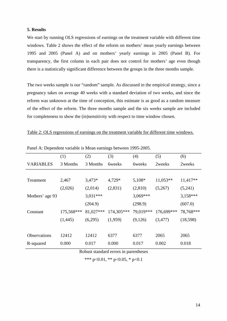
We start by running OLS regressions of earnings on the treatment variable with different time
windows. Table 2 shows the effect of the reform on mothers’ mean yearly earnings between
1995 and 2005 (Panel A) and on mothers’ yearly earnings in 2005 (Panel B). For
transparency, the first column in each pair does not control for mothers’ age even though
there is a statistically significant difference between the groups in the three months sample.
The two weeks sample is our “random” sample. As discussed in the empirical strategy, since a
pregnancy takes on average 40 weeks with a standard deviation of two weeks, and since the
reform was unknown at the time of conception, this estimate is as good as a random measure
of the effect of the reform. The three months sample and the six weeks sample are included
for completeness to show the (in)sensitivity with respect to time window chosen.
Table 2: OLS regressions of earnings on the treatment variable for different time windows.
Panel A: Dependent variable is Mean earnings between 1995-2005.
(1) (2) (3) (4) (5) (6)
VARIABLES 3 Months 3 Months 6weeks 6weeks 2weeks 2weeks
Treatment 2,467 3,473* 4,729* 5,108* 11,053** 11,417**
(2,026) (2,014) (2,831) (2,810) (5,267) (5,241)
Mothers’ age 93 3,031*** 3,069*** 3,158***
(204.9) (298.9) (607.0)
Constant 175,568*** 81,027*** 174,305*** 79,019*** 176,699*** 78,768***
(1,445) (6,295) (1,959) (9,126) (3,477) (18,598)
Observations 12412 12412 6377 6377 2065 2065
R-squared 0.000 0.017 0.000 0.017 0.002 0.018
Robust standard errors in parentheses
*** p<0.01, ** p<0.05, * p<0.1
15
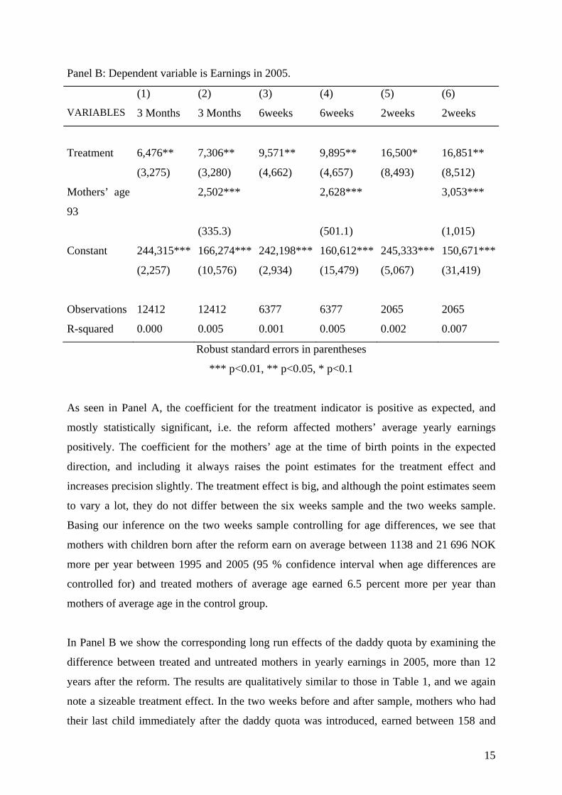
Panel B: Dependent variable is Earnings in 2005.
(1) (2) (3) (4) (5) (6)
VARIABLES 3 Months 3 Months 6weeks 6weeks 2weeks 2weeks
Treatment 6,476** 7,306** 9,571** 9,895** 16,500* 16,851**
(3,275) (3,280) (4,662) (4,657) (8,493) (8,512)
Mothers’ age
93
2,502*** 2,628*** 3,053***
(335.3) (501.1) (1,015)
Constant 244,315*** 166,274*** 242,198*** 160,612*** 245,333*** 150,671***
(2,257) (10,576) (2,934) (15,479) (5,067) (31,419)
Observations 12412 12412 6377 6377 2065 2065
R-squared 0.000 0.005 0.001 0.005 0.002 0.007
Robust standard errors in parentheses
*** p<0.01, ** p<0.05, * p<0.1
As seen in Panel A, the coefficient for the treatment indicator is positive as expected, and
mostly statistically significant, i.e. the reform affected mothers’ average yearly earnings
positively. The coefficient for the mothers’ age at the time of birth points in the expected
direction, and including it always raises the point estimates for the treatment effect and
increases precision slightly. The treatment effect is big, and although the point estimates seem
to vary a lot, they do not differ between the six weeks sample and the two weeks sample.
Basing our inference on the two weeks sample controlling for age differences, we see that
mothers with children born after the reform earn on average between 1138 and 21 696 NOK
more per year between 1995 and 2005 (95 % confidence interval when age differences are
controlled for) and treated mothers of average age earned 6.5 percent more per year than
mothers of average age in the control group.
In Panel B we show the corresponding long run effects of the daddy quota by examining the
difference between treated and untreated mothers in yearly earnings in 2005, more than 12
years after the reform. The results are qualitatively similar to those in Table 1, and we again
note a sizeable treatment effect. In the two weeks before and after sample, mothers who had
their last child immediately after the daddy quota was introduced, earned between 158 and
16
33 545 NOK (approximately 26 and 5007 dollars) in 2005 (95 % confidence interval when
age differences are controlled for) more than mothers who gave birth to their latest child
immediately before the reform and treated mothers of average age earned 6.9 percent more in
2005 than mothers of average age in the control group.
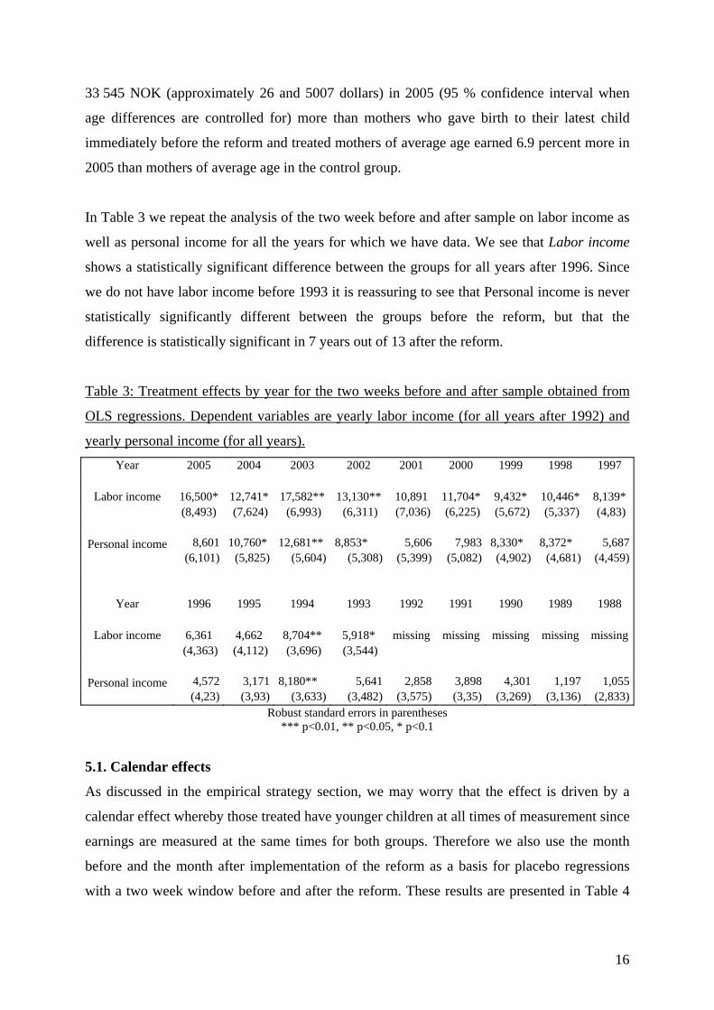
In Table 3 we repeat the analysis of the two week before and after sample on labor income as
well as personal income for all the years for which we have data. We see that Labor income
shows a statistically significant difference between the groups for all years after 1996. Since
we do not have labor income before 1993 it is reassuring to see that Personal income is never
statistically significantly different between the groups before the reform, but that the
difference is statistically significant in 7 years out of 13 after the reform.
Table 3: Treatment effects by year for the two weeks before and after sample obtained from
OLS regressions. Dependent variables are yearly labor income (for all years after 1992) and
yearly personal income (for all years).
Year 2005 2004 2003 2002 2001 2000 1999 1998 1997
Labor income 16,500* 12,741* 17,582** 13,130** 10,891 11,704* 9,432* 10,446* 8,139* (8,493) (7,624) (6,993) (6,311) (7,036) (6,225) (5,672) (5,337) (4,83)
Personal income 8,601 10,760* 12,681** 8,853* 5,606 7,983 8,330* 8,372* 5,687
(6,101) (5,825) (5,604) (5,308) (5,399) (5,082) (4,902) (4,681) (4,459)
Year 1996 1995 1994 1993 1992 1991 1990 1989 1988
Labor income 6,361 4,662 8,704** 5,918* missing missing missing missing missing (4,363) (4,112) (3,696) (3,544)
Personal income 4,572 3,171 8,180** 5,641 2,858 3,898 4,301 1,197 1,055
(4,23) (3,93) (3,633) (3,482) (3,575) (3,35) (3,269) (3,136) (2,833)Robust standard errors in parentheses
*** p<0.01, ** p<0.05, * p<0.1
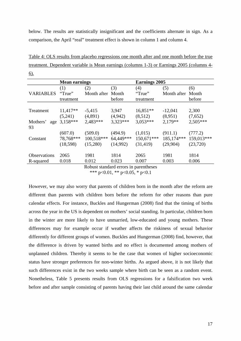
5.1. Calendar effects
As discussed in the empirical strategy section, we may worry that the effect is driven by a
calendar effect whereby those treated have younger children at all times of measurement since
earnings are measured at the same times for both groups. Therefore we also use the month
before and the month after implementation of the reform as a basis for placebo regressions
with a two week window before and after the reform. These results are presented in Table 4
17
below. The results are statistically insignificant and the coefficients alternate in sign. As a
comparison, the April “real” treatment effect is shown in column 1 and column 4.
Table 4: OLS results from placebo regressions one month after and one month before the true
treatment. Dependent variable is Mean earnings (columns 1-3) or Earnings 2005 (columns 4-
6).
Mean earnings Earnings 2005 (1) (2) (3) (4) (5) (6) VARIABLES “True”
treatment Month after Month
before “True” treatment
Month after Month before
Treatment 11,417** -5,415 3,947 16,851** -12,041 2,300 (5,241) (4,891) (4,942) (8,512) (8,951) (7,652) Mothers’ age 93
3,158*** 2,483*** 3,323*** 3,053*** 2,179** 2,505***
(607.0) (509.0) (494.9) (1,015) (911.1) (777.2) Constant 78,768*** 100,518*** 64,449*** 150,671*** 185,174*** 159,013*** (18,598) (15,280) (14,992) (31,419) (29,904) (23,720) Observations 2065 1981 1814 2065 1981 1814 R-squared 0.018 0.012 0.023 0.007 0.003 0.006
Robust standard errors in parentheses *** p<0.01, ** p<0.05, * p<0.1
However, we may also worry that parents of children born in the month after the reform are
different than parents with children born before the reform for other reasons than pure
calendar effects. For instance, Buckles and Hungerman (2008) find that the timing of births
across the year in the US is dependent on mothers’ social standing. In particular, children born
in the winter are more likely to have unmarried, low-educated and young mothers. These
differences may for example occur if weather affects the riskiness of sexual behavior
differently for different groups of women. Buckles and Hungerman (2008) find, however, that
the difference is driven by wanted births and no effect is documented among mothers of
unplanned children. Thereby it seems to be the case that women of higher socioeconomic
status have stronger preferences for non-winter births. As argued above, it is not likely that
such differences exist in the two weeks sample where birth can be seen as a random event.
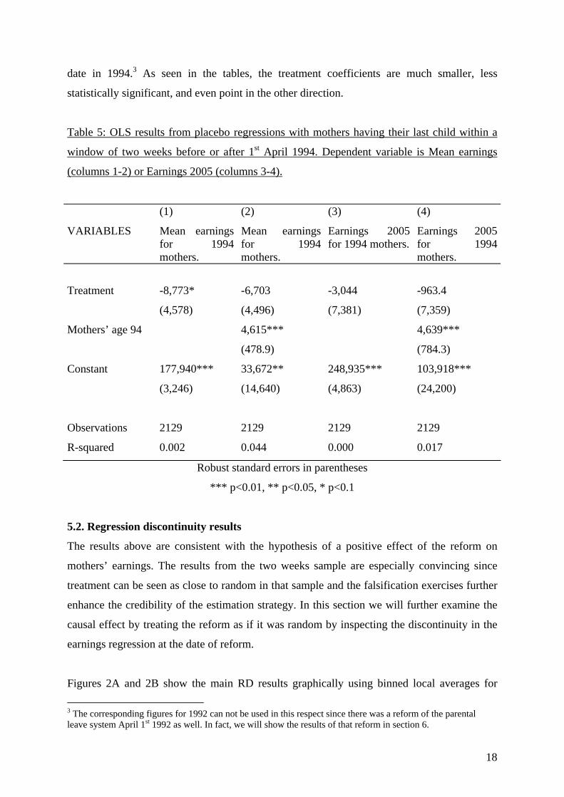
Nonetheless, Table 5 presents results from OLS regressions for a falsification two week
before and after sample consisting of parents having their last child around the same calendar
18
date in 1994.3 As seen in the tables, the treatment coefficients are much smaller, less
statistically significant, and even point in the other direction.
Table 5: OLS results from placebo regressions with mothers having their last child within a
window of two weeks before or after 1st April 1994. Dependent variable is Mean earnings
(columns 1-2) or Earnings 2005 (columns 3-4).
(1) (2) (3) (4)
VARIABLES Mean earnings for 1994 mothers.
Mean earnings for 1994 mothers.
Earnings 2005 for 1994 mothers.
Earnings 2005 for 1994 mothers.
Treatment -8,773* -6,703 -3,044 -963.4
(4,578) (4,496) (7,381) (7,359)
Mothers’ age 94 4,615*** 4,639***
(478.9) (784.3)
Constant 177,940*** 33,672** 248,935*** 103,918***
(3,246) (14,640) (4,863) (24,200)
Observations 2129 2129 2129 2129
R-squared 0.002 0.044 0.000 0.017
Robust standard errors in parentheses
*** p<0.01, ** p<0.05, * p<0.1
5.2. Regression discontinuity results
The results above are consistent with the hypothesis of a positive effect of the reform on
mothers’ earnings. The results from the two weeks sample are especially convincing since
treatment can be seen as close to random in that sample and the falsification exercises further
enhance the credibility of the estimation strategy. In this section we will further examine the
causal effect by treating the reform as if it was random by inspecting the discontinuity in the
earnings regression at the date of reform.
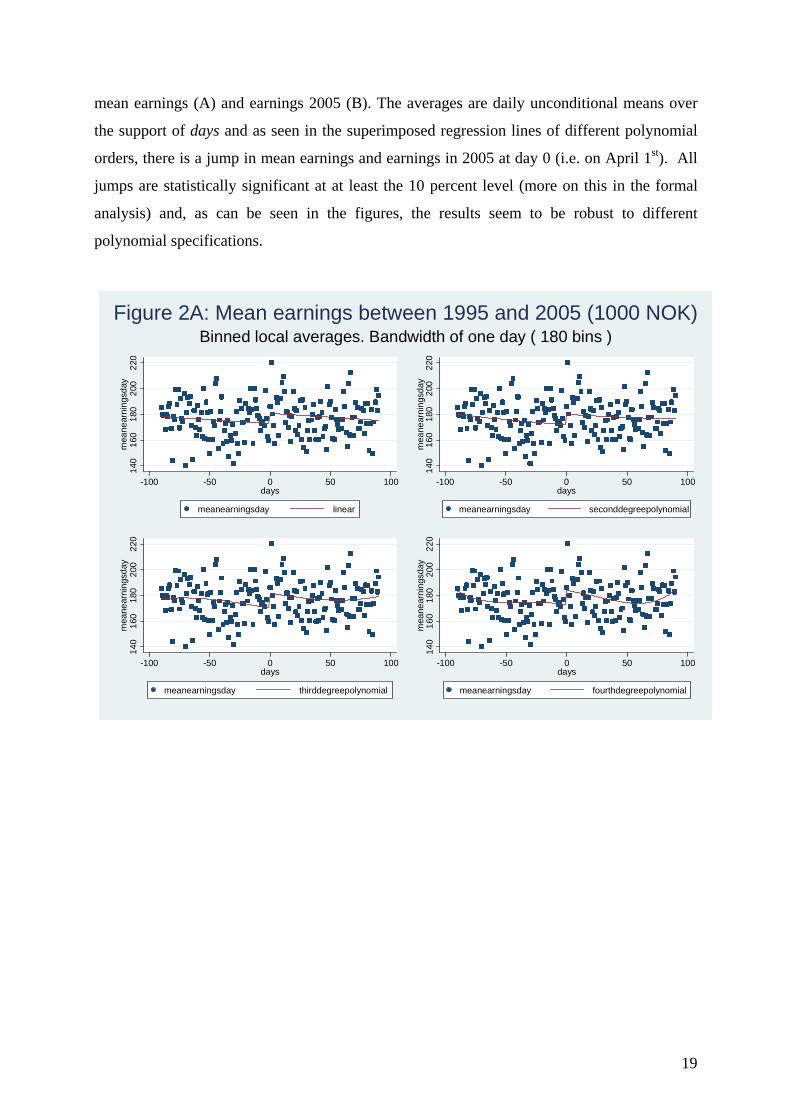
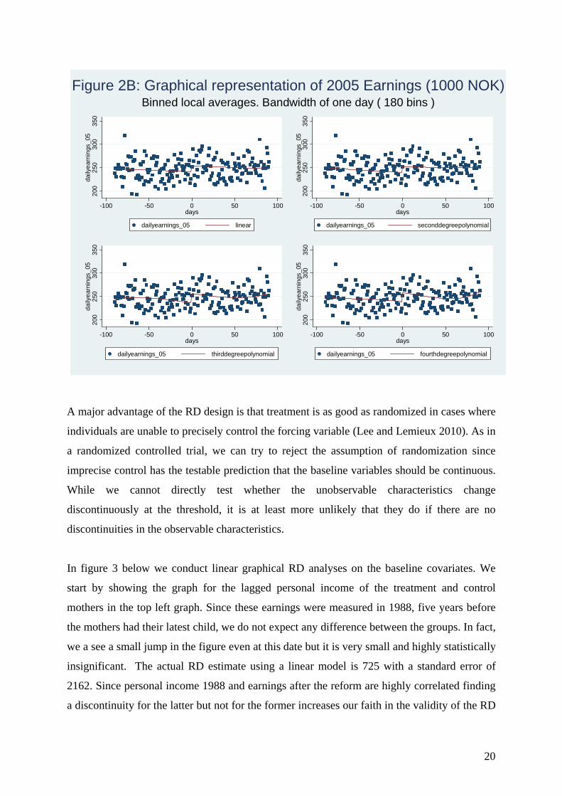
Figures 2A and 2B show the main RD results graphically using binned local averages for
3 The corresponding figures for 1992 can not be used in this respect since there was a reform of the parental leave system April 1st 1992 as well. In fact, we will show the results of that reform in section 6.
19
mean earnings (A) and earnings 2005 (B). The averages are daily unconditional means over
the support of days and as seen in the superimposed regression lines of different polynomial
orders, there is a jump in mean earnings and earnings in 2005 at day 0 (i.e. on April 1st). All
jumps are statistically significant at at least the 10 percent level (more on this in the formal
analysis) and, as can be seen in the figures, the results seem to be robust to different
polynomial specifications.
140
160
180
200
220
mea
near
nin
gsd
ay
-100 -50 0 50 100days
meanearningsday linear
140
160
180
200
220
mea
near
nin
gsd
ay
-100 -50 0 50 100days
meanearningsday seconddegreepolynomial
140
160
180
200
220
mea
near
nin
gsd
ay
-100 -50 0 50 100days
meanearningsday thirddegreepolynomial
140
160
180
200
220
mea
near
nin
gsd
ay
-100 -50 0 50 100days
meanearningsday fourthdegreepolynomial
Binned local averages. Bandwidth of one day ( 180 bins )Figure 2A: Mean earnings between 1995 and 2005 (1000 NOK)
20
200
250
300
350
dai
lye
arni
ngs
_05
-100 -50 0 50 100days
dailyearnings_05 linear
200
250
300
350
dai
lye
arni
ngs
_05
-100 -50 0 50 100days
dailyearnings_05 seconddegreepolynomial
200
250
300
350
dai
lye
arni
ngs
_05
-100 -50 0 50 100days
dailyearnings_05 thirddegreepolynomial
200
250
300
350
dai
lye
arni
ngs
_05
-100 -50 0 50 100days
dailyearnings_05 fourthdegreepolynomial
Binned local averages. Bandwidth of one day ( 180 bins )Figure 2B: Graphical representation of 2005 Earnings (1000 NOK)
A major advantage of the RD design is that treatment is as good as randomized in cases where
individuals are unable to precisely control the forcing variable (Lee and Lemieux 2010). As in
a randomized controlled trial, we can try to reject the assumption of randomization since
imprecise control has the testable prediction that the baseline variables should be continuous.
While we cannot directly test whether the unobservable characteristics change
discontinuously at the threshold, it is at least more unlikely that they do if there are no
discontinuities in the observable characteristics.
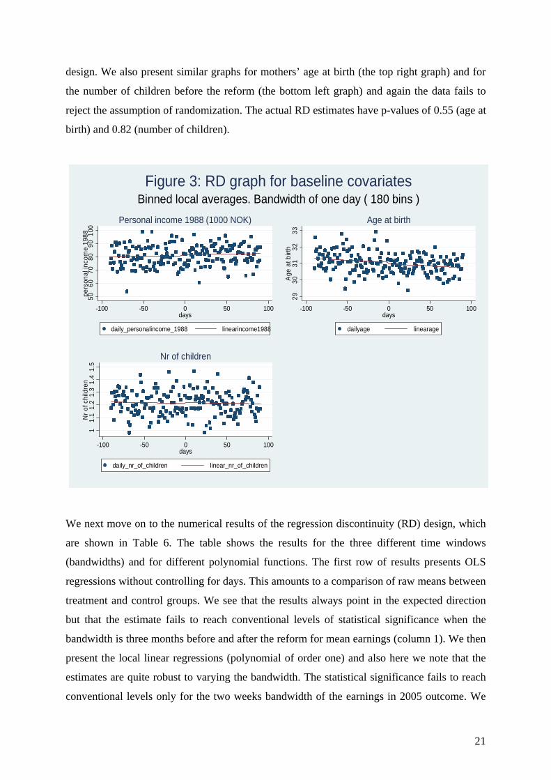
In figure 3 below we conduct linear graphical RD analyses on the baseline covariates. We
start by showing the graph for the lagged personal income of the treatment and control
mothers in the top left graph. Since these earnings were measured in 1988, five years before
the mothers had their latest child, we do not expect any difference between the groups. In fact,
we a see a small jump in the figure even at this date but it is very small and highly statistically
insignificant. The actual RD estimate using a linear model is 725 with a standard error of
2162. Since personal income 1988 and earnings after the reform are highly correlated finding
a discontinuity for the latter but not for the former increases our faith in the validity of the RD
21
design. We also present similar graphs for mothers’ age at birth (the top right graph) and for
the number of children before the reform (the bottom left graph) and again the data fails to
reject the assumption of randomization. The actual RD estimates have p-values of 0.55 (age at
birth) and 0.82 (number of children).
50
60
70
80
90
100
per
son
al in
com
e 1
988
-100 -50 0 50 100days
daily_personalincome_1988 linearincome1988
Personal income 1988 (1000 NOK)
29
30
31
32
33
Age
at b
irth
-100 -50 0 50 100days
dailyage linearage
Age at birth
11
.11
.21
.31
.41
.5N
r of
ch
ildre
n
-100 -50 0 50 100days
daily_nr_of_children linear_nr_of_children
Nr of children
Binned local averages. Bandwidth of one day ( 180 bins )Figure 3: RD graph for baseline covariates
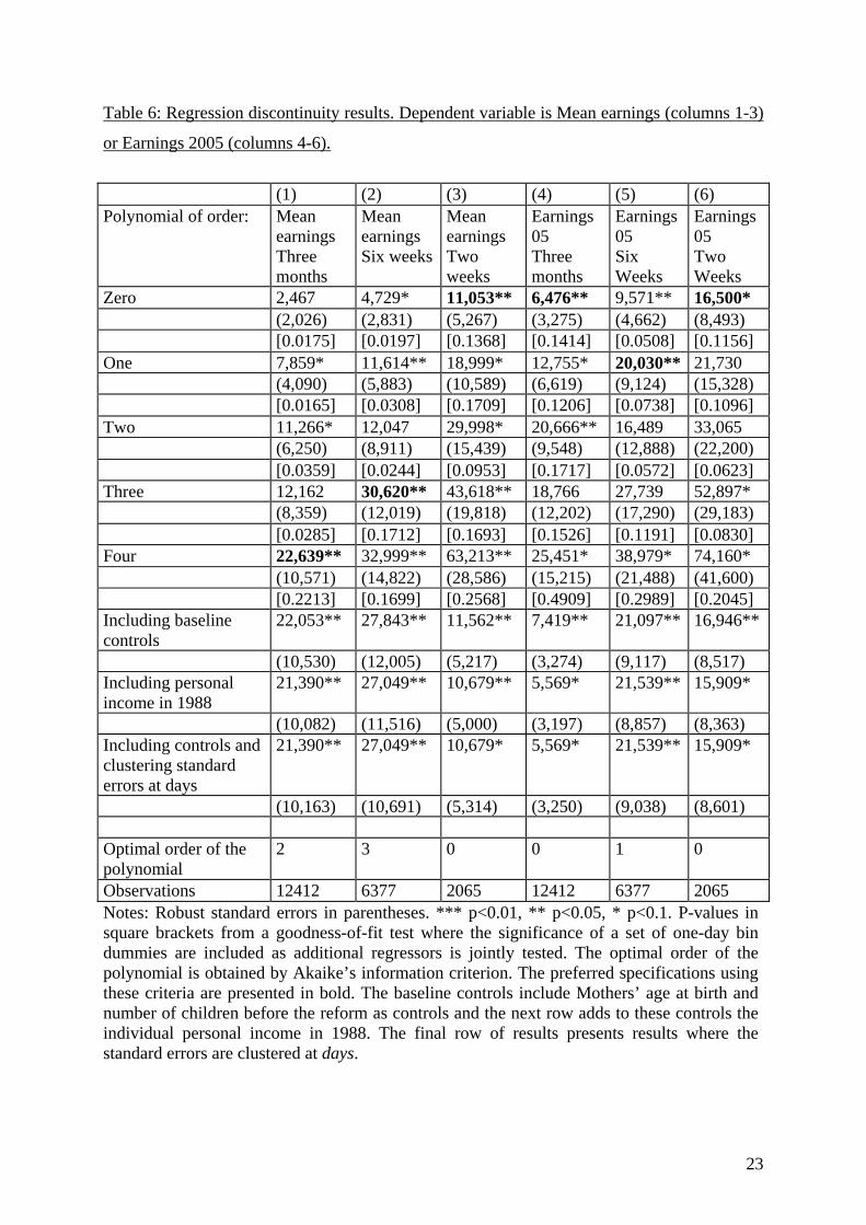
We next move on to the numerical results of the regression discontinuity (RD) design, which
are shown in Table 6. The table shows the results for the three different time windows
(bandwidths) and for different polynomial functions. The first row of results presents OLS
regressions without controlling for days. This amounts to a comparison of raw means between
treatment and control groups. We see that the results always point in the expected direction
but that the estimate fails to reach conventional levels of statistical significance when the
bandwidth is three months before and after the reform for mean earnings (column 1). We then
present the local linear regressions (polynomial of order one) and also here we note that the
estimates are quite robust to varying the bandwidth. The statistical significance fails to reach
conventional levels only for the two weeks bandwidth of the earnings in 2005 outcome. We

22
then proceed and add higher order polynomials to the regression functions in order to assess
the robustness of the results. Our preferred specifications are shown in bold and two test
results guide us in this choice. The first test is a goodness-of-fit test where the significance of
a set of one-day bin dummies are included as additional regressors in the models and p-values
of joint tests of statistical significance of these bin dummies are presented in square brackets.
The decision rule is to add a higher order term to the polynomial until the bin dummies are no
longer jointly significant (Lee and Lemieux 2010). Alternatively, we can use the Akaike
information criterion (AIC) of model selection which rewards goodness of fit but also
penalizes overfitting. The preferred model according to this test is the one with the lowest
AIC value and this is presented in the penultimate row of the table (optimal order of the
polynomial). When the two tests do not allow us to reach the same conclusion, as happens in
column 1, we give priority to the first test. That is, if the function with the optimal order of the
polynomial also passes the goodness of fit test it is preferred, otherwise we add polynomials
until the first test is passed.
The sensitivity of the RD results can also be assessed by inclusion of baseline covariates, and
we see that adding age at the time of birth and number of children before 1993 does not alter
the discontinuity results of the preferred models. This is interpreted as yet a test of that the
observable characteristics are distributed smoothly around the threshold and raises our
confidence in the no manipulation assumption. Next, we add personal income in 1988 as an
additional regressor and note that the results are robust to this inclusion as well. Finally, Lee
and Card (2008) suggest that when the forcing variable is discrete, a parametric approach with
clustered standard errors is preferred to reflect the imperfect fit of the function away from the
threshold. Our forcing variable, days, is indeed discrete and therefore we also run a regression
including baseline control variables (including also personal income in 1988) and cluster the
standard errors at days (cf. Dobkin and Ferreira 2010 who also use daily age as the forcing
variable in identifying the effects of school entry laws). Comparing the standard errors to
those of the previous model without clustered standard errors, we see that they are similar.
23
Table 6: Regression discontinuity results. Dependent variable is Mean earnings (columns 1-3)
or Earnings 2005 (columns 4-6).
(1) (2) (3) (4) (5) (6) Polynomial of order: Mean
earnings Three months
Mean earnings Six weeks
Mean earnings Two weeks
Earnings 05 Three months
Earnings 05 Six Weeks
Earnings 05 Two Weeks
Zero 2,467 4,729* 11,053** 6,476** 9,571** 16,500* (2,026) (2,831) (5,267) (3,275) (4,662) (8,493) [0.0175] [0.0197] [0.1368] [0.1414] [0.0508] [0.1156] One 7,859* 11,614** 18,999* 12,755* 20,030** 21,730 (4,090) (5,883) (10,589) (6,619) (9,124) (15,328) [0.0165] [0.0308] [0.1709] [0.1206] [0.0738] [0.1096] Two 11,266* 12,047 29,998* 20,666** 16,489 33,065 (6,250) (8,911) (15,439) (9,548) (12,888) (22,200) [0.0359] [0.0244] [0.0953] [0.1717] [0.0572] [0.0623] Three 12,162 30,620** 43,618** 18,766 27,739 52,897* (8,359) (12,019) (19,818) (12,202) (17,290) (29,183) [0.0285] [0.1712] [0.1693] [0.1526] [0.1191] [0.0830] Four 22,639** 32,999** 63,213** 25,451* 38,979* 74,160* (10,571) (14,822) (28,586) (15,215) (21,488) (41,600) [0.2213] [0.1699] [0.2568] [0.4909] [0.2989] [0.2045] Including baseline controls
22,053** 27,843** 11,562** 7,419** 21,097** 16,946**
(10,530) (12,005) (5,217) (3,274) (9,117) (8,517) Including personal income in 1988
21,390** 27,049** 10,679** 5,569* 21,539** 15,909*
(10,082) (11,516) (5,000) (3,197) (8,857) (8,363) Including controls and clustering standard errors at days
21,390** 27,049** 10,679* 5,569* 21,539** 15,909*
(10,163) (10,691) (5,314) (3,250) (9,038) (8,601) Optimal order of the polynomial
2 3 0 0 1 0
Observations 12412 6377 2065 12412 6377 2065 Notes: Robust standard errors in parentheses. *** p<0.01, ** p<0.05, * p<0.1. P-values in square brackets from a goodness-of-fit test where the significance of a set of one-day bin dummies are included as additional regressors is jointly tested. The optimal order of the polynomial is obtained by Akaike’s information criterion. The preferred specifications using these criteria are presented in bold. The baseline controls include Mothers’ age at birth and number of children before the reform as controls and the next row adds to these controls the individual personal income in 1988. The final row of results presents results where the standard errors are clustered at days.

24
6. Discussion and generalization
So far we have shown that the parental leave reform in 1993 had large and robust effects on
mothers’ mean earnings as well as long run yearly earnings. The effects are not subject to
spurious variation due to children’s age and they are robust to a number of different
specifications. But how are we to interpret the effects and the magnitudes? A first issue is that
the reform was composite as it included both a prolongation of the total leave period and a
daddy quota of four weeks. Thereby the models identify the joint effect of these possibly
conflicting mechanisms. A second issue is that parents are not forced to use their rights so we
estimate the intention to treat effect rather than the effect of own and spousal parental leave.
The different identification strategies allow us to measure different effects. The OLS
regressions measure the average treatment effects in the window chosen, while the RD
specification gives us the average treatment effect at days=0. Thereby the effect identified in
the RD model is extremely local, however, the internal validity is higher. If we assume
constant treatment effects, the RD model identifies the average treatment effect. But
generally, we only get the average treatment effect for those at the cutoff. Hence, there may
be issues of external validity. Since, however, our different models yield results of similar
magnitudes, we are more confident in extrapolating the RD and the two weeks results.
6.1. The effects of prolonged parental leave
To shed some light on the distribution of the composite effects of the reform, and thereby to
investigate the role of the different mechanisms at play, we start with an investigation of an
earlier reform that did not include a daddy quota but that raised the duration of the parental
leave. We exploit the fact that on April 1st 1992 the parental leave was extended from 32 to 35
weeks, to identify the independent effect of an increase in the parental leave length. The
results of OLS regressions in a two weeks before and after sample are presented in Table 7.
The results (available upon request) are similar for the RD specification as well. We see that
the 1992 reform had no statistically significant effect on the mean earnings of mothers
(columns 1 and 2), nor on the earnings of mothers in 2005 (columns 3 and 4). This is contrary
to what we should expect if the human capital depreciation mechanism was the driving force
behind mothers’ lower earnings. The extension of the parental leave by three weeks, almost
totally used by mothers, did not seem to impact on long run earnings.
25
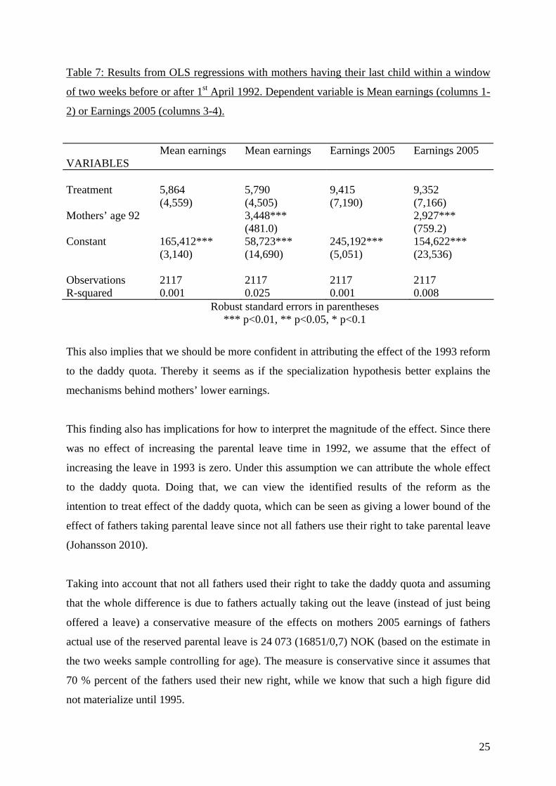
Table 7: Results from OLS regressions with mothers having their last child within a window
of two weeks before or after 1st April 1992. Dependent variable is Mean earnings (columns 1-
2) or Earnings 2005 (columns 3-4).
Mean earnings Mean earnings Earnings 2005 Earnings 2005 VARIABLES Treatment 5,864 5,790 9,415 9,352 (4,559) (4,505) (7,190) (7,166) Mothers’ age 92 3,448*** 2,927*** (481.0) (759.2) Constant 165,412*** 58,723*** 245,192*** 154,622*** (3,140) (14,690) (5,051) (23,536) Observations 2117 2117 2117 2117 R-squared 0.001 0.025 0.001 0.008
Robust standard errors in parentheses *** p<0.01, ** p<0.05, * p<0.1
This also implies that we should be more confident in attributing the effect of the 1993 reform
to the daddy quota. Thereby it seems as if the specialization hypothesis better explains the
mechanisms behind mothers’ lower earnings.
This finding also has implications for how to interpret the magnitude of the effect. Since there
was no effect of increasing the parental leave time in 1992, we assume that the effect of
increasing the leave in 1993 is zero. Under this assumption we can attribute the whole effect
to the daddy quota. Doing that, we can view the identified results of the reform as the
intention to treat effect of the daddy quota, which can be seen as giving a lower bound of the
effect of fathers taking parental leave since not all fathers use their right to take parental leave
(Johansson 2010).
Taking into account that not all fathers used their right to take the daddy quota and assuming
that the whole difference is due to fathers actually taking out the leave (instead of just being
offered a leave) a conservative measure of the effects on mothers 2005 earnings of fathers
actual use of the reserved parental leave is 24 073 (16851/0,7) NOK (based on the estimate in
the two weeks sample controlling for age). The measure is conservative since it assumes that
70 % percent of the fathers used their new right, while we know that such a high figure did
not materialize until 1995.

26
6.2. Variation in the effect of the reform by different birth parities.
So far we have investigated the effect of having a last child immediately after the introduction
of the reform without discriminating between e.g. effects of firstborns or those already having
older children at the reform date. In this section we match mothers of the same birth parity
and run OLS regressions on our “random” (two weeks before and after) sample. Ex-ante it is
not clear what we should expect since there are different mechanisms at play when
investigating the birth parity of mothers. If the firstborn child is most important in setting
durable patterns of household division of labor we should expect greater effects for those with
only one child. If, however, mothers of more children have more to gain from a more equal
sharing of household tasks due to a greater workload we should expect the effects to be
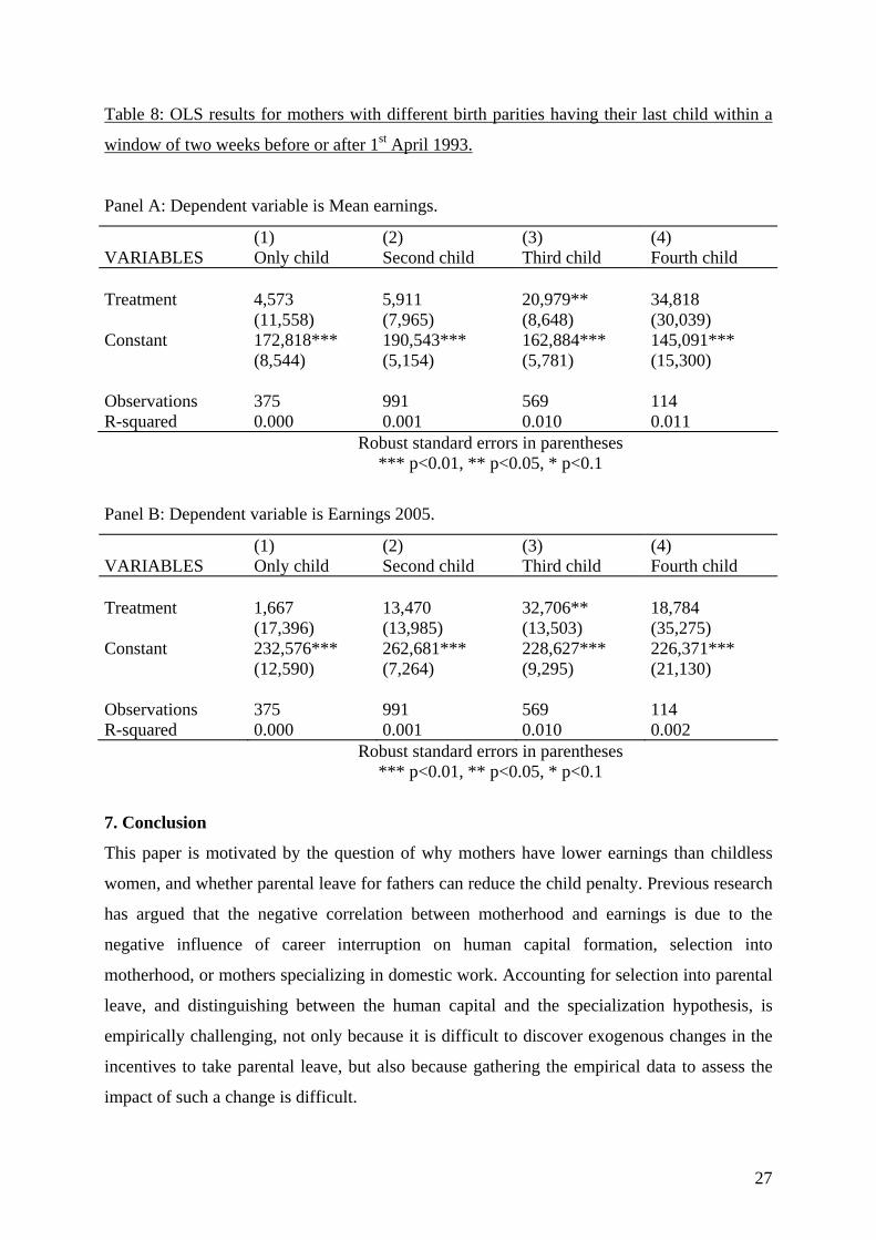
greatest for those with more children before the reform. As seen in Table 8 the coefficient for
the treatment effect is mostly statistically insignificant when broken down by birth parity but
the coefficient rises with the number of children born before the reform, thereby favoring the
second explanation of greater effects of the daddy quota on women’s earnings if the women
already had children from before. That the results differ according to birth parity has
implications for the external validity of our results as we are more likely to include mothers
that already had other children at the time of the reform by focusing on the last born child
(which is necessary for internal validity) than if we would have focused on mothers of any
child born around the reform. This implies that our results may be overestimated as compared
to the average effect of the reform for all parents.
27
Table 8: OLS results for mothers with different birth parities having their last child within a
window of two weeks before or after 1st April 1993.
Panel A: Dependent variable is Mean earnings.
(1) (2) (3) (4) VARIABLES Only child Second child Third child Fourth child Treatment 4,573 5,911 20,979** 34,818 (11,558) (7,965) (8,648) (30,039) Constant 172,818*** 190,543*** 162,884*** 145,091*** (8,544) (5,154) (5,781) (15,300) Observations 375 991 569 114 R-squared 0.000 0.001 0.010 0.011
Robust standard errors in parentheses *** p<0.01, ** p<0.05, * p<0.1
Panel B: Dependent variable is Earnings 2005.
(1) (2) (3) (4) VARIABLES Only child Second child Third child Fourth child Treatment 1,667 13,470 32,706** 18,784 (17,396) (13,985) (13,503) (35,275) Constant 232,576*** 262,681*** 228,627*** 226,371*** (12,590) (7,264) (9,295) (21,130) Observations 375 991 569 114 R-squared 0.000 0.001 0.010 0.002
Robust standard errors in parentheses *** p<0.01, ** p<0.05, * p<0.1
7. Conclusion
This paper is motivated by the question of why mothers have lower earnings than childless
women, and whether parental leave for fathers can reduce the child penalty. Previous research
has argued that the negative correlation between motherhood and earnings is due to the
negative influence of career interruption on human capital formation, selection into
motherhood, or mothers specializing in domestic work. Accounting for selection into parental
leave, and distinguishing between the human capital and the specialization hypothesis, is
empirically challenging, not only because it is difficult to discover exogenous changes in the
incentives to take parental leave, but also because gathering the empirical data to assess the
impact of such a change is difficult.
28
We take advantage of the introduction of a Norwegian parental leave reform which implied
that parents with children born after April 1st 1993 had access to seven additional weeks of
parental leave, of which four weeks were reserved for the father (a so-called daddy quota).
We have access to register data with exact birth dates for children born just before and just
after the reform, and their mothers’ earnings developments over a long period, which allows
us to establish the composite causal effect of the reform on earnings. According to the human
capital depreciation hypothesis, we should expect a negative effect of the reform on mothers’
earnings, since the leave period was extended, while according to the specialization
hypothesis, the effect is likely to be positive as the daddy quota decreases mothers’
specialization into child rearing.
We find that the reform had significant and substantive effects on mothers’ earnings. Both
mean earnings 1995-2005 and yearly earnings in 2005 (which is our last date of data
measurement) of mothers that had her last child after the reform are higher compared to
mothers that had her last child before the reform. Controlling for age differences, this is true
whether we rely on a three months, six weeks, or two weeks time window before and after the
reform. According to the estimates using the two weeks before and after window (where day
of birth is close to random), the reform led to an increase in earnings 2005, i.e. more than 12
years after the reform, by 6.9 percent or of between 158 and 33 545 NOK (approximately
between 26 and 5007 US dollars). Using the same sample criterion and investigating the
effects in other years we see that mothers’ earnings in the treatment group were higher for all
years between 1997 and 2005. The conclusion that the wage difference between the treatment
and control group is due to the reform is robust to several falsification tests, and a regression
discontinuity analysis is also applied showing that mothers of children born immediately after
the reform have higher earnings than mothers of children born immediately before the reform.
These reduced form findings lend support to the specialization hypothesis rather than the
human capital hypothesis, an interpretation that is also strengthened by the insignificant effect
on earnings of a parental leave reform in 1992 which expanded the period of leave, but with
no daddy quota.
The high internal validity of our research design implies that we are confident that the reform
had an effect of mothers’ long run earnings. The results also correspond well with those in
Johansson (2010) for Sweden who find that a month of parental leave for fathers increased

29
mothers’ yearly earnings by 6.7 percent and the results in Lalive and Zweimüller (2009) from
Austria of no effects of own parental leave for mothers’ long run wages. Kluve and Tamm
(2009) do not find a two year effect in Germany and we do not find any statistical difference
between our groups two years after our main reform either which highlights the importance of
investigating longer time periods. Our results do not, however, fit those found for Sweden by
Johansson (2010) with respect to the effects of own leave taking for mothers. Her result of a
negative effect of own parental leave is, however, only found in the less robust fixed effects
specifications. Although our results support the specialization hypothesis and are in line with
the results of decreased household work specialization results found in Norway by Kotsadam
and Finseraas (2010) we are still less confident that we have identified the one and only
mechanism (less female specialization). In particular, we only identify the marginal effects of
increasing the parental leave by three weeks (in the 1992 reform) and the joint effect of
increasing the parental leave with three weeks and adding a fathers quota of four weeks (in
the 1993 reform). These marginal effects most likely differ considerably from more radical
reforms and to reforms conducted with different starting levels. We urge further research to
explore these issues more in depth.
30
References
Albrecht, J. Per-Anders Edin, P-A., Sundström, M., and Vroman S (1999) “Career
Interruptions and Subsequent Earnings: A Reexamination Using Swedish Data” The
Journal of Human Resources Vol. 34, No. 2, pp. 294-311
Angrist, Joshua D. and Jörn-Steffen Pischke (2008). Mostly Harmless Econometrics: An
Empiricist’s Companion, Princeton: Princeton University Press.
Bruning, G. and Plantenga, J. (1999) ‘Parental Leave and Equal Opportunities Experiences in
Eight European Countries’ Journal of European Social Policy 9 (3) 195-209.
Buckles, Kasey, and Daniel M. Hungerman. 2008. "Season of Birth and later outcomes: old
questions, new answers." NBER Working Paper No. 14 573.
Dobkin C. and Ferreira F. (2010). ”Do school entry laws affect educational attainment and
labor market outcomes?” Economics of Education Review, Vol. 29, pp. 40-54.
Ekberg J., Eriksson, R. and Friebel, G. (2006) “Parental Leave – A Policy Evaluation of the
Swedish “Daddy-Month” Reform” IZA Discussion Paper No. 1617.
Eriksson, R. (2005), Parental leave in Sweden: The effects of the second daddy month”
Stockholm University Working Paper No. 9 2005.
European Union (2010), “Council Directive 2010/18/EU of 8 March 2010 implementing the
revised Framework Agreement on parental leave.”
Hernes, H. (1987), Welfare State and Woman Power. Essays in State Feminism.
Universitetsforlaget, Oslo.
Hook, J. L. (2010), “Gender Inequality in the Welfare State: Sex Segregation in Housework,
1965-2003”, American Journal of Sociology Vol. 115, No. 5, pp. 1480-1523.
Johansson, E-A. (2010), “The effect of own and spousal parental leave on earnings”, IFAU
Working Paper 2010:4.
Kluve, J. and Tamm, M. (2009), “Now Daddy's Changing Diapers and Mommy's Making Her
Career-Evaluating a Generous Parental Leave Regulation Using a Natural Experiment”
IZA Discussion paper No. 4500.
Lalive, R. and Zweimüller, J. (2009), ”How does Parental Leave Affect Fertility and Return to
Work? Evidence from Two Natural Experiments”, Quarterly Journal of Economics, Vol.
124, No. 3, pp. 1363-1402
Lee, D. and Lemieux, T. (2010), ”Regression Discontinuty Designs in Economics”, Journal of Economic Litterature, 48, pp. 281-355.
Lee D. and D. Card (2008). ”Regression discontinuity with specification error.” Journal of
Econometrics, vol. 142, pp. 655-674.
31
Leira, Arnlaug (1998) “Caring as a Social Right: Cash for Childcare and Daddy Leave.”
Social Politics 5: 362-378.
Leira, A (2002) Working parents and the Welfare State. Family Change and Policy Reforms
in Scandinavia. Cambridge University Press.
Lundberg, S. and Rose, E. (2000) “Parenthood and the Earnings of Married Men and
Women”, Labour Economics, 7 (6), p. 689-710
McCrary, J. (2008). “Manipulation of the Running Variable in the Regression Discontinuity
Design: A Density Test”, Journal of Econometrics, 142, pp. 698-714.
Mincer, J. and Polachek, S. (1974), “Family Investments in Human Capital: Earnings of
Women” NBER Chapters in Marriage, Family, Human Capital, and Fertility, pages 76-
110 National Bureau of Economic Research, Inc.
Nielsen, H., (2009), “Causes and Consequences of a Father´s Child Leave: Evidence from a
Reform of Leave Schemes” IZA Discussion paper No. 4267.
NOU (1995), Pappa kom hjem. Norges offentlige utredninger. 1995:27 NOU (1996), Offentlige overføringer til barnefamilier. Norges offentlige utredninger.
1996:13 Rege, M. and Solli, I. (2010), “The Impact of Paternity Leave on Long-term Father
Involvement” CESIFO Working Paper No. 3130.
Rosenzweig, M and Wolpin, K. 2000. " Natural "Natural Experiments" in Economics"
Journal of Economic Literature, vol. 38(4), pp. 827-874.
Ruhm, C. (1998), “The economic Consequences of Parental leave Mandates: Lessons from
Europe”, The Quarterly Journal of Economics, Vol. 13, No. 1, pp. 285-317.

32
Appendix:
Table A1: OLS regressions on Mean earnings (Panel A) and Earnings 2005 (Panel B) with
shorter time windows. Mothers having there last child one day, three days, and one week
before and after the introduction of the reform are compared.
Panel A: Dependent variable is Mean earnings.
(1) (2) (3) VARIABLES one day three days one week Treatment 26,199 30,844** 13,903* (16,550) (12,123) (7,280) Constant 159,884*** 165,197*** 172,965*** (10,723) (7,777) (5,218) Observations 165 424 1020 R-squared 0.015 0.015 0.004
Robust standard errors in parentheses *** p<0.01, ** p<0.05, * p<0.1
Panel B: Dependent variable is Earnings 2005.
(1) (2) (3) VARIABLES one day three days one week Treatment 27,176 35,644** 15,708 (25,074) (17,120) (10,237) Constant 225,025*** 232,391*** 239,946*** (16,886) (12,681) (7,491) Observations 165 424 1020 R-squared 0.007 0.010 0.002
Robust standard errors in parentheses *** p<0.01, ** p<0.05, * p<0.1