Embed Size (px)
Citation preview
The Long Bond
Ian Martin (Stanford)
Steve Ross (MIT)
August, 2013
Martin, Ross (Stanford, MIT) The Long Bond August, 2013 1 / 38
Outline
A simple framework for thinking about the properties of the long
end of the yield curve
Connects the “Recovery Theorem” of Ross (2013) to earlier work
of Backus, Gregory and Zin (1989), Kazemi (1992), Bansal and
Lehmann (1997), Alvarez and Jermann (2005) and Hansen and
Scheinkman (2009)
Martin, Ross (Stanford, MIT) The Long Bond August, 2013 2 / 38
Outline
What do we learn by observing the (infinitely) long yield?
What do we learn by observing the realized returns on the
(infinitely) long bond?
What shape is the yield curve, on average?
What information can we learn from interest-rate options?
What is the expected return on the long bond?
Martin, Ross (Stanford, MIT) The Long Bond August, 2013 3 / 38
The framework
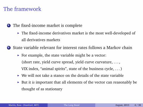
1 The fixed-income market is complete
I The fixed-income derivatives market is the most well-developed of
all derivatives markets
2 State variable relevant for interest rates follows a Markov chain
I For example, the state variable might be a vector:
(short rate, yield curve spread, yield curve curvature, . . . ,
VIX index, “animal spirits”, state of the business cycle, . . . )
I We will not take a stance on the details of the state variable
I But it is important that all elements of the vector can reasonably be
thought of as stationary
Martin, Ross (Stanford, MIT) The Long Bond August, 2013 4 / 38
The framework
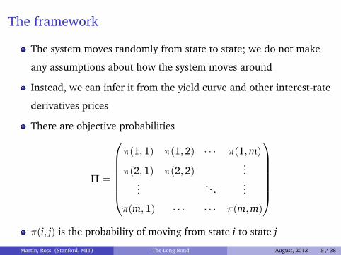
The system moves randomly from state to state; we do not make
any assumptions about how the system moves around
Instead, we can infer it from the yield curve and other interest-rate
derivatives prices
There are objective probabilities
Π =
π(1,1) π(1,2) · · · π(1,m)
π(2,1) π(2,2)...
.... . .
...
π(m,1) · · · · · · π(m,m)
π(i, j) is the probability of moving from state i to state j
Martin, Ross (Stanford, MIT) The Long Bond August, 2013 5 / 38
The framework
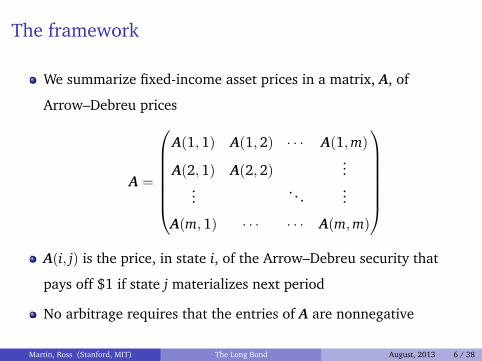
We summarize fixed-income asset prices in a matrix, A, of
Arrow–Debreu prices
A =
A(1,1) A(1,2) · · · A(1,m)
A(2,1) A(2,2)...
.... . .
...
A(m,1) · · · · · · A(m,m)
A(i, j) is the price, in state i, of the Arrow–Debreu security that
pays off $1 if state j materializes next period
No arbitrage requires that the entries of A are nonnegative
Martin, Ross (Stanford, MIT) The Long Bond August, 2013 6 / 38
The framework
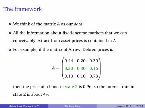
We think of the matrix A as our data
All the information about fixed-income markets that we can
conceivably extract from asset prices is contained in A
For example, if the matrix of Arrow–Debreu prices is
A =
0.44 0.20 0.30
0.50 0.30 0.16
0.10 0.10 0.78
then the price of a bond in state 2 is 0.96, so the interest rate in
state 2 is about 4%
Martin, Ross (Stanford, MIT) The Long Bond August, 2013 7 / 38
Recovery
Assume (for now) that A is directly observable
What can we learn from A?
In particular, can we learn the transition probabilities?
In the finance lingo, asset prices tell us Q; but can we learn P?
Martin, Ross (Stanford, MIT) The Long Bond August, 2013 8 / 38
Recovery
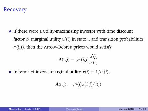
If there were a utility-maximizing investor with time discount
factor φ, marginal utility u′(i) in state i, and transition probabilities
π(i, j), then the Arrow–Debreu prices would satisfy
A(i, j) = φπ(i, j)u′(j)u′(i)
In terms of inverse marginal utility, v(i) ≡ 1/u′(i),
A(i, j) = φv(i)π(i, j)/v(j)
Martin, Ross (Stanford, MIT) The Long Bond August, 2013 9 / 38
Recovery
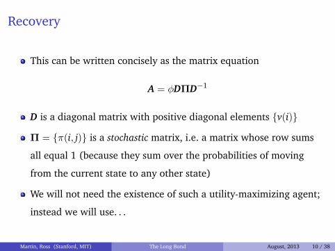
This can be written concisely as the matrix equation
A = φDΠD−1
D is a diagonal matrix with positive diagonal elements {v(i)}
Π = {π(i, j)} is a stochastic matrix, i.e. a matrix whose row sums
all equal 1 (because they sum over the probabilities of moving
from the current state to any other state)
We will not need the existence of such a utility-maximizing agent;
instead we will use. . .
Martin, Ross (Stanford, MIT) The Long Bond August, 2013 10 / 38
The pseudo-representative agent
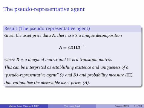
Result (The pseudo-representative agent)Given the asset price data A, there exists a unique decomposition
A = φDΠD−1
where D is a diagonal matrix and Π is a transition matrix.
This can be interpreted as establishing existence and uniqueness of a
“pseudo-representative agent” (φ and D) and probability measure (Π)
that rationalize the observable asset prices (A).
Martin, Ross (Stanford, MIT) The Long Bond August, 2013 11 / 38
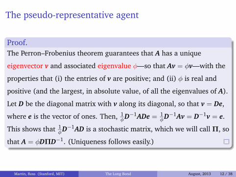
The pseudo-representative agent
Proof.The Perron–Frobenius theorem guarantees that A has a unique
eigenvector v and associated eigenvalue φ—so that Av = φv—with the
properties that (i) the entries of v are positive; and (ii) φ is real and
positive (and the largest, in absolute value, of all the eigenvalues of A).
Let D be the diagonal matrix with v along its diagonal, so that v = De,
where e is the vector of ones. Then, 1φD−1ADe = 1
φD−1Av = D−1v = e.
This shows that 1φD−1AD is a stochastic matrix, which we will call Π, so
that A = φDΠD−1. (Uniqueness follows easily.)
Martin, Ross (Stanford, MIT) The Long Bond August, 2013 12 / 38
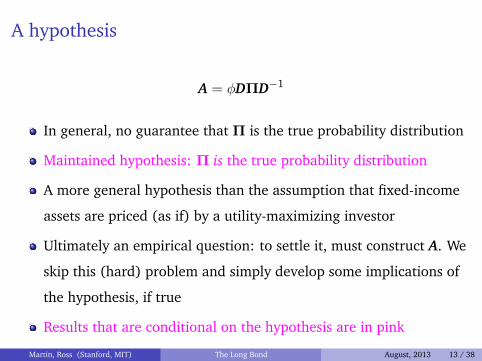
A hypothesis
A = φDΠD−1
In general, no guarantee that Π is the true probability distribution
Maintained hypothesis: Π is the true probability distribution
A more general hypothesis than the assumption that fixed-income
assets are priced (as if) by a utility-maximizing investor
Ultimately an empirical question: to settle it, must construct A. We
skip this (hard) problem and simply develop some implications of
the hypothesis, if true
Results that are conditional on the hypothesis are in pink
Martin, Ross (Stanford, MIT) The Long Bond August, 2013 13 / 38
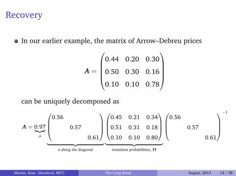
Recovery
In our earlier example, the matrix of Arrow–Debreu prices
A =
0.44 0.20 0.30
0.50 0.30 0.16
0.10 0.10 0.78
can be uniquely decomposed as
A = 0.97︸︷︷︸φ
0.56
0.57
0.61
︸ ︷︷ ︸
v along the diagonal
0.45 0.21 0.34
0.51 0.31 0.18
0.10 0.10 0.80
︸ ︷︷ ︸
transition probabilities, Π
0.56
0.57
0.61
−1
Martin, Ross (Stanford, MIT) The Long Bond August, 2013 14 / 38
Recovery
The eigenvector v represents the vector of (inverse) marginal
utilities across states
The eigenvalue φ represents the pure time discount factor
We can use these, together with A, to calculate the transition
probability matrix Π
But it may be hard, in practice, to calculate the original matrix A
We need to observe the yield curve and prices of a rich range of
interest-rate derivatives—swaptions, caps, floors, . . .
Martin, Ross (Stanford, MIT) The Long Bond August, 2013 15 / 38
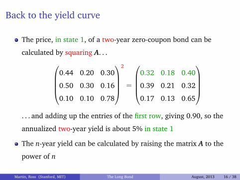
Back to the yield curve
The price, in state 1, of a two-year zero-coupon bond can be
calculated by squaring A. . .0.44 0.20 0.30
0.50 0.30 0.16
0.10 0.10 0.78
2
=
0.32 0.18 0.40
0.39 0.21 0.32
0.17 0.13 0.65
. . . and adding up the entries of the first row, giving 0.90, so the
annualized two-year yield is about 5% in state 1
The n-year yield can be calculated by raising the matrix A to the
power of n
Martin, Ross (Stanford, MIT) The Long Bond August, 2013 16 / 38
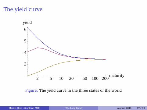
The yield curve
2 5 10 20 50 100 200maturity
3
4
5
6
yield
Figure: The yield curve in the three states of the world
Martin, Ross (Stanford, MIT) The Long Bond August, 2013 17 / 38
The yield curve
Result (The long bond yield reveals φ)The yield and unconditional expected log return of the long bond are
determined by φ, the largest eigenvalue of A: y∞ = r∞ = − logφ.
The long bond: the infinitely long zero-coupon bond
So, in our setting, the long end of the yield curve directly reveals
the time discount factor of the pseudo-representative agent
No need to compute A
The long yield is constant (cf Dybvig, Ingersoll and Ross 1996)
Martin, Ross (Stanford, MIT) The Long Bond August, 2013 18 / 38
The yield curve
We now have a direct link between the eigenvalue and something
we can observe in the market
Want to do the same for the eigenvector, v, which summarizes
marginal utilities across states
Idea: interpret v as the payoffs on an asset that pays v(1) in state
1, v(2) in state 2, . . .
This asset has a nice interpretation
Martin, Ross (Stanford, MIT) The Long Bond August, 2013 19 / 38
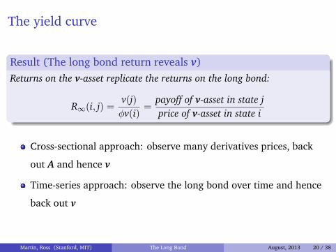
The yield curve
Result (The long bond return reveals v)Returns on the v-asset replicate the returns on the long bond:
R∞(i, j) =v(j)φv(i)
=payoff of v-asset in state jprice of v-asset in state i
Cross-sectional approach: observe many derivatives prices, back
out A and hence v
Time-series approach: observe the long bond over time and hence
back out v
Martin, Ross (Stanford, MIT) The Long Bond August, 2013 20 / 38
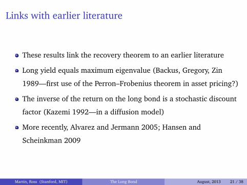
Links with earlier literature
These results link the recovery theorem to an earlier literature
Long yield equals maximum eigenvalue (Backus, Gregory, Zin
1989—first use of the Perron–Frobenius theorem in asset pricing?)
The inverse of the return on the long bond is a stochastic discount
factor (Kazemi 1992—in a diffusion model)
More recently, Alvarez and Jermann 2005; Hansen and
Scheinkman 2009
Martin, Ross (Stanford, MIT) The Long Bond August, 2013 21 / 38
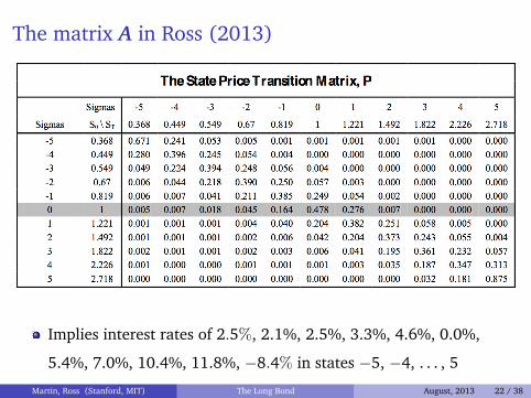
The matrix A in Ross (2013)
Implies interest rates of 2.5%, 2.1%, 2.5%, 3.3%, 4.6%, 0.0%,
5.4%, 7.0%, 10.4%, 11.8%, −8.4% in states −5, −4, . . . , 5
Martin, Ross (Stanford, MIT) The Long Bond August, 2013 22 / 38
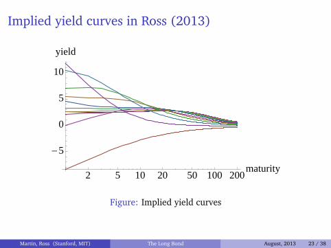
Implied yield curves in Ross (2013)
2 5 10 20 50 100 200maturity
-5
0
5
10
yield
Figure: Implied yield curves
Martin, Ross (Stanford, MIT) The Long Bond August, 2013 23 / 38
Comparison with Ross (2013)
If the riskless rate is constant, pricing is risk-neutral
Confronted with high risk premia in equity markets, the
framework is forced to conclude that the riskless rate varies wildly
Martin, Ross (Stanford, MIT) The Long Bond August, 2013 24 / 38
Long and not-so-long bonds
The long bond is a theoretically appealing construct. But how
closely it can be approximated by bonds of finite maturity?
Introduce the quantity
Q ≡ logmaxk v(k)mink v(k)
Q indexes the importance of risk for bond pricing
Maximum and minimum possible log returns on the long bond are
mini,j
r∞(i, j) = y∞ − Q and maxi,j
r∞(i, j) = y∞ + Q
Martin, Ross (Stanford, MIT) The Long Bond August, 2013 25 / 38
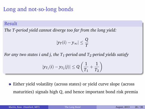
Long and not-so-long bonds
ResultThe T-period yield cannot diverge too far from the long yield:
|yT(i)− y∞| ≤QT
For any two states i and j, the T1-period and T2-period yields satisfy
|yT1(i)− yT2(j)| ≤ Q(
1T1
+1T2
)
Either yield volatility (across states) or yield curve slope (across
maturities) signals high Q, and hence important bond risk premia
Martin, Ross (Stanford, MIT) The Long Bond August, 2013 26 / 38
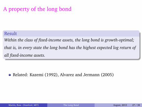
A property of the long bond
ResultWithin the class of fixed-income assets, the long bond is growth-optimal;
that is, in every state the long bond has the highest expected log return of
all fixed-income assets.
Related: Kazemi (1992), Alvarez and Jermann (2005)
Martin, Ross (Stanford, MIT) The Long Bond August, 2013 27 / 38
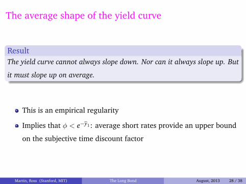
The average shape of the yield curve
ResultThe yield curve cannot always slope down. Nor can it always slope up. But
it must slope up on average.
This is an empirical regularity
Implies that φ < e−y1: average short rates provide an upper bound
on the subjective time discount factor
Martin, Ross (Stanford, MIT) The Long Bond August, 2013 28 / 38
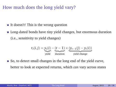
How much does the long yield vary?
It doesn’t! This is the wrong question
Long-dated bonds have tiny yield changes, but enormous duration
(i.e., sensitivity to yield changes)
rt(i, j) = yt(i)︸︷︷︸yield
− (t− 1)︸ ︷︷ ︸duration
× (yt−1(j)− yt(i))︸ ︷︷ ︸yield change
So, to detect small changes in the long end of the yield curve,
better to look at expected returns, which can vary across states
Martin, Ross (Stanford, MIT) The Long Bond August, 2013 29 / 38
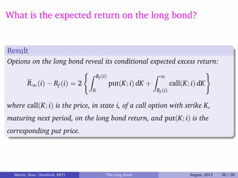
What is the expected return on the long bond?
ResultOptions on the long bond reveal its conditional expected excess return:
R∞(i)− Rf (i) = 2
{∫ Rf (i)
0put(K; i) dK +
∫ ∞Rf (i)
call(K; i) dK
}
where call(K; i) is the price, in state i, of a call option with strike K,
maturing next period, on the long bond return, and put(K; i) is the
corresponding put price.
Martin, Ross (Stanford, MIT) The Long Bond August, 2013 30 / 38
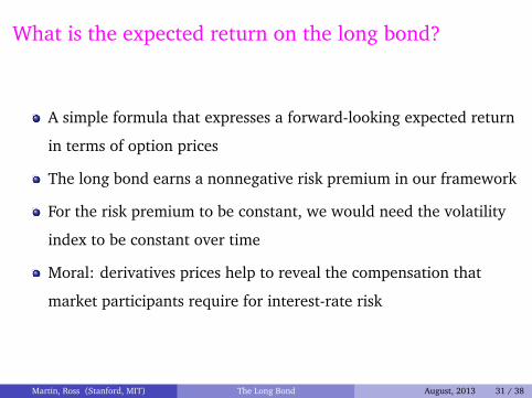
What is the expected return on the long bond?
A simple formula that expresses a forward-looking expected return
in terms of option prices
The long bond earns a nonnegative risk premium in our framework
For the risk premium to be constant, we would need the volatility
index to be constant over time
Moral: derivatives prices help to reveal the compensation that
market participants require for interest-rate risk
Martin, Ross (Stanford, MIT) The Long Bond August, 2013 31 / 38
What’s going on?
In one respect our assumptions are very weak: we do not even
assume that the concept of utility is well-defined
There may be very rare and unpleasant states of the world
Nonetheless, interest rates are stationary and bounded
These properties are not satisfied in other models, which can have
yield curves that are downward-sloping on average (eg, Vasicek,
Cox–Ingersoll–Ross, Bansal–Yaron, Gollier, . . . )
Martin, Ross (Stanford, MIT) The Long Bond August, 2013 32 / 38
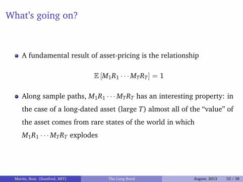
What’s going on?
A fundamental result of asset-pricing is the relationship
E [M1R1 · · ·MTRT] = 1
Along sample paths, M1R1 · · ·MTRT has an interesting property: in
the case of a long-dated asset (large T) almost all of the “value” of
the asset comes from rare states of the world in which
M1R1 · · ·MTRT explodes
Martin, Ross (Stanford, MIT) The Long Bond August, 2013 33 / 38

Figure: 400 sample paths of M1R1 · · ·MTRT over a 250-year horizon
Martin, Ross (Stanford, MIT) The Long Bond August, 2013 34 / 38
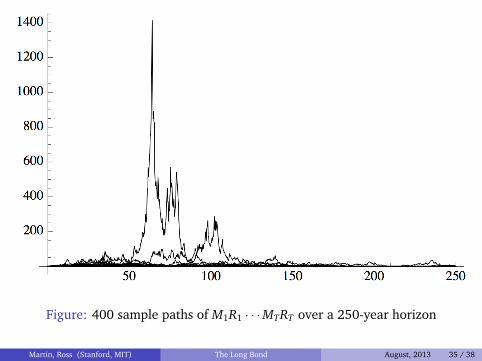
Figure: 400 sample paths of M1R1 · · ·MTRT over a 250-year horizon
Martin, Ross (Stanford, MIT) The Long Bond August, 2013 35 / 38
What’s going on?
Whether or not the economy features disasters in the Rietz–Barro
sense, extreme outcomes matter for pricing long-dated assets
This is true for all assets except the growth-optimal asset
But, in our setting, the long bond is growth-optimal, so it is the
unique fixed-income asset that can escape this conclusion
Martin, Ross (Stanford, MIT) The Long Bond August, 2013 36 / 38
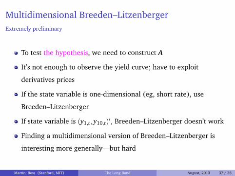
Multidimensional Breeden–LitzenbergerExtremely preliminary
To test the hypothesis, we need to construct A
It’s not enough to observe the yield curve; have to exploit
derivatives prices
If the state variable is one-dimensional (eg, short rate), use
Breeden–Litzenberger
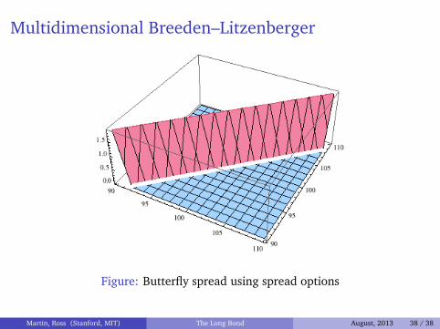
If state variable is (y1,t, y10,t)′, Breeden–Litzenberger doesn’t work
Finding a multidimensional version of Breeden–Litzenberger is
interesting more generally—but hard
Martin, Ross (Stanford, MIT) The Long Bond August, 2013 37 / 38
Multidimensional Breeden–Litzenberger
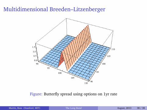
Figure: Butterfly spread using options on 1yr rate
Martin, Ross (Stanford, MIT) The Long Bond August, 2013 38 / 38
Multidimensional Breeden–Litzenberger
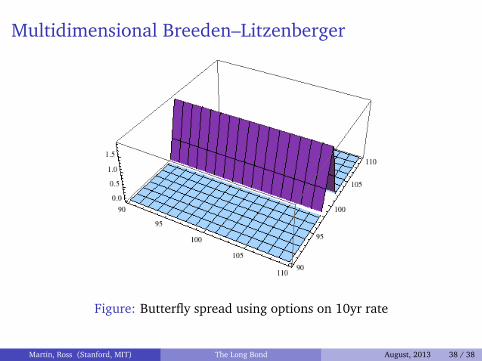
Figure: Butterfly spread using options on 10yr rate
Martin, Ross (Stanford, MIT) The Long Bond August, 2013 38 / 38
Multidimensional Breeden–Litzenberger
Figure: Butterfly spread using spread options
Martin, Ross (Stanford, MIT) The Long Bond August, 2013 38 / 38
Multidimensional Breeden–Litzenberger
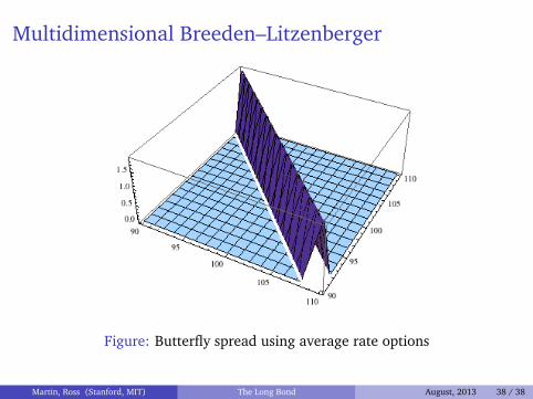
Figure: Butterfly spread using average rate options
Martin, Ross (Stanford, MIT) The Long Bond August, 2013 38 / 38
Multidimensional Breeden–Litzenberger
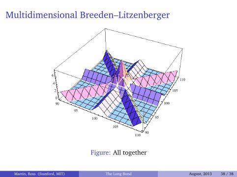
Figure: All together
Martin, Ross (Stanford, MIT) The Long Bond August, 2013 38 / 38

Multidimensional Breeden–Litzenberger
Figure: All together
Martin, Ross (Stanford, MIT) The Long Bond August, 2013 38 / 38