Embed Size (px)
Citation preview
The Logic of an EPP experiment Go back to Rutherford and the logical steps of his experiment (slide 8)
15/10/17 Experimental Elementary Particle Physics 45
“Logic” of an EPP experiment - I
15/10/17 Experimental Elementary Particle Physics 46
� Collision or decay: è process to look at � Initial state (proj. + target) OR (decaying particle); � Final state X = all particles produced
� Quadri-momentum conservation should always be at work � In principle there is no need to measure ALL final state particles: a
final state could be: à µ+µ- + X (“inclusive” search) � Possible final states:
� a + b à a + b : elastic collision (e.g. ppà pp) � a + b à X : inelastic collision (e.g. ppàppπ0)
� The experimentalist should set-up an experimental procedure to select the final state he/she searches. First of all he should be able to count the number NX of final states X.
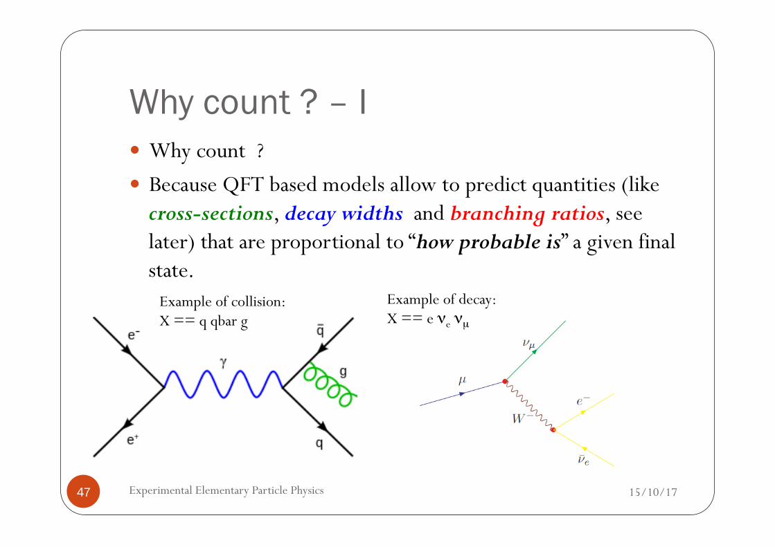
Why count ? – I
15/10/17 Experimental Elementary Particle Physics 47
� Why count ? � Because QFT based models allow to predict quantities (like
cross-sections, decay widths and branching ratios, see later) that are proportional to “how probable is” a given final state.
Example of collision: X == q qbar g
Example of decay: X == e νe νµ
Why count ? – II
15/10/17 Experimental Elementary Particle Physics 48
� Given a collision or a decaying particle you have several possibilities, several different final states.
� So: if I have produced N initial states (either a+b collisions or decaying particles), and out of them n times I observe the final state I am looking for, I can access this probability that should be ≈ n/N
� Let me introduce the concept of Event: � The collection of all the particles of the final state from a single
collision. � It is a collection of particles with their quadri-momenta. � Be careful not to overlap particles from different collisions.
Binomial or Poissonian ?
15/10/17 Experimental Elementary Particle Physics 49
� N initial states prepared n final states observed à inference on p. So binomial ? Yes BUT:
� N is not known exactly � If N à ∞ and p à 0 è n follows a poissonian
distribution (easy to prove)
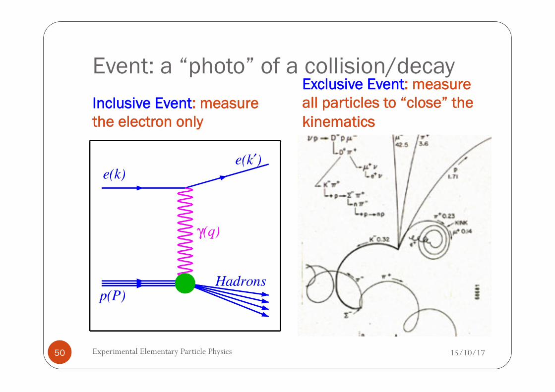
Event: a “photo” of a collision/decay Inclusive Event: measure the electron only
Exclusive Event: measure all particles to “close” the kinematics
15/10/17 Experimental Elementary Particle Physics 50
“Logic” of an EPP experiment - II
15/10/17 Experimental Elementary Particle Physics 51
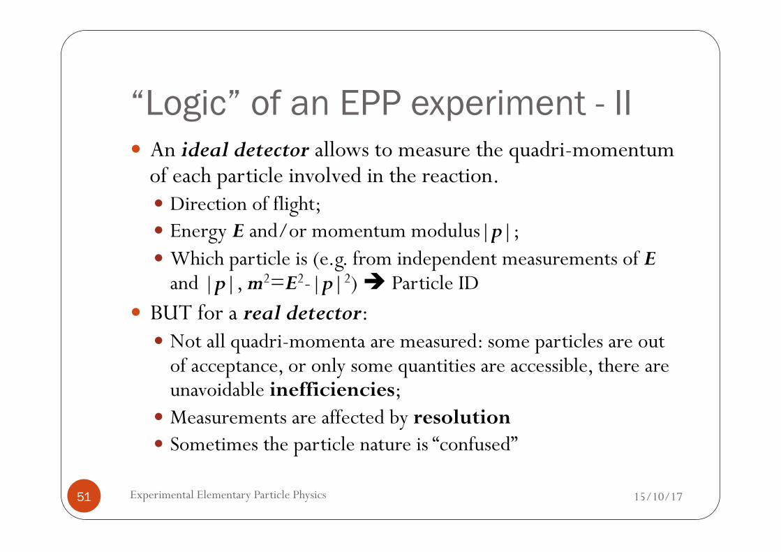
� An ideal detector allows to measure the quadri-momentum of each particle involved in the reaction. � Direction of flight; � Energy E and/or momentum modulus|p|; � Which particle is (e.g. from independent measurements of E
and |p|, m2=E2-|p|2) è Particle ID � BUT for a real detector:
� Not all quadri-momenta are measured: some particles are out of acceptance, or only some quantities are accessible, there are unavoidable inefficiencies;
� Measurements are affected by resolution � Sometimes the particle nature is “confused”
“Logic” of an EPP experiment - III
15/10/17 Experimental Elementary Particle Physics 52
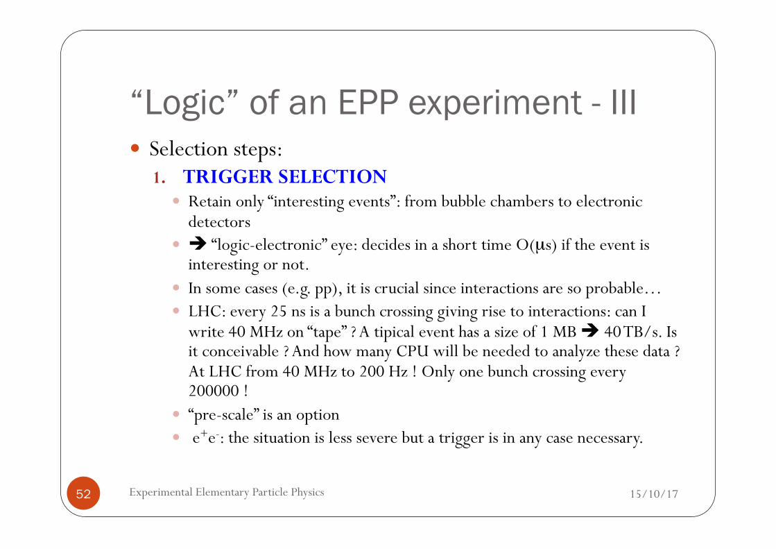
� Selection steps: 1. TRIGGER SELECTION
� Retain only “interesting events”: from bubble chambers to electronic detectors
� è “logic-electronic” eye: decides in a short time O(µs) if the event is interesting or not.
� In some cases (e.g. pp), it is crucial since interactions are so probable… � LHC: every 25 ns is a bunch crossing giving rise to interactions: can I
write 40 MHz on “tape” ? A tipical event has a size of 1 MB è 40 TB/s. Is it conceivable ? And how many CPU will be needed to analyze these data ? At LHC from 40 MHz to 200 Hz ! Only one bunch crossing every 200000 !
� “pre-scale” is an option � e+e-: the situation is less severe but a trigger is in any case necessary.
“Logic” of an EPP experiment - IV
15/10/17 Experimental Elementary Particle Physics 53
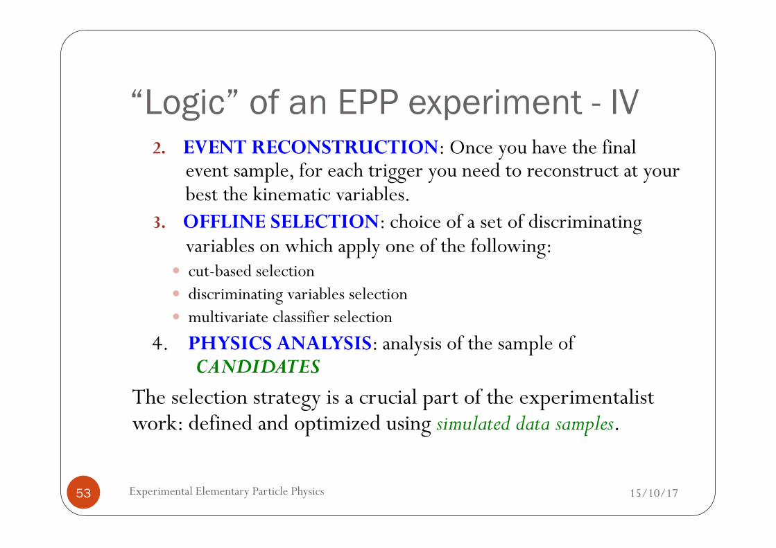
2. EVENT RECONSTRUCTION: Once you have the final event sample, for each trigger you need to reconstruct at your best the kinematic variables.
3. OFFLINE SELECTION: choice of a set of discriminating variables on which apply one of the following:
� cut-based selection � discriminating variables selection � multivariate classifier selection
4. PHYSICS ANALYSIS: analysis of the sample of CANDIDATES
The selection strategy is a crucial part of the experimentalist work: defined and optimized using simulated data samples.
“Logic” of an EPP experiment - V
15/10/17 Experimental Elementary Particle Physics 54
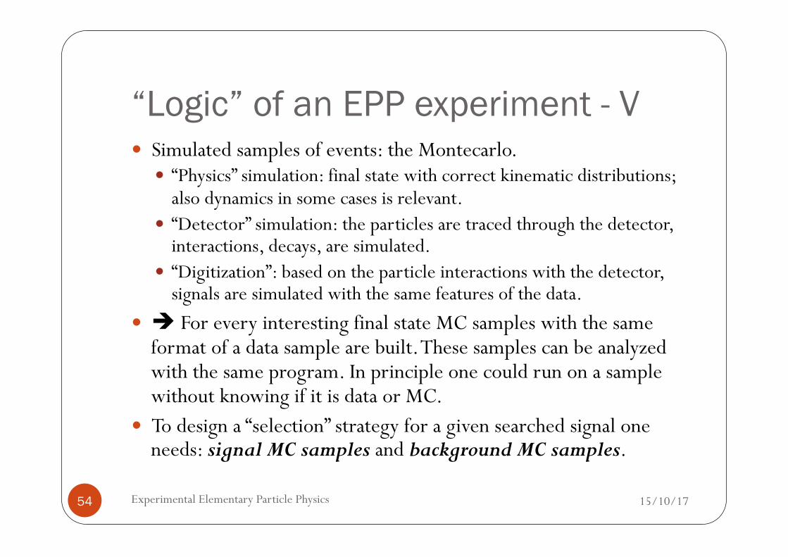
� Simulated samples of events: the Montecarlo. � “Physics” simulation: final state with correct kinematic distributions;
also dynamics in some cases is relevant. � “Detector” simulation: the particles are traced through the detector,
interactions, decays, are simulated. � “Digitization”: based on the particle interactions with the detector,
signals are simulated with the same features of the data. � è For every interesting final state MC samples with the same
format of a data sample are built. These samples can be analyzed with the same program. In principle one could run on a sample without knowing if it is data or MC.
� To design a “selection” strategy for a given searched signal one needs: signal MC samples and background MC samples.
“Logic” of an EPP experiment - VI
15/10/17 Experimental Elementary Particle Physics 55
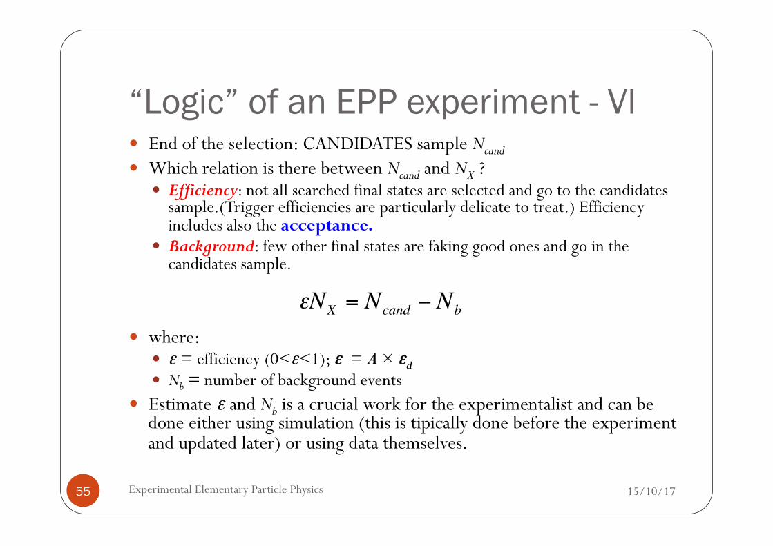
� End of the selection: CANDIDATES sample Ncand
� Which relation is there between Ncand and NX ? � Efficiency: not all searched final states are selected and go to the candidates
sample.(Trigger efficiencies are particularly delicate to treat.) Efficiency includes also the acceptance.
� Background: few other final states are faking good ones and go in the candidates sample.
� where: � ε = efficiency (0<ε<1); ε = A × εd � Nb = number of background events
� Estimate ε and Nb is a crucial work for the experimentalist and can be done either using simulation (this is tipically done before the experiment and updated later) or using data themselves.
€
εNX = Ncand − Nb
Quantities to measure
15/10/17 Experimental Elementary Particle Physics 56
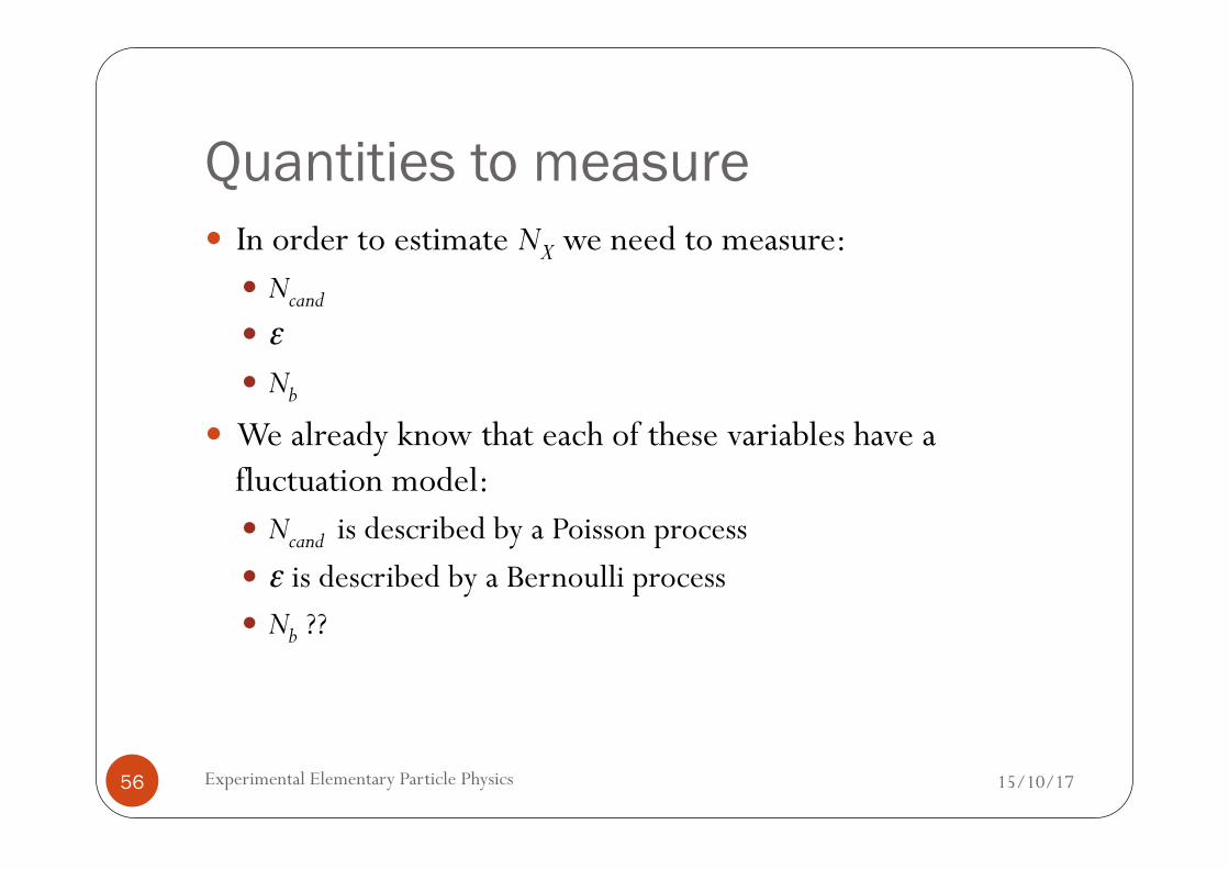
� In order to estimate NX we need to measure: � Ncand
� ε� Nb
� We already know that each of these variables have a fluctuation model: � Ncand is described by a Poisson process � ε is described by a Bernoulli process � Nb ??
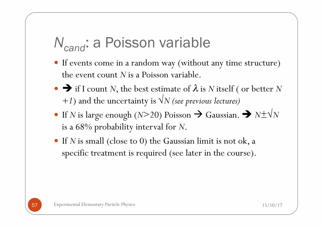
Ncand: a Poisson variable
15/10/17 Experimental Elementary Particle Physics 57
� If events come in a random way (without any time structure) the event count N is a Poisson variable.
� è if I count N, the best estimate of λ is N itself ( or better N+1) and the uncertainty is √N (see previous lectures)
� If N is large enough (N>20) Poisson à Gaussian. è N±√N is a 68% probability interval for N.
� If N is small (close to 0) the Gaussian limit is not ok, a specific treatment is required (see later in the course).
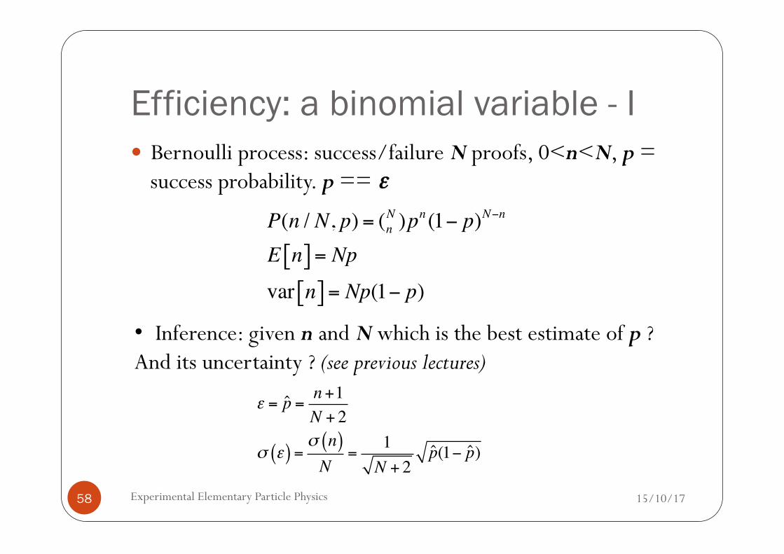
Efficiency: a binomial variable - I
15/10/17 Experimental Elementary Particle Physics 58
� Bernoulli process: success/failure N proofs, 0<n<N, p = success probability. p == ε
P(n / N, p) = (nN )pn (1− p)N−n
E n[ ] = Npvar n[ ] = Np(1− p)
• Inference: given n and N which is the best estimate of p ? And its uncertainty ? (see previous lectures)
ε = p̂ = n+1N + 2
σ ε( ) =σ n( )N
=1N + 2
p̂(1− p̂)
Efficiency: a binomial variable - II
15/10/17 Experimental Elementary Particle Physics 59
� How measure it ? � From data: Sample of N true particles and I measure how many,
out of these give rise to a signal in my detector � From MC: I generate Ngen “signal” events. If I select Nsel of these
events out of Ngen, the efficiency is (assume Ngen and Nsel large numbers):
ε =Nsel
Ngen
σ ε( ) =σ Nsel( )Ngen
=1Ngen
Nsel
Ngen
1− Nsel
Ngen
"
#$$
%
&''
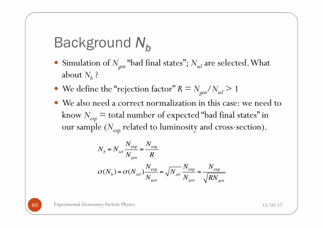
Background Nb
15/10/17 Experimental Elementary Particle Physics 60
� Simulation of Ngen “bad final states”; Nsel are selected. What about Nb ?
� We define the “rejection factor” R = Ngen/Nsel > 1 � We also need a correct normalization in this case: we need to
know Nexp = total number of expected “bad final states” in our sample (Nexp related to luminosity and cross-section).
Nb = NselNexp
Ngen
=Nexp
R
σ (Nb ) =σ (Nsel )Nexp
Ngen
= NselNexp
Ngen
=Nexp
RNgen
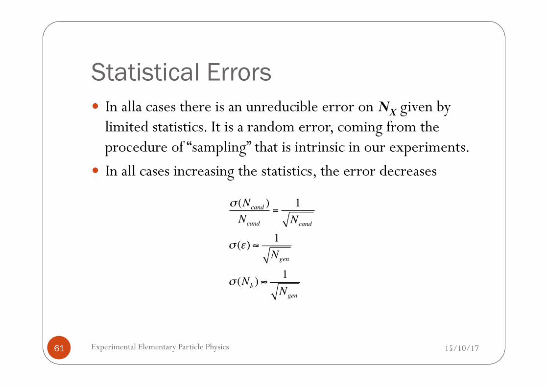
Statistical Errors
15/10/17 Experimental Elementary Particle Physics 61
� In alla cases there is an unreducible error on NX given by limited statistics. It is a random error, coming from the procedure of “sampling” that is intrinsic in our experiments.
� In all cases increasing the statistics, the error decreases
σ (Ncand )Ncand
=1Ncand
σ (ε) ≈ 1Ngen
σ (Nb ) ≈1Ngen
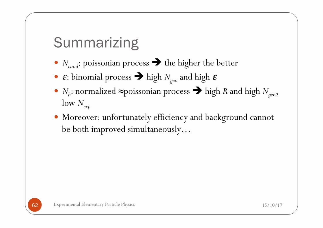
Summarizing
15/10/17 Experimental Elementary Particle Physics 62
� Ncand: poissonian process è the higher the better � ε: binomial process è high Ngen and high ε� Nb: normalized ≈poissonian process è high R and high Ngen,
low Nexp
� Moreover: unfortunately efficiency and background cannot be both improved simultaneously…
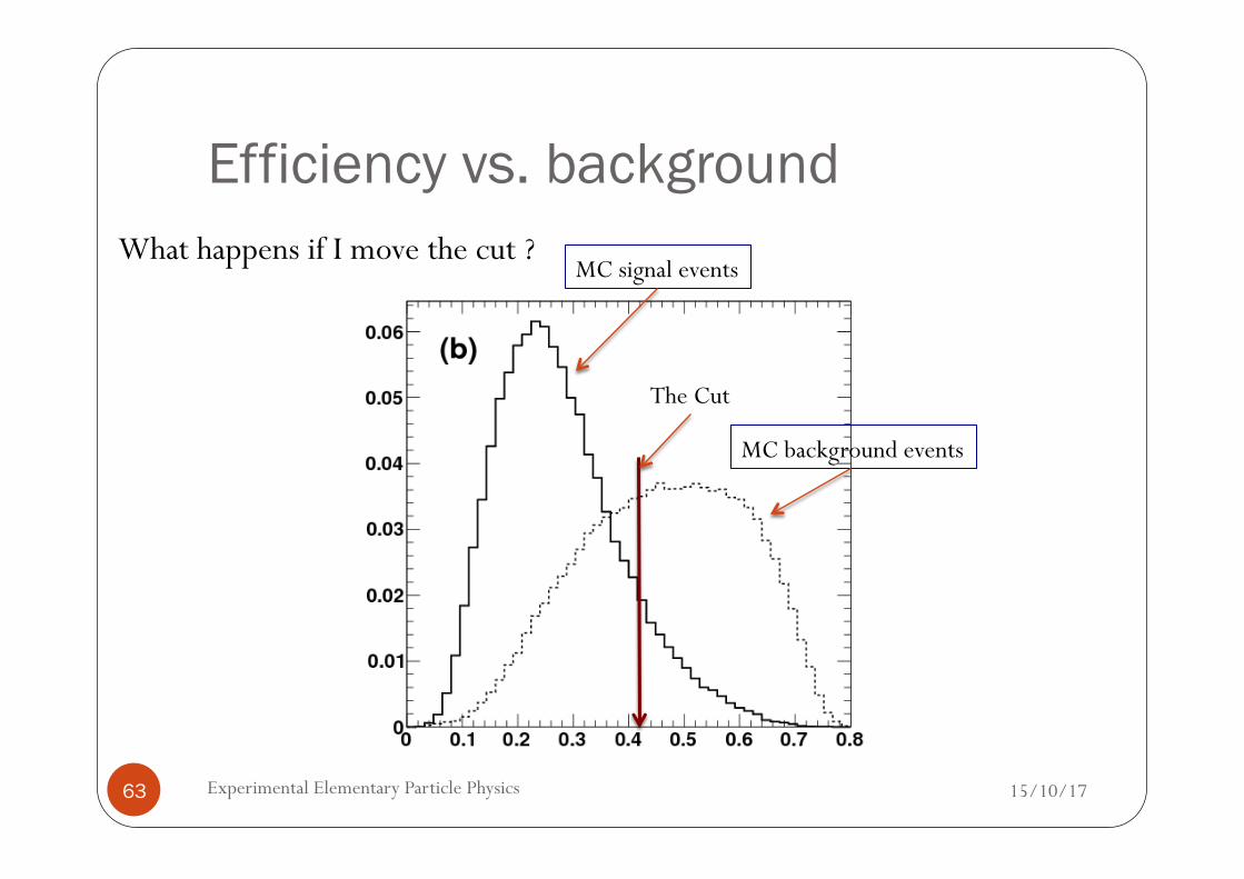
Efficiency vs. background
15/10/17 Experimental Elementary Particle Physics 63
MC signal events
MC background events
The Cut
What happens if I move the cut ?
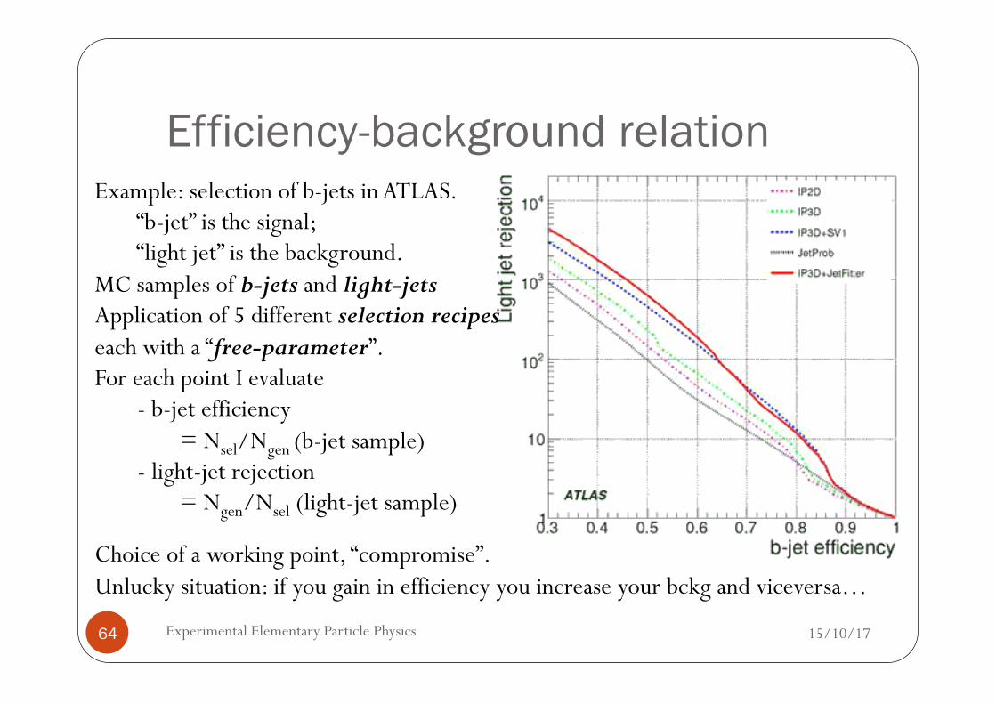
Efficiency-background relation
15/10/17 Experimental Elementary Particle Physics 64
Example: selection of b-jets in ATLAS. “b-jet” is the signal; “light jet” is the background.
MC samples of b-jets and light-jets Application of 5 different selection recipes each with a “free-parameter”. For each point I evaluate
- b-jet efficiency = Nsel/Ngen (b-jet sample) - light-jet rejection = Ngen/Nsel (light-jet sample)
Choice of a working point, “compromise”. Unlucky situation: if you gain in efficiency you increase your bckg and viceversa…
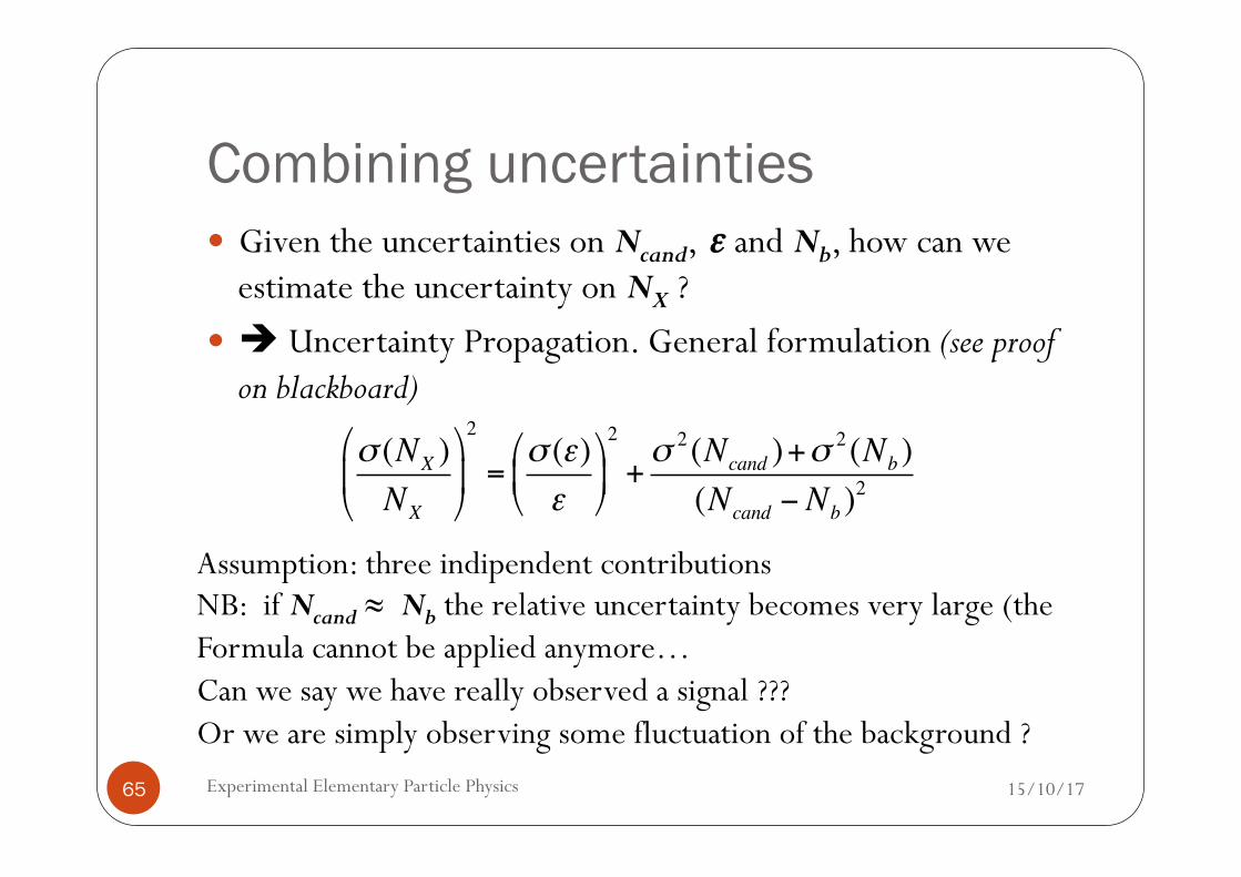
Combining uncertainties
15/10/17 Experimental Elementary Particle Physics 65
� Given the uncertainties on Ncand, ε and Nb, how can we estimate the uncertainty on NX ?
� è Uncertainty Propagation. General formulation (see proof on blackboard)
σ (NX )NX
!
"#
$
%&
2
=σ (ε)ε
!
"#
$
%&2
+σ 2 (Ncand )+σ
2 (Nb )(Ncand − Nb )
2
Assumption: three indipendent contributions NB: if Ncand ≈ Nb the relative uncertainty becomes very large (the Formula cannot be applied anymore… Can we say we have really observed a signal ??? Or we are simply observing some fluctuation of the background ?
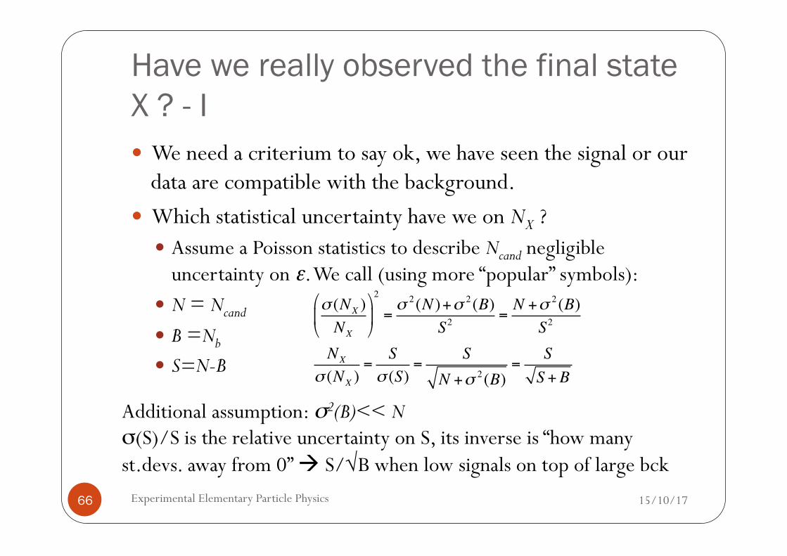
Have we really observed the final state X ? - I
15/10/17 Experimental Elementary Particle Physics 66
� We need a criterium to say ok, we have seen the signal or our data are compatible with the background.
� Which statistical uncertainty have we on NX ? � Assume a Poisson statistics to describe Ncand negligible
uncertainty on ε. We call (using more “popular” symbols):
� N = Ncand
� B =Nb � S=N-B
Additional assumption: σ2(B)<< N σ(S)/S is the relative uncertainty on S, its inverse is “how many st.devs. away from 0” à S/√B when low signals on top of large bck
σ (NX )NX
⎛
⎝⎜
⎞
⎠⎟
2
=σ 2 (N )+σ 2 (B)
S2=N +σ 2 (B)
S2
NX
σ (NX )=
Sσ (S)
=S
N +σ 2 (B)=
SS +B
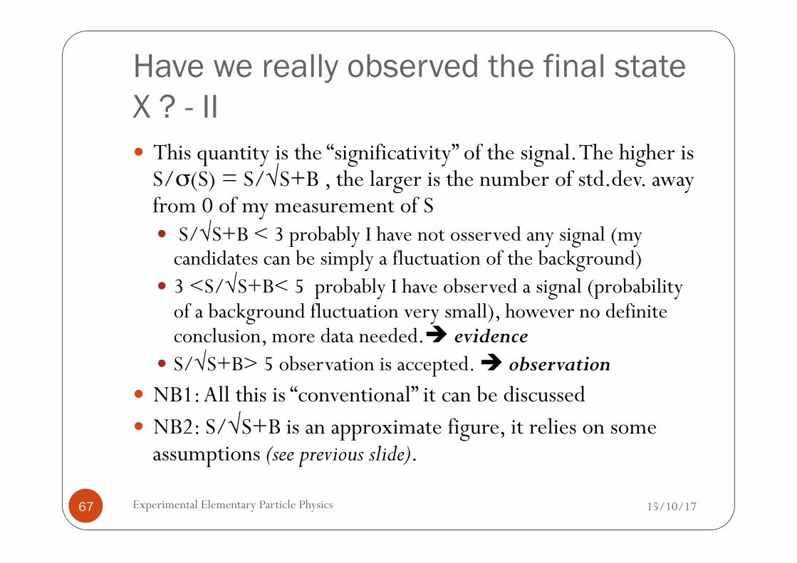
Have we really observed the final state X ? - II
15/10/17 Experimental Elementary Particle Physics 67
� This quantity is the “significativity” of the signal. The higher is S/σ(S) = S/√S+B , the larger is the number of std.dev. away from 0 of my measurement of S � S/√S+B < 3 probably I have not osserved any signal (my
candidates can be simply a fluctuation of the background) � 3 <S/√S+B< 5 probably I have observed a signal (probability
of a background fluctuation very small), however no definite conclusion, more data needed.è evidence
� S/√S+B> 5 observation is accepted. è observation � NB1: All this is “conventional” it can be discussed � NB2: S/√S+B is an approximate figure, it relies on some
assumptions (see previous slide).
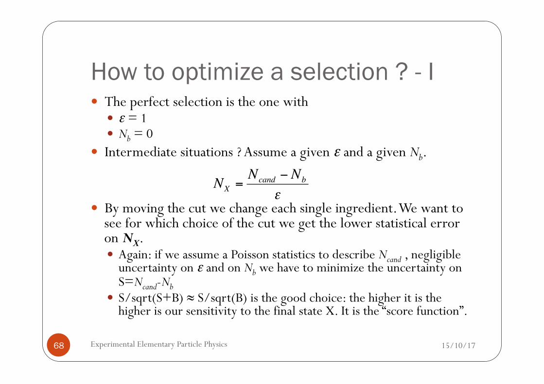
How to optimize a selection ? - I
15/10/17 Experimental Elementary Particle Physics 68
� The perfect selection is the one with � ε = 1 � Nb = 0
� Intermediate situations ? Assume a given ε and a given Nb. � By moving the cut we change each single ingredient. We want to
see for which choice of the cut we get the lower statistical error on NX. � Again: if we assume a Poisson statistics to describe Ncand , negligible
uncertainty on ε and on Nb we have to minimize the uncertainty on S=Ncand-Nb
� S/sqrt(S+B) ≈ S/sqrt(B) is the good choice: the higher it is the higher is our sensitivity to the final state X. It is the “score function”.
€
NX =Ncand − Nb
ε
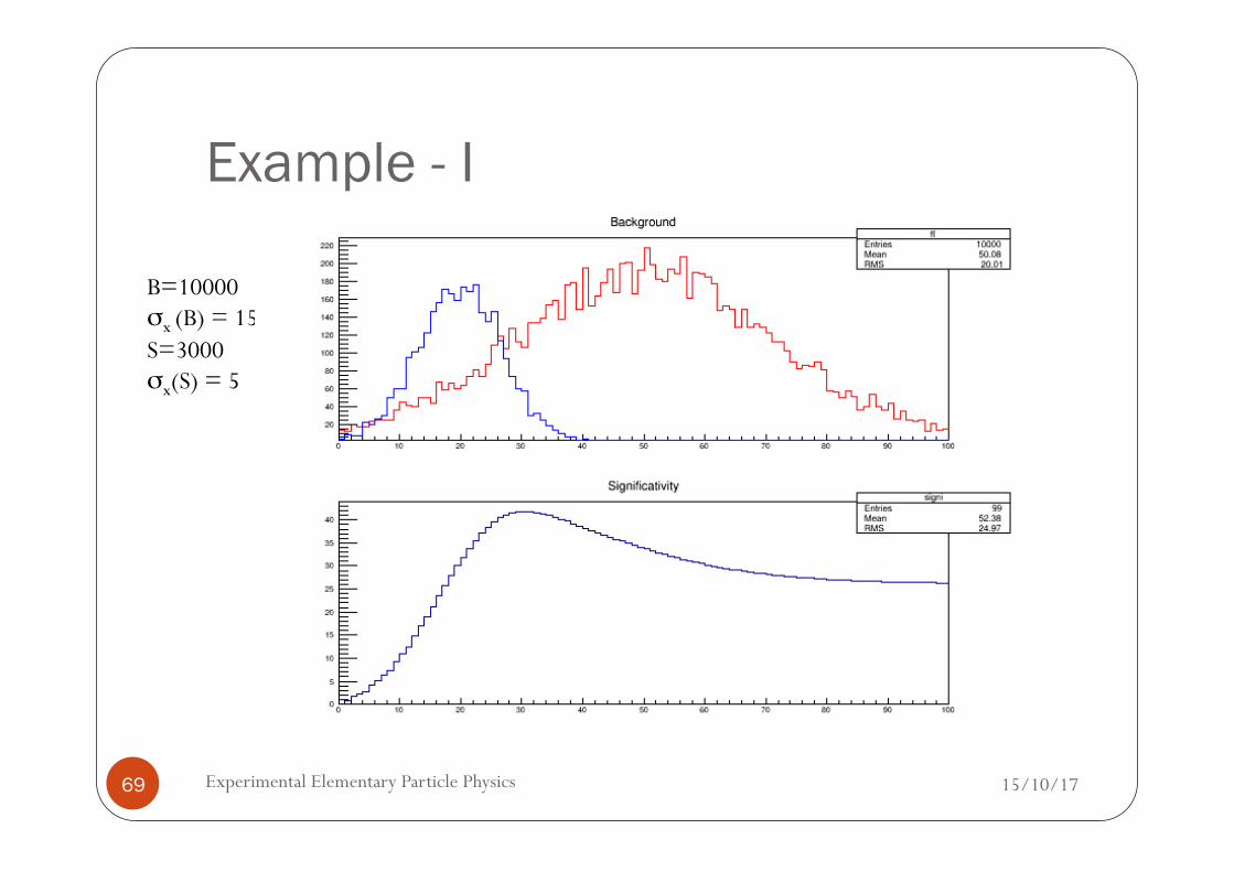
Example - I
15/10/17 Experimental Elementary Particle Physics 69
B=10000 σx (B) = 15 S=3000 σx(S) = 5
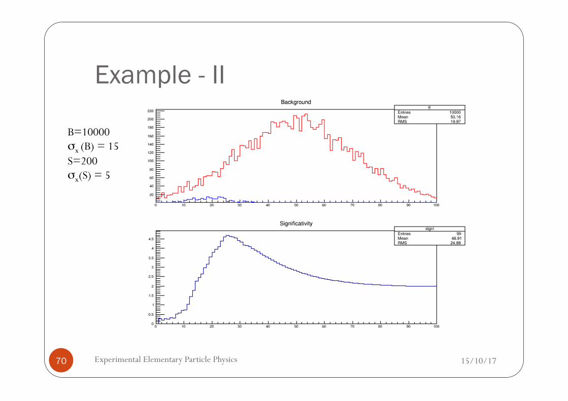
Example - II
15/10/17 Experimental Elementary Particle Physics 70
B=10000 σx (B) = 15 S=200 σx(S) = 5
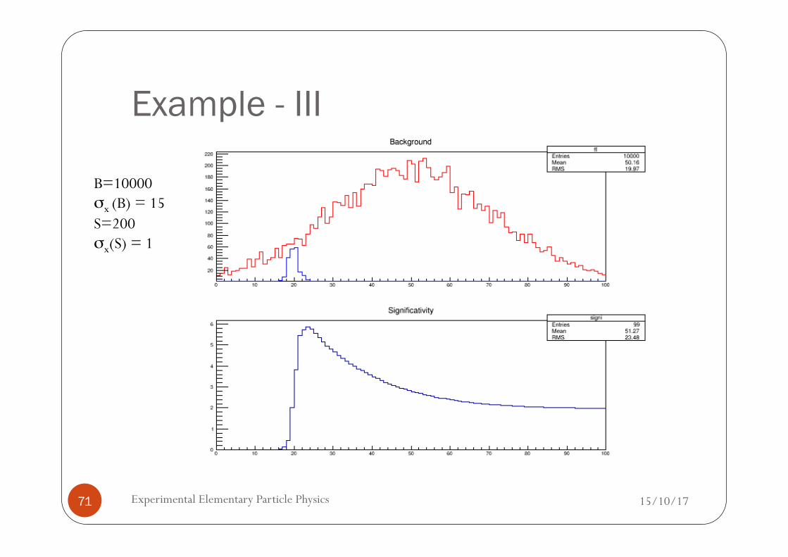
Example - III
15/10/17 Experimental Elementary Particle Physics 71
B=10000 σx (B) = 15 S=200 σx(S) = 1
Normalization
15/10/17 Experimental Elementary Particle Physics 72
� In order to get quantities that can be compared with theory, once we have found a given final state and estimated NX with its uncertainty we need to normalize to “how many collisions” took place.
� Measurement of: � Luminosity (in case of colliding beam experiments); � Number of decaying particles (in case I want to study a decay); � Projectile rate and target densities (in case of a fixed target
experiements). � Several techniques to do that, all introducing additional
uncertainties (discussed later in the course). � Absolute vs. Relative measurements.
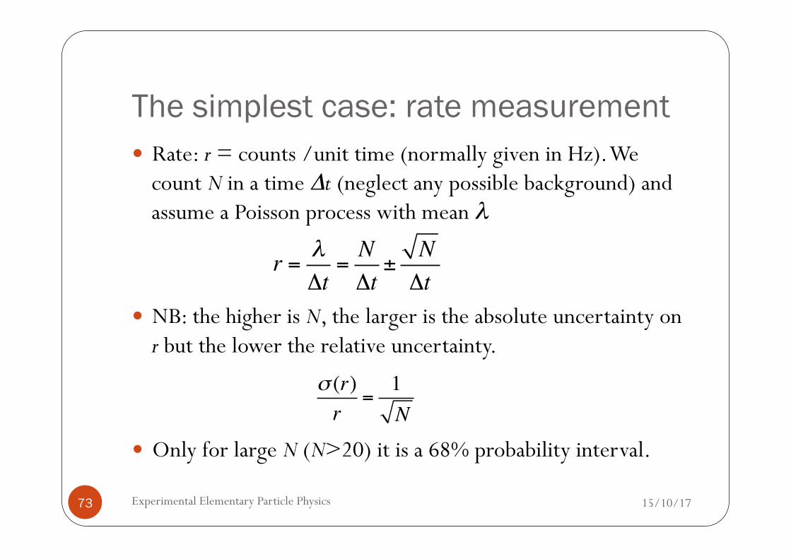
The simplest case: rate measurement
15/10/17 Experimental Elementary Particle Physics 73
� Rate: r = counts /unit time (normally given in Hz). We count N in a time Δt (neglect any possible background) and assume a Poisson process with mean λ
� NB: the higher is N, the larger is the absolute uncertainty on r but the lower the relative uncertainty.
� Only for large N (N>20) it is a 68% probability interval.
r = λΔt
=NΔt±
NΔt
σ (r)r
=1N
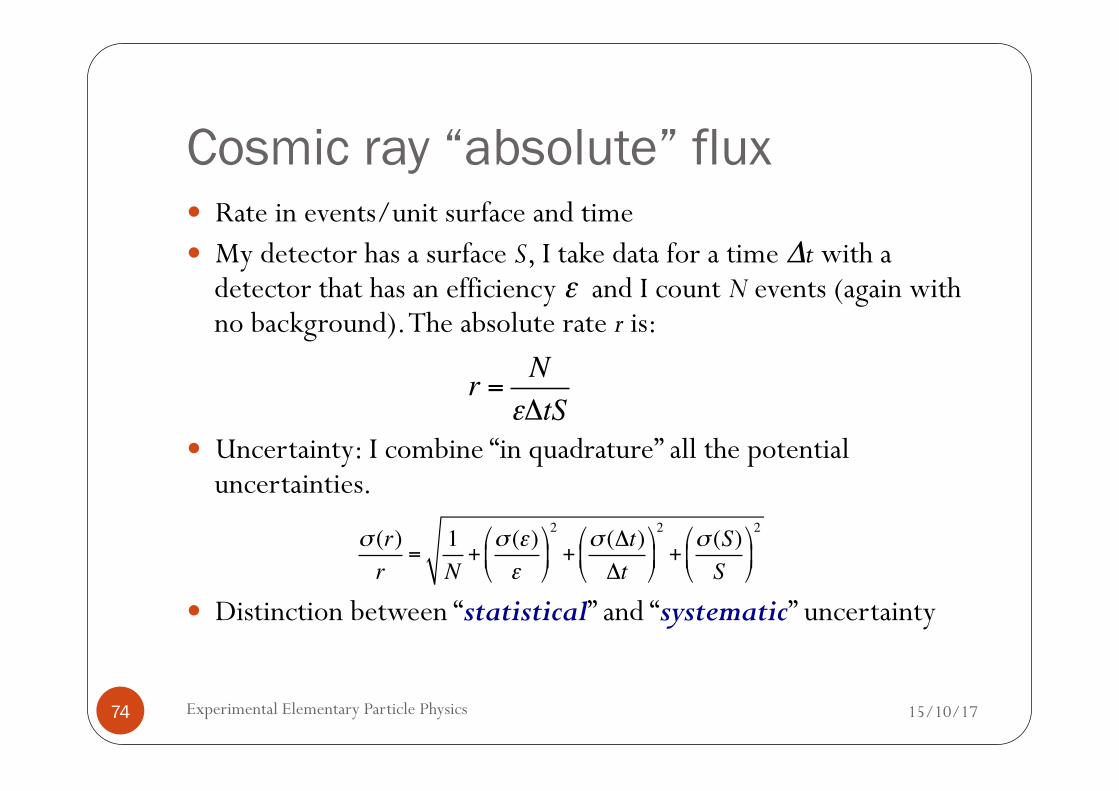
Cosmic ray “absolute” flux
15/10/17 Experimental Elementary Particle Physics 74
� Rate in events/unit surface and time � My detector has a surface S, I take data for a time Δt with a
detector that has an efficiency ε and I count N events (again with no background). The absolute rate r is:
� Uncertainty: I combine “in quadrature” all the potential uncertainties.
� Distinction between “statistical” and “systematic” uncertainty
r = NεΔtS
σ (r)r
=1N+σ (ε)ε
!
"#
$
%&2
+σ (Δt)Δt
!
"#
$
%&2
+σ (S)S
!
"#
$
%&2
Combination of uncertainties
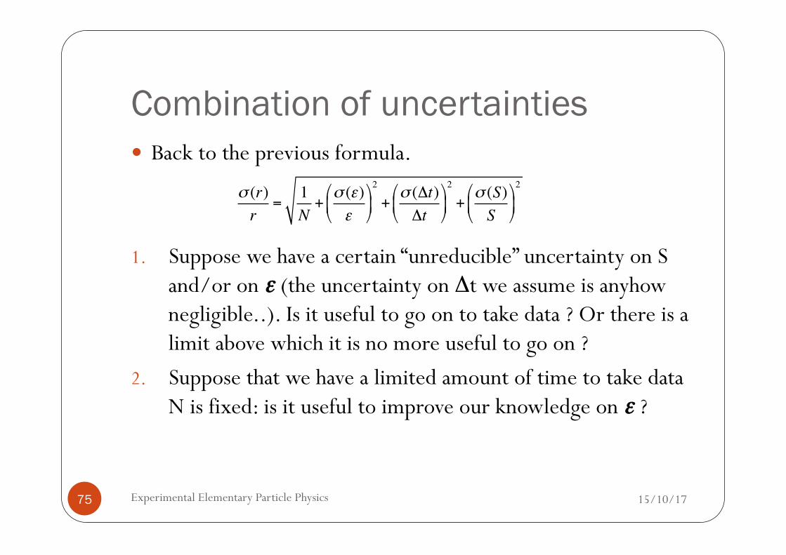
15/10/17 Experimental Elementary Particle Physics 75
� Back to the previous formula.
1. Suppose we have a certain “unreducible” uncertainty on S and/or on ε (the uncertainty on Δt we assume is anyhow negligible..). Is it useful to go on to take data ? Or there is a limit above which it is no more useful to go on ?
2. Suppose that we have a limited amount of time to take data N is fixed: is it useful to improve our knowledge on ε ?
σ (r)r
=1N+σ (ε)ε
!
"#
$
%&2
+σ (Δt)Δt
!
"#
$
%&2
+σ (S)S
!
"#
$
%&2
Not only event counting
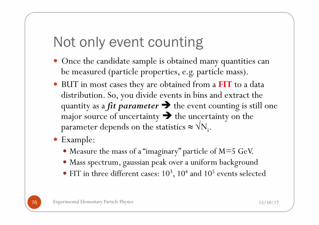
15/10/17 Experimental Elementary Particle Physics 76
� Once the candidate sample is obtained many quantities can be measured (particle properties, e.g. particle mass).
� BUT in most cases they are obtained from a FIT to a data distribution. So, you divide events in bins and extract the quantity as a fit parameter è the event counting is still one major source of uncertainty è the uncertainty on the parameter depends on the statistics ≈ √Ni.
� Example: � Measure the mass of a “imaginary” particle of M=5 GeV. � Mass spectrum, gaussian peak over a uniform background � FIT in three different cases: 103, 104 and 105 events selected
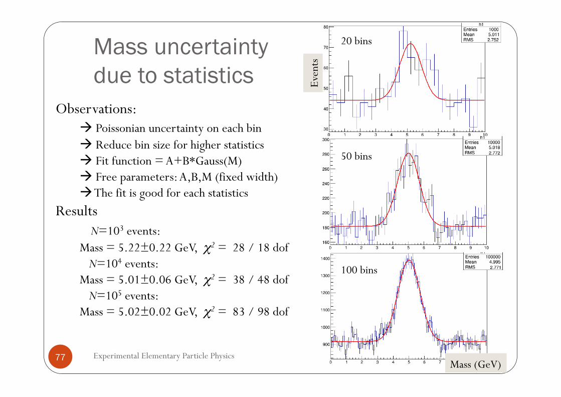
Mass uncertainty due to statistics
15/10/17 Experimental Elementary Particle Physics 77
Observations: à Poissonian uncertainty on each bin à Reduce bin size for higher statistics à Fit function = A+B*Gauss(M) à Free parameters: A,B,M (fixed width) à The fit is good for each statistics
Results N=103 events: Mass = 5.22±0.22 GeV, χ2 = 28 / 18 dof N=104 events: Mass = 5.01±0.06 GeV, χ2 = 38 / 48 dof N=105 events: Mass = 5.02±0.02 GeV, χ2 = 83 / 98 dof
Even
ts
Mass (GeV)
20 bins
50 bins
100 bins
Where could be a systematic uncertainty here ?
15/10/17 Experimental Elementary Particle Physics 78
� Absolute mass scale: this can be measured using a candle of known mass. Not always it is available. e.g. Z for the Higgs mass at the LHC.
� Mass resolution: in most cases the width of the peak is given by the experimental resolution that sometimes is not perfectly gaussian, giving rise to possible distortion to the curve.
� Physics effects: knowledge of the line-shape, interference with the background…
� In general: M = central value ± stat.uncert. ± syst.uncert.
Uncertainty combination
15/10/17 Experimental Elementary Particle Physics 79
central value ± stat.uncert. ± syst.uncert. Can we combine stat. and syst. ? If yes how ? The two uncertainties might have different probability meaning: typically one is a gaussian 68% C.L., the other is a “maximum” uncertainty, so in general it is better to hold them separate. If needed better to add in quadrature rather than linearly.
Summarizing
15/10/17 Experimental Elementary Particle Physics 80
� Steps of an EPP experiment (assuming the accelerator and the detector are there): � Design of a trigger � Definition of an offline selection � Event counting and normalization (including efficiency
and background evaluation) � Fit of “candidate” distributions
� Uncertainties � Statistical due to Poisson fluctuations of the event counting � Statistical due to binomial fluctuations in the efficiency
measurement � Systematic due to non perfect knowledge of detector effects.