ELSEVIER Journal of Applied Geophysics 41 (1999) 313-333

The location of infinite electrodes in pole-pole electrical surveys: consequences for 2D imaging

ouy a, Michel Dabas b, Marqbescloitres a, b, Pierre Mechler b, Alain $abbagh

IRD (ex-ORSTOM), 32 avenue H. Varagnat, 93143 Bondy Cedex, France UP&, U d R 7619, Boite 105, 4place Jussieu, 75252 Paris Cedex 05, France

Received 10 June 1998; accepted 4 March 1999

Abstract

In 2D-multielectrode electrical surveys using the pole-pole array, the distance to 'infinite electrodes' is actually finite. As a matter of fact, the available cable length generally imposes a poor approximation of theoretical location of these electrodes at infinity. This study shows that in most of the cases, the resulting apparent resistivity pseudosection is strongly distorted. Numerical simulation validated by field test also shows that a particular finite array provides results that are as close as possible to the ones of the ideal pole-pole array. This is achieved when two conditions that are weaker than an infinite location are fulfilled: (i) the 'infinite electrodes' are placed symmetrically on both sides of the in-line electrodes with a spread angle of 30" and (ii) the length of 'infinite lines' is at least 20 times the greatest distance between in-line electrodes. The electrical 2D image obtained with @is enhanced array is the least distorted one with respect to the pole-pole image. The apparent resistivities are generally underestimated, but this deviation is almost homogeneous. Though the shift cannot be determined a priori, the interpretation of such an image with direct or inverse software designed for pole-pole data provides '

an accurate interpretation of the ground geometry. O 1999 Elsevier Science B.V. All rights reserved.

Keywords: Electrical prospecting; Fole-pole array; Remote electrode effects; Numerical modelling

1. Introduction

ElecGcal resistivity methods are frequently used in studies focusing on the determination of overburden geometry (Griffiths and Barker, 1993; Lamotte et al., 1994; Cherry et al., 1996; Robain et al., 1996). Actually, these indirect methods efficiently complete discrete direct observations such as those obtained íi-om pits and hand drilling. The improvement of computer-controlled multichannel resistivimeters using multielectrode arrays has led to an important development of electrical imaging for these subsurface surveys (Griffiths and Turnbull, 1985; Griffiths et al., 1990; Barker, 1992). Tens of electrodes may be connected to such a resistivimeter. Apparent resistivity measurements are

* Corresponding author. Tel.: + 33-1-480-25636; Fax: +33-14847-3088; E-mail: robain@ird.fr

0926-9851/99/$ - see front matter O 1999 Elsevier Science B.V. All rights reserved. FIL S0926-9851(99)00010-5

. . _ _ .I' . .

r

3 14 H. Rahain et al. / Journal of Applied Geophysics 41 (1999) 313-333

recorded sequentially sweeping any quadripole-A B (current electrodes) M N (potential electrodes) -within the multielectrode array. As a result, high-definition pseudosections with dense sampling of apparent resistivity variation at shallow depth (0-100 m), are obtained in a short time. It allows detailed direct or inverse interpretation of 2D resistivity distribution in the ground (Shima, 1990; Loke and Barker, 1996).

The pole-pole array, noted ‘PP7, is frequently used. This array corresponds to a quadripole where electrodes B and N are placed ‘at infinity’ so that their influence may be ignored with respect to much closer electrodes A and M. Several reasons explain this choice.

(i) The investigation depth of this array is greater than any other (Roy and Apparao, 1971). Hence, deep targets are better detected than with any other configuration. On the contrary, it should be noted that this property also results in a lack of resolution at shallow depth.

(ii) This array provides weak edge effects; particularly symmetrical inhofnogeneities in the ground are imaged as symmetrical anomalies (Brunel, 1994). Hence, apparent resistivity pseudosections exhibit clear patterns which reliably guide the interpretation processes.

(iii) The large MN distance provides a higher signal for the pole-pole array compared to any other array. Hence, current intensity generally has not to be increased during the acquisition process. Nevertheless, the noise, which is proportional to t;he length of the dipole, also increases. Hence, the outcome of signal/noise ratio is difficult to predict.

(iv) The apparent resistivity corresponding to any other array may be derived from pole-pole data (Parasnis, 1997). This flexibility allows comparison to data acquired with any other array and the use of any interpretation software. Beard and Tripp (1995), however, pointed out that even a small amount of noise on PP data reduces the accuracy of such reconstruction.

In order to really benefit from the above advantages, it is important to “ i z e a possible cause of measurement noise linked to the array geometry. Actually, when PP is chosen, the problem is to move away B and N electrodes as far as possible in order to approach their theoretical location at infinity. Literature states that ‘infinite lines’ should be 10 to 20 times longer than AM distance (Keller and Frischknecht, 1966; Telford et al., 1990). Such an ‘infinite’ distance should also be respected between both ‘infinite’ electrodes B and N. Though it is generally not specified, for many field surveys using multielectrode PP, the length of ‘infinite lines’ does not reach more than 5 to 10 times the greatest AM distance. These finite-arrays, called pseudo-pole-pole arrays in this paper and further noted ‘psPP’, are considered equivalent to PP. However, the electrical image obtained using psPP may be different from the one corresponding to PP. Hence, the use of psPP data set with 2D modelling software designed for PP data could lead to misinterpretation.

This paper aims at quantifying these differences and at proposing some practical solutions to obtain with psPP a field data set as close as possible to the one which would have been obtained with PP.

2. Materials and methods

This section presents (i) the geometrical characteristics of different multielectrode psPP defined by changing the location of the ‘infinite’ electrodes, (ii) the usual field procedure for a survey using such arrays, (iii) the numerical simulation used to compute apparent resistivity deviation when using psPP instead of PP and (iv) the analytical calculation needed to define a psPP geometrically equivalent to PP. The test site used for field validation of numerical simulations is presented at the end of Section 3.

H. Rahain et al./ Janrnal afApplied Geaphysics 41 (1999) 313-333 315

2.1. nie multielectrode pseudo-pole-pole arrays (psPP)

We have simulated multielectrode psPPs with 23 electrodes (Fig. 1). These arrays are composed of 21 collinear eleceodes fixed with a regular inter-electrode spacing at positions noted E,. . . E2,. Electrodes A and M are chosen within this set and noted A i and Mj, according to their position. For example, M, corresponds to electrode M chosen at position E,. The two last electrodes correspond to B and N. Their locations are chosen along the circle of center O which is the middle of the two extreme positions E, and E2,. It should be noted that we have limited this study to psPP with the same distance ON and OB. This corresponds to a realistic layout of cables for surveys in the open field where topography does not control the positioning of ‘infinite’ electrodes.

These multielectrode arrays are defined in this paper using four geometrical parameters. The first two are referred to collinear electrodes positions and the last two to ‘infinite’ electrodes positions.

The first one is the inter-electrode spacing and is noted d. Its expression is:

d=EiEi+1 (m), (1) where EiEi+ is the distance between two successive positions Ei and Ei+ have used d = 1 m.

For the simulations, we

The second one is called ‘half-extent of in-line electrodes’ and is noted D. Its expression is:

where E,E,, is the distance between the two eqtreme positions E, and E,. The third one is called ‘infinite length coefficient’ and is noted Q. Its expression is:

ON OB D D Q = - = - (dimensionless), (3)

where ON and OB are the distances between point O and electrodes N and B, respectively, and D is the ‘half-extent of in-line electrodes’ defined in the expression (2). The coefficient Q varies from 1 to 1000 in the simulations.

*y Fig. 1. Geometrical characteristics of the multielectrode pseudo-pole-pole array used. Solid circles: electrode positions.

316 H. Rohain et al./ Journal of Applied Geophysics 41 (1999) 313-333

' The two parameters called 'infinite line angles' and noted ß and Y are grouped in a single parameter called 'spread of infinite lines' and noted 0. Their expressions are, respectively:

ß = BÔE,, (")

Y = NÔE, (") (4)

(5) o= NÔB = Y- p (01, (6)

where BÔE,, is the angle between lines OB and OE2,, NÔE, is the angle between lines ON and OE,, and NOB is the angle between lines ON and OB. The spread 0 varies from O" to 180" in the simulations.

2.2. Usual field procedure for multielectrode pseudo-pole-pole surueys

By fixing electrode A, at position E, and switching sequentially electrodes Mj from positions E, to E20, the multielectrode psPP provides an electrical sounding with 20 measurement points (Fig. 2). The measurement points are conventionally located at the middle of electrodes A, and Mj and at a pseudodepth corresponding to half the distance between A, and Mj (Hallof, 1957). This results in a 45" inclined line. An apparent resistivity pseudosection, called '2D electrical image', may be considered as a collection of such soundings acquired with a step corresponding to spacing d. For practical reasons in field survey, measurements are generally taken for a l l combinations of two electrodes within the set of in-line electrodes. For y1 in-line electrodes, this results in a triangular image with n(n - 1)/2 measurement points. Overlapping between such triangles on the final 2D electrical image depends on the shift between one in-line array and the next.

2.3. Numerical simulation

The general moment method (Harrington, 1961) applied to electromagnetic 3D modelling (Tab- bagh, 1985) is used to compute the potential values at Mj and N locations due to a unit current flowing into the ground through electrodes A i (+) and B (-). This method was restricted in this simulation to contrast in electrical resistivity only. The accuracy of this numerical code for forward modelling was checked against published results obtained through algorithms that use either equiva- lent surface charge densities or finite-difference approach (Dabas et al., 1994). We have simulated measurements upon a ground made of three horizontal layers computing potential values for both PP and psPP. We empirically considered that the array was in PP configuration when potential values at electrodes Mj did not numerically depend on position of electrodes B and N.

Fig. 2. Electrical sounding obtained with pole-pole multielectrode array. Open triangle: A position, solid triangle: B successive positions, solid circles: conventional locations of apparent resistivity measurements.

H. Robain et al./ Journal of Applied Geophysics 41 (2999) 313-333 3 17

The apparent resistivity paiJ corresponding to measurement made with a quadripole AiBMjN is defined as:

where electrodes Mj and N (V) and I the current intensity (A).

as:

is the geometric coefficient of the quadripole (m), the potential difference between

The normalized difference between psPP and PP apparent resistivities, noted 6( pai,j), is defined

where pai,j and From definition (7), it yet appears that this difference between the apparent resistivities can be

caused by using an approximate expression for the geometrical factor and by the fact that the voltage measured from the finite electrode configuration is not identical to the ideal pole-pole configuration. Both effects will be analyzed here, beginning with the geometrical effect.

2.4. Calculation of geometrical coefStcìent

are the apparent resistivities corresponding to psPP and PP, respectively.

The geometrical coefficient of any A,BMjN quadripole, noted Kl , j , is defined as:

t- AiMj BMj A,N BN

where AiMi, BMj, A,N and BN are the distances between electrode pairs.

following expression which defines the PP geometrical coefficient, noted I?,,.: For PP, expressions l/BMj, l /A,N and 1/BN are nil. Hence, Eq. (9) may be simplified to the

= 27.rAiMj (m). (10) It should be noted that this simpMied coefficient (10) may be unsuitable for psPP which poorly

approximate the ideal location of electrodes B and N at infinity. In these cases, the general coefficient (9) must be used to calculate properly the apparent resistivity (Kunetz, 1966). This is particularly important because one of the prevalent commercial codes used for the interpretation of 2D electrical image only take into account ideal pole-pole configuration (RESIX2DI from INTERPEX). Hence, it is the simplified coefficient which is used to calculate the apparent resistivities when the inputs are the measured potentials. As this code also allows to directly input the apparent resistivities, it is preferable to prior calculate the accurate values. This precaution is nevertheless not satisfying because it is the ideal pole-pole coefficient which is used after words for inverse modelling. The most recent version of another leading commercial code (RES2DINV version 3.33 from LOKE, ABEM) allows to take into account the exact geometrical coefficient of psPP. It is clear that the owners of this code should ask for the upgraded version and use this new option.

The error made when using PP geometrical coefficient instead of psPP geometrical coefficient may be quantified by the normalized difference between the two coefficients. For the largest quadripole A,BM,,N, it is noted S( and is calculated as:

318 H. Rohain et aL/ Joartial of Applied Geophysics 41 (1999) 313-333

'I

4

2.D = n.d Fig. 3. Geometrical characteristics of any quadripole AiBMiN taken within the multielectrode array respect to A,BM,,N quadripole. Solid circles: electrode positions, open circles: center points.

The analytical development of Eq. (ll), detailed in Appendix A, gives the following third order approximation:

with

(12a)

This led us to limit the study to symmetrical arrays with opposite infinite line angles, for which expression (12b) simplifies as (the second order term is canceled for any parameter Q):

The coefficient for any other quadripole AiBMjN (Fig. 3), analogous to geometrical parameters introduced for the quadripole A,BM2,N in expressions (3) and (6), respec- tively, are defined as:

and the spread

Oi,jB Oi,jN Qi,j = - - -- (dimensionless) ,

Di, j Di,j

H. Rohain et al. / Journal of Applied Geophysics 41 (1999) 313-333 3 19

where Di,, is the half-distance between electrodes Ai and Mi; Oi,, is the middle of electrodes Ai and Mj; O,,B and O,N are the distances between point Oc, and electrodes B and Ny respectively.

= NÔ~,,B ("1 , (15) where NÔ,,,B is the angle between lines Oi,,N and Oi,jB.

in Eq. (13), allows to calculate the difference S ( K , , ) , for any quadripole AiBMjN within a symmetrical multielectrode psPP. Analytical derivations of coefficient Qi,j and spread Oi,, are given in Appendix B.

Hence, replacing coefficient Q with coefficient Qi,i and spread I9 with spread

3. Results and discussion

3. I . Pseudo-pole-pole array geonzetrìcally equivalent to pole-pole array

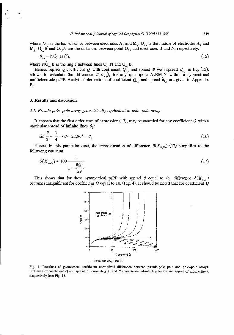
It appears that the first order term of expression (13), may be canceled for any coefficient Q with a particular spread of infinite lines 8,:

0 1 - sin - = -

2 4 I9= 28,96" = 19,.

Hence, in this particular case, the approximation of difference S(K,,,) (12) simplifies to the following equation.

1

8Q3 1--

29

(17) 6(K0,20) = 100

This shows that for these symmetrical psPP with spread I9 equal to O,, difference S(K,,.,,) becomes insignificant for coefficient Q equal to 10. (Fig. 4). It should be noted that for coefficient Q

180

150

120

60

30

O 1 10 100 1000

Coefficient Q

- ¡so-deviation 6(K,,m) lines (%)

Fig. 4. Isovalues of geometrical coefficient normalized difference between pseudo-pole-pole and pole-pole mays. Influence of Coefficient Q and spread 8. Parameters Q and 8 characterize infinite line length and spread of infinite lines, respectively (see Fig. 1).

r

320 H. Rohain et al./ Journal of Applied Ge0phy.sic.T 41 (1999,) 313-333

larger than 10, the first order term of approximation (12) is the predominant one even if the symmetry condition is not respected. This means that the spread of infinite lines is the only important parameter to achieve a psPP geometrically equivalent to PP. Hence, since the two conditions are respected (spread 6 equal to So and coefficient Q at least equal to lo), B and N may be moved around O without significant influence.

For small coefficient Q, the spread O, is not suitable to cancel the difference S(K,,,,). The suitable spread value tends towards zero as coefficient Q tends towards 1. This shows that even when 'infinite' lines are very small, there exists a symmetrical psPP geometrically equivalent to PP. But in these cases, a very weak variation of spread O results in a very large variation of difference 6( Hence, 'infinite lines' with small coefficient Q are not suitable in practice, even if geometrical equivalence between psPP and PP theoretically exists.

From a practical point of view, a difference 6( less than 2% in absolute value, similar to usual instrumental errors, is acceptable. Fig. 4 points out that the difference 6( is less than 2% for spreads O larger than 15" and coefficients Q larger than 150. However, such a large coefficient Q is not realistic (it corresponds to MN distance equal to 1 km for AM distance equal to 13.3 m). Consequently, a spread O close to spread O, is the most reliable one to keep satisfactory in any cases the geometrical equivalence between psPP and PP.

Distance along profile (m)

O 10 20 30 40 50 60 70 80 90 100 O i " ' " " " ' ' " " " " " " " " " " " " " " ' " " ~ " " C

-5

-10

h

v E s Q $ -5 -0 3 a, d

-1 o

-5

-1 o

Q = 10

F(K) %

2 1 O -1 -2 -3

-6

-1 o -1 8 -32

-56 -100

Q = 20

Q=40

Fig. 5. Geometrical coefficient normalized difference between pole-pole and pseudo-pole-pole surveys. Pseudo-pole-pole arrays with different coefficients Q are used to survey a 100-m profile without moving infinite electrodes. The spread 0 referred to the leftmost triangle is 30".

H. Rohain et al./ Journal of Applied Geophysics 41 (1999) 313-333 321

Finally, it appears that coefficient Q not smaller than 10 and spread 8 close to 30" are necessary conditions to practically obtain geometrical equivalence between symmetrical psPP and PP for A,M,. Such an array will be further referred as 'enhanced psPP'.

These conditions are valid for A,M,, the largest A,M,.. Too frequent shifts of 'infinite' electrodes in order to respect the geometrical equivalence are not compatible with efficient field survey. Hence, for the same position of infinite electrodes, the influence of other A,Mj position upon difference S( Ki , j ) is now examined. Fig. 5 shows the evolution of difference 6( Ki , j ) for simulated psPP surveys along a 100-m long profile with fixed 'infinite' electrodes. In all the cases, the difference S(Ki , j ) remains less than 2% for the first triangle. But for coefficient Q equal to 10, the difference exceeds 2% for most of the next triangle (Fig. Sa). For coefficient Q equal to 20, the reliable zone covers three triangles (Fig. 5b). In fact, coefficient Q equal to 40 is necessary to keep geometrical equivalence satisfactory for the whole profile (Fig. 5c). It should be remembered that the use of a spread 8 different from 30" gives worse results in all cases.

It can already be noted that for a homogeneous ground, the error made upon apparent resistivity using the simplified coefficient I?j,j instead of exact coefficient Ki,j: will lead to an erroneous 2D electrical image, proportional to the sections presented in Fig. 5. It is clear that an image like the topmost one will not be interpreted as a homogeneous ground, but as a ground with a major lateral trend. In fact, for this simple case, the pattern of erroneous 2D electrical image only reflects the changes of the psPP geometrical parameters.

3.2. Apparent resistivity deviation with enhanced pseudo-pole-pole array

The problem is now to examine if geometrical equivalence is a sufficient condition to obtain the same apparent resistivity values with PP and enhanced psPP. This property is further called in this paper 'electrical equivalence'. This is not obvious because B and N are not at infinity and thus influence the potential difference AV used in Eq. (4) to calculate the apparent resistivity pa. Hence, even if the difference between geometrical coefficients S ( K ) is small, the difference between apparent resistivities S( pa) may be high if the difference between potential differences 6(AV) is.

3.3. Sensitivity to the array geometry

The sensitivity to array geometry is examined using the same ground model for the simulations of different psPP measurements. Resistivities and thickness of the three layers are, from top to bottom: 100 a m , 1000 O m and 10000 a m and 0.5 m, 5 m, infinite, respectively (model 1). Apparent resistivities are always calculated using the exact expression (9) of geometrical coefficient Ki,,.. The difference S( pa,,,) is computed for different coefficients Q and spread 19 varying in 0-180" range (Fig. 6a). All the curves have a similar shape. Smallest spreads 8 correspond to an extreme underestimation (positive difference). The difference S( paoqo) then decreases quickly with spread 8, the larger coefficient Q, the smaller spread 6 for which " n u m difference S( is reached. It should be noted that for large coefficient Q, this mínimum corresponds to a severe overestimation (negative difference). At last, difference 6( pa,,2,) tends asymptotically towards a local maximum reached for spread 8 equal to 180". This last point always correspond to an underestimation. For coefficient Q equal to 10, It appears that the least difference corresponds to a severe underestimation (17%). Contrary to the difference S( whose canceling is possible with any coefficient Q (Fig. 6b), canceling of the difference S( pa,,,) requires coefficient Q higher than 40. Section 2 concluded that coefficient Q larger than 10 was necessary to practically achieve geometrical equivalence. It

322 H. Rohain et al./ Journal of Applied Geophysics 41 (1999) 313-333

a- b-

U - 2 0 , . . I ) I , . . , . . I I , . ,

O 30 60 90 120 150 180

e

-30 4

O 30 60 90 120 150 180

0

Fig. 6. Apparent resistivity and geometrical coefficient normalized differences between pole-pole and pseudo-pole-pole arrays. Influence of coefficient Q and spread O. Cross hatched zone corresponds to difference less than 2% in absolute value.

appears here that coefficient Q larger than 40 is necessary to also achieve electrical equivalence. For these large coefficients Q, there are two intervals of spread 8 giving a difference S( pa,,,) smaller than 2% in absolute value. (i) A narrow interval at small spread range: the larger coefficient Q, the narrower this first interval. (ii) A large inteyal including spread 8,: the larger coefficient Q, the larger this second interval. It should be noted that in this second interval, the spread which gives electrical equivalence tends towards the spread 8, which gives geometrical equivalence as coefficient Q becomes larger.

Fig. 7 explains how electrical equivalence may be obtained with enhanced psPP. Fig. 7a shows the potential field generated by PP at the ground surface, In the case of a homogeneous ground, isopotentials correspond to concentric circles. The zero potential line is at infinity. Fig. 7b shows the potential field generated by enhanced psPP. The potential field is different from the previous one. It has a positive part at electrode A side and a negative part at electrode B side. Isopotential lines consist in two series of hyperbolas whose focuses are electrodes A and B, respectively. The two parts are separated by a zero potential straight line perpendicularly crossing the middle of line AB. It is clear that potentials measured at electrode M with both PP and psPP are different. This difference increases with AM distance. For the enhanced psPP giving electrical equivalence, the change of positive potential measured at electrode M is complemented by the negative potential measured at electrode N. Hence, though the potential fields are different, PP and enhanced psPP give close potential differences AV. Finally, as a consequence of geometrical equivalence, the apparent resistivities calculated with Eq. (7) for enhanced psPP and PP are close.

Like in Section 2, the influence of electrodes Ai and Mj positions upon differences S( pai,j) is now examined for the same position of infinite electrodes. The 20 differences S( of a psPP

H. Rohain et al./Joihmal of Applied Geophysics 41 (1999) 313-333

Potential field of pole-pole array (B and N at infinity)

Potential field of enhanced pseudo pole-pole array

323

-50 O 50 -50 O 50

Fig. 7. Potential field generated by pole-pole and pseudo-pole-pole arrays upon a homogeneous ground. Injected current is 1 A and ground resistivity is 628 Qm. Electrical equivalence with pole-pole array is obtained by using enhanced pseudo-pole-pole array.

electrical sounding are computed for different coefficient Q and spread 8 varying in 0-180" range (Fig. S). It appears that the difference S( paoj) may vary a lot with distance A,M,. In these cases, the

Q = 2 0 Q=40 40

20

h g h p 10

x .- z o 5

Q

K I-

U

-1 o

-20

-30 L

15

10

5

O

-5

-10

-1 5

-20 j / 3""

-25 L

Q = 8 0

lo I

-10 -

-15 -

-20 -

-25 1- O 5 10 15 20 O 5 10 15 20 O 5 10 15 20

distance AoMj (m) distance %Ml (m) distance AoMl (,,,I

Fig. 8. Apparent resistivity normalized differences between pole-pole and pseudo-pole-pole soundings. Influence of coefficient Q and spread 8 upon differences corresponding to each distance A,Mj. Cross hatched zone corresponds to difference less than 2% in absolute value.

324 H. Rohain et al./ Journal of Applied Geophysics 41 (1999) 313-333

sounding curves are severely distorted by an underestimation of apparent resistivity values rapidly increasing with distance A,M,. For the same spread 8, the smaller the coefficient Q, the more pronounced is this distortion. For the same coefficient Q, small spreads 8 give the highest distortions. Large spreads 8 are also unfavorable. In a l l cases, the least distortion is obtained with the spread 8, because differences S( pa,,,) are more homogeneous than with any other spread. Hence, the use of spread 8, will principally shift the sounding curve along apparent resistivity axes without major distortions.

Apparent resistivity deviations for this ground model are also simulated along a 100-m profile (Fig. 9). Coefficient Q equal to 20 is not sufficient to obtain weak distortion for the first triangle. For coefficient Q equal to 40, it appears that reliable values may be obtained only for the first three triangles (see Fig. 5 for comparison). For further triangles, though geometrical equivalence is satisfactory, a lateral distortion appears erroneously suggesting 2D structure. It should be remembered that any other psPP will give even worse results.

3.4. Sensitivity to the ground model

The sensitivity to the ground model is examined using another ground model with layers of same thickness, but different resistivities (Fig. 10). Resistivities of the three layers are 1000 a m , 100 a m and 10000 R m from top to bottom (model 2). It appears that for the same psPP, difference S( pa,,,) may vary a lot depending on ground property. Partiçularly for the spread e,, the mean difference 6( paoj) is negligible for model 1, but corresponds to a severe underestimation for model 2. This shows that a correction of psPP data cannot be practically achieved because the ground model is needed to estimate the difference 6( pa). Nevertheless, for both models, the spread corresponds to

n i ' ' ' t Q=20

E 5 Y

% -5

z U O

U 3 a,

-1 o O

-5

-1 o

Q=40

S(pa) %

15.8 12.6 10.0 7.9 6.3 5.0 4.0 3.2 2.5 2.0

1.6 1.3 1 .o 0.0

O 10 20 30 40 50 60 70 80 90 100

Distance along profile (m)

Fig. 9. Apparent resistivity normalized difference between pole-pole and a pseudo-pole-pole surveys. Pseudo-pole-pole arrays with different coefficients Q are used to survey a 100-m profile without moving infinite electrodes. The spread 8 referred to the leftmost triangle is 30".

I . ,

'

H. Rohain et al./ Journal ofApplied Geophysics 41 (1999) 313-333 325

2o $1 Modell

c

s = -20i Q=40

-301 - a I I I I 1 I I I I I I I I I I O 30 60 90 120 150 180

T 1 Model 2 h

E 40 5- B O

a, "I 30 s I e

x 20 m

Q

c 10 s l00Q.m

IM:PI IOOOQ.~

0 IOOOO Q.m

Angle 8

Fig. 10. Apparent resistivity normalized difference between pole-pole and a pseudo-pole-pole soundings upon two different ground models. Influence of spread 0 upon mean and dispersion values. Cross hatched zone corresponds to differences of less than 2% in absolute value.

the least standard deviation. Hence, in both cases, the pattern of the sounding curve obtained with enhanced psPP is the least distorted one.

The influence of the ground model is tested more exhaustively for the enhanced psPP (Fig. 11). Fig. l l a shows that increasing the resistivity of the intermediate layer in model 1 has no significant influence upon the differences 6( On the contrary, decreasing the resistivity of this layer results in an important rise of both mean and standard deviation values of differences a( paQj). Fig. l l b shows that reducing the thickness of the topmost resistive layer in model 2 results in a more distorted sounding curve. The mean value of differences S( paoJ) remains the same, but the standard deviation becomes higher. On the contrary, the mean value of differences 6( decreases when increasing the thickness of this layer. The standard deviation increases at first, but collapses as the influence of the underlying conductive layer disappears. It can be concluded that sounding curves have great distortions when a conductive layer preeminently influences the apparent resistivities, whether with large thickness or with low resistivity.

326

h E

O (v a, 5 L

P - m Q

40

30

20

10

O

H. Robain et ai./ Journal of Applied Geophysics 41 (1999) 313-333

a-

T Q=40 Model X,

O

0 P2

5 a

20 1 I 0 ModelX2 El a

5

0.1 1 10 1 O0 1 O00

Thickness of first layer (m)

Fig. 11. Apparent resistivity normalized difference between pole-pole and an enhanced pseudo-pole-pole soundings. Influence of layers' thickness and resistivities upon mean and dispersion values. Cross hatched zone corresponds to differences of less than 2% in absolute value.

Finally, we have shown here that an enhanced psPP with coefficient Q not smaller than 40 and spread 8 equal to 30°, gives geometrical equivalence to PP for 2D electrical imaging. However, this necessary condition is not sufficient to obtain electrical equivalence. A satisfactory electrical equivalence is lost much sooner than geometrical equivalence. In fact, almost accurate geometrical equivalence is needed. This can be obtained moving 'infinite' electrodes for each triangles of the pseudosection. Experience shows that such a survey procedure does not take much more time than a survey without moving 'infinite' electrodes.

Even with this accurate geometrical equivalence, electrical equivalence may not be reached depending on ground properties. But in unfavorable cases, enhanced psPP provides the least distorted 2D electrical image because the differences with PP are the ones which least depend upon A,M,

H. Rabain et al./ Journal afApplied Geaphysics 41 (1999) 313-333 327

distances. This is the best compromise compared to any other psPP. It should be remembered that if conductive layers are dominant at the depth of investigation, this best result may remain rather far from PP. In these cases, psPP data should be considered carefully.

3.5. Field validation

A validation of numerical simulation was conducted in the C.R.G.G. test field (Centre de Recherches Géophysiques de Garchy, FRANCE) described by Hesse and Tabbagh (1986) and Guérin

a-

I

0.001 I I 8 I , I I I I , , , ,

O 1 2 3

b- Distance AM/2 (m)

O 30 60 90 120 150 180

Angle 6 (")

Fig. 12. Apparent resistivity normalized difference between pole-pole and a pseudo-pole-pole soundings in the C.R.G.G. test field. (a) Influence of spread B upon differences corresponding to each distance A,M,. (b) Iddence of spread B upon mean and dispersion values.

400

320

250

h 200

v d 160

CL" 125

1 O0

79

63

50

E'

h

E v

5 n al u O -a 3 a, h

h

E W

5 e a, u O -a J 8 a

i -1

-2

I 1 " " l " " I " " l "

c

o I ' " ' ' " ' ' ' ' " ' ' ' " ' ' ' " i

-1

-2

-1

-2

I

-2 -1 O 1 2

Distance (m)

S O m > al u

.- c .-

10 6 3 2 1 O -1 -2 -3 -6 -1 o -20 -35 -55 -1 O0

k \

a 8 h 2.

b

4

h

2 Lu I Lu Lu Lu

Fig. 13. Distortion of pole-pole 2D electrical image of a buried wall in the C.R.G.G. test field. (a) Surveyed structure sketch. Solid circles: conventional location of measurement points. (b) Pole-pole 2D electrical image. (c,d,e) Apparent resistivity normalized difference between pole-pole and pseudo-pole-pole 2D electrical images with spread 0 equal to 5", 30" and 180°, respectively.

I '

H. Rohaiti et al./Journal of Applied Geophysics 41 (1999) 313-333 329

et al. (1994). For this field test, we used 16 in-line electrodes. The inter-electrode spacing d was 0.4 m. The half-extent of in-line electrodes D was 3.2 m. We used two psPPs with 'infinite line length' of 800 m and 50 m corresponding to coefficient Q equal to 250 and 15.6, respectively.

Firstly, we made electrical soundings on a location where ground geometry was known to be close to tabular. The surveyed ground was composed of three layers. (i) The topmost one is ploughed soil material. It has a thickgess of 0.25 m and a resistivity of 120 Clm. (ii) The second one is undisturbed soil material. It has a thickness of 1.5 m and a resistivity of 75 Rm. (iii) The last one is the calcareous bedrock. It has a resistivity of 200 Rm. With the large psPP (Q = 250), we tested two spreads 8,20" and 50". With the small psPP (Q = 15.6), we tested spreads B varying in 10-180" range.

Secondly, we made 2D electrical images crossing a well-known structure corresponding to a wall made of calcareous blocks. It is buried at 0.2 m in the ground described above and has a cross-section of 1 X 1 m and a resistivity of 400 R m (Fig. 13a). We tested the large psPP with spread 8 equal to 20" and the small psPP with three spreads B equal to 5", 30" and 180", respectively.

For the large psPP, the electrical soundings obtained with both spreads are the same. Hence, this large array is considered as the PP reference. Fig. 12a shows apparent resistivity differences with respect to this reference for the small psPP with varying spread B. As in numerical simulations previously presented in Fig. 8, it is clearly shown with field data that the least difference is obtained for spread B equal to 30". Furthermore, the shape of the curve showing the mean apparent resistivity difference vs. spread 8 (Fig. 12b) is similar to the one obtained in numerical simulations for a ground model with a conductive layer surrounded by two more resistive layers, i.e., an unfavorable case with rather severe underestimation even with enhanced psPP (Fig. 10, model 2)

Fig. 13b shows the 2D electrical image corresponding to the buried wall (Fig. 13a) obtained with the large psPP, considered as the PP reference. The resistive main anomaly is imaged at shallow pseudodepth. This is caused by the depth of investigation of the PP array. The resistive buried wall is nevertheless clearly identified by the underlying minor anomalies: the resistive swallow tail and the conductive reflection. Once again, spread 30" (Fig. 13d) gives the less distorted image with mean difference of apparent resistivity 1.3 & 1.6%. This does not influence significantly the interpretation with respect to PP reference. Spreads 5" and 180" give mean difference -9.7 5 18.2% and 4.1 & 2.8%, respectively. It should particularly be noted that with these unfavorable arrays, the shape of the 2D image distortions are coincident with the pattern of the anomaly generated by the buried wall. For spread 5", the 2D image is homogellized with an extreme underestimation of the resistive main anomaly and an overestimation of the conductive reflection higher than the one of the resistive swallow tail (Fig. 13d). For spread 180", the 2D image is emphasized with an overestimation of the resistive main anomaly and an underestimation of the conductive reflection higher than the one of the resistive swallow tail (Fig. 13e). It is clear that in both of these unfavorable cases, a software designed for PP data does not give accurate interpretations.

4. Conclusion

In electrical imaging surveys using multielectrode pole-pole configuration, the available cable length may lead to a poor approximation of this array theoretically presenting infinite extent. The enhanced pseudo-pole-pole array presented here provides geometrical equivalence with pole-pole array. This enhanced configuration also provides the least awkward deviation of apparent resistivity because it principally consists in a homogeneous shift of values. But depending on ground resistivity distribution, this best compromise may still correspond to an important underestimation of apparent

330 H. Robain et al./Journal of Applied Geophysics 41 (1999) 313-333

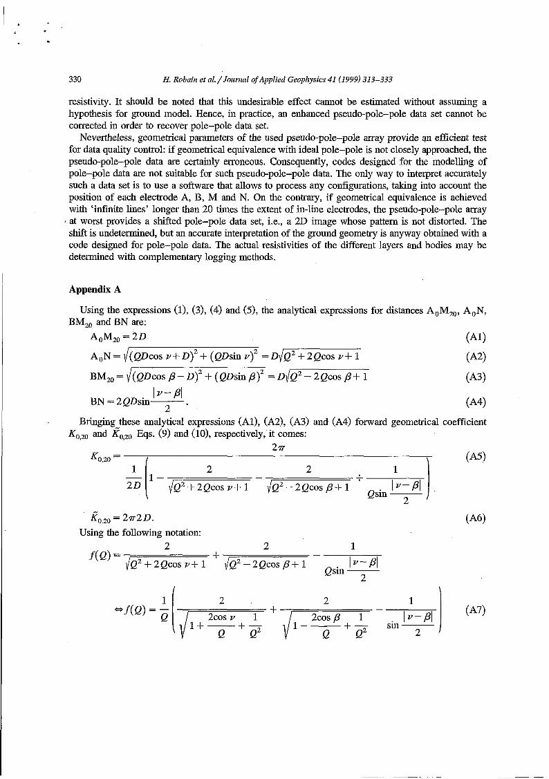
resistivity. It should be noted that this undesirable effect cannot be estimated without assuming a hypothesis for ground model. Hence, in practice, an enhanced pseudo-pole-pole data set cannot be corrected in order to recover pole-pole data set.

Nevertheless, geometrical parameters of the used pseudo-pole-pole array provide qn efficient test for data quality control: if geometrical equivalence with ideal pole-pole is not closely approached, the pseudo-pole-pole data are certainly erroneous. Consequently, codes designed for the modelling of pole-pole data are not suitable for such pseudo-pole-pole data. The only way to interpret accurately such a data set is to use a software that allows to process any configurations, taking into account the position of each electrode A, B, M and N. On the contrary, if geometrical equivalence is achieved with 'infinite lines' longer than 20 times the extent of in-line electrodes, the pseudo-pole-pole array

8 at worst provides a shifted pole-pole data set, i.e., a 2D image whose pattern is not distorted. The shift is undetermined, but an accurate interpretation of the ground geometry is anyway obtained with a code designed for pole-pole data. The actual resistivities of the different layers and bodies may be determined with complementary logging methods. ,

Appendix A ~

Using the expressions (l), (3), (4) and (5), the analytical expressions for distances A,M,, A,N, BM,, and BN are:

A,M, = 2 0 (Al1

(W (A31

A,N = i( QDcos Y + O), + ( QDsin Y), = D{Q2 + ~ Q C O S Y+ 1

BM,, = {( QDcos ß - O), + ( QDsin ß), = 0{Q2 - 2Qcos ß + 1

I Y- ßl BN = 2QDsin-. 2

Bringing these analytical expressions (Al), (A2), (A3) and (A4) forward geometrical coefficient KO,," and Eqs. (9) and (lo), respectively, it comes:

21r KO,," =

1 I. 2 2 1 1 + - - I V - ß 1 J Qsin ~

2 0 1' - {Q2 + 2Qcos Y+ 1 {Q2 - 2Qcos ß+ 1 2

M

K",," = 2lr2D.

f ( Q ) =

Using the following notation: 1

Qsin -

- 2 2 + {Q2 + 2Qcos v + 1 {Q2 - 2Qcos ß + 1 I V - ß 1

2

1 W f ( Q > = - Q

. 4

H. Rohain et al. / Journal of Applied Geophysics 41 (1999) 313-333 331

and then replacing coefficients ICozo and f?o,20 by their expressions (AS) and (A6) in difference S( expression (1 l), it comes &ter simplifying and factorizing:

s(Ko,20) = loo( 1 - 1 ) = loo( f(Q) ). 1 -f(Q) f(Q) - 1

For x close to zero, the second order approximation of Taylor development gives:

a(a - 1) 2

(1 + X)O = 1 + m + X2.

Using approximation (Ag), it comes:

The terms 1/Q" with exponent n higher than 2 may be neglected, thus, Eq. (Alo) simplifies to:

With the same simplification, it comes:

(A121 1 1

= 1 + -cosß- Q

Bringing approximations (All) and (A12) forward f(Q) expression (A7) and regrouping 1/12" terms, gives the desired third order approximation:

1 1 +2 I+--- ---cos2ß - ( yß d.(: : 11 Sin - I V - ß 1

2

1 1

Q3 1 + $2(COS p- cos Y) - -(2 - 3(cos2 v+ cos2 p)). 4 -

. I V - ß 1

332 H. Rohain et al./ Journal of Applied Geophysics 41 (1999) 313-333

Appendix B

is calculated using Pythagore's formula for the triangle OiJ, Ny N' shown on Fig. 3:

( o , , ~ N ) ~ = ( N N ~ ) ~ + (o , ,~N ' )~ - ( o , , ~ N ) ~ = + ( O ~ , ~ O + Developing distances Oi,jN, NN' Oi,jO and ON' in Eq. (Bl), it comes:

2

(Qi,jDì,j)2 = (QDsin t)'+ (D( 1 - q) + QDcos i) , where n + 1 is the number of in-line electrodes.

The distance is defined as: A iMj D

= 2 then Did= ( j - i ) - . 11

Finally, replacing distance gives the desired Qj,j expression:

by its expression (B3) in Eq. (B2), simplifying and factorizing,

i + j QiJ = A{( Qsin g ) 2 + (1 - - y1 + Qcos !)'. 2

J - - 1

Bi,j is calculated using sinus definition: B

"i QDsin- . 'i., j 2

2 Oi,jN Qi,jDi,j sin - = - =

Replacing the term Qi,jDi,j with its expression (B2) in Eq. (B5) and simplifying gives the desired Bì,j expression:

= 2sin-'

e Qsin -

2

References

Barker, R.D., 1992. A simple algorithm for electrical imaging of the subsurface. First Break 10, 53-62. Beard, L.P., Tripp, A.C., 1995. Investigating the resolution of IP arrays using inverse theory. Geophysics 60, 1326-1341. Brunel, P., 1994. Dispositif multiélectrode en courant continu. Etude et application i des structures bidimensionnelles. Thèse

Cherry, P., Bruand, A., Arrouays, D., Dabas, M., 1996. Cokriging electrical resistivity for detailed study of soil thickness

Dabas, M., Tabbagh, A., Tabbagh, J., 1994.3-D inversion in subsurface electrical surveying: I. Theory. Geophys. J. Int. 119,

Griffiths, D.H., TurnbulL J., 1985. A multi-electrode array for resistivity surveying. First Break 3, 16-20. Griffiths, D.H., Turnbull, J., Olayinka, AI., 1990. Two-dimensional resistivity mapping with a computer controlled array.

Univ., Paris, 6.

variability: a case study in beauce area (France). EGS La Haye, Annales Geophysicae 12, C462, Supl. II.

975-990.

First Break 8, 121-129.

r p R

H. Rohain et al./ Journal of Applied Geophysics 41 (1999) 313-333 333

Griffiths, D.H., Barker, R.D., 1993. Two-dimensional resistivity imaging and modelling in areas of complex geology.

Guérin, R., Tabbagh, A., Andrieux, P., 1994. Field and/or resistivity mapping in MT-VLF and implication for data

Hallof, P.G., 1957. On @e interpretation of resistivity and induced polarization measurements, PhD thesis. Massachusetts

Harrington, R.F., 1961. Time Harmonic Electro-magnetic Fields. McGraw-Hill, New York, USA. Hesse, A., Tabbagh, A., 1986. New prospects in the shallow depth electrical surveying for archeological and pedological

Keller, G.V., Frischknecht, F.C., 1966. Electrical Methods in Geophysical Prospecting. Pergamon. Kunetz, G., 1966. Principles of direct current resistivity prospecting. Geoexploration Monographs Ser. 1, No. 1. Gebriider

Borntraeger Ed, Berlin-Nikolassee. Lamotte, M., Bruand, A., Dabas, M., Donfack, P., Gabalda, G., Hesse, A., Humbel, F.X., Robain, H., 1994. Distribution

d’un horizon ‘a forte cohékion au sein d’une couverture de sol aride du Nord-Cameroun. Aport d’une prospection électrique. Comptes rendus ‘a l’académie des sciences. Earth and Planetary Sciences 318 (7), 961-968, Ser. II.

Loke, M.H., Barker, R.D., 1996. Rapid least-squares inversion of apparent resistivity pseudosections by a quasi-Newton method. Geophysical Prospectings 44,499-524.

Parasnis, D.S., 1997. In: Chapman et al. (Eds.), Principles of Applied Geophysics, 5th edn. London, UK. Robain, H., Descloitres, M., Ritz, M., Yene Atangana, Q., 1996. A multiscale electrical survey of a lateritic soil system in

Roy, A., Apparao, A., 1971. Depth of investigation in direct current methods. Geophysics 36, 943-959. Shima, T., 1990. Two-dimensional automatic resistivity inversion technique using alpha centers. Geophysics 55, 682-694. Tabbagh, A., 1985. The response of a three-dimensional ,magnetic and conductive body in shallow depth electromagnetic

Telford, W.M., Geldart, L.P., Sheriff, R.E., 1990. Applied Geophysics, Second edn. Cambridge Univ. Press.

Journal of Applied Geophysics 29, 211-226.

processing. Geophysics 59, 1695-1712.

Institute of Technology.

applications. Geophysics 51, 585-594.

the rain forest of Cameroon. Journal of Applied Geophysics 34, 237-253.

prospecting. Geophys. J. R. Astr. Soc. 81 (l), 215-230.