The Liquidity Effect in the Federal Funds Market: Evidence ... · The Liquidity Effect in the Federal Funds Market: Evidence from Daily Open Market Operations Seth Carpenter and Selva

Finance and Economics Discussion Series Divisions of Research & Statistics and Monetary Affairs

Federal Reserve Board, Washington, D.C.

The Liquidity Effect in the Federal Funds Market: Evidence from Daily Open Market Operations

Seth Carpenter and Selva Demiralp

2004-61 NOTE: Staff working papers in the Finance and Economics Discussion Series (FEDS) are preliminary materials circulated to stimulate discussion and critical comment. The analysis and conclusions set forth are those of the authors and do not indicate concurrence by other members of the research staff or the Board of Governors. References in publications to the Finance and Economics Discussion Series (other than acknowledgement) should be cleared with the author(s) to protect the tentative character of these papers.

The Liquidity Effect in the Federal Funds Market: Evidence from Daily Open Market Operations

Seth Carpenter and Selva Demiralp

Division of Monetary Affairs The Board of Governors of the Federal Reserve System

September 2004

Abstract

We use forecast errors made by the Federal Reserve while preparing open market operations to identify a liquidity effect at a daily frequency in the federal funds market. Unlike Hamilton (1997), we find a liquidity effect on many days of the reserve maintenance period besides settlement day. The effect is non-linear; large changes in supply have a measurable effect but small changes do not. In addition, a higher aggregate level of reserve balances in the banking system is associated with a smaller liquidity effect during the maintenance period but a larger liquidity effect on the last days of the period.

The views expressed are those of the authors and do not necessarily reflect those of the Board of Governors, the Federal Reserve System, or other members of the staff. We thank Heather Wiggins and Shawn Liu for research assistance. We also thank Dennis Farley, Sherry Edwards, and seminar participants in the Division of Monetary Affairs, and staff at the Domestic Money Market Desk at the Federal Reserve Bank of New York for helpful comments. Carpenter: Mail Stop 60, 20th and C Street, NW Washington, DC 20551 [email protected], Demiralp: Mail Stop 59, 20th and C Street, NW Washington, DC 20551 [email protected]

2

I. Introduction

The ability of the Federal Reserve to control the federal funds rate is taken for

granted. Each morning, the trading desk (the Desk) at the Federal Reserve Bank of New

York (FRB-NY) conducts open market operations to adjust the supply of reserves in the

banking system in order to achieve the target for the funds rate set by the FOMC. This

manipulation of reserves to affect the funds rate relies on a presumption of a liquidity

effect. Specifically, it is assumed that a greater supply of reserves will tend to cause the

funds rate to fall ceteris paribus, and likewise, a reduction in the supply of reserves will

tend to cause the funds rate to rise.

Hamilton (1997) tested whether this relationship exists at the daily frequency.

His results suggest that a significant liquidity effect exists at the daily level only on

“settlement Wednesday.” That is to say, on the last day of the bi-weekly periods over

which banks must satisfy their reserve requirements. In a reinterpretation of Hamilton’s

work, Thornton (2001) suggests that the evidence is questionable. He argues that

Hamilton’s results rely primarily on a small number of observations with large

movements in the funds rate. Excluding these observations, Thornton does not find

evidence of a daily frequency liquidity effect. Previous researchers (e.g. Reichenstein

(1987), Leeper and Gordon (1992), Strongin (1995)), analyzing lower frequency data,

have noted a similar lack of correlation between monetary aggregates and various interest

rates, calling this the “liquidity puzzle.”

In this paper, we present strong empirical support for a daily liquidity effect.

Moreover, we find evidence of the liquidity effect on several days within the maintenance

period, not simply on settlement Wednesdays. Building on these results, we examine

some determinants of the magnitude of the liquidity effect. We find that appropriately

3

defined “small” exogenous changes in the supply of reserves do not have a statistically

significant effect on the funds rate whereas “large” changes in reserves do, suggesting a

non-linearity in the liquidity effect. Next, we ask what effect the aggregate level of

reserve balances in the system has on the liquidity effect. We find evidence that higher

levels of reserve balances lead to an attenuated liquidity effect in the middle of the

maintenance period, but a stronger liquidity effect at the end of the maintenance period.

The supply of Fed balances is determined by the Desk’s open market operations,

discount window lending, and the movements in autonomous factors on the Fed’s

balance sheet. Autonomous factors consist of Federal Reserve assets and liabilities over

which the Desk has little or no control. Hamilton used errors in forecasts of one of these

autonomous factors, the Treasury’s balance at the Federal Reserve, to identify exogenous

shifts in the supply of reserves. While in principle this approach is valid, the forecasts are

made from historical data, and thus do not necessarily correspond to actual daily

exogenous changes in reserves. Hamilton would like to have an unbiased estimate of the

level of reserves in the banking sector that is consistent with the funds rate at the target

rate and estimate the effect on the funds rate when the realized value deviates. However,

he has one imperfect measure of only one factor affecting the supply of reserves in the

market. We propose a more accurate and more complete measure.

Each morning, staff at the Federal Reserve Bank of New York and the Board of

Governors make a forecast of all of the factors that affect the supply of reserves in the

market. Conditional on these forecasts, the Desk performs an open market operation to

equate the supply of reserves with the quantity of reserves that would be demanded that

day at the target funds rate. In other words, there is an implicit model of a negatively

4

sloped demand curve and a vertical supply curve, with supply adjusted to achieve

equilibrium at the target rate.

In evaluating the daily demand for reserves, the Desk considers various factors

such as the day of the maintenance period, days when payment-related flows are likely to

be elevated, etc. (see Demiralp and Farley (2004) for a detailed discussion of the

determinants of daily open market operations). This implies that the quantity of reserves

supplied to the market is shifted to account for daily changes in the demand for reserves.

When there is a mismatch between the Desk’s forecast of the supply of reserves and the

actual supply of reserves that is realized in the banking system, the difference—or

forecast miss—is an exogenous shift in the supply of reserves. We use the daily forecast

miss to identify exogenous shifts in the supply of reserves.1 Because the Desk achieves

the target rate on average, the correlation between the daily forecast miss and the

deviation of the funds rate from the target allows us to estimate the liquidity effect at the

daily frequency.

Under our identification scheme, we estimate a statistically significant negative

relationship between changes in the supply of reserves and the federal funds rate. We

find that many, but not all, days within a maintenance period exhibit a liquidity effect.

Echoing Hamilton’s findings, the effect is particularly strong on settlement Wednesday.

We believe our measure is superior to Hamilton’s measure in that it is not based on an

estimate of a reserves miss, but is the reserves miss itself. Moreover, we find that the

results are statistically significant after 1994 when the Federal Reserve began announcing

changes to the target rate. It has been speculated, for example by Thornton (2001) that

1 More specifically, we take the Board staff forecast to calculate the miss. As a robustness check, we also use the forecast miss from the FRB-NY and the average of the two. The results are essentially the same.

5

following the announcement of the target, manipulation of reserves was no longer needed

to maintain the funds rate target and thus there ought not be a liquidity effect. In contrast,

we find that the liquidity effect is evident in the post-1994 sample. In fact, if there is a

downward sloping demand curve for reserves, so-called “open mouth operations” would

only be able to change the funds rate to the new target by shifting the demand curve

through expectations of a different future rate, while a manipulation of reserves would

still be required to maintain the target. In this respect, our results are not inconsistent

with the view that announcement effects are important in the daily market.

The following section lays out an overview of the literature on the liquidity

effect, putting the current work into context. The next section explores the federal funds

market in some detail and explains the institutional characteristics that allow us to

identify shifts in the supply of reserves. Next, we present our empirical specification and

our results. The final section concludes, drawing comparisons between the current work

and previous work, as well as the results from a related paper on the liquidity effect at the

monthly frequency.

II. The Liquidity Effect and the so-called Liquidity Puzzle

Generally speaking, the liquidity effect is a negative relationship between a

measure of money and an interest rate. The economics literature has no shortage of

papers that investigate this type of relationship, including e.g. Cochrane (1989), Gali

(1992), Leeper and Gordon (1992), Strongin (1995), Pagan and Robertson (1995),

Christiano (1991), Bernanke and Mihov (1998), Hamilton (1997), and Thornton (2001).

The methodologies and the results are mixed; some researchers have not found a

consistent relationship—the “liquidity puzzle”—while other researchers have.

6

At the heart of all the analysis is a demand curve for some type of money that in

principle depends negatively on an interest rate. The liquidity effect, then, can be thought

of as directly related to the slope of this demand curve. Leeper and Gordon (1992),

Pagan and Robertson (1995), and others have used a monetary aggregate (M1 or M2) and

an open market interest rate (such as the yield on the three-month Treasury bill) to test for

the liquidity effect. The fact that results are not robust in this setting is taken to be a lack

of evidence for a liquidity effect. However, money demand models for the aggregates are

notoriously unstable. Furthermore, changes in broad monetary aggregates are likely to

suffer from an endogeneity problem where they embody policy accommodation of

demand in addition to exogenous shifts in demand. As a result, failure to estimate a

liquidity effect could simply be a misspecification or a shifting of an underlying demand

function.

Strongin (1995), Bernanke and Mihov (1998) and others specifically interested in

the transmission mechanism explicitly model the federal funds market to estimate a

liquidity effect. In particular, Strongin notes that the failure of other researchers to find a

liquidity effect can be traced, at least in part, to a failure to account for the Federal

Reserve’s accommodation of shifts in the demand for money or reserves. Bernanke and

Mihov point out that testing for a liquidity effect with monetary aggregates is

inappropriate for similar reasons. Explicitly modeling the market of nonborrowed

reserves, these researchers find a significant liquidity effect at the monthly frequency.

This set of results is closely linked to results in Carpenter and Demiralp (2004)

who also find strong evidence of a liquidity effect at the monthly frequency. That study,

however, also highlights the importance of understanding why a liquidity effect may not

be present. They note that, looking at contemporaneous correlations, there is a liquidity

7

effect with respect to total reserve balances and the federal funds rate. This relationship

however, does not hold when only nonborrowed reserves are studied. Because reserve

requirements are determined by a bank’s customers’ demand for reservable deposits,

which may or may not depend on the funds rate in a simple way, there is no reason to

expect a liquidity effect between nonborrowed reserves and the funds rate in periods

when required reserve balances constitute the majority of banks reserve balances.

In his influential work, Hamilton (1997) presents an empirical model of the funds

market at the daily frequency and attempts to estimate a liquidity effect. The Treasury

maintains an account with the Federal Reserve and each day funds are transferred in and

out of this account. As funds are transferred in, they are drained from the banking sector,

and thus the federal funds market. Hamilton exploits this relationship and estimates a

forecasting equation for the Treasury’s Fed account. If this forecasting equation is

unbiased, then deviations from the forecast ought to, on average, represent exogenous

shifts in the supply of reserves, allowing him to identify the liquidity effect. Hamilton’s

results suggest that there is a liquidity effect at the daily frequency, however the effect is

only statistically significant on the last two days of a maintenance period. Moreover, the

point estimate for the penultimate day of the maintenance period is not economically

significant. Hamilton’s work suggests a liquidity effect, but a very specific one, confined

to the last day of a maintenance period.

Thornton (2001) re-examines Hamilton’s results and argues that the liquidity

effect cannot be identified because it is almost impossible to correctly identify the error

that the Fed makes in forecasting the Treasury balance. Moreover, Thornton finds that

Hamilton’s settlement Wednesday result is “fragile and it arises due to a few settlement

8

Wednesdays when there were unusually large changes in the funds rate.” Thornton goes

on to argue that the liquidity effect can be identified by examining changes in

nonborrowed reserves following a change in the target rate. He concludes that the

quantities of changes in nonborrowed reserves are relatively small, and thus likely are

only signals of a change in target, but not evidence of a liquidity effect itself.

In this paper, we follow these two researchers in examining daily data. In the

next section, we explain the daily forecasting and operation procedures of the Federal

Reserve and argue that the difference between the actual supply of reserves on a day and

the forecast used in determining open market operations provides an exogenous shift in

the supply of reserves in the funds market.

III. The federal funds market and the supply of reserves

The Desk at FRB-NY conducts open market operations, in an attempt to equalize

the demand for and supply of reserve balances in the banking sector at the target federal

funds rate. Demand for reserves comes from two primary sources, clearing needs and

reserve requirements. Because banks use their Federal Reserve accounts to clear

transactions for themselves and their customers, the demand for reserves tends to be

higher on days with large expected volumes of payments, such as month-, quarter-, and

year-end. In addition, over a two-week maintenance period, banks are required to hold,

on average, a quantity of reserves at the Fed proportional to the quantity of transactions

deposits at the bank over the previous two-week computation period. Demand for

required reserve balances, therefore, can be easily substituted across all fourteen days in a

maintenance period, however balances held on a Friday are carried over for both

9

Saturday and Sunday. Similarly, starting in 1981 under the Monetary Control Act, banks

are able to establish contractual clearing balances with their Federal Reserve Bank,

agreeing in advance to maintain a specified level of balances, above and beyond their

reserve requirements. In exchange for committing to hold these balances, banks are paid

a form of implicit interest on the contractual clearing balances. Specifically, banks are

given credits applicable to priced services they receive from their Federal Reserve Bank,

and these credits until January 2004 were tied to the funds rate that prevailed over the

maintenance period and since then are tied to a fraction of the three-month Treasury bill.

As can be seen in Figure 1, total reserve balances, the sum of required reserve

balances, contractual clearing balances, and excess balances, have declined on average

over the past decade. This decline is due to several factors including decreases in

required reserve ratios and the advent of “sweep accounts” whereby banks move deposits

from reservable demand deposits into savings accounts that have a reserve requirement of

zero. Because this shift has taken place through time, it is unlikely to have much of an

impact on our estimation of the daily frequency liquidity effect.

Excluding contractual clearing balances, reserve balances do not earn any interest.

Therefore, banks would like to minimize their holdings of excess reserve balances except

to avoid a costly overdraft of their account. For that reason, given the intra-maintenance

period substitutability of reserve balances, banks are somewhat hesitant to hold large

balances of reserves early in the maintenance period. Figure 2 presents the average

pattern of excess reserve balances over a maintenance period from 1989 to present.

Banks are often deficient in their reserve requirements early in a maintenance period

where their primary objective is to meet their payment-related balances that they must

10

hold to avoid overnight overdrafts. They make up the deficiency in the latter part of the

period when they have better information about their period-average reserve needs and

still satisfy their requirements.

In the context of a simple model, we think of the demand for reserve balances, td ,

as a function:

d ff Xt t t t, (1)

where tff is the federal funds rate and X t is the set of all other variables that affect

demand like the day of the maintenance period or days of heavy transaction flows, and t

is a random error term. Note that we do not consider the function to necessarily be linear

or separable among these variables.

Each morning, staff at FRB-NY and at the Board of Governors in Washington,

D.C. make forecasts of all the factors that affect the supply of reserves. The most

important among these factors are currency, check float, and the Treasury’s balance at the

Fed. Currency is introduced into circulation when banks request a shipment from their

Federal Reserve Bank. The value of the currency shipment is then debited from the

bank’s reserve account. Thus, in times of higher public demand for currency, ceteris

paribus, reserves are drained from the system. During the processing of checks, there are

occasionally delays in the presentation of checks to banks on which they are drawn. As a

result, check float can be created if the receiving bank has been credited before the

drawing bank is debited. In this case, reserves in the banking system would be increased

until the double counting is undone. Conversely, if the paying institution’s account is

11

debited faster than the schedule for crediting the receiving institution’s account, reserve

balances are reduced. As discussed above, the Treasury maintains an account at the

Federal Reserve, from which all federal payments are made. When a payment is made

out of this account, funds are transferred from the Treasury account into the reserve

account of the receiving bank. As a result, payments from the Treasury account increase

reserve balances and receipts to the Treasury account drain reserve balances. Note that

this effect on reserve balances does not depend on the recipient/payer of the funds. When

a private citizen pays his/her taxes, for example, the check used for payment is drawn on

a bank. When the check is processed, the bank’s reserve account is debited.

With an assessment of the level of demand and a forecast of the factors affecting

the supply of reserves, a decision over the size of the needed open market operation for

the day is made. On average in our sample, the funds rate is equal to the target rate,

therefore we take as a maintained hypothesis that over time the quantity of reserve

balances supplied equals the quantity of reserve balances demanded at the target rate.

Thus, we also assume that the Desk correctly infers the demand function, an assumption

we are able to test below.

The supply of reserve balances on a given day, ts , is fixed and equal to the sum of

the factors affecting the supply of reserves, f t and the daily open market operation, omot

or:

s f omot t t (2)

12

In terms of these simple supply and demand functions, the liquidity effect is

essentially a negatively sloping demand curve, or / ff t 0. To attempt to estimate

this effect, consider a simplified, linear version of the demand and supply curves.

t t t td X ff (3)

1wheret t t t t t ts f omo f E f miss (4)

Where 1tE is the expectations operator conditional on an information set as of time

1t , and tmiss is the forecast error on day t. The intended quantity supplied is adjusted

to be equal to the expected quantity demanded, evaluated at the target rate, ff t* , subject to

the fact that the Fed has only estimates of the parameters of the demand function:

^ ^*

1t t t t tE f omo X ff (5)

In equilibrium, supply must equal the demand for reserve balances. Substituting tf into

(5) and moving total factors miss to the right hand side:

^ ^*X ff miss X fft t t t t t

(6)

Re-arranging (6) we get the following equation:

* *ˆ ˆ 1 1( )t t t t t tff ff ff X miss(7)

This equation merits a few comments and will be the basis for our more general empirical

specification elaborated in the next section. First, and foremost, the coefficient on the

13

daily forecast miss allows us to test for a daily frequency liquidity effect as it is the

reciprocal of the partial derivative of the demand for balances with respect to the funds

rate. Econometrically, this should be a valid test because the forecasts are made by staff

at the Federal Reserve about factors affecting the supply of reserves and are not related to

random fluctuations in banks demand for reserve balances. Thus, they should be

uncorrelated with the error term. The set of variables tX represents the set of variables

that shift the demand for reserve balances on a daily basis. If the Desk estimates these

daily fluctuations in demand accurately, then the coefficients will be equal to zero,

otherwise the dummy variables will soak up these daily disturbances. Lastly, the

equation suggests including the target level of the federal funds rate into the specification.

This coefficient will provide a test about whether or not, on average, the level of the

target generates a systematic bias in the deviations from the target. Further, a statistically

significantly negative (positive) coefficient implies that the Desk under- (over-)estimates

the slope in the underlying function.

IV. Empirical Specification

IV-1. Data

Data on the daily effective funds rate are published in the Federal Reserve’s H.15

statistical release. This rate is the weighted-average interest rate paid on overnight funds

traded in the brokered federal funds market. Beginning in 1994, the Fed began

announcing changes in its target for the federal funds rate. In general, but not always,

these changes have occurred at FOMC meetings. The data on daily forecast misses come

14

from internal databases maintained at the Board of Governors. We use forecast misses

from the Board of Governors.

IV-2. Specification

While the simple model outlined in the previous section assumed that the demand

for reserve balances was strictly linear and separable in the funds rate and other factors

that affect demand, we relax that assumption somewhat to be able to test for intra-

maintenance period variation in the liquidity effect. In addition, we estimate an

exponential GARCH specification (Nelson (1991)) for the deviation of the funds rate

from the target rate in order to allow for conditional heteroscedasticity in the error term.

High payment flow days may shift the demand for funds, but they also instill greater

uncertainty in the market and influence daily volatility that we wish to model. The

EGARCH specification further allows for asymmetry in volatility as defined by the

variance of the error term, 2 .

2 21 1

1

1 1

* * *1 1 1 1 2 2 1 1

log log

( ) *

t tt t

t t

t t t t t t t t t t t

t tZ

ff ff D ff ff D ff ff mpday mpday miss CX (6)

Where iD is a dummy variable corresponding to the i=1,2 week of the maintenance

period. We include the daily forecast error, miss, interacted with dummies corresponding

15

to each day of the maintenance period, tmpday . In addition, we include a set of variables

to control for daily shifts in the demand for reserve balances, these are:

A dummy variable for each day of the maintenance period.

A dummy variable for month-ends, quarter-ends, and year-ends, respectively.

A dummy variable for the first day of a month, quarter, and year, respectively.

A dummy variable for the 15th of a month.

Dummy variables for the day before and the day after a holiday, respectively.

An interaction of a dummy for the day before a target change and the anticipated change in the target rate as implied by fed funds futures contracts.

An interaction of a dummy for the day of a target change and the unanticipated change in the target rate as implied by fed funds futures contracts.

A dummy variable for the month of December.

The target for the federal funds rate.

The variance equation has the following variables:

EGARCH terms.

A dummy variable if the observation is in the last three days of a maintenance period.

Dummy variables for the first and the second Fridays of a maintenance period.

A dummy variable for the day before and after a change in the target rate, respectively.

A dummy variable for the day before and after a holiday, respectively.

A dummy variable for month-, quarter, and year-end.

A dummy variable for the month of December.

16

V. Results

V-1. Basic results

The results of the estimation are presented in Table 1. The sample period covers

May 19, 1989 through June 27, 2003. The starting point of our sample corresponds to the

establishment of the Fed funds futures market at Chicago Board of Trade. Columns 2 to

4 present full-sample results. In order to check whether the period after February 1994,

display a change in parameters, we also present the results for this latter period in

columns 5 to 7.

A likelihood ratio test of the hypothesis that all of the coefficients of the miss

interacted with the days of the maintenance period are zero is rejected at the 1%

confidence level. We consider this negative and statistically significant coefficient to be

clear evidence of a liquidity effect at the daily frequency. In examining these coefficients

more closely, however, interesting patterns emerge.

Corroborating Hamilton (1998), we find the largest liquidity effect is on

settlement Wednesday. Banks must fulfill their reserve requirements by settlement

Wednesday; deficiencies cannot be shifted to later days except for a small carry-over

allowance.2 Thus, deviations in supply from the quantity demanded on these days appear

to have the largest impact on the funds rate. Taken at face value, it would appear that a

change of a billion dollars in reserve balances is sufficient to move the funds rate by

almost 3-1/2 basis points on settlement Wednesday.

2 The reserve carry-over privilege provides a depository institution with some flexibility in meeting its total balance requirement. This privilege allows an institution with a small excess or deficiency (maximum carry-over allowance is the greater of four percent or $50,000) in one maintenance period to use it or make it up in the following maintenance period.

17

In contrast to Hamilton’s findings, with the exception of three days—the first two

days of the maintenance period and the second Friday—each day of the maintenance

period displays a statistically and economically significant liquidity effect for the full

sample. The penultimate day of the maintenance period and both Mondays (days 3 and

8) have the next largest point estimates, however, several of the other coefficients imply a

non-trivial response of the funds rate to changes in the supply of reserve balances.

Averaging coefficients across days of the maintenance period suggest that a change of $1

billion in reserve balances could move the funds rate by about 1 basis point.

The first day of the maintenance period does not display a significant liquidity

effect. Recalling a bank’s demand for reserve balances (Figure 2), this may be expected.

In the beginning of a maintenance period, a bank has a relatively long horizon to adjust

its maintenance period average reserve balances to fulfill its requirements. Thus, the

slope of the demand curve is steepest on Thursday, and changes in reserve balances elicit

less of a funds rate reaction as banks are more able to intertemporally shift reserve needs.

As the maintenance period progresses, this ability is diminished and thus the liquidity

effect is stronger later in the maintenance period. Of curiosity, however, is the large

estimated coefficient on the first Monday of the maintenance period. While this day

ought to have almost as little sensitivity as the two previous days, recall that Friday

balances are counted three times. As a result, although demand for reserves on the first

Friday of a maintenance period may not be especially sensitive, on the subsequent

Monday, once the reserve position for the previous Friday has been realized, banks may

attempt to unwind some of the three-day effect from the weekend.

18

The columns 5 to 7 of Table 1 presents the regression results using data since

1994, the year the Fed began announcing changes to the target rate. The results are

qualitatively similar to Hamilton (1997) and our results over the longer sample. The

liquidity effect on settlement Wednesday appears to be a bit smaller than the full-sample

results, but most other coefficients are perhaps a touch larger, and all but one of the days

of the maintenance period exhibit a statistically and economically significant liquidity

effect. Thornton suggested that so-called open mouth operations may be an explanation

for his not finding a liquidity effect. The logic is that the Fed is able to control the funds

rate near the target rate simply by announcing the target and thus the supply of reserve

balances is incidental to the funds rate. We disagree with this logic and our results do not

support Thornton’s conclusions. We believe that the announcement effect associated

with open mouth operations is significant in changing the funds rate following a target

change, as shown by the insignificant liquidity effect associated with factors misses on

the day after a target change. However, the “announcement effect” only operates on the

day after a target change and on the remainder of the days in our sample, maintenance of

the target does require careful reserve management through open market operations. It

should also be noted that it is the credibility of the Trading Desk in its commitment to the

target rate that establishes market expectations and enables the announcement effect.

One interesting note is the estimated coefficient on the target funds rate. In both

specifications, the point estimate is small and p-value ranging between .1 and .3;

essentially the coefficient is zero. This implies, given our theoretical results above, that

the Desk at the FRB-NY has been able to understand, on average and through time, the

relationship between the demand for reserve balances and the federal funds rate. There is

19

no evidence of systematic mis-estimation of the elasticity. Meanwhile, the coefficients

associated with the set of variables that represent demand for balances are mostly

significant, suggesting that the Desk does not completely offset these daily fluctuations in

demand.

Finally, the positive and significant coefficient in the conditional variance

equation indicates that the volatility effects of upward and downward moves in the funds

rate are asymmetric, consistent with Hamilton (1996). An upward funds rate shock leads

to greater volatility in the funds market than a downwards shock. Most of the other

coefficients in the variance equation are significant and positive, except for the first

Friday of a maintenance period when the volatility tends to be lower, likely due to a

lower volume of trading. This finding is somewhat different from Spindt and

Hoffmeister (1988) who find that the variance of the funds rate increases on both Fridays

and especially on the second Friday. This result likely reflects a change in trading

patterns since the period between 1984-1986, when the above results were obtained.

V-2. Non-linear liquidity effect

We next ask whether the liquidity effect that we identified above is linear in the

miss. Specifically, we define a miss of $1 billion or more to be a large miss and test

whether the coefficient on large misses is the same as the coefficient on small misses.3

Our sample consists of roughly 1/3 large misses and 2/3 small misses, implying that we

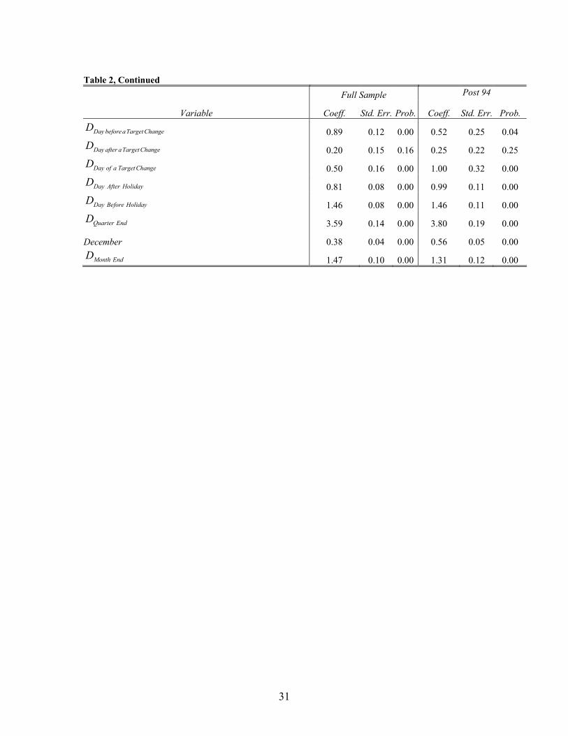
have sufficient power to test our hypothesis. The results are presented in Table 2 with

3 The sample standard deviation of the forecast misses is $1.1 billion, providing a less-arbitrary justification for our choice of large versus small.

20

results for the post-1994 sample in the right column for comparison. These results

suggest that the liquidity effect at the daily frequency is non-linear. The coefficients on

small misses are statistically insignificantly different from zero for most days while the

coefficients on large misses are generally larger than our results presented in Table 1.

From these results, we conclude that the federal funds market is insensitive to small

deviations from equilibrium. Put in slightly different terms, the demand curve for funds

appears to be kinked, and roughly flat in the neighborhood of the target rate. One

interpretation for this result is that the loss to a bank of a small deviation from its optimal

choice for reserves on a given day is smaller than the transactions costs required to adjust

its balances. This situation is reinforced by the fact that funds held to satisfy reserve

requirements across different days of the maintenance period are perfectly substitutable.

This result further helps to reconcile our findings with those of Hamilton and Thornton.

Thornton asserts that Hamilton’s results rely entirely on a handful of outliers. Our data

allow us to identify a differential effect of a small miss from a large miss, suggesting that

these outliers are, in fact, driving Hamilton’s results, but that the imprecision in his

instrument obscures the more general liquidity effect.

V-3. The effect of the level of operating balances

Next, we ask whether the level of operating balances in the banking system is

related to the size of the liquidity effect. Clouse and Elmendorf (1997) argue that for

sufficiently low levels of operating balances, the federal funds market can become

volatile. This concern was particularly acute as declines in required reserve ratios and the

increased use of retail sweep activity dramatically lowered required reserves to a point

where many banks were able to satisfy reserve requirements with vault cash. In the

21

context of the liquidity effect, we would suspect that a steeper demand curve for funds

would result in a more volatile funds market. In other words, if the federal funds rate is

more sensitive to changes in the quantity of reserves, a given miss in the supply of

reserve balances would result in a larger deviation of the funds rate from the target.

To test this hypothesis, we interact the daily forecast miss with a measure of the

aggregate level of required operating balances. We take the sum of required reserve

balances and contractual clearing balances, subtract the sample mean and then divide by

the sample standard deviation, normalizing the level of required operating balances to a

variable with a mean of zero and a standard deviation of unity.

The results are presented in Table 3, again with the post-1994 sample in the right

column. We find that a higher level of required operating balances tends to attenuate the

intra-maintenance period liquidity effect while it augments the end-of-maintenance

period liquidity effect. In essence, a higher level of required balances allows banks to

smooth deviations from their optimal choice of reserves across days of the maintenance

period more easily. However, at the end of the maintenance period, the need to fulfill a

higher requirement causes the funds rate to become more sensitive to deviations in

supply.

A specification that includes both the differentiation between large and small

misses, as well as interacting the results with the level of required operating balances is

consistent with the discussion above and suggests that the two phenomena we document

are independent effects.

22

VI. Conclusions

The results presented above are fairly strong evidence of a liquidity effect at the

daily frequency. Hamilton’s work on the daily liquidity effect is broadly consistent with

these results, however, his results suggest a statistically significant liquidity effect only

on the last day of the maintenance period. Our results differ from Hamilton’s in a

number of ways. It seems plausible that part of the difference between our results and his

is the difference in our measure of exogenous changes in the supply of reserves.

Hamilton created a forecast of only one factor affecting the supply of reserves and

compared it to the realized level of that factor. While in principle, the logic behind this

identification is sound, it seems likely that there is a great deal of estimation error and

imprecision in the method. Instead, we use the errors from the forecasts of all the factors

affecting the supply of reserves made by Federal Reserve in the actual conduct of

monetary policy. As a result, and given the theoretical and empirical results, our

approach provides a much cleaner and direct measure of exogenous changes to the supply

of reserve balances and likely explains some of the difference in the results.

In addition, the liquidity effect that Hamilton estimates is significantly larger than

ours. Indeed, he estimates that a change in reserve balances of $1 billion results in a

change in the funds rate of more than 22 basis points. For strictly day-to-day

fluctuations, this elasticity seems very large by recent standards. Over our sample period,

the deviation of the federal funds rate from the target has been approximately 3 ½ basis

points. Such small deviations suggest that the funds rate is no longer so sensitive to small

variations in reserve balances, a notion borne out by our examination of small versus

large misses.

23

Another major difference is the fact that we are able to estimate a statistically

significant liquidity effect on most days of the maintenance period. Lastly, Hamilton

estimates his model over a relatively short sample, from 1989 to 1991. Our sample

includes this period, but is longer and more recent and consequently, we feel that our

results are more representative of the current working of the market. Moreover, we

document that the liquidity effect tends to be larger at the end of the maintenance period

when required operating balances are higher. Recalling Exhibit 1, Hamilton’s sample

period is a period of extremely high operating balances. Our results would predict a

smaller liquidity effect early in the maintenance period and a larger effect later in the

period, suggesting that our results and Hamilton’s are not dramatically at odds.

The results of our paper, however, are quite different from those of Thornton. He

states

“[t]he demand for excess reserves is not well defined within the maintenance period because banks are free to alter their reserve holdings within the maintenance period so long as they hold enough reserves on a daily average basis to meet their requirement. Excess reserves become increasingly meaningful as the maintenance period draws to a close . . . even if the concept of the daily demand for excess reserves were meaningful, day-to-day fluctuations in excess reserves would likely be unpredictable.”

While Thornton’s point is valid, it nevertheless appears that there is a systematic pattern

of excess reserve balances within maintenance periods. Accordingly, our results suggest

that the sensitivity of reserve balances to changes in the interest rates does increase

through the maintenance period, though perhaps not strictly monotonically.

Thornton’s work is in line with some of the previous work on the liquidity effect

because, as he states, “the liquidity effect depends on the demand for money and not

banks’ demand for excess reserves.” Unfortunately, this logic implies a bit of the

24

mismatch we discussed in the second section of the paper. If money, e.g. demand

deposits, is not tightly linked to the federal funds rate, there is no reason to suspect that a

liquidity effect would be present there. However, as we discussed in the theoretical

section and as our empirical results confirm, there is a relationship between overall

reserve balances and the funds rate.

Furthermore, we find that the liquidity effect is non-linear. Specifically, small

deviations from the target supply of reserves in the banking system do not appear to have

a significant effect on the federal funds rate whereas large deviations do. This fact,

combined with Hamilton’s use of a noisy measure of supply shocks, reconciles our work

with previous work in the literature. Finally, we also find evidence that a higher level of

reserve balances in the banking system is related to a smaller liquidity effect during the

maintenance period, but an elevated liquidity effect at the end of the maintenance period.

In summary, our results provide solid evidence of a liquidity effect at the daily

frequency. We believe our data and methodology are more precise than Hamilton’s

seminal work. As a result, our results are broadly consistent with his work, but are

somewhat stronger.

25

References

Bernanke, B. and I. Mihov (1998), “The Liquidity Effect and Long-run Neutrality,” Carnegie-Rochester Conference Series on Public Policy, 49 pp. 149-194.

Bernanke, B. and I. Mihov (1998), “Measuring Monetary Policy,” Quarterly Journal of Economics, 113, pp. 869-902.

Carpenter, S. and S. Demiralp (2003), “The Liquidity Effect in the Federal Funds Market:Evidence at the Monthly Frequency,” unpublished manuscript Board of Governors of the Federal Reserve.

Christiano, L. (1991), “Modeling the Liquidity Effect of a Money Shock,” Federal Reserve Bank of Minneapolis Quarterly Review, Winter.

Clouse, J., and D. Elmendorf (1997), “Declining Required Reserves and the Volatility of the Federal Funds Rate,” Finance and Economics Discussion Series 1997-30, Board of Governors of the Federal Reserve System.

Cochrane, J. (1989), “The Return of the Liquidity Effect: A Study of the Short-Run Relation Between Money Growth and Interest Rates,” Journal of Business and Economics Statistics, 7, pp. 75-83.

Demiralp, S. and D. Farley (2004), “Declining Required Reserves, Funds Rate Volatility, and Open Market Operations,” Journal of Banking and Finance, (forthcoming).

Gali, J. (1992), “How Well does the IS-LM Model Fit Postwar US Data?” QuarterlyJournal of Economics, 107, pp. 709-738.

Hamilton, James (1996.) The Daily Market for Federal Funds. Journal of Political Economy 104: 26-56.

Hamilton, J. (1997), “Measuring the Liquidity Effect,” American Economic Review,March, 87(1), pp. 80-97.

Leeper, E. and R. Gordon (1992), “In Search of the Liquidity Effect,” Journal of Monetary Economics, 29, pp. 341-369.

Nelson, Daniel (1991.) Conditional Heteroskedasticity in Asset Returns: A New Approach,” Econometrica 59: 347-370.

Pagan, A. and J. Robertson, (1995), “Resolving the Liquidity Effect,” Federal Reserve Bank of St. Louis Review, 77, pp. 33-54.

Reichenstein, W (1987), “The impact of money on short term interest rates,” Economic Inquiry XXV, pp. 67-82.

26

Spindt, Paul and J. Hoffmeister (1988.) The Micromechanics of the Federal Funds Market: Implications of day-of-the-week Effects in Funds Rate Volatility. Journalof Financial and Quantitative Analysis 23 (4): 401-416

Strongin, S. (1995), “The Identification of Monetary Policy Disturbances: Explaining the Liquidity Puzzle.” Journal of Monetary Economics, August, 35(5), pp. 463-397.

Thornton, D. (2001), “Identifying the Liquidity Effect at the Daily Frequency” Federal Reserve Bank of St. Louis Review, July/August, pp. 59-78.

Table 1 Dependent Variable: (Deviation From Target)t Sample Period: May 18, 1989-Jan 30, 2004

Full Sample Post-94 Variable Coeff. Std. Err. Prob. Coeff. Std. Err. Prob.

1 1( )t WeekDeviation from Target D 0.29 0.01 0.00 0.28 0.02 0.00


( ) First ThursdayForecast Miss D -0.58 0.85 0.50 -0.75 0.90 0.40

( ) First FridayForecast Miss D 0.06 0.17 0.74 -0.62 0.30 0.04

( ) First MondayForecast Miss D -1.34 0.16 0.00 -2.57 0.19 0.00

( ) First TuesdayForecast Miss D -0.64 0.17 0.00 -0.62 0.21 0.00

( ) FirstWednesdayForecast Miss D -0.70 0.22 0.00 -0.99 0.29 0.00

( ) Second ThursdayForecast Miss D -0.49 0.26 0.06 -0.58 0.32 0.07

( ) Second FridayForecast Miss D -0.25 0.40 0.54 -0.25 0.46 0.60

( ) Second MondayForecast Miss D -1.33 0.59 0.02 -1.25 0.71 0.08

( ) Second TuesdayForecast Miss D -1.08 0.47 0.02 -0.75 0.44 0.09

( ) Second WednesdayForecast Miss D -3.41 0.67 0.00 -1.93 0.90 0.03

( ) Day after aTarget ChangeForecast Miss D -0.13 1.83 0.94 1.12 2.97 0.71

First ThursdayD 2.17 0.79 0.01 2.24 0.94 0.02

First FridayD -5.16 0.41 0.00 -4.32 0.56 0.00

First MondayD 4.04 0.34 0.00 2.63 0.55 0.00

First TuesdayD -2.01 0.41 0.00 -2.74 0.58 0.00

FirstWednesdayD -1.70 0.42 0.00 -1.13 0.55 0.04

Second ThursdayD 1.67 0.42 0.00 2.18 0.56 0.00

Second FridayD -4.05 0.45 0.00 -3.06 0.59 0.00

Second MondayD 4.54 0.92 0.00 3.83 1.05 0.00

Second TuesdayD -6.75 0.91 0.00 -7.50 1.09 0.00

Second WednesdayD 8.58 1.02 0.00 5.03 1.03 0.00

Month EndD 12.86 1.52 0.00 13.06 1.57 0.00

Month StartD 5.73 0.98 0.00 6.42 1.08 0.00

Quarter EndD 50.13 3.81 0.00 55.65 5.84 0.00

Quarter StartD 6.79 2.86 0.02 11.33 3.71 0.00

Year EndD -27.12 2.88 0.00 -39.06 4.08 0.00

28

Table 1, Continued.


Year StartD 17.28 6.88 0.01 5.76 6.54 0.38

Mid MonthD 10.17 0.34 0.00 9.21 0.44 0.00

Day Before HolidayD -2.57 1.10 0.02 -1.72 1.37 0.21

Day After HolidayD 11.06 1.13 0.00 13.09 1.46 0.00

1 1( )t t Day beforeaTarget Change WeekE Target D D 0.29 0.09 0.00 0.26 0.08 0.00


( )t Dayof aTarget ChangeUnanti D -0.63 0.08 0.00 -0.53 0.17 0.00 Target -0.07 0.06 0.26 -0.15 0.09 0.11

December -1.08 0.69 0.11 -0.64 1.01 0.53

Variance Equation Full Sample Post-94

Variable Coeff. Std. Err. Prob. Coeff. Std. Err. Prob.

C 1.05 0.05 0.00 1.25 0.07 0.00 |RES|/SQR[GARCH](1) 0.58 0.02 0.00 0.51 0.03 0.00 RES/SQR[GARCH](1) 0.04 0.02 0.03 0.06 0.02 0.01 EGARCH(1) 0.55 0.01 0.00 0.51 0.02 0.00

Last three daysof Maintenance PeriodD 1.43 0.04 0.00 1.18 0.05 0.00 First Friday -0.41 0.08 0.00 -0.52 0.09 0.00 Second Friday 0.19 0.05 0.00 0.11 0.06 0.05

Day beforeaTarget ChangeD 0.89 0.12 0.00 0.57 0.25 0.02

Day after aTarget ChangeD 0.22 0.14 0.11 0.21 0.21 0.31

Day of Target ChangeD 0.47 0.16 0.00 0.93 0.31 0.00


Day Before HolidayD 1.45 0.08 0.00 1.44 0.11 0.00

Quarter EndD 3.60 0.15 0.00 4.00 0.22 0.00 December 0.37 0.04 0.00 0.51 0.05 0.00

Month EndD 1.44 0.10 0.00 1.27 0.11 0.00

29


Full Sample Post 94 Variable Coeff. Std. Err. Prob. Coeff. Std. Err. Prob.



( ) First Thursday Large MissForecast Miss D D -0.95 1.00 0.34 -1.10 0.95 0.25

( ) First Friday Large MissForecast Miss D D -1.61 0.24 0.00 -1.24 0.47 0.01

( ) First Monday Large MissForecast Miss D D -1.36 0.18 0.00 -2.42 0.19 0.00

( ) First Tuesday Large MissForecast Miss D D -0.68 0.18 0.00 -0.84 0.23 0.00

( ) FirstWednesday Large MissForecast Miss D D -0.88 0.24 0.00 -1.08 0.31 0.00

( ) Second Thursday Large MissForecast Miss D D -0.80 0.28 0.00 -0.77 0.34 0.02

( ) Second Friday Large MissForecast Miss D D -0.11 0.46 0.82 -0.35 0.53 0.51

( ) Second Monday Large MissForecast Miss D D -1.35 0.62 0.03 -1.54 0.80 0.05

( ) Second Tuesday Large MissForecast Miss D D -1.17 0.50 0.02 -0.22 0.42 0.59

( ) Second Wednesday Large MissForecast Miss D D -3.86 0.72 0.00 -2.40 1.04 0.02

( ) First Thursday Small MissForecast Miss D D 0.90 1.63 0.58 0.93 1.97 0.64

( ) First Friday Small MissForecast Miss D D 1.27 0.64 0.05 1.71 0.62 0.01

( ) First Monday Small MissForecast Miss D D -1.17 0.42 0.01 -4.02 0.65 0.00

( ) First Tuesday Small MissForecast Miss D D 0.69 0.57 0.23 1.47 0.73 0.04

( ) FirstWednesday Small MissForecast Miss D D -0.36 0.62 0.56 0.09 0.77 0.91

( ) Second Thursday Small MissForecast Miss D D 1.18 0.58 0.04 0.94 0.76 0.21

( ) Second Friday Small MissForecast Miss D D -0.51 0.75 0.49 0.02 0.89 0.98

( ) Second Monday Small MissForecast Miss D D -1.19 1.71 0.49 0.04 1.80 0.98

( ) Second Tuesday Small MissForecast Miss D D -0.53 1.81 0.77 -3.43 1.79 0.06

( ) Second Wednesday Small MissForecast Miss D D -0.68 2.08 0.74 -0.83 1.86 0.66

( ) Day after Target Change Large MissForecast Miss D D 0.78 2.29 0.73 2.85 4.51 0.53

( ) Day after Target Change Small MissForecast Miss D D -4.66 3.27 0.15 -3.25 5.68 0.57

First ThursdayD 2.12 0.81 0.01 2.22 0.92 0.02

First FridayD -4.51 0.40 0.00 -4.15 0.51 0.00

First MondayD 4.08 0.38 0.00 2.55 0.51 0.00

First TuesdayD -2.26 0.40 0.00 -2.52 0.56 0.00

30

Table 2, Continued

Full Sample Post 94




Second FridayD -3.84 0.45 0.00 -2.90 0.55 0.00

Second MondayD 4.61 0.93 0.00 3.62 1.04 0.00

Second TuesdayD -6.61 0.94 0.00 -7.59 1.01 0.00


Month EndD 12.55 1.54 0.00 12.94 1.56 0.00

Month StartD 5.39 0.99 0.00 6.60 1.05 0.00

Quarter EndD 49.54 3.56 0.00 56.22 4.97 0.00

Quarter StartD 6.04 2.82 0.03 11.46 3.24 0.00

Year EndD -26.15 2.84 0.00 -40.87 4.00 0.00

Year StartD 17.45 7.01 0.01 7.02 6.22 0.26

Mid MonthD 10.29 0.36 0.00 9.19 0.47 0.00



1 1( )t t Day before aTarget Change WeekE Target D D 0.30 0.09 0.00 0.27 0.08 0.00

1 2( )t t Day before aTarget Change WeekE Target D D 0.14 0.14 0.34 0.23 0.20 0.25

( )t Dayof aTarget ChangeUnanti D -0.61 0.09 0.00 -0.49 0.17 0.00

Target -0.10 0.07 0.12 -0.18 0.09 0.04

December -1.48 0.71 0.04 -0.67 0.96 0.48

Variance Equation Full Sample Post 94


C 1.04 0.05 0.00 1.28 0.08 0.00

|RES|/SQR[GARCH](1) 0.60 0.03 0.00 0.59 0.04 0.00

RES/SQR[GARCH](1) 0.03 0.02 0.11 0.07 0.02 0.00

EGARCH(1) 0.55 0.01 0.00 0.48 0.02 0.00

Last three daysof Maintenance PeriodD 1.43 0.04 0.00 1.21 0.05 0.00

First Friday -0.44 0.08 0.00 -0.53 0.10 0.00

Second Friday 0.17 0.05 0.00 0.09 0.06 0.16

31

Table 2, Continued

Full Sample Post 94




Day of a Target ChangeD 0.50 0.16 0.00 1.00 0.32 0.00



Quarter EndD 3.59 0.14 0.00 3.80 0.19 0.00

December 0.38 0.04 0.00 0.56 0.05 0.00

Month EndD 1.47 0.10 0.00 1.31 0.12 0.00





( ) First ThursdayForecast Miss D -0.65 0.80 0.42 -0.67 1.47 0.65

( ) First FridayForecast Miss D 0.48 0.22 0.03 -0.49 0.66 0.46

( ) First MondayForecast Miss D -1.20 0.18 0.00 -1.77 0.41 0.00

( ) First TuesdayForecast Miss D -0.57 0.21 0.01 -0.57 0.34 0.09

( ) FirstWednesdayForecast Miss D -0.57 0.24 0.02 -0.42 0.47 0.37

( ) Second ThursdayForecast Miss D -0.51 0.27 0.06 -0.53 0.49 0.28

( ) Second FridayForecast Miss D -0.27 0.42 0.52 -0.34 0.49 0.49

( ) Second MondayForecast Miss D -0.73 0.69 0.29 -0.92 1.32 0.48

( ) Second TuesdayForecast Miss D -4.11 0.61 0.00 -3.81 0.65 0.00

( ) Second WednesdayForecast Miss D -4.13 0.83 0.00 -3.43 0.98 0.00

( ) ( )First ThursdayForecast Miss D ROB * -0.04 0.82 0.96 0.19 1.40 0.89

( ) ( )First FridayForecast Miss D ROB 1.03 0.20 0.00 0.17 0.58 0.77

( ) ( )First MondayForecast Miss D ROB 0.14 0.19 0.47 1.34 0.45 0.00

( ) ( )First TuesdayForecast Miss D ROB 0.55 0.27 0.04 0.24 0.44 0.58

( ) ( )FirstWednesdayForecast Miss D ROB 0.58 0.25 0.02 0.92 0.51 0.07

( ) ( )Second ThursdayForecast Miss D ROB 0.23 0.26 0.38 0.15 0.48 0.75

( ) ( )Second FridayForecast Miss D ROB -0.25 0.47 0.60 -0.48 0.61 0.43

( ) ( )Second MondayForecast Miss D ROB 0.88 0.70 0.21 0.20 1.45 0.89

( ) ( )Second TuesdayForecast Miss D ROB -3.39 0.51 0.00 -2.46 1.14 0.03

( ) ( )Second WednesdayForecast Miss D ROB -2.55 0.82 0.00 -2.68 1.20 0.03

*ROB is the normalized value of Required Operating Balances.

33

Table 3, Continued

( ) Day after aTarget ChangeForecast Miss D 0.84 2.44 0.73 0.90 3.49 0.80

( ) ( )Day after aTarget ChangeForecast Miss D ROB -1.27 2.10 0.55 -1.17 2.81 0.68

First ThursdayD 2.03 0.81 0.01 2.32 0.94 0.01

First FridayD -5.02 0.40 0.00 -4.22 0.57 0.00

First MondayD 4.01 0.32 0.00 2.64 0.56 0.00

First TuesdayD -2.06 0.40 0.00 -2.68 0.59 0.00



Second FridayD -4.07 0.44 0.00 -2.98 0.61 0.00

Second MondayD 4.20 0.85 0.00 3.89 1.12 0.00

Second TuesdayD -5.50 0.76 0.00 -5.92 0.93 0.00


Month EndD 12.93 1.49 0.00 13.27 1.61 0.00

Month StartD 5.88 0.95 0.00 6.47 1.07 0.00

Quarter EndD 50.65 3.44 0.00 55.52 5.73 0.00

Quarter StartD 6.71 2.89 0.02 12.44 3.25 0.00

Year EndD -26.92 2.94 0.00 -38.96 3.80 0.00

Year StartD 14.82 6.92 0.03 1.29 6.22 0.84

Mid MonthD 10.14 0.35 0.00 9.50 0.47 0.00





( )t Dayof aTarget ChangeUnanti D -0.64 0.09 0.00 -0.59 0.16 0.00

Target -0.07 0.06 0.28 -0.18 0.10 0.07

December -1.39 0.70 0.05 -0.88 1.01 0.38

34

Variance Equation Full Sample Post-94


C 1.00 0.05 0.00 1.37 0.07 0.00

|RES|/SQR[GARCH](1) 0.64 0.02 0.00 0.52 0.03 0.00

RES/SQR[GARCH](1) 0.02 0.02 0.32 0.06 0.02 0.01

EGARCH(1) 0.55 0.01 0.00 0.47 0.02 0.00

Last three daysof Maintenance PeriodD 1.39 0.04 0.00 1.22 0.05 0.00

First Friday -0.38 0.08 0.00 -0.49 0.09 0.00

Second Friday 0.21 0.05 0.00 0.12 0.06 0.04



Day of a Target ChangeD 0.53 0.16 0.00 0.92 0.30 0.00



Quarter EndD 3.54 0.15 0.00 3.95 0.22 0.00

December 0.38 0.04 0.00 0.52 0.05 0.00

Month EndD 1.45 0.10 0.00 1.29 0.12 0.00

1990 1991 1992 1993 1994 1995 1996 1997 1998 1999 2000 2001 2002 2003 0

10

20

30

40

50

60

Total BalancesRequired BalancesContractural Clearing Balances

Exhibit 1: Reserve Balances

Maintenance Period Average

$ Billions

0

1

2

3

4

5

6

0

1

2

3

4

5

6

1 2 5 6 7 8 9 12 13 14

Exhibit 2: Average Daily Excess Balances (1990 - present)

Business Day

$ Billions

Documents

The Liquidity Effect in the Federal Funds Market: Evidence ... · The Liquidity Effect in the Federal Funds Market: Evidence from Daily Open Market Operations Seth Carpenter and Selva